Chapter VI

Multi-Commodity Inventory Problem

Perishable due to Decay and Disaster"

6.1 INTRODUCTION

In this chapter an attempt is made to study a continuous review multi-

commodity perishable inventory system. The n commodities, C1, C2. ...... C, are

diminished from the inventory due to demands, decay and disaster. The

maximum inventory level and the re-ordering point of commodity Ck are Sk and

Sk respectively, (k = 1, 2.......n). Shortages are not allowed and the lead time is

assumed to be zero. Fresh orders are placed whenever the inventory level of at

least one of the commodities falls to or below the re-ordering point for the first

time after the previous replenishment. Demands for commodity Ck are assumed

to follow Poisson process with rate Xk. The life times of commodity Ck follow

exponential distribution with parameter (0k. The distribution of the times

between the disasters is exponential with mean 1/µ. Each unit of commodity Ck

survives a disaster with probability Pk and is destroyed completely with

probability 1-Pk independently of others. The damaged items are removed from

the inventory instantaneously.

' The results of this chapter have been presented in the International Conferenceon Stochastic Processes held at Cochin (1996).

84

This chapter generalizes the results of chapter II to multi -commodity

case . The objectives of this chapter are to find transient and stationary

probabilities of the inventory states and the optimum value of the 2n-tuple,

(s1,s2..... sn S1,S2,....Sn ) at steady state. The scheme of presentation of the

chapter is as follows : In section 6.2 the notations used are explained while in

section 6 . 3 the transient solution is arrived at. The stationary probabilities and

the expected length of the replenishment periods are derived in section 6.4.

Section 6 . 5 discusses optimization where as section 6.6 illustrates the model

with numerical examples.

6.2 NOTATIONS

Sk :Maximum inventory level of commodity Ck(k = 1, 2......., n)

sk :Re -ordering level of commodity Ck (k =1, 2......., n)

Mk :Sk-sk

M :M1xM2x.... xMn

ilk : l-Pk

R+ :The set of non -negative real numbers

N° :The set of non-negative integers

Ek : {sk+l , Sk+2........ ,Sk}

E1 0 :{s1, s1+1 ........ , S1 }

E :E1xE2x ..............xEn

Eo :E1 oxE2x ..............xEn

i* : in +(1n -1 - 1)Mn + (in-2 - 1)Mn-1Mn....... +(i1 - 1)M2M3....Mn

S* Sn + 1 + Sn-1 Mn + Sn-2 Mn-1 Mn +....+s1 M2 ... Mn

S1 sn + 1 + Sn-1 Mn + Sn-2 Mn-1 Mn +....+(s1 - 1)M2 ... Mn

S : Sn +(Sn-1 - 1)Mn +(Sn-2 - 1)Mn-1Mn+....+(S1 - 1)M2...Mn

85

E* :(s*, s*+1 .............. S*)

a :(0,0,.........1); M components

e :(1,1,.........1)T; M components

A : (a1112. ..... .ln )MxM

AA k '1k Jk = sk+l, sk+2....... Sk; k= 1, 2.......,n.

D;. :The determinant of the submatrix obtained from A by deleting

the first i*-s*+1 rows, the last and first i*-s* columns;

i* E E*-{S*}

Ds= :1

S(i, j) :1 if i = j; 0 otherwise

6.3. ANALYSIS OF THE INVENTORY STATES

Let Xk(t) denote the inventory level of commodity Ck (k = 1,2...... n) at

any time t _> 0. If X(t) = {X1(t), X,(t)....... X„(t)} , then {X(1), t ER+} is acontinuous time Markov chain with state space E. We assume that the initial

probability vector of this chain is a.

Let the transition probability matrix of the Markov chain {X(t) } be

P(l) = [Pi112......ln JIJ2......jn (t)]MxM

where

yi1i2.....in J1J2. ....j„(1)=Pr {X1(1)= 11,...,X,(1) =j„ /X1(0)= 11 >••,X„(0)=!„}(6.1)

Jk,Jk E Ek ; k= 1,2......n

Theorem 6.1

where a;1;2

;n

's are given by (6.4)......

-1Jki-Jk-r r

The transition probability matrix P(t) is uniquely determined by

86

00 Bm tm

P(t) = exp (B1) = I + Lm!m=1

where the matrix B = A + G, in which A and G are defined as follows:

if jk = Sk

A= [a11j2 in j1j2..... jn J Mx Mand G = [g1112.....in j1j2..... in J Mx Al

with

ai1i2.....in j112.....in

r n 1

^(A k+ikwk) +/P11P2 ........Pk f ik =Jk k =1,2,....nk=1

1k+ikwk) +,U

ik kk gk'Ik HP' if ik =Jk +1; it - Jl (1= 1,2,...n; l k)

k

10

ftk } Jkgk_jk

k=1 k

1=1

l#k

if IN - Jk) > 1k=1

(1k-Ik )?0

otherwise

and g1112 in jlj2 •••••In

I n

D(Sk +1, ik)[2 k+(Sk +1)wk]+,u (1-Ai1Ai2.... Ain)k=1

10 otherwise

I

Proof:

(6.2)

(6.3)

(6.4)

for every k (6.5)

For a fixed i0 = (11,12.......,i„) the difference-differential equations satisfied

by the transition probabilities are:

87

Pio

n

11j2......jn ( t) _ -[fl + I (2k +Jkwk )]PO 11j2.....in (t)k=1

n

+E(2k +Jk +10k)L1-S(Sk,Jk)Piok=1

+1.. tiIi2 Jk In

S1-j1 S2-J2 Sn-jn r n + l 1Jk k jk IkP ...... n k qk J'o J1+11 j2+12 .....jn+ln (1)

=p / =0 (=p k=1 1k11 2

C =...... .,Sn)}

Pio

n

S1S2...... Sn (t) = -[f2 + I(2 k+ SkCJk)]Pio S1S2.....Sn (t)k=1

n+ I (2k+Sk+kOk) x

k=1

ri =1

r, =i+1

if i <k

if i>_k

S

ill =sn +1 j,2 =s,2 + Jrn-I=Srn-1+1

+ {P 1 1 P22 ..... Pnn Po S1S2.....Sn (t)

.c. c.. c

(t)

(Jk =Sk+1)

+ Po J1J2......in (1 )( 1 - AilA

j2 ... Ainj1=S1+1 j2=S2+

Ip JiJ2......in

rn-1=S1+1

6.6)

(6.7)

From equations (6.3) - (6.7) we can easily see that the Kolmogorov

equations,

P (t)= P(t)B and P (t) = BP(t) (6.8)

with the initial condition,

P(O) = 1 (6.9)

are satisfied by P(t). The solution of (6.8) with (6.9) is (6.2). The finiteness of

B guarantees the convergence of the series in (6.2) and the solution obtained is

unique. Hence the thereom.

P

88

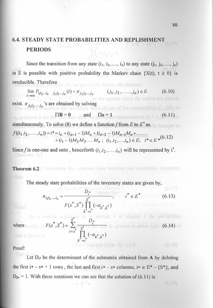
6.4. STEADY STATE PROBABILITIES AND REPLISHMENT

PERIODS

Since the transition from any state (i1, i2......, i„) to any state (j 15 j2,....., j„)

in E is possible with positive probability the Markov chain {X(t), t >- 0} is

irreducible. Therefore

Iiin Pili2 in 1112 in (1) -7:: "rjlj2 in (11,12........ in) E E (6.10)

exist . 2rj1J2••••• in's are obtained by solving

FIB=0 and IIe = 1 (6.11)

simultaneously . To solve (8) we define a function f from E to E* as

f((11,12 ).... .,In )) = 1 *=in +(in-1 - 1)Mn +(in-2 -1)Mn-1Mn.........(6.12)

+(il -1)M2M3..... M,1 ; (i1,i2,...,in) E E; 1* E E *

Sincef is one-one and onto , henceforth (i1 ,i2 .......i„) will be represented by i'

Theorem 6.2

The steady state probabilities of the inventory states are given by,

D. *1112......Jn - s*

F(s*,S*) f lk =i

i e E (6.13)

D.*where F(s • , S •) = Z, '* 1 (6.14)

* J1=S

fl- (-ak

Proof:

Let D;* be the determinant of the submatrix obtained from A by deleting

the first i* - s* + I rows , the last and first i* - s* columns, i* E E* - {S*}, and

Ds* = 1. With these notations we can see that the solution of (6.11) is

89

;Tili2.....in = iri* _

Di* 7rS*

S*-rR (-ak* k* )

k * =i

and Tr = 1r * =1

i* EE*-{S*} (6.15)

.1 S2 .....SnS -aS* S * I' (S* , S * )

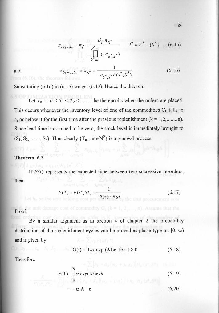
Substituting (6.16) in (6.15) we get (6.13). Hence the theorem.

(6.16)

Let To = 0 < TI < T2 < ........ be the epochs when the orders are placed.

This occurs whenever the inventory level of one of the commodities Ck falls to

sk or below it for the first time after the previous replenishment (k = 1,2.........n).

Since lead time is assumed to be zero , the stock level is immediately brought to

(S1, S2,........, Sn). Thus clearly { T,,, , mcN°} is a renewal process.

Theorem 6.3

If E(T) represents the expected time between two successive re-orders,

then

E(T) = F(s*,S*) =1

-aS*S* 7rS*(6.17)

Proof:

By a similar argument as in section 4 of chapter 2 the probability

distribution of the replenishment cycles can be proved as phase type on [0, oo)

and is given by

G(t) = 1-a exp (At)e for t > 0 (6.18)

Therefore

E(T) =Ta exp(A1)e di (6.19)0

= - a A-1 e (6.20)

(6.21)

= f-' (S *, S *) .

From (6.16), the theorem follows.

6.5 OPTIMIZATION PROBLEM

Let Mk* represent the random variable of the re-ordering quantity of

commodity Ck, then

E(Mk *)

S1 S2 S"

=E( I A k+ I I ..... I ;T'1'2i1=S1+1 i2=S2+1 in=Sn+1

(= E(T)[ A k+ ((Ok + qk ,u ) Hk (s*, S * )1

S1 S

where Hk Y 1i1=s1+1 i2=s2+

ik

ikwk + N A1EJk =°

Sn

I ik 7ci,i2.... inn=sn+1

/.

W

(6.22)

Let hk be the unit holding cost per unit time , ck the unit procurement cost

and dk the unit damage cost of commodity Ck (k = 1, 2 ......, n). Assume that the

fixed ordering cost for placing an order is K irrespective of the number of

different items ordered for replenishment . Therefore the cost function is

C(S1,S2...... Sn S1,S2

nK + I CkE(Mk *)

k=1

E(7-)n

+ [hk + dk (wk + p qk )]Hk (S*, S*) (6.23)k=1

^ik -Jk qlk

K= F,(s* S*) + I [Ck 4 + {(ck + dk)(wk + p qk) + hk }Hk (S* S*)]

k=1

91

Since shortages are not allowed and lead time is assumed to be zero it is

reasonable to expect that Sk = 0, (k = 1, 2....., n) for the optimum cost function.

Theorem 6.4

The cost function C(s1,s2,...s„ Si,S2,...S „) is minimum for si=s2=.... =s„= 0

Proof:

Suppose s 1 > 0. Let sl =I+ sn + si_1 Mn + sn_2 Mn_1 Mn +....+(sl -1) M2 ... Mn

Consider the matrix A = (d' 1'2 ln ) , (r , . . . . . . . . j , ) , , (IJ2 ...... J.,7 ) E ^'-o.... 3 1 32•••• Jn

where

1112.....1n J1J2 •••••Jn

r n

u+DA k+1kwk)k=1

10

Hr.',k=1 k/

Jk Ik -Jkk 9k

,7

^f D1k - Jk) > 1k=I

(lk-Jk )?0

otherwise

Let Dl* be the determinant of the submatrix obtained from A by deleting the

first i* - s1* + I rows, the last and first i* - s1* columns (i * S*), Ds* =1.

Then D ;* = D;* for i* E E * and D;* is positive for every i

11 12 Ik

+P PIP2........ Pk k = Jk k =1,2, .... n

9kk'1k -Jk ,HP' if ik -1k + 1,11 =./l (I= 1,2.....11; 1 # k)l=I

lk(6.24)

From (6.15) we get

92

F(s1 -1,s2,...,sn S1,S2....... Sn)=F(sl,S*)

S*Di

i *= Si fj-ak*,k*

k *=i

S* D s*-1

I Q* ,* + Ii *=s * l i *=s1

-ak*,k*)k*=i*

IDi*

71Di *

S* +1 -s II (-ak*,k*) i*-si II (-ak* k*

k *=i * k *=i

> F(s*, S*)

Also

S,H1 (s1 -1,s2, ... sn S1,S2. ... S,7)= I

1=s1

S, '2 Sn

= Sl + Y Z......

',=s,+1 i2=s2+1 in=sn+1

< Si +

S*

I

(6.25)

S2 Sn (11 - Si + s1 )Di*Y . . . . .. . . S*

i2=s2+1 in =S,,+1 F(s1,S*) (-ak* k*)

k *=i

('1 - s1)Di*

S*

f1 (-ak* k*)

k *=i *

(il - s1)Di*S*

1 ,S*) H(-aA.*,k*)

k *=i *

S*=,s* *F(.s*, S) (-ak* ,k*)

= H1(sl,s2,...s„ S1,S2.... Sn)

Thus, from (6.24) - (6.26) we have

C(s1 -1,s2...... Sn S1,S2...... S„) <C(sl,s2,...,s„ S1)S2...... ,S,,)

Therefore,

C(O,s2...... s„ S1,S2...... S,,) <C(s1,s2,...,Sn S1,S2....... S,,)-

by (6.25)

(6.26)

93

If sk > 0 for k > 1, then interchanging the position of s1 and sk we can

similarly prove that the cost function is minimum for Sk = 0 for each k. Hence

the theorem.

Let F(0, S*) = c(S*) and Hk(O, S*) = Wk(S*)

Then (6.24) will become

C(0,0,...,0 S1,S2...... Sn)= ^(S*) + [ck2k +{(ck +dk)(Wk +,ugk)+hk}n (S*)]k=1

(6.27)

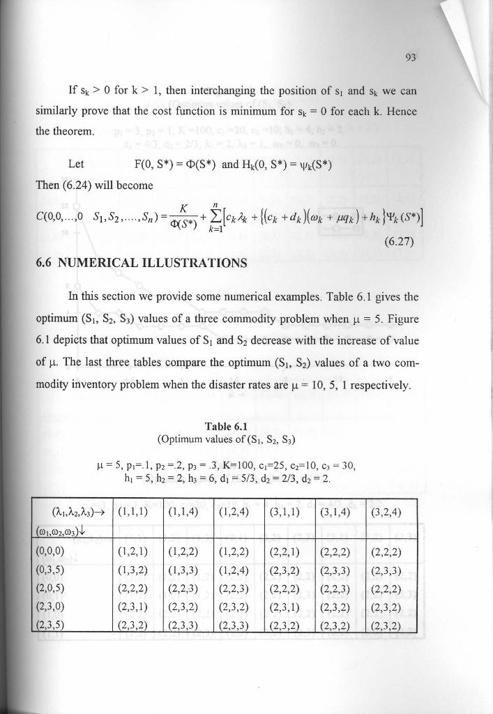
6.6 NUMERICAL ILLUSTRATIONS

In this section we provide some numerical examples. Table 6.1 gives the

optimum (S1, S2, S3) values of a three commodity problem when µ = 5. Figure

6.1 depicts that optimum values of S1 and S2 decrease with the increase of value

of µ. The last three tables compare the optimum (S1, S2) values of a two com-

modity inventory problem when the disaster rates are µ = 10, 5, 1 respectively.

Table 6.1(Optimum values of (S1, S2, S3)

µ = 5, p1=.1, p2 =.2, p3 = .3, K=100, c1=25, c2=10, c3 = 30,h1=5,h2=2,h3=6,d1=5/3,d2=2/3,d2=2.

(X1)X2,?13)->

((01,(02,(03 )y

(1,1,1) (1,1,4) (1,2,4) (3,1,1) (3,1,4) (3,2,4)

(0,0,0) (1,2,1) (1,2,2) (1,2,2) (2,2,1) (2,2,2) (2,2,2)

(0,3,5) (1,3,2) (1,3,3) (1,2,4) (2,3,2) (2,3,3) (2,3,3)

(2,0,5) (2,2,2) (2,2,3) (2,2,3) (2,2,2) (2,2,3) (2,2,2)

(2,3,0) (2,3,1) (2,3,2) (2,3,2) (2,3,1) (2,3,2) (2,3,2)

(2,3,5) (2,3,2) (2,3,3) (2,3,3) (2,3,2) (2,3,2) (2,3,2)

94

Figure 6.1(Optimum values of (S1, S2)

pl =.3, p2 =.1, K =100, c1 =20, c2 =10, h1 = 4, h2 = 2,

d1=4/3, d2=2/3, X1=2, X2= 1, w1=0, Q)2=0.

14 -r

0

0.50 I 2

Table 6.2(Optimum values of (S1, S2 when µ = 10)

--- s1

-(>- S2

2.5

p1=.3, p2 =.1, K=100, c1=20, c2=10, h1 = 4, h2 = 2, d1 = 4/3, d2 = 2/3

3

(?1,X2)- (1,1) (1,2) ( 1,3) (2,1) (2,2 ) (2,3) (3,1) (3,2) (3,3)

(0,0) (1,2) (1,2) ( 1,2) (2,2) (2,2) (2,2) (2,2 ) (2,2) (2,2)

(0,1) (1,2) (1,2) (1,2 ) (2,2) (2,2) (2,3) (2,2 ) (2,2) (2,3)

(1,0) (2,2) (2,2 ) (2,2) (2,2 ) (2,2) (2,2 ) (2,2) (2,2) (2,2)

( 1,1) (2,2) (2,2 ) (2,3) (2,2 ) (2,2) (2,3) (2,2) (2,2) (2,2)

95

Table 6.3(Optimum values of (Si, S2 when ^t = 5)

p1=.3, p2 =.1, K=100, c1=20, c2=10, h1 = 4, h2 = 2, d1 = 4/3, d2 = 2/3

(X1,X2)-* (1,1) (1,2) (1,3) (2,1) (2,2) (2,3) (3,1) (3,2) (3,3)

CO1,o2

(0,0) (2,2) (2,3) (2,3) (2,2) (2,2) (2,3) (2,2) (2,2) (2,3)

(0,1) (2,3) (2,3) (2,3) (2,2) (2,3) (2,3) (2,2) (2,3) (2,3)

(1,0) (2,2) (2,2) (2,3) (2,2) (2,2) (2,3) (3,2) (3,2) (3,3)

1 ) 1 (2,2) (2,3) (2,3 ) (2,2) (2,3) (2,3) (3,2) (3,3) (3,3)

Table 6.4(Optimum values of (Si, S2 when µ = 1)

p1=.3, p2 =.1, K=100, c1=20, c2=10, h1 = 4, h2 = 2, d1 = 4/3, d2 = 2/3

(X1,X2)-* (1,1) (1,2) (1,3) (2,1) (2,2) (2,3) (3,1) (3,2) (3,3)

C01,w2 `3

(0,0) (3,3) (3,5) (3,6) (4,3) (4,5) (4,6) (5,3) (5,4) (4,5)

(0,1) (3,4) (3,5) (2,6) (4,4) (3,5) (3,6) (4,4) (4,5) (4,6)

(1,0) (3,3) (3,4) (3,5) (4,3) (4,4) (4,5) (5,3) (5,4) (4,5)

(1,1) (3,4) (3,5) (3,6) (4,4) (4,5) (4,6) (4,4) (4,4) (4,5)

*****************