performance testing of coagulants to reduce stormwater ... · manual sampling ... figure 28. isco...
TRANSCRIPT

Technical Report Documentation Page 1. Report No.
FHWA/TX-14/0-6638-1 2. Government Accession No. 3. Recipient's Catalog No.
4. Title and Subtitle
PERFORMANCE TESTING OF COAGULANTS TO REDUCE STORMWATER RUNOFF TURBIDITY
5. Report Date
Published: May 2014 6. Performing Organization Code
7. Author(s)
Jett McFalls, Young-Jae Yi, Beverly Storey, Michael Barrett, Desmond Lawler, Brad Eck, David Rounce, Ted Cleveland, Holly Murphy, Desirae Dalton, Audra Morse, and George Herrmann
8. Performing Organization Report No.
Report 0-6638-1
9. Performing Organization Name and Address
Texas A&M Transportation Institute College Station, Texas 77843-3135
10. Work Unit No. (TRAIS)
11. Contract or Grant No.
Project 0-6638 12. Sponsoring Agency Name and Address
Texas Department of Transportation Research and Technology Implementation Office 125 E. 11th Street Austin, Texas 78701-2483
13. Type of Report and Period Covered
Technical Report: September 2010–August 2013 14. Sponsoring Agency Code
15. Supplementary Notes
Project performed in cooperation with the Texas Department of Transportation and the Federal Highway Administration. Project Title: Preparing for EPA Effluent Limitation Guidelines URL: http://tti.tamu.edu/documents/0-6638-1.pdf 16. Abstract
On December 1, 2009, the US Environmental Protection Agency (EPA) published a rule in the Federal Register establishing non-numeric and, for the first time, numeric effluent limitation guidelines (ELGs). The numeric ELGs included a turbidity limit of 280 nephelometric turbidity units (NTU) and sampling requirements for stormwater discharges from construction sites that disturb 20 or more acres of land at one time. At that time, the EPA required Texas to implement these new requirements when the Texas Commission on Environmental Quality (TCEQ) renewed their Texas Construction General Permit (CGP) in 2013. Due to litigation regarding the initial numeric ELG implementation, the EPA put numeric ELGs on hold in 2011 and on April 13, 2013, proposed to withdraw the numeric ELG as a requirement.
This project was initiated in 2010 to prepare the Texas Department of Transportation (TxDOT) for changes to the CGP regarding the monitoring and sampling of their construction site to meet the anticipated numeric ELG requirements. The scope of the project was modified due to EPA’s actions. However, in light of anticipated future numeric limits, the project’s monitoring and testing experiments proceeded to 1) determine “typical turbidity” representative of TxDOT’s construction site discharges, 2) collect performance data on innovative erosion and sediment control measures that might be expected to achieve the discharge standard, and 3) provide update to TxDOT’s Stormwater Managements Guidelines for Construction Activities. 17. Key Words
Effluent Limitation Guidelines, Stormwater, Turbidity, Flocculants, Coagulants, ELG, Erosion Control, Sediment Control
18. Distribution Statement
No restrictions. This document is available to the public through NTIS: National Technical Information Service Alexandria, Virginia http://www.ntis.gov
19. Security Classif.(of this report)
Unclassified 20. Security Classif.(of this page)
Unclassified 21. No. of Pages
86 22. Price
Form DOT F 1700.7 (8-72) Reproduction of completed page authorized

PERFORMANCE TESTING OF COAGULANTS TO REDUCE STORMWATER RUNOFF TURBIDITY
by Jett McFalls
Assistant Research Scientist Texas A&M Transportation Institute
Young-Jae Yi Post-Doctorate
Texas A&M Transportation Institute
Beverly Storey Associate Research Scientist
Texas A&M Transportation Institute
Michael Barrett Research Associate Professor University of Texas at Austin
Desmond Lawler Professor
University of Texas at Austin
Brad Eck Post-Doctorate
University of Texas at Austin
David Rounce Graduate Research Assistant University of Texas at Austin
Ted Cleveland Associate Professor
Texas Tech University
Holly Murphy Graduate Research Assistant
Texas Tech University
Desirae Dalton Research Assistant
Texas Tech University
Audra Morse Associate Academic Dean
Texas Tech University and
George Rudy Herrmann Graduate Research Assistant
Texas Tech University
Report 0-6638-1 Project 0-6638
Project Title: Preparing for EPA Effluent Limitation Guidelines
Performed in cooperation with the Texas Department of Transportation
and the Federal Highway Administration
Published: May 2014
TEXAS A&M TRANSPORTATION INSTITUTE
College Station, Texas 77843-3135


v
DISCLAIMER
This research was performed in cooperation with the Texas Department of Transportation
(TxDOT) and the Federal Highway Administration (FHWA). The contents of this report reflect
the views of the authors, who are responsible for the facts and the accuracy of the data presented
herein. The contents do not necessarily reflect the official view or policies of the FHWA or
TxDOT. This report does not constitute a standard, specification, or regulation.

vi
ACKNOWLEDGMENTS
This project was conducted in cooperation with TxDOT and FHWA. The authors thank
the TxDOT Project Monitoring Committee (PMC): Amy Foster, Jon Geiselbrecht, John Mason,
Kathleen Newton, and Tasha Vice. Jennifer Mascheck, TxDOT Bryan District, assisted the
researchers in locating projects for use monitoring sites.

vii
TABLE OF CONTENTS
Page List of Figures ............................................................................................................................... ix List of Tables ................................................................................................................................. x Introduction ................................................................................................................................... 1
C&G Rule Changes and Project Focus Impacts ......................................................................... 3 Literature Review ......................................................................................................................... 5
State Agency Construction General Permits ............................................................................... 5 Numeric Limits by Other States ................................................................................................. 6 Typical Runoff Turbidity from Construction Sites .................................................................... 6 Existing Construction Site Sampling Programs .......................................................................... 7
California Construction Site Sampling Requirements ............................................................ 7 Washington State Construction Site Sampling Requirements ................................................ 8 Oregon Construction Site Sampling ..................................................................................... 10
Controlled Testing of Coagulants .............................................................................................. 13 Erosion Control Performance Using Coagulants ...................................................................... 13
Facility and Equipment ......................................................................................................... 13 Materials and Methodology .................................................................................................. 16 Performance Test Procedure ................................................................................................. 19 Results ................................................................................................................................... 20
Sediment Control Performance Testing Using Coagulants ...................................................... 21 Facility and Equipment ......................................................................................................... 21 Materials and Methodology .................................................................................................. 23 Performance Test Procedure ................................................................................................. 24
Controlled Coagulant Tests ....................................................................................................... 25 Soil Sampling ........................................................................................................................ 25 Modified Synthetic Stormwater Runoff................................................................................ 26 Flocculants ............................................................................................................................ 27 Test Procedure ...................................................................................................................... 28
Construction Site Field Monitoring .......................................................................................... 31 Study Areas ............................................................................................................................... 31
Austin .................................................................................................................................... 31 Lubbock ................................................................................................................................ 32 College Station ...................................................................................................................... 34 Hearne ................................................................................................................................... 38 Bryan ..................................................................................................................................... 41
Sampling Methods .................................................................................................................... 43 Manual Sampling .................................................................................................................. 43 Automatic Sampling ............................................................................................................. 43
Results ....................................................................................................................................... 45 Grab Sampling in Austin ...................................................................................................... 45 Grab Sampling in Lubbock ................................................................................................... 46 Grab Sampling in College Station ........................................................................................ 46 Grab Sampling in Hearne ...................................................................................................... 49

viii
Grab Sampling in Bryan ....................................................................................................... 50 Automatic Sampling from Bryan .......................................................................................... 51
Conclusions and Findings .......................................................................................................... 55 Controlled Testing of Coagulants ............................................................................................. 55
Polyacrylamide for Erosion Control ..................................................................................... 55 Polyacrylamide for Sediment Control .................................................................................. 56 Coagulation and Dosing of Polyacrylamides ........................................................................ 57
References .................................................................................................................................... 63 Bibliography ................................................................................................................................ 65 Appendix A: State Numeric Standards for Construction Sites .............................................. 67 Appendix B: Typical Runoff Turbidity for Road Construction Projects from Previous Studies .......................................................................................................................................... 75

ix
LIST OF FIGURES
Page Figure 1. Hach SOLITAX® Model TS-line sc in situ Turbidity Sensor and Controller. ............. 15 Figure 2. Hach 2100N Turbidimeter. ............................................................................................ 16 Figure 3. Tested Erosion Control Blankets. .................................................................................. 18 Figure 4. Erosion Control Performance Tests Using Coagulants. ................................................ 20 Figure 5. Sediment Retention Device Testing Flume. .................................................................. 22 Figure 6. Wattle Used for Performance Testing. .......................................................................... 23 Figure 7. Decanter Used to Remove Large Particles from Soil Suspension. ............................... 27 Figure 8. Lubbock Project 1 – Marsha Sharp Freeway. ............................................................... 32 Figure 9. Lubbock Project 2 – West Loop 289. ............................................................................ 33 Figure 10. Lubbock Project 1 Discharge Locations. ..................................................................... 33 Figure 11. Lubbock Project 2 Discharge Locations. ..................................................................... 34 Figure 12. CS Project Watershed 1 Structure and Sampling Locations. ...................................... 35 Figure 13. CS Project Watershed 1. .............................................................................................. 35 Figure 14. Structure of CS Project Watershed 2. .......................................................................... 36 Figure 15. CS Project Watershed 2. .............................................................................................. 36 Figure 16. Structure of CS Project Watershed 3. .......................................................................... 37 Figure 17. CS Project Watershed 3 Vegetated Channel and Discharge to Creek. ........................ 37 Figure 18. CS Project Watershed 3 Relatively Flat Drainage Area with Loose Bare Soil. .......... 37 Figure 19. CS Project Watershed 3 Swale with Silt Fence on Bare Soil. ..................................... 38 Figure 20. Hearne Project Watershed 1 Swale with Rock Check Dam. ....................................... 39 Figure 21. Hearne Project Watershed 2 Concrete-Paved Channel. .............................................. 39 Figure 22. Hearne Project Watershed 3 Turbid Natural Creek. .................................................... 40 Figure 23. Hearne Project Watershed 4 Swale Covered by Rock Riprap. ................................... 41 Figure 24. Hearne Project Watershed 5 Swale Used as a Retention Basin. ................................. 41 Figure 25. Bryan Project Watershed 1 on Left and Watershed 2 on Right. ................................. 42 Figure 26. Bryan Project Watershed 3 Collection Points. ............................................................ 42 Figure 27. Bryan Project Watershed 4. ......................................................................................... 43 Figure 28. ISCO 6712 Sampler and ISCO 730 Bubbler Flow Module. ....................................... 44 Figure 29. Bryan Project Automatic Sampling Turbidity and Flow 1/9/2013. ............................ 52 Figure 30. Bryan Project Automatic Sampling Turbidity and Flow 4/2/2013. ............................ 52 Figure 31. Bryan Project Automatic Sampling Turbidity and Flow Depth 4/19/2013. ................ 53 Figure 32. Impact of Molecular Weight on Turbidity Reduction for Modified Synthetic
Stormwater Runoff for WLoop Soil. .................................................................................... 58 Figure 33. Effect of Charge Density on Flocculation for Modified Synthetic Stormwater Runoff
Using Wloop Soil. ................................................................................................................. 59 Figure 34. Most Effective Flocculants for Modified Synthetic Stormwater Runoff Wloop. ....... 60

x
LIST OF TABLES
Page Table 1. State CGP Expiration Dates. ............................................................................................. 5 Table 2. California’s Project Risk Level Matrix. ............................................................................ 7 Table 3. PAM Application Specifications. ................................................................................... 18 Table 4. Maximum Turbidity from Erosion Control Performance Tests. .................................... 21 Table 5. Average Dry Soil Loss from Erosion Control Performance Tests. ................................ 21 Table 6. Design Capacity and Ponding Volume of Wattles. ........................................................ 25 Table 7. Selected Properties of Soils Used in Laboratory Tests. .................................................. 26 Table 8. Molecular Weight and Charge Density of Flocculants. .................................................. 28 Table 9. Turbidity in Construction Site Runoff in Austin Area. .................................................. 45 Table 10. Turbidity in Construction Site Runoff in Lubbock Area. ............................................. 46 Table 11. CS Project Watersheds 1 and 2 Turbidities Readings of Samples. .............................. 47 Table 12. CS Project Watershed 3 Turbidities of Samples. .......................................................... 48 Table 13. Hearne Project Turbidities of Samples. ........................................................................ 49 Table 14. Bryan Project Turbidities of Samples. .......................................................................... 51 Table 15. Bryan Project Turbidity Change by Time Using Data from Automatic Sampling. ..... 51 Table 16. Maximum Turbidity from Controlled Erosion Control Tests. ...................................... 55 Table 17. Average Dry Soil Loss from Controlled Erosion Control Tests. .................................. 55 Table 18. Sediment Removal Efficiency of Untreated and PAM Treated Wattles. ..................... 57

1
INTRODUCTION
During the last two decades, there has been an increasing recognition by policy makers of
water quality impairment issues associated with sediment laden stormwater discharge from
construction sites. These issues led to several revisions and updates to the Clean Water Act of
1972. In December 2009 the US Environmental Protection Agency (EPA) issued new
nationwide discharge and monitoring standards for construction site stormwater runoff. These
new standards are the Effluent Limitations Guidelines and Standards for the Construction and
Development Point Source Category, known as the C&G Rule (74 FR 62995, 2009) (1). These
standards established non-numeric and, for the first time, numeric effluent limitation guidelines
(ELGs) and new source performance standards to control the discharge of pollutants from
construction sites. This new rule also specified that owners/operators of permitted construction
activities must:
Implement erosion and sediment controls.
Stabilize soils.
Manage dewatering activities.
Implement pollution prevention measures.
Prohibit certain discharges.
Utilize surface outlets for discharges from basins and impoundments (1).
The 2009 C&G Rule required that all sites disturbing 20 or more acres of land at one time
sample stormwater discharges and comply with a turbidity limitation of 280 nephelometric
turbidity units (NTU). At the time of the 2009 C&G Rule, all state environmental agencies were
required to incorporate these new regulations into their National Pollutant Discharge Elimination
System (NPDES) permits for construction activities when their construction general permits
(CGP) were re-issued. The Texas Commission on Environmental Quality (TCEQ) was set to
renew its Texas Pollutant Discharge Elimination System (TPDES) CGP in 2013 and anticipated
incorporating the numeric ELGs into its permit. The C&G Rule excluded projects covered under
an individual permit rather than being covered under the TPDES permit. These new regulations
would have been effective for any individual permit issued after February 1, 2010. In light of the

2
anticipated new requirements, the Texas Department of Transportation (TxDOT) was preparing
to meet the new regulatory requirements.
EPA’s decision to regulate turbidity through a numeric standard was based on the
agency’s conclusion that turbidity is an “indicator pollutant,” which will help identify other
pollutants coming from construction sites (1). The numeric ELGs set forth in EPA’s 2009 C&G
Rule consisted of the following:
Turbidity limit does not apply to stormwater discharges from storms that exceed the local
two-year, 24-hour storm.
On construction sites where the numeric limit applies, the rule requires contractors to
collect numerous stormwater runoff samples from all discharge points during every rain
event and measure the NTU level(s).
If the average NTU level of the samples taken over the course of a day exceeds the “daily
maximum limit” of 280 NTU on any given calendar day, then the site is in violation of
the federal limitation requirement.
EPA supposed that this standard could be met with passive treatment technologies, rather
than the advanced treatment systems, which EPA used as the technology basis for the draft limit
of 13 NTU.
The ELGs mandated by the EPA were considered a technology ‘floor’ that all permittees
would have been required to meet. As previously stated, each individual state regulatory agency
would have been required to include these minimum performance standards in their re-issued
construction general permit, and be allowed and encouraged to adopt more aggressive
requirements if they chose to do so. This left a number of requirements and decisions to the
authority of TCEQ.
As the EPA was preparing to make this new rule effective, they received petitions from
the National Association of Home Builders (NAHB), the Utility Water Act Group, and the
Wisconsin Builders Association for reconsideration of the rule. These petitions pointed out a
potential error in the calculation of the numeric limit. After examining the dataset underlying the
280 NTU limit, EPA concluded that it improperly interpreted the data and, as a result, the
original calculations used to establish the ELG were no longer adequate to support the 280 NTU
numeric effluent limit. The progress of the C&G Rule is as follows:
3
The EPA submitted a proposed rule to revise the turbidity limitation to the Office of
Management and Budget (OMB) in December 2010.
The EPA withdrew this proposal from OMB to seek additional performance data from
construction and development sites.
On January 4, 2011, the EPA acknowledged the error in calculating the 280 NTU effluent
limit and issued a direct final rule staying the limit until corrected. Because the numeric
limit for turbidity has been stayed, EPA and authorized states are no longer required to
incorporate the numeric turbidity limitation and monitoring requirements into their
permits.
On September 2, 2011, EPA filed a status report with the court indicating that it withdrew
the new numeric limit from OMB “to seek additional data on treatment performance from
construction and development sites.”
In December 2012, NAHB and EPA settled this matter. EPA has agreed to propose a rule
that vacates the numeric limit and modifies certain best management practice (BMP)
requirements. Furthermore, EPA will finalize the rule by February 2014, at which time
NAHB will formally drop its lawsuit (2).
On April 1, 2013, EPA decided to vacate the numeric standard and to add provisions to
improve the flexibility of the best management practices. EPA has added a definition for
“infeasible” that has a two part focus: 1) whether a control is “technologically possible”;
OR 2) whether it is “economically practicable and achievable in light of best industry
practices” (3).
C&G RULE CHANGES AND PROJECT FOCUS IMPACTS
This research project was initiated to prepare TxDOT for the anticipated changes to the
CGP regarding the monitoring and sampling of their construction sites to meet EPA’s numeric
ELG requirements. Another objective of this research project was to assist TCEQ with decisions
regarding the monitoring, sampling, and site management requirements of the EPA C&G Rule
by presenting the research results through TxDOT. Reducing sediment from stormwater runoff
is extremely beneficial to the quality of water sources. There was little doubt that the new

4
regulations mandated by EPA would have dramatically improved the nation’s waters if
developed and enforced correctly. Included in the original project objectives were the following:
Develop monitoring/sampling protocols.
Conduct statewide field testing to determine effectiveness of recommended practices and
sampling protocols.
Develop and conduct training/workshops for monitoring and sampling protocols.
TxDOT revised the project scope due to changes in the C&G Rule during the early stage
of the project. The PMC eliminated the above listed tasks from the project scope as they were
deemed premature at this time. However, there is still the generally accepted probability that the
EPA will eventually implement a numeric limit of some sort. In that, TxDOT decided to
continue with the data collection regarding construction site stormwater discharge and controlled
testing of various coagulant materials. Three research institutes, Texas A&M Transportation
Institute at College Station, the University of Texas at Austin, and Texas Tech University in
Lubbock, collaborated on the statewide data collection and experimentation regarding
differences in climate, soil types, slopes, and other factors that affect the performance of erosion
and sediment control measures. The project focused on the remaining tasks:
Review of literature and current state agency practices.
Controlled testing of coagulants.
Construction site field monitoring.
Revision of TxDOT’s Stormwater Managements Guidelines for Construction Activities.
One of the many issues regarding the sampling or monitoring requirements that may be
promulgated by EPA in the future is the potential for substantial costs, direct and indirect, to
permittees. These costs tend to be higher when associated to linear projects such as highways.
The scale and geometric configuration of highway projects typically crosses multiple watersheds
and, consequently, a large number of possible discharge locations. It may not be cost effective to
monitor all stormwater runoff from most highway construction sites. For example, a typical
5-mile long TxDOT construction site might be required to collect and sample more than 50
different locations. Future monitoring and sampling protocols will need to address these issues.

5
LITERATURE REVIEW
STATE AGENCY CONSTRUCTION GENERAL PERMITS
There are a number of states that have adopted turbidity construction runoff standards.
These states were identified to determine what these standards are and what practices have been
used by the respective departments of transportation (DOT) to meet these requirements. At the
time of the 2009 C&G Rule, authorized states were to incorporate the new rule requirements into
their reissued CGP, including any applicable numeric limits. For states needing to finalize their
CGP before the effective date of the corrected numeric limit, EPA advised them to issue their
permit without the numeric limit. Table 1 lists the CGP expiration dates for each state. EPA
encouraged these states to consider a shorter permit term in order to incorporate the corrected
limit sooner than five years. For states finalizing their CGP after the effective date of the
corrected numeric limit, but have to propose their permit prior to the effective date of the
corrected numeric limit, EPA encouraged them to pursue an approach similar to the one EPA
intends to follow so that they are assured of the ability to include the corrected limit in their final
permit.
Table 1. State CGP Expiration Dates.
State Expiration Year
South Dakota, Maine, Alabama, Michigan, Indiana, North Dakota, Pennsylvania, North Carolina
2009 or already expired
Connecticut, New York, Tennessee, Oregon, Washington
2010
Delaware, Wyoming, South Carolina, Vermont, Wisconsin, Arkansas, Kansas, Montana, New Hampshire, New Mexico, Idaho, Massachusetts
2011
Missouri, New Jersey, Colorado, Oklahoma, Nevada, Iowa, Hawaii, West Virginia, Nebraska
2012
Arizona, Ohio, Texas, Utah, Georgia, Illinois, Minnesota, Rhode Island, Maryland
2013
Florida, Kentucky, Virginia, California, Louisiana 2014

6
NUMERIC LIMITS BY OTHER STATES
While the EPA vacated their ruling on the numeric effluent limit for now, many states
already initiated a numeric limit, sampling programs, and analysis for sediment-related pollutants.
While the majority of states have not established a statewide standard, several states have their
programs well underway. These existing program values range from percent total suspended
solids (TSS) removal, NTU limits, pH range limits, and removal of pollutants compared to pre-
construction levels. Many more states have established post-construction standards. A table
listing each state and its current numeric standards for active construction sites is included as
Appendix A. The researchers did not include monitoring/sampling requirements for impaired
waters or specific water bodies such as cold water streams, etc.
TYPICAL RUNOFF TURBIDITY FROM CONSTRUCTION SITES
Previous studies showed a wide variance in runoff turbidity in roadway construction
projects (4, 5, 6). Based on the literature reviewed, the values ranged from 10 to 28000 NTU.
The California Department of Transportation (CALTRANS) monitored 15 highway construction
sites over a period between 1998 and 2000 (7). They selected 15 monitoring sites to represent a
wide range of CALTRANS construction site characteristics, considering construction type (e.g.,
roadway widening, new highway construction), construction activities (e.g., bridge, rail),
sampling location, and BMP in place. Their study reported turbidity readings from 15 to
16,000 NTU with an average turbidity of 702 NTU.
McLaughlin’s 2002 research (8) monitored three construction sites in North Carolina.
The selected sites were constructed on 1:2 fill slope of loam, 1:4 cut slope of loam, and 1:4 fill
slope of sandy loam, respectively. McLaughlin treated every site with two different surface
controls—polyacrylamide (PAM) only and PAM+mulch+seed. Runoff turbidities from those six
conditions varied from 11 to 5900 NTU through seven rainfall events. The sites treated with
PAM+mulch+seed produced less turbid water than the sites of PAM only. For example in 1:4 cut
slope site, the average turbidity was 2272 NTU in the PAM only site and 182 NTU in the
PAM+mulch+seed site (refer to Appendix B for more detail).
McLaughlin and Jennings focused on the performance of erosion and sediment control
measures on construction sites (9). For erosion control measures, they installed excelsior erosion

7
control blanket, hydromulch, and straw on active construction sites and monitored runoff
turbidities for four to six rainfall events by site. The maximum turbidity in the tests reached over
24,000 NTU. Sites treated with sediment control measures, including 14 types of sediment traps
and basins, yielded 8 to 30,000 NTU of runoff. They also monitored final outlets discharging to
nearby streams and found 116 to 2950 NTU of average daily turbidity (see Appendix B).
EXISTING CONSTRUCTION SITE SAMPLING PROGRAMS
California, Washington State and Oregon have established effluent limits and sampling
procedures for their construction sites. Following is a brief description of each program.
California Construction Site Sampling Requirements
The California Environmental Protection Agency State Water Resources Control Board’s
Construction General Permit includes a risk-based permitting approach by requiring project site
risk assessment (10). This risk assessment is based on two criteria:
Project sediment risk is assessed based on site characteristics (slope steepness, soil type,
etc.) and project scheduling (wet/dry season, construction work window, etc.). The
Revised Universal Soil Loss Equation (RUSLE) is used to determine the sediment risk.
Receiving water risk is assessed based on whether or not the receiving water is listed on
303(d) list, been released a total maximum daily load (TMDL) for sediment, or chosen as
Cold/Spawn/Migratory.
The results of the two risk assessments classify the project site into risk levels 1 – 3 as
shown in Table 2. Sampling and monitoring requirements are varied by risk levels.
Table 2. California’s Project Risk Level Matrix. Sediment Risk Low Medium High Receiving Low Level 1 Level 2 Water Risk High Level 2 Level 3

8
Visual Monitoring
All projects, regardless of risk level, require quarterly visual inspections at three levels—
non-storm, storm-related, and post-storm. Non-storm inspections are conducted to check
stormwater control devices. Storm-related inspections must be done by visually observing
stormwater discharges at all discharge points within two business days following a rain event.
Post-storm inspections must be conducted to recognize the effectiveness of stormwater control
devices.
Effluent Monitoring
Sites selected as risk levels 2 or 3 require sampling and effluent analysis. Sampling must
be conducted after a rainfall event over 0.5 inches at the time of discharge. The sampling
requirements are as follows:
Risk level 1 requires visual monitoring.
Risk level 2 requires effluent sampling.
o Turbidity: 250 NTU numeric limit
o pH: 6.5 – 8.5
Risk level 3 requires effluent monitoring and bio-assessment (limited cases).
o Turbidity: 500 NTU numeric limit
o pH: 6.0 – 9.0
Risk level 2 and 3 monitoring
o A minimum of three samples per day must be collected from discharge sites
following a qualifying rain event (half inch or more at the time of discharge) (10).
Washington State Construction Site Sampling Requirements
The stormwater monitoring program of the Washington State Department of Ecology
suggests the basics for site inspections and stormwater sampling. The program determines
whether or not BMPs are working correctly and explains the proper protocol to measure the
turbidity of discharge from construction projects.

9
Sampling Methods
The program suggests two methods to measure turbidity, 1) transparency tube method
and 2) turbidimeter method. Water sampling is not required in construction projects that disturb
less than one acre. Sites of one to five acres may use either method. Turbidimeter method is
required for projects with disturbed areas greater than five acres. Construction projects that use
1000 cubic yards of concrete must sample for pH. Also, the Washington Department of Ecology
may demand additional monitoring for projects that release into a 303(d) listed water body or
designate a TMDL.
Turbidity and transparency samples are collected at all stormwater discharging points
including ditches, pipes, drains, and detention/retention pond discharges. Samples for pH
monitoring must be collected before discharge occurs. The program requires weekly sampling
and within 24 hours of a rainfall when stormwater discharge occurs. This protocol intends to
make all samples representative of the total discharge from the project site.
The program suggests three sampling methods—single grab sample, time-proportionate
sample, and flow-proportionate sample. Any of these methods can be used as long as it achieves
a representative sample of the stormwater runoff. Some principles for sampling are listed in the
program such as:
Use clean gloves and collection bottles.
Avoid disturbing flow bottom.
Avoid touching the opening of the bottle.
Hold bottle to make flows come from upstream directly into the bottle.
Stand downstream.
Keep bottle lids off the ground.
Label each sample instantly after collection.
Capture a sample with a scoop in order not to disturb bottom settlements (11).
Visual Monitoring
The Washington State monitoring program requires visual inspection by experts for
possible signs of erosion, suspended sediment, turbidity, discoloration, and oil sheen in
stormwater runoff.

10
Oregon Construction Site Sampling
Oregon uses a 160 NTU benchmark for stormwater runoff turbidity on construction sites.
Oregon Department of Environmental Quality’s General Permit National Pollutant Discharge
Elimination System Stormwater Discharge Permit 1200-C (12) includes analysis of the runoff
turbidity from construction sites to determine if BMPs perform effectively to meet the turbidity
benchmark. The permit describes minimum measurement requirements for the monitoring,
including when and where measurements should be monitored, how samples should be collected,
and what needs to be inspected.
The Oregon permit designates three major areas of interest for turbidity measurements on
construction sites and requires corrective action if the turbidity is too high at these areas. These
locations include:
Locations where the discharge eventually leads to surface waters either directly or
through a conveyance system.
Fifty feet downstream from discharge points that lead to surface waters.
Any place where the discharge into surface waters is greater than half of the width of the
collecting water body (12).
Visual Inspection
Oregon requires visual inspection and turbidity measurement. The visual inspection of
erosion and sediment controls is conducted differently depending on the site condition as follows:
In active construction sites, visual inspection should be conducted every day when
stormwater runoff exists.
Visual inspection should be done once before the construction is completed or the site
becomes inaccessible.
When the site is inactive for longer than seven days, inspection should be done every
other week.
When the site becomes inaccessible due to severe weather, inspection is recommended
once a day if possible.

11
Visual inspections should describe the color and clarity (turbidity). The color should be
compared to nearby surface waters, and any sheen or floating material in the runoff should be
visually inspected. If the site is inaccessible, inspection should be recorded downstream of the
discharge point.
Sampling and Turbidity Measurement
Turbidity should be measured at all discharge points where stormwater flows directly or
indirectly to surface water. At least one sample representative of the stormwater runoff should be
collected at every monitoring point. A field turbidimeter should be used to measure turbidity.
Sampling frequency and condition is conducted once a week when stormwater runoff is
present. Sampling instruction states that samples should be taken before the runoff reaches
another body of water or substance in order to ensure the representativeness of samples. The
permit suggests the grab sampling method and instructs that each sample collected over a period
of time not to exceed 15 minutes.


13
CONTROLLED TESTING OF COAGULANTS
One sediment reduction treatment demonstrating much promise is the use of settling
agents known as coagulants, such as polyacrylamide (PAM), chitosan, alum, and gypsum. When
added to the stormwater flow these products reduce the charges on the colloidal clay suspensions
allowing them to flocculate or clump/mass together and, therefore, settle out of suspension. The
terms coagulation and flocculation are often used interchangeably; however, coagulants are the
products used to destabilize the charged colloidal particles, and flocculation is the mixing of
these products to promote the agglomeration of the stabilized particles. Research indicates that
these agents can substantially reduce the turbidity of discharged stormwater.
Performance evaluations of coagulants were conducted at the Texas A&M Transportation
Institute’s (TTI) Hydraulics, Sedimentation, and Erosion Control Lab (HSECL), using an indoor
rainfall simulator (erosion control tests) and a sediment retention device testing flume (sediment
control tests). The Center for Transportation Research in Water Resources (CTR) at The
University of Texas in Austin conducted laboratory tests using different soils and coagulants.
Erosion and sediment control tests evaluated the field application performance of flocculants
(PAM) used in conjunction with standard erosion and sediment control products. The objective
of CTR testing was to develop an understanding of how soil characteristics and polymer
properties affect the amount of turbidity reduction that can be achieved through flocculation.
EROSION CONTROL PERFORMANCE USING COAGULANTS
Facility and Equipment
The indoor rainfall simulator at the HSECL has two soil beds that can be adjusted to any
desired slope up to 1:2 (or 50 percent). The rainfall simulator provides a water drop size
distribution and impact velocity typical of severe storms that occur in Texas and the Gulf Coast
regions of the country. The rainfall simulator is designed to subject test beds of selected soil fill
to very destructive rainfall characteristics and high rainfall rates. Simulated rainfall is dropped
from a height of 14 ft above the test bed which provides 85–90 percent terminal velocity with an
average drop size of approximately 4.4 mm.

14
Researchers conducted erosion control performance evaluation tests using PAMs and
rolled erosion control blankets in the HSECL indoor rainfall simulator. The test parameters were
as follows:
Test bed: 30 ft × 6 ft on 1:3 slope.
Rainfall duration and rate: 30 minutes at 3.5 inches/hr.
Soil type: clay (tests on sand plots were excluded because PAM is known as less
effective on sandy soils).
Soil moisture: less than 70 percent (determined by a Kelway model 36 moisture meter).
Researchers measured total sediment loss and turbidity from each test. Midway through
the testing process researchers changed the turbidity measurement method from an automated
monitoring system to a manual grab sampling. The initial automated system was designed to
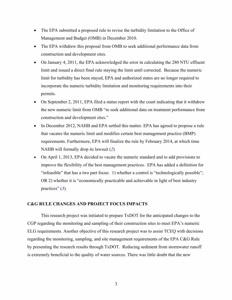
record turbidity at one minute intervals using the Hach SOLITAX® model TS-line sc (see Figure
1) in situ turbidity sensor. After recognizing that the flow rates from test runoffs were too low to
acquire reliable readings from the sensor, researchers grabbed samples at five minute intervals
and measured turbidity using the Hach 2100N turbidimeter shown in Figure 2. The total
sediment loss was measured using a consistent protocol through the entire test procedure.
The Hach SOLITAX® model TS-line sc sensor was connected to a Hach model sc100
controller system. Datacom software available on the Hach website enabled the retrieval of the
turbidity data from the controller system to a field laptop. Specifications of the turbidity sensor
are as follows:
Measuring range: 0.001 to 4000 NTU.
Accuracy: less than 1 percent of reading or ±0.001 NTU, whichever is greater.
Signal average time: user selectable ranging from 1 to 300 sec.
15
The specifications of the Hach 2100N turbidimeter used for the grab-sample tests are as
follows:
Measuring Range: 0 to 4000 NTU with ratio on.
Accuracy: ± 2 percent of reading plus 0.01 NTU from 0 to 1000 NTU.
±5 percent of reading from 1000 to 4000 NTU.
Lamp Type: Tungsten.
Operating temperature range: 0 to 40°C.
Regulatory: EPA method 180.1.
Repeatability: ± 1 percent of reading or ± 0.01 NTU, whichever is greater.
Resolution: 0.001 on lowest range.
Response Time: 6.8 sec with signal averaging off; 14 sec with signal averaging on.
Sample cell compatibility: 25 mm round; 12, 13, 16, and 19 mm round with optional
adapter kit.
Figure 1. Hach SOLITAX® Model TS-line sc in situ Turbidity Sensor and Controller.

16
Figure 2. Hach 2100N Turbidimeter.
Materials and Methodology
TTI researchers evaluated the performance of PAMs for erosion control using the
HSECL’s indoor rainfall simulator where they compared PAM-treated conditions with non-
treated conditions. Erosion control testing used two PAM products and three types of rolled
erosion control blankets (ECB) (i.e., jute, excelsior, and straw) as shown in Figure 3. A total of
eight treatments were tested as follows:
Bare ground vs. PAM on bare ground.
Jute ECB vs. PAM on jute ECB.
Excelsior ECB vs. PAM on excelsior ECB.
Straw mulch ECB vs. PAM on straw mulch ECB.
PAM products are generally recommended to use with ECBs because a sole application
of PAM results in limited performance. This study tested the performance of two PAM products,
PAM1 and PAM2, in conjunction with ECBs consisting of jute, excelsior, and straw.
PAM1 is an anionic polyacrylamide copolymer. Technical specifications are as follows:
Viscosity: 2410 cps.
Insoluble: 4–5 maximum.
Residual acrylamide (ppm): < 500 (0.05 percent).
Dry content percentage: 90.0 minimum.
Anionic charge percent: 30 ± 1.0.

17
Approximate molecular weight: 12–15 mg/mol.
Maximum concentration: 5g/l.
Recommended application rate: 9 lb/acre (1:3 slope).
PAM2 is another anionic linear copolymer of acrylamide. The specification for this
product is as follows; however, some proprietary information (including anionic charge percent
and molecular weight) was not made available by the manufacturer:
Bulk density: 40–50 lb/ft3.
Percent moisture: 15 percent maximum.
pH 0.5 percent Solution: 6–8.
Recommended application rate: 20–35 lb/acre (1:3 slope, clay soil).
The jute ECB used was 100 percent polypropylene. Its technical information is as follows:
Polypropylene 1/8 inch square mesh.
2.5 oz/yd2.
Multifilament and tape yarn weave.
Photo degradable.
The excelsior ECB consists of a 100 percent certified weed free straw matrix stitched to a
single net. Its technical information is as follows:
Stitch spacing: 2 inches on center.
Unit weight: 8.0 oz/yd2.
Thickness: 0.28 inch.
Tensile strength, MD: 4.8 lb/inch.
The straw ECB used is a 100 percent agricultural straw blanket with straw fibers stitched
between two photodegradable nets using photodegradable thread. Its technical specifications are
as follows:
Mass/unit area: 8.3 oz/yd2.
Tensile strength: 75 lb/ft.

18
Thickness: 0.25 inch.
Light penetration: 16 percent.
Water absorption: 461 percent.
Elongation, MD: 21.6 percent.
Permissible shear stress: 1.75 lb/ft.
Permissible rate of flow: 6 ft/sec.
(a) Jute ECB (b) Excelsior ECB (c) Straw ECB
Figure 3. Tested Erosion Control Blankets.
Table 3 presents the PAMs and erosion control blanket application specifications. PAM1
was applied with excelsior blanket and straw blanket, and on bare soil. These treatments were
applied in liquid form using a hydroseeder because the application rates were not great enough
for broadcast treatment. PAM2 was applied with the jute ECB. Since PAM2 caused clogging of
a hand-held hydroseeder, researchers broadcasted the PAM2 powder on the jute ECB netting.
Table 3. PAM Application Specifications. Treatment PAM Application Rate PAM Application Method
PAM1 9 lb/ac Hydroseeder PAM1 + Excelsior ECB 9 lb/ac Hydroseeder
PAM1 + Straw ECB 9 lb/ac Hydroseeder PAM2 + Jute ECB 25 lb/ac Broadcast

19
Performance Test Procedure
The TTI research team conducted the following procedures for the preparation of the soil
filled test beds, installation of materials, and rainfall simulation process:
Till soil-filled test bed and bring to a saturation point of less than 70 percent.
Level the test bed using heavy equipment and a pipe drag. When leveled, compact the
test bed soil fill cross-slope using a 150-lb hand roller. When last measured with a
nuclear density meter in 2010, clay compaction was 89.3 percent of optimal density.
Install test materials using exact manufacturer’s instructions for staple pattern and/or rate
per acre for spray on products. For this study, researchers applied the PAM products
using a broadcast or hydroseed method.
Test ECB materials the same day of installation.
Roll the prepared test bed into the rainfall simulator and lift into position (1:3 slope)
using the overhead drum hoist.
Conduct simulated rainfall for 30 minutes per test bed at a rainfall rate of 3.5 inches per
hour (198 gallons water added for each test).
Collect all water and sediment using containers or collection sacks.
Allow collected water and sediment to settle overnight to enable the separation of the
water and sediment.
Decant and weight the separated water for each container.
Collect three random 1 pint grab samples from the sediment containers after weighing
and take these samples to the HSECL index testing laboratory to completely dry to
determine the percent moisture content.
Subtract the moisture percentage of the grab samples from the total sediment loss weight.
For example a dried 100-lb sample of sediment had 25 percent water. Subtract the
25 percent from the total batch weight. Record the 75-lb dry weight as actual soil loss.
Repeat the process after a 24-hour waiting period from the previous rainfall test. Repeat
the exact same rainfall test and subsequent soil weighing and moisture determination
process two more times for two consecutive days on each of the test beds. The testing
process consists of three simulated rainfall events on three consecutive days.
20
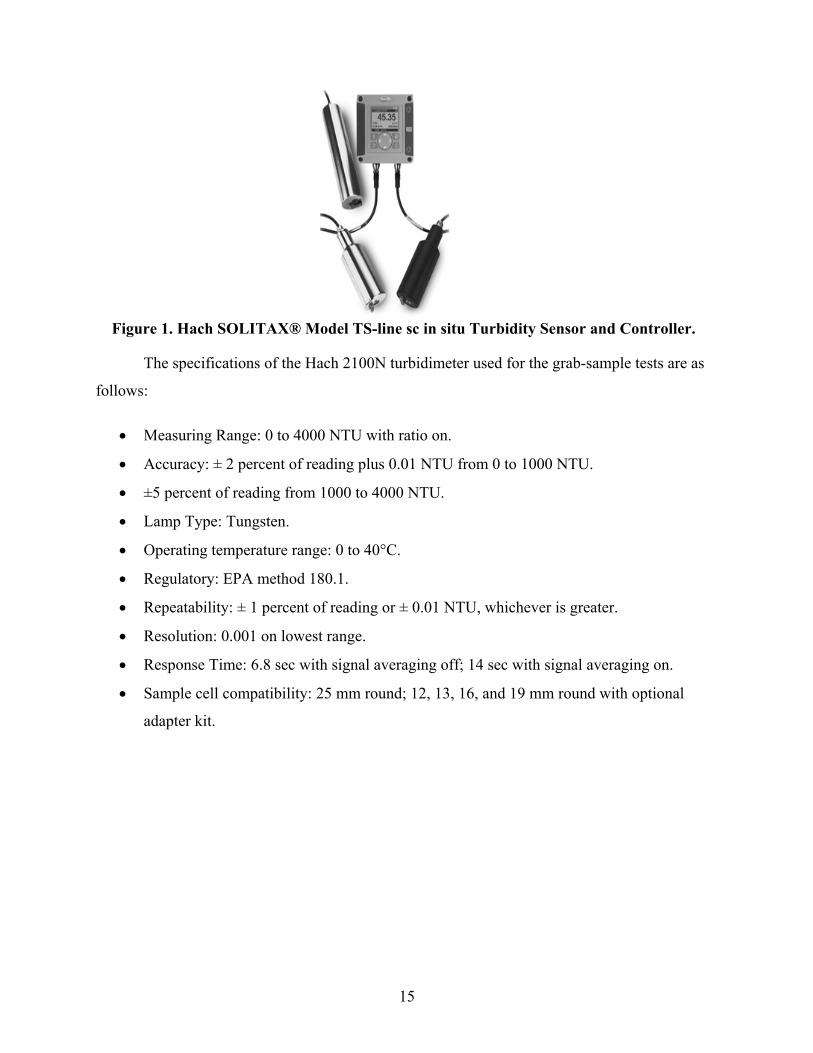
Combine the dry sediment loss from all three tests to determine total soil loss.
Average the soil loss from all three rounds to determine a final total sediment loss.
Figure 4 shows an example of how the erosion control testing uses the in situ turbidity
sensor on a weir box to collect turbidity and flow rate data automatically.
Figure 4. Erosion Control Performance Tests Using Coagulants.
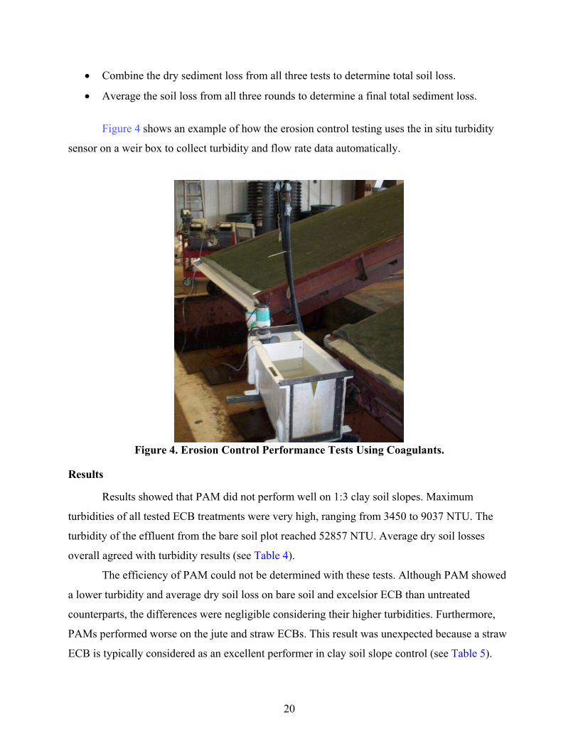
Results
Results showed that PAM did not perform well on 1:3 clay soil slopes. Maximum
turbidities of all tested ECB treatments were very high, ranging from 3450 to 9037 NTU. The
turbidity of the effluent from the bare soil plot reached 52857 NTU. Average dry soil losses
overall agreed with turbidity results (see Table 4).
The efficiency of PAM could not be determined with these tests. Although PAM showed
a lower turbidity and average dry soil loss on bare soil and excelsior ECB than untreated
counterparts, the differences were negligible considering their higher turbidities. Furthermore,
PAMs performed worse on the jute and straw ECBs. This result was unexpected because a straw
ECB is typically considered as an excellent performer in clay soil slope control (see Table 5).

21
Table 4. Maximum Turbidity from Erosion Control Performance Tests.
Surface Condition No PAM Treated PAM Treated Difference
Bare soil 52857 NTU 51987 NTU −870 Jute ECB over 4040* NTU over 4040* NTU NA
Excelsior ECB 3603 NTU 3450 NTU −153 Straw ECB 4180 NTU 9037 NTU +4857
* over the capacity of the in situ turbidity sensor Table 5. Average Dry Soil Loss from Erosion Control Performance Tests.
Surface Condition No PAM Treated PAM Treated Difference
Bare soil 175.50 lb 163.10 lb −12.40 Jute ECB 17.25 lb 19.05 lb +1.80
Excelsior ECB 6.97 lb 5.43 lb −1.54 Straw ECB 0.40 lb 10.17 lb +9.77
Several potential reasons came from the observation of tests. First, broadcast application
might limit the efficacy of PAMs. The PAM2 hand-broadcasted on the jute ECB did not develop
obvious flocculation during the tests; consequently, the dry soil loss of its effluent was nearly
equivalent with the untreated jute ECB. However, the PAM1 applied with the hydroseeder on
straw ECB created very viscous flocculation from the plot surface to the outlet. It was expected
that those flocculated sediments were stuck into the straw ECB, but in reality, the sediment clogs
appeared too heavy to be held on the blanket surface, particularly with the heavy design storm
(3.5 inches/hr). Also, the PAM1 appeared to facilitate more flocculation by softening surface soil.
SEDIMENT CONTROL PERFORMANCE TESTING USING COAGULANTS
The performance of PAM in sediment controls or sediment retention devices (SRD) was
evaluated by comparing a PAM-treated wattle with non-treated wattle. Tests were conducted at
the HSECL using the SRD flume.
Facility and Equipment
The SRD flume has a 12-ft upper flume and a 2-ft lower flume as shown in Figure 5. The
soil-filled area is 4-ft wide soil-filled and is used to install the material according to
manufacturer's specifications. The reservoir is a 1600-gal polypropylene cylindrical tank with a
conical hopper bottom with a 6-inch butterfly valve. A 3-phase electric motor and double mixing
paddles ensure proper mixing of the sediment-laden test water. The reservoir continually mixes

22
slurry of well-graded artificial sediment. Turbidity meters monitor influent and effluent
concentrations. Flow meters monitor influent and effluent flow rates. The SRD flume is made up
of three distinct zones: the retention zone, the installation zone, and the collection zone. The
overall length of the channel is 18 ft.
The retention zone is a longitudinal section of a cylinder 25 ft in diameter 12 ft long, and
15 ft wide with a maximum depth of 2.5 ft. The channel maintains a constant 3 percent
slope. The concrete flume has a waterproofing grout surface.
The installation zone is a 4-ft opening between the retention zone and collection zone
with metal sliding gates on either side. The installation zone can be filled with any type
of test soil. The proposed soil for testing SRD’s is high plasticity index (PI) clay. The
surface of the clay in the installation zone was shaped to match the profile of the channel.
The designed shape of the collection zone matches the retention zone except it is only 2 ft
long. The collection zone provides an area to channel the flow toward the collection and
monitoring system.
Figure 5. Sediment Retention Device Testing Flume.
Turbidity is measured with the Hach SOLITAX® model TS-line sc in situ turbidity
sensor connected to the Hach SC100 controller.
Two ISCO® model 4230 bubbler flow meters monitored the flow at inlet and outlet of
the SRD flume. This bubbler flow meter uses an internal air compressor to force a metered
amount of air through a bubble line submerged in the flow channel. The flow level is accurately

23
determined by measuring the pressure needed to force air bubbles out of the line. Its brief
specifications are as follows:
Range: 0.1 to 10 ft.
Level measurement accuracy: ±0.005 ft from 0.1 to 5.0 ft.
Materials and Methodology
The tested wattle was a composite of wood fibers and crimped man-made fibers encased
in a heavy duty, knitted cylindrical tube as shown in Figure 6. The design capacity and ponding
volume of tested wattles are as follows:
Height: 4.25 inches.
Design capacity: 65 gal.
Ponding volume: 59–63 gal (non-treated) and 66 gal (treated).
Figure 6. Wattle Used for Performance Testing.
The tests controlled the mass loading of inflow and measured the difference in the mass
loading of outflow. The controlled properties of the inflow are as follows:
Sediment: Silica (Sil-Co-Sil® 49) 12.5 lb and ball clay 12.5 lb.
Water volume: 70 gal.
Slurry concentration: 2000 mg/L.

24
The mass loading of outflow was estimated using flow rate and turbidity monitored at the
one minute resolution. The following data was recorded and calculated for each product
evaluation:
Flow-through rate (cfs).
Maximum flow rate at gallons per minute (gpm).
Ponding volume (gal).
Turbidity (NTU) at inlet and outlet.
Suspended sediment concentration (SSC) (mg/L) at inlet and outlet.
Mass loading (lb).
Removal efficiency as percentage.
Performance Test Procedure
The TTI research team conducted the following procedures for the preparation of the
SRD flume, installation of materials, and flume flow process. Table 6 shows the results of the
SRD flume tests using the treated and untreated wattles.
Researchers cleaned the SRD flume and resurfaced the soil in the installation zone to
match the flume profile.
The SRD was installed in the installation zone according to manufacturer’s instructions.
The turbidity probes and bubbler tubes were connected to the appropriate locations at
inlet and outlet.
A mix of 12.5 lb of SIL-CO-SIL®49 and 12.5 lb of ball clay was placed in 1500 gal of
water to create sediment-laden water having a SSC of 2000 mg/L. The sediment laden
water was continually stirred in the mixing tank throughout the test.
The water slurry was released into the flume, at a flow rate defined by the SRD flow
category, by controlling the butterfly valve on the mixing tank. The entire 1500 gal of
sediment-laden water was emptied into the flume.
The test monitoring continued until there was no water retained behind the SRD.
Three repetitions of this test were conducted on SRD before removing it from the
installation zone.

25
Table 6. Design Capacity and Ponding Volume of Wattles. Sediment Retention
Device Test
Round Height
Inches (cm)Design Capacity
Gal (L) Ponding Volume
Gal (L)
Wattle – untreated 1 4.25 (10.8) 65 (246) 59 (223) 2 4.25 (10.8) 65 (246) 60 (227) 3 4.25 (10.8) 65 (246) 63 (238)
Wattle – treated 1 4.25 (10.8) 65 (246) 66 (250) 2 4.25 (10.8) 65 (246) 66 (250) 3 4.25 (10.8) 65 (246) 66 (250)
CONTROLLED COAGULANT TESTS
Recent field use and research indicates that soil characteristics have an important bearing
on the effectiveness of specific coagulants and that no single type is effective in reducing
sediment from all sediment sources. For coagulants to be effective on TxDOT construction sites
laboratory testing determined effectiveness and dosing of various coagulants for various soil
types. Researchers conducted tests on a variety of soil types representative of those encountered
statewide in highway construction projects. The coagulants evaluated included a variety of
polymers, chitosan, and other chemicals.
Soil Sampling
Seven soil samples were collected at highway construction sites from across the state of
Texas through collaboration with The University of Texas at Austin, Texas A&M Transportation
Institute, and Texas Tech University. Grab samples of soils were collected from spoil piles. The
spoil piles are representative of the fill material typically used in the construction of highways
and are most vulnerable to being transported in the stormwater runoff from construction sites.
Midwest Laboratories, Inc. (Omaha, Nebraska) analyzed the properties of these seven soil
samples as shown in Table 7. As is standard practice in soil analysis, the designation of sand, silt,
and clay is based on the weight percent in various particle size ranges, with sand being all
material > 62.5 μm, clay being all material < 2 μm, and silt being everything in between.

26
Table 7. Selected Properties of Soils Used in Laboratory Tests.
Sample pH Ca
(mg/ kg)
Mg (mg / kg)
CECa
(meq / 100g)
OrganicMatter
(%)
Sand (%)
Silt (%)
Clay (%)
183ANBC 8.2 4618 149 24.9 1.1 28 36 36
College Station 9.28 3956 231 22.2 1.6 38 40 22
W Loop 8.3 3222 434 20.7 0.7 52 28 20
127 Lub 7.8 2066 509 16.6 0.7 58 22 20
Hearne I 4.8 1195 371 17.8 1.5 18 30 52
Hearne II 7.8 569 64 3.5 0.2 86 6 8
E Texas 5.0 621 134 7.4 0.5 60 12 28 a Cation exchange capacity
Modified Synthetic Stormwater Runoff
A modified synthetic stormwater runoff was created for each soil sample such that it had
a turbidity of 1500 NTU (±300 NTU). The turbidimeter used for synthetic runoff and jar tests
was a Hach Ratio/XR Turbidimeter (Hach Company, Loveland, CO) and has an upper limit of
2,000 NTU. Therefore, 1500 NTU was selected as a standardized value, so that a comparison
could be made between modified synthetic runoff of similar initial turbidities. By creating a set
of samples with similar turbidity but from different soil types, the laboratory evaluation could
focus on the effects of the soil characteristics directly and exclude the effects of overall particle
(mass) concentration.
The modified synthetic stormwater runoff was prepared through an iterative approach.
A six liter soil suspension of 15 g/L was prepared in the decanter shown in Figure 7.
This soil suspension was then rapid mixed mechanically for five minutes.
The suspension was then allowed to settle for 2 minutes and 37 seconds. This time
allows large particles that would typically settle out quickly in runoff to settle out of the
modified synthetic stormwater runoff being created. Accounting for Stokes’ Law and the
height of the ports on the decanter, 2 minutes and 37 seconds should allow all particles
25 μm and larger to settle out of the suspension.

27
A sample of the soil suspension was then taken and measured for turbidity. If the soil
suspension’s turbidity was less than 1,200 NTU, then a known amount of soil was added
to the suspension and the process was iterated.
This process was repeated until the soil suspension’s turbidity fell within the specified
range of 1,200 to 1,800 NTU.
Once this target turbidity was obtained, the process was iterated one more time without
adding any soil and after 2 minutes and 37 seconds, the soil suspension was decanted into
a large storage container.
This process was repeated at least three times such that over nine liters of modified
synthetic stormwater, runoff was created for each soil for use in laboratory tests.
Figure 7. Decanter Used to Remove Large Particles from Soil Suspension.
Flocculants
The nine flocculant products used in this study covered a range of molecular weights and
charge densities (see Table 8). The molecular weight of the polyacrylamides ranged from 0.2 to
14 mg/mol, and the charge densities ranged from neutral to 50 percent anionic molar charge.
Cationic PAM products were not included in this study due to their toxicity to aquatic life.
Researchers included a cationic polymer, chitosan, in this study due to its effectiveness as a
positively charged polymer. Stock solutions of PAM (0.1 g/L and 10 g/L) were prepared with DI
water and stirred for 24 hours at room temperature.

28
Table 8. Molecular Weight and Charge Density of Flocculants. PAM Type Molecular Weight (mg/mol) Charge Density (%) SF N300 15 Neutral
LMW SF N300 6 Neutral A 110 10-12 16 A 130 10-12 33 A 150 10-12 50
A 110 HMW 10-14 16 Cyanamer P-21 0.2 10
Chitosan NA Positive APS #705 NA NA
Test Procedure
The research team used a Dekaport Cone Sample Splitter (Rickly Hydrological Company,
OH) to create homogeneous samples of the modified synthetic runoff for each individual jar test.
The large collection container was mixed well, and the contents were poured into the top of the
splitter. The splitter divided the modified synthetic runoff into 10 Erlenmeyer flasks. From these
flasks, 200 mL of modified synthetic runoff were measured and poured into the jars for testing.
The jars were specially constructed from acrylic, with a square cross-section 5.15 cm
(2.03 inches) per side. Mixing was provided through a standard jar test apparatus (Phipps and
Bird, Richmond, VA) with paddles cut down to a length of 3.4 cm (1.34 inches).
The jar tests comprised a rapid mix, slow mix, and settling period. The tests performed in
this study emulated the conditions that are likely to be encountered in the field as well as
possible; these conditions generally mean very short detention times in any treatment unit.
Therefore, the duration of rapid mix, slow mix, and settling period were much shorter than a
typical jar test done for drinking water treatment. The process was as follows:
Each jar was rapidly mixed on a magnetic stirrer for one minute to ensure that all of the
particles were suspended prior to the start of the jar test.
The initial turbidity was then measured on a sample.
A specific dose of flocculant was then added during the rapid mix (1000 rpm) on a
magnetic stirrer for 15 seconds.
The jar was then moved onto the jar test apparatus where it was slow mixed (60 rpm) for
5 minutes.

29
The slow mix was followed by a 5 minute settling period.
After this time, the final turbidity was measured on a sample taken from the top 2.5 cm of
the jar.
A matrix of jar tests tested each modified synthetic stormwater runoff with each type of
polymer. For each combination, a series of jar tests was run with polymer doses of 0.03, 0.1, 0.3,
1.0, 3.0, and 10.0 mg/L to determine the effect that dose had on the resulting turbidity. In some
circumstances, jar tests were run with higher doses up to 300 mg/L to determine the dose at
which overdosing occurs. A control with no polymer added was also included for each
suspension.


31
CONSTRUCTION SITE FIELD MONITORING
The objective of the field monitoring portion of this project was to develop an
understanding of typical turbidity values of runoff from highway construction sites as a function
of site conditions and rainfall characteristics. To accomplish this objective, research teams
monitored eight active TxDOT construction sites located in the Austin, Bryan, College Station,
Hearne, and Lubbock areas to determine the level of turbidity reduction the current TxDOT
measures achieved. This geographic distribution of monitoring sites ensured that most
environmental aspects located in geographically different areas of the state were examined. The
research teams from Texas Tech University and The University of Texas coordinated sampling
in Lubbock and Austin areas, respectively. The research team from Texas A&M Transportation
Institute conducted monitoring and sampling in the College Station, Bryan, and Hearne areas.
This monitoring task can be classified into two stages. Initially during 2010 to 2012,
researchers collected samples using the grab sample method from EPA’s and other states’
stormwater sampling guidelines recommendations. After recognizing the limitations of these
grab sampling methods, such as significantly different turbidity readings by collection time and
runoff flow rate, the researchers switched to an automatic sampler at one site. The turbidity
reading protocol was also changed between the two stages. The initial protocol did not estimate
turbidity value over 4,000 due to the capacity of the Hach 2100N turbidimeter. The later protocol
estimated these values using a dilution method to determine turbidity when high turbidity values
were observed.
STUDY AREAS
Austin
The CTR research team collected runoff samples from three highway construction
projects in the northwest suburbs of Austin, Texas, between November 2010 and March 2012.
The three construction projects are listed below:
Austin Project 1 located on the eastbound shoulder of FM 1431 near the crossing with
Spanish Oak Creek added an additional traffic lane and shoulder to an existing road.

32
Austin Project 2 located along FM 2769 west of RR 620 converted an existing two-lane
rural road into a four-lane road divided by a median.
Austin Project 3 was the extension of US 183A in Cedar Park that constructed a new
controlled access highway.
Lubbock
The Texas Tech team collected runoff samples from discharge points located on two
TxDOT sites chosen in the Lubbock area (see Figure 8 and Figure 9) as follows:
Lubbock Project 1 located on the Marsha Sharp Freeway had a watershed area of
approximately 160 acres with one discharge point.
Lubbock Project 2 located on the West Loop 289 had a watershed area of approximately
52 acres.
Figure 8. Lubbock Project 1 – Marsha Sharp Freeway.

33
Figure 9. Lubbock Project 2 – West Loop 289.
For the Lubbock Project 1 at the Marsha Sharp Freeway location, rills in the slope led to
a playa lake in Mackenzie Park. Researchers collected samples when water flowed in these rills.
In most cases, when the storm did not produce enough rain for adequate runoff, puddles formed
at the bottom of the slope around a culvert or silt fence. When necessary, researchers collected
the samples at this location. Figure 10 shows the changes to the site over the course of the project.
The culvert at the Lubbock Project 1 location connected to the playa at the end of sample
collection no longer provided a puddle that allowed for collection at the beginning of the project.
Instead, researchers collected from puddles behind silt fences.
Figure 10. Lubbock Project 1 Discharge Locations.
At the Lubbock Project 2 West Loop 289 location researchers collected samples on the
side that flowed into the playa, just where the water left the culvert and entered the stream bed.
34
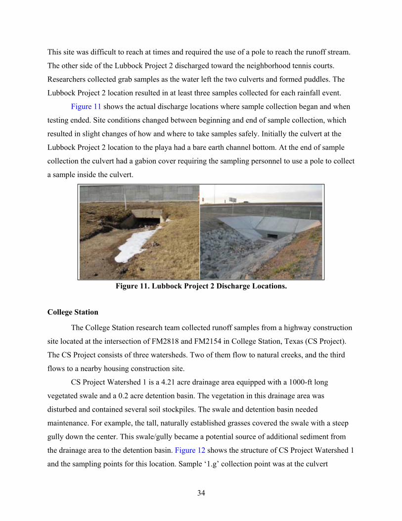
This site was difficult to reach at times and required the use of a pole to reach the runoff stream.
The other side of the Lubbock Project 2 discharged toward the neighborhood tennis courts.
Researchers collected grab samples as the water left the two culverts and formed puddles. The
Lubbock Project 2 location resulted in at least three samples collected for each rainfall event.
Figure 11 shows the actual discharge locations where sample collection began and when
testing ended. Site conditions changed between beginning and end of sample collection, which
resulted in slight changes of how and where to take samples safely. Initially the culvert at the
Lubbock Project 2 location to the playa had a bare earth channel bottom. At the end of sample
collection the culvert had a gabion cover requiring the sampling personnel to use a pole to collect
a sample inside the culvert.
Figure 11. Lubbock Project 2 Discharge Locations.
College Station
The College Station research team collected runoff samples from a highway construction
site located at the intersection of FM2818 and FM2154 in College Station, Texas (CS Project).
The CS Project consists of three watersheds. Two of them flow to natural creeks, and the third
flows to a nearby housing construction site.
CS Project Watershed 1 is a 4.21 acre drainage area equipped with a 1000-ft long
vegetated swale and a 0.2 acre detention basin. The vegetation in this drainage area was
disturbed and contained several soil stockpiles. The swale and detention basin needed
maintenance. For example, the tall, naturally established grasses covered the swale with a steep
gully down the center. This swale/gully became a potential source of additional sediment from
the drainage area to the detention basin. Figure 12 shows the structure of CS Project Watershed 1
and the sampling points for this location. Sample ‘1.g’ collection point was at the culvert

35
between the swale and the detention basin. Sample collection point ‘1’ is the discharge from the
detention basin toward the outside of the construction boundary. Figure 13 shows CS Project
Watershed 1 sampling points.
Figure 12. CS Project Watershed 1 Structure and Sampling Locations.
Figure 13. CS Project Watershed 1.
Left – Culvert and Detention Basin, Right – Discharge from the Detention Basin.
CS Project Watershed 2 is comprised of a 3.41 acre drainage area with a vegetated swale.
Figure 14 shows the structure of the watershed and turbidity values by sampling point.
Researchers collected samples at ‘2.f’ at the culvert to the swale and sample ‘2’ is the discharge
from the swale to adjacent creek. To see the influence of the discharge from the construction site
on the creek, the research team decided to collect samples before it mixed with the construction
site discharge (2.org) and the creek water after mixed (2.mix). However, researchers could not
collect ‘2.mix’ because of the unsafe field conditions. Figure 15 depicts the site conditions.
: space
: water sampling point

36
Figure 14. Structure of CS Project Watershed 2.
Figure 15. CS Project Watershed 2.
Left – Creek (before Construction Site Outlet) Where Water Is Already Turbid Right – Discharge from Construction Site to Creek.
Watershed 3 was comprised of two drainage areas and a vegetated swale with five silt
fences installed. The swale connects to a creek through a vegetated channel. The two drainage
areas in this watershed are relatively flat and well tilled. This makes the areas act like a detention
basin and can hold a large amount of rainfall runoff. However, the drainage areas release turbid
water once the rainfall volume exceeds the capacity due to the bare soil. See Figure 17 to Figure
19.
: space
: water sampling point

37
Figure 16. Structure of CS Project Watershed 3.
Figure 17. CS Project Watershed 3 Vegetated Channel and Discharge to Creek.
Figure 18. CS Project Watershed 3 Relatively Flat Drainage Area with Loose Bare Soil.
: space
: water sampling point

38
Figure 19. CS Project Watershed 3 Swale with Silt Fence on Bare Soil.
Hearne
The College Station research team collected runoff samples at the Highway 6 widening
project between Hearne and Calvert, Texas. The Hearne Project site is a 6-mile-long linear
project that crosses seven stream locations. The site had a paved road surface; however, the
roadside vegetation was not fully established. To separate the influence of the ongoing
construction site, researchers excluded the roadside section with fully vegetated cover. There
were five outlets selected for monitoring at this location.
One challenge in monitoring this site was the difficulty in separating and defining the net
influence of the construction site on stormwater discharge quality because the site contained
multiple drainage areas covering a far wider area than the project construction site. Researchers
selected five monitoring points for five outlets, but confirmed only two as originating from the
construction site.
Hearne Project Watershed 1 is a 10.8 acres linear-shape drainage area which has a
vegetated swale and a rock check dam. The swale is designed to discharge the stored water to
nearby grass field in the form of sheet flow, while, the outlet to stream is protected by a rock
check dam (Figure 20).

39
Figure 20. Hearne Project Watershed 1 Swale with Rock Check Dam.
Hearne Project Watershed 2 is a 501.6 acre drainage area that provides drainage beyond
the construction site boundary. Two channels merge and contribute to the final outlet in this
watershed. One is a concrete-paved channel from the construction site and the other is an
underground culvert from the outer construction site (Figure 21). A rock check dam exists near
the inlet of the concrete channel. Adjacent slopes have almost fully established vegetation except
some large bare soil surface areas.
Figure 21. Hearne Project Watershed 2 Concrete-Paved Channel.

40
Hearne Project Watershed 3 is a 36,368 acre natural drainage area that includes a major
creek. The creek is protected by a perimeter silt fence. The creek bank is a flat clay area with
sparse vegetation (see Figure 22).
Figure 22. Hearne Project Watershed 3 Turbid Natural Creek.
Hearne Project Watershed 4 has eight drainage areas that are linked together by a 5-mile
long swale fed by numerous culverts. The total area is approximately 260 acres. The swale is
covered by rock/concrete riprap (see Figure 23). This watershed includes a creek which typically
conveys water from adjacent 1,714 acres of natural drainage area; however, the creek remained
dry because of the lack of rainfall.

41
Figure 23. Hearne Project Watershed 4 Swale Covered by Rock Riprap.
Hearne Project Watershed 5 is 359.5 acres and serves an area much larger than the
construction site. A linear-shape swale following the road cuts across a natural creek in this
watershed. The swale is directly connected with the creek through culverts and holds water at all
times. The swale plays a role as a retention basin designed to discharge to an adjacent grass field
in the form of sheet flow. The outlet to stream is protected by a rock check dam (Figure 24).
Figure 24. Hearne Project Watershed 5 Swale Used as a Retention Basin.
Bryan
The Bryan Project study area was a lane expansion project for State Highway (SH) 47.
Researchers collected samples from six outlets in four sub-watersheds. Bryan Project Watershed
1 and 2 are located on the north side of the construction site. Both areas are linear shape swales
with a bare soil surface. Silt fence surrounded the site’s drop inlets (see Figure 25).

42
Figure 25. Bryan Project Watershed 1 on Left and Watershed 2 on Right.
Bryan Project Watershed 3 had a detention basin type of outlet with bare soil surface. The
outlet collects runoffs from both sides of the road construction site, and therefore has three
sampling points, including the collection point from each north and south side and the final outlet
toward the adjacent natural creek. The final outlet is blocked with silt fence, but the device is less
effective due to the large amount of concentrated water (see Figure 26). The researchers used an
automatic sampling system at the final outlet location.
Figure 26. Bryan Project Watershed 3 Collection Points.
Left – North Side, Middle – South Side, Right – Final Outlet and Detention Area.
Bryan Project Watershed 4 is located at the south side of the construction site as shown in
Figure 27. The area is a grassy channel slope. Runoff flows collected in this area were less turbid
due the vegetated surface. The outlet is connected to the adjacent private reservoir and had
multiple silt fences installed.

43
Figure 27. Bryan Project Watershed 4.
SAMPLING METHODS
Manual Sampling
The research team started collecting samples at the identified discharge locations after
rainfall events. When possible, samples of runoff leaving the project boundary were also
obtained. Whenever possible, researchers collected grab samples during the rain events. If the
rain ended, researcher obtained samples from the sedimentation pond with retained runoff. The
collection process was as follows:
Samples were collected downstream of the discharge location using a clean collection
bottle with the opening facing in the direction of the flow.
Care was taken to ensure the bottle did not overflow and the sampling site was not
disturbed by agitating particles upstream.
For low flows, a scoop was used to capture a sample so that the bottom settlements were
not disturbed, and for hard to reach locations, a pole was attached to a bottle to retrieve a
sample, both are recommendations from other state protocols (8).
A single grab sample from each sampling location was considered sufficient.
Automatic Sampling
Automatic sampling done at the Bryan Project used an ISCO 6712 sampler shown in
Figure 28. Samples were collected once every hour after activated at a certain level of runoff
flow. An ISCO 730 bubbler flow module was attached to the sampler and read flow depths once

44
every five minutes for selected rain events. The research team returned to the HSECL with the
samples to read their turbidities within 48 hours using the Hach 2100N turbidimeter used for the
grab samples.
Figure 28. ISCO 6712 Sampler and ISCO 730 Bubbler Flow Module.
Turbidity Measurements
Runoff sample analysis followed EPA method 180.1 with two modifications. The method
was developed for less turbid samples, i.e., drinking water, groundwater, etc., so the method
refers to a range of turbidity from 0 to 40 NTU. The first modification in the methodology was to
utilize this method using the Hach 2100N turbidimeter, which has a range of 0 to 4,000 NTU.
The samples were immediately transported to the lab, where they were analyzed for turbidity or
stored in the 4°C cold room to be analyzed within 7 days. This was the second modification to
the method as the methodology requires the analysis to be performed within 48 hours. Typically,
samples were analyzed within 48 hours, but for some sampling events, analysis was performed
after 48 hours. Therefore, a 7-day limit was utilized as the timeframe for sample analysis.
Researchers gently shook the samples and allowed the bubbles to dissipate prior to performing
the turbidity measurements.

45
RESULTS
Grab Sampling in Austin
Severe drought conditions have persisted in central Texas since September 2010, making
stormwater runoff sampling difficult. Over the three project sites, 15 samples were collected on
10 dates during the study period. As shown in Table 9, turbidity levels ranged from 35.5 to
> 4,000 NTU. Researchers collected samples from within the limits of construction. The
construction sites did not always discharge stormwater at the sampling time due to sediment
control practices, dry soil conditions, low rainfall intensities, and timing of sampling trips.
Management practices used on sampled areas of the construction project included silt
fencing and sedimentation ponds. Due to the limited number of samples, it is difficult to make
conclusions about the effectiveness of particular management practices. The data shows that the
turbidity varies based on rainfall intensity, duration of rainfall, amount of bare soil, best
management practices, and various other factors. The turbidity observations were consistent with
a previous study in the Austin area, which documented turbidity values ranging from 79 to
2,160 NTU in runoff from highway construction sites (13). Overall, the data suggests that the
runoff from construction sites is very turbid, and existing control practices may have difficulty
consistently meeting any new regulatory threshold that EPA and/or TCEQ may implement in the
future.
Table 9. Turbidity in Construction Site Runoff in Austin Area.
Austin Project 1 Austin Project 2 Austin Project 3 Date Rainfall
(mm) Turbidity
(NTU) Rainfall
(mm) Turbidity
(NTU) Rainfall
(mm) Turbidity
(NTU) 11/2/2010 4.3 2440.0 2.8 420.0 - -
1/15/2011 7.1 35.5 3.6 66.2 - - 1/15/2011 13.2 53.2 6.9 445.0 - - 5/12/2011 17.8 203.0 37.8 >4000 10.7 >4000 5/25/2011 - - - - 7.9 1256 6/22/2011 - - - - 34.8 >4000 10/8/2011 - - - - 6.9 >4000 10/9/2011 - - - - 48.5 >4000 11/8/2011 - - - - 4.8 565.0 11/15/2011 6.9 66.7 - - 6.6 1083.0

46
Grab Sampling in Lubbock
During the course of the study, four rainfall events occurred that allowed for sample
collection at both the Lubbock Project 1 at the Marsha Sharp Freeway and Lubbock Project 2 at
West Loop 289. March 4, May 11, and August 11, 2011 were the three days that samples were
obtained for both. Researchers collected one sample on July 12, 2011, at the Lubbock Project 1
location only. For the three times samples were collected at both sites, four total samples for each
rainfall event were collected—one at the Lubbock Project 1 location and three at the Lubbock
Project 2 location.
Turbidity values observed in the field ranged from 20 NTU up to around 10,600 NTU.
For all measurements the field turbidimeter read larger values than the lab turbidimeter. Table 10
shows a brief synopsis of the values read for each sample collected. The samples collected on
March 4th were not collected by the main operator on the project, therefore, the sample
collecting personnel did not have access to the field turbidimeter, and measurements were only
performed in the lab.
Table 10. Turbidity in Construction Site Runoff in Lubbock Area.
Turbidity (NTU) by Sampling Location
Date Lubbock Project 1
Lubbock Project 2
playa
Lubbock Project 2
small tennis
Lubbock Project 2
large tennis 3/4/2011 21.6 1889 252 60.2
5/11/2011 2205 601 226 49.0
7/12/2011 >4000* - - - 8/11/2011 4280 225 170 145 9/15/2011 235 32.2 22.9 238
* A dilution series was performed on this sample in the lab machine only and produced a final 10,600 NTU reading.
Grab Sampling in College Station
Samples from 12 rainfall events were collected in the CS Project site. Researchers
collected the first three samples during construction, the remaining after the road opened to the
public. The major difference between the two periods was the surface condition of drainage area.
Turbidity was reduced significantly in both outlets after an application of mulch on the roadside
surface even though vegetation was not yet established (see Table 11).

47
Table 11. CS Project Watersheds 1 and 2 Turbidities Readings of Samples. Date Rain
(inches) Sampling
Time Turbidity (NTU) Surface
Condition Watershed 1
Watershed 2
12/24/2010 0.66 raining 3903 - Disturbed bare soil 1/9/2011 1.69 1-hr later 860 833
1/16/2011 0.70 raining 1647 354 2/3/2012 4.11 6-hr later 12 56 Mulched
but no vegetation established
2/4/2012 2.15 1-hr later 51 68 2/10/2012 0.20 1-hr later N/F 52 2/13/2012 0.54 1-hr later 29 72 2/15/2012 0.45 1-hr later 82 129 2/18/2012 1.16 1-hr later 48 79 3/10/2012 2.62 3-hr later 4 17 3/20/2012 2.38 raining 13 61 3/29/2012 2.27 2-hr later 60 71
Note: N/F means “no flows” An interesting note is that the detention basin showed different performance by sampling
timing. Turbidity was reduced through the detention basin when collected after an hour
(1/9/2011), whereas, collection during rainfall events (12/24/2010 and 1/16/2011) showed
increased levels. This difference is probably due to the one hour interval allowing for
sedimentation to occur in the detention basin. During rainfall events, some of the sediment may
be redistributed within the basin and therefore discharge may be representative of this action.
Watershed 2 showed an improved turbidity level between the drainage area and the outlet
(from 354 to 143 NTU). Two reasons can be considered for this:
The swale condition.
The existence of a terraced vegetation basin.
Other watersheds of CS Project site showed that a swale or detention basin on bare soil
surface does not improve turbidity but becomes a source of additional sediments. This watershed
also had a bare soil swale adjacent to drainage area. However, the swale is not long and has a
flatter center line gradient so it was not expected to add as much sediment. Most of all, this
watershed was equipped with a high-performing sediment control method, a terraced vegetated

48
basin which was located between the upper swale and the lower creek. The terraced vegetated
area appeared able to:
Disperse the concentrated flow of the swale though the flat area.
Reduce the flow rate.
Capture sediments.
Table 12 shows turbidities in the CS Project Watershed 3. Runoff samples from the
drainage area ‘i’ show a large disparity in turbidity between two different rain events (i.e., 1338
NTU in the first event and 182 NTU in the second at the sample point ‘3.i’) even though the
surface conditions were almost consistent during that period. This is probably due to the
difference in precipitation volume, 1.69 inches for the first event and 0.7 inches for the second.
Table 12. CS Project Watershed 3 Turbidities of Samples.
Date Rain (inches)
Sampling Time
Turbidity (NTU) Surface Condition 3.h 3.i 3 3.mix 3.org
12/24/2010 0.66 raining 1334 Tilled bare
soil 1/9/2011 1.69 1-hr later 1863 1338 1991 163 142 1/16/2011 0.7 raining 197 182 358 75 67 2/3/2012 4.11 6-hr later 4 7 19 32 30
Mulched but no vegetation
2/4/2012 2.15 1-hr later 19.3 11 7 37 38 2/10/2012 0.20 1-hr later 6 8 N/F - - 2/13/2012 0.54 1-hr later 11 18 19 47 11 2/15/2012 0.45 1-hr later 44 25 73 80 30 2/18/2012 1.16 1-hr later 22 12 12 - - 3/10/2012 2.62 3-hr later 15 3 40 - - 3/20/2012 2.38 raining 37 20 11 - - 3/29/2012 2.27 2-hr later 15 7 5 104 36
The swale installed with five silt fences on bare soil surface did not help reduce turbidity.
The turbidity at the final outlet (‘3’ in Figure 28) in both rain events is greater than the turbidity
of discharge from the drainage area ‘3.h’ and ‘3.i’. This indicates that the series of swales is an
additional source of sediments at first glance. However, the turbidity of the accepting creek was
not changed much by the construction site discharge (e.g., 21 NTU from 142 to 163 NTU in the
first rain event). Silt fences in the swale held a large volume of water and discharged at the
significantly lower flow rate, thus the absolute amount of sediments per time may be lower at the
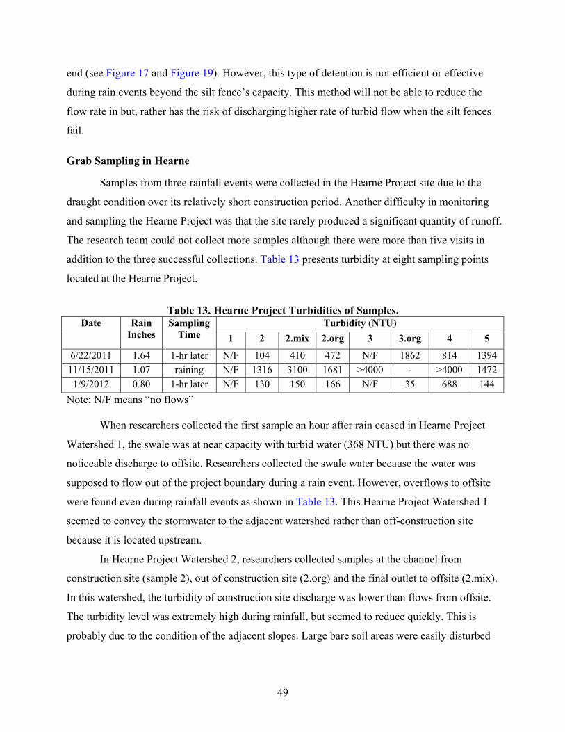
49
end (see Figure 17 and Figure 19). However, this type of detention is not efficient or effective
during rain events beyond the silt fence’s capacity. This method will not be able to reduce the
flow rate in but, rather has the risk of discharging higher rate of turbid flow when the silt fences
fail.
Grab Sampling in Hearne
Samples from three rainfall events were collected in the Hearne Project site due to the
draught condition over its relatively short construction period. Another difficulty in monitoring
and sampling the Hearne Project was that the site rarely produced a significant quantity of runoff.
The research team could not collect more samples although there were more than five visits in
addition to the three successful collections. Table 13 presents turbidity at eight sampling points
located at the Hearne Project.
Table 13. Hearne Project Turbidities of Samples.
Date Rain Inches
Sampling Time
Turbidity (NTU) 1 2 2.mix 2.org 3 3.org 4 5
6/22/2011 1.64 1-hr later N/F 104 410 472 N/F 1862 814 1394
11/15/2011 1.07 raining N/F 1316 3100 1681 >4000 - >4000 1472
1/9/2012 0.80 1-hr later N/F 130 150 166 N/F 35 688 144
Note: N/F means “no flows” When researchers collected the first sample an hour after rain ceased in Hearne Project
Watershed 1, the swale was at near capacity with turbid water (368 NTU) but there was no
noticeable discharge to offsite. Researchers collected the swale water because the water was
supposed to flow out of the project boundary during a rain event. However, overflows to offsite
were found even during rainfall events as shown in Table 13. This Hearne Project Watershed 1
seemed to convey the stormwater to the adjacent watershed rather than off-construction site
because it is located upstream.
In Hearne Project Watershed 2, researchers collected samples at the channel from
construction site (sample 2), out of construction site (2.org) and the final outlet to offsite (2.mix).
In this watershed, the turbidity of construction site discharge was lower than flows from offsite.
The turbidity level was extremely high during rainfall, but seemed to reduce quickly. This is
probably due to the condition of the adjacent slopes. Large bare soil areas were easily disturbed

50
during rainfall events; however, the sediments would settle down quickly to adjacent vegetated
areas after rainfall ceased.
Hearne Project Watershed 3 was the most environmentally sensitive area in the Hearne
site as the runoff from this watershed directly flowed to the nearby creek. Hearne Project
Watershed 3 had two sampling points—one at the outlet from the construction site (sample 3)
and the other from the natural creek (3.org). This watershed seems to develop a small amount of
stormwater flows to the outlet. Although the creek shore is located lower than adjacent half-
vegetated slopes, no noticeable ponding was found on the area even during a rainfall event.
There were no outflows from the small outlet under the silt fence when monitoring the site one
hour after rainfall ceased. Only a streak of outflow was found in the monitoring right after the
rainfall, but the turbidity was extremely high over 4000 NTU. The creek water showed various
turbidity levels (35 to 1862 NTU), which seemed to depend on rainfall intensity and volume.
Stormwater turbidities at the Hearne Project Watershed 4 were high, over 688, but
showed low flow rates during the monitoring period. The research team could not confirm if this
flow came from only the construction site or from another area. Hearne Project Watershed 5
seemed to be more affected by out-of-construction site conditions, and its turbidity level
appeared to be affected by rainfall characteristics. The samples collected on 1/9/2012 showed a
significantly lower turbidity when the rainfall had a lower intensity over a longer period of time.
Grab Sampling in Bryan
Samples from 11 rainfall events were collected in the Bryan Project site. Bryan Project
Watersheds 1 and 2 rarely produced any discharges. This may be due to the fact that their
drainage areas were large, flat, and pervious so most stormwater produced in the area was either
absorbed, infiltrated, or stored on-site. Bryan Project Watershed 3 produced very turbid runoff
levels due to discharges from the southbound area (“3.south” in Table 14). The southbound area
had disturbed bare soil conditions. While silt fence protected discharge from the area, it was
easily overtopped in the initial period (until 1/9/2013). The runoff from this area was
significantly reduced after the drainage area was flattened during construction. The Bryan
Project Watershed 4 had an established grass channel and produced minimal amounts of less
turbid water.

51
Table 14. Bryan Project Turbidities of Samples. Date Rain
(Inches) Sampling
Time Turbidity (NTU)
1 2 3.south 3.north 3 4 7/10/2012 0.09 1-hr later 334 116 N/F N/F N/F N/F 7/13/2012 1.84 1-hr later 277 106 N/F - 8400 209 12/27/2012 0.25 1-hr later N/F N/F N/F 144 314 N/F 1/4/2013 0.19 1-hr later N/F N/F 2068 99 254 46 1/8/2013 1.1 3-hr later N/F N/F N/F N/F 303 N/F
1/9/2013(1) 3 raining 649 N/F 5102 - 2829 239 1/9/2013(2) 3 raining - N/F 9017 - 4455 191
2/6/2013 raining N/F N/F N/F - 743 46 2/10/2013 raining 2907 5239 6558 - 2086 51 4/3/2013 1-hr later 779 N/F 218 - 792 N/F 4/19/2013 2-hr later N/F N/F N/F 127 238 35
Note: N/F means “no flows”
Automatic Sampling from Bryan
The Bryan Project successfully used automatic samplers for three rainfall events among
six attempts (see Figure 29–Figure 31). Results presented a wide variance in turbidity by the
discharge flow rate as shown in Table 15. The maximum turbidity reached 21,355 NTU in the
most intense rainfall event occurring on 1/9/2013. This implied that the time of grab sampling
would significantly change the turbidity estimate from a construction site.
Table 15. Bryan Project Turbidity Change by Time Using Data from Automatic Sampling.
Time (hr)
Turbidity by Date (NTU)
2/6/2013 2/18/2013 3/11/20130 743 777 23663 1 417 502 5987 2 347 3328 2103 3 215 1128 407 4 189 157 5 179 80 6 173 53 7 162 27
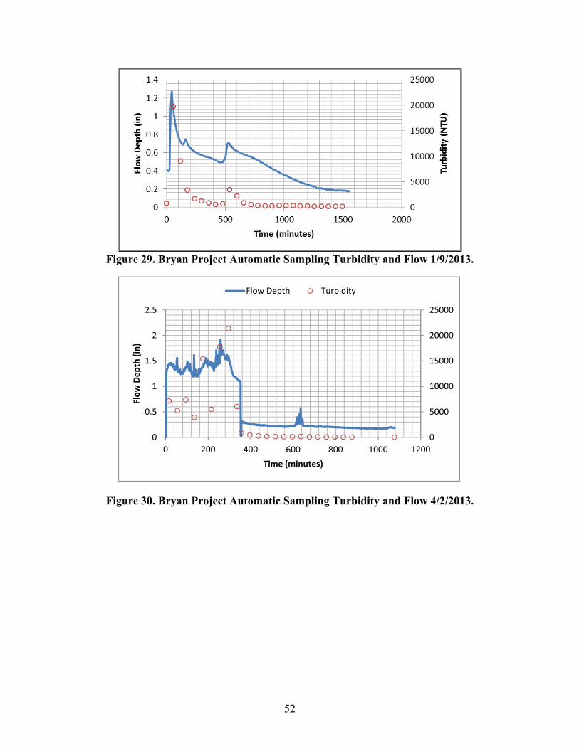
52
Figure 29. Bryan Project Automatic Sampling Turbidity and Flow 1/9/2013.
Figure 30. Bryan Project Automatic Sampling Turbidity and Flow 4/2/2013.
0
5000
10000
15000
20000
25000
0
0.5
1
1.5
2
2.5
0 200 400 600 800 1000 1200
Flow Depth (in)
Time (minutes)
Flow Depth Turbidity

53
Figure 31. Bryan Project Automatic Sampling Turbidity and Flow Depth 4/19/2013.


55
CONCLUSIONS AND FINDINGS
CONTROLLED TESTING OF COAGULANTS
Polyacrylamide for Erosion Control
The PAM application used in this evaluation was not effective in significantly reducing
turbidity or soil loss on clay soils with 1:3 slopes. Maximum turbidities of all tested ECB
treatments were very high, ranging from 3,450 to 9,037 NTU. The turbidity of the effluent from
the bare soil plot reached 52,857 NTU. Average dry soil losses overall agreed with turbidity
results.
Due to the high range of turbidity the efficiency of PAM could not be determined.
Although PAM showed a lower turbidity and average dry soil loss on bare soil and excelsior
ECB than untreated counterparts, the differences were negligible. Furthermore, when applied
with jute and straw erosion control blankets the reduction in turbidity decreased. This result was
unexpected because straw ECBs are typically considered excellent performers in a 1:3 clay soil
application. These results are shown in Table 16 and Table 17.
Table 16. Maximum Turbidity from Controlled Erosion Control Tests. Surface Condition No PAM
Treated PAM Treated Difference
Bare soil 52,857 NTU 51,987 NTU -870 Jute ECB over 4,040* NTU over 4,040* NTU NA
Excelsior ECB 3,603 NTU 3,450 NTU -153 Straw ECB 4,180 NTU 9,037 NTU +4,857
* exceeds the capacity of the Hach SOLITAX in situ turbidity sensor
Table 17. Average Dry Soil Loss from Controlled Erosion Control Tests.
Surface Condition No PAM Treated PAM Treated Difference
Bare soil 175.50 lb 163.10 lb -12.40 Jute ECB 17.25 lb 19.05 lb +1.80
Excelsior ECB 6.97 lb 5.43 lb -1.54 Straw ECB 0.40 lb 10.17 lb +9.77
Several potential reasons could contribute to the test results. First, broadcast application
might limit the efficacy of PAM. The PAM2 hand-broadcasted on jute ECB did not develop any
visible flocculation during the tests; as a result, the dry soil loss of its effluent was equivalent

56
with the untreated jute ECB. Meanwhile, the PAM1 applied with the hydroseeder on the straw
ECB created highly viscous flocculation from the soil surface to the discharge outlet. It is
speculated that those flocculated sediments adhered inside the straw ECB, but in reality the
sediment clogs appeared too heavy to be held on the blanket’s surface, particularly when using
the heavy design storm of 3.5 inches per hour. Also, the PAM1 appeared to facilitate more
flocculation by softening the surface soil. This was most likely due to the high viscosity caused
by the application of PAM1.
Polyacrylamide for Sediment Control
To compare the sediment removal efficiency of treated and untreated sediment retention
devices, wood fiber wattles were installed in SRD test flume. Mass loading of the outflow was
estimated using flow rate and turbidity monitored at the one minute resolution. The following
data was recorded and calculated to determine removal efficiency:
Flow-through rate (cfs).
Maximum flow rate (gpm).
Ponding volume (gal).
Turbidity at inlet and outlet (NTU).
SSC (mg/L) at inlet and outlet.
Mass loading (lb).
Removal efficiency (%).
Test results demonstrated that PAM treated sediment control devices were significantly
more successful at reducing sediment from sediment laden water than untreated SRDs. The
removal efficiencies of PAM treated wattles ranged from 8 percent to 18 percent improvement.
Table 18 shows these results.

57
Table 18. Sediment Removal Efficiency of Untreated and PAM Treated Wattles.
Sediment Retention Device
Test Roun
d
Mass In lb (kg)
Mass Out lb (kg)
Removal Efficiency%
Wattle – untreated 1 1.3 (0.58) 0.69 (0.31) 46 2 1.4 (0.65) 0.79 (0.36) 45 3 1.6 (0.71) 0.85 (0.39) 46
Wattle – PAM treated 1 1.47 (0.67) 0.54 (0.24) 63 2 1.54 (0.70) 0.61 (0.28) 61 3 1.47 (1.47) 0.67 (0.30) 54
Coagulation and Dosing of Polyacrylamides
The flocculation tests were performed to understand the soil characteristics, polymer
characteristics, and doses that promote flocculation. Researchers generated turbidity curves as a
function of polymer dose added for each modified synthetic stormwater runoff. Comparison of
these curves and the soil characteristics gives insight about the interactions between the PAM
and the particles in the modified synthetic stormwater runoff.
Interparticle bridging is commonly accepted as the mechanism by which PAM interacts
with soils to destabilize particles. Since particles are negatively charged, they repel one another.
Interparticle bridging may overcome this repulsion if the polymer is able to span the distance
between two particles, thereby forming a floc. The polymer’s ability to bridge two particles is
referred to as its grappling distance and is a function of its molecular weight. The higher the
molecular weight of the polymer, the longer it’s grappling distance. Therefore, flocculants with
higher molecular weights are expected to be more effective at promoting flocculation due to their
improved ability to bridge particles.
Figure 32 shows the turbidity curves for the modified synthetic stormwater runoff of
WLoop soil for the polymers P-21, A-110, and A-110 HMW. The objective of these tests was to
determine how molecular weight effects turbidity reduction. PAM P-21 is clearly ineffective at
reducing the turbidity. It also had the lowest molecular weight of 0.2 Mg mol-1 indicating a
minimum grappling distance to effectively bridge particles in the suspension may exist. A-110
had a higher molecular weight of 10-12 Mg mol-1 and was effective at reducing the turbidity
below 280 NTU. A-110 HMW had a molecular weight of 10-14 Mg mol-1 and has a similar
turbidity curve to A-110. This result is expected since A-110 and A-110 HMW have a similar

58
range of molecular weights. However, A-110 HMW was observed to be more viscous than A-
110 when working with these polymers during the experiments. The greater viscosity indicates
that A-110 HMW does have a higher molecular weight than A-110, since viscosity is a surrogate
measure for the molecular weight. The similar turbidity curves of A-110 and A-110 HMW
support the concept that a minimum molecular weight may be required to promote interparticle
bridging. The similarity also implies a plateau effect may exist, where an increase in molecular
weight above 10 Mg mol-1 does not increase the effectiveness of the anionic PAMs.
Figure 32. Impact of Molecular Weight on Turbidity Reduction for Modified Synthetic
Stormwater Runoff for WLoop Soil.
The effect of charge density on flocculation is shown in Figure 33. The non-ionic PAM,
SF N300, is the most effective polymer. A-110, which has a charge density of 16 percent, is less
effective than the non-ionic PAM, but is more effective than A-150, which has the highest
charge density of 50 percent. The turbidity curves clearly indicate that as charge density
increased, the effectiveness of PAM decreased. This trend occurred in all the synthetic runoff
samples that were tested. Intuitively, this trend is expected. The particles are negatively charged;
therefore, the addition of an anionic PAM would increase the negative charge on the particle
surfaces, making them more difficult to flocculate. Flocculation will occur if the grappling
distance of the PAM is able to overcome these repulsive forces. The addition of a non-ionic
0
200
400
600
800
1000
1200
1400
1600
1800
2000
0.01 0.1 1 10
Tur
bidi
ty (N
TU
)
Dose (mg/L)
Init Turbidity
Control
Threshold
P-21
A-110
A-110 HMW

59
PAM, however, does not increase the charge of the particles and therefore it would be expected
to be the most effective.
Figure 33. Effect of Charge Density on Flocculation for Modified Synthetic Stormwater
Runoff Using Wloop Soil.
Furthermore, Figure 33 shows a difference between the optimal dose of anionic PAMs
and non-ionic PAMs. The optimal dose for SF N300 was 10 mg/L (see Appendix B) compared
to the optimal dose for the anionic PAMs of 3 mg/L. The optimal dose for the anionic PAMs and
the non-ionic PAMs varied between 1-3 mg/L and 10 mg/L, respectively, for all the synthetic
runoff tested. Their study observed the optimal dose for anionic PAMs was lower than those of
non-ionic PAMs for kaolinite suspensions. The lower optimal dose was a result of the anionic
PAMs’ ability to form loops and tails due to their anionic charge, while the non-ionic polymer
was not able to form these loops and tails. Figure 32 demonstrates that the optimal dose for
anionic PAM is lower than that of non-ionic PAM for synthetic runoff.
Figure 34 shows the polymers that were most effective in reducing the turbidity of the
synthetic runoff was WLoop. The non-ionic PAMs, SF N300, and LMW SF N300, reduced the
turbidity to 20 and 55 NTU, respectively. The molecular weight of these PAMs was 15 and 6 Mg
mol-1, respectively. SF N300, with its higher molecular weight, was more effective than the
LMW SF N300 for all the runoff tested. This confirms the previous trend found with anionic
0
200
400
600
800
1000
1200
1400
1600
1800
2000
0.01 0.1 1 10
Tur
bidi
ty (N
TU
)
Dose (mg/L)
Init Turbidity
Control
Threshold
SF N300
A-110
A-150

60
PAMs, which indicated that higher molecular weights are more effective to a certain threshold.
APS #705 was also effective at promoting flocculation and reduced the turbidity to 23 NTU at its
optimal dose. The turbidity curve of APS #705 was nearly identical to the curve of SF N300
indicating APS #705 may have similar charge characteristics to the non-ionic PAM.
Furthermore, the flocs created by APS #705 were similar to all the PAMs in that they were
“fluffy.” These fluffy flocs are indicative of interparticle bridging. The flocs formed by chitosan
were denser. The denser flocs are expected to be observed as the mechanism of particle
destabilization with chitosan is a combination of charge neutralization and interparticle bridging.
Figure 34. Most Effective Flocculants for Modified Synthetic Stormwater Runoff Wloop.
The optimal dose of chitosan was 3 mg/L, beyond which restabilization occurred. The
optimal dose associated with chitosan depends on its mechanism of particle destabilization.
When charge neutralization is the dominant mechanism of particle destabilization, the optimal
dose will be the dose at which the zeta potential is zero. The cationic polymer will adsorb to the
surfaces of the particle, which neutralizes the charge of the particle until it is zero.
Restabilization will occur when the adsorption of chitosan to the particles causes the particles to
have a net positive charge, thereby causing particles to repel one another. When interparticle
bridging is the dominant mechanism of particle destabilization, overdosing of chitosan will be
the same as overdosing with PAM. Restabilization will occur when the adsorption sites on the
0
200
400
600
800
1000
1200
1400
1600
1800
2000
0.01 0.1 1 10 100
Tur
bidi
ty (N
TU
)
Dose (mg/L)
Init Turbidity
Control
Threshold
SF N300
LMW SF N300
APS #705
Chitosan

61
particle are saturated by chitosan to the extent that flocs are prevented from forming. The optimal
dose of chitosan was found to range from 1 to 10 mg/L for all the synthetic runoff tested, which
indicates the mechanism of particle destabilization may be different for the various samples of
synthetic runoff.
Restabilization of the non-ionic PAMs and APS #705 is a result of overdosing the
synthetic runoff, which is the same restabilization that occurs for chitosan when interparticle
bridging is its mechanism of particle destabilization. Researchers observed the restabilization of
the non-ionic PAMs and APS #705 for all the synthetic runoff tested beyond the optimal dose of
10 mg/L. The non-ionic PAMs, APS #705, and chitosan were the most effective at promoting
flocculation for all the synthetic runoff tested. In particular, SF N300, APS #705, and chitosan
reduced the turbidity of the synthetic runoff below 280 NTU for all the synthetic runoff tested.
The LMW SF N300 reduced the turbidity below 280 NTU for all but one synthetic runoff, E.
Texas soil, and was the lease effective of these four polymers.


63
REFERENCES
1. US Environmental Protection Agency, Office of Water (4303T). November 2009.
Development Document for Final Effluent Guidelines and Standards for the Construction &
Development Category. Washington, D.C.
2. US Small Business Administration. 2013. Construction and Development Effluent
Limitations Guidelines - Proposed Rule. http://www.sba.gov/advocacy/820/593731.
3. National Association of Home Builders. 2013. NAHB v. U.S. EPA (Effluent Limitation
Guidelines). http://www.nahb.org/generic.aspx?genericContentID=135750.
4. Ma, J.S., J.H. Kang, M. Kayhanian, and M.K. Stenstrom. 2009. Sampling issues in urban
runoff monitoring programs: Composite versus grab. Journal of Environmental Engineering,
135:118-127.
5. Harmel, R.D., K.W. King, and R.M. Slade. 2003. Automated storm water sampling on small
watersheds. Applied Engineering in Agriculture, 19:667-674.
6. Campbell, C., D. Laycak, W. Hoppes, N. Tran, and F. Shi. May 2006. High concentration
suspended sediment measurements using a continuous fiber optic in-stream transmissometer.
Journal of Hydrology; Volume 311, Issue 1 – 4.
7. Kayhanian, M., K. Murphy, L. Regenmorter, and R. Haller. 2001. Characteristics of storm-
water runoff from highway construction sites in California. Transportation Research Record:
Journal of the Transportation Research Board 1743, no. 1 (January 1): 33-40.
doi:10.3141/1743-05.
8. McLaughlin, R. 2002. Measures to Reduce Erosion and Turbidity in Construction Site
Runoff. Technical Report. Washington, D.C.: U.S. Department of Transportation.
9. McLaughlin, R. and G. Jennings. 2007. Minimizing Water Quality Impacts of Road
Construction Projects. Technical Report. Raleigh, NC: North Carolina State University.
10. California State Water Resources Control Board Division of Water Quality. 2009.
http://www.swrcb.ca.gov/water_issues/programs/stormwater/docs/construction/2009_0009_d
wq_nel_amnd.pdf.
11. Washington State, Department of Ecology. 2006. How to do Stormwater Sampling: A Guide
for Construction Sites. Publication #06-10-020.

64
12. Oregon Department of Environmental Quality. 2005. General Permit National Pollutant
Discharge Elimination System Stormwater Discharge Permit State Permit 1200-C.
http://www.deq.state.or.us/wq/stormwater/constappl.htm.
13. Barrett, M., J. Kearney, T. McCoy, and J. Malina. 1995. An Evaluation of the Performance of
Temporary Sediment Controls. Center for Water Resources, The University of Texas at
Austin. http://www.crwr.utexas.edu/reports/pdf/1995/rpt95-6.pdf.

65
BIBLIOGRAPHY
Barnett, A. P., E. G. Diseker and E. C. Richardson. 1967. Evaluation of Mulching Methods for
Erosion Control on Newly Prepared and Seeded Highway Backslopes. Agronomy Journal
59:83-85.
Benik, S.R., B.N.Wilson, D.D. Biesboer, B. Hansen and D. Stenlund. 2003. Evaluation of
erosion control products using natural rainfall events. Journal of Soil and Water
Conservation 58(2):98-104.
Flanagan, D.C., K. Chaudhari and L.D. Norton. 2002. Polyacrylamide soil amendment effects on
runoff and sediment yield on steep slopes: Part 1. Simulated rainfall conditions. Transactions of
the American Society of Agricultural Engineers 45(5): 1327-1337.
King, B.A., B. Izadi, MS. Ashraf, R.H. Brooks and W.H. Neibling. 1996. On-farm comparison
of polyacrylamide and straw mulch on dry bean yields, irrigation performance and erosion.
University of Idaho Publication No. 101-96, pp.5559.
Lentz, RD., I. Shainberg, R.E. Sojka and D.L. Carter. 1992. Preventing irrigation furrow erosion
with small applications of polymers. American Journal of Soil Science. 56:1926-1932.
Roa-Espinosa,A., G.D. Bubenzer and E.S. Miyashita. 1999. Sediment and runoff control on
construction sites using four application methods of polyacrylamide mix. American Society of
Agricultural Engineers, Paper No.99-2013, American Society of Agricultural Engineers, St.
Joseph, Michigan.
Roa, A. 1996. Screening of Polymers to Determine Their Potential Use in Erosion Control on
Construction Sites, University of Idaho Publication No. 101-96, pp.77-83.
Wallace,G.A. and A.Wallace. 1986. Control of soil erosion by polymeric soil conditioners. Soil
Science Journal, 141(5):363-367.


67
APPENDIX A: STATE NUMERIC STANDARDS FOR CONSTRUCTION SITES
State Numeric Effluent Standards for Active Construction Sites
Alabama
No statewide standard but 2011 ALR 100000 CGP requires construction site monitoring and sampling for turbidity. Alabama Department of Environmental Management. 2011. National Pollution Discharge Elimination System General Permit ALR 100000. http://www.adem.alabama.gov/programs/water/waterforms/ALR10CGP.pdf.
Alaska
No statewide standard Alaska Department of Environmental Conservation. 2011. Alaska Pollutant Discharge Elimination System General Permit for Discharges from Large and Small Construction Activities AKR 100000. http://dec.alaska.gov/water/wnpspc/stormwater/docs/Final_2011_ACGP_(20110519)_w_app.pdf.
Arizona
No statewide standard. Arizona Department of Environmental Quality. Arizona Pollutant Discharge Elimination System General Permit for Stormwater Discharges Associated with Construction Activity to Waters of the United States. June 2013. http://www.azdeq.gov/environ/water/permits/download/2013_cgp.pdf.
Arkansas
No statewide standard - 80% removal of TSS from post-construction only. Arkansas Department of Environmental Quality. General Permit No. ARR150000. http://www.adeq.state.ar.us/water/branch_permits/general_permits/stormwater/construction/pdfs/ARR150000_permit.pdf
California
Draft Construction General Permit includes turbidity levels of 1,000 NTU. If Active Treatment Systems are used, a daily average of 10 NTUs is noted. California State Water Resources Control Board, Division of Water Quality. 2010. National Pollutant Discharge Elimination System General Permit for Storm Water Discharges Associated With Construction and Land Disturbance Activities, CAS000002. http://www.swrcb.ca.gov/board_decisions/adopted_orders/water_quality/2012/wqo2012_0006_dwq.pdf.
Colorado
No statewide standard. Colorado Department of Public Health and Environment. 2007. CDPS General Permit Stormwater Discharges Associated With Construction Activity, Permit No. COR-030000. http://www.cicacenter.org/pdf/copermit.pdf=1251808459293&ssbinary=true.
Connecticut No numeric standard. Turbidity monitoring required at least once a month during construction activity if there is discharge.

68
State Numeric Effluent Standards for Active Construction Sites Connecticut Department of Energy and Environmental Protection. General Permit for the Discharge of Stormwater and Dewatering Wastewaters from Construction Activities. 2013. http://www.ct.gov/deep/lib/deep/permits_and_licenses/water_discharge_general_permits/storm_construct_gp.pdf. Accessed 2013.
Delaware
No statewide standard. Delaware Department of Natural Resources and Environmental Control. http://www.dnrec.delaware.gov/swc/Pages/SedimentStormwater.aspx. Accessed 2013.
Florida
No statewide standard. State of Florida, Department of Environmental Protection. Generic Permit for Stormwater Discharge from Large and Small Construction Activities. 2009. http://www.dep.state.fl.us/water/stormwater/npdes/docs/cgp.pdf. Accessed 2011.
Georgia
New CGPs GAR100001 and GAR100002, effective 9-2013, require site monitoring and sampling. Georgia Environmental Protection Department of Natural Resources. 2013. NPDES General Permit No. GAR100001 for Stand Alone Construction Projects and NPDES General Permit No. GAR100002 for Infrastructure Construction Projects. http://www.gaepd.org/npdes/. Accessed 2013.
Hawaii
No statewide standard. Hawaii Department of Health. NPDES General Permit Authorizing Discharges of storm Water Associated with Construction Activity. 2007. http://health.hawaii.gov/cwb/files/2013/04/HAR1155.pdf.
Idaho
No statewide standard. Uses EPA CGP. Idaho Department of Environmental Quality http://www.deq.state.id.us/permitting/water-quality-permitting/npdes.aspx. Accessed 2013.
Illinois
No statewide standard Illinois Environmental Protection Agency, Division of Water Pollution Control. 2013. National Pollutant Discharge Elimination System General NPDES Permit For Storm Water Discharges From Construction Site Activities, General NPDES Permit No.ILR10. http://www.epa.state.il.us/water/permits/storm-water/general-construction-permit.pdf. Accessed 2013.

69
State Numeric Effluent Standards for Active Construction Sites
Indiana
No statewide standard. Indiana Department of Environmental Management. Article 15. NPDES General Permit Rule Program. 1996. http://www.in.gov/idem/4902.htm.
Iowa
No statewide standard - 80% removal of TSS from post-construction only. Iowa Department of Natural Resources. 2007. NPDES General Permit No. 2 for Storm Water Discharge Associated with Industrial Activity for Construction Activities. http://www.iowadnr.gov/portals/idnr/uploads/water/stormwater/guidanceno2.pdf. Accessed 2011.
Kansas
No statewide standard. Kansas Department of Health and Environment. Kansas Water Pollution Control and National Pollutant Discharge Elimination System Stormwater Runoff From Construction Activities General Permit. 2012. http://www.kdheks.gov/stormwater/download/Const%20SW%20Issued%203-2-2012%20Packet.pdf. Accessed 2013.
Kentucky
No statewide standard - 80% TSS reduction compared to pre-construction levels. Kentucky Energy and Environment Cabinet. 2009. Kentucky Pollutant Discharge Elimination System (KPDES) General Permit For Stormwater Discharges Associated With Construction Activities (KYR10). http://water.ky.gov/permitting/General%20Permit%20Fact%20Sheets/FinalPermitKYR10000RTC_2_.pdf. Accessed 2011.
Louisiana
No statewide standards related to construction sites. Louisiana Department of Environmental Quality. 2009. General Permit for Discharge of Storm Water from Construction Activities Five (5) Acres of More, LAR100000. http://www.deq.louisiana.gov/portal/Portals/0/permits/lpdes/pdf/FINAL%20LAR100000.pdf. Accessed 2011.
Maine
No statewide standard. Maine Department of environmental Protection. 2006. General Permit – Construction Activity Maine Pollutant Discharge Elimination System (MPDES). http://www.maine.gov/dep/land/stormwater/2006mcgp.pdf. Accessed 2011.

70
State Numeric Effluent Standards for Active Construction Sites
Maryland
No statewide standard. Maryland Department of the Environment.2009. General Permit for Stormwater Associated with Construction Activity. http://www.mde.maryland.gov/programs/Permits/WaterManagementPermits/WaterDischargePermitApplications/Documents/2014GP-FactSheet.pdf. Accessed 2013.
Massachusetts
No statewide standard-uses EPA Construction General Permit. Massachusetts Energy and Environmental Affairs. http://www.mass.gov/eea/agencies/massdep/water/wastewater/stormwater.html#4. Accessed 2011.
Michigan
No statewide standard. Michigan Department of Environmental Quality. http://www.michigan.gov/deq/0,4561,7-135-3313_3682_3716---,00.html. Accessed 2013.
Minnesota
No statewide standard. Minnesota Pollution Control Agency. 2013. General Permit Authorization to Discharge Stormwater Associated With Construction Activity under the National Pollutant Discharge Elimination System/State Disposal System Program, Permit No. MN R 100001. http://www.pca.state.mn.us/index.php/view-document.html?gid=18984. Accessed 2013.
Mississippi
No statewide standard; however, has ACT9 (LCGP) Optional Monitoring, which was changed to optional due to changes in C&G Rule. Mississippi Department of Environmental Quality Office of Pollution Control. 2011. Large Construction General Permit. http://www.deq.state.ms.us/MDEQ.nsf/pdf/epd_ConstructionStormWaterGeneralPermit(5acresandgreater)/$File/05General.pdf. Accessed 2013.
Missouri
The effluent limitation for Settleable Solids from a stormwater outfall discharging shall not exceed 2.5 ml/L per Standard Method 2540 F, except immediately following the local 2-year, 24-hour storm event. The Settleable Solids limit is not enforceable during or greater that the local 2-year, 24-hour storm event. Missouri Department of Natural Resources. Missouri State Operating Permit, General Operating Permit MORA00000. 2012. http://www.dnr.mo.gov/env/wpp/permits/issued/RA00000.pdf. Accessed 2013.

71
State Numeric Effluent Standards for Active Construction Sites
Montana
No statewide standard. Montana Department of Environmental Quality. 2012. General Permit for Storm Water Discharges Associated with Construction Activity. http://www.deq.mt.gov/wqinfo/MPDES/StormwaterConstruction.mcpx. Accessed 2013.
Nebraska
No statewide standard. Nebraska Department of Environmental Quality. 2008. Authorization to Discharge Under the National Pollutant Discharge Elimination System (NPDES) General NPDES Permit Number NER110000 for Storm Water Discharges from Construction Sites to Waters of the State of Nebraska. http://www.transportation.nebraska.gov/letting/Forms/NPDES%20General%20Permit.pdf. Accessed 2013.
Nevada
No statewide standard. Nevada Department of Conservation & Natural Resources. 2007. Stormwater General Permit NVR 100000. http://ndep.nv.gov/docs_07/nvr100000_permit07.pdf. Accessed 2013.
New Hampshire
No statewide standard. New Hampshire. 2012. EPA National Pollutant Discharge Elimination System General Permit for Discharges from Construction Activities. http://www.epa.gov/npdes/pubs/cgp2012_finalpermit.pdf. Accessed 2013.
New Jersey
No statewide standard – post-construction standard only. New Jersey Department of Environmental Protection. Permit to Discharge Stormwater from Construction into the Surface Waters of the State of New Jersey. 2011. http://www.state.nj.us/dep/dwq/pdf/5g3_factsheet.pdf. Accessed 2011.
New Mexico
No statewide standard. New Mexico. 2012. EPA National Pollutant Discharge Elimination System General Permit for Discharges from Construction Activities. http://www.epa.gov/npdes/pubs/cgp2012_finalpermit.pdf. Accessed 2013.
New York
No statewide standard. New York State Department of Environmental Conservation. 2010. SPDES General Permit for Stormwater Discharges from Construction Activity. http://www.dec.ny.gov/docs/water_pdf/gpsconspmt10.pdf. Accessed 2011.

72
State Numeric Effluent Standards for Active Construction Sites
North Carolina
No statewide standard. North Carolina Department of Environment and Natural Resources Division of Water Quality. 2006. General Permit to Discharge Stormwater under the National Pollutant Discharge Elimination System. http://cicacenter.org/pdf/ncpermit.pdf Accessed 2011.
North Dakota
No statewide standard. North Dakota Department of Health. 2009. Authorization to Discharge under the North Dakota Pollutant Discharge Elimination System. http://www.ndhealth.gov/WQ/Storm/Construction/NDR10per20091001F.pdf Accessed 2011.
Ohio
No statewide standard. Ohio Department of Natural Resources. 2013. General Permit Authorization for Storm Water Discharges Associated with Construction Activity under the National Pollutant Discharge Elimination System. http://www.epa.ohio.gov/Portals/35/permits/OHC000004_GP_Final.pdf. Accessed 2013.
Oklahoma
No statewide standard. Oklahoma Department of Environmental Quality – Water Quality Division. 2012. General Permit OKR10 for Stormwater Discharges from Construction Activities Within the State of Oklahoma. http://www.deq.state.or.us/wq/wqpermit/docs/general/npdes1200c/permit.pdf. Accessed 2013.
Oregon
No statewide standard. Oregon Department of Environmental Quality. 2010. General Permit – National Pollutant Discharge Elimination System Stormwater Discharge Permit. http://www.deq.state.or.us/wq/wqpermit/docs/general/npdes1200c/permit.pdf. Accessed 2011.
Pennsylvania
No statewide standard. Pennsylvania Department of Environmental Protection. 2010. General Permit for Coverage Under General NPDES Permit For Stormwater Discharges Associated with Construction Activities. http://www.elibrary.dep.state.pa.us/dsweb/Get/Document-91750/3150-PM-BWEW0280%20Fact%20Sheet.pdf . Accessed 2011.
Rhode Island
No statewide standard – post-construction standard only. Rhode Island Department of Environmental Management. 2013. General Permit for Stormwater Discharge Associated with Construction Activity. http://www.dem.ri.gov/pubs/regs/regs/water/ripdesca.pdf. Accessed 2013.

73
State Numeric Effluent Standards for Active Construction Sites
So. Carolina
No statewide standard. South Carolina Department of Health & Environmental Control. 2012. NPDES General Permit for Stormwater Discharges from Construction Activities. http://www.scdhec.gov/environment/water/swater/docs/CGP-permit.pdf. Accessed 2013.
So. Dakota
No statewide standard. South Dakota Department of Environment and Natural Resources. 2010. General Permit for Storm Water Discharges Associated with Construction Activities. http://denr.sd.gov/des/sw/IPermits/ConstructionGeneralPermit2010.pdf. Accessed 2011.
Tennessee
No statewide standard. Tennessee Department of Environment & Conservation. 2011. General NPDES Permit for Discharges of Stormwater Associated with Construction Activities (Permit No. TNR100000). http://www.tennessee.gov/environment/water/docs/wpc/tnr100000.pdf. Accessed 2011.
Texas
No statewide standard - concrete batch plants only. Texas Commission on Environmental Quality. 2013. General Permit to Discharge Under the Texas Pollutant Discharge Elimination System (Permit No. TXR105000). http://www.tceq.texas.gov/assets/public/permitting/stormwater/TXR150000_CGP.pdf. Accessed 2013.
Utah
No statewide standard. Utah Department of Environmental Quality Division of Water Quality. 2010. Storm Water General Permit for Construction Activities. Permit No. UTR300000. http://www.waterquality.utah.gov/UPDES/docs/2008/07Jul/GeneralConstructionPermiUTR3000000t.pdf. Accessed 2011.
Vermont
2008 Construction General Permit notes a 25 NTU limit for moderate-risk sites. Vermont Agency of Natural Resources. 2008. General Permit for Stormwater Runoff from Construction Sites. http://www.anr.state.vt.us/dec/waterq/stormwater/docs/construction/sw_cgp_amended_final.pdf. Accessed 2011.

74
State Numeric Effluent Standards for Active Construction Sites
Virginia
No statewide standard. Virginia Department of Environmental Quality. 2009. General Permit for Discharges of Stormwater from Construction Activities. http://www.deq.virginia.gov/Portals/0/DEQ/Water/Publications/CGPvar10.pdf. Accessed 2011.
Washington
Turbidity shall not exceed 5 NTU over background turbidity when the background turbidity is 50 NTU or less, or has more than a 10 percent increase in turbidity when the background turbidity is more than 50 NTU. Washington State Department of Ecology. 2010. National Pollutant Discharge Elimination System (NPDES) and State Waste Discharge General Permit for Stormwater Discharges Associated with Construction Activity. http://www.ecy.wa.gov/programs/wq/stormwater/construction/permitdocs/cswgppermit120110.pdf Accessed 2011.
West Virginia
No statewide standard. West Virginia Department of Environmental Protection. 2012. State of West Virginia Department of Environmental Protection Division of Water and Waste Management. http://www.dep.wv.gov/WWE/Programs/stormwater/csw/Documents/Final_Signed_2012_CSW_General_Permit.pdf. Accessed 2013.
Wisconsin
Construction sites must implement erosion and sediment controls to reduce to the maximum extent practicable 80% of the annual sediment load. Wisconsin Department of Natural Resources. 2011. Wisconsin Pollutant Discharge Elimination System General Permit for Construction Site Storm Water Runoff. http://dnr.wi.gov/topic/stormwater/documents/fact_sheet_wi-s067831-4_sept_2011.pdf. Accessed 2011.
Wyoming
No statewide standard. Wyoming Department of Environmental Quality. 2011. General Permit to Discharge Storm Water Associated with Construction Activity Under the Wyoming Pollutant Discharge Elimination System (WYPDES). http://deq.state.wy.us/wqd/wypdes_permitting/wypdes_storm_water/downloads/LCGP_2011_final.pdf. Accessed 2011.

75
APPENDIX B: TYPICAL RUNOFF TURBIDITY FOR ROAD CONSTRUCTION PROJECTS FROM PREVIOUS STUDIES
Source Construction
Type Location
State Sampling
Year Runoff Turbidity
Remark Min Max Mean Kayhanian et al. (7)
Roadway / Highway
CA 1998-2000 15 16000 702 15 sites
McLaughlin (8)
1:2 fill slope NC 2001 50 5600 1638 PAM 1:2 fill slope NC 2001 25 4000 634 PAM+mulch+seed1:4 cut slope NC 2001 200 5900 2272 PAM 1:4 cut slope NC 2001 50 400 182 PAM+mulch+seed1:4 fill slope NC 2001 11 2000 360 PAM 1:4 fill slope NC 2001 18 500 116 PAM+mulch+seed
McLaughlin and Jennings (9)
Highway NC 2004-2005 77 28160 2950 Final outlet Highway NC 2004-2006 6 18223 1647 Final outlet Highway NC 2004-2007 6 2272 159 Final outlet Highway NC 2004-2008 3 9409 1178 Final outlet
