performance of multistep finite control set model...

IEEE TRANSACTIONS ON POWER ELECTRONICS, VOL. 30, NO. 3, MARCH 2015 1633

Performance of Multistep Finite Control Set ModelPredictive Control for Power Electronics

Tobias Geyer, Senior Member, IEEE, and Daniel E. Quevedo, Senior Member, IEEE

Abstract—The performance of direct model predictive control(MPC) with reference tracking and long prediction horizons isevaluated through simulations, using the current control problemof a variable speed drive system with a voltage source inverter as anillustrative example. A modified sphere decoding algorithm is usedto efficiently solve the optimization problem underlying MPC forlong horizons. For a horizon of five and a three-level inverter, forexample, the computational burden is reduced by four orders ofmagnitude, compared to the standard exhaustive search approach.This paper illustrates the performance gains that are achievable byusing prediction horizons larger than one. Specifically, for long pre-diction horizons and a low switching frequency, the total harmonicdistortion of the current is significantly lower than for space vectormodulation, making direct MPC with long horizons an attractiveand computationally viable control scheme.

Index Terms—Branch and bound, drive systems, finite controlset, model predictive control (MPC), power electronics, quantiza-tion, sphere decoding.

I. INTRODUCTION

THE optimization problem underlying direct (also calledfinite control set) model predictive control (MPC) with ref-

erence tracking is typically solved by enumerating all possiblesolutions [2]. Since the number of possible solutions increasesexponentially as a function of the length of the prediction hori-zon, when using enumeration, enlarging the prediction horizonentails an exponential increase in the computation time. Fordirect MPC with reference tracking, this combinatorial explo-sion has to date, in effect, limited the length of implementableprediction horizons to one [3], [4]. Conversely, solving the opti-mization problem of direct MPC with long prediction horizonsin an efficient manner has been hitherto an unresolved problem.

A solution approach to this problem is proposed in [5], whichadopts the notion of sphere decoding [6] and tailors it to theproblem at hand. As a result, the optimization problem under-

Manuscript received June 6, 2013; revised October 6, 2013, February 16,2014, and accepted April 3, 2014. Date of publication April 8, 2014; date ofcurrent version October 15, 2014. This work was supported under AustralianResearch Council’s Discovery Projects funding scheme (project number DP110103074). The work of T. Geyer was supported by a grant from ABB Cor-porate Research, Switzerland, while being with the University of Auckland,New Zealand. The material in this paper was presented at the IEEE EnergyConversion Congress and Exposition (ECCE) 2013 in Denver, CO, USA, see[1]. Recommended for publication by Associate Editor G. Escobar.

T. Geyer is with the ABB Corporate Research, Baden-Dattwil 5405,Switzerland (e-mail: [email protected]).

D. E. Quevedo is with the University of Newcastle, Newcastle, NSW 2308,Australia (e-mail: [email protected]).

Color versions of one or more of the figures in this paper are available onlineat http://ieeexplore.ieee.org.

Digital Object Identifier 10.1109/TPEL.2014.2316173

lying MPC with long prediction horizons, such as ten, can besolved, using enumeration, on average as quickly as the horizonof one case.

In this paper, we start by summarizing the problem formu-lation and the key results obtained in [5]. Using a three-levelneutral point clamped (NPC) voltage source inverter driving aninduction machine as a case study, we present a detailed per-formance evaluation that highlights essential features of directMPC with horizons significantly longer than one by using theoptimization algorithm presented in [5]. At steady-state operat-ing conditions, the key performance metrics are the total har-monic distortion (THD) of the current and the device switchingfrequency. Several comparisons with two commonly used mod-ulation schemes are performed, i.e., space vector modulation(SVM) and optimized pulse patterns (OPPs) [7], [8]. Interest-ingly, in some cases MPC with long horizons has the potentialto achieve a performance similar to that of OPPs, even at steadystate. During transients, MPC with long horizons provides atransient response time as short as MPC with short horizons,often outperforming classic control arrangements such as fieldoriented control.

II. CONTROL PROBLEM AND SOLUTION METHOD

This section recapitulates the main subject matter of [5], bysummarizing the control problem, MPC formulation, and theefficient solution method based on sphere decoding.

A. Control Problem

In the stationary αβ coordinate system, we consider adiscrete-time linear power electronic system modeled as per

x(k + 1) = A x(k) + B uαβ (k) (1a)

y(k) = C x(k) (1b)

with system matrices A, B, and C, and k ∈ N. We use uαβ =P u with

P =23

[1 − 1

2 − 12

0√

32 −

√3

2

](2)

to translate the three-phase switch positions u � [ua ub uc ]T

into the orthogonal coordinate system. Note that u ∈ U3 is in-teger valued. For a three-level inverter, for example, we haveU = {−1, 0, 1}. For a drive system with an induction machine,we choose as state vector x � [isα isβ ψrα ψrβ ]T , whereis � [isα isβ ]T denotes the stator current, and ψrα and ψrβ arethe rotor flux linkages. The system output is chosen as y = is .

0885-8993 © 2014 IEEE. Personal use is permitted, but republication/redistribution requires IEEE permission.See http://www.ieee.org/publications standards/publications/rights/index.html for more information.

1634 IEEE TRANSACTIONS ON POWER ELECTRONICS, VOL. 30, NO. 3, MARCH 2015

The control problem is to regulate the stator current along itsreference i∗s , by manipulating the three-phase switch positionu. The switching effort, i.e., the switching frequency or theswitching losses is to be kept small.

B. Model Predictive Control Formulation

The cost function

J =k+N −1∑

�=k

‖ie,αβ (� + 1)‖22 + λu‖Δu(�)‖2

2 (3)

is a suitable choice to penalize the predicted evolution of thecurrent errors and the control effort over the prediction horizonof N steps, where

ie,αβ (� + 1) � i∗s,αβ (� + 1) − is,αβ (� + 1) (4a)

Δu(�) � u(�) − u(� − 1) . (4b)

The scalar parameter λu ≥ 0 is a tuning parameter that adjuststhe tradeoff between the tracking accuracy and the switchingeffort.

Introducing the switching sequence U(k) =[uT (k) . . . uT (k + N − 1)]T , the optimization problemunderlying direct MPC with current reference tracking is

U opt(k) = arg minU(k) J (5a)

subject to U(k) ∈ U (5b)

‖Δu(�)‖∞ ≤ 1, ∀� = k, . . . , k + N − 1, (5c)

where U = U3N . The constraint (5c) is imposed since switchingis only possible by one step up or down in each phase.

C. Efficient Method for Calculating the OptimalSwitch Positions

Using algebraic manipulations, the optimization problem (5)can be rewritten as

U opt(k) = arg minU(k) ‖Uunc(k) − HU(k)‖22 (6a)

subject to (5b) and (5c). (6b)

H turns out to be an invertible lower triangular matrix, see [5].We use U unc(k) � HUunc(k), where Uunc(k) is the switchingsequence obtained from minimizing (5) without constraints, i.e.,with U = R3N and ignoring (5c).

The MPC optimization problem in its form (6) is a (trun-cated) integer least-squares problem. As shown in [5], thesphere decoding algorithm [6], [9] can be adapted to solve (6).The algorithm iteratively considers candidate sequences U ∈ Uwithin a sphere of radius ρ(k) > 0 centered in Uunc(k), i.e.,‖Uunc(k) − HU‖2 ≤ ρ(k), and which satisfy the switchingconstraint (5c). Since H is triangular, finding candidate se-quences is computationally simple, in the sense that at each steponly a one-dimension problem needs to be solved. For moredetails, the reader is referred to [5] and [6].

Fig. 1. Three-level three-phase neutral point clamped voltage source inverterdriving an induction motor with a fixed neutral point potential.

TABLE IRATED VALUES (LEFT) AND PARAMETERS (RIGHT) OF THE DRIVE

III. FRAMEWORK FOR PERFORMANCE EVALUATION

A. Case Study

We consider a NPC voltage source inverter connected with amedium-voltage induction machine and a constant mechanicalload, as shown in Fig. 1. A 3.3 kV and 50 Hz squirrel-cage in-duction machine rated at 2 MVA with a total leakage inductanceof 0.25 pu is used as an example of a typical medium-voltageinduction machine. The dc-link voltage is Vdc = 5.2 kV andassumed to be constant. The potential of the neutral point N isassumed to be fixed. The detailed parameters of the machine andinverter are summarized in Table I. The per unit (pu) system is es-tablished using the base quantities VB =

√2/3Vrat = 2694 V,

IB =√

2Irat = 503.5 A, and fB = frat = 50 Hz, with Vrat ,Irat , and frat referring to the rated voltage, current, and fre-quency, respectively.

All simulations are performed in MATLAB, using an ideal-ized setup with the semiconductors switching instantaneously.As such, second-order effects such as deadtimes, controller com-putation delays, measurement noise, observer errors, saturationof the machine’s magnetic material, parameter variations, etc.,are neglected, resulting in a switched linear model for the drivesystem. The significance of such simulations is underlined bythe very close match between previous simulations and exper-imental results using a similar model. The simulation resultsin [10] predicted the experimental results in [11] accurately towithin a few percent. Throughout this paper, if not otherwisestated, all simulations were done at nominal speed and ratedtorque, implying a fundamental frequency of 50 Hz and ratedcurrents. All results are shown in the pu system.

GEYER AND QUEVEDO: PERFORMANCE OF MULTISTEP FINITE CONTROL SET MODEL PREDICTIVE CONTROL FOR POWER ELECTRONICS 1635

B. Modulation Methods Used for Benchmarking

To evaluate the steady-state performance of multistep optimaldirect MPC, we benchmark this strategy with SVM and OPPs.The SVM gating signals are obtained by using a three-levelregular sampled PWM with two triangular carrier signals, whichare in phase (phase disposition). By adding to the referencevoltage an appropriate common mode voltage, which is of themin/max plus modulo type, the modulator resembles a SVM, asshown in [12]. Synchronous modulation is used, i.e., the carrierfrequency is an integer multiple of the fundamental frequency.

The OPPs were calculated offline for pulse numbers (ratio be-tween the switching frequency and the fundamental frequency)of up to 15. The switching angles were computed by minimizingthe squared differential-mode voltage harmonics divided by theorder of the harmonic. For an inductive load such as a machine,this approach is effectively equivalent to minimizing the currentTHD [8].

C. Performance Criteria

The key criteria related to the control performance are thedevice switching frequency fsw and the current THD ITHD . Inaddition, we will also investigate the a posteriori closed-loopcost. It is obtained after the simulations, by evaluating the costfunction J from (3) over all simulated time-steps and dividingit by the total number of time-steps ktot

Jcl =1

ktot

k t o t−1∑�=0

‖ie,αβ (� + 1)‖22 + λu‖Δu(�)‖2

2 . (7)

In summary, the closed-loop cost (7) captures the squared rmscurrent error plus the weighted averaged and squared switchingeffort over the closed-loop simulation.

D. Trade-Off Between Current THD and Switching Frequency

Unavoidably, with switching power converters, there is atradeoff between the current THD ITHD and the switching fre-quency fsw . It is convenient to plot these two quantities alongtwo orthogonal axes. Fig. 2 illustrates this performance tradeofffor SVM and OPPs. In the figure, each square corresponds toa unique simulation with synchronous SVM. The squares areapproximated using a polynomial, indicated by the dash-dottedline. Accordingly, the diamonds correspond to steady-state sim-ulations with OPPs.

The switching frequency range between 200 and 350 Hz isof particular importance for medium-voltage power converters.As can be seen in Fig. 2, in the given range, there is scope fora significant reduction of the current THD, while maintainingthe same switching frequency. For example, at fsw = 200 Hzthe current THD can be almost halved, when replacing SVMby OPPs. Conversely, the switching frequency can be drasti-cally reduced for the same current THD. For ITHD = 5%, forexample, the switching frequency can be lowered from 350 to200 Hz, when adopting OPPs instead of SVM. This is a reduc-tion of 42%. Both examples are indicated by red arrows shownin Fig. 2.

Fig. 2. Tradeoff between the current THD ITHD and the switching frequencyfsw for synchronous space vector modulation (SVM) and optimized pulsepatterns (OPPs).

At high switching frequencies, however, the performancebenefit of OPPs compared to SVM tends to be marginal. Forfsw > 600 Hz and pulse numbers greater than 12, the differenceis very small. Moreover, the optimization process to computeOPPs with very high pulse numbers becomes computationallydemanding and the memory space required to store such pat-terns is significant. As a result, we have computed OPPs only upto pulse number 15, or equivalently, up to a switching frequencyof 750 Hz.

With the above as a background and recalling that OPPsexhibit, to a large extent, optimal steady-state behavior, we willquantify in the sequel the relative merits of MPC by normalizingthe current THD to the one obtained by OPPs. Specifically, weintroduce

δTHD =ITHD − ITHD ,OPP

ITHD ,OPP(8)

which is the relative current THD degradation, normalized to thecurrent THD of OPPs and given in percent. The normalization isdone with regard to the polynomial approximation of the OPPsshown in Fig. 2. For switching frequencies beyond 750 Hz,SVM is used as a baseline, since OPPs were computed only upto this frequency.

IV. STEADY-STATE PERFORMANCE

In this section, the performance of direct MPC with long pre-diction horizons is investigated at steady-state operating condi-tions, using the three-level inverter with an induction machineas a case study. We use the modified sphere decoding algorithmdescribed in [5] to solve the optimization problem. To ensurethat the drive system has settled at steady-state operating con-ditions, the system is first simulated over several fundamentalperiods without recording the results.

A. Comparison at 250-Hz Switching Frequency

Consider direct MPC with the horizon of N = 1, samplinginterval Ts = 125μs, and cost function (3) with the weighting


Fig. 3. Simulated waveforms for direct MPC with the horizon of N = 1, sampling interval Ts = 125 μs and weighting λu = 8.4 · 10−3 , at full speed and ratedtorque. The switching frequency is approximately 250 Hz. (a) Stator currents is . (b) Stator current spectrum. (c) Switch positions u.

TABLE IICOMPARISON OF DIRECT MPC WITH SVM AND AN OPP IN TERMS OF THE

CURRENT THD ITHD , TORQUE THD TTHD , SWITCHING FREQUENCY fsw ,AND SWITCHING LOSSES Psw . THE PENALTY λu , CARRIER FREQUENCY fc ,

AND PULSE NUMBER d ARE CHOSEN SUCH THAT A SWITCHING FREQUENCY OF

APPROXIMATELY 250-HZ RESULTS

factor λu = 8.4 · 10−3 . This results in an average device switch-ing frequency of fsw = 250 Hz, which is typical for medium-voltage applications, and a current THD of ITHD = 5.96%.

Fig. 3(a) illustrates three-phase stator current waveformsalong with their (dash dotted) references over one fundamentalperiod. The colors blue, green, and red correspond to the phasesa, b, and c, respectively. The evolution of the stator current issimulated with a time resolution of 25μs, based on which thespectrum of the stator current is computed with a Fourier trans-formation. The resulting current spectrum is shown in Fig. 3(b)and the three-phase switching sequence is depicted in Fig. 3(c).For direct MPC, unlike PWM, a repetitive switching pattern isnot enforced. As a result, the current spectrum is predominatelyflat without characteristic harmonics, despite a pronounced 11thharmonic.

Extending the prediction horizon to N = 10 reduces the cur-rent THD by about one percentage point, as stated in Table II.This first result indicates that long prediction horizons do in-deed reduce the current THD, in this case by about 15%. Thecorresponding waveforms for the N = 10 case are shown inFig. 4. It can be seen that the long horizon leads to a certaindegree of repetitiveness in the switching pattern. Accordingly,nontriplen odd-order harmonics are clearly identifiable in thecurrent spectrum, such as the 11th, 13th, and 19th harmonics.Indeed, the degree of repetitiveness in the switching patternand, correspondingly, the magnitude of the discrete harmonicsin the current spectrum are remarkable. It can be observed that,in this case, long prediction horizons foster a discrete current

spectrum, by concentrating the harmonic power in harmonics ofodd order. An analysis shows that the same applies to the triplen(common mode) voltage harmonics. The shift of some of theharmonic ripple power into common mode harmonics is oneof the reasons, why direct MPC with long prediction horizonsleads, in general, to a lower current THD than the horizon of onecase. Moreover, longer horizons result in a shift of some of thedifferential-model voltage harmonics from the low-frequencyrange to higher frequencies, resulting in a lower current THD.

To facilitate a comparison with SVM, the correspondingwaveforms of SVM are shown in Fig. 5. The equivalent car-rier frequency fc = 450 Hz results in the same switching fre-quency as for MPC, i.e., fsw = 250 Hz. The current THDis at 7.71% significantly higher than with direct MPC, seeTable II. As expected, due to the symmetry and repetitiveness ofthe switching pattern, SVM features a discrete current spectrumwith distinctive harmonics at nontriplen and odd multiples ofthe fundamental frequency. Note that the 17th current harmonichas an amplitude of 0.066.

On the other hand, for the same switching frequency and thepulse number d = 5, an OPP leads to a current THD of 4.12%,which is approximately one percentage point lower than fordirect MPC with N = 10.

B. Closed-Loop Cost

Next, the influence of λu on the switching frequency, the cur-rent THD, and the closed-loop cost in (7) is investigated. Foreach of the horizons N = 1, 3, 5, and 10 and for more than1000 different values of λu , ranging between 0 and 0.5, steady-state simulations were run. Focusing on switching frequenciesbetween 100 Hz and 1 kHz, and current THDs below 20%, theresults are shown in Fig. 6, using a double logarithmic scale.Each simulation corresponds to a single data point. Polyno-mial functions are overlaid, which approximate the individualdata points. Figs. 6(a) and (b) suggest that, for small predictionhorizons, the relationship between λu and the performance vari-ables is approximately linear in the double logarithmic scale; forlarger values of N , the relationship is more complicated, but stillmonotonic.

When extending the horizon for a given λu , the switchingfrequency is increased, while the current THD is significantly


Fig. 4. Simulated waveforms for direct MPC with the horizon of N = 10, sampling interval Ts = 125 μs and weighting λu = 8.3 · 10−3 . The operating pointand the switching frequency are the same as in Fig. 3. (a) Stator currents is . (b) Stator current spectrum. (c) Switch positions u.

Fig. 5. Simulated waveforms for SVM with the equivalent carrier frequency fc = 450 Hz. The operating point and the switching frequency are the same as inFig. 3. (a) Stator currents is . (b) Stator current spectrum. (c) Switch positions u.

Fig. 6. Key performance criteria of MPC for the prediction horizons N = 1, 3, 5, 10 and sampling interval Ts = 25 μs. The switching frequency, current THDand closed-loop cost are shown as a function of the tuning parameter λu , using a double logarithmic scaling. The individual simulations are indicated using dots,their overall trend is approximated using dash-dotted polynomials. (a) Average switching frequency fsw . (b) Current THD ITHD . (c) Closed-loop cost Jcl .

reduced. This waterbed effect makes it difficult to assess fromFigs. 6(a) and (b) the benefit long prediction horizons mighthave on these two key performance metrics. A more suitablemeasure is the a posteriori closed-loop cost, see (7), which isillustrated in Fig. 6(c). As the prediction horizon is increasedthe cost is clearly reduced, suggesting the use of horizons largerthan one. For example, with λu = 0.01 and N = 1, we haveJcl ≈ 0.05, whereas with the horizon of N = 3, the closed-loop cost can be reduced to Jcl ≈ 0.003. This is a reductionby a factor of 17! We also note that, for this value of λu , theachieved a posteriori closed-loop cost is almost optimal. The

benefit of long horizons on the current THD and the switchingfrequency is investigated in the subsequent sections, see alsoFigs. 7–11. For guidelines about how to tune λu please also referto [13].

C. Relative Current THD for Sampling Interval Ts = 25μs

Fig. 7 shows the relative current THDs of SVM and of MPC,as defined in (8). In this figure, the simulations referring toSVM are indicated by squares, those of OPPs are indicated withdiamonds. Using the sampling interval Ts = 25μs, hundreds ofindividual simulations of MPC with prediction horizons N =


fsw (Hz)(a)

fsw (Hz)(b)

fsw (Hz)(c)

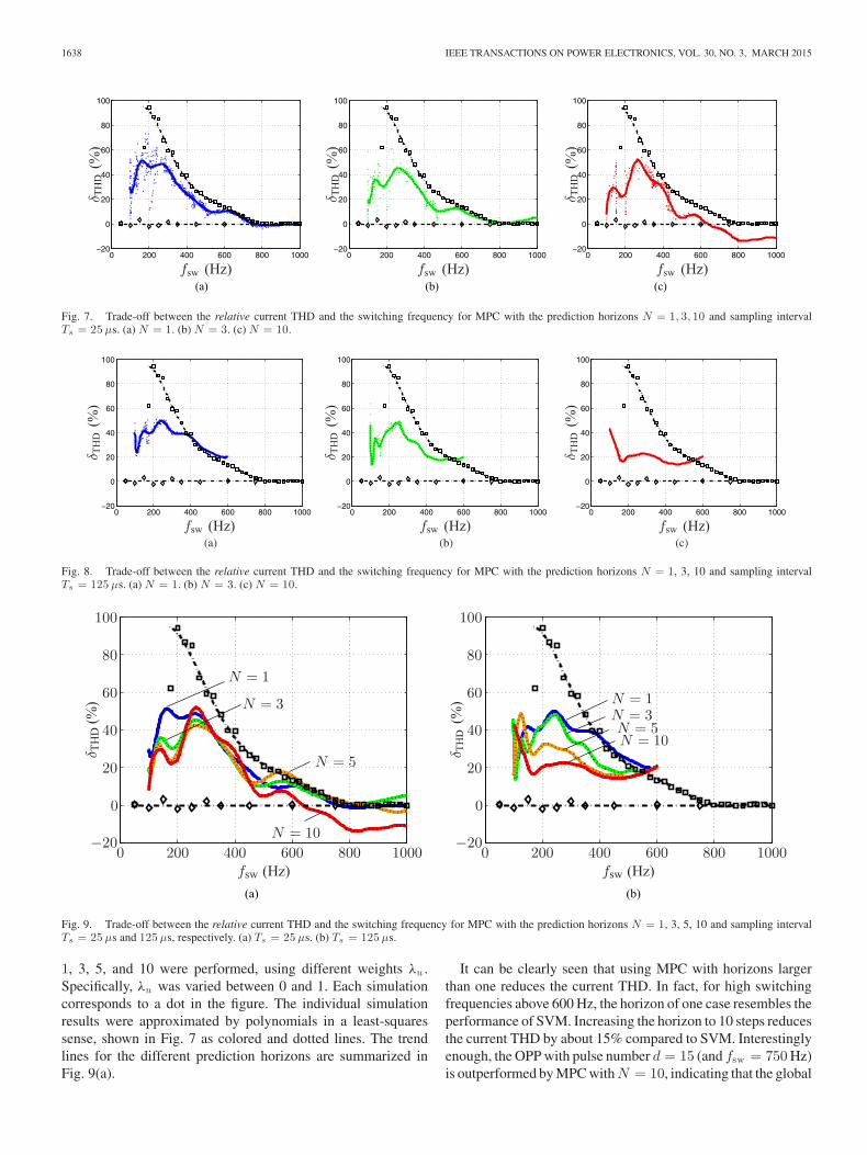
Fig. 7. Trade-off between the relative current THD and the switching frequency for MPC with the prediction horizons N = 1, 3, 10 and sampling intervalTs = 25 μs. (a) N = 1. (b) N = 3. (c) N = 10.

Fig. 8. Trade-off between the relative current THD and the switching frequency for MPC with the prediction horizons N = 1, 3, 10 and sampling intervalTs = 125 μs. (a) N = 1. (b) N = 3. (c) N = 10.

(a) (b)

Fig. 9. Trade-off between the relative current THD and the switching frequency for MPC with the prediction horizons N = 1, 3, 5, 10 and sampling intervalTs = 25 μs and 125 μs, respectively. (a) Ts = 25 μs. (b) Ts = 125 μs.

1, 3, 5, and 10 were performed, using different weights λu .Specifically, λu was varied between 0 and 1. Each simulationcorresponds to a dot in the figure. The individual simulationresults were approximated by polynomials in a least-squaressense, shown in Fig. 7 as colored and dotted lines. The trendlines for the different prediction horizons are summarized inFig. 9(a).

It can be clearly seen that using MPC with horizons largerthan one reduces the current THD. In fact, for high switchingfrequencies above 600 Hz, the horizon of one case resembles theperformance of SVM. Increasing the horizon to 10 steps reducesthe current THD by about 15% compared to SVM. Interestinglyenough, the OPP with pulse number d = 15 (and fsw = 750 Hz)is outperformed by MPC with N = 10, indicating that the global


Fig. 10. Trade-off between the relative current THD and the switching frequency for MPC with the prediction horizons N = 1, 3, 10, using Monte Carlosimulations. (a) N = 1. (b) N = 3. (c) N = 10.

minimum was not obtained when computing this particular OPP.In absolute terms, however, the differences are small, being inthe range of a fraction of a percent (in terms of the absolutecurrent THD).

For low switching frequencies between 100 and 250 Hz, theperformance results are somewhat scattered. The trend lines sug-gest that around fsw = 200 Hz the current THD can be reducedby about 30%, when increasing the prediction horizon fromN = 1 to 5. Longer horizons do not appear to carry any addi-tional performance benefit. Interestingly, for long horizons suchas N = 10 and low switching frequencies, the switching fre-quency appears to lock into integer multiples of the fundamen-tal frequency. This is apparent for fsw = 100, 150, and 200 Hz.For these switching frequencies and for particular choices of λu ,MPC almost reproduces the steady-state performance of OPPs,in terms of the current THD achieved for a given switchingfrequency.

D. Relative Current THD for Sampling Interval Ts = 125μs

The simulations shown in the previous section are repeatedhere for a five times longer sampling interval, i.e., Ts = 125μs.Fig. 8 shows the resulting trade-off relations, analog to thosein Fig. 7. The summary plot is provided in Fig. 9(b). As in theTs = 25μs case, longer prediction horizons improve the perfor-mance of MPC by lowering the current THD for a given switch-ing frequency. This becomes particularly evident for switchingfrequencies between 150 and 450 Hz. In this range, MPC withN = 10 exhibits a relative current THD that is approximately20% lower than that for the N = 1 case. When comparing Figs.9(a) and (b), we note that in addition to the weight λu , thechoice of sampling interval has a significant impact on the re-sulting closed-loop performance. This somewhat complicatesthe tuning procedure of direct MPC.

All trade-off curves converge at fsw = 600 Hz, which corre-sponds to a zero penalty on the switching effort, i.e., λu = 0.When not penalizing the switching transitions and thus onlypenalizing the predicted deviation of the current from its sinu-soidal reference, MPC turns into a deadbeat controller. Here,the current loop effectively constitutes two first-order systems(one in the α- and another one in the β-axis) and the length ofthe prediction horizon ceases to have an impact on the perfor-

Fig. 11. Trade-off between the relative current THD and the switching fre-quency for MPC with the prediction horizons N = 1, 3, 5, 10, using MonteCarlo simulations.

mance of MPC. In this situation, MPC with N = 1 yields thesame control action as MPC with N > 1, compare this also tothe results in [14] and [15].

E. Relative Current THD for Monte Carlo Simulations

We have seen that, in addition to the tuning parameter λu

and the horizon N , the sampling interval Ts has a profoundinfluence on the MPC performance. The reason for this is thatthe MPC cost function in (3) evaluates system predictions overa prediction horizon of length NTs in time.

To derive results that take into account a variety of sam-pling intervals, we carried out Monte Carlo simulations withrandom sampling intervals and random weights. Specifically,the sampling interval was randomly chosen from the intervalTs ∈ [5, 200]μs, and the weight was chosen from λu ∈ [0, 5].Moreover, the initial conditions of the drive system are random,including random initial stator currents and rotor fluxes for theinduction machine, and random initial switch positions for theinverter. As previously, to ensure the simulations to be capturedat steady state, presimulations were run that were not recorded.

MPC with prediction horizons N ∈ {1, 3, 5, 10} was consid-ered and approximately 104 simulations were performed. The


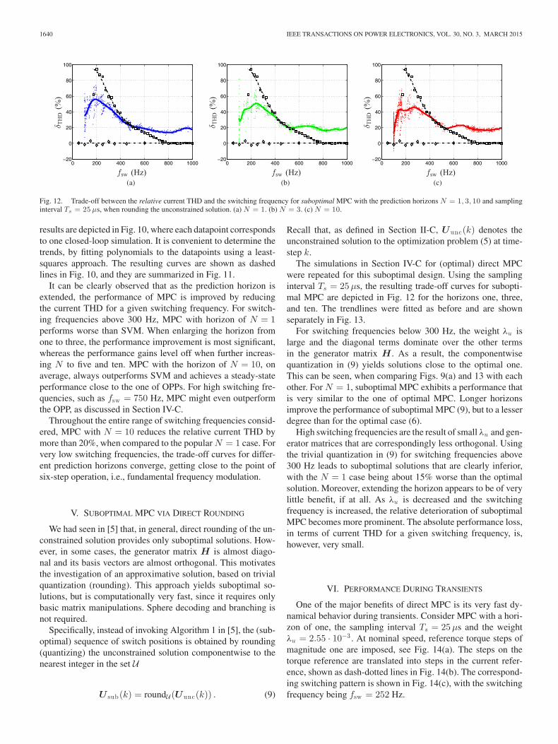
Fig. 12. Trade-off between the relative current THD and the switching frequency for suboptimal MPC with the prediction horizons N = 1, 3, 10 and samplinginterval Ts = 25 μs, when rounding the unconstrained solution. (a) N = 1. (b) N = 3. (c) N = 10.

results are depicted in Fig. 10, where each datapoint correspondsto one closed-loop simulation. It is convenient to determine thetrends, by fitting polynomials to the datapoints using a least-squares approach. The resulting curves are shown as dashedlines in Fig. 10, and they are summarized in Fig. 11.

It can be clearly observed that as the prediction horizon isextended, the performance of MPC is improved by reducingthe current THD for a given switching frequency. For switch-ing frequencies above 300 Hz, MPC with horizon of N = 1performs worse than SVM. When enlarging the horizon fromone to three, the performance improvement is most significant,whereas the performance gains level off when further increas-ing N to five and ten. MPC with the horizon of N = 10, onaverage, always outperforms SVM and achieves a steady-stateperformance close to the one of OPPs. For high switching fre-quencies, such as fsw = 750 Hz, MPC might even outperformthe OPP, as discussed in Section IV-C.

Throughout the entire range of switching frequencies consid-ered, MPC with N = 10 reduces the relative current THD bymore than 20%, when compared to the popular N = 1 case. Forvery low switching frequencies, the trade-off curves for differ-ent prediction horizons converge, getting close to the point ofsix-step operation, i.e., fundamental frequency modulation.

V. SUBOPTIMAL MPC VIA DIRECT ROUNDING

We had seen in [5] that, in general, direct rounding of the un-constrained solution provides only suboptimal solutions. How-ever, in some cases, the generator matrix H is almost diago-nal and its basis vectors are almost orthogonal. This motivatesthe investigation of an approximative solution, based on trivialquantization (rounding). This approach yields suboptimal so-lutions, but is computationally very fast, since it requires onlybasic matrix manipulations. Sphere decoding and branching isnot required.

Specifically, instead of invoking Algorithm 1 in [5], the (sub-optimal) sequence of switch positions is obtained by rounding(quantizing) the unconstrained solution componentwise to thenearest integer in the set U

U sub(k) = roundU (Uunc(k)) . (9)

Recall that, as defined in Section II-C, Uunc(k) denotes theunconstrained solution to the optimization problem (5) at time-step k.

The simulations in Section IV-C for (optimal) direct MPCwere repeated for this suboptimal design. Using the samplinginterval Ts = 25μs, the resulting trade-off curves for subopti-mal MPC are depicted in Fig. 12 for the horizons one, three,and ten. The trendlines were fitted as before and are shownseparately in Fig. 13.

For switching frequencies below 300 Hz, the weight λu islarge and the diagonal terms dominate over the other termsin the generator matrix H . As a result, the componentwisequantization in (9) yields solutions close to the optimal one.This can be seen, when comparing Figs. 9(a) and 13 with eachother. For N = 1, suboptimal MPC exhibits a performance thatis very similar to the one of optimal MPC. Longer horizonsimprove the performance of suboptimal MPC (9), but to a lesserdegree than for the optimal case (6).

High switching frequencies are the result of small λu and gen-erator matrices that are correspondingly less orthogonal. Usingthe trivial quantization in (9) for switching frequencies above300 Hz leads to suboptimal solutions that are clearly inferior,with the N = 1 case being about 15% worse than the optimalsolution. Moreover, extending the horizon appears to be of verylittle benefit, if at all. As λu is decreased and the switchingfrequency is increased, the relative deterioration of suboptimalMPC becomes more prominent. The absolute performance loss,in terms of current THD for a given switching frequency, is,however, very small.

VI. PERFORMANCE DURING TRANSIENTS

One of the major benefits of direct MPC is its very fast dy-namical behavior during transients. Consider MPC with a hori-zon of one, the sampling interval Ts = 25μs and the weightλu = 2.55 · 10−3 . At nominal speed, reference torque steps ofmagnitude one are imposed, see Fig. 14(a). The steps on thetorque reference are translated into steps in the current refer-ence, shown as dash-dotted lines in Fig. 14(b). The correspond-ing switching pattern is shown in Fig. 14(c), with the switchingfrequency being fsw = 252 Hz.


Fig. 13. Trade-off between the relative current THD and the switching fre-quency for suboptimal MPC with the prediction horizons N = 1, 3, 5, 10 andsampling interval Ts = 25 μs, when rounding the unconstrained solution.

When switching from rated to zero torque, the voltage appliedto the machine is momentarily inverted, leading to an extremelyshort settling time of 0.35 ms. On the other hand, the torquestep from zero to one is with 4 ms significantly slower. This isdue to the small voltage margin available, which results fromthe machine operating at nominal speed. Nevertheless, as canbe seen in Fig. 14(b), the currents are regulated as quickly aspossible to their new references. Note that, due to the constraint(5c), switching between −1 and 1 is inhibited, and switchingis performed via an intermediate zero switch position, which isapplied for Ts .

Fig. 15 shows the corresponding step responses for MPC witha horizon of ten. The settling times are nearly identical to thehorizon of one case. The weight λu = 120 · 10−3 was chosen,which results in the same switching frequency as above, i.e.,fsw = 250 Hz.

When operating at 50% speed and applying the same torquesteps as before, the torque settling times are 0.5 ms for the stepdown and 1.1 ms for the step up case, both for MPC with horizonof one and for horizon of ten. We conclude that during transientsthe dynamical performance of direct MPC is effectively limitedonly by the available voltage, regardless of the length of theprediction horizon. In particular, long horizons do not slow downthe dynamic response of MPC.

VII. COMPUTATIONAL BURDEN

Next, we analyze the computational burden of the proposedmodified sphere decoding algorithm and compare it with theone of the exhaustive search algorithm described in [5, Sec. III-D]. Throughout this section, the sampling interval Ts = 25μs isused. Different prediction horizons are investigated. The weightλu is chosen such that approximately the same switching fre-quency of fsw = 300 Hz is obtained, regardless of the predictionhorizon. As a measure of the computational burden, the numberof switching sequences, which are investigated by the algorithmat each time-step when computing the optimum, is considered.

TABLE IIIAVERAGE AND MAXIMAL NUMBER OF SWITCHING SEQUENCES THAT NEED TO

BE CONSIDERED BY THE SPHERE DECODING AND EXHAUSTIVE SEARCH

ALGORITHMS TO OBTAIN THE OPTIMAL RESULT, DEPENDING ON THE LENGTH

OF THE PREDICTION HORIZON

Over multiple fundamental periods, the average as well as themaximal number of sequences is monitored and summarized inTable III.

When using sphere decoding for the horizon of one case, thetable shows that on average 1.18 switching sequences need to beconsidered by the algorithm at every time-step. The empiricalupper bound on the number of sequences is five. This impliesthat, by choosing the initial radius of the sphere based on aneducated guess (see [5, (31)]), the sphere is sufficiently tight.Specifically, in the vast majority of the cases, the sphere is per-fectly tight, in the sense that out of all the admissible switchingsequences only one is located within the sphere.

This is in stark contrast to exhaustive search. Here, dependingon the optimal switch position obtained at the previous time step,uopt(k − 1), and in accordance with the switching constraint,up to 18 sequences need to be investigated, with the averagebeing 11.8. We conclude that for N = 1 and the three-level in-verter at hand, sphere decoding is at least four times faster thanexhaustive search; on average, it is 10 times faster. These num-bers are reinforced by the fact that, for each switching sequenceto be examined, the modified sphere decoding algorithm tends torequire less computations than exhaustive search, as describedin [5, Sec. V-B].

As the prediction horizon is increased, the computationalburden associated with sphere decoding initially grows slowly,despite being exponential, while exhaustive search becomescomputationally intractable for horizons of five or more. Usingsphere decoding, the optimization problem for direct MPC withlong horizons such as N = 10 can be solved relatively quickly,with the upper bound on the number of switching sequencesto be investigated being 220. Fig. 16 depicts the histogram ofthe average number of switching sequences, which need to beexplored at each time-step, when using a horizon of ten steps.The histogram is highly concentrated at one and exhibits a long,yet very flat tail. It can be seen that, with sphere decoding, in80% of the cases, the optimization problem can be solved by ex-ploring only one switching sequence. The 95 and 98 percentilesare shown as straight and dashed lines, respectively, indicatingthat in 95% of the cases, less than 45 switching sequences needto be considered.


Fig. 14. Reference torque steps for MPC with the horizon of N = 1 at nominal speed. (a) Torque Te . (b) Stator currents is . (c) Switch positions u.

Fig. 15. Reference torque steps for MPC with the horizon of N = 10 at nominal speed. (a) Torque Te . (b) Stator currents is . (c) Switch positions u.

Fig. 16. Histogram of the number of switching sequences investigated by themodified sphere decoding algorithm, when considering the horizon of N = 10.

VIII. DISCUSSION AND CONCLUSION

In this final section, the proposed MPC algorithm, its perfor-mance during steady state and transient operation, the choiceof the cost function and its computational complexity are dis-cussed and conclusions are provided, focusing on the three-levelinverter drive system used as a case study.

A. Performance at Steady-State Operating Conditions

When assessing the steady-state performance of a currentcontroller, the two key performance metrics are the current

THD and the switching effort. Since the switching frequencyis easy to quantify, the latter is usually used as a measure for theswitching effort, rather than the switching losses, which mightbe more meaningful. OPPs are typically considered to yield thelowest achievable current THD for a given switching frequency,while SVM, particularly for low switching frequencies, entailsa significantly higher current THD.

When tracking the current reference in MPC and directlysetting the converter switch positions without the use of a mod-ulator, a horizon of N = 1 is almost universally used [2]–[4].Alas, the penalty on the switching effort is often omitted in theliterature, resulting in a deadbeat control scheme. Such schemesare well known to be highly sensitive to noise in the measure-ments and estimates. Adding a penalty on the switching effortnot only reduces the switching frequency, but also lessens thesensitivity to such noise. By enlarging the prediction horizon,this sensitivity is further reduced, as shown for example in therelated MPC formulation in [16].

For the low switching frequencies typically used in medium-voltage applications, the horizon of one case tends to improveon SVM, by reducing the current THD for a given switchingfrequency or vice versa. For higher switching frequencies, how-ever, MPC with N = 1 performs similarly to SVM or worse.The use of long prediction horizons entails a significant reduc-tion in the current THD. For a three-level inverter, for example,direct MPC with the horizon of N = 10 leads to a 20% re-duction, when compared to the horizon of one case and thesame switching frequency. Indeed, for long prediction horizons,the resulting steady-state performance in terms of current THD


per switching frequency gets close to that of OPPs. When con-sidering multilevel inverters with a higher number of voltagelevels, the benefit of long horizons is expected to be even morepronounced.

Not only the weight λu , but also the sampling interval Ts has aprofound impact on the closed-loop characteristic of MPC. Eventhough this second degree of freedom complicates the tuningprocedure, it can be exploited to one’s advantage. Specifically,it is important to achieve a long prediction interval in time. Ifa low switching frequency is desired, it is beneficial to use afairly long sampling interval such as Ts = 125μs, even thoughthis reduces the granularity of switching. For high switchingfrequencies, a high granularity is important, requiring a highsampling frequency and thus a short sampling interval, such asTs = 25μs.

B. Performance During Transients

During transients, MPC achieves an excellent dynamic per-formance, similar to the one of deadbeat control, see also [2],[10], [17]. When applying torque steps, the settling time is lim-ited in effect only by the available voltage. If required, MPCtemporarily inverts the voltage applied to the load, in order toachieve as short a transient as possible. For the case investigated,the horizon length has no impact on the settling time, with longhorizons resulting in the same transient performance as shortones.

Moreover, the transient performance of direct MPC is by farsuperior to the one typically achieved with OPPs, since tradi-tionally it has only been possible to use OPPs in a modulatordriven by a very slow control loop, see e.g., [18], albeit somerecent improvements, see [16], [19], [20] and the referencestherein.

C. Cost Function

Horizons longer than one significantly reduce the closed-loop cost (7), when compared to the N = 1 case. For verylong prediction horizons, however, when further increasing thehorizon, the incremental cost reduction becomes very small andceases at some point. This is a general characteristic of MPC,see, e.g., [21]–[25], and can be seen in Fig. 6(c). The larger theweight on the switching effort, the later this leveling off occurs,indicating that long horizons are particularly beneficial whenswitching is expensive and the switching frequency is low.

In the formulation studied, the cost function consists of twoterms. The first term is the rms current error, which correspondsto the current THD, while the second term is represented bythe squared switching effort. The latter is a direct measure ofthe switching frequency. Both terms are penalized in the costfunction, and the tradeoff between the two is adjusted by theweight λu . When increasing the length of the prediction horizonfor a given λu , a drastic reduction of the closed-loop cost canbe observed, but only minor reductions in the current THD andswitching frequency are achieved. In particular, long horizonsshift the tradeoff point along the tradeoff curve, while onlymarginally improving it.

As an alternative, in model predictive direct current control,this shift is avoided by fixing one of the two quantities [26].More specifically, the width of the current bounds determinesthe current THD, whereas the cost function captures the switch-ing effort, which is to be minimized [10], [27], [28]. Fixingone of the two performance metrics, while minimizing the otherone, rather than aiming at minimizing both, merits further in-vestigations. Apart from that, the effect of final state weightingis worth exploring, since it allows one to approximate infinitehorizon problems, see [22], [29].

D. Control Objectives

It is conceivable to directly minimize the switching lossesrather than the switching frequency, as proposed in [27] and [30].To achieve this, one might replace the constant scalar weight λu

by a time-varying and diagonal 3 × 3 matrix, with each termcorresponding to a phase-specific weight. These weights areadjusted online according to the phase current. Specifically, thephases with high currents feature large weights, while phaseswith low currents have accordingly a small weight. As a result, itis expected that the switching transitions are shifted from phaseswith high currents to phases with lower currents, thus reducingthe average switching losses.

E. Computational Complexity

When considering multilevel converters with more than threelevels, the computational complexity increases, in the worstcase, exponentially with a large base. Nevertheless, our empir-ical results for the modified sphere decoding algorithm suggestthat the average computational burden is effectively indepen-dent of the number of inverter levels, since the search for theoptimal switching sequence is restricted to a sphere centered atthe unconstrained solution. The size of the sphere is independentof the number of levels.

Therefore, this algorithm appears to be particularly suitedto multilevel converter topologies with a very large number oflevels. Even for a three-level converter, as shown in this paper,the modified sphere decoding algorithm provides significantcomputational savings, when compared to exhaustive search,which is commonly used in the power electronics community.Notably, even for the horizon of one case, an average reductionof the computational burden by one order of magnitude canbe observed, making sphere decoding an attractive alternativeto solve the optimization problem of direct MPC also in caseswhere long horizons are not strictly required.

REFERENCES

[1] T. Geyer and D. E. Quevedo, “Multistep direct model predictive controlfor power electronics—Part 2: Analysis,” in Proc. IEEE Energy Convers.Congr. Expo., Denver, CO, USA, Sep. 2013.

[2] P. Cortes, M. P. Kazmierkowski, R. M. Kennel, D. E. Quevedo, andJ. Rodrıguez, “Predictive control in power electronics and drives,” IEEETrans. Ind. Electron., vol. 55, no. 12, pp. 4312–4324, Dec. 2008.

[3] J. Rodrıguez and P. Cortes, Predictive Control of Power Converters andElectrical Drives. New York, NY, USA: Wiley, 2012.

[4] J. Rodrıguez, M. P. Kazmierkowski, J. R. Espinoza, P. Zanchetta, H. Abu-Rub, H. A. Young, and C. A. Rojas, “State of the art of finite control set


model predictive control in power electronics,” IEEE Trans. Ind. Inform.,vol. 9, no. 2, pp. 1003–1016, May 2013.

[5] T. Geyer and D. E. Quevedo, “Multistep finite control set model predictivecontrol for power electronics,” IEEE Trans. Power Electron., 2014. DOI:10.1109/TPEL.2014.2306939.

[6] B. Hassibi and H. Vikalo, “On the sphere-decoding algorithm I. Expectedcomplexity,” IEEE Trans. Sign. Process., vol. 53, no. 8, pp. 2806–2818,Aug. 2005.

[7] H. S. Patel and R. G. Hoft, “Generalized techniques of harmonic elimi-nation and voltage control in thyristor inverters: Part I–Harmonic elim-ination,” IEEE Trans. Ind. Appl., vol. 9, no. 3, pp. 310–317, May/Jun.1973.

[8] G. S. Buja, “Optimum output waveforms in PWM inverters,” IEEE Trans.Ind. Appl., vol. 16, no. 6, pp. 830–836, Nov./Dec. 1980.

[9] U. Fincke and M. Pohst, “Improved methods for calculating vectors ofshort length in a lattice, including a complexity analysis,” Math. Comput.,vol. 44, no. 170, pp. 463–471, Apr. 1985.

[10] T. Geyer, G. Papafotiou, and M. Morari, “Model predictive direct torquecontrol—Part I: Concept, algorithm and analysis,” IEEE Trans. Ind. Elec-tron., vol. 56, no. 6, pp. 1894–1905, Jun. 2009.

[11] G. Papafotiou, J. Kley, K. G. Papadopoulos, P. Bohren, and M. Morari,“Model predictive direct torque control—Part II: Implementation andexperimental evaluation,” IEEE Trans. Ind. Electron., vol. 56, no. 6,pp. 1906–1915, Jun. 2009.

[12] B. P. McGrath, D. G. Holmes, and T. Lipo, “Optimized space vectorswitching sequences for multilevel inverters,” IEEE Trans. Power Elec-tron., vol. 18, no. 6, pp. 1293–1301, Nov. 2003.

[13] P. Cortes, S. Kouro, B. La Rocca, R. Vargas, J. Rodrıguez, J. I. Leon,S. Vazquez, and L. G. Franquelo, “Guidelines for weighting factors designin model predictive control of power converters and drives,” presented atthe IEEE Int. Conf. Ind. Technol., Gippsland, VIC, Australia, 2009.

[14] D. E. Quevedo, C. Muller, and G. C. Goodwin, “Conditions for optimalityof naıve quantized finite horizon control,” Int. J. Control, vol. 80, no. 5,pp. 706–720, May 2007.

[15] C. Muller, D. E. Quevedo, and G. C. Goodwin, “How good is quantizedmodel predictive control with horizon one?,” IEEE Trans. Automat. Con-trol, vol. 56, no. 11, pp. 2623–2638, Nov. 2011.

[16] T. Geyer, N. Oikonomou, G. Papafotiou, and F. Kieferndorf, “Modelpredictive pulse pattern control,” IEEE Trans. Ind. Appl., vol. 48, no. 2,pp. 663–676, Mar./Apr. 2012.

[17] G. Papafotiou, T. Geyer, and M. Morari, “A hybrid model predictivecontrol approach to the direct torque control problem of induction mo-tors (invited paper),” Int. J. Robust Nonlinear Control, vol. 17, no. 17,pp. 1572–1589, Nov. 2007.

[18] J. Holtz and B. Beyer, “Fast current trajectory tracking control based onsynchronous optimal pulsewidth modulation,” IEEE Trans. Ind. Appl.,vol. 31, no. 5, pp. 1110–1120, Sep./Oct. 1995.

[19] J. Holtz and N. Oikonomou, “Synchronous optimal pulsewidth modulationand stator flux trajectory control for medium-voltage drives,” IEEE Trans.Ind. Appl., vol. 43, no. 2, pp. 600–608, Mar./Apr. 2007.

[20] N. Oikonomou, C. Gutscher, P. Karamanakos, F. Kieferndorf, andT. Geyer, “Model predictive pulse pattern control for the five-level activeneutral-point-clamped inverter,” IEEE Trans. Ind. Appl., vol. 49, no. 6,pp. 2583–2592, Dec. 2013.

[21] D. E. Quevedo, H. Bolcskei, and G. C. Goodwin, “Quantization of fil-ter bank frame expansions through moving horizon optimization,” IEEETrans. Signal Process., vol. 57, no. 2, pp. 503–515, Feb. 2009.

[22] D. E. Quevedo and G. C. Goodwin, “Multistep optimal analog-to-digitalconversion,” IEEE Trans. Circuits Syst. I, vol. 52, no. 4, pp. 503–515, Mar.2005.

[23] D. E. Quevedo and G. C. Goodwin, “Moving horizon design of discrete co-efficient FIR filters,” IEEE Trans. Signal Process., vol. 53, no. 6, pp. 2262–2267, Jun. 2005.

[24] D. E. Quevedo, G. C. Goodwin, and J. A. De Dona, “Multistep detectorfor linear ISI-channels incorporating degrees of belief in past estimates,”IEEE Trans. Commun., vol. 55, no. 11, pp. 2092–2103, Nov. 2007.

[25] L. Grune and A. Rantzer, “On the infinite horizon performance of recedinghorizon controllers,” IEEE Trans. Autom. Control, vol. 53, no. 9, pp. 2100–2111, Oct. 2008.

[26] T. Geyer, “Model predictive direct current control: Formulation of thestator current bounds and the concept of the switching horizon,” IEEEInd. Appl. Mag., vol. 18, no. 2, pp. 47–59, Mar./Apr. 2012.

[27] T. Geyer, “Generalized model predictive direct torque control: Long pre-diction horizons and minimization of switching losses,” in Proc. IEEEConf. Decis. Control, Shanghai, China, Dec. 2009, pp. 6799–6804.

[28] T. Geyer, “Low complexity model predictive control in power electronicsand power systems” Ph.D. dissertation, Autom. Control Lab. ETH Zurich,2005.

[29] D. E. Quevedo, G. C. Goodwin, and J. A. De Dona, “Finite constraintset receding horizon quadratic control,” Int. J. Robust Nonlin. Control,vol. 14, no. 4, pp. 355–377, Mar. 2004.

[30] S. Mastellone, G. Papafotiou, and E. Liakos, “Model predictive directtorque control for MV drives with LC filters,” in Proc. Eur. Power Electron.Conf., Barcelona, Spain, Sep. 2009, pp. 1–10.

Tobias Geyer (M’08–SM’10) received the Dipl.-Ing.and Ph.D. degrees in electrical engineering from ETHZurich, Zurich, Switzerland, in 2000 and 2005, re-spectively.

From 2006 to 2008, he was with the High PowerElectronics Group of GE’s Global Research Centre,Munich, Germany, where he focused on control andmodulation schemes for large electrical drives. Sub-sequently, he spent three years at the Department ofElectrical and Computer Engineering, The Universityof Auckland, Auckland, New Zealand, where he de-

veloped model predictive control schemes for medium-voltage drives. In 2012,he joined ABB’s Corporate Research Centre, Baden-Dattwil, Switzerland. Hisresearch interests are at the intersection of power electronics, modern controltheory, and mathematical optimization. This includes model predictive controland medium-voltage ac drives.

Dr. Geyer received the Second Prize Paper Award at the 2008 IEEE IndustryApplications Society Annual Meeting and First Prize Paper Award at the 2013IEEE Energy Conversion Congress and Exposition. He serves as an AssociateEditor of the Industrial Drives Committee for the TRANSACTIONS ON INDUSTRY

APPLICATIONS and as an Associate Editor for the TRANSACTIONS ON POWER

ELECTRONICS. He has authored and coauthored about 100 peer-reviewed publi-cations and patent applications.

Daniel E. Quevedo (S’97–M’05–SM’14) receivedIngeniero Civil Electronico and Magister en In-genierıa Electronica degrees from the UniversidadTecnica Federico Santa Marıa, Valparaıso, Chile, in2000. In 2005, he received the Ph.D. degree from TheUniversity of Newcastle, Australia, where he is cur-rently an Associate Professor.

He has been a Visiting Researcher at various insti-tutions, including Uppsala University, Sweden, KTHStockholm, Sweden, Aalborg University, Denmark,Kyoto University, Japan, INRIA Grenoble, France,

University of Notre Dame, USA, and The Hong Kong University of Scienceand Technology.

Dr. Quevedo was supported by a full scholarship from the alumni associationduring his time at the Universidad Tecnica Federico Santa Marıa and receivedseveral university-wide prizes upon graduating. He received the IEEE Confer-ence on Decision and Control Best Student Paper Award in 2003 and was alsoa finalist in 2002. In 2009, he was awarded a five-year Australian Research Fel-lowship. His research interests include several areas within automatic control,signal processing, and power electronics.

performance of multistep finite control set model...

Documents