performance of hard handoff in 1xev-do rev. a systems
TRANSCRIPT

PERFORMANCE OF HARD HANDOFF IN 1xEV-DO REV. A SYSTEMS
A Thesis
by
MAHER AL-SHOUKAIRI
Submitted to the Office of Graduate Studies of
Texas A&M University
in partial fulfillment of the requirements for the degree of
MASTER OF SCIENCE
May 2008
Major Subject: Electrical Engineering

PERFORMANCE OF HARD HANDOFF IN 1xEV-DO REV. A SYSTEMS
A Thesis
by
MAHER AL-SHOUKAIRI
Submitted to the Office of Graduate Studies of
Texas A&M University
in partial fulfillment of the requirements for the degree of
MASTER OF SCIENCE
Approved by:
Co-Chairs of Committee, Khalid Qaraqe
Erchin Serpedin
Committee Members, Mohamed-Slim Alouini
Narasimha Reddy
Eyad Masad
Head of Department, Costas Georghiades
May 2008
Major Subject: Electrical Engineering

iii
ABSTRACT
Performance of Hard Handoff in 1xEV-DO REV. A Systems. (May 2008)
Maher Al-Shoukairi, B.S., University of Jordan, Jordan
Co-Chairs of Advisory Committee: Dr. Khalid Qaraqe
Dr. Erchin Serpedin
1x Evolution-Data Optimized Revision A (1xEV-DO Rev. A) is a cellular
communications standard that introduces key enhancements to the high data rate packet
switched 1xEV-DO Release 0 standard. The enhancements are driven by the increasing
demand on some applications that are delay sensitive and require symmetric data rates
on the uplink and the downlink. Some examples of such applications being video
telephony and voice over internet protocol (VoIP).
The handoff operation is critical for delay sensitive applications because the
mobile station (MS) is not supposed to lose service for long periods of time. Therefore
seamless server selection is used in Rev. A systems. This research analyzes the
performance of this handoff technique. A theoretical approach is presented to calculate
the slot error probability (SEP). The approach enables evaluating the effects of filtering,
hysteresis as well as the system introduced delay to handoff execution. Unlike previous
works, the model presented in this thesis considers multiple base stations (BS) and
accounts for correlation of shadow fading affecting different signal powers received
from different BSs. The theoretical results are then verified over ranges of parameters of
practical interest using simulations, which are also used to evaluate the packet error rate
(PER) and the number of handoffs per second.

iv
Results show that the SEP gives a good indication about the PER. Results also
show that when considering practical handoff delays, moderately large filter constants
are more efficient than smaller ones.

v
To My Parents and Brother

vi
ACKNOWLEDGEMENTS
First and foremost, I would like to express my sincere and heartfelt gratitude to
my advisor Dr. Khalid Qaraqe for his guidance, support and patience throughout my
study. Working under Dr. Khalid has been a wonderful experience.
I would like to thank Dr. Serpedin for the valuable time and effort he dedicated
to help me. I thank Dr. Alouini for being a great source of guidance, help and
inspiration. I will always be grateful to Dr. Masad for helping me get this great
opportunity, and I thank Dr. Reddy for serving as a member of my graduate committee.
I would also like to thank the Qatar Foundation for Education, Science, and
Community Development and Qatar Telecom (Qtel) for funding this research.
I am grateful to all the professors who have taught and motivated me throughout
my study at Texas A&M University. I thank all my friends at Jordan and at Texas A&M.
Finally, I thank my family for their continuous encouragement and support.

vii
TABLE OF CONTENTS
Page
ABSTRACT .............................................................................................................. iii
DEDICATION .......................................................................................................... v
ACKNOWLEDGEMENTS ...................................................................................... vi
TABLE OF CONTENTS .......................................................................................... vii
LIST OF FIGURES................................................................................................... ix
LIST OF TABLES .................................................................................................... xi
CHAPTER
I INTRODUCTION................................................................................ 1
II 1xEV-DO REV A. OVERVIEW ......................................................... 3
A. Introduction ............................................................................... 3
B. Downlink Data Transmission and Physical Layer Channels..... 3
C. Downlink Physical Layer Packet Formats................................. 7
D. Hybrid Automatic Repeat Request............................................ 10
E. Data Source Control (DSC) Channel......................................... 12
III COMMUNICATION CHANNEL MODEL........................................ 14
A. Introduction ............................................................................... 14
B. Path Loss.................................................................................... 15
C. Shadow Fading .......................................................................... 15
D. Multi-path Fading ..................................................................... 18
IV HANDOFF PERFORMANCE – SLOT ERROR PROBABILITY..... 22
A. Introduction ............................................................................... 22
B. System Model and the Handoff Algorithm ............................... 22
C. Slot Error Probability Evaluation .............................................. 24
1. Received Power Statistics ................................................. 26
2. Signal to Interference Ratio Statistics ............................... 28

viii
CHAPTER Page
3. Filtered SIRs Statistics ...................................................... 33
4. The Maximum of a Group of Filtered SIRs ...................... 34
D. SEP Numerical and Simulation Results .................................... 37
V HANDOFF PERFORMANCE - PACKET ERROR AND HANDOFF
RATES ................................................................................................. 41
A. Introduction ............................................................................... 41
B. Packet Error Rate Simulation Technique .................................. 41
C. PER with Maximal Ratio Combining........................................ 46
D. Handoff Rate ............................................................................. 48
VI CONCLUSIONS AND FUTURE WORK .......................................... 50
REFERENCES.......................................................................................................... 52
VITA ......................................................................................................................... 55

ix
LIST OF FIGURES
Page
Figure 1 The Slot Structure in 1xEV-DO. ....................................................... 4
Figure 2 Physical Layer Downlink Channels .................................................. 5
Figure 3 Physical Layer Uplink Channels ....................................................... 7
Figure 4 Slot Structure of the Transmission Format (1024,2,64).................... 10
Figure 5 H-ARQ Downlink Data Rate Improvement...................................... 11
Figure 6 A Handoff Scenario Timeline ........................................................... 13
Figure 7 Combined Path Loss, Shadowing and Multi-path Fading................. 14
Figure 8 Auto-Covariance of the Simulated Shadowing Against Theoretical
Auto-Covariance ............................................................................... 18
Figure 9 Reflected Versions of the Transmitted Signal in a Scattering
Environment ...................................................................................... 19
Figure 10 Auto-Covariance of the Simulated Rayleigh Process Against
Theoretical Bessel Auto-Covariance................................................. 21
Figure 11 The Four Cell Model ......................................................................... 23
Figure 12 A Comparison Between the Approximated CDF
and a Simulated CDF of FSi ............................................................. 36
Figure 13 Numerical and Simulated Results Comparison................................. 38
Figure 14 Effects of DSC Length and TIIR on SEP at Different MS Speeds..... 39
Figure 15 PER vs. Received SIR Approximated Model ................................... 42
Figure 16 PER Simulation Flow Chart .............................................................. 44
Figure 17 Effects of DSC Length and TIIR on PER at Different MS Speeds .... 46
Figure 18 Effects of DSC Length and TIIR on PER at 38.4 kbps with MRC..... 47

x
Page
Figure 19 Effects of DSC Length and TIIR on PER at 153 kbps with MRC...... 48
Figure 20 Effects of DSC Length and TIIR on Handoff Rate at Different
MS Speeds......................................................................................... 49

xi
LIST OF TABLES
Page
Table I Transmission Formats and Data Rates Supported by
1xEV-DO Rev. A .............................................................................. 9
Table II Simulation System Parameters.......................................................... 37
Table III Simulation Parameters for 38.4 kbps Data Rate ............................... 44

1
CHAPTER I
INTRODUCTION
As implied by its name the 1xEV-DO is a data optimized (DO) cellular
communications standard. It evolved (EV) from previous more established standards to
achieve high data rates. The (1x) refers to the fact that 1xEV-DO uses a separate single
1.25 MHz carrier to address only data. The first version of the standard (1xEV-DO
Release 0) was originally designed for downlink intensive delay tolerant applications.
However, with the increased popularity of high speed wireless Internet access, the
demand on applications such as voice over internet protocol (VoIP) and video telephony
has increased. In addition to the delay sensitivity of such applications, they also require
the system to be able to achieve high data rates on both the uplink and the downlink.
Therefore, in order for the 1xEV-DO Release 0 to meet the requirements of the new
applications, some enhancements were introduced to the standard in 1xEV-DO Revision
A.
One of the key enhancements introduced to meet the latency requirements of
some applications is the handoff technique used in Rev. A systems. The system
introduces a new channel that is used to provide an early indication in time of the change
in the serving base station (BS). The knowledge of the exact time at which the change of
serving BS occurs minimizes the transition delay and allows the mobile station (MS) to
____________
This thesis follows the style of IEEE Transactions on Automatic Control.
2
be served by only one BS at all times. However, any delay in the handoff execution will
prevent the MS from being served by the BS providing it with the highest received
power, causing possible degradation of service quality.
In this research we study the performance of the handoff technique used in Rev.
A systems through developing an analytical approach to evaluate the slot error
probability (SEP). The novelty of the approach lies in studying the performance while
considering the effect of hysteresis, filtering and system introduced delay, and adopting
a multiple base station model. This model incorporates a communication channel with
Rayleigh and correlated log-normal components. The handoff performance is also
studied through packet error rate (PER) and number of handoffs that are both obtained
through simulations. This performance study will give some insight into the tradeoff
between different system parameters. It will also help in determining suitable values that
will achieve best system performance.
The organization of the work is as follows. Chapter II gives a brief description of
some of the 1xEV-DO Rev. A system specifications that are needed to understand
subsequent chapters. Chapter III presents and explains the channel model used in the
analysis. Based on the adopted system model, Chapter IV demonstrates the analytical
approach used to evaluate SEP. It also includes model verification using simulations.
Chapter V presents simulation results for PER and the handoff rate. Chapter V also
includes an explanation of tradeoffs between different system parameters. Finally,
Chapter VI offers some conclusions and recommends possible future work.

3
CHAPTER II
1xEV-DO REV A. OVERVIEW
A. Introduction
Although the main interest of this thesis is the handoff algorithm used on the
downlink of 1xEV-DO Rev. A systems, the performance analysis requires a general
understanding of the system’s data transmission techniques and the channels involved in
the process. Moreover understanding the operation of some channels that are directly
related to the handoff procedure is necessary for the analysis. Consequently, this chapter
briefly discusses data transmission on the downlink of the Rev. A system. It also
presents the physical layer channels used on both the uplink and the downlink with
specific attention to the data source control (DSC) channel that is essential for the
handoff operation. Detailed system specifications can be found in [1] while a good
description of the enhancements of 1x EV-DO Rev. A over Release 0 can be found in
[2].
B. Downlink Data Transmission and Physical Layer Channels
1xEV-DO REV. A systems can support up to 3.072 Mbps peak download and
1.842 Mbps peak upload speeds. To achieve such high rates the system employs
techniques such as multi user diversity, hybrid repeat request and receive diversity.

4
Unless the system needs to meet a delay sensitive application’s requirement the
access network (AN) would generally transmit data to users who are experiencing good
channel conditions with high data rates. The AN waits for users with worse channel
conditions to move into a better state, hence it exploits what is known as multi user
diversity. Therefore, the forward link uses time division multiplexing (TDM) of code
division multiple access (CDMA) signals, where the data of each user is sent during the
assigned period of time at a suitable data rate. A 1.667 ms time slot is the basic timing
unit in EV-DO systems. As shown in Figure 1, every time slot contains a pilot part, a
medium access control (MAC) part and a data part. The data part can carry the traffic or
control channel.
Fig. 1. The Slot Structure in 1xEV-DO
Figure 2 shows the downlink channels in Rev A. systems. Every half slot the
pilot channel is transmitted for 96 chips at full power providing the MS with 1200 Hz
sampling of the communication channel, which is used to estimate the ratio of the
received signal power to interference and noise powers (SINR) at the MS. Based on
these SINR estimates the MS sends a data rate request to the AN. At the AN a
scheduling algorithm designed to efficiently exploit multi user diversity while achieving

5
fairness between users utilizes these requests to assign data packets for different users at
different time slots and different rates.
Fig. 2. Physical Layer Downlink Channels
The downlink MAC channel contains four sub-channels:
• Reverse Activity (RA): The network uses the RA channel to transmit the
reverse activity bit. The reverse activity bit is used for load control on the
reverse link, where it informs the MS to increase or decrease its data rate.
• Data Rate Control (DRC) lock: The DRC lock channel is used to indicate
the link quality from the MS to the AN.
• Reverse Power Control (RPC): The RPC channel carries a 1-bit power
control command used at the MS for reverse link closed loop power
control. It is worth mentioning that power control is only used on the
reverse link in EV-DO systems.

6
• Automatic Repeat Request (ARQ): The ARQ channel is used to inform
the MS of whether data packets transmitted on the reverse link were
successfully received or not.
The uplink channels are shown in Figure 3. The access channel is used by the
MS to begin communications with the network when it does not have an assigned traffic
channel. The pilot is used as a reference for coherent detection and timing. On the traffic
channel, the auxiliary pilot channel may be used to help decode large packets and the
acknowledgment (ACK) channel is used to report to the network if the physical layer
packets sent were correctly received at the MS.
The uplink MAC channel consists of the following sub-channels:
• Reverse Rate Indicator (RRI): The RRI channel is used to inform the
network of the rate at which the MS packets are being transmitted.
• Data Rate Control (DRC): The DRC channel is used by the MS to
indicate to the network the requested data rate on the forward channel. It
is also used to indicate the selected serving sector on the downlink
through the DRC cover.
• Data Source Control (DSC): In order to minimize handoff delays, the
DSC channel is used to provide an indication ahead of time of the change
in the serving BS. Due to its importance in the handoff process, the DSC
channel will be discussed in more detail in Section E of this chapter.

7
Fig. 3. Physical Layer Uplink Channels
C. Downlink Physical Layer Packet Formats
As mentioned before, data on the forward link is transmitted according to the
DRC request made by the MS which is based on forward channel conditions at that time.
Therefore physical layer packets can be of different bit lengths with different modulation
types and coding rates sent over different slot durations. Table I shows downlink data
rates supported by Rev. A systems. The transmission format contains the physical layer
packet length in bits, the nominal transmit duration of the packet in slots and the
preamble length in chips. The nominal data rate is simply the division outcome of the
packet size by the nominal transmission duration in seconds. However as it will be

8
shown in Section D due to the hybrid automatic repeat request (HARQ) the actual rate
could be higher if the MS succeeds in decoding the packet before the maximum number
of allowed slots (the nominal transmit duration) is reached. The preamble, which is sent
at the beginning of the first slot of a packet is used to identify the intended MS through
the MAC index. Since preamble detection is essential for the decoding of a packet, the
preamble length is increased in unreliable channel conditions. Consequently, the
preamble length is generally inversely proportional to the data rate.
To understand the relation between the values in Table I, an example that uses
the highlighted transmission format (1024,2,64) with the nominal data rate of 307.2 kbps
is utilized. A packet transmitted with this format carries 1024 data bits with nominal
transmit duration of two slots, hence the nominal data rate is
kbpsperiodSlotdurationTransmit
bitspacketofNorateData 2.307
10667.12
1024.3
=××
=×
=−
(2.1)
A 1/5 rate code is used to encode the 1024 bits generating 5120 bits to transmit. The
modulation type is quadrature phase shift keying (QPSK), therefore every two bits are
grouped into one symbol. The number of chips needed to transmit the resulting 2560
symbols is 2560 chips. However, it is shown in Figure 4 that after including the specified
preamble in addition to pilot and MAC channels, only 1536 usable data chips are
available in the first slot. The rest of the symbols are transmitted in a second slot and the
nominal packet duration is two slots.

9
Table I
Transmission Formats and Data Rates Supported by 1xEV-DO Rev. A
Transmission Format (Data bits, Transmit duration, Preamble)
Code
Rate
Modulation
Type
Nominal Data
Rate (kpbs)
(128,16,1024) 1/5 QPSK 4.8
(128,8,512) 1/5 QPSK 9.6
(128,4,1024) 1/5 QPSK 19.2
(128,,4,256) 1/5 QPSK 19.2
(128,2,128) 1/5 QPSK 38.4
(128,1,64) 1/5 QPSK 76.8
(256,16,1024) 1/5 QPSK 9.6
(256,8,512) 1/5 QPSK 19.2
(256,4,1024) 1/5 QPSK 38.4
(256,4,256) 1/5 QPSK 38.4
(256,2,128) 1/5 QPSK 76.8
(256,1,64) 1/5 QPSK 153.6
(512,16,1024) 1/5 QPSK 19.2
(512,8,512) 1/5 QPSK 38.4
(512,4,1024) 1/5 QPSK 76.8
(512,4,256) 1/5 QPSK 76.8
(512,4,128) 1/5 QPSK 76.8
(512,2,128) 1/5 QPSK 153.6
(512,2,64) 1/5 QPSK 153.6
(512,1,64) 1/5 QPSK 307.2
(1024,16,1024) 1/5 QPSK 38.4
(1024,8,512) 1/5 QPSK 76.8
(1024,4,1024) 1/5 QPSK 153.6
(1024,4,256) 1/5 QPSK 153.6
(1024,2,128) 1/5 QPSK 307.2
(1024,2,64) 1/5 QPSK 307.2
(1024,1,64) 1/3 QPSK 614.4
(2048,4,128) 1/3 QPSK 307.2
(2048,2,64) 1/3 QPSK 614.4
(2048,1,64) 1/3 QPSK 1228.8
(3072,2,64) 1/3 8-PSK 921.6
(3072,1,64) 1/3 8-PSK 1843.2
(4096,2,64) 1/3 16-QAM 1228.8
(4096,1,64) 1/3 16-QAM 2457.6
(5120,2,64) 1/3 16-QAM 1536.0
(5120,1,64) 1/3 16-QAM 3072.0

10
Fig. 4. Slot Structure of the Transmission Format (1024,2,64)
D. Hybrid Automatic Repeat Request
H-ARQ is a technique used to improve the forward link’s throughput. The
technique is based on dividing each packet into a group of sub-packets, where the data is
encoded such that in good channel conditions the receiver would have enough
information to decode the data after receiving as little as one sub-packet. However, if it
does not succeed, the next sub-packet which carries redundant data will be transmitted
increasing the probability of correct decoding of the packet at the receiver. The BS will
keep sending sub-packets until the packet is successfully decoded or until all the sub-
packets are transmitted. This technique is mostly effective in fast fading conditions,
especially when the MS underestimates the downlink channel’s quality. Although the
MS will be requesting a low data rate packet, there will be a high probability of decoding
the packet without the need of transmitting all the sub-packets, which will achieve
higher data rates than originally expected by the MS [3].

11
Figure 5 illustrates how H-ARQ is applied on the downlink of Rev. A systems.
Each sub-packet is one slot long and the sub-packets are staggered in time, which means
that the sub-packets transmitted for a particular MS are separated by a three slot duration
that can be used for transmission of other MS’s sub-packets. This time staggering will
allow for the MS to try and decode the packet and inform the BS (using the reverse link
ACK channel) whether it was successful or not. In Figure 5, a 4-slot packet is
transmitted. In case 1, it is assumed that the MS does not succeed in decoding the packet
until the reception of the fourth and last sub-packet, consequently the packet is
transmitted at the nominal requested data rate. In case 2, however, it is assumed that the
MS succeeds in decoding the packet after receiving two sub-packets only, and therefore
it achieves double the nominal rate.
Fig. 5. H-ARQ Downlink Data Rate Improvement

12
E. Data Source Control (DSC) Channel
Supporting delay sensitive applications requires a handoff mechanism that would
not interrupt the data flow from the BS to the MS. To achieve this the DSC channel was
added to Rev. A uplink channels. The DSC channel provides an early indication in time
of the change of the serving cell on the downlink. This early indication provides
sufficient time for the network to move the data queue from the serving BS to the new
one. Therefore at the time of handoff execution the new BS can start serving the MS
without any interruption. Since there is no period of time at which the MS is not being
served, this operation is referred to as seamless server selection [2].
Figure 6 presents a handoff scenario from BS (A) to BS (B). A DSC cover
change can only happen at a DSC boundary. In other words any DSC value is sent for at
least one DSC length period. The DSC length is set based on the time needed for the
queue to be transferred from one BS to another. Therefore when a handoff decision is
made the MS waits for the next DSC boundary to change the DSC cover. Upon the
detection of this change by the network it starts transferring the data queue for this
specific MS from BS (A) to BS (B). After a DSC length period of time (at the next DSC
boundary) the network is expected to have finished the queue transfer, and the DRC
cover is changed to point to BS (B), allowing the MS to receive data from the new BS
without any interruption [1].
It is worth noting that although there is a time delay between a handoff request
and the actual handoff execution, the MS will continue to be served at this period of time

13
by the second best BS before it switches to the new one. It was found in [4] that due to
practical system delays, the actual time between a handoff request and the handoff
execution in Rev. A systems is 1.5-2.5 DSC length.
Fig. 6. A Handoff Scenario Timeline

14
CHAPTER III
COMMUNICATION CHANNEL MODEL
A. Introduction
In mobile communications, the MS is expected to move with varying speeds,
many of the surrounding objects are randomly and continuously moving as well.
Therefore, it is generally very complicated to precisely describe the wireless channel
mathematically. However, accurate statistical models have been developed to
characterize different phenomena affecting the radio wave propagating through such
channels. In cellular systems, the communication channel is usually characterized by
path loss, shadow fading and multi-path fading as shown in Figure 7. Additionally for
handoff analysis, it is reasonable to consider the case of noiseless interference limited
transmission.
Fig. 7. Combined Path Loss, Shadowing and Multi-path Fading

15
B. Path Loss
Path loss is caused by the attenuation of the received power per unit area with
increasing distance between the transmitter and the receiver in addition to other effects
of the propagation channel. Path loss models usually assume distance dependant
attenuation only, which means the power attenuation due to path loss is the same for all
points at a given distance from the transmitter.
For our channel model the Okumura model described in [5] was adopted to
model the path loss in the dB domain as
)(log1021 ii dKKL −= , (3.1)
where id is the distance between the MS and BSi, 1K is a parameter determined by the
transmitter power and 2K is a propagation constant.
C. Shadow Fading
Obstacles between the BS and the MS can cause blockage, absorption, scattering
and diffraction of the transmitted signal along different propagation paths. Such effects
will cause variations of the received power at the MS. These variations are referred to as
shadow fading.
Experimental results show that the shadow fading )(nWil can be accurately
modeled by a log-normal distribution in the linear domain, resulting in a normal

16
distribution for )(nWi in the dB domain. Furthermore, the effects of path loss and
shadow fading are often combined to form what is called the large scale propagation
effects as follows
)()( nWLnY iii += (3.2)
10/)(10)(
nY
liinY = (3.3)
−−=
2
2
10
2
)log10(exp
10ln102
10)(
i
i
i
li
Y
Yli
Yli
liY
y
yyf
σ
µ
σπ (3.4)
−−=
2
2
2
)(exp
2
1)(
i
i
i
i
Y
Yi
Y
iY
yyf
σ
µ
σπ, (3.5)
whereiYµ is the mean of iY and is equal to iL ,
iYσ is the standard deviation of iY in dB
typically ranging from 5 to 12 dB with 8.9 dB being the suggested value in [6].
Shadow fading was also found to be correlated over short distances, this spatial
correlation was analytically modeled by Gudmundson in [5] to fit empirical
measurements.
The model proposes a decaying exponential auto-covariance function as follows
]/)2ln|(|exp[)()(2
corrYWWYY dddCdCiiiii
∆−=∆=∆ σ , (3.6)
where d∆ is the separation between the two points at which the correlation is calculated
and corrd is the de-correlation distance typically ranging form 10 to 20m.
In mobile communications, since the receiver is expected to be moving, the
spatial correlation translates into a temporal correlation by substituting sTlv ∆ for d∆
while v stands for the MS speed and l denotes the time index.

17
]/)2ln||(exp[)(2
corrsYYY dlvTlCiii
−= σ . (3.7)
It is also practical to consider the correlation between different shadow fading
components affecting the signals received from different BSs due to the fact that the
power received at the MS from different BSs will probably be shadowed by the same
obstacles surrounding the MS. A correlation of 50% is suggested in [6].
The shadow fading process is modeled as a first order auto-regressive random
process represented by the difference equation
)()1()( nVnaWnW iii +−= , (3.8)
where )(nVi is a zero-mean stationary white Gaussian noise process with covariance
2
iVσ .
From (3.8) it can be easily shown that
2
||2
1)()]()([
a
alClnWnWE
l
ViYYii ii −==− σ . (3.9)
By comparing (3.7) and (3.9), a and 2
Viσ are determined as
222 )1(),/)2ln(exp(ii YVcorrs advTa σσ −=−= . (3.10)
Figure 8 shows a comparison between the theoretical auto-covariance of a
shadow fading process and that of a simulated process using the results above.

18
0 100 200 300 400 500 600 700 800 900 100040
45
50
55
60
65
70
75
80
Time Index
Auto
corr
ela
tion
Fig. 8. Auto-Covariance of the Simulated Shadowing Against Theoretical Auto-Covariance
D. Multi-path Fading
Due to reflections from the ground and surrounding structures, the received
signal at the MS from any BS will be a combination of several versions of the
transmitted signal received at different delays as shown in Figure 9. The constructive
and destructive addition of these different versions will cause rapid fluctuation of the
amplitude of the received signal over a short period of time or distance. This is referred
to as the multi-path or small scale fading. Another phenomenon experienced at the MS
due to its movement is the Doppler frequency shift. Since the movement of the MS over
a short period of time t∆ will force the received signal to travel an extra distance of

19
)cos(θtvd ∆=∆ where θ is the arrival angle of the received signal relative to the
direction of motion. This will cause a phase change in the received signal which can be
translated into a frequency change of λθ /)cos(vfD = where λ is the signal
wavelength.
Fig. 9. Reflected Versions of the Transmitted Signal in a Scattering Environment
The delay spread is defined as the delay in reception between the first and last
significant versions of the transmitted signal. Based on the amount of delay spread in
relevance to the inverse bandwidth of the signal itself, multi-path fading can be
classified in two different types: narrowband fading and wideband fading. In
narrowband fading, the delay spread is small relative to the inverse signal bandwidth
causing all the multi-path components to be nonresolvable. While in wideband fading
the delay spread is large causing the multi-path components to be resolvable. In this
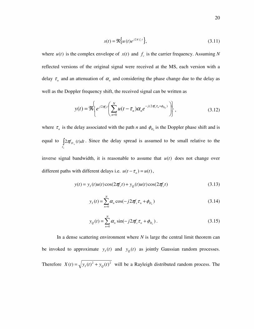
analysis, narrowband fading described by the Clarke’s model [7] is adopted. Let the
transmitted signal be
20
{ }tfj cetutsπ2
)()( ℜ= , (3.11)
where )(tu is the complex envelope of )(tx and cf is the carrier frequency. Assuming N
reflected versions of the original signal were received at the MS, each version with a
delay nτ and an attenuation of nα and considering the phase change due to the delay as
well as the Doppler frequency shift, the received signal can be written as
−ℜ= ∑
=
+−N
n
fj
nn
tfj nDncc etuety0
)2(2)()(
φτππ ατ , (3.12)
where nτ is the delay associated with the path n and nDφ is the Doppler phase shift and is
equal to ∫n
ndttfD
τ
π )(2 . Since the delay spread is assumed to be small relative to the
inverse signal bandwidth, it is reasonable to assume that )(tu does not change over
different paths with different delays i.e. )()( tutu n =−τ ,
)2cos()()()2cos()()()( tftutytftutyty cQcI ππ += (3.13)
∑=
+−=N
n
DncnI nfjty
0
)2cos()( φτπα (3.14)
∑=
+−=N
n
DncnQ nfjty
0
)2sin()( φτπα . (3.15)
In a dense scattering environment where N is large the central limit theorem can
be invoked to approximate )(tyI and )(tyQ as jointly Gaussian random processes.
Therefore 22 )()()( tytytX QI += will be a Rayleigh distributed random process. The

21
Clarke’s model also defines the temporal properties of this process with its auto-
covariance
)2()(2
22 τπτ doXXfJC
ii
= , (3.16)
which is expressed in the discrete time domain as
)2()(2
22 lTfJlC sdoXX ii
π= , (3.17)
where )(xJo is the zeroth order Bessel function of the first kind and df is the maximum
Doppler frequency.
The Rayleigh fading process can be simulated using several techniques. The sum
of sinusoids technique described in [8] was used for the simulations in the following
chapters. A comparison between the auto-covariance of the theoretical and simulated
processes is shown in Figure 10.
0 5 10 15 20 25 30 35 40 45 50-0.6
-0.4
-0.2
0
0.2
0.4
0.6
0.8
1
Time index
Auto
covariance
Theoretical
Simulated
Fig. 10. Auto-Covariance of the Simulated Rayleigh Process Against Theoretical Bessel Auto-Covariance

22
CHAPTER IV
HANDOFF PERFORMANCE – SLOT ERROR PROBABILITY
A. Introduction
This chapter includes an analytical approach to study the performance of the
handoff algorithm in 1xEV-DO REV. A systems through the slot error probability. The
approach is based on a simplified performance model usually used for system
simulations. This simplification is necessary since in REV. A systems the downlink
transfer rates are high (up to 3.072 Mbps) which makes link level simulations employing
symbol level detection and turbo coding computationally intensive. As an alternate
solution slot simulations are used. For every slot period, the signal to interference and
noise ratio (SINR) is determined and then compared to a threshold to decide whether an
error has occurred.
The analytical approach is also verified using SEP simulations over parameters
of practical interest.
B. System Model and the Handoff Algorithm
The MS is assumed to be at equal distance from four base stations as shown in
Figure 11. At any point of time the MS will be connected to one of the four BSs, while

23
the rest are considered to be interferers. Based on the channel model presented in
Chapter III, the power of the signal received from BSi (in decibels) is
))((log10)( 2
10 nXnYP iii += , (4.1)
where Yi(n) represents the combined path loss and shadow fading components and Xi(n)
represents the Rayleigh fading component.
Fig. 11. The Four Cell Model
The MS should be generally connected to the BS that will provide the highest
signal to interference power ratio to achieve best performance. However, to avoid
unnecessary handoffs resulting from the rapid signal changes imposed by the Rayleigh
fading, the received signal to interference ration (SIR) is filtered, allowing for better
tracking of the average signal strength. Furthermore, the algorithm requires the filtered
SIR from BSi to exceed the one from BSj by a specified hysteresis before initiating a

24
handoff from BSj to BSi. The hysteresis will protect the system from rapid continuous
handoffs between the BSs, which is known as the ping-pong effect.
The SIR at the MS when it is being served by BSi is
)()()( nPnPnSiii Σ−= , (4.2)
where )10(log10)(10/)(
10 ∑≠
Σ =N
ij
nP
i
jnP . The filtered SIR is given by
)()()( nhnSnF ii ∗= , (4.3)
where h(n) is the filter’s impulse response and ∗ denotes linear convolution. The handoff
request can then be written as
,)1(
)()(4
)()(3
)()(2
)()(1)(
4
3
2
1
max4
max3
max2
max1
otherwisenR
HnFnF
HnFnF
HnFnF
HnFnFnR
−=
≥−=
≥−=
≥−=
≥−=
(4.4)
where )(max nFi
is )]([max nFjij ≠
and inR =)( is the request at time n to connect to BSi.
C. Slot Error Probability Evaluation
By definition a slot error is assumed to occur if the received SIR drops below a
specified threshold (T). This means that a slot error occurs if BSi is serving the MS and
Si(n) < T.
∑ ∫∞−
==i
T
ii dSinCnSfSEP ))(),(( , (4.5)
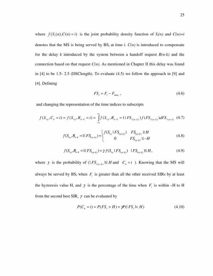
25
where ))(),(( inCnSf i = is the joint probability density function of Si(n) and C(n)=i
denotes that the MS is being served by BSi at time i. C(n) is introduced to compensate
for the delay k introduced by the system between a handoff request R(n-k) and the
connection based on that request C(n). As mentioned in Chapter II this delay was found
in [4] to be 1.5- 2.5 (DSClength). To evaluate (4.5) we follow the approach in [9] and
[4]. Defining
iFFFS ii max−= , (4.6)
and changing the representation of the time indices to subscripts
∫∞
∞−
−−−−− =====)()()(
)()|1,(),(),(kniknikniknniknninni dFSFSfFSRSfiRSfiCSf (4.7)
−≤
≥==
−
−−
−− HFS
HFSFSSfFSRSf
kni
kniknini
kniknni
)(
)()(
)( 0
)|()|1,( (4.8)
HFSFSSfFSRSfknikninikniknni ≤==
−−−− ||)|()|1,()()()(
γ , (4.9)
where γ is the probability of ( HFSkni ≤
−||
)(and iCn = ). Knowing that the MS will
always be served by BSi when iF is greater than all the other received SIRs by at least
the hysteresis value H, and γ is the percentage of the time when iF is within –H to H
from the second best SIR, γ can be evaluated by
)|(|)()( HFSPHFSPiCP iin <+>== γ (4.10)

26
,
)(
)()(
)()()(
∫
∫
∫∫
−
∞
−
∞
−=
=
+==
H
H
ii
H
iin
H
H
ii
H
iin
dFSFSf
dFSFSfiCP
dFSFSfdFSFSfiCP
γ
γ
(4.11)
Moreover since the MS is at equal distance from all BSs and since all Pi’s are identically
distributed, )( iCP n = is equal to 0.25.
The joint distribution of niS and iCn = is
∫∫−
−−
∞
−−+==
H
H
kniknini
H
kniknininni dFSFSSfdFSFSSfiCSf)()()()(
),(),(),( γ . (4.12)
Therefore the slot error probability is given by
∫ ∫∫ ∫∞− −
−−
∞−
∞
−−+=
T H
H
ikniknii
T
H
ikniknii dSdFSFSnSfdSdFSFSnSfSEP ))),(()),(((4)()()()(
γ . (4.13)
To evaluate (4.13) some approximations are made to keep the analysis tractable.
1. Received Power Statistics
The received power at the MS from any of the serving BSs is a product of a
Rayleigh process and a lognormal process. The distribution of the received power is
therefore a composite Rayleigh-lognormal distribution. This distribution is
mathematically intractable, however some alternative distributions can be used to
efficiently approximate it. Over certain ranges of lognormal standard deviation (iYσ >6

27
dB) it is generally acceptable to use a lognormal distribution to approximate the
composite distribution. Since typical shadow standard deviation values range from 5 to
12 dB (with 8.9 dB suggested by the 3rd generation partnership project 2 (3GPP2) in
[6]) we can assume the distribution of received power Pi to be lognormal. The mean and
standard deviation of the new lognormal were found in [10] by calculating the mean and
standard deviation of the Susuki distribution which models the probability density
function of the composite distribution.
∫∞
−
−−
=0
2
2
/
2
)/ln/(lnexp
2
11)( η
σ
λµλη
ησπληη
dePfYi
Y
Y
P
lii
i
li , (4.14)
where 10/)10ln(=λ and 10/
10 iP
liP = .
lililii dPPfPPE )()(log10][0
10∫∞
= , (4.15)
lililii dPPfPPE )())(log10(][ 2
0
10
2
∫∞
= . (4.16)
Equations (4.15) and (4.16) were solved in [10] to find the new mean and standard
deviation as follows
,5.2 dBYiPi −= µµ (4.17)
2257.5+=
iYPi σσ , (4.18)
The correlation between the different powers received from different base stations can
be found by using equations from [11]

28
ji
ljli
ji
PP
PP
ljli
PP
MM
PP
σσλρ
2
)],cov[
1ln( +
= (4.19)
)2
exp(2
2
iilili YYYP MMM σλ
λ +== , (4.20)
where 10/)10ln(=λ ,10/
10 iP
liP = ,iYM and
iYσ are the mean and standard deviation of iY ,
respectively, liPM and
liPσ are the mean and standard deviation of liP , respectively.
ljliljliljliljli YYjiYYYYYYljli MMXXEMMPP −+= ][)(],cov[22
σσρ (4.21)
)1))(exp(1)(exp(
1)exp(
2222
2
−−
−=
ji
jiji
ljli
YY
YYYY
YYσλσλ
σσρλρ (4.22)
)1))(exp(2exp(22222
−+=iiili YYYY M σλσλλσ , (4.23)
where 10/
10 iY
liY = , liYM is the mean of liY and
liYσ is the standard deviation of liY .
2. Signal to Interference Ratio Statistics
The signal to interference ratio (SIR) is defined in (4.2) as )()()( nPnPnSiii Σ−= .
Therefore, to find )(nSi ’s distribution we need to find the distribution of )(nPiΣ , where
)(nPiΣ is the linear summation of a group of lognormals. This problem of finding the
distribution of the sum of a group of lognormals has been extensively studied due to its
importance in the analysis of interference in wireless and especially cellular systems. A
simple yet a good solution assumes the distribution of the sum of the lognormals to be

29
also lognormal. Based on this assumption the Schwartz and Yeh’s method [12] evaluates
the mean and standard deviation of the new lognormal by matching them to those of the
sum in the dB domain. The method starts by finding a numerical solution for the mean
and standard deviation for the sum of only two lognormals. Then based on the
assumption that the new distribution is also lognormal the procedure is repeated to find
the new mean and standard deviation as follows,
ilii PPQ λ== ln (4.24)
iiii PQPQ λσσλµµ == , , (4.25)
where Qi is introduced to simplify the analysis.
)ln(∑≠
Σ =ij
Q
i
jeQ (4.26)
)ln(,kj QQ
kj eeQ += (4.27)
)][ln(][,,
kj
kj
Qkj eeEQE +== µ (4.28)
)]([ln][ 2222
, ,,
kj
kjkj
QQkj eeEQE +=+= σµ (4.29)
Rearranging equation (4.28)
,)]1[ln(
)]1[ln()][ln(,
j
k
j
j
k
j
kj
Q
Q
Q
Q
Q
e
eE
e
eEeE
++=
++=
µ
µ (4.30)
where )]1[ln(j
k
Q
Q
e
eE + is calculated numerically keeping in mind that
j
k
Q
Q
e
e is also
lognormal. Using the same approach 2
,kjQσ is evaluated.

30
Applying this approach recursively and taking into consideration the correlation
between different lognormals, [13] shows how to find the mean and standard deviation.
Starting with
11 QZ = , (4.31)
and defining
jiji
kk
PPQQ
QZ
ki eeZQZ ρρ =+== −
Σ ),ln(, 1 , (4.32)
we have
),(11 kkkk wwZZ G σµµµ +=−
(4.33)
),()(
2),(),( 32
))((
2
2
1122 111
kk
k
kkkkk
kkkkk
k www
ZZQQZ
wwwwZZ GGG σµσ
σσσρσµσµσσ −−−
−
−−+−= (4.34)
),(11
11
2211
1
21 32
))(())(())(2(
))(( −−
−−
−−−−
−
−−
−+=
−
kk
kk
kkkkk
k
k
kkk ww
wZ
ZQkZQQQ
z
QZk
ZQZ G σµσσ
σρσρ
σ
ρσρ , (4.35)
where kwµ and
kwσ are the mean and standard deviation of
1−−= kkk ZQw , (4.36)
and are equal to
1−−=
kk ZQkw µµµ (4.37)
22
1−+=
kkk ZQw σσσ . (4.38)
G1, G2 and G3 are evaluated numerically and are given by
)}1{ln(),(1k
kk
w
ww eEG +=σµ (4.39)
)}1({ln),( 2
2k
kk
w
ww eEG +=σµ (4.40)

31
)}1ln(){(),(3k
kkk
w
wkww ewEG +−= µσµ . (4.41)
Finally
λσσλµµ /,/NiNi ZPZP ==
ΣΣ. (4.42)
Since both )(nPi and )(nPiΣ are assumed to be normally distributed, the outcome of the
subtraction of )(nPiΣ from )(nPi is normally distributed as well with mean and standard
deviation given repectively by
iiiiiiiii PPiPPPPSPYS MMM∑∑∑∑
−+=−= σσρσσσ 2,222
. (4.43)
The correlation between different SIRs can be found using an approach similar to that
presented in [14]. In general, the correlation between different sums of lognormals can
be calculated as follows
)]10.....1010()10.....1010[(]1010[
)10.....1010(log10
)10.....1010(log10
10/10/10/10/10/10/10/10/
10/10/10/
10
10/10/10/
10
2121
21
21
MN
M
N
PPPPPPBA
PPP
PPP
EE
B
A
++=
+=
+=
∑∑∑∑= =
++++
= =
+==
N
i
M
j
MMN
i
M
j
PP jPiPjPiPjPiPPjiP
ji eE1 1
)2(2
1
1 1
10/)(222
]10[σσρσσλλλ
. (4.44)
Then again from [11]
BA
BA
BA
AB
MM
E
σσλρ
2
10/10/
)]1010[
1ln( +
= . (4.45)
An extension to Wilkinson’s approach is used to find the auto and cross-
covariance functions between different SIRs. The approach is based on matching the

32
auto-covariance function of the new process to that of the summation of the lognormals
in the linear domain and then transferring it back to the dB domain.
The cross-covariance between two correlated shadow fading processes was found
in [15]
)()( lClCiijiji YYYYYY ρ= , (4.46)
and the auto-covariance of the Rayleigh fading process Xi is given by
1)2()]()([)( 2222 +=+= lTfJolnXnXElR sdiiX i
π . (4.47)
Therefore the auto-correlation function between two shadow fading processes in the
linear domain is [16]
))()(2
1)(2exp(]1010[)(
22210/)(10/)(lCMMElR
jijijiljli YYYYYY
lnYjnYi
YY ++++== + σσλλ , (4.48)
and the auto-correlation function between the power received from BSi and the power
received from BSj in the linear domain is
)),()(2
1)(2exp()(
]1010[)()(
222
10/)(10/)(
22
22
lCMMlR
ElRlR
jijijiji
ji
jiljli
YYYYYYXX
lnPnP
XXPP
++++=
=+
σσλλ (4.49)
where liili YXP2
= . Again in general if
)10.....1010(log10
)10.....1010(log10
10/10/10/
10
10/10/10/
10
21
21
M
N
PPP
PPP
B
A
+=
+=
then

33
∑∑= =
++++
+++
+
=
++=
N
i
M
j
lCMM
XX
lnPlnPlnPnPnPnP
lnBnA
jYiYjYiYjYiY
ji
MN
elR
E
E
1 1
)()(2
1)(
10/)(10/)(10/)(10/)(10/)(10/)(
10/)(10/)(
222
22
2121
)(
)]10.....1010)(10.....1010[(
]1010[
σσλλ
(4.50)
222210/)(10/)(/))(
2
1])1010[(ln()( λσσλλ BABA
lnBnA
AB MMElC +−−= + . (4.51)
The auto-covariance function between any two SIRs is
)]()([)]()([)]()([)]()([
))]()(())()([()(
lnPnPElnPnPElnPnPElnPnPE
lnPlnPnPnPElC
jijijiji
jjiiSS ji
+++−+−+=
+−+−=
∑∑∑∑
∑∑
)()()()( lClClClCjijij PPPPPiPPiPj ∑∑∑∑
+−−= , (4.52)
where the covariance functions in (4.52) are evaluated using (4.51).
3. Filtered SIRs Statistics
The filter used to eliminate the fast Rayleigh fading variations is typically a first
order IIR low pass filter [9]. The impulse response of the filter was chosen in [4] to be
n
iiriir TTnh )/11)(/1()( −= . (4.53)
Since the filter is linear the filtered SIRs will also be normally distributed with mean
ii SiF FE µµ == ][ . (4.54)
The auto and cross-covariance functions between filtered SIRs and filtered and
unfiltered SIR’s are
)()()()]()([)()()]()([)( lClClhlSlSlhlSlSlhlCjijiji FSSSjijiSF =∗=−∗∗=−∗∗= (4.55)
),()()()]()([)]()([)( lClhlhlSlhlSlhlCjiji SSjiFF ∗−∗=−∗−∗∗= (4.56)

34
where ||)/11)(/1()()( l
iiriir TTlhlh −=−∗ [17]. Standard deviations of the filtered SIRs
along with different correlation coefficients can be found using the filtered auto and
cross-covariance functions
)0(iii FFF C=σ (4.57)
)/()0(jijiji FFFFFF C σσρ = (4.58)
)/()()( jijiknji FSSFFS kC σσρ −=
−. (4.59)
4. The Maximum of a Group of Filtered SIRs
As mentioned before when the MS is being served by BSi, a handoff operation
will only be initiated if the received SIR from any other BS ( jF ) is greater than the
current filtered SIR iF by the heteresis value H. In other words, if the maximum of the
three filtered SIRs (i
Fmax ) exceeds the current filtered SIR by H, then the MS initiates a
handoff request. Therefore finding the distribution of the maximum of the three
remaining filtered SIRs is essential for the analysis of the handoff performance. Since in
the previous sections the filtered SIRs were approximated by normal distributions, the
Clark’s approach can be used to find the distribution of their maximum. The approach
starts by matching the moments of a new normal distribution to that of the maximum of
only two. The same procedure is then repeated using a pair at a time. Clearly the
approximation is more accurate for the case of a small number of random processes
(three in this case), since the assumption of the maximum being normally distributed

35
becomes less accurate as the number of random processes increases. The approach starts
by defining
)2
exp(2
1)(
2x
x −=π
φ (4.60)
∫∞−
=Φy
dxxy )()( φ (4.61)
5.22)2(
jljljl FFFFFFa σσρσσ −+= (4.62)
a
jl FF µµα
−= . (4.63)
Then for ),max(,max jljl FFF = the mean and the variance are
)()()(,max
αφαµαµµ aFjFlF jl+−Φ+Φ= (4.64)
222222
,max,max)()()()()()(
jljl FFjFlFjFlFjFlF a µαφµµαµσαµσσ −++−Φ++Φ+= . (4.65)
The maximum of three random processes can be found by evaluating ),max( ,max mjl FF .
This can be done simply by redefining the variables in equations (4.60) (4.61) (4.62) and
(4.63) then calculating the mean and variance from (4.64) and (4.65), where
jl
jmjmml
mjl
F
FFFFFF
FF
,max
,max
)()(
σ
ασρασρρ
−Φ+Φ= . (4.66)
Using (4.66) we can also find the correlation coefficient between the maximum of the
filtered SIRs (i
Fmax ) and the fourth filtered SIR ( iF ) as well as the unfiltered SIR ( iS )
i
mmklijl
ii
F
FFiFFFF
FF
max
,max,max
max
)()(
σ
ασρασρρ
−Φ+Φ= (4.67)

36
jl
jikniikn
iknjl
F
FSFjFSFl
SF
,max
)()(
)(,max
)()(
σ
ασρασρρ
−Φ+Φ= −−
− (4.68)
i
miknmkliknjl
ikni
F
FSFFSF
SF
max
)(,max)(,max
)(max
)()(
σ
ασρασρρ
−Φ+Φ=
−−
−, (4.69)
where the bracketed subscripts indicate time, and all the unindexed variables are
assumed to be at time n. For i
FFFS ii max−= the mean and standard deviation are
iiiiiiiiii FFFFFFFSFFFS MMM
maxmaxmax
max2, 222 σσρσσσ −+=−= , (4.70)
and the correlation coefficient between iFS and iS is
)/()(max)(max)( iiiiikniiiiknii SFSSFSFSFSFiSFS σσσσρσσρρ
−−−= (4.71)
To verify the validity of our approximations, Figure 12 shows a comparison between the
approximated cumulative distribution function (CDF) of FSi and a simulated one.
-60 -40 -20 0 20 40 600
0.1
0.2
0.3
0.4
0.5
0.6
0.7
0.8
0.9
1
FSi (dB)
CD
F
Actual
Approximated
Fig. 12. A Comparison Between the Approximated CDF and a Simulated CDF of FSi

37
Using the previous results, the SEP can now be evaluated using (4.13).
D. SEP Numerical and Simulation Results
To confirm the accuracy of the proceeding analytical analysis over parameters of
practical interest computer simulations were carried out according to the system model
and handoff algorithm described in Chapter II. The communication channel was
simulated as described in Chapter III. While analytical based results were obtained using
(4.13). The system parameters are listed in Table II.
Table II
Simulation System Parameters
Carrier frequency cf 1.9 GHz
Shadow fading standard deviation iYσ 8.9 dB
Correlation coefficient between shadow fading components jiYYρ 0.5
Decorrelation distance for shadow fading corrd 20 m
First path loss constant 1K 20 dB
Second path loss constant 2K 50 dB
Sampling period sT 1.667 ms

38
A comparison between numerical and simulated results using the cumulative
distribution function (CDF) of the SIR received at the MS is shown in Figure 13. This
CDF was obtained by varying the value of T in (4.13). The figure shows that the
numerical values of the SEP match closely the simulated ones with increasing accuracy
for higher MS speed. Hence, in subsequent figures only the numerical results are shown
for the SEP.
-20 -15 -10 -5 0 5 10 15 2010
-3
10-2
10-1
100
SIR (dB)
CD
F
Numerical v=10 m/s
Simulated v=10 m/s
Numerical v=30 m/s
Simulated v=30 m/s
Numerical v=70 m/s
Simulated v=70 m/s
Fig. 13. Numerical and Simulated Results Comparison
The combined effects of the MS speed, the DSC length and the filter constant are
captured is Figure 14.

39
1 16 32 640
0.02
0.04v=3 m/s
1 16 32 640
0.05v=10 m/s
SE
P %
1 16 32 640
0.1
0.2v=80 m/s
DSC length
Tiir=16
Tiir=32
Tiir=64
Tiir=128
Fig. 14. Effects of DSC Length and TIIR on SEP at Different MS Speeds
As shown in Figure 14, at low speeds when the system delay is minimal (DSC
length is equal to 1 slot) a lower TIIR means better tracking of the relatively slowly
varying Rayleigh fading and hence lower SEP. As TIIR increases the ability of tracking
the Rayleigh fading variations decreases causing the SEP to increase. But as the system
introduced delay increases this close tracking of the Rayleigh fading variations becomes
a disadvantage, since by the time a requested handoff is executed the SIR will have
moved to a new state. Therefore, more filtering is advantageous since it filters out fast
SIR changes with which the system is unable to catch up.

40
At medium speeds the relatively fast variations of the Rayleigh fading are filtered
out. Moreover, the shadow fading is slowly changing and can be generally tracked using
any of the suggested TIIR values. Therefore, the increase of SEP with increasing TIIR is
caused by the increase of filtering delays. This increase is more noticeable for small
DSC lengths since at large DSC lengths the system introduced delay is greater than that
of the filtering and contributes more to the increase of SEP.
At higher speeds Rayleigh fading variations are still assumed to be filtered out.
However shadowing variations will increase, and since smaller filter constants allow for
better tracking of these variations, SEP is expected to increase when TIIR is increased at
different DSC lengths.

41
CHAPTER V
HANDOFF PERFORMANCE - PACKET ERROR AND HANDOFF RATES
A. Introduction
The effects of different system parameters on the handoff performance were
studied through SEP in the previous chapter. However, in packet switched systems the
packet error rate (PER) is a more important measure in determining system performance.
Therefore this chapter discusses the effects of the same system parameters on PER, in
order to understand the insight gained about PER from SEP. Unlike SEP, PER results
are obtained through simulations only. This is due to the analytical complexity imposed
by packet transmission techniques employed in the Rev. A systems such as the H-ARQ.
Another important measure that must be kept in mind when analyzing handoff
performance is the handoff rate, since frequent handoffs will increase the load on the
network and therefore will lead for service degradation. Again only simulation results
were used for the analysis of the handoff rate. Finally tradeoffs between different
performance measures are presented at the end of this chapter.
B. Packet Error Rate Simulation Technique
As mentioned in the previous chapter running link level simulations for EV-DO
systems is a computationally intensive operation. However, the simulation flow for PER
is affected by decisions made of whether the data in a packet was successfully decoded

42
or not. Therefore, in able to run slot level simulations, a technique is needed by which
we can estimate the probability of decoding a packet correctly at the MS based on the
SIRs associated with the pilots of the received sub-packets. An interesting technique is
presented in [18], where the probability of decoding a packet correctly is calculated
based on results obtained previously by running full simulations.
In general PER versus received SIR plots are obtained from link level
simulations. These graphs can be then used in slot level simulations, where every time a
slot is received the PER value corresponding to the received SIR of that slot is looked up
from the graphs. Then based on this PER, we pseudo randomly determine if the packet
was correctly decoded or not.
Fig. 15. PER vs. Received SIR Approximated Model
In practice, SEP versus received SIR graphs are approximated by the graph in
Figure 15 , where rγ is the received SIR, 01.0γ is the SIR required to achieve 1% PER,

43
∆γ is the required increase in SIR to decrease the PER by a factor of ten and Mγ is the
implementation margin which accounts for various losses, and is assumed to be equal to
2 dB [19].
From Figure 15 PER is equal to
−+>
= ∆
+−−− ∆∆
elsePER Mr
r
Mr
,1
2,10)( 01.0
)/)2(( 01.0 γγγγγ
γγλγγ
(5.1)
Table III carries values for 01.0γ and ∆γ obtained in [3]. This table only shows
values for the data rate of 38.4 kbps with the packet length of 16 slots. Using this table
the simulation can be run as explained below and in the flow chart in Figure 16:
• Upon the reception of a new sub-packet the linear average of all the
received sub-packets’ SIRs is found.
• Based on the average SIR and the number of the received sub-packets
Table III is used to look up 01.0γ and ∆γ values.
• PER is calculated using (5.1).
• Based on the calculated PER we pseudo randomly determine whether the
packet was successfully decoded or not.
• The above procedure is repeated until the packet is successfully decoded
or until all the sub-packets are sent.

44
Fig. 16. PER Simulation Flow Chart
Table III
Simulation Parameters for 38.4 kbps Data Rate
Sub-packet Number
Effective Data Rate
γγγγ0.01r(dB) γγγγ∆∆∆∆(dB)
1 614.40 6.7 0.28
2 307.20 -2.9 0.28
3 204.80 -5.3 0.30
4 153.60 -6.9 0.30
5 122.88 -8 0.30
6 102.40 -8.9 0.30
7 87.77 -9.7 0.28
8 76.80 -10.3 0.29
9 68.27 -10.8 0.29
10 61.44 -11.3 0.29
11 55.85 -11.8 0.29
12 51.20 -12.2 0..30
13 47.26 -12.5 0.30
14 43.89 -12.9 0.31
15 40.96 -13.2 0.30
16 38.40 -13.5 0.45

45
Figure 17 shows the PER for 38.4 kbps data rate. The simulations were carried
out as explained before. The effects of different parameters on PER are very similar to
those on SEP. However since PER benefits from H-ARQ, some interesting points can be
discussed.
At low speeds, it is clear that the most significant gain due to H-ARQ happens at
large DSC lengths with large filter constants. This is due to the fact that at low speeds
when the Rayleigh fading is still tractable by small filter constants, large filter constants
are able to average fast changes in the SIR. This averaging will increase operation times
at which the received SIR is good, and therefore increase the probability for most sub-
packets to be transmitted at these good channel conditions. Although some sub-packets
might be transmitted at the instances with bad channel conditions caused by the fast
variations, their effect will be compensated for by the good sub-packets. On the other
hand, at medium speeds it is shown that least achieved H-ARQ gain is at large DSC
lengths with large filter constants. This is due to the fact that at these speeds where the
Rayleigh fading is generally filtered out by all the suggested values of filter constants,
larger filter constants introduce more filtering delays. Adding these delays to the large
DSC channel delay, the MS might stay in bad channel conditions for some time before it
is handed over to another BS, which will clearly increase the chance for the transmitted
sub-packets to fall into bad channel conditions. Another observation that is worth noting
is that the H-ARQ gain does not appear to be significant at high speeds. This is due to
the fast variations of the communication channel at such speeds, which reduces the
overall efficiency of the handoff algorithm in all cases.

46
1 16 32 640
0.02
0.04v=3 m/s
1 16 32 640
0.05
0.1
PE
R%
v=15 m/s
Tiir=16
Tiir=32
Tiir=64
Tiir=128
1 16 32 640
1
2
DSC length
v=80 m/s
Fig. 17. Effects of DSC Length and TIIR on PER at Different MS Speeds
C. PER with Maximal Ratio Combining
To increase data throughput receiver diversity techniques are used in EV-DO
systems. In receiver diversity, multiple antennas are used at the receiver. The separation
between antennas must be sufficient to assume independent fading on different paths
from the transmitter to different antennas. This independence lowers the probability of
experiencing simultaneous deep fades.
At the receiver different paths can be combined in different ways. Most
techniques combine the paths linearly, where the outcome is a weighted sum of the
different paths. The technique that achieves maximum output SINR at the receiver is

47
called the maximal ratio combining (MRC). In this technique every path is multiplied by
a value proportional to the SINR experienced on that channel before adding it up to other
paths.
Figures 18 and 19 show PER values simulated at 38.4 and 153 kbps with MRC.
The SIRs received at the two antennas are assumed to be independent and identically
distributed. The distribution for each antenna follows the channel model in Chapter IV.
The figures show clear PER improvement achieved by MRC. Figure 19 also shows that
applications that require higher data rates can be reliably served by the 1xEV-DO Rev. A
systems employing seamless server selection with H-ARQ and receive diversity.
1 16 32 640
0.01
0.02v=3 m/s
1 16 32 640
0.005
0.01
PE
R%
v=15 m/s
Tiir=16
Tiir=32
Tiir=64
Tiir=128
1 16 32 640
0.2
0.4
DSC length
v=80 m/s
Fig. 18. Effects of DSC Length and TIIR on PER at 38.4 kbps with MRC

48
1 16 32 640
2
4v=3 m/s
1 16 32 640
2
4
PE
R%
v=15 m/s
Tiir=16
Tiir=32
Tiir=64
Tiir=128
1 16 32 640
5
10
DSC length
v=80 m/s
Fig. 19. Effects of DSC Length and TIIR on PER at 153 kbps with MRC
D. Handoff Rate
Another important measure of the handoff performance is the handoff rate.
Although it is desirable to change the serving BS whenever the MS can achieve better
PER, frequent handoffs require more system resources and increase the chance of
service interruption. Figure 20 shows handoff rates for different system parameters. The
figure shows that the number of handoffs decreases with an increasing TIIR since less
fluctuation in the filtered SIRs will result in longer operating times for each BS before a
handoff is initiated. Moreover it also shown that the number of handoffs slightly
decreases with increasing DSC length, since recurring delays in the handoff execution
will limit the number of handoffs occurring in a period of time.

49
1 16 32 640
10
20v=3 m/s
Tiir=16
Tiir=32
Tiir=64
Tiir=128
1 16 32 640
5
10
Handoff
rate
v=15 m/s
1 16 32 640
5
10
DSC length
v=80 m/s
Fig. 20. Effects of DSC Length and TIIR on Handoff Rate at Different MS Speeds
Although one would expect a direct tradeoff between the handoff rate and the
PER, results obtained in this chapter prove that this is not always the case. The fact that
there is an introduced system delay makes large filter constants (in some cases) more
desirable is terms of PER, in addition to the reduced handoff rate these constants can
achieve. As a result, we observe that for practical DSC lengths, moderately large filter
constants (TIIR=64 in our case) will generally achieve better system performance for low
and medium MS speeds. Moreover, their performance at high MS speeds is not
significantly worse than that of smaller filter constants. Therefore, keeping in mind that
handoff rates for such constants are usually low, it is generally desirable to pick large
filter constants in practical systems.

50
CHAPTER VI
CONCLUSIONS AND FUTURE WORK
The performance of the handoff technique used in 1xEV-DO Rev. A systems was
studied. Slot error probability (SEP) in addition to packet error rate (PER) and handoff
rate were used as performance measures. An analytical approach was developed to
evaluate the SEP, while PER and handoff rates were obtained using slot level
simulations. Unlike previous work we adopted a multiple base station system model and
accounted for correlation between shadowing components in the channel model.
Moreover the effects of system parameters such as the handoff filter, DSC length and
mobile station’s speed on system performance measures were studied.
It was found that although absolute values of SEP and PER cannot be directly
compared due the H-ARQ gain in PER, the insight gained from both of them about the
system parameters effects is generally the same. It was also found that the used handoff
technique in 1xEV-DO Rev. A systems can achieve acceptable performance when
employing H-ARQ and receive diversity on the downlink. Finally it was found that in
general moderately large filter constants are more desirable for practical DSC lengths.
Moreover the results found can be used to specify system parameters based on different
PER requirements and other system conditions.
The system model developed in this thesis can be further improved by including
a flexible number of base stations serving a mobile station located at different distances
from each base station. Packet simulations can also be enhanced to include actual data

51
rate requests based on the channel conditions rather than using a fixed data rate on the
downlink. Finally, the analytical approach can be extended to obtain numerical results
for the PER and handoff rate to replace the simulated ones.

52
REFERENCES
[1] 3rd Generation Partnership Project 2 (3GPP2), “cdma2000 high rate packet data air
interface specification,” Technical Report C.S20024-A v1.0, Mar. 2004.
[2] N. Bhushan, C. Lott, P. Black, R. Attar, Y. Jou, M. Fan et al., “cdma2000 1xEV-
DO revision A: A physical layer and MAC layer overview,” IEEE Commun. Mag.,
vol. 44, no. 2, pp. 75- 87, Feb. 2006.
[3] M. Yavuz, D. Paranchych, G. Wu, G. Li, and W. Krzymień, “Performance
improvement of the HDR system due to hybrid ARQ,” in Proc. IEEE Vehic. Tech.
Conf., Atlantic City, NJ, Oct. 2001, vol. 4, pp. 2192-2196.
[4] C. Patel, M. Yavuz, and Y. Tokgoz, “Handoff performance analysis for 1xEV-DO
Rev. A systems,” in Proc. IEEE Int. Conf. Commun., Istanbul, Turkey, Jun. 2006,
vol. 11, pp. 4924-4929.
[5] M. Gudmundson, “Correlation model for shadow fading in mobile radio systems”,
IEE Elec. Lett., vol. 27, no. 23, Nov. 1991.
[6] 3GPP2 TSG-C WG3, “1xEV-DO evaluation methodology,” TSG-C Contribution
C30-20031002-004, Oct. 2004.
[7] R.H. Clarke, “A statistical theory of mobile-radio reception,” Bell Syst. Tech. J.,
vol. 47, pp. 957-1000, Jul.-Aug. 1968.
[8] M. Patzold, U. Killat, F. Laue, and Y. Li, “On the statistical properties of
deterministic simulation models for mobile fading channels,” IEEE Trans. Veh.
Technol., vol. 47, pp. 254-269, no. 1, Feb. 1998

53
[9] S. Das, W. M. MacDonald, and H. Viswanathan, “Sensitivity analysis of handoff
algorithms on CDMA forward link,” IEEE Trans. Veh. Technol., vol. 54, no. 1, pp.
272-285, Jan. 2005.
[10] M. D. Turkmani, “Probability of error for M-branch macroscopic selection
diversity,” in Proc. Inst. Elect. Eng-I Commun., Speech and Visions, vol. 139, Feb.
1992, pp. 71-78.
[11] A.M. Law, and W.D. Kelton, Simulation Modeling and Analysis, 4th Edition,
Boston, MA: Mc.Graw Hill, 2007.
[12] S. Schwratz and Y. S. Yeh "On the distribution function and moments of power
sums with lognormal components," Bell Syst. Tech. J., vol. 61, pp.1441-1462, Sep.
1982.
[13] A. Abu-Dayya and N. C. Beaulieu, “Outage probabilities in the presence of
correlated lognormal interferers,” IEEE Trans. Veh. Technol., vol. 43, pp. 164–
173, Feb. 1994.
[14] A. Ligeti, “Outage probability in the presence of correlated lognormal useful and
interfering components,” IEEE Commun. Lett., vol. 4, pp. 15-17, Jan 2000.
[15] F. Graziosi and F. Santucci, “A general correlation model for shadow fading in
mobile radio systems,” IEEE Commun. Lett., vol. 3, pp. 102–104, Mar. 2002.
[16] C. Fischione, F. Graziosi, and F. Santucci, “Approximation of a sum of onoff
lognormal processes with wireless applications,” in Proc. of IEEE Int. Conf.
Commun., Paris, France, Jun. 2004, vol. 1, pp. 306-310.

54
[17] J.G. Proakis and D.G. Manolakis, Digital Signal Processing: Principles,
Algorithms, and Applications, 3rd ed. Englewood Cliffs, NJ: Prentice-Hall, 1996.
[18] D.W. Paranchych and M. Yavuz "A method for outer loop rate control in high data
rate wireless networks," in Proc. IEEE Veh. Technol. Conf., Vancouver, Canada,
Sep. 2002, vol. 3, pp. 1701-1705.
[19] P. Bender, P. Black, M. Grob, R. Padovani, N. Sindhushayana, and A. Viterbi,
“CDMA/HDR: A bandwidth efficient high-speed wireless data service for nomadic
users,” IEEE Commun. Mag., vol. 39, no. 7, pp. 70-77, Jul. 2000.

55
VITA
Name: Maher Al-Shoukairi
Address: 214 Zachry Engineering Center, College Station, Texas 77843
Email Address: [email protected]
Education: B.S., Electrical Engineering, University of Jordan, Jordan, 2005
M.S., Electrical Engineering, Texas A&M University, 2008