1

Performance Measures for GPS Anti-Jam Antenna Arrays

Dr. Ronald L. Fante The MITRE Corporation

202 Burlington Road Bedford, MA 01730

Abstract

We have derived analytical expressions for the signal-to-interference ratio, jammer-to-noise ratio, carrier phase error and code tracking error at the crosscorrelator output of the code-tracking loop in a GPS receiver that uses adaptive space-time processing to cancel interference. In the limit when the adaptive processor is absent, and all channels are perfectly matched, these results reduce to the performance measures derived previously. Acknowledgments

The author is grateful to P. J. Costa, D. Moulin, K. F. McDonald, and N. R. Shnidman for valuable technical discussions.

1. Introduction

Because GPS (Global Positioning System) operation is critical for many applications,

it is necessary for receivers to operate even in hostile interference environments. That is, in order to deny GPS operation, an adversary may use multiple jammers that radiate interference either over the entire GPS operating bandwidth or selected portions thereof. The GPS user must counter this threat. This can be done by using an antenna array that employs space-time-adaptive [1-14] processing; this allows the GPS receiver to place broadband antenna-pattern nulls in the directions of any interferers, while simultaneously preserving the gain in the directions of the desired GPS satellites. In the past, a number of measures have been used to assess adaptive antenna performance, but these measures evaluate only the performance of the adaptive antenna and ignore end-to-end system performance. This deficiency is remedied here.

2

2. Background A GPS receiver processes signals from most (if not all) of the GPS satellites in view.

For each satellite signal, the satellite-to-receiver delay (for precision systems, the phase is also estimated) is estimated, and the delays from multiple satellites are then combined to estimate the position of the GPS receiver. In the absence of interference, this process is well-understood [15-18]. However, when an adaptive processor is inserted into the processing chain, the received signals from each GPS satellite may be attenuated, distorted, and shifted in time, yielding degraded performance. Our goal is to quantify this degradation.

Let us refer to Figure 1, where we show the code-tracking portion of a GPS receiver for

the case when an adaptive space-time processor is inserted to cancel interference. We show radiation arriving from an arbitrary direction (θ,φ) in a spherical coordinate system. This incoming radiation is received by each of the N elements in the antenna array, downconverted to baseband and then bandlimited using a digital filter with transfer function HB(f), where f denotes the baseband frequency. In the GPS Anti-Jam system block diagram, we also include the transfer function Hn(f , θ, φ) for each antenna and its associated analog* hardware. The function Hn also includes any uncorrected mismatch from channel-to-channel. The voltages v1 to vN at the output of the bandlimiting filters are then fed into the adaptive processor, which is shown in expanded form in Figure 2. The output of the adaptive filter, consisting of desired GPS signals, residual jammer interference and noise is then crosscorrelated with a stored, delayed replica of the signal s(t) that was transmitted by the GPS satellite. In Figure 1, we show only the signal from one GPS satellite, but, of course, there are signals present from every GPS satellite in view. Likewise, we show only the crosscorrelator for one signal, but there are actually multiple crosscorrelators operating in parallel, each using appropriate stored replicas for other GPS satellites. For each satellite, the tracking loop adjusts the estimated delay τ̂ so as to match the true delay for that satellite. We do not show the phase-locked loop that corrects for phase, but rather assume the carrier phase of the replica has been matched to the carrier phase of the received signal. * In practice, one tries to equalize the analog portion of each channel across the operating bandwidth so as to make Hn the same for all channels, but this cannot be achieved perfectly because the antenna itself has a response that depends on (θ, φ).

3

We first wish to calculate the transfer function H(f, θ, φ) for the dashed block in Figure 1. Suppose a signal incident from the direction (θ, φ) produces a voltage

( ) ( )[ ]cRtf2iexpcRts non −π−− , on antenna n, where Rn(θ, φ) = φθcossinxn θ+φθ+ coszsinsiny nn , c = the speed of light, fo = the carrier frequency, and ( )nnn z,y,x

is the location of antenna n in a Cartesian coordinate system with origin at antenna 1 (which we denote the reference antenna). After downconversion, the signal at antenna n is

( ) [ ]cRf2iexpcRts non π− , which has a Fourier transform ( )[ ]cRff2iexp)f(S no +π , where f is the baseband frequency. Therefore, the Fourier transform Vn(f) of the voltage vn(t) shown in Figure 1 is ( )[ ]cRff2iexp)f(S),,f(H)f(H nomB +πφθ . If we use this as the input to channel n of the adaptive filter, it is readily seen that the overall transfer function of the block shown dashed in Figure 1 is

( ) ⎥⎦⎤

⎢⎣⎡ −π+φθ+πφθ=φθ ∑∑

==fT)QQq(2i

c),(Rff2iexpw),,f(H)f(H),,f(H n

o

Q

1qnq

N

1nnB , (1)

where mutual coupling* has been ignored, N is the number of antennas in the array, Q is the number of time taps per antenna, T is the intersample period, QQ = (Q + 1)/2 and wnq is the adaptive weight applied to time tap q of antenna n. Also, the shift by QQ is used to center (assuming the number of taps Q is an odd number) the time origin of the adaptive filter onto the center tap of each FIR filter. The calculation of the weights wnq has been studied extensively elsewhere [1-14], and the reader is referred to those papers. We will simply assume they have already been computed.

* Although mutual coupling between antennas has been ignored, it can be included in a straightforward fashion. Define the vectors [ ]N1

T a ... a=a , [ ]Q1T b ... b=b , and the NQ × NQ weight matrix W with components wnq,

where an = HB(f)Hn(f) ( )[ ]cRffi2exp n0 +π , bn = exp(i2π(q − QQ)fT). Then if Λ(f) is the measured N × N scattering matrix with components Λnm(f), it is straightforward to show that ( ) ba WI),,f(H TT Λ+=φθ , where I is the N × N identity matrix. This result is valid, provided 1nm <<Λ for all n, m.

4

Adaptive Processor

H1(f,θ,φ) HB(f)

H2(f,θ,φ) HB(f)

HN(f,θ,φ) HB(f)

v1

v2

vN

Antenna Transfer

Functions

Antenna N

ReceiverBandlimiting

Filters

Transfer FunctionH(f,θ,φ)

Radiation Incoming from (θ,φ)

)(t*s τ̂−

Code Tracking

Loop∫ −0T

0)(t*u(t)sdt τ̂

CrosscorrelatorPerformance

Measures Computed Here

A

u(t)

τ̂

D

Adaptive Processor

H1(f,θ,φ) HB(f)

H2(f,θ,φ) HB(f)

HN(f,θ,φ) HB(f)

v1

v2

vN

Antenna Transfer

Functions

Antenna N

ReceiverBandlimiting

Filters

Transfer FunctionH(f,θ,φ)

Radiation Incoming from (θ,φ)

)(t*s τ̂−

Code Tracking

Loop∫ −0T

0)(t*u(t)sdt τ̂

CrosscorrelatorPerformance

Measures Computed Here

A

u(t)

τ̂

D

Figure 1. GPS Anti-Jam System Block Diagram (s* = Stored Code, τ̂ = Estimate of Delay)

5

Σ

Σ

T T

Σ

v1(t)

u(t)

w13w12w11

T TvN(t)

wN3wN2wN1

. . .

. . .

. . .

. . .

Σ

Σ

T T

Σ

v1(t)

u(t)

w13w12w11

T TvN(t)

wN3wN2wN1

. . .

. . .

. . .

. . .

Figure 2. Adaptive Space-Time Processor with Three Taps Per Antenna

6

3. System Performance Measures We will now derive a useful measure of the system performance of an adaptive GPS

receiver. Suppose a signal incident from the direction ( )ss ,φθ produces a voltage (after downconversion) given by )iexp()t(sA0 ψτ− on the reference element of the antenna array, where s(t) is a random, unit-amplitude sequence of chips, A0 is the rms amplitude, τ is the delay (the quantity the GPS receiver must estimate), and ψ is the carrier phase, which is also estimated by high-precision GPS systems. The Fourier transform of this signal is

)if2iexp()f(SA0 ψ+τπ− , where S(f) is the Fourier transform of s(t). By using Equation (1), it is evident that at the output of the adaptive filter (i.e., at point A in Figure 1), the Fourier transform of the total signal from all antennas is ( ) [ ]ψ+τπ−φθ= if2iexp)f(S,,fHA)f(U ss0s , (2)

and the time-domain signal at point A is

( ) [ ]ψ+τ−πφθ= ∫∞

∞−

i)t(f2iexp,,fH)f(SdfA)t(u ss0s . (3)

Next, suppose a jammer located in the direction ( )jj,φθ produces a voltage j(t) on the

reference element. Then, paralleling the analysis in the last paragraph, it can be seen that the total jammer voltage at point A is

( ) )ft2iexp(,,fH)f(J df)t(u jjj πφθ= ∫∞

∞−

, (4)

where J(f) is the Fourier transform of j(t).

7

The system noise must be treated differently than the incoming radiation. If )t(nξ is the noise at the input to the bandlimiting filter in channel n and )f(nΓ is its Fourier transform, then the total thermal noise voltage at point A is

)ft2iexp()f(U df)t(u π= ∫∞

∞−ξξ , (5)

where

( )[ ]TQQqf2iexp)f(w )f(H)f(U n

N

1n

Q

1qnqB −πΓ= ∑ ∑

= =ξ . (6)

The total voltage at point A then is )t(u)t(u)t(u)t(u js ξ++= , (7)

where, for simplicity, we show only the voltage us from the GPS satellite of interest.

The voltage u(t) is multiplied by a stored, delayed replica ( )τ− ˆts* of the transmitted signal, which produces the following signal (the residual jamming and thermal noise will be treated later) at the crosscorrelator output

( ) ( )τ−=τ ∫+

ˆts)t(u dtˆZ *0Tnt

ntss , (8)

where tn is an arbitrary start time and T0 is the coherent integration time. Next substitute Equation (3) in Equation (8) and make the transformation τ−=′ ˆtt . This gives

( ) ( ) ( )τ∆−′π∞

∞−

+ψ ∫∫ φθ′′=τ tf2i

ss

0TnT

nT

*i0s e,,fH)f(Sts tdeA)ˆ(Z , (9)

8

where τ−τ=τ∆ ˆ and τ−= ˆtT nn . We now write S(f) in terms of its inverse Fourier transform, take the expectation of Zs and use the fact that for a stationary random signal

[ ] )tt()t(s)t(sE ss ′−ρ=′∗ , (10)

where ρss is the signal autocorrelation function and E[…] denotes an expectation. If this is done, and we recall that the signal power spectrum )f(ssΦ is related to ssρ via

( )ηπ−ηρη=Φ ∫∞

∞−

f2iexp)( d)f( ssss , (11)

we finally obtain for the complex crosscorrelation function at point D in Figure 1

( )[ ] ( ) τ∆π−∞

∞−

ψ φθΦ=τ ∫ f2issss

i00s e,,fH)f( dfeTAˆZE . (12)

Because s(t) has unit amplitude, it is evident that 1)0(ss =ρ , so that )f(ssΦ satisfies*

.1df)f(ss =Φ∫∞

∞−

(13)

The tracking loop estimates the delay as the value of τ̂ where ( )sZE is a maximum.

For ideal antennas and in the absence of the adaptive processor (i.e., H = 1), ssΦ is a real function, so this maximum clearly occurs at 0=τ∆ , so that τ=τ̂ , and the delay estimate is correct. However, when an adaptive processor is used, there is no a priori guarantee that

( )ss ,,fH φθ is a real function when multiple jammers are present. In fact, we expect that H will be complex. Let us see what this implies. Suppose we write

* In writing Equation (13), we have implicitly assume that the transmission bandwidth, BT, of the GPS satellite

is sufficiently large that the integral from2

BT− to 2

BT can be approximated by −∞ to ∞.

9

( ) ( ) ( )[ ]ssssss ,,fiexp,,fH,,fH φθαφθ=φθ , (14)

and then expand the phase α in a Taylor series as ...ff 2

210 +α+α+α=α . Then, if we ignore the quadratic and higher order terms in f, it can be seen that Equation (12) becomes

( ) ( ) ( )⎟⎠⎞

⎜⎝⎛

πα−τ∆π−∞

∞−

α+ψ φθΦ= ∫ 21 f2i

ssss0i

00s e,,fH)f( dfeTAZE . (15)

By examining Equation (15), the following points are evident: 1) there is a carrier phase error because the carrier phase is now ( )0α+ψ instead of the correct value, ψ, and 2) the maximum of ( )sZE now occurs at 021 =πα−τ∆ , or at πα−τ=τ 2ˆ 1 , so that there is an error πα 21 in the estimated delay.

In order to correctly calculate the error in the estimated delay and the carrier phase error,

it is necessary to return to Equation (12), take its absolute value and then find* the value of ∆τ where ( )sZE is a maximum. Let us denote this value by ∆τ0. Then the peak signal power at the crosscorrelator output is given by

( ) ( )2

0f2issss

200max e,,fH)f( dfTAP ∫

∞

∞−

τ∆π−φθΦ= , (16)

and the carrier-phase error then is

( ) ( )

( ) ( ),

f2cos,,fH)f( df

f2sin,,fH)f( dftan

0ssss

0ssss1

⎥⎥⎥⎥⎥

⎦

⎤

⎢⎢⎢⎢⎢

⎣

⎡

τ∆π−αφθΦ

τ∆π−αφθΦ=ψ∆

∫

∫∞

∞−

∞

∞−− (17)

where ( )ss ,,f φθα is defined in Equation (14).

* In practice, this needs to be done numerically, and there is no simple analytical result for 0τ∆ .

10

We next need to calculate the expectation of the residual jammer power at the crosscorrelator output (point D in Figure 1). By paralleling the analysis used to compute

( )sZE , we can show that

( ) ,,,fH)f( )f( dfTZE2

jjssjj02

j φθΦΦ=⎟⎠⎞⎜

⎝⎛ ∫

∞

∞−

(18)

where )f(jjΦ is the power spectral density of the jamming waveform, and has the property

jjj Pdf)f( =Φ∫∞

∞−

, (19)

where Pj is the jammer power. If M jammers are present at angles ( )jmjm,φθ with power spectra jjmΦ , then Equation (18) is generalized to

( ) .,,fH)f( )f( dfTZE2

jmjm

M

1mjjmss0

2j φθΦΦ=⎟

⎠⎞⎜

⎝⎛ ∑∫

=

∞

∞−

(20)

Finally, the expected thermal noise power at the crosscorrelator output is

( ) ,fH)f( )f( dfTZE2

ss02

ξ

∞

∞−ξξξ ΦΦ=⎟

⎠⎞⎜

⎝⎛ ∫ (21)

where )f(ξξΦ is the power spectrum of the thermal noise,

( )( )∑ ∑= =

ξ −π−=N

1n

2Q

1qnq

2B

2fTQQq2iexpw )f(H)f(H , (22)

and we have assumed that the thermal noise in each channel is statistically independent of the thermal noise in all other channels.

11

We are now in a position to calculate several useful performance measures. The jammer-to-noise ratio at the crosscorrelator output (point D in Figure 1) is

( )

.)f(H)f( )f( df

,,fH)f()f( dfJNR

2ss

M

1m

2jmjmjjmss

ξ

∞

∞−ξξ

∞

∞− =

∫

∫ ∑

ΦΦ

φθΦΦ= (23)

For well-designed adaptive arrays, one usually finds JNR < 1, as long as M < N.

The signal-to-interference (we define interference as jammer residue plus thermal noise) ratio at point D in Figure 1 is

( )

( ) ∫

∫∞

∞−ξξξ

∞

∞−

τ∆π−

ΦΦ+

φθΦ

=2

ss

2

0f2issss0

20

)f(H)f( )f( dfJNR1

e,,fH)f( dfTA

SIR . (24)

For the case when the thermal noise is white ( )0Nconstant ==Φξξ , it is traditional in the

GPS community to express results in terms of the carrier-to-noise ratio, which is commonly denoted by C/N0, where 2

0AC = . For white noise, we can rewrite Equation (24) in terms of C/N0 as

0eff0

TNCSIR ⎟⎟

⎠

⎞⎜⎜⎝

⎛= , (25)

12

where

( )

( ).

)f(H )f( dfJNR1

e,,fH)f( dfNC

NC

2ss

2

0f2issss

0

eff0∫

∫∞

∞−ξ

∞

∞−

τ∆π−

Φ+

φθΦ

=⎟⎟⎠

⎞⎜⎜⎝

⎛ (26)

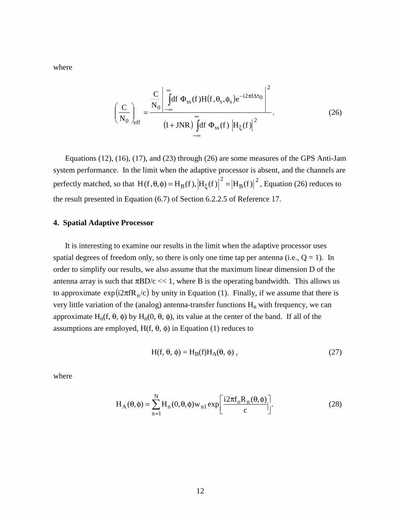
Equations (12), (16), (17), and (23) through (26) are some measures of the GPS Anti-Jam

system performance. In the limit when the adaptive processor is absent, and the channels are

perfectly matched, so that 2B

2B )f(H)f(H ),f(H),,f(H ==φθ ξ , Equation (26) reduces to

the result presented in Equation (6.7) of Section 6.2.2.5 of Reference 17.

4. Spatial Adaptive Processor It is interesting to examine our results in the limit when the adaptive processor uses

spatial degrees of freedom only, so there is only one time tap per antenna (i.e., Q = 1). In order to simplify our results, we also assume that the maximum linear dimension D of the antenna array is such that πBD/c << 1, where B is the operating bandwidth. This allows us to approximate ( )/cfRi2exp nπ by unity in Equation (1). Finally, if we assume that there is very little variation of the (analog) antenna-transfer functions Hn with frequency, we can approximate Hn(f, θ, φ) by Hn(0, θ, φ), its value at the center of the band. If all of the assumptions are employed, H(f, θ, φ) in Equation (1) reduces to H(f, θ, φ) = HB(f)HA(θ, φ) , (27) where

.c

),(Rf2iexpw),,0(H),(HN

1n

no1nnA ∑

=⎥⎦⎤

⎢⎣⎡ φθπφθ=φθ (28)

13

Likewise 2

Hξ in Equation (22) reduces to

.w)f(H)f(HN

1n

21n

2B

2∑

=ξ = (29)

If we now approximate HB(f) by a brickwall filter of bandwidth B, and substitute

Equation (27) into Equation (16), we find

( ) ( ) .e)f( df,HTAP

22B

2B

0f2iss

2ssA

200max ∫

−

τ∆π−Φφθ= (30)

Because Φss(f) is a real, non-negative definite function, it is readily seen that the right-

hand side of Equation (30) achieves its maximum when ∆τ0 = 0. Furthermore, if Equation (27) is substituted into Equation (17), along with ∆τ0 = 0, it is evident that

( ),,cossintan ssA

A

A1 φθα=⎟⎟⎠

⎞⎜⎜⎝

⎛αα=ψ∆ − (31)

where ( )ssA ,φθα is the argument of ( )ssA ,H φθ . We observe that even though the peak of the crosscorrelation occurs at the correct delay τ=τ̂ , the adaptive processor may introduce a carrier-phase error, as given by Equation (31).

Finally, if we use ∆τ0 = 0 and substitute Equations (27) and (29) into Equation (26), we

obtain for the signal-to-interference ratio when the noise is white, the result

0eff0

TNCSIR ⎟⎟

⎠

⎞⎜⎜⎝

⎛= , (32)

14

where

( ).

w)JNR1(

)f( df,HNC

NC

N

1n

21n

2B

2Bss

2ssA

0

eff0 ∑

∫

=

−

+

Φφθ⎟⎟⎠

⎞⎜⎜⎝

⎛

=⎟⎟⎠

⎞⎜⎜⎝

⎛ (33)

Typically, the system bandwidth B is sufficiently large that the integral over Φss in the numerator is very close to unity (see Equation (13)). Furthermore, in a well-designed adaptive processor, the JNR after adaptation is usually less than unity, so (1 + JNR) can often be approximated by unity. Thus, the result for the SIR becomes quite simple.

5. Summary and Discussions We have derived results for the output crosscorrelation function, signal-to-interference

ratio, the jammer-to-noise ratio, and the carrier-phase and code-delay errors at the output (point D in Figure 1) of the crosscorrelator, in the code-tracking loop of an adaptive GPS receiver, for the case when the inter-element spacings are sufficiently large that mutual coupling between the antennas in the array can be neglected.

It would be desirable if one did not need to numerically calculate the value ∆τ0 at which

( )( )τ̂ZE s achieves its maximum. We have studied this point, and found [19] that if one uses a constrained algorithm (such as constrained, minimum variance, where the array is constrained to point a receive beam in the direction of the GPS satellite) there is very little error in the code delay, so that one can use the approximation ∆τ0 = 0 in Equations (24) and (26). However, when an unconstrained algorithm (e.g., simply minimizing the output power) is used to calculate the adaptive weights, one finds that the location of the maximum of

( )[ ]τsZE is often displaced from the correct value ( τ=τ̂ , or ∆τ = 0), so that using the approximation ∆τ = 0 in Equations (24) or (26) underestimates the SIR, because the peak value of ( )sZE has shifted away from τ=τ̂ .

15

A MATLAB code has been developed to calculate all of the performance measures presented here for GNSS PN (pseudonoise) codes, such as C/A, P(Y) and the BOC (binary offset carrier) codes such as M-Code and Galileo [17]. The results are applicable to any number of jammers, each with an arbitrary power spectral density. However, because the results are jammer/GPS satellite scenario dependent, it is not instructive to present them here. That is, one obtains different answers for each set of jammer locations and power spectra and measured set of antenna/RF hardware/channel mismatch transfer functions Hn(f , θ, φ), so it is difficult to state any general conclusions.

List of References

1. Monzingo, R., and T. Miller, “Introduction to Adaptive Arrays,” Wiley, New York,

1980. 2. Compton, R., “Adaptive Antennas,” Englewood Cliffs, Prentice Hall, New Jersey,

1988. 3. Hudson, J., “Adaptive Array Principles,” Peter Peregrinus, London, 1989. 4. VanVeen, B., “Minimum Variance Beamforming,” in S. Haykin and A. Steinhardt

(Eds.), “Adaptive Radar Detection and Estimation,” Wiley, New York, 1992. 5. Gabriel, W., “Adaptive Arrays – An Introduction,” Proc. IEEE, Vol. 64, p. 239, 1976. 6. Klemm, R., “Space-Time Adaptive Processing,” IEEE, London, 1999. 7. Paulraj, A. J., and C. B. Papadias, “Space-Time Processing for Wireless

Communications,” IEEE Signal Processing Magazine, pp. 49-83, November 1997. 8. Frost, O., “An Algorithm for Linearly-Constrained Adaptive Array Processing,”

Proc. IEEE, Vol. 60, pp. 926-935, 1972. 9. Widrow, B., and S. Stearns, “Adaptive Signal Processing,” Prentice Hall, 1985. 10. Clarkson, P., “Optimal and Adaptive Signal Processing,” CRC Press, 1993. 11. Griffiths, L., “A Simple Adaptive Algorithm for Real-Time Processing in Adaptive

Arrays,” Proc. IEEE, Vol. 57, pp. 1696-1704, 1969.

16

12. Niocolau, E., and D. Zaharia, “Adaptive Arrays,” Elsevier, 1989. 13. Weiner, M., Ed., “Adaptive Antennas and Receivers,” CRC Press, Boca Raton, Florida,

2006. 14. Applebaum, S., “Adaptive Arrays,” IEEE Trans., AP-24, pp. 585-598, 1976. 15. Kaplan, E. (Ed.), “Understanding GPS: Principles and Applications,” Artech House,

Boston, Massachusetts, 1996. 16. Parkinson, B., and J. Spilker (Eds.) “Global Positioning System: Theory and

Applications,” American Institute of Aeronautics and Astronautics, Washington DC, 1996.

17. Kaplan, E., C. Hegarty, (Eds.), “Understanding GPS – Principles and Applications,”

(Second Edition), Artech House, Massachusetts, Norwood, 2006. 18. Misra, P., and P. Enge, “Global Positioning System,” Ganga-Jamuna Press,

Lincoln, Massachusetts, 2001. 19. Fante, R., and J. Vaccaro, “Wideband Cancellation of Interference in a GPS Receive

Array,” IEEE Trans. AES-36, pp. 549-564, April 2000.