performance evaluation trend forecasting based on singular...
TRANSCRIPT

Author's personal copy
Performance Evaluation 66 (2009) 173–190
Contents lists available at ScienceDirect
Performance Evaluation
journal homepage: www.elsevier.com/locate/peva
Trend forecasting based on Singular Spectrum Analysis of trafficworkload in a large-scale wireless LANI
George Tzagkarakis, Maria Papadopouli ∗, Panagiotis TsakalidesDepartment of Computer Science, University of Crete, GreeceInstitute of Computer Science, Foundation for Research and Technology-Hellas P.O. Box 1385, 711 10 Heraklion, Crete, Greece
a r t i c l e i n f o
Article history:Received 30 January 2008Received in revised form 1 June 2008Accepted 24 October 2008Available online 12 November 2008
Keywords:Traffic load modelingTraffic load forecastingSingular spectrum analysisWireless networks
a b s t r a c t
Network traffic load in an IEEE802.11 infrastructure arises from the superposition oftraffic accessed by wireless clients associated with access points (APs). An accurate loadcharacterization can be beneficial in modeling network traffic and addressing a variety ofproblems including coverage planning, resource reservation and network monitoring foranomaly detection. This study focuses on the statistical analysis of the traffic loadmeasuredin a campus-wide IEEE802.11 infrastructure at each AP.Using the Singular Spectrum Analysis approach, we found that the time-series of traffic
load at a given AP has a small intrinsic dimension. In particular, these time-series can beaccurately modeled using a small number of leading (principal) components. This provedto be critical for understanding the main features of the components forming the networktraffic.Statistical analysis of leading components has demonstrated that even a few first
components form the main part of the information. The residual components capture thesmall irregular variations, which do not fit in the basic part of the network traffic and can beinterpreted as a stochastic noise. Based on these properties, we also studied contributionsof the various components to the overall structure of the traffic load of an AP and itsvariation over time.Finally, we designed and evaluated the performance of a traffic predictor for the
trend component, obtained by projecting the original time-series on the set of leadingcomponents.
© 2008 Elsevier B.V. All rights reserved.
1. Introduction
Wireless networks are increasingly being deployed to provide Internet access in airports, universities, corporations,hospitals, residential, and other public areas. Furthermore, there is a growth in peer-to-peer, streaming, and VoIP traffic overthe wireless infrastructures [1,2]. Wireless Local Area Networks (WLANs) have more vulnerabilities and bandwidth/latencyconstraints than their wired counterparts. The bandwidth utilization at an AP can impact the performance of the wirelessclients in terms of throughput, delay, and energy consumption. For quality of service provision, capacity planning, loadbalancing, and network monitoring, it is critical to understand the traffic characteristics. For this purpose, the design ofaccurate models of the network and client activity are critical. In addition, traffic models can assist in detecting abnormaltraffic patterns (e.g., due to malicious attacks, AP or client misconfigurations and failures).
I This work was supported by the Greek General Secretariat for Research and Technology under Programs 5ENE∆-Code 03ED69 Regional of Crete,Crete-Wise KP-18 (K5Σ 00126) and 05NON-EU-238, and the European Commission (contracts MTKD-CT-2005-029791 and MIRG-CT-2005-029186).∗ Corresponding author at: Institute of Computer Science, Foundation for Research and Technology-Hellas P.O. Box 1385, 711 10Heraklion, Crete, Greece.E-mail addresses:[email protected], [email protected] (M. Papadopouli).
0166-5316/$ – see front matter© 2008 Elsevier B.V. All rights reserved.doi:10.1016/j.peva.2008.10.010

Author's personal copy
174 G. Tzagkarakis et al. / Performance Evaluation 66 (2009) 173–190
One of the most intriguing aspects of the traffic demand modeling in WLANs is its intrinsic multi-level, spatio-temporalnature, namely, the different spatial scales (e.g., infrastructure-wide, AP-level or client-level) and time granularities, suchas packet-level, flow-level and session-level. While there is a rich literature characterizing traffic in wired networks [4–6],there are only a few studies available examining wireless traffic load [1,2,9,10,27–30].In a recent work [7,8], two key structures in aWLAN, namely, the session of a client and the traffic flows generatedwithin
that session by that client,weremodeled in both spatial and temporal dimensions, and their dependencies and interrelationswere examined.Admission control and load-balancing algorithms can benefit from short-term forecasting of traffic load at hotspots.
However, such traffic predictions are challenging and suffer from large prediction errors due to the high variability [9,10]. These studies analyzed the traffic at hotspot APs and evaluated traffic forecasting algorithms based on recent history,periodicities, and number and type of flows. Specifically, the traffic load at APs was modeled using variants of the MovingAverage and Autoregressive Moving Average models, resulting in simple forecasting methods. This paper extends theseresearch efforts. To the best of our knowledge, this is the first study in characterizing statistically wireless traffic load usingnon-linear time-series analysis techniques.This research analyzes data collected using the SimpleNetworkManagement Protocol (SNMP) froma large-scalewireless
infrastructure [11] using a lightweight acquisition methodology. SNMP is the most widely-available monitoring servicein wireless platforms. Any AP in the market supports monitoring using SNMP, so it is important to understand howmuch operators and researchers can learn from SNMP data. Furthermore, this type of data is the most appropriate one tounderstand daily and long-term trends in the usage of wireless networks. This paper makes use of SNMP data for analyzingtraffic characteristics, such as total load and periodicities.To achieve a deeper understanding of the main features of traffic measurements, we employ a non-linear time-series
analysis [12,3]. At the same time, due to the complicated structure of a traffic series, traditional algorithms of non-linearanalysismay not estimate reliably the analyzed time-series. However, after filtering out a high-frequency component, whichcan be considered as a noisy part, we expect to obtain a more accurate estimation of the embedding dimension of theunderlying process. Motivated by this observation, in this study, we analyze traffic series by decomposing them in twocomponents, namely, a low-frequency and a high-frequency one, using Singular Spectrum Analysis (SSA).SSA [14] belongs to the general category of Principal Component Analysis (PCA) methods [13], which apply a linear
transformation of the original data space into a feature space, where the data set may be represented by a reduced numberof ‘‘effective’’ features while retaining most of the information content of the data. The SSA method is very efficient for theanalysis of time-series corresponding to an arbitrary process. In a recent work [15], SSA was used to analyze the dynamicsof traffic obtained at an intermediate-scale wired LAN. To the best of our knowledge, this is the first study that applies SSAon the analysis of traffic from a WLAN.This paper employs SSA to explore the intrinsic dimensionality and structure of the time-series corresponding to the
traffic load at a given AP, using data collected from a campus-wide WLAN infrastructure. To investigate the nature of thisdimensionality, we introduce the notion of eigenloads. Derived from the implementation of SSA on a given traffic load series,an eigenload is a time-series that captures a particular source of temporal variability. Each traffic load series can be expressedas a weighted sum of eigenloads, where the weights are proportional to the extent to which each eigenload is present in thegiven traffic load series.We show that traffic eigenloads in a WLAN fall into two natural classes:
- deterministic eigenloads, which capture the slow-varying trends in the traffic load series, and- noise eigenloads, which account for traffic fluctuations appearing to have relatively time-invariant properties.
By categorizing eigenloads in this manner, we obtain a significant insight into the intrinsic properties of the traffic loadseries. In particular, we find that each time-series can be approximated well by only a small number of eigenloads, whichconstitute its ‘‘feature set’’. Furthermore, these features vary in a predictable way as a function of the amount of trafficcarried in the time-series. We show that the largest traffic load series, i.e., the series with the highest mean traffic load, areprimarily deterministic. On the other hand, traffic load series of moderate size are generally comprised of noisy features.Motivated by the observation that the deterministic part of the traffic load series presents a slow variation in time and
carries the main part of the information content, we design a predictor that performs trend forecasting at a larger than anhourly time-scale. This forecasting algorithm is based on the modeling of the traffic-series using a linear model of order p,whose coefficients (weights) are estimated using the Normalized Least Mean Squares (NLMS) approach.The paper is organized as follows: Section 2 describes the wireless infrastructure at the University of North Carolina
at Chapel Hill (UNC) and the data acquisition process. In Section 3, we present the basic concept of the SSA approach. Weapply this method on our traffic measurements and analyze the leading components, which are responsible for the mainpart of the network’s traffic, and the residual components, which can be represented as irregular variations of the data.Section 4 provides a statistical modeling for a set of traffic load series, then applies SSA to these time-series, and presentsthe low-dimensionality property. Section 5 presents the classification of the eigenloads in two classes and focuses on thecharacteristics of the decomposition of traffic load series into their constituent eigenloads. Section 6 describes the design ofa traffic predictor for the trend component of the original time-series and evaluates its performance by applying it on thetime-series containing the amount of bytes received and sent, as well as, the aggregate amount of traffic, from all clientsthat were associated with a particular AP. Finally, Section 7 summarizes our main results and discusses future work plans.

Author's personal copy
G. Tzagkarakis et al. / Performance Evaluation 66 (2009) 173–190 175
2. Background
The IEEE802.11 infrastructure at UNC provides coverage for the 729-acre campus and a number of off-campusadministrative offices. The university has 26.000 students, 3.000 faculty members and 9.000 staff members. Undergraduatestudents (16.000) are required to own laptops, which are generally able to communicate using the campuswireless network.A total of 488 APs were part of the campus network at the start of our study. These APs belong to three different series of theCisco Aironet platform: the state-of-the-art 1210 Series (269 APs), the widely deployed 350 Series (188 APs) and the older340 Series (31 APs).The data was collected using SNMP for polling every AP on campus every five minutes. First, the data collection system
was implemented using a nonblocking SNMP library for polling each wireless access point (AP) precisely every five minutesin an independent manner. This eliminates any extra delays due to the slow processing of SNMP polls by some of the slowerAPs. The system ran in a multiprocessor system and the CPU utilization in each of the three processors we employed neverexceeded 70%. Second, our characterization of the workload of the APs is derived only from those clients associated withthe AP at polling time.The data collection took place between 9:09 a.m. September 29th, 2004 and 12:00 a.m. November 30th, 2004. The total
number of polling operations during the 63 days was 8.247.479. The data collection system ran flawlessly for the entireperiod, but APs were sometimes unresponsive. This is generally due to maintenance down-times, reboots, or overloads. Ifan AP did not respond to a poll, the data collection system tried again 5 s later (and if necessary, again after 10 s and 15 s).It is therefore unlikely that datagram losses created holes in our dataset.Based on the SNMP trace for each AP,we produced a time series of its traffic load at hourly intervals. This traffic is the total
amount of bytes received and sent from all clients that were associated with the AP at that time interval. In the rest of thepaper, depending on the mathematical expression, we will use two notations for these time series. Specifically, the trafficof the AP i during the h-th hour of day d (h ∈ {1, . . . , 24}, d ∈ {1, . . . , 63}), that corresponds to time t , is Ti(h, d) = Xi(t).
3. Singular Spectrum analysis of a time-series
Singular Spectrum analysis (SSA) is a method suitable for extracting information from short and noisy time series. Itunravels the information embedded in the delay-coordinate phase space by decomposing the sequence into elementarypatterns of behavior in time and spectral domains, that help separating the time series into statistically independentcomponents, which can be classified as trends and deterministic oscillations (or noise).SSA looks for structures in a time series by doing an eigendecomposition of the so-called lagged covariance matrix. This
approach is useful in non-linear system analysis, because as opposed to other time-series analysis techniques, we do nothave to choose the structure functions a priori, but instead, the data lets themselves to choose the temporal structures.Time-series corresponding to wireless traffic load are often short and contain typically peaks on top of a more regular
background. Besides, these series often have both regular (periodic) and irregular (noisy) aspects, which may be present indifferent spatial and temporal scales. Thus, the need for combining a deterministic with a stochastic modeling approach isnecessary, motivating the use of the SSA approach. The following paragraphs describe the modeling process step by stepand apply it on randomly selected time-series corresponding to several hotspot APs of our dataset.
3.1. Introduction to SSA
The SSA is applied to the analysis of time-series corresponding to an arbitrary signal x(t), with t > 0. The standard SSAconsists of four main steps:
(i) Transformation of the one-dimensional time-series into a trajectory (Hankel) matrix(ii) Singular Value Decomposition (SVD) of the Hankel matrix(iii) PCA and selection of the dominant features by grouping the SVD components(iv) Reconstruction of the original time-series using the selected features (inverse Hankelization by diagonal averaging)
Let X = {xj}Nj=1 denote the samples of the time-series and L (1 < L < N) be an integer, indicating the (caterpillar) windowlength. The transformation step forms K = N − L + 1 lagged vectors Xk = {xk, . . . , xk+L−1}T, 1 ≤ k ≤ K . The trajectoryHankel matrix of the time-series X is of dimension L× K and has the following form:
H = [X1 X2 · · · XK ]. (1)
The trajectory space is defined as the linear space spanned by the columns of H.After the above Hankelization process, the SSA method performs an SVD of the matrix C = HHT. Let λ1 ≥ · · · ≥ λL be
the eigenvalues of C, which give the energy attributable to the respective principal component, and r = max{i : λi > 0}.Let U1, . . . ,Ur denote the corresponding eigenvectors (principal components) and Vj = HTUj/
√λj, j = 1, . . . , r , the set of
factor vectors, which capture the temporal variation common to all lagged vectors along the j-th principal axis. We refer tothe set {Vj}rj=1 as the set of eigenloads of X .Since the principal axes are in order of contribution to the overall energy, V1 captures the strongest temporal trend
common to all lagged vectors, V2 captures the next strongest trend and so on. If we denote Hj =√λjUjV Tj , the trajectory

Author's personal copy
176 G. Tzagkarakis et al. / Performance Evaluation 66 (2009) 173–190
matrix H can be written asH = H1 + · · · + Hr . (2)
By applying the inverse Hankelization process on each matrix Hj, we obtain an approximation X j of the original series X .Once the expansion given by (2) has been completed, the third step of the SSA method consists of partitioning the set of
indices I = {1, . . . , r} into s disjoint subsets, where the value of s depends on the specific application. Let I1 = {i1, . . . , im}be the first subset of indices, and HI1 = Hi1 + · · · + Him to be the approximation of the trajectory matrix H based on theindices of I1. Similarly, we have an analogous decomposition corresponding to each subset Ik, k = 2, . . . , s. Thus, we obtainthe final decomposition of the initial Hankel matrix H:
H = HI1 + · · · + HIs . (3)The last step of the SSA is the application of an inverse Hankelization process on the approximation matrix HIk , k =
1, . . . , s, to approximate the initial time-series. This process is simply performed by averaging the elements ofHIk , which areplaced on the same anti-diagonal, that is, the elements hIk
ij with i+j = constant. LetXIk denote the time-series reconstructed
using the matrix HIk . Then, the j-th component of XIk , xIkj , is given by: xIkj = mean {elements of H
Ik which are placed onthe j-th anti-diagonal}.1 Thus, the result of SSA is an expansion of the original time-series into a sum of s series,
X = XI1 + · · · + XIs , (4)where XIk is the time-series reconstructed using the matrix HIk . For instance, the case s = 2 can be interpreted as aproblem of separating a signal from a noise component. The performance of themethodmainly depends on two parameters,namely, the selection of the window length L and the partitioning of the positive eigenvalues. In the following, we describeprocedures for the specification of these parameters, when using SSA for WLAN traffic workload analysis.
3.2. Estimation of the window length L
The selection of a suitable window length, L, is crucial for an increased accuracy of the SSA. The value of L is computed,such that the points of different lagged vectors, Xk, Xl (k 6= l), can be considered as linearly independent. In our context,for an arbitrary AP, the window length L is chosen to be equal to the correlation length (time lag), i.e., when the sampleauto-correlation function
C(L) =
N∑j=1(xj+L − x)(xj − x)
N∑j=1(xj − x)2
, (5)
crosses for the first time the confidence interval corresponding to the white Gaussian noise. In this case, the lagged vectorsof length L can be considered to be independent, which enables each vector to be analyzed separately. In (5), x denotes thearithmetic mean of the time-series X .Fig. 1 presents the aggregate traffic load series and the values of the sample auto-correlation function as a function of
the window length L (time lag), together with the confidence interval corresponding to the white Gaussian noise, for an APof our dataset. As shown, the auto-correlation function first crosses the confidence interval for L = 7, that is, the selectedwindow length should be equal to 7.In the following two subsections, we describe the procedure for partitioning the set of the r eigentriples {λj, Uj, Vj}rj=1
into s disjoint subsets. For convenience, we focus on the case that the eigentriples are divided in two classes, namely, theprincipal and the residual eigentriples (i.e., s = 2).
3.3. Analysis of leading components
As it was mentioned before, the eigenvalues given by applying an SVD on the trajectory matrix H can be used to select aset of feature components for the reconstruction of the original time-series. In particular, the ratio
Ri =λiL∑j=1λj
(6)
is used to estimate the energy contribution (in decreasing order) of the i-th principal component in the analyzed time-series,which can be represented as the fraction of the information content related to that (single) component.Fig. 2 shows the contribution of the eigenvalues corresponding to the aggregate traffic series of the 9-th AP in our dataset,
for two different window lengths, namely, the window length L1 = 7 given by the auto-correlation function (5), and
1 The first anti-diagonal is simply the element hIk11 .

Author's personal copy
G. Tzagkarakis et al. / Performance Evaluation 66 (2009) 173–190 177
Fig. 1. Traffic load series and sample auto-correlation function for X9(t).
Fig. 2. Percentage contribution of the eigenvalues for X9(t): (a) L = 7, (b) L = 14.
L2 = 14. This information permits the estimation of the number of principal components which effectively contributeto the information content of the time-series. As it can be seen, only the first few principal components are responsible forthe main part of the traffic information, that is, the part that maintains a high energy content.For simplicity, we are interested in grouping the principal components in two subsets, namely, a subset I1, containing
the eigenvalueswhich are responsible for the reconstruction of a slow varying (trend) component of the original time-series,and a subset I2, which is related to its ‘‘noisy’’ part. In the standard SSA approach, this partition is performed based on asignal processing point of view. In particular, the subset I1 consists of the eigenvalues λj whose corresponding eigenvectorsUj have slow varying sequences of elements, that is, the contribution of harmonics with low frequencies into their Fourierexpansion is high. Similarly, the subset I2 consists of those eigenvalues, for which the contribution of harmonics with highfrequencies into the Fourier expansion of their corresponding eigenvectors is high. In both cases, the contribution can bemeasured using the periodogram [16] of each eigenvector.In our study, instead of following this procedure, the partition of the eigenvalues is based on a statistical criterion,
in order to take into account the uncertainty of the underlying statistical model. In particular, the subset I1 of principalcomponents will consist of those eigenvalues for which the reconstructed time-series has a statistical distribution of thetraffic measurements similar to the distribution of the original time-series. Let p(x) denote the probability density function(PDF), which best fits the traffic load series of a given AP. Then, a leading component belongs to I1, if the PDF of thecorresponding reconstructed series, p(x), is close to p(x), where the ‘‘closeness’’ is measured using the χ2 test [17]. In this
Author's personal copy
178 G. Tzagkarakis et al. / Performance Evaluation 66 (2009) 173–190
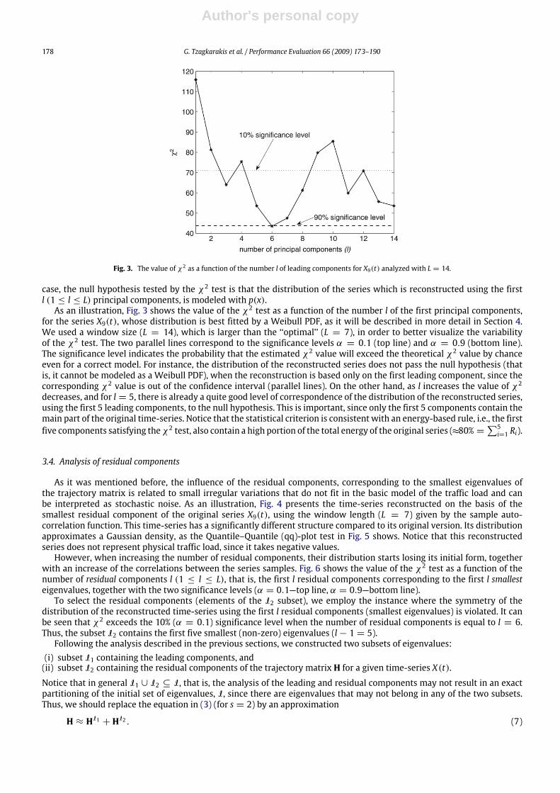
Fig. 3. The value of χ2 as a function of the number l of leading components for X9(t) analyzed with L = 14.
case, the null hypothesis tested by the χ2 test is that the distribution of the series which is reconstructed using the firstl (1 ≤ l ≤ L) principal components, is modeled with p(x).As an illustration, Fig. 3 shows the value of the χ2 test as a function of the number l of the first principal components,
for the series X9(t), whose distribution is best fitted by a Weibull PDF, as it will be described in more detail in Section 4.We used a window size (L = 14), which is larger than the ‘‘optimal’’ (L = 7), in order to better visualize the variabilityof the χ2 test. The two parallel lines correspond to the significance levels α = 0.1 (top line) and α = 0.9 (bottom line).The significance level indicates the probability that the estimated χ2 value will exceed the theoretical χ2 value by chanceeven for a correct model. For instance, the distribution of the reconstructed series does not pass the null hypothesis (thatis, it cannot be modeled as a Weibull PDF), when the reconstruction is based only on the first leading component, since thecorresponding χ2 value is out of the confidence interval (parallel lines). On the other hand, as l increases the value of χ2decreases, and for l = 5, there is already a quite good level of correspondence of the distribution of the reconstructed series,using the first 5 leading components, to the null hypothesis. This is important, since only the first 5 components contain themain part of the original time-series. Notice that the statistical criterion is consistent with an energy-based rule, i.e., the firstfive components satisfying theχ2 test, also contain a high portion of the total energy of the original series (≈80% =
∑5i=1 Ri).
3.4. Analysis of residual components
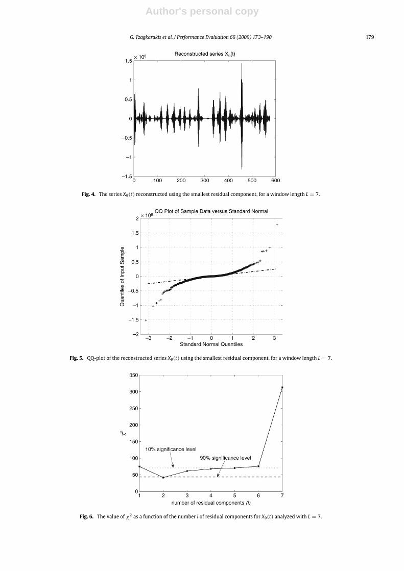
As it was mentioned before, the influence of the residual components, corresponding to the smallest eigenvalues ofthe trajectory matrix is related to small irregular variations that do not fit in the basic model of the traffic load and canbe interpreted as stochastic noise. As an illustration, Fig. 4 presents the time-series reconstructed on the basis of thesmallest residual component of the original series X9(t), using the window length (L = 7) given by the sample auto-correlation function. This time-series has a significantly different structure compared to its original version. Its distributionapproximates a Gaussian density, as the Quantile–Quantile (qq)-plot test in Fig. 5 shows. Notice that this reconstructedseries does not represent physical traffic load, since it takes negative values.However, when increasing the number of residual components, their distribution starts losing its initial form, together
with an increase of the correlations between the series samples. Fig. 6 shows the value of the χ2 test as a function of thenumber of residual components l (1 ≤ l ≤ L), that is, the first l residual components corresponding to the first l smallesteigenvalues, together with the two significance levels (α = 0.1—top line, α = 0.9—bottom line).To select the residual components (elements of the I2 subset), we employ the instance where the symmetry of the
distribution of the reconstructed time-series using the first l residual components (smallest eigenvalues) is violated. It canbe seen that χ2 exceeds the 10% (α = 0.1) significance level when the number of residual components is equal to l = 6.Thus, the subset I2 contains the first five smallest (non-zero) eigenvalues (l− 1 = 5).Following the analysis described in the previous sections, we constructed two subsets of eigenvalues:
(i) subset I1 containing the leading components, and(ii) subset I2 containing the residual components of the trajectory matrix H for a given time-series X(t).Notice that in general I1 ∪ I2 ⊆ I, that is, the analysis of the leading and residual components may not result in an exactpartitioning of the initial set of eigenvalues, I, since there are eigenvalues that may not belong in any of the two subsets.Thus, we should replace the equation in (3) (for s = 2) by an approximation
H ≈ HI1 + HI2 . (7)
Author's personal copy
G. Tzagkarakis et al. / Performance Evaluation 66 (2009) 173–190 179
Fig. 4. The series X9(t) reconstructed using the smallest residual component, for a window length L = 7.
Fig. 5. QQ-plot of the reconstructed series X9(t) using the smallest residual component, for a window length L = 7.
Fig. 6. The value of χ2 as a function of the number l of residual components for X9(t) analyzed with L = 7.

Author's personal copy
180 G. Tzagkarakis et al. / Performance Evaluation 66 (2009) 173–190
Table 1The models used in the traffic load series analysis.
Model PDF
Normal p(x) = 1σ√2πe−(x−µ)
2/(2σ 2)
log-Normal p(x) = 1xσ√2πe−(ln x−µ)
2/(2σ 2), x ∈ (0,∞)Exponential p(x) = 1
µe−x/µ
Gamma p(x) = 1bα Γ (α) x
α−1e−x/b, x ∈ [0,∞)
Rayleigh p(x) = xb2e−x
2/(2b2), x ∈ [0,∞)Weibull p(x) = bα−bxb−1e−(x/α)
b, x ∈ [0,∞)
Generalized Gaussian density (GGD) p(x) = b2α Γ (1/b) e
−(|x|α)b
The application of diagonal averaging (inverse Hankelization) on both sides of (7) results in the following approximation ofthe original time-series:
X(t) ≈ XI1(t)+ XI2(t) (8)
where XI1(t) is the time-series reconstructed using the subset of leading components, which can be interpreted as the trendof X(t), and XI2(t) is the time-series reconstructed using the subset of residual components, which can be interpreted asthe ‘‘noisy’’ (high-frequency) part of X(t).
4. SSA-based traffic load series modeling and decomposition
As discussed in Section 3, we aim at applying the SSA to decompose the traffic load series of a given AP into its constituentset of eigenloads. Besides, Section 3.3maintained that the determination of themost important (leading) eigenloads is basedon the selection of a suitable statistical model, which accurately fits the distribution of the original traffic load series, to beused in the χ2 test. Thus, a statistical analysis for the selection of the best model is necessary.This section first shows that traffic load series corresponding to the total amount of bytes received (download) and sent
(upload), as well as, the aggregate amount of traffic, from all clients that are associated with a particular AP can be modeledusing PDFs belonging to different families. Then, we use the corresponding best models to show that only a small set ofeigenloads can reconstruct the original time-series accurately, while preserving its characteristic features, such as its spikes.
4.1. Statistical modeling of traffic load series
The first step in our statistical analysis is based on accurate modeling of the mode and tails of the distribution of agiven traffic load series. Since the time-series in our dataset are in general bursty, we expect that their distributions willbe modeled using non-Gaussian PDFs. Before proceeding, we assess whether the data deviate from the normal distributionusing qq-plots. Then, we determine the model that best fits the empirical distribution of the time-series by employing theso-called amplitude probability density (APD) curves, which represent the probability P(|X | > x). The APD curves give agood indication of whether or not a particular model matches our data near the mode and on the tails of the empiricaldistribution.Table 1 indicates the candidate statistical models used in our analysis. The statistical fitting of each one of the 19 time-
series constituting our dataset showed that the Gamma is the dominant distribution followed by the GGD. Fig. 7 shows theAPD curves for the aggregate traffic load series X2(t), as well as, the upload traffic and the download traffic, whose empiricaldistribution is best approximated using the GGD, Gamma and Weibull distribution, respectively.
4.2. Normalization of the traffic measurements
Due to the nature of wireless traffic, the traffic load of a particular AP iwithin hour t , Xi(t), exhibits spikes that are veryhard to predict. Fig. 8 shows the traffic load series and its normal probability plot for the third hotspot AP in our dataset,X3(t). Its bursty behavior is clear, and the marginal distribution is non-Gaussian. Thus, before proceeding to handle the datamore efficiently, we normalize them so that their distribution resembles the normal distribution, by employing a suitabletransformation. Normal distributions can be handled more effectively. Besides, such a transformation can reduce the effectof those high local spikes on the forecasting performance. Unfortunately, in general, the choice of the best transformation isnot obvious.There is a family of power transformations to make the marginal distributions resemble a Gaussian-like density, namely
the Box–Cox power transformations, defined only for positive data values. The existence of zero values in the trace does not

Author's personal copy
G. Tzagkarakis et al. / Performance Evaluation 66 (2009) 173–190 181
(a) APD curves of the time-series X2(t). (b) APD curves of the download time-series.
(c) APD curves of the upload time-series.
Fig. 7. APD curves for the time-series corresponding to the traffic of AP 2: (a) aggregate traffic, (b) download trafic, (c) upload traffic.
pose any problem, since a constant can always be added. The Box–Cox power transformation is given by [18]:
x(ρ) =
xρ − 1ρ
, ρ 6= 0
ln(x), ρ = 0.(9)
Given the time-series X = {xj}Nj=1, one way to select the optimal power ρ is to maximize the log-likelihood function
f (X, ρ) = −N2ln
[N∑j=1
(xj(ρ)− x(ρ))2
N
]+ (ρ − 1)
N∑j=1
ln(xj(ρ)), (10)
where
x(ρ) =1N
N∑j=1
xj(ρ).
Let Yi(t) = Xi(t; ρopt) denote the transformed version of the original time-series Xi(t) using the optimal value of ρ (ρopt ).Fig. 9 shows the Box–Cox transformed version (Y3(t)) of the original series X3(t), as well as, themean and standard deviationper hour-of-day (h(t) ∈ {1, . . . , 24}) of the original series X3(t). It is apparent that the effect of the large spikes, present
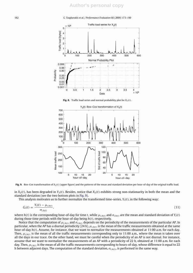
Author's personal copy
182 G. Tzagkarakis et al. / Performance Evaluation 66 (2009) 173–190
Fig. 8. Traffic load series and normal probability plot for X3(t).
Fig. 9. Box–Cox transformation of X3(t) (upper figure) and the patterns of the mean and standard deviation per hour-of-day of the original traffic load.
in X3(t), has been degraded in Y3(t). Besides, notice that X3(t) exhibits strong non-stationarity in both the mean and thestandard deviation (see the two bottom plots in Fig. 9).This analysis motivates us to further normalize the transformed time-series, Yi(t), in the following way:
Gi(t) =Yi(t)− µi,h(t)
σi,h(t), (11)
where h(t) is the corresponding hour-of-day for time t , while µi,h(t) and σi,h(t) are the mean and standard deviation of Yi(t)during those time periods with the hour-of-day being h(t), respectively.Notice that the computation of µi,h(t) and σi,h(t) depends on the periodicity of the measurements of the particular AP. In
particular, when the AP has a diurnal periodicity (24 h),µi,h(t) is the mean of the traffic measurements obtained at the samehour-of-day h(t). Assume, for instance, that we want to normalize the measurements obtained at 11:00 a.m. for each day.Then, µi,h(t) is the mean of all the traffic measurements corresponding only to 11:00 a.m., where the mean is taken overall the days in our trace. On the other hand, we must be careful when the periodicity of an AP is not diurnal. For instance,assume that we want to normalize the measurements of an AP with a periodicity of 22 h, obtained at 11:00 a.m. for eachday. Then,µi,h(t) is the mean of all the traffic measurements corresponding to hours-of-day, whose difference is equal to 22h between adjacent days. The computation of the standard deviation, σi,h(t), is performed in the same way.
Author's personal copy
G. Tzagkarakis et al. / Performance Evaluation 66 (2009) 173–190 183
Fig. 10. (a) Percentage contribution of the eigenvalues and (b) χ2 test values for G9(t) (L = 33).
Fig. 11. SSA approximation using the first 6 leading components for: (a) the normalized series G9(t), (b) the original series X9(t).
It is also important to notice that after the above transformations, the model that best fits the empirical distribution ofGi(t) and the optimal window length L, given by the sample auto-correlation function, may change.
4.3. Low-dimensionality of traffic load series
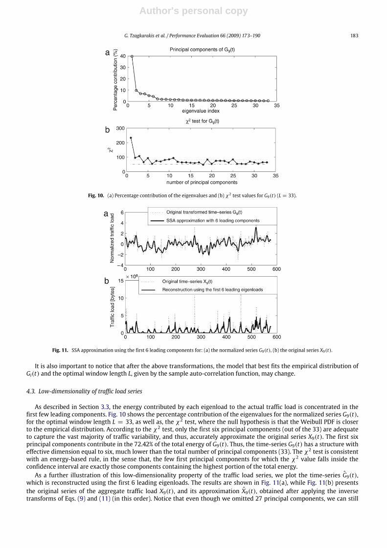
As described in Section 3.3, the energy contributed by each eigenload to the actual traffic load is concentrated in thefirst few leading components. Fig. 10 shows the percentage contribution of the eigenvalues for the normalized series G9(t),for the optimal window length L = 33, as well as, the χ2 test, where the null hypothesis is that the Weibull PDF is closerto the empirical distribution. According to the χ2 test, only the first six principal components (out of the 33) are adequateto capture the vast majority of traffic variability, and thus, accurately approximate the original series X9(t). The first sixprincipal components contribute in the 72.42% of the total energy of G9(t). Thus, the time-series G9(t) has a structure witheffective dimension equal to six, much lower than the total number of principal components (33). The χ2 test is consistentwith an energy-based rule, in the sense that, the few first principal components for which the χ2 value falls inside theconfidence interval are exactly those components containing the highest portion of the total energy.As a further illustration of this low-dimensionality property of the traffic load series, we plot the time-series G9(t),
which is reconstructed using the first 6 leading eigenloads. The results are shown in Fig. 11(a), while Fig. 11(b) presentsthe original series of the aggregate traffic load X9(t), and its approximation X9(t), obtained after applying the inversetransforms of Eqs. (9) and (11) (in this order). Notice that even though we omitted 27 principal components, we can still

Author's personal copy
184 G. Tzagkarakis et al. / Performance Evaluation 66 (2009) 173–190
Fig. 12. SSA approximation using the first K leading components for: (a) the normalized upload series (K = 13), (b) the normalized download series(K = 5), of the 9-th AP.
capture most of the important characteristics of the original series X9(t), such as the locations of its spikes. Fig. 12 showsthe approximation results using the set of leading components for the normalized upload and download traffic-series ofthe 9-th AP. In particular, Fig. 12(a) illustrates the normalized upload traffic-series, analyzed with a window size L = 35,along with its approximation using the first 13 leading components, while in Fig. 12(b), we plot the normalized downloadtraffic-series, analyzed with a window size L = 32, along with its approximation using the first 5 leading components. Fromthe above figures it is clear that the SSA approach is suitable for the approximation not only of the aggregate traffic loadseries, but also of its two additive components, namely the upload and download traffic. Notice that in general these threetime-series (upload, download, aggregate) are analyzed using different window sizes, L, and statistical distributions.We do not expect to capture accurately the exact height of a spike, using only such a small number of eigenloads. Our
goal is to illustrate that the main information content of a traffic load series in our dataset is mainly due to the contributionof a small number of features (eigenloads). Thus, we can understand better the intrinsic behavior of actual traffic by studyingthe behavior of a small set of eigenloads, which appear to have a better structure compared with the original traffic loadseries, as described in the next section.
5. Structure of the eigenloads
The statistical analysis of the traffic load series presented in the previous section underscores the central role of theeigenloads in understanding the intrinsic properties of a traffic load series obtained in a large-scale WLAN, such as thenetwork considered in our study. Thus,we are interested in describing the two types of eigenloads, namely, the deterministic(slow-varying) and the noisy one.
5.1. Categorization of eigenloads
In Section 3.1, we defined the set of eigenloads {Vj}rj=1 as a function of the set of eigenpairs {λj, Uj}rj=1. The value of λj
is proportional to the extend to which its corresponding principal component Uj contributes to the j-th eigenload of thetime-series X(t). Thus, before the categorization of the eigenloads, we start by inspecting the set of principal components{Uj}rj=1.The principal components of the traffic load series (upload, download, and aggregate) in our dataset for each one of the
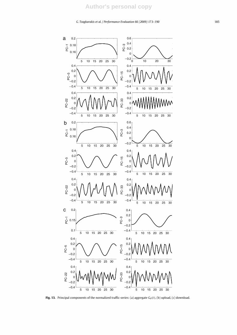
19 hotspot APs appear to have the same behavior. In particular, we found that a principal component whose correspondingeigenvalue is of high magnitude is slow-varying, whereas as the magnitude of an eigenvalue decreases, its correspondingeigenvector oscillates more andmore. As an illustration of this behavior, Fig. 13 shows a subset of the principal componentsfor the normalized aggregate traffic-series G9(t), as well as, its corresponding upload and download traffic-series, where theprincipal components are ordered in decreasing order with respect to their corresponding eigenvalue.The categorization of the set of eigenloads is performed in a heuristic way. In particular, we expect that the eigenloads
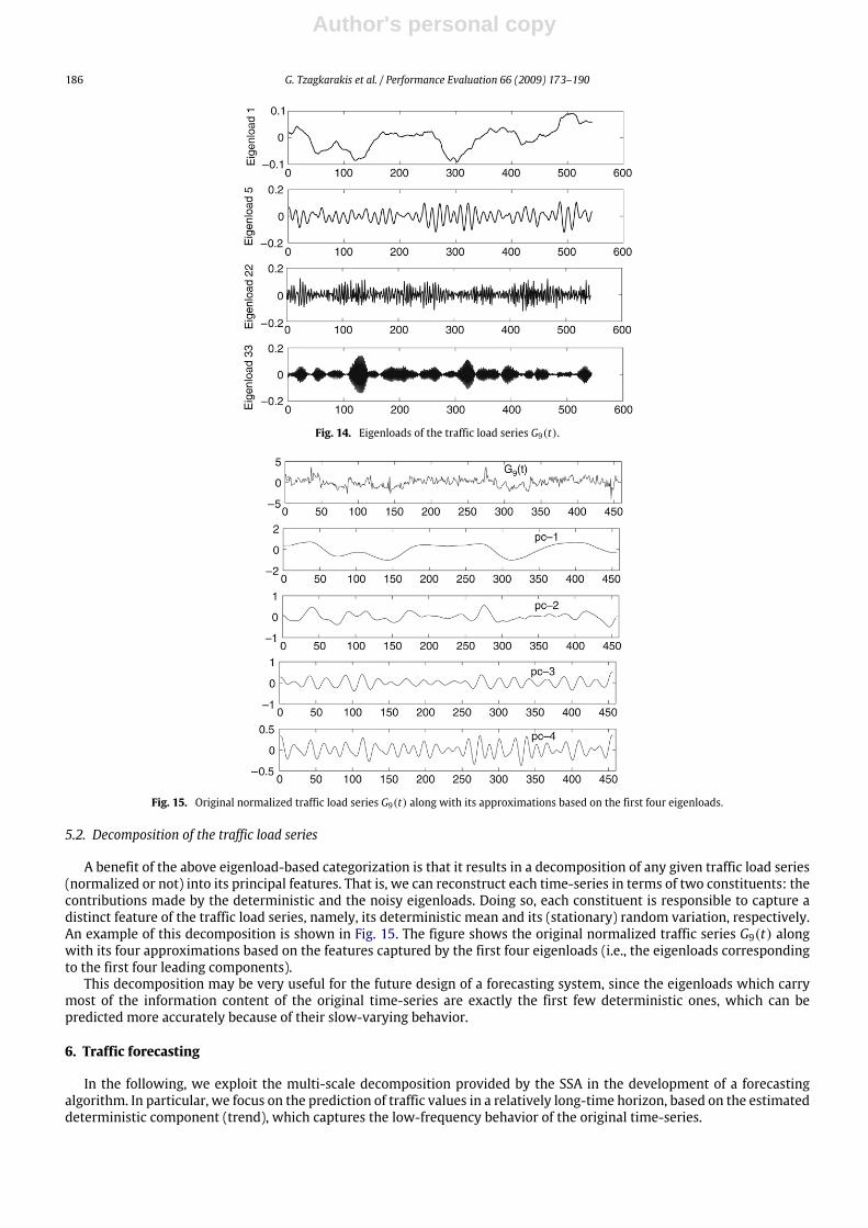
will present a similar behavior as the principal components, since they are obtained as projections of the trajectorymatrixHon them. Thus, we divide the eigenloads in two classes: (i) the deterministic, slow-varying eigenloads, which are simply theprojections of H on slow-varying principal components, and (ii) the noisy eigenloads, which result by projecting H on thehigh-frequency principal components. As an example, Fig. 14 shows the eigenloads given by the projection of the trajectorymatrix of the normalized time-series G9(t) on the principal components 1, 5, 22 and 33. It is clear that the eigenloads 1 and5 can be considered as deterministic, while the eigenloads 22 and 33 belong to the noisy class.
Author's personal copy
G. Tzagkarakis et al. / Performance Evaluation 66 (2009) 173–190 185
Fig. 13. Principal components of the normalized traffic-series: (a) aggregate G9(t), (b) upload, (c) download.
Author's personal copy
186 G. Tzagkarakis et al. / Performance Evaluation 66 (2009) 173–190
Fig. 14. Eigenloads of the traffic load series G9(t).
Fig. 15. Original normalized traffic load series G9(t) along with its approximations based on the first four eigenloads.
5.2. Decomposition of the traffic load series
A benefit of the above eigenload-based categorization is that it results in a decomposition of any given traffic load series(normalized or not) into its principal features. That is, we can reconstruct each time-series in terms of two constituents: thecontributions made by the deterministic and the noisy eigenloads. Doing so, each constituent is responsible to capture adistinct feature of the traffic load series, namely, its deterministic mean and its (stationary) random variation, respectively.An example of this decomposition is shown in Fig. 15. The figure shows the original normalized traffic series G9(t) alongwith its four approximations based on the features captured by the first four eigenloads (i.e., the eigenloads correspondingto the first four leading components).This decomposition may be very useful for the future design of a forecasting system, since the eigenloads which carry
most of the information content of the original time-series are exactly the first few deterministic ones, which can bepredicted more accurately because of their slow-varying behavior.
6. Traffic forecasting
In the following, we exploit the multi-scale decomposition provided by the SSA in the development of a forecastingalgorithm. In particular, we focus on the prediction of traffic values in a relatively long-time horizon, based on the estimateddeterministic component (trend), which captures the low-frequency behavior of the original time-series.

Author's personal copy
G. Tzagkarakis et al. / Performance Evaluation 66 (2009) 173–190 187
Table 2Optimal order p for the BRECV, BSENT and aggregate time-series of a subset of 10 AP’s.
AP index 1 2 4 6 8BRECV 21 32 22 22 12BSENT 32 80 32 30 32Aggregate 30 10 12 40 70AP index 10 11 14 16 18BRECV 12 12 22 32 32BSENT 32 32 12 32 70Aggregate 12 12 12 42 80
An initial attempt toward long-term forecasting of IP network traffic is described in [19], where a single value for theaggregate number of bytes flowing over the NSFNET is computed, and linear time-series models are used for modelingthe traffic behavior. Specifically, the time-series obtained are modeled with a low-order autoregressive integrated movingaverage (ARIMA) model, offering highly accurate forecasts for up to two years in the future. However, predicting a singlevalue for the future network-wide load could be relevant for dynamic resource allocation in small time-scales [20,21], but it isinsufficient for capacity planning purposes. In this case, it is necessary to developmodels in larger time-scales for long-termforecasting. An initial attempt to model the evolution of IP backbone traffic at large time-scales is described in [22], whichrelies on the wavelet multiresolution analysis and linear time-series models. In particular, the collected measurementsare smoothed using a wavelet decomposition in multiple scales, until the overall long-term trend is identified. Then, theforecasting of this trend component is achieved by fitting it with a low-order ARIMA model.In our work, we are interested in predicting the behavior of the trend component of the traffic load in a campus-wide
WLAN, at a larger than an hourly time-scale, for instance to predict the trend in the next few days. Our measurements comefrom a dynamic environment reflecting events that may have short or long-time effects on the observed behavior. The long-time events influence the overall long-term trend, and the main part of the variability observed. Events that may have ashort-time duration, such as link failures, usually have a direct impact on the measured traffic but their effect fades aftersome time. As a consequence, they contribute to the measured traffic-series with values which lie beyond the overall trend.Given that such events are very hard to predict, we will not attempt to model them in this paper, but we provide somedirections for future research in the last section.
6.1. Traffic predictor overview
As mentioned before, the trend component of the original (normalized) traffic-series is obtained by projecting it on theset of leading components, given by the SSA. In the following, let Gdi (t) denote the deterministic component (trend), of theoriginal normalized traffic-series Gi(t). The design of a predictor for Gdi (t) is based on its fitting with a p-th order linearmodel of the form
Gdi (t + 1) =p−1∑l=0
wt(l)Gdi (t − l), (12)
wherewt = [wt(0), wt(1), . . . , wt(p− 1)]T denotes the predictor’s weight vector at time t . Besides, let e(t) = Gdi (t + 1)−Gdi (t + 1) denote the prediction error. The Normalized Least Mean Squares (NLMS) [23] algorithm uses error feedback toupdate successively the weight vector as follows,
wt+1 = wt +µ e(t − 1)Gdi (t − 1)‖Gdi (t − 1)‖2
, (13)
where Gdi (t − 1) = [Gdi (t − 1),G
di (t − 2), . . . ,G
di (t − p)]
T and µ is a step size parameter. Notice that the error e(t − 1)is used instead of e(t) in (13), since e(t) is not available at time t (it requires the knowledge of the future value Gdi (t + 1)).Besides, the selection of µ such that 0 < µ < 2 is necessary for the convergence of the weight vector [23]. In our proposedmethod, we set µ = 0.5 and the weights of the NLMS predictor are adapted periodically, after new measurements becomeavailable in a predefined time interval.The selection of the model’s order p, is equivalent to selecting an appropriate window size in terms of the number of
samples of past traffic load, and controls the amount of traffic history measurements to be used in forecasting the futuretraffic load. In the proposedmethod, we select the value of p by fitting a family of models to a subset of Gdi (t) values (e.g. thetraffic load in the first 5 days), for several values of p, and select the optimal value of p byminimizing the Akaike InformationCriterion (AIC) [24]. Although in ourmethod this optimal value ismaintained during thewhole forecasting period, one couldalso re-estimate the optimal p in certain periods. Table 2 shows the optimal order for the time-series containing the amountof bytes received (BRECV), sent (BSENT), as well as, the aggregate traffic load, from all clients that were associated with aparticular AP, for a subset of 10 out of the 19 hotspot AP’s in our dataset. These 10 AP’s are selected as the ones for whichthe SSA approach resulted in the best statistical modeling using one of the distributions shown in Table 1.

Author's personal copy
188 G. Tzagkarakis et al. / Performance Evaluation 66 (2009) 173–190
Fig. 16. Median absolute relative prediction error E1.
We observe that for the same AP, the optimal order of the two separate traffic load series, namely the BRECV and BSENT,can be very different from each other, which is due to their different variation. Usually, the predictor’s order p increases asthe non-stationarity of the time-series increases.The proposed forecasting scheme collects the traffic load measurements at certain time intervals. These values are the
inputs for the traffic predictor. After each sampling, a prediction is made for the traffic load in the next sampling period. Thisforecast could be then used in the future management of the network’s capacity, such as in deciding whether to admit orreject new associations in a certain AP.
6.2. Evaluation of traffic load forecasting
In the following, we apply the proposed methodology to predict the trend of the traffic series corresponding to each oneof the 10 AP’s, whose indexes are shown in Table 2. In particular, we evaluate the prediction performance for the BRECV andBSENT time-series, as well as for the time-series containing the aggregate traffic load, which is simply the sum of BRECVand BSENT. These time-series contain the traffic load for a period of 58 days. The NLMS approach is employed to update theweight vector wt every two days. That is, the traffic load values in a window, whose size depends on the model’s order p,are used to predict the trend in the next two days. Then, the true measurements collected during these two days are usedfor updating the weight vector and predicting the trend for the next two days and so on.Two metrics are used for the evaluation of the forecasting performance, namely (i) the absolute relative prediction error
with respect to the true trend (we denote it by E1) and (ii) the absolute relative prediction error with respect to the truetotal traffic load (denoted by E2), which are defined as follows,
E1(t) =
∣∣∣∣∣Gdi (t)− Gdi (t)Gdi (t)
∣∣∣∣∣ , (14)
E2(t) =
∣∣∣∣∣Gi(t)− Gdi (t)Gi(t)
∣∣∣∣∣ . (15)
Fig. 16 shows the median relative prediction error E1 for the time-series of the upload (BSENT), the download (BRECV),as well as, the aggregate traffic load, for each one of the selected 10 AP’s, while Fig. 17 shows the corresponding medianrelative prediction errors E2. From the first figure we can see that the trend component can be predicted with high accuracyfor these AP’s, while the second one shows that for most of the 10 AP’s, the predicted value of the trend is relatively closeto the total traffic load, which is also an indication that the trend component carries the major part of the informationcontent of the original time-series. We expect that the forecasting performance can be improved by taking into account theresidual components, which constitute the noisy part of the original time-series and are responsible for the high-frequencyfluctuations.
7. Conclusions
In this paper, we provided an SSA-based statistical analysis of the structure of traffic load series measured in a large-scale campus-wide WLAN. First, we fitted the distribution of a given time-series containing the upload, download or theaggregate traffic load, obtained at the AP level, using an appropriate model selected from a set of pre-determined candidate

Author's personal copy
G. Tzagkarakis et al. / Performance Evaluation 66 (2009) 173–190 189
Fig. 17. Median absolute relative prediction error E2.
PDFs. Then, we applied the SSA approach in order to partition the set of principal components in two subsets, namely, thesubset of leading components and the subset of residual components.We showed that the subset of leading components is responsible for the preservation of the main information content
of the original series and thus, the intrinsic dimensionality of the traffic is highly restricted by using only the first fewleading components. Besides, we found that the eigenloads, defined using the set of leading components, present a similarbehavior across the different traffic load series. In particular, we showed that they can be categorized in two classes: (i)the deterministic, slow-varying eigenloads carrying the major information content and (ii) the noisy eigenloads, which arerelated with the irregular variations of the traffic.Based on this categorization, we decomposed the original traffic series by projecting it on each eigenload. This yielded a
considerable understanding of the structure of the traffic load series, which is analyzed in multiple frequency scales, sincethe projections on the first eigenloads give the slow-varying trend components, while the projections on the last eigenloadsgive the high-frequency content.Motivated by the common behavior of the eigenloads among the several AP’s, we exploited the slow-varying trend
components to design a traffic predictor. The results revealed an increased forecasting performance of the deterministicpart, for the traffic-series of those AP’s for which the SSA approach provided an accurate statistical modeling.As a futurework, wewill complete the design of the proposed predictor by taking into account not only the deterministic,
but also the noisy component of a given traffic-series. For this purpose, an optimal radial basis function will be trained forthe prediction of the noisy part [25].Another interesting problem is the detection of dynamical changes of the future traffic load values. In particular, the
accurate detection of transitions from a normal to an abnormal state, either due to hardware or software failure, or dueto an attack, may improve diagnosis and treatment. The multi-scale decomposition given by the SSA approach, couldbe combined with the conceptually simple and computationally very fast concept of permutation entropy [26] to detectdynamical changes in the subset of noisy eigenloads, which are responsible for the transient behavior of the traffic loadseries. Besides, to encourage further experimentation, we havemade our datasets available to the research community [31].
References
[1] T. Henderson, D. Kotz, I. Abyzov, The changing usage of a mature campuswide wireless network, in: ACM/IEEE International Conference on MobileComputing and Networking (MobiCom), Philadelphia, Sep. 2004.
[2] M. Ploumidis, M. Papadopouli, T. Karagiannis, Multi-level application-based traffic characterization in a large-scale wireless network, in: Proc. of theIEEE International Symposium on a World of Wireless, Mobile and Multimedia Networks (WoWMoM), Helsinki, Finland, June 2007.
[3] F. Anjum, M. Elaoud, D. Famolari, A. Ghosh, R. Vaidyanathan, A. Dutta, P. Agrawa, T. Kodama, Y. Katsube, Voice performance in WLan networks, anexperimental study, in: Proc. of the IEEE Conference on Global Communications (GLOBECOM), Rio De Janeiro, Brazil, Dec. 2003.
[4] W.E. Leland, M.S. Taqqu,W.Willinger, D.V.Wilson, On the self-similar nature of ethernet traffic, ACM Computer Communication Review 25 (1) (1995)202–213.
[5] W.E. Leland, W. Willinger, M.S. Taqqu, D.V. Wilson, Statistical analysis and stochastic modeling of self-similar datatraffic, in: Proc. 14th Int. TeletrafficCong., vol. 1, Antibes Juan Les Pins, France, June 1994, pp. 319–328.
[6] A. Lakhina, K. Papagiannaki, M. Crovella, C. Diot, E.D. Kolaczyk, N. Taft, Structural analysis of network traffic flows, ACM Sigmetrics, New York, June2004.
[7] F.H. Campos,M. Karaliopoulos,M. Papadopouli, H. Shen, Spatio-temporalmodeling of trafficworkload in a campusWLAN, in: 2nd annual intl.WIrelessinternet CONference (WICON’06), Boston, USA, August 2–5, 2006.
[8] M. Karaliopoulos, M. Papadopouli, E. Raftopoulos, H. Shen, On scalable measurement-driven modelling of traffic demand in large WLans, in: Proc. ofthe IEEE Workshop on Local and Metropolitan Area Networks, Princeton NJ, USA, June 10–13, 2007.
[9] M. Papadopouli, H. Shen, E. Raftopoulos, M. Ploumidis, F. Hernandez-Campos, Short-term traffic forecasting in a campus-wide wireless network, in:16th Annual IEEE Intl. Symp. on Personal Indoor and Mobile Radio Comm., Berlin, Germany, September 11–14, 2005.

Author's personal copy
190 G. Tzagkarakis et al. / Performance Evaluation 66 (2009) 173–190
[10] M. Papadopouli, E. Raftopoulos, H. Shen, Evaluation of short-term traffic forecasting algorithms inwireless networks, in: 2nd Conf. on Next GenerationInternet Design and Engineering, Valencia, Spain, April 3–5, 2006.
[11] America’s most connected campuses, http://forbes.com/home/lists/2004/10/20/04conncampland.html.[12] H.D.I. Abarbanel, Analysis of Observed Chaotic Data, Springer-Verlag, Inc, New York, 1996.[13] I.T. Jolliffe, Principal Component Analysis, Springer-Verlag, 1986.[14] N. Golyandina, V. Nekrutkin, A. Zhigljavsky, Analysis of Time Series Structure: SSA and Related Techniques, Chapman & Hall/CRC, 2001.[15] I. Antoniou, V.V. Ivanov, Valery V. Ivanov, P.V. Zrelov, Principal component analysis of network traffic measurements: The ‘‘Caterpillar’’-SSA approach,
in: VIII Int. Workshop on Advanced Computing and Analysis Techniques in Physics Research, ACAT’2002, 24–28 June 2002, Moscow Russia.[16] M.H. Hayes, Statistical Digital Signal Processing and Modeling, John Wiley & Sons, 1996.[17] P.E. Greenwood, M.S. Nikulin, A Guide to Chi-Squared Testing, John Wiley & Sons, Ltd, Canada, 1996.[18] G.E.P. Box, G.M. Jenkins, G.C. Reinsel, Time Series Analysis, Forecasting and Control, 3rd ed., Prentice Hall, Englewood Clifs, NJ, 1994.[19] N.K. Groschwitz, G.C. Polyzos, A Time Series Model of Long-Term NSFNET Backbone Traffic, in: IEEE ICC94, 1994.[20] S. Basu, A. Mukherjee, Time Series Models for Internet Traffic, in: 24th Conf. on Local Computer Networks, Oct. 1999, pp. 164–171.[21] A. Sang, S. Li, A Predictability Analysis of Network Traffic, in: INFOCOM, Tel Aviv, Israel, Mar. 2000.[22] K. Papagiannaki, N. Taft, Z.-L. Zhang, C. Diot, Long-term forecasting of internet backbone traffic, IEEE Transactions on Neural Networks 16 (5) (2005)
1110–1124.[23] M.H. Hayes, Statistical Digital Signal Processing and Modeling, John Wiley & Sons, Inc, New York, 1996.[24] P.F. Brockwell, R.A. Davis, Time Series: Theory and Methods, Springer-Verlag, New York, New York, 1998.[25] H. Leung, T. Lo, S. Wang, Prediction of noisy chaotic time series using an optimal radial basis function neaural network, IEEE Transactions on Neural
Networks 12 (5) (2001) 1163–1172.[26] Y. Cao,W.W. Tung, J.B. Gao, V.A. Protopopescu, L.M. Hively, Detecting dynamical changes in time series using the permutation entropy, Physical Review
E 70 (2004) 046217.[27] M. Papadopouli, H. Shen, M. Spanakis, Modeling client arrivals at access points in wireless campus-wide networks, in: 14th IEEE Workshop on Local
and Metropolitan Area Networks, Chania, Crete, Greece, Sep. 2005.[28] M. Papadopouli, H. Shen, M. Spanakis, Characterizing the duration and association patterns of wireless access in a campus, in: 11th EuropeanWireless
Conference, Nicosia, Cyprus, Apr. 2005.[29] G. Tzagkarakis, M. Papadopouli, P. Tsakalides, Singular Spectrum Analysis of Traffic Workload in a Large-scale Wireless LAN, in: 10th ACM/IEEE
International Symposium on Modeling, Analysis and Simulation of Wireless and Mobile Systems, Chania, Crete, Greece, Oct. 2007.[30] F. Chinchilla, M. Lindsey, M. Papadopouli, Analysis of wireless information locality and association patterns in a campus, in: IEEE INFOCOM 2004,
Hong Kong, Mar. 2004.[31] UNC/FO.R.T.H. archive of wireless traces, models and tools, http://netserver.ics.forth.gr/datatraces/.
George Tzagkarakis received the B.S. degree in Mathematics from the University of Crete (UOC), Greece, in 2002 (First in Class,Honors). At the same year he joined the Computer Science department (CSD) at the UOC for graduate studies with scholarshipsfrom the CSD and the Institute of Computer Science (ICS) of the Foundation for Research and Technology-Hellas (FO.R.T.H.).He received the M.Sc. degree in 2004 (First in Class, Honors) and he is currently pursuing the Ph.D. degree in the area ofsignal processing with applications in sensor networks. Since 2000, he has been also collaborating with the Wave PropagationGroup of the Institute of Applied and Computational Mathematics (FO.R.T.H.), while from 2002 he is a research assistant in theTelecommunications and Networks Lab (ICS). His research interests lie in the fields of statistical signal & image processing withemphasis in non-Gaussian heavy-tailed modeling, distributed signal processing for sensor networks, information theory, andapplications in image classification/retrieval and inverse problems in underwater acoustics.
Maria Papadopouli (Ph.D. Columbia University, October 2002) is an assistant professor in the Department of Computer Scienceat University of Crete, a research associate at the Institute of Computer Science, Foundation for Research and Technology-Hellas(FORTH-ICS), Greece, and an adjunct professor in Department of Computer Science at the University of North Carolina at ChapelHill (UNC-CH). From July 2002 until June 2006, she was a tenure-track assistant professor at UNC-CH (on leave from July 2004until June 2006). Her current research interests are in mobile peer-to-peer computing, wireless networks, networkmodelling andperformance analysis, and pervasive computing. In 2004 and 2005, she was awarded with an IBM Faculty Award.Maria Papadopouli and Henning Schulzrinne recently published a monograph on ‘‘Peer-to-Peer Computing for Mobile
Networks: Information Discovery and Dissemination’’, Springer, November 2008.More information about her research can be found at http://www.ics.forth.gr/mobile/.
Panagiotis Tsakalides (M’95) received the Diploma in electrical engineering from the Aristotle University of Thessaloniki,Thessaloniki, Greece, in 1990, and the Ph.D. degree in electrical engineering from the University of Southern California (USC),Los Angeles, in 1995. He is an Associate Professor of computer science at the University of Crete, Greece, and a Researcher withthe Institute of Computer Science, Foundation for Research and Technology-Hellas (FORTH-ICS), Greece. From 2004 to 2006, heserved as the Department Chairman. From 1999 to 2002, he was with the Department of Electrical Engineering, University ofPatras, Greece. From 1996 to 1998, he was a Research Assistant Professor with the Signal and Image Processing Institute, USC, andhe consulted for the U.S. Navy and Air Force. His research interests lie in the field of statistical signal processing with emphasis innon-Gaussian estimation and detection theory, and applications in wireless communications, imaging, and multimedia systems.He has coauthored over 80 technical publications in these areas, including 25 journal papers. Currently, he is the PI of ASPIRE, a1.2 MeMarie Curie Transfer of Knowledge (ToK) grant funded by the European Union to perform research on distributed signalprocessing for sensor networks. Dr. Tsakalides was awarded the IEE’s A.H. Reeve Premium in 2002 (with coauthors P. Reveliotis
and C.L. Nikias) for the paper ‘‘Scalar quantization of heavy tailed signals’’ published in the October 2000 issue of the IEE Proceedings-Vision, Image andSignal Processing.