performance constraints of distributed control loops … · distributed control loops, ... and...
TRANSCRIPT

Performance Constraints of DistributedControl Loops on Linux Systems
Andrew Boie and Dr. Douglas Niehaus
ITTC-FY2008-TR-41420-05
December 2007
Copyright © 2007:The University of Kansas2335 Irving Hill Road, Lawrence, KS 66045-7612All rights reserved.
Project Sponsor:Oak Ridge National Laboratory
Technical Report
The University of Kansas

Abstract The number of distributed applications that play important roles in industry,
commerce, and daily life is steadily increasing. The execution behavior constraints that distributed applications must meet vary widely, but those of the important sub-class, the distributed control loops, are the focus of the work described in this report. Distributed control loops have two characteristics of particular interest: (1) components of the application communicate with each other across machine boundaries, and (2) the end-to-end response time and other aspects of control loop behavior are subject to specified timing constraints. Distributed control loops have been implemented for decades, but generally using specialized computation platforms. Recent trends make supporting such control loops alongside other applications on low cost commercial off the shelf (COTS) platforms, particularly open source platforms, increasingly attractive. The viability of this approach depends crucially on which aspects of these low cost platforms constrain control loop performance, what the constraints are, and where in the system they are created. This report describes a number of experiments which explore the performance envelope of control loops on Linux using the increasingly popular RT-Patch, and which indicate areas of the system constraining the performance of control loops and thus limiting the set of distributed control loop applications which could successfully use this example target platform.
i

Table of Contents Abstract ................................................................................................................................ i Table of Contents ................................................................................................................ ii List of Figures .................................................................................................................... iv 1 Introduction...................................................................................................................... 1
1.1 The Problem of Interest ............................................................................................ 2 1.2 Our Approach............................................................................................................ 3
2 Experiment Component Software.................................................................................... 5 2.1 Datastreams............................................................................................................... 5 2.2 CLKSYNC................................................................................................................ 6 2.3 NETSPEC Control Software..................................................................................... 7 2.4 KUIM Image Processing Software ........................................................................... 8 2.5 NIST Net ................................................................................................................... 8 2.6 Linux RT-Patch ......................................................................................................... 8 2.7 Summary ................................................................................................................... 9
3 Design and Implementation of Control Loop Experiments........................................... 10 3.1 ETTCP .................................................................................................................... 10 3.2 Stimulus-Response Experiment .............................................................................. 10 3.3 Distributed Pipeline ................................................................................................ 11 3.4 Video Control Loop ................................................................................................ 12
3.4.1 Video Capture Machine Threads...................................................................... 13 3.4.2 Processing Machine Threads ........................................................................... 14 3.4.3 Video Display Machine Threads...................................................................... 14
3.5 Performance Metrics and Experimental Parameters............................................... 15 4 Experimental Results and Their Implications................................................................ 15
4.1 Common Issues/Observations................................................................................. 15 4.1.3 CLKSYNC Resolution.................................................................................... 15 4.1.2 Unusual End-to-End Response Time and 'Gaps' in Video Throughput .......... 16
4.2 Stimulus-Response.................................................................................................. 19 4.2.1 CLKSYNC Offset/Frequency Adjustments ..................................................... 19 4.2.2 Packet Transmission Times............................................................................. 19
4.3 Distributed Pipeline ................................................................................................ 20 4.3.1 IP Datagram Transmission Time...................................................................... 20 4.3.2 End-to-End Response Time ............................................................................ 21
4.3.2.1 Repeating Parallel Lines .......................................................................... 21 4.3.2.2 Competing CPU Load............................................................................... 22 4.3.2.3 Competing Network Load......................................................................... 23
4.4 Distributed Video Tracking..................................................................................... 24 4.4.1 IP Data Transmission Time .............................................................................. 24
4.4.1.1 Initial Warm-Up Period of More Chaotic Behavior.................................. 24 4.4.1.2 Regular Bands of Inactivity ...................................................................... 26
4.4.2 Aggregate Performance Data ........................................................................... 26 4.4.2.1 Aggregate IP-Level Delay......................................................................... 27 4.4.2.2 Aggregate User-Level Video Frame delay................................................ 27 4.4.2.3 Aggregate Control Loop Delay................................................................. 28
ii

4.4.3 Competing Loads ............................................................................................. 29 4.4.3.1 Competing CPU/Disk Load ...................................................................... 29 4.4.3.2 Competing Network Load......................................................................... 30
4.5 Implications for Control Loops............................................................................... 31 4.5.1 Clock Synchronization......................................................................................... 32
4.5.2 Periodic Behavioral Variation Effects.............................................................. 32 5 Conclusions and Future Work........................................................................................ 33 6 References...................................................................................................................... 36 7 Appendices..................................................................................................................... 38
A. Datastreams.............................................................................................................. 38 A.1 Entity Types ....................................................................................................... 38
A.1.1 Events.......................................................................................................... 38 A.1.2 Intervals....................................................................................................... 38 A.1.3 Counters ...................................................................................................... 38 A.1.4 Histograms .................................................................................................. 39
A.2 Entity Namespace .............................................................................................. 39 A.3 Data Stream Management .................................................................................. 39 A.4 Datastreams Kernel Interface............................................................................. 40
A.4.1 DSKI Daemon............................................................................................. 40 A.5 Datastreams User Interface ................................................................................ 40
A.5.1 Header File Generation ............................................................................... 40 A.6 Datastreams Post-Processing (DSPP) ................................................................ 40
A.6.1 Configuration Files ..................................................................................... 41 A.6.2 Filters .......................................................................................................... 41 A.6.3 Output Formats ........................................................................................... 41
B CLKSYNC Kernel Patch ........................................................................................ 41 C. NETSPEC Control Software.................................................................................... 42
C.1 Phased Execution Model.................................................................................... 42 C.2 LibNETSPEC..................................................................................................... 42 C.3 NETSPEC Controller ......................................................................................... 43
iii

List of Figures Figure 3.2.1: Simple Stimulus-Response Experiment Structure...................................... 10 Figure 3.3.1: Abstract Distributed Pipeline Configured as a Control Loop...................... 11 Figure 3.4.1: Object Tracking Video Processing Application........................................... 13 Figure 4.1.1: Small IP Transmission Time........................................................................ 16 Figure 4.1.2: End-to-End Response Time......................................................................... 17 Figure 4.1.3: Video IP Datagram Transmit Time.............................................................. 18 Figure 4.2.1: CLKSYNC Adjustments ............................................................................. 19 Figure 4.2.2: Server to Client Transmit Time ................................................................... 20 Figure 4.2.3: Server to Client Transmit Histogram........................................................... 20 Figure 4.3.1: Small IP Datagram Transmit Time .............................................................. 21 Figure 4.3.2: End-to-end Response Time ......................................................................... 21 Figure 4.3.3: CLKSYNC Adjustments Made ................................................................... 22 Figure 4.3.4: IP Datagram Transmission .......................................................................... 22 Figure 4.3.5: End-to-end Response Time ......................................................................... 23 Figure 4.3.6: End-to-end Response Time ......................................................................... 23 Figure 4.4.1: No NIST-Net Delay..................................................................................... 24 Figure 4.4.2: 200ms NIST-Net Delay ............................................................................... 25 Figure 4.4.3: Frame Transmission Interval 1 .................................................................... 25 Figure 4.4.4: Frame Transmission Interval 2 .................................................................... 26 Figure 4.4.5: Aggregate IP-Level Delay ........................................................................... 27 Figure 4.4.6: Aggregate Frame Transmit Time................................................................. 28 Figure 4.4.7: Aggregate Control Loop.............................................................................. 28 Figure 4.4.8: Clock Synchronization ................................................................................ 29 Figure 4.4.9: Video Transmission Time............................................................................ 30 Figure 4.4.10: IP Datagram Transmission ........................................................................ 30 Figure 4.4.11: IP Datagram Transmission......................................................................... 31
iv

1 Introduction The number of distributed applications that play important roles in industry,
commerce, and daily life is steadily increasing. The execution constraints of these distributed applications vary widely, ranging from simple constraints of adequate performance to prevent users from having to wait too long, to complex constraints on the timing of specific application behaviors affecting system profitability, in the case of business support or industrial automation systems, and even affecting issues of health and safety in the case of many control systems. Under current practice, the likelihood that specialized system software and application architectures are required increases with the stringency of the behavior constraints of the application, particularly with those affecting health, safety, and economic profitability. Such specialization is required to satisfy the required system behavioral constraints, but often comes at considerable cost. Specialized software architectures are required because those used for most commercial off the shelf (COTS) systems concentrate on optimizing the average case performance of generic applications. General purpose COTS systems make no effort to either represent or to satisfy the precise computational behavior constraints of many distributed applications.
Distributed control loops of many forms with a wide range of behavioral constraints are an increasingly common class of applications which have execution behavior constraints specific to their application semantics. When the time scale of the behavioral constraints of the application is large enough, then conventional systems can generally satisfy them, although this can vary with other loads on the system. Developers of most of these applications would like to be able to use conventional systems, if possible. In many cases they have to use conventional systems due to economic constraints if the application cannot support the additional cost of specialized support. Precise measurement of application and system behavior under a variety of system loads is thus important to such developers in determining whether application behavior constraints are satisfied, and why any violations occur so they can be corrected. Distributed control loops present a particularly difficult challenge, since behaviors that must be evaluated include those that cross machine boundaries, which in turn means that the synchronization of clocks on the various machines involved has a crucial influence on the accuracy of the behavioral evaluation.
Evaluation of distributed control loops must be done realistically and must consider system behavior at both the application and system level. The reason for this is that unexpected relationships among system activities and control loop application behaviors must be detected and then resolved. One of the most difficult development scenarios is the intermittent fault that seems to occur randomly, or which only occurs under circumstances apparently unrelated to the fault. For example, in August 2007 users began noticing an unexpected link between network performance of Microsoft's new Vista operating system and the apparently unrelated activity of playing music or video[13]. Interested parties quickly discovered that the source of this behavioral link was the semantics of the Vista Multimedia Class Scheduler (MMS) [14] which gives preference to multimedia applications in several ways, one of which places specific limits on network throughput. Under detailed examination it turned out that the MMS network throughput limits were expressed as specific values which were appropriate to 100 Mb/s networks, but which were far too small for 1 Gb/s networks. Thus, when users with an
1

active 1 Gb/s network connection began playing music or watching a video, throughput on their active network connection suddenly dropped.
Distributed control loop applications are potentially sensitive to such unexpected interactions with applications competing for both CPU and network resources because such interactions may result in violating their behavioral constraints. When the time scale of the constraints is small enough, only specialized operating system and customized hardware support is sufficient. Between these two extremes lie distributed control loop applications whose ability to use standard operating system support or need to use expensive specialized systems is unclear until it can be accurately measured.
Those applications with the most stringent constraints are likely to continue using costly specialized system software, in part because the cost of the system support is insignificant compared to other costs. However, an increasing range of distributed control loops would benefit greatly from being able to use less costly system support. Linux is increasingly popular for a variety of reasons, not the least of which is lower cost [1,2,3]. However, often equally or even more important is that as open source, all parts of the system are open to examination and modification as required to implement a given system. Use of open source also ensures that a given company will always have access to their chosen implementation platform which is not true of commercial platform offerings which may be changed or discontinued at the whim of their owners.
For these and other reasons, Linux has long been of interest as a target platform for systems with real-time and other specialized behavioral constraints. At first this interest was limited, because Linux's ability to satisfy these constraints and the ability of developers to measure behavior to verify constraint satisfaction or diagnose violation were both limited. However, many interested parties developed a number of ways to improve both precise computation control [6,15,19,23,24] and performance evaluation [4,20,21,22]. Previous efforts at the University of Kansas considered synchronized and adaptive distributed computations which, although they did not explicitly implement control loop applications, provided relevant experience in pushing the performance limits of the Linux platform [17,18].
In the last two years, the Linux RT-Patch, managed by Ingo Molnar, has emerged as a focus for much of the system development addressing specialized application constraints [12]. As its name indicates, it is primarily motivated by real-time applications, but many of its features also improve the ability of Linux to permit precise computation control in service of other types of application constraints. One of the most important aspects of the RT-Patch is that it is well accepted as a testing ground for features migrating into the main line Linux kernel. Some of its simpler features have already made it into the mainline kernel [16], while others are scheduled for inclusion in future releases. Even those features not yet scheduled for migration into the main line kernel are enjoying increasing popularity, since many developers of real-time systems are perfectly willing to use the RT-Patch as their target platform.
1.1 The Problem of Interest Applications involving control loops are an important class of applications which
are sensitive to the timing of their behavior. In many emerging control applications components of various control loops will be widely distributed. Developers creating applications containing distributed control loops are thus vitally interested in the ability to
2

precisely evaluate the behavior of their applications on a specific target system under a variety of conditions, as well as the ability to precisely control that behavior. The study described in this report concentrates on the ability to evaluate specific instances of behavior as well as aggregate measures of longer-term behavior of distributed control loops. This is a vital form of support required by any developer of distributed control loops. Many components of the system software within these distributed systems can affect and constrain the overall performance of the control loop applications. Thus, determining which aspects of the system software create such constraints, and, when possible, why they are created is fundamental to effective and efficient design and implementation of such distributed control loop applications. Delay constraints imposed by supporting computational and networking components are a crucial factor in correctness of distributed control.
1.2 Our Approach We use Linux systems as a testbed both because Linux is a likely implementation
platform and because we have source access to all components of the system, can instrument it for performance evaluation, and modify it to determine the effects of specific changes to default system behavior parameters. While Linux is a likely implementation platform for deployed control applications, nonetheless results of these experiments are strongly applicable to such applications implemented on proprietary platforms, as long as the behavioral semantics of the system components can be made to satisfy necessary constraints.
For these experiments, we use a number of system software components developed over many years at the University of Kansas as well as two components developed elsewhere, in addition to the facilities available in a standard Fedora Core 7 or Ubuntu Linux distribution. The components developed at the University of Kansas include: • KUSP: KU System Programming (KUSP) modifications to the Linux Kernel
including (1) Data Stream Kernel Interface (DSKI) [4,20,22] and (2) the CLKSYNC modifications supporting high resolution clock synchronization across sets of machines. The CLKSYNC modifications to standard NTP [10] clock synchronization made many of the measurements of distributed control loops discussed in this report possible [8], since the lower resolution clock synchronization provided by the standard NTP software is not sufficient to evaluate individual packet transmission times.
• DSUI: The user-level performance evaluation support of the Data Streams User Interface (DSUI), which together with DSKI provides integrated and detailed performance evaluation data across both the user-OS and system-system boundaries. This is important in many cases because it aids in determining the location of performance constraining factors.
• NETSPEC: The NETSPEC tool which permits automated control of configuration, execution and instrumentation for arbitrary distributed applications such as the distributed control experiments which are the subject of this report. The original version of NETSPEC was implemented solely in support of network performance evaluation [11]. Since then it has undergone considerable extension and, most recently, was reimplemented in Python as part of the work described here. At this point, NETSPEC is suitable for automated creation, control, and evaluation of
3

arbitrary distributed computations. These new capabilities were important in implementing and executing the distributed control loops efficiently, accurately, and reproducibly.
• KUIM: The KU Image Processing (KUIM) software that was used to implement the distributed video control loop experiment discussed here. It was also used to implement the application driving problem for another part of the project, and thus was a reasonable framework choice for our example application. Three significant components of these experiments developed elsewhere which are not part of a standard Linux distribution are:
• NIST-Net: This software executes on an independent Linux router that introduces delays, packet drops or repetitions according to behavioral parameters specified as part of the experimental design. NIST-Net thus simulates a range of realistic effects on network communications supporting the control loop experiments and thus affecting the behavior of the control loop applications [5].
• ETTCP: An enhanced version of the venerable ttcp program which is used to provide network loads of specified characteristics under NETSPEC control in the experiments described here [7].
• RT-Patch for the Linux Kernel: Started and currently managed by Ingo Molnar, a core Linux Kernel developer working for Red Hat, the RT-Patch currently contains code contributed by a number of kernel developers [12]. The RT-Patch contains a number of components that are related in one way or another with improving the ability of Linux to be used for real-time applications. The major focus of this patch remains the reduction of Linux event response latency, which has an obvious influence on the suitability of the system for real-time applications such as the distributed control loops which are the focus of this report. Many modifications of Linux which were developed and tested as part of the RT-patch have already been incorporated into the mainline Linux kernel, and to our knowledge, all of the RT-Patch features which are required by the work presented here are scheduled for inclusion in the mainline Linux kernel in the next few releases. Our investigation of distributed control loop performance and of the aspects of
system support for them that constrain their performance involved the implementation of a number of experiments. The first two, ettcp and Stimulus-Response, served in part as sanity checks for the various components of our system and application instrumentation as well as the post-processing analysis required to derive a common global time-line for events occurring on the various components supporting the distributed control loops. They also served as the context for calibration of the overheads and resolution of our measurement method. They continue to serve as part of our regression tests for the evaluation framework used in other tests.
The Distributed Pipeline experiment is an abstract emulation of a set of communicating processes implementing a distributed application computation. Messages travel across process and machine boundaries until they reach the sink process. The components of the computation can be arbitrarily distributed across system boundaries. When the sink process is on the same machine as the source, this simulates a control loop.
The Distributed Video Control loop is a video tracking application which involves capturing a stream of video frames from a camera, transmitting the video stream across a
4

network to an arbitrary set of processing nodes which analyze the contents and track objects, forwarding the video to a third display machine. The tracking components can also generate camera pan-tilt-zoom messages as required, to keep the object being tracked within the video frame, thus closing the control loop.
The rest of the report discusses the tools we used to implement the experiments in Section 2, the design of the experiments in Section 3, the results of the experiments and their implications in Section 4, while conclusions and possible topics for future work is discussed in Section 5.
2 Experiment Component Software The various software components are used to create executing application software
that either implements a plausible control loop application directly, or strongly emulates the relevant computation and communication behaviors of such applications for performance evaluation purposes.
We first describe the Datastream components that support the collection and analysis of performance data. We then describe the CLKSYNC improvements to clock synchronization necessary for effective evaluation of the distributed control loop applications. We then briefly describe (1) the NETSPEC application helping automate the configuration, execution and instrumentation of the distributed application experiments, (2) the KUIM Image processing library used in the distributed video control loop experiment, and (3) the NIST-Net router used to simulate a variety of realistic network conditions.
2.1 Datastreams Datastreams is a Linux kernel patch, user-level library, and related tools for
collecting and analyzing performance data. Developers place instrumentation point macros within the kernel or user-level applications, and during execution a binary file containing the instrumentation data is written to the disk. The data within this binary file can be further analyzed, filtered, and transformed using the Datastreams Post-Processing software (DSPP). While the current version is a logical extension of the original [4], it has undergone considerable revision, rewrite, and extension over the years. The current version is considerably more powerful and useful than even a fairly recent version [20,22]. Datastreams (DS) has several points of similarity with the Linux Trace Toolkit (LTT) which is a popular way for developers to evaluate the performance of Linux systems [21]. We used Datastreams in the work described here for several reasons. First, and most compelling, is that LTT has no explicit support for collecting performance data from a set of distributed machines and constructing a global time line for events in post processing [8]. Second, in other respects, DS has significantly more flexible, powerful, and easy to use support for post-processing analysis of performance data collected. Third, DS support for collecting an integrated set of performance data from both user and system level is better than that of LTT. Finally, DS development began with that of KURT-Linux [19] and significantly predates that of LTT, so it was also the platform with which we had the most experience. That said, LTT created many attractive features, some of which we have incorporated into DS, such as the use of the “relay” Linux
5
subsystem support for sharing buffers across the user-OS boundary which lowers the overhead of collecting performance data, and a method for instrumentation point creation that makes clever use of compiler and linker features to define an independent section for instrumentation point code, and which makes it possible to scan the executable of an instrumented program or Linux kernel to determine the set of instrumentation points present. The design and implementation of LTT and DS continue to converge in several ways, and a more complete combination of the two approaches is possible in the future. The key point for the work presented here is that DS is an effective and efficient method for gathering the relevant performance data for the experiments determining control loop performance constraints. The LTT would not have supported construction of global time lines for distributed control loop events as readily as DS, but LTT and performance evaluation support for other platforms that might be targeted by distributed control loops could, in principle, support gathering of data required for the experiments described in this report.
2.2 CLKSYNC In order to create global time lines of distributed experiments, we need a higher
degree of clock synchronization than is provided by standard NTP with off-the-shelf networking hardware [10].
The NTP approach to clock synchronization uses a client-server architecture and assumes that the outbound and return portions of the round trip time for a synchronization message from the client to the server are equal. If the two delays are not equal, then synchronization is still possible, but proceeds slightly more slowly. The speed and accuracy with which the client clock is synchronized to that of the NTP server primarily depends on the variance of the round trip delay with the delay magnitude having a secondary influence. The standard NTP configuration for Linux on a local switched 100 Mb/s Ethernet network provides clock synchronization of roughly 1 millisecond resolution. This is, unfortunately, not sufficient to create useful global time lines for evaluating distributed computations, since the round trip “ping” times among Linux machines on such a network is also roughly 1 millisecond.
Our approach to improving clock synchronization depends on the crucial observation that, in standard NTP, the send/receive timestamps are collected at the user level, which means that OS-level processing time for the NTP packets on both the client and server adds endsystem based variance to that of the network. Our approach devised a system for writing timestamps to the NTP packet at the kernel level, as close to the Ethernet hardware as possible on both client and server, significantly reducing round trip time variance and thus significantly improving the accuracy of clock synchronization [8]. The modified NTP daemon and ntpdate programs use modified NTP data structures that are recognized by the NTP aware Ethernet driver modifications. The kernel code records the TSC (CPU time stamp counter) value whenever it sends or receives an NTP packet over the CLKSYNC Ethernet interface. These TSC values are converted into timestamps, which are much more accurate than the NTP timestamps with respect to when NTP packets arrive and leave. The work described here significantly revised and refined the original CLKSYNC approach [8], improving clock synchronization on a local Ethernet switch by roughly a factor of 40 to 10 microseconds under ideal conditions, and to no worse than 40 microseconds under heavy load, as discussed in Section 4.
6

2.3 NETSPEC Control Software Running distributed computations implementing distributed control loops,
instrumenting the computations and the system to determine aspects of the system constraining performance, collecting all relevant data, and then processing the collected data to place all events on a common global time line and derive performance metrics from that representation is a complex implementation and computation task in and of itself. Running such experiments by hand often involves manual operations on several machines, while automating the execution of the experiment is often a non-trivial ad hoc programming task in and of itself. Crucial, but often neglected aspects of the experiments described in this report are their implementation overhead, their execution overhead, and the reproducibility of their results.
More specifically, there are a number of administrative and housekeeping tasks associated with running a distributed experiment, including:
• Invoking processes on remote machines
• Supplying each process with configuration information
• Synchronizing phases of execution of sets of distributed processes
• Troubleshooting any processes that fail to execute properly
• Gathering any output files written by each process and performance data files written by the instrumentation framework for analysis
Performing all of these duties by hand involves spawning a large number of terminal windows, activating the components of the experiment in a specific order, and manually copying all the data files back. Manual execution of such experiments is thus both time-consuming and error-prone.
NETSPEC was created to address these issues by automating the execution of distributed experiments. The single NETSPEC configuration file defines each component of a distributed experiment and the set of parameters controlling the behavior of each component. Each component of the experiment uses a common “phase” representation for their actions, and the NETSPEC configuration file includes a global schedule representation of the execution order for each type of experiment component, and of each component individually, if necessary. This approach decreases the implementation and execution effort required by computations, and increases the accuracy with which a given set of distributed computation actions and behaviors can be reproduced. Increased reproducibility and decreased effort in running an experiment are particularly important because designing and conducting distributed experiments, as well as interpreting their results is sufficiently complex that several iterations are almost always required. Further, the very nature of experimental investigations is that initial results of a given experiment or group of experiments almost always suggests additions or modifications to the experiment actions or the data gathered, requiring that the experiment be run again.
A more subtle, but probably more important benefit of using NETSPEC, is that the configuration file explicitly and completely records how the experiments are conducted. This is often completely neglected in many projects, or is at best only partially preserved in the form of various shell scripts and other commands executed by hand. The combination of NETSPEC and Datastreams is particularly powerful because it
7
completely records, and largely automates, all aspects of experiment execution, performance data gathering, and performance data post-processing. Datastreams configuration files and in some cases active data gathering processes are included as part of the NETSPEC configuration file description of an experiment. This fully specifies and automates experiment execution and associated data gathering. The combination of Datastream post-processing configuration files and the make utility serves to completely specify and largely automate the analysis of the experimental data. This is another part of many studies which is given inadequate attention. It is not unusual for a single graduate student to be the only person who knows how a given graph was produced, and even the person who produced a graph can forget how they did it after a few months. Thus, explicit automation of data analysis not only increases the overall efficiency of conducting distributed computation studies, but also increases the reliability with which all aspects of the study's experimental and data analysis methods are recorded.
2.4 KUIM Image Processing Software KUIM is a video processing library that we found reasonable for the construction of
the video control loop experiment that was an important example control loop for the work described here. Using KUIM was also attractive because it was being used as the implementation platform for a closely related project addressing a video object tracking problem. It is a modular, multi-threaded framework for arranging various video computation threads in a graph structure, with threads exchanging video frames via shared queues.
When we began work, KUIM could only implement video processing pipelines on single machines. We extended KUIM to allow for distributed video processing experiments by adding network send/receive threads, which read frames from a shared queue, transmit it over the LAN, and write frames to a shared queue on another machine. We instrumented these threads with DSUI so that we can measure machine-to-machine frame transmission intervals.
2.5 NIST Net NIST Net is a network emulation package for Linux [5]. With a kernel module and
set of control programs, a Linux machine can be configured as a router to simulate a variety of network conditions. NIST Net works at the IP (Internet Protocol) level, emulating end-to-end performance characteristics of wide-area networks.
For our experiments, we configured a Linux machine as a router between two separate subnets, and installed the NIST Net software. We implemented a simple NETSPEC-aware application to set the NIST Net parameters for each experiment, simulating delays and dropped packets between machines. CLKSYNC runs on a separate LAN so that NIST Net does not affect the accuracy of clock synchronization. This is illustrated in Figure 3.4.1, in Section 3.4, which illustrates the video object tracking control loop experiment.
2.6 Linux RT-Patch The RT-Patch for Linux [12] has become the de facto integration and collection point for modifications to Linux addressing reduction of preemption latency, improved
8

time keeping resolution and generalization of clock sources [16] various methods for integrating concurrency control and scheduling, and any other modifications of concern to those targeting Linux as a real-time platform. We based our current KURT-Linux and Datastreams framework on the RT-Patch for several reasons. First, it has incorporated implementations of time keeping and time sources that were partially derived from earlier KURT-Linux based work and which thus subsumed some of the previously existing KURT-Linux code. Some of these elements subsequently have made it into main line Linux in the form of high-resolution timers and some generalization of clock source representations[16]. Second, because as it gains acceptance and popularity, it is a likely target for control loop applications which benefit from lower latency and better system response to network packet arrival and other events. Third, because it is the current target of our KURT-Linux and Datastreams work, which was a readily available platform for experiment implementation. The additional work required to port Datastreams and other required support components to main line Linux did not appear to be an appropriate use of available resources. The increased preemptability and increased precision of computation control results, in part, because of how the hard-IRQ and soft-IRQ OS-level computations are given thread context in the RT-Patch. In the vanilla Linux kernel, hard/soft IRQ OS computation component execution is controlled under hard-wired scheduling semantics that are separate from the application level thread scheduling. In the RT-Patch all IRQ components are mapped onto threads which are controlled by thread scheduling but are assigned to the RT scheduling class which takes precedence over normal threads, thus reproducing the main line Linux semantics, while creating the possibility of controlling the hard-IRQ and soft-IRQ threads under other scheduling semantics. The RT-Patch thus makes control loop applications work somewhat better than under main line Linux, but we have not tried to evaluate the difference between RT-Patch and main line Linux based performance because the RT-Patch is a likely implementation target for most control loops with stringent performance behavior constraints, and because the added implementation effort require to use main line Linux did not seem an appropriate use of resources.
2.7 Summary The components described in Section 2, taken as a group, establish an environment within the distributed control loop experiments described in Section 3 can be implemented, executed efficiently and reproducibly, instrumented efficiently and precisely at both OS and user level, and for which performance data can be post-processed to place events on a common global time line more accurately than other platforms can accomplish due to improved clock synchronization performance. The global time line can then be used by extensive and automated post-processing to analyze control loop behavior in a variety of ways that provide unusually detailed views of system and control loop behavior, and which provide an automated, efficient, and precise method for checking that control loop behavior does not violate specified behavioral constraints. Thus integration of existing capabilities, extension of these as required, plus the creation of new elements to establish this complete experimental platform is a non-trivial achievement in and of itself, apart from its use to perform the distributed control loop experiments described in the rest of the report.
9
3 Design and Implementation of Control Loop Experiments We developed or enhanced four applications in order to test our frameworks and
conduct our analysis of control loops. We name these experiments (1) ettcp, (2) stimulus-response, (3) distributed pipeline, and (4) video control loop. Each of these experiments fulfills a specific set of functions in our overall experimental design, and are both numbered and presented in order of increasing complexity.
3.1 ETTCP The ettcp program is an enhanced version of the well known UNIX ttcp tool. We
added instrumentation points to ettcp at the user level as a way to correlate the user level events to those we placed in the Linux network stack, and thus as a way to test the basic sanity and correctness of our kernel-level network stack instrumentation. The ettcp program has a feature to send random data over the network to another machine, with options for data rate and block size. We found this an excellent way to test our instrumentation of network performance with large amounts of data, as well as a way to introduce competing network load while running other experiments.
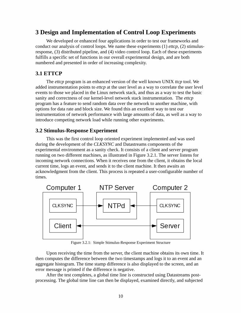
3.2 Stimulus-Response Experiment This was the first control loop oriented experiment implemented and was used
during the development of the CLKSYNC and Datastreams components of the experimental environment as a sanity check. It consists of a client and server program running on two different machines, as illustrated in Figure 3.2.1. The server listens for incoming network connections. When it receives one from the client, it obtains the local current time, logs an event, and sends it to the client machine. It then awaits an acknowledgment from the client. This process is repeated a user-configurable number of times.
Figure 3.2.1: Simple Stimulus-Response Experiment Structure
Upon receiving the time from the server, the client machine obtains its own time. It then computes the difference between the two timestamps and logs it to an event and an aggregate histogram. The time stamp difference is also displayed to the screen, and an error message is printed if the difference is negative.
After the test completes, a global time line is constructed using Datastreams post-processing. The global time line can then be displayed, examined directly, and subjected
10

to automated analysis verifying that no contradictions or constraint violations are present. Among the most important analyses on data from this experiment are those ensuring that the TSC-to-nanosecond conversion mechanism and other aspects of the global time-line construction mechanism are working properly.
3.3 Distributed Pipeline The next level of complexity for our experiments extended the stimulus-response
experiment to span an arbitrary number of machines and generalizes the data exchanged among the processing nodes. The data_pipe application runs in one of three different modes: source, sink, and processing node, with one or more data_pipe instances running on each machine in the experiment. The source node sends a small message to the first processing node in the pipeline, which forwards it on to the next node, repeating the process until the circulating message is received by the sink node, which discards it. A user-configurable number of stimuli are sent over the through the pipeline. The end-to-end response time, as well as the individual transmission intervals between each node are measured. Figure 3.3.1 illustrates a specific configuration of the Distributed Pipeline which distributes five processing nodes across four machines, with the source and sink processing nodes on the same machine.
This is important for two reasons. First, it is a functional analog of a distributed control loop as the messages proceed out across the network and then return to the sending machine. The second is that the events records for the source and sink nodes are timestamped using the same clock, since they are on the same physical machine. This fact is helpful in evaluating the precision with which the global time line can be constructed, and events on various machines can be placed on it.
Figure 3.3.1: Abstract Distributed Pipeline Configured as a Control Loop
For example, we can compare the round-trip time for a message as evaluated using
the raw send and receive timestamps produced by the common clock for the two events, and that produced by comparing the global times for the two events as mapped onto the common global time line. The experiment illustrated in Figure 3.3.1 is an abstraction of a
11

multi-machine pipeline and control loop; we run the source and sink programs on the same machine, measuring the interval between generating a message and receiving it back, as well as the intervals between sending and receiving each message at each user-level node, and at each Ethernet interface on each machine.
3.4 Video Control Loop The video control loop experiment, illustrated in Figure 3.4.1, evaluates the
performance of a video tracking application executing a simple scenario. One machine, labeled “Video Machine” in the diagram, is connected to a video camera. One KUIM thread captures video frames using the KUIM API, and then sends them through a KUIM queue to another thread executing the sending KUIM NET node, which connects though a socket to the receiving KUIM NET node on the video processing computer, labeled “Processing Machine” in the figure. Note that video frames moving through the socket connection between the two “KUIM NET” nodes is directed at the network routing level through the “NIST-NET Router” computer. This is thus one of the network connections in the experiment subject to delay simulating a connection across a network with characteristics as specified by the NIST-Net parameters specified in the NETSPEC configuration file for the experiment.
On the “Processing Machine” computer, the “KUIM Net” node receives the video frames, forwarding them through a KUIM Queue to the “Analyzer” node which tracks a specified object within the stream of video frames. The “Analyzer” node draws a box around the tracked object within each frame and sends the modified video frames through the “KUIM NET” connection to a “KUIM NET node on the ” “Display Machine”, which then sends the video frame to the X11 server process on the Display machine. This completes the data flow for the video frames from the camera on the video computer, though the tracking computation on the processing computer, and then to display on the display node.
12

Figure 3.4.1: Object Tracking Video Processing Application
On the “Processing Machine”, the KUIM “Analyzer” node also sends movement
commands to the camera based on the location of the object within the video frame to the “libptz” process. The “analyzer” thread decides when the object is close enough to an edge of the current video frame to warrant sending some combination of pan. tilt, and zoom instructions to the “Motor Control” node on the “Video Machine” to bring the tracked object closer to the center of the video frame. This is the return segment of the control loop in this experiment, which thus involves six execution threads on two machines and two network connections, both of which are subject to the network simulation delay parameters of the “NIST-Net” node, as illustrated in the diagram.
The rest of this section summarizes the duties of each thread on each machine in the video tracking experiment.
3.4.1 Video Capture Machine Threads The video capture machine is the origin and destination for the control loop, and is
labeled “Video” in Figure 3.4.1. This loop begins with the thread capturing video frames, labeled “Capture” in Figure 3.4.1, and ends with the thread listening for pan-tilt-zoom instructions which sends the corresponding commands to the camera control port, labeled “Motor Control” in Figure 3.4.1. The threads on the video capture machine, supporting video capture and camera movement are:
1. A KUIM Capture thread, which reads video frames from the camera and writes them to a shared queue
2. A KUIM Network Server thread, which reads frames from the queue and either discards them (if no client is connected on the other side of the network) or writes them into the socket connected to the corresponding KUIM Network client thread on the Processing machine
13
3. The camera movement thread, labeled “Motor Control” in Figure 3.4.1, which runs the camserv program. This program listens for pan/tilt/zoom commands from the “libptz” thread on the “processing” machine which receives information from the object tracker about object location within the frame, and which decides if camera movement is required.
In addition, there are two threads supporting the experiment infrastructure. These are the “CLKSYNC” and “DSKI” threads which support clock synchronization and Datastreams performance data gathering, respectively.
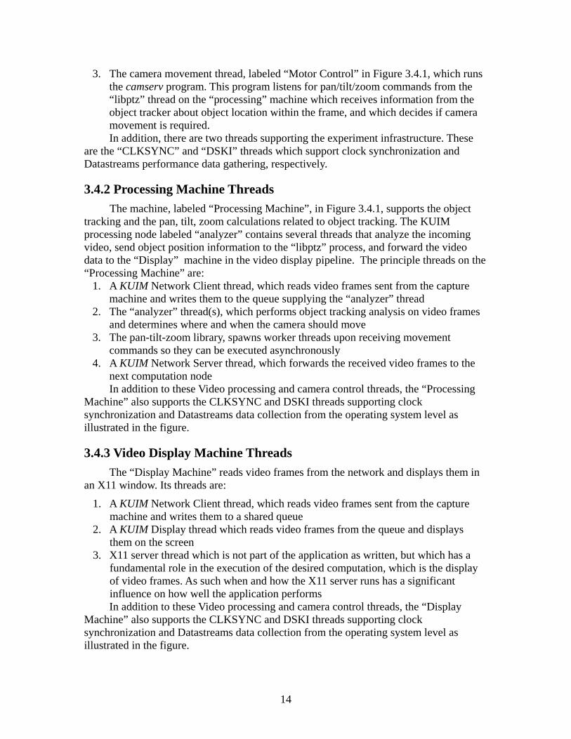
3.4.2 Processing Machine Threads The machine, labeled “Processing Machine”, in Figure 3.4.1, supports the object
tracking and the pan, tilt, zoom calculations related to object tracking. The KUIM processing node labeled “analyzer” contains several threads that analyze the incoming video, send object position information to the “libptz” process, and forward the video data to the “Display” machine in the video display pipeline. The principle threads on the “Processing Machine” are:
1. A KUIM Network Client thread, which reads video frames sent from the capture machine and writes them to the queue supplying the “analyzer” thread
2. The “analyzer” thread(s), which performs object tracking analysis on video frames and determines where and when the camera should move
3. The pan-tilt-zoom library, spawns worker threads upon receiving movement commands so they can be executed asynchronously
4. A KUIM Network Server thread, which forwards the received video frames to the next computation node
In addition to these Video processing and camera control threads, the “Processing Machine” also supports the CLKSYNC and DSKI threads supporting clock synchronization and Datastreams data collection from the operating system level as illustrated in the figure.
3.4.3 Video Display Machine Threads The “Display Machine” reads video frames from the network and displays them in
an X11 window. Its threads are:
1. A KUIM Network Client thread, which reads video frames sent from the capture machine and writes them to a shared queue
2. A KUIM Display thread which reads video frames from the queue and displays them on the screen
3. X11 server thread which is not part of the application as written, but which has a fundamental role in the execution of the desired computation, which is the display of video frames. As such when and how the X11 server runs has a significant influence on how well the application performs
In addition to these Video processing and camera control threads, the “Display Machine” also supports the CLKSYNC and DSKI threads supporting clock synchronization and Datastreams data collection from the operating system level as illustrated in the figure.
14

3.5 Performance Metrics and Experimental Parameters The first experiments we ran were designed to test the correctness of our clock
synchronization, performance data gathering, and data post-processing. We then explored the performance of control loops using the Distributed Pipeline and Object Tracking Video Processing applications on otherwise idle machines and then in the presence of competing CPU and network loads to consider the influence of competing load on control loop performance.
All the experimental scenarios were run on Pentium-class machines with two Ethernet adapters. One Ethernet adapter was connected to the LAN in our building, and only for clock synchronization messages and external SSH access. The second adapter was connected to a private LAN divided into two subnets, with a NIST-Net router between them. This network was used for the communication and data flow between the nodes in the distributed experiment.
To simulate competing network load, we ran ettcp processes in the background, sending large amounts of data between two of the nodes in the experiment. Competing CPU load was created by compiling a Linux kernel in the background on one or more of the nodes, creating a good mix of CPU and disk I/O load. The specific machines with load applied vary with different experiments, and are described in Section 4.
4 Experimental Results and Their Implications This section describes the results of the experiments described in Section 3, and
their implications for control loop performance and aspects of the system constraining the performance. Section 4.1 first describes some observations that were both significant and features of more than one experiment. Section 4.2 describes the results of the Stimulus-Response experiment, while Section 4.3 presents the results of the Distributed Pipeline experiments, and Section 4.4 describes the results of the Object tracking Video Processing experiments. Finally, Section 4.5 discusses implications of these results for control loops.
4.1 Common Issues/Observations We observed some common characteristics of our experimental results that were
notable enough to analyze in this section, before we consider each experiment individually.
4.1.3 CLKSYNC Resolution The results of some of our experiments give a good illustration of what we believe
are the measurement limits of our current methods. Figure 4.1.1 shows the Ethernet adapter to Ethernet adapter transmission time of IP datagrams, in the context of the distributed pipeline experiment. The Y-axis of this chart is at very fine resolution, with the IP datagram transmission intervals falling roughly in a 10 microsecond distribution around the median value of 40 microseconds.
15
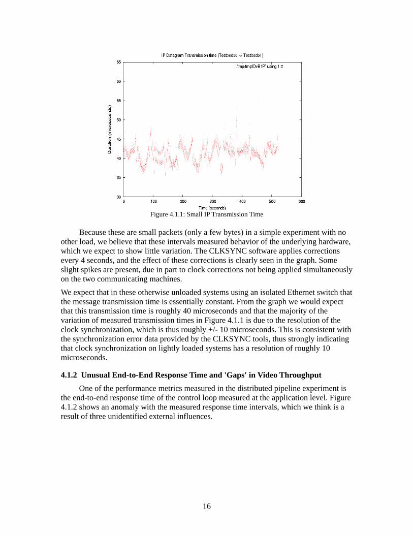
Figure 4.1.1: Small IP Transmission Time
Because these are small packets (only a few bytes) in a simple experiment with no
other load, we believe that these intervals measured behavior of the underlying hardware, which we expect to show little variation. The CLKSYNC software applies corrections every 4 seconds, and the effect of these corrections is clearly seen in the graph. Some slight spikes are present, due in part to clock corrections not being applied simultaneously on the two communicating machines.
We expect that in these otherwise unloaded systems using an isolated Ethernet switch that the message transmission time is essentially constant. From the graph we would expect that this transmission time is roughly 40 microseconds and that the majority of the variation of measured transmission times in Figure 4.1.1 is due to the resolution of the clock synchronization, which is thus roughly +/- 10 microseconds. This is consistent with the synchronization error data provided by the CLKSYNC tools, thus strongly indicating that clock synchronization on lightly loaded systems has a resolution of roughly 10 microseconds.
4.1.2 Unusual End-to-End Response Time and 'Gaps' in Video Throughput One of the performance metrics measured in the distributed pipeline experiment is the end-to-end response time of the control loop measured at the application level. Figure 4.1.2 shows an anomaly with the measured response time intervals, which we think is a result of three unidentified external influences.
16
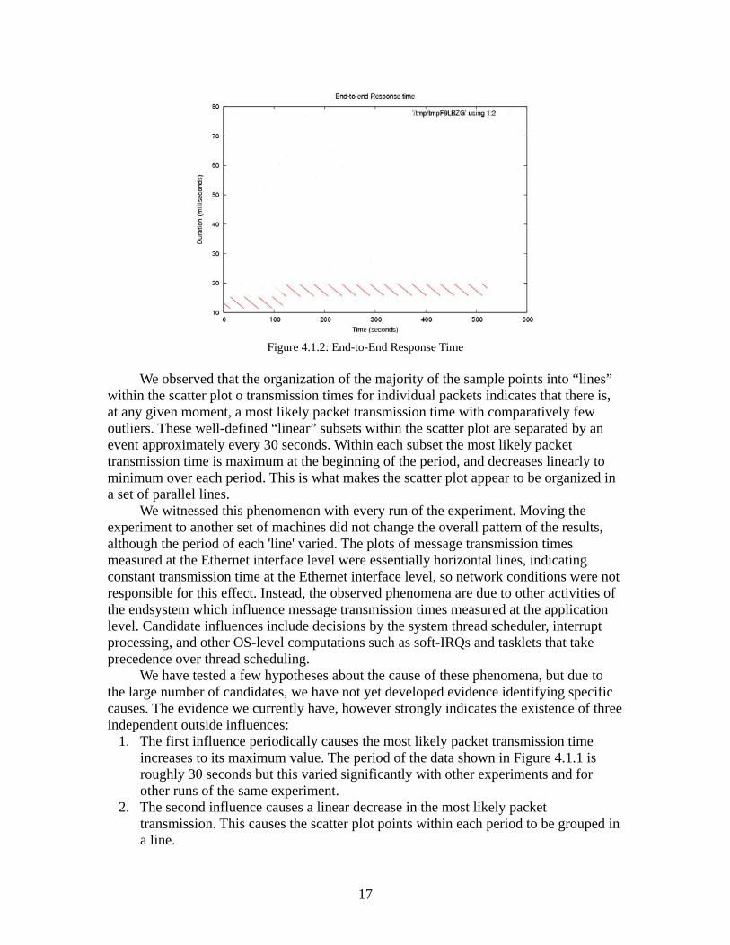
Figure 4.1.2: End-to-End Response Time
We observed that the organization of the majority of the sample points into “lines” within the scatter plot o transmission times for individual packets indicates that there is, at any given moment, a most likely packet transmission time with comparatively few outliers. These well-defined “linear” subsets within the scatter plot are separated by an event approximately every 30 seconds. Within each subset the most likely packet transmission time is maximum at the beginning of the period, and decreases linearly to minimum over each period. This is what makes the scatter plot appear to be organized in a set of parallel lines. We witnessed this phenomenon with every run of the experiment. Moving the experiment to another set of machines did not change the overall pattern of the results, although the period of each 'line' varied. The plots of message transmission times measured at the Ethernet interface level were essentially horizontal lines, indicating constant transmission time at the Ethernet interface level, so network conditions were not responsible for this effect. Instead, the observed phenomena are due to other activities of the endsystem which influence message transmission times measured at the application level. Candidate influences include decisions by the system thread scheduler, interrupt processing, and other OS-level computations such as soft-IRQs and tasklets that take precedence over thread scheduling. We have tested a few hypotheses about the cause of these phenomena, but due to the large number of candidates, we have not yet developed evidence identifying specific causes. The evidence we currently have, however strongly indicates the existence of three independent outside influences:
1. The first influence periodically causes the most likely packet transmission time increases to its maximum value. The period of the data shown in Figure 4.1.1 is roughly 30 seconds but this varied significantly with other experiments and for other runs of the same experiment.
2. The second influence causes a linear decrease in the most likely packet transmission. This causes the scatter plot points within each period to be grouped in a line.
17
3. The third outside influence appears to cause a one time change in the operating region of the most likely packet transmission time at the application level. The transition changes the operating region from ~10-15ms during the 0-100 seconds period of the experiment to ~15-20ms during the 100-500 seconds period of the experiment. At this transition point the previous maximum transmission time becomes the new minimum, and during the transition, two overlapping lines show on the scatter plot. It is important to note that this change of operating region does not appear to be instantaneous. In the graph shown, there were two most likely packet transmission time during the transition from the old operating region to the new operating region, with the transition occurring 100-120 seconds into the experiment.
While we considered the possibility that clock synchronization might be one of the causes of these phenomena, this is extremely unlikely for two reasons: (1) the start and end timestamps were taken on the same machine, and (2) the magnitude of these changes is at the millisecond level, while CLKSYNC modifications are made at the microsecond order of magnitude.
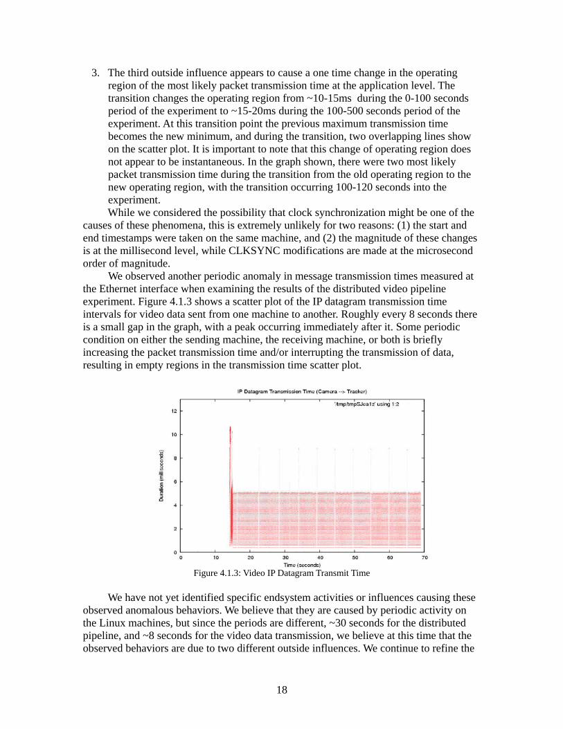
We observed another periodic anomaly in message transmission times measured at the Ethernet interface when examining the results of the distributed video pipeline experiment. Figure 4.1.3 shows a scatter plot of the IP datagram transmission time intervals for video data sent from one machine to another. Roughly every 8 seconds there is a small gap in the graph, with a peak occurring immediately after it. Some periodic condition on either the sending machine, the receiving machine, or both is briefly increasing the packet transmission time and/or interrupting the transmission of data, resulting in empty regions in the transmission time scatter plot.
Figure 4.1.3: Video IP Datagram Transmit Time
We have not yet identified specific endsystem activities or influences causing these observed anomalous behaviors. We believe that they are caused by periodic activity on the Linux machines, but since the periods are different, ~30 seconds for the distributed pipeline, and ~8 seconds for the video data transmission, we believe at this time that the observed behaviors are due to two different outside influences. We continue to refine the
18
performance data gathered and to refine our analysis in an effort to identify the source of this periodic changes in message transmission time probability, but we have not yet identified the aspects of endsystem behavior responsible because there are so many possible causes.
4.2 Stimulus-Response
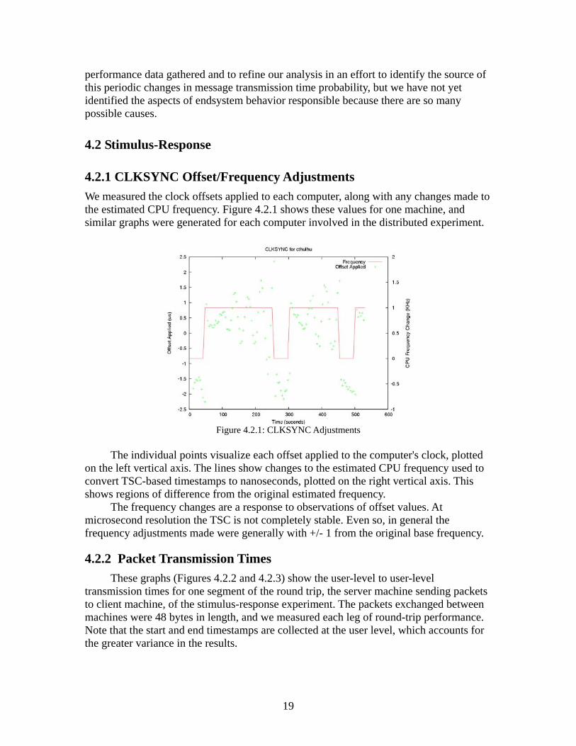
4.2.1 CLKSYNC Offset/Frequency Adjustments We measured the clock offsets applied to each computer, along with any changes made to the estimated CPU frequency. Figure 4.2.1 shows these values for one machine, and similar graphs were generated for each computer involved in the distributed experiment.
Figure 4.2.1: CLKSYNC Adjustments
The individual points visualize each offset applied to the computer's clock, plotted
on the left vertical axis. The lines show changes to the estimated CPU frequency used to convert TSC-based timestamps to nanoseconds, plotted on the right vertical axis. This shows regions of difference from the original estimated frequency.
The frequency changes are a response to observations of offset values. At microsecond resolution the TSC is not completely stable. Even so, in general the frequency adjustments made were generally with +/- 1 from the original base frequency.
4.2.2 Packet Transmission Times These graphs (Figures 4.2.2 and 4.2.3) show the user-level to user-level
transmission times for one segment of the round trip, the server machine sending packets to client machine, of the stimulus-response experiment. The packets exchanged between machines were 48 bytes in length, and we measured each leg of round-trip performance. Note that the start and end timestamps are collected at the user level, which accounts for the greater variance in the results.
19
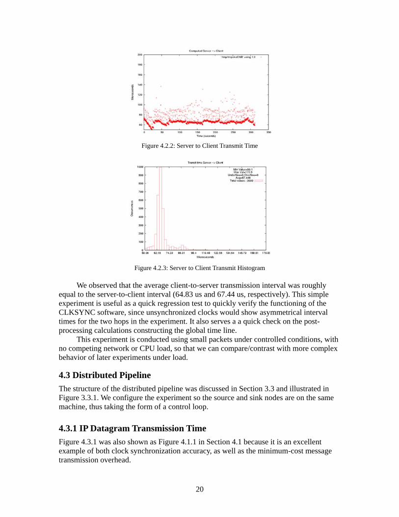
Figure 4.2.2: Server to Client Transmit Time
Figure 4.2.3: Server to Client Transmit Histogram
We observed that the average client-to-server transmission interval was roughly
equal to the server-to-client interval (64.83 us and 67.44 us, respectively). This simple experiment is useful as a quick regression test to quickly verify the functioning of the CLKSYNC software, since unsynchronized clocks would show asymmetrical interval times for the two hops in the experiment. It also serves a a quick check on the post-processing calculations constructing the global time line.
This experiment is conducted using small packets under controlled conditions, with no competing network or CPU load, so that we can compare/contrast with more complex behavior of later experiments under load.
4.3 Distributed Pipeline The structure of the distributed pipeline was discussed in Section 3.3 and illustrated in Figure 3.3.1. We configure the experiment so the source and sink nodes are on the same machine, thus taking the form of a control loop.
4.3.1 IP Datagram Transmission Time Figure 4.3.1 was also shown as Figure 4.1.1 in Section 4.1 because it is an excellent example of both clock synchronization accuracy, as well as the minimum-cost message transmission overhead.
20
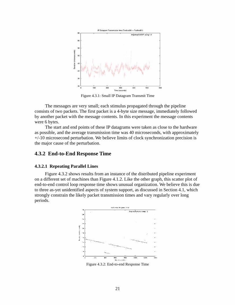
Figure 4.3.1: Small IP Datagram Transmit Time
The messages are very small; each stimulus propagated through the pipeline
consists of two packets. The first packet is a 4-byte size message, immediately followed by another packet with the message contents. In this experiment the message contents were 6 bytes.
The start and end points of these IP datagrams were taken as close to the hardware as possible, and the average transmission time was 40 microseconds, with approximately +/-10 microsecond perturbation. We believe limits of clock synchronization precision is the major cause of the perturbation.
4.3.2 End-to-End Response Time
4.3.2.1 Repeating Parallel Lines Figure 4.3.2 shows results from an instance of the distributed pipeline experiment on a different set of machines than Figure 4.1.2. Like the other graph, this scatter plot of end-to-end control loop response time shows unusual organization. We believe this is due to three as-yet unidentified aspects of system support, as discussed in Section 4.1, which strongly constrain the likely packet transmission times and vary regularly over long periods.
Figure 4.3.2: End-to-end Response Time
21

4.3.2.2 Competing CPU Load
We introduced competing CPU/IO load into the experiment by running a Linux kernel compile on the source/sink machine in the distributed pipeline. The disk interrupt processing load of this activity is just as important as the competition for CPU cycles.
One important effect of the competing load is a reduced accuracy of clock synchronization. As shown in Figure 4.3.3, the offsets applied to the clock were larger than in the unloaded scenario, increasing the estimated clock error from 10 microseconds to about 20. There were also more frequent adjustments to the CPU frequency, within range of +/-2 of the starting frequency.
Figure 4.3.3: CLKSYNC Adjustments Made
In future work, we would like to place some or all of the clock synchronization
software under explicit scheduler control to strongly isolate it from the competing load, which should make the clock synchronization accuracy much more independent of system CPU load. In addition, although we have tried to place the NTP time stamp collection as close to the hardware as possible, it appears that CPU scheduling may still play a role in the accuracy of clock synchronization we are able to obtain.
Figure 4.3.4: IP Datagram Transmission
The overall results were similar to the unloaded scenario, with the same unusual
organization in the end-to-end control loop scatter plot. The only significant difference we observed was that the average packet transmission times to and from the loaded machine increased from 40us to 70us.
22

4.3.2.3 Competing Network Load
For a competing network load scenario, we ran ettcp processes dumping large amounts of data between the third and fourth machines in the control loop. Unlike the competing CPU load scenario, clock synchronization was unaffected for the loaded machines.
The effects on the end-to-end results were striking, with the average response time at 275ms, with a large variance around the average value (Figures 4.3.5 and 4.3.6). In addition, we observed a different pattern of unusual organization in the scatter plot. The end-to-end response time periods appear to be roughly quantized at 5ms intervals. This is an interesting effect, and we will continue to refine our instrumentation and analysis to determine its origins.
Figure 4.3.5: End-to-end Response Time
Figure 4.3.6: End-to-end Response Time
Examination of the individual node-to-node IP datagram transmission intervals showed that each leg of the trip through the pipeline had fairly consistent results, with a greater number of outliers to and from the machines under competing load being unsurprising. However, no quantization of the scale observed in the end-to-end data was
23

noted in the individual transmission intervals, which simply measure the networking hardware performance. This indicates that the quantization is associated with endsystem processing of the network flows, rather than effects of the network itself. That is also not surprising as the network in this case was a simple Ethernet switch.
Therefore, we believe that the quantization is due to OS and user-level computation scheduling and is not a function of network performance. Future work will vary the amount of competing load so that we can discover how control loop performance varies with competing network load.
4.4 Distributed Video Tracking The design of the object tracking video processing control loop experiment was discussed in Section 3.4 and illustrated in Figure 3.4.1. The video frames flow from the camera to a tracking process which forwards modified frames to the display computer, and send camera movement commands back to the camera machine.
4.4.1 IP Data Transmission Time The first set of measurements taken show the transmission of the IP datagrams
carrying the captured video across the network. Of particular interest was the video data transmission intervals for frames sent from the capture machine to the tracker, which had the NIST-Net box between them to simulate network conditions creating larger packet delays than that of the local Ethernet switches used in other experiments.
4.4.1.1 Initial Warm-Up Period of More Chaotic Behavior We noticed that in all runs of the distributed pipeline experiment that there was a
period of chaotic activity at the beginning, which stabilized to more consistent behavior after a brief period. Figures 4.4.1 and 4.4.2 show two 60-second experiments; the former with no NIST-Net delay applied, and the latter with a 200ms delay.
Figure 4.4.1: No NIST-Net Delay
24
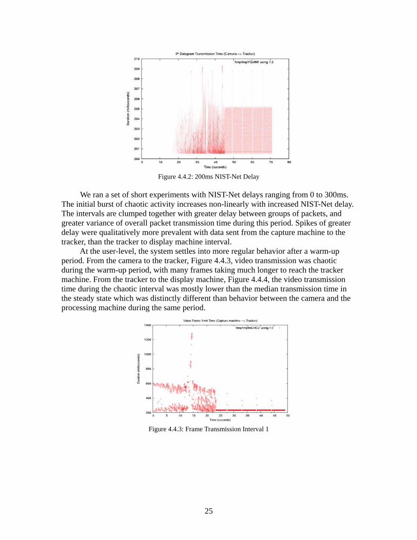
Figure 4.4.2: 200ms NIST-Net Delay
We ran a set of short experiments with NIST-Net delays ranging from 0 to 300ms.
The initial burst of chaotic activity increases non-linearly with increased NIST-Net delay. The intervals are clumped together with greater delay between groups of packets, and greater variance of overall packet transmission time during this period. Spikes of greater delay were qualitatively more prevalent with data sent from the capture machine to the tracker, than the tracker to display machine interval.
At the user-level, the system settles into more regular behavior after a warm-up period. From the camera to the tracker, Figure 4.4.3, video transmission was chaotic during the warm-up period, with many frames taking much longer to reach the tracker machine. From the tracker to the display machine, Figure 4.4.4, the video transmission time during the chaotic interval was mostly lower than the median transmission time in the steady state which was distinctly different than behavior between the camera and the processing machine during the same period.
Figure 4.4.3: Frame Transmission Interval 1
25
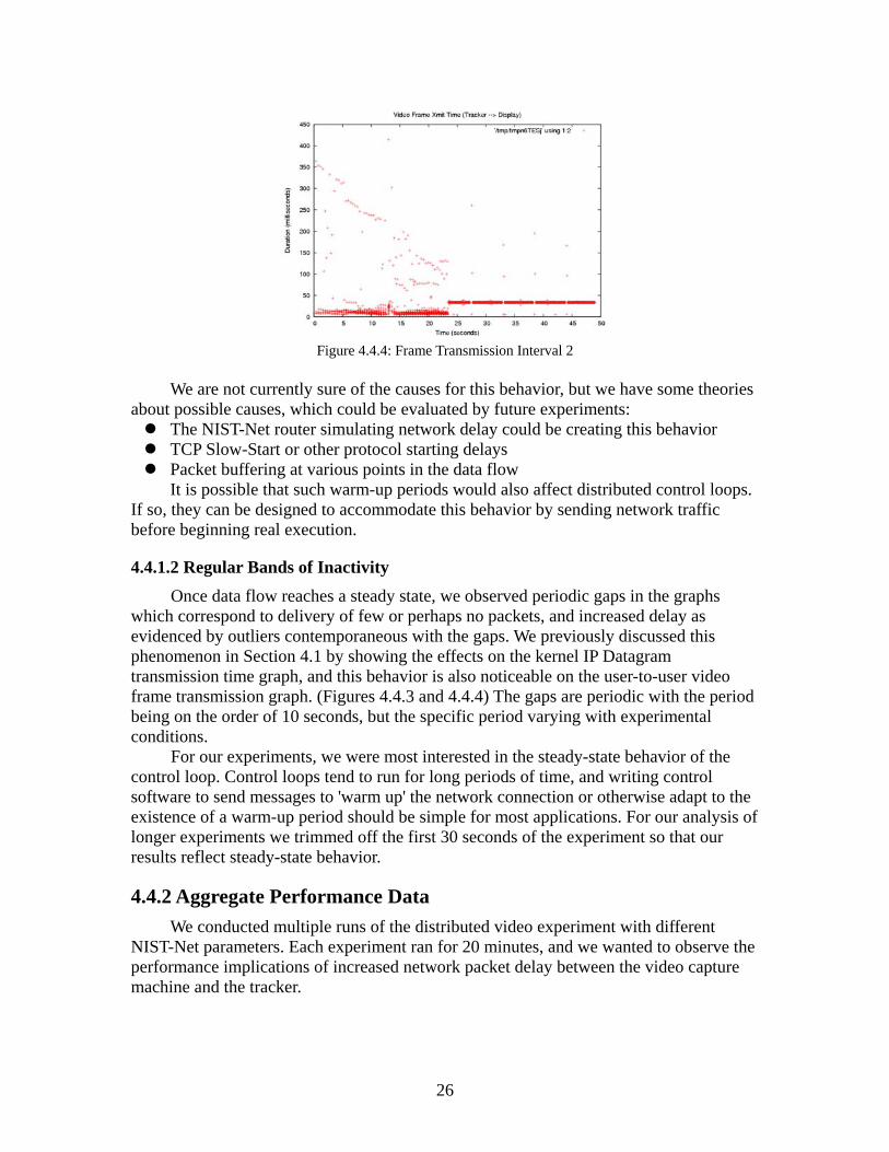
Figure 4.4.4: Frame Transmission Interval 2
We are not currently sure of the causes for this behavior, but we have some theories
about possible causes, which could be evaluated by future experiments: The NIST-Net router simulating network delay could be creating this behavior TCP Slow-Start or other protocol starting delays Packet buffering at various points in the data flow
It is possible that such warm-up periods would also affect distributed control loops. If so, they can be designed to accommodate this behavior by sending network traffic before beginning real execution.
4.4.1.2 Regular Bands of Inactivity
Once data flow reaches a steady state, we observed periodic gaps in the graphs which correspond to delivery of few or perhaps no packets, and increased delay as evidenced by outliers contemporaneous with the gaps. We previously discussed this phenomenon in Section 4.1 by showing the effects on the kernel IP Datagram transmission time graph, and this behavior is also noticeable on the user-to-user video frame transmission graph. (Figures 4.4.3 and 4.4.4) The gaps are periodic with the period being on the order of 10 seconds, but the specific period varying with experimental conditions.
For our experiments, we were most interested in the steady-state behavior of the control loop. Control loops tend to run for long periods of time, and writing control software to send messages to 'warm up' the network connection or otherwise adapt to the existence of a warm-up period should be simple for most applications. For our analysis of longer experiments we trimmed off the first 30 seconds of the experiment so that our results reflect steady-state behavior.
4.4.2 Aggregate Performance Data We conducted multiple runs of the distributed video experiment with different NIST-Net parameters. Each experiment ran for 20 minutes, and we wanted to observe the performance implications of increased network packet delay between the video capture machine and the tracker.
26

4.4.2.1 Aggregate IP-Level Delay
Figure 4.4.5 shows the mean and standard deviation of the IP datagrams sent from the capture machine to the tracker, as a function of NIST-Net delay. Regardless of the NIST-Net parameters set, the variance of hardware-to-hardware delay remained the same, and was relatively small (~ 5ms) as expected, since the measurement points were not not subject to endsystem interaction effects. The average delay was a linear function of the NIST-Net delay setting.
Figure 4.4.5: Aggregate IP-Level Delay
4.4.2.2 Aggregate User-Level Video Frame delay The results for the user-level video frame transmission intervals, Figure 4.4.6, were similar. The average delay was a linear function of NIST-Net delay setting, with a higher magnitude than the IP level graph, due to influence of added overhead of the network stack, application thread scheduling, and any other endsystem interactions. The variance was relatively uniform but significantly larger than the kernel level interval data. This follows from three main sources: (1) packet fragmentation and reassembly since the variance of the frame will reflect the combined effects for each packet into which the video frame is decomposed, (2) hardware interrupt, soft-IRQ, and application thread scheduling delays, and (3) the smaller number of sample points, since any given video frame is decomposed into ~50 individual IP datagrams.
27
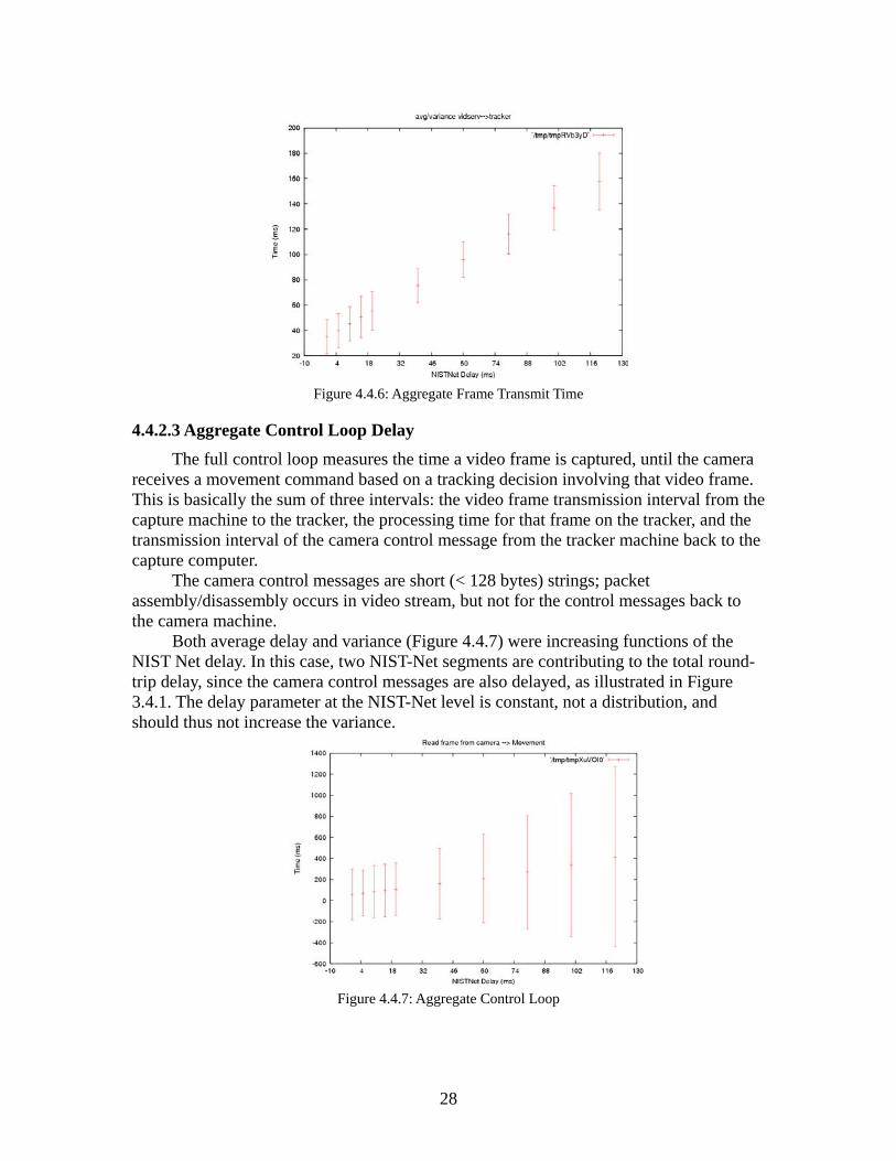
Figure 4.4.6: Aggregate Frame Transmit Time
4.4.2.3 Aggregate Control Loop Delay The full control loop measures the time a video frame is captured, until the camera
receives a movement command based on a tracking decision involving that video frame. This is basically the sum of three intervals: the video frame transmission interval from the capture machine to the tracker, the processing time for that frame on the tracker, and the transmission interval of the camera control message from the tracker machine back to the capture computer.
The camera control messages are short (< 128 bytes) strings; packet assembly/disassembly occurs in video stream, but not for the control messages back to the camera machine.
Both average delay and variance (Figure 4.4.7) were increasing functions of the NIST Net delay. In this case, two NIST-Net segments are contributing to the total round-trip delay, since the camera control messages are also delayed, as illustrated in Figure 3.4.1. The delay parameter at the NIST-Net level is constant, not a distribution, and should thus not increase the variance.
Figure 4.4.7: Aggregate Control Loop
28

However, the increase of the variance is clearly super-linear, and the shape of the curve suggests a quadratic function of delay rather than linear.
4.4.3 Competing Loads More interesting than the unloaded scenario is the performance of the control loop
when competing network and CPU loads are applied to various stages of the control loop. Like the distributed pipeline experiment, we used background kernel compiles and ettcp to create conditions including competing CPU load, disk I/O interrupt processing and network traffic.
4.4.3.1 Competing CPU/Disk Load We created a mix of CPU and I/O load by compiling a Linux Kernel in the
background on the video capture machine. Our first observation was that, similar to our other experiments, the accuracy of our clock synchronization was degraded. Although the CLKSYNC messages were transmitted on a separate network from the experimental network traffic, we believe that interrupt and soft-IRQ packet processing on reception caused greater uncertainty in the clock correction offsets. In this case, the offsets applied ranged from -15 to +20 microseconds (Figure 4.4.8), rather than +/- 10 microseconds for the unloaded experiments.
Figure 4.4.8: Clock Synchronization
However, despite the degradation in clock synchronization, the overall results of the
experiment were about the same. We have a few theories about why this is the case:
Disk I/O interrupts are of lower priority than network interrupts on the Linux kernel with the RT-Patch we are using, which would mean that network processing is isolated from the competing disk load
Since the kernel compile is a mix of CPU and disk operations, the video capture program CPU use can apparently fit into gaps left without noticeably degrading video performance
The main line Linux scheduler attempts to classify processes on its own according to their pattern of computational activity into interactive and batch classes, with interactive processes given preference. It is possible, though not verified, that the video processing CPU use pattern is classified as interactive and thus given precedence over the kernel compilation.
29
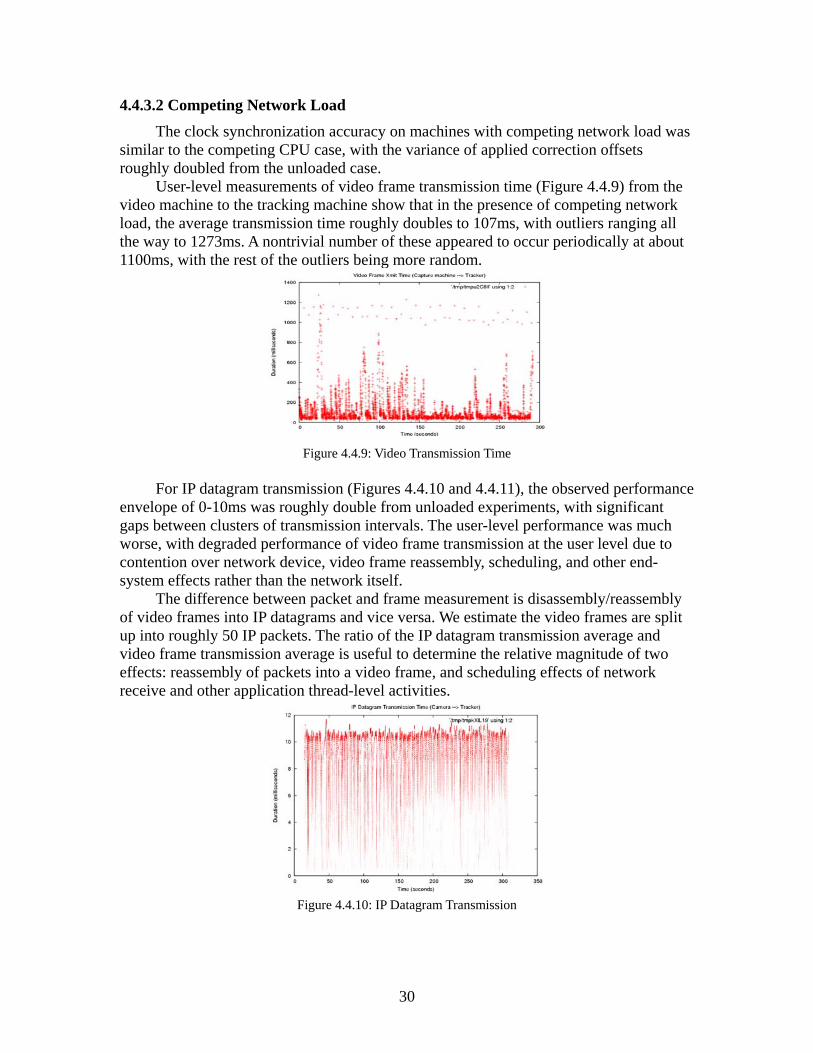
4.4.3.2 Competing Network Load
The clock synchronization accuracy on machines with competing network load was similar to the competing CPU case, with the variance of applied correction offsets roughly doubled from the unloaded case. User-level measurements of video frame transmission time (Figure 4.4.9) from the video machine to the tracking machine show that in the presence of competing network load, the average transmission time roughly doubles to 107ms, with outliers ranging all the way to 1273ms. A nontrivial number of these appeared to occur periodically at about 1100ms, with the rest of the outliers being more random.
Figure 4.4.9: Video Transmission Time
For IP datagram transmission (Figures 4.4.10 and 4.4.11), the observed performance envelope of 0-10ms was roughly double from unloaded experiments, with significant gaps between clusters of transmission intervals. The user-level performance was much worse, with degraded performance of video frame transmission at the user level due to contention over network device, video frame reassembly, scheduling, and other end-system effects rather than the network itself. The difference between packet and frame measurement is disassembly/reassembly of video frames into IP datagrams and vice versa. We estimate the video frames are split up into roughly 50 IP packets. The ratio of the IP datagram transmission average and video frame transmission average is useful to determine the relative magnitude of two effects: reassembly of packets into a video frame, and scheduling effects of network receive and other application thread-level activities.
Figure 4.4.10: IP Datagram Transmission
30
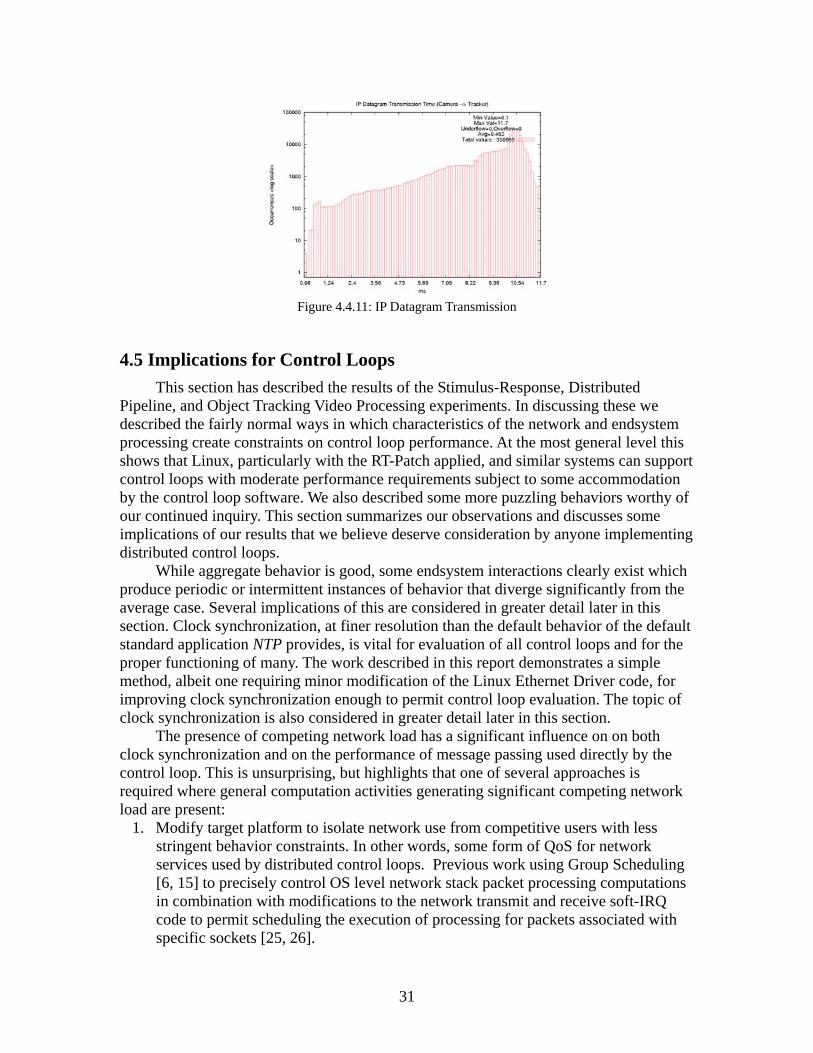
Figure 4.4.11: IP Datagram Transmission
4.5 Implications for Control Loops This section has described the results of the Stimulus-Response, Distributed Pipeline, and Object Tracking Video Processing experiments. In discussing these we described the fairly normal ways in which characteristics of the network and endsystem processing create constraints on control loop performance. At the most general level this shows that Linux, particularly with the RT-Patch applied, and similar systems can support control loops with moderate performance requirements subject to some accommodation by the control loop software. We also described some more puzzling behaviors worthy of our continued inquiry. This section summarizes our observations and discusses some implications of our results that we believe deserve consideration by anyone implementing distributed control loops. While aggregate behavior is good, some endsystem interactions clearly exist which produce periodic or intermittent instances of behavior that diverge significantly from the average case. Several implications of this are considered in greater detail later in this section. Clock synchronization, at finer resolution than the default behavior of the default standard application NTP provides, is vital for evaluation of all control loops and for the proper functioning of many. The work described in this report demonstrates a simple method, albeit one requiring minor modification of the Linux Ethernet Driver code, for improving clock synchronization enough to permit control loop evaluation. The topic of clock synchronization is also considered in greater detail later in this section. The presence of competing network load has a significant influence on on both clock synchronization and on the performance of message passing used directly by the control loop. This is unsurprising, but highlights that one of several approaches is required where general computation activities generating significant competing network load are present:
1. Modify target platform to isolate network use from competitive users with less stringent behavior constraints. In other words, some form of QoS for network services used by distributed control loops. Previous work using Group Scheduling [6, 15] to precisely control OS level network stack packet processing computations in combination with modifications to the network transmit and receive soft-IRQ code to permit scheduling the execution of processing for packets associated with specific sockets [25, 26].
31
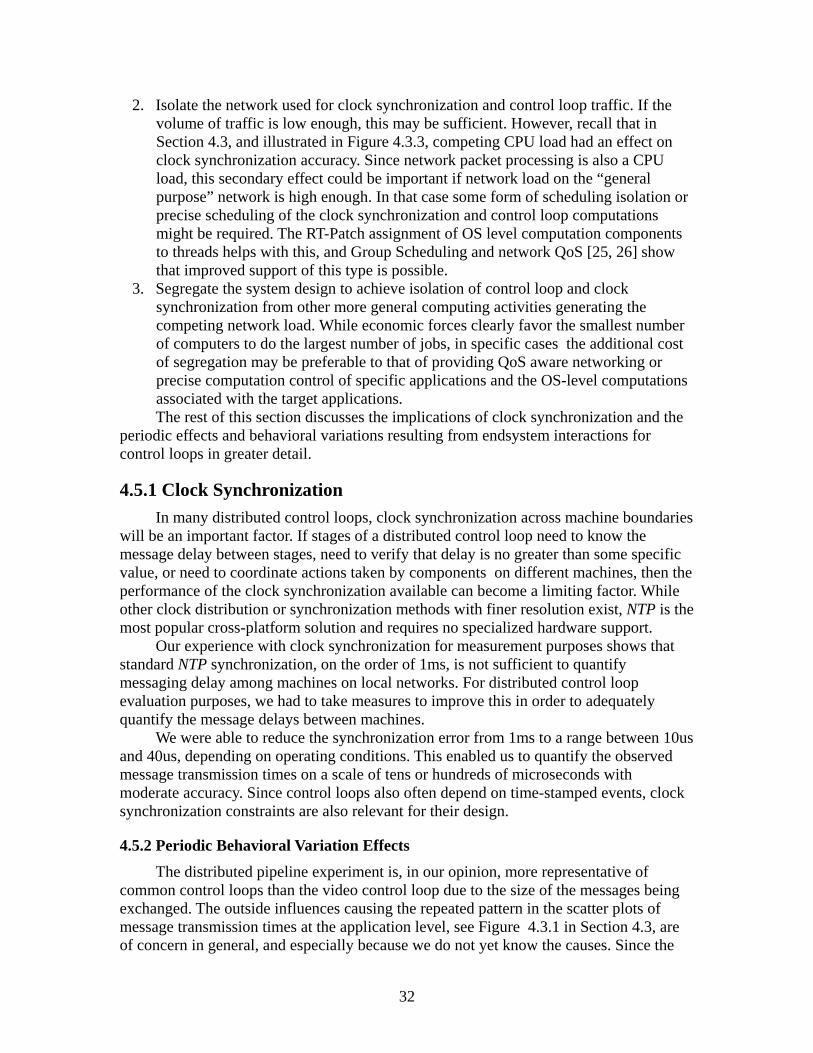
2. Isolate the network used for clock synchronization and control loop traffic. If the volume of traffic is low enough, this may be sufficient. However, recall that in Section 4.3, and illustrated in Figure 4.3.3, competing CPU load had an effect on clock synchronization accuracy. Since network packet processing is also a CPU load, this secondary effect could be important if network load on the “general purpose” network is high enough. In that case some form of scheduling isolation or precise scheduling of the clock synchronization and control loop computations might be required. The RT-Patch assignment of OS level computation components to threads helps with this, and Group Scheduling and network QoS [25, 26] show that improved support of this type is possible.
3. Segregate the system design to achieve isolation of control loop and clock synchronization from other more general computing activities generating the competing network load. While economic forces clearly favor the smallest number of computers to do the largest number of jobs, in specific cases the additional cost of segregation may be preferable to that of providing QoS aware networking or precise computation control of specific applications and the OS-level computations associated with the target applications.
The rest of this section discusses the implications of clock synchronization and the periodic effects and behavioral variations resulting from endsystem interactions for control loops in greater detail.
4.5.1 Clock Synchronization In many distributed control loops, clock synchronization across machine boundaries will be an important factor. If stages of a distributed control loop need to know the message delay between stages, need to verify that delay is no greater than some specific value, or need to coordinate actions taken by components on different machines, then the performance of the clock synchronization available can become a limiting factor. While other clock distribution or synchronization methods with finer resolution exist, NTP is the most popular cross-platform solution and requires no specialized hardware support. Our experience with clock synchronization for measurement purposes shows that standard NTP synchronization, on the order of 1ms, is not sufficient to quantify messaging delay among machines on local networks. For distributed control loop evaluation purposes, we had to take measures to improve this in order to adequately quantify the message delays between machines. We were able to reduce the synchronization error from 1ms to a range between 10us and 40us, depending on operating conditions. This enabled us to quantify the observed message transmission times on a scale of tens or hundreds of microseconds with moderate accuracy. Since control loops also often depend on time-stamped events, clock synchronization constraints are also relevant for their design.
4.5.2 Periodic Behavioral Variation Effects
The distributed pipeline experiment is, in our opinion, more representative of common control loops than the video control loop due to the size of the messages being exchanged. The outside influences causing the repeated pattern in the scatter plots of message transmission times at the application level, see Figure 4.3.1 in Section 4.3, are of concern in general, and especially because we do not yet know the causes. Since the
32
magnitude of the changes in behavior is fairly small, about 5ms, there will be many distributed control loops for which this variation is below thresholds of concern. However, identifying and eliminating these sources of behavioral changes would clearly permit distributed control loops with more stringent behavioral constraints to also be supported. It is important to note that all of these experiments use only the main line Linux scheduling methods with minor RT-Patch modifications to specify the control loop behavior. Other, more precise scheduling methods exist, and could reduce some of the observed periodic effects on packet transmission time. However, exploring these would be outside the scope of this study which concentrated on factors affecting control loop performance in standard Linux. We did use the RT-Linux patch, which is arguably not standard, but we considered it the most likely target for Linux-based control loop software. The warm-up period observed in the distributed video experiment, if not solely an artifact of using the NIST-Net delay router, is clearly a factor which the control software would have to handle. However, this should be easy to do for many applications. More problematic are the periodic delays observed in the video pipeline experiment, because this represents a constraining factor on the dependable message delivery time constraints of the control loop. The worst-case response time of the control loop would either have to include the occurrence of these higher-magnitude delays, or the control loop would have to permit using a synthesized value, perhaps averaged or projected from the previous N sample points. As long as these intermittent periods of aberrant behavior did too many sample periods, many control algorithms would be perfectly happy. However, it would clearly be better if such periods of different behavior did not exist, because the control loop computations could be simpler and the worst-case period of the control loop would be smaller. The evidence indicates that the major, if not sole, causes of these periodic changes in behavior are interaction of the control loop computations with other endsystem activities. We continue to refine our experiments and instrumentation to investigate our hypotheses about these activities and we hope to be able to control or eliminate their interference. Future experiments extending this work would include attempting to use the Linux RT priority scheduling class to improve performance of control loops. More specialized control approaches, such as Group Scheduling [6,15] permit control of both user-level control loop threads and associated OS-level Hard-IRQ and Soft-IRQ network processing threads. Whether such specialized and precise methods will be relevant depend on the nature of the sources for the periodic behavior variation.
5 Conclusions and Future Work This document has presented the work we have done in developing a system
framework for evaluating the performance of distributed control loops. One of the most significant challenges in making this evaluation possible was the need to improve the resolution of clock synchronization provided by generic NTP by a factor of roughly 40 to make the evaluation of distributed control loops possible. The clock values on various machines were then used to timestamp event records gathered using the Datastreams instrumentation methods, and post-processing analysis of several kinds was described
33
which placed endsystem events on a global time line, and which were then used to evaluate the performance of specific distributed control loops in several ways. We created methods for automatically and reproducibly executing distributed computations used as example control loop applications. These and other supporting methods and tools were discussed in Section 2. Section 3 discussed the experiment design and implementation including the Stimulus-Response, Distributed Pipeline, and Object tracking Video Processing application computations.
Section 4 discussed the results of our experiment, which revealed a number of interesting factors constraining the performance of distributed control loops and having important implications for their implementation. The results revealed that Linux with the RT-Patch is an excellent target platform for distributed control loop applications with moderate computation behavior constraints, but that there are some endsystem interactions of interest. These endsystem interactions constrain the performance of the distributed control loop applications and produce periodic behavioral variation effects which could be handled by some distributed control loop applications, but which would have to be eliminated for others to use th target platform. However, it is also likely that previously investigated methods for precise computation control and for integrated scheduling of application-level computations with the OS-level computation components supporting them could eliminate many or all of these periodic behavioral variations. Other methods of isolation and control are possible, and all are applicable to other platforms than Linux, although Linux with the RT-Patch is an increasingly popular target platform for distributed control loop and other applications requiring some form of real-time or other precise computation control support.
As with any project involving development and experimentation, there are a number of interesting topics for future work. The Datastreams framework for gathering and analyzing performance data is at a highly evolved and stable state. It provides excellent support for performance evaluation of application-level, OS-level, and distributed application behavior. Future work in this area will involve increasingly sophisticated used of run-time filters to decrease instrumentation overhead, increase run-time use of performance data and increase the dynamic adaptability of the performance data gathering. In the post-processing area we steadily increase the set of available filters and analyses, and for some types of analysis generalized support for distributing data analysis pipelines across several machines would be desirable. Other tools, such as CLKSYNC and the latest implementation of NETSPEC are at earlier stages of development and would benefit from more basic improvements. Such desirable improvements in the current set of tools and methods include: • Modify the CLKSYNC tools to use their own communication protocol,
rather than as a modification of NTP. • Add Datastreams instrumentation to the NIST Net package, in order to
distinguish real network delays from OS-level scheduling on the router machine.
• Further refine the NETSPEC communication protocol, and improve both the error handling and the user interface of the ns_control application.
• Devise an instrumentation and analysis method capable of associating individual IP datagrams with their respective video frames in the video
34
object tracking experiment. • Use Group Scheduling on the endsystem to see if integrated and
precise control of the experimental applications' user and OS level components would improved performance. Similarly, it would be good to see if such precise control could be used to increase the isolation of control loop component performance from the disruptive influence of other endsystem activities.
• Introduce a distributed version of the Group Scheduling framework, and investigate whether fine-grained scheduling control across machine boundaries will improve performance beyond improvements provided by integrating control of user and OS computation components within and endsystem.
• Expand the video pipeline experiment to include additional cameras, more sophisticated tracking, and additional computation nodes. The work described here demonstrated that distributed control loop type
computations could be implemented and their behavior evaluated in detail. The methods and tools demonstrated, extended and in some cases developed provide an effective platform for a wide variety of related distributed application development and evaluation. We intend to continue some of the work described here and to use and extend the methods and tools discussed in this report in support of other projects in the future.
35

6 References [1] D. P. Bovet and M. Cesati. Understanding the Linux Kernel. O'Reilly and Associates,
Inc., 3rd edition, 2005. [2] C. Benvenuti. Understanding Linux Network Internals. O'Reilly and Associates, Inc.,
2005. [3] J. Corbet, A. Rubini, and G. Kroah-Hartman. Linux Device Drivers. O'Reilly and
Associates, Inc., 3rd edition, 2005. [4] B. Buchanan, D. Niehaus, G. Dhandapani, R. Menon, S. Sheth, Y.Wijata, and S.
House. The Datastream Kernel Interface (Revision A). Technical Report ITTC-FY98-TR-11510-04, Information and Telecommunication Technology Center, University of Kansas, 1994 June.
[5] M. Carson and D. Santay. NIST Net – A Linux-based Network Emulation Tool. Computer Communication Review, 2003. http://www-x.antd.nist.gov/nistnet/nistnet.pdf
[6] T. Aswathanarayana, V. Subramonian, D. Niehaus, and C Gill. Design and Performance of Configurable Endsystem Scheduling Mechanisms. IEEE Real-Time and Embedded Technology and Applications Symposium, March 2005.
[7] ETTCP. http://sourceforge.net/projects/ettcp/. [8] H. Subramanian. Systems Performance Evaluation Methods for Distributed Systems
Using Datastreams. Master’s thesis, University of Kansas, 2005. [9] L. Torvalds et al. The Linux Kernel Archives. http://www.kernel.org/[10] D. L. Mills. On the Accuracy and Stability of Clocks Synchronized by the Network
Time Protocol in the Internet System. Computer Communication Review, 20(1):65-75, 1990.
[11] R. Jonkman, D. Niehaus, J. Evans, and V. Frost. NetSpec: A Network Performance Evaluation Tool. Technical Report ITTC-FY98-TR-10980-28, Information and Telecommunication Technology Center, University of Kansas, December 1998.
[12] S. Rostedt and D. Hart. Internals of the RT Patch. Proceedings of the Linux Symposium, 161-172, June 2007.
[13] Slashdot.org Article, “Playing Music Slows Vista Network Performance?”, http://it.slashdot.org/article.pl?sid=07/08/21/1441240, August 21, 2007
[14] M. Russinovich, “Vista Multimedia Playback and Network Throughput”, http://blogs.technet.com/markrussinovich/archive/2007/08/27/1833290.aspx, August, 27, 2007.
[15] M. Frisbie, D. Niehaus, V. Subramonian, and C. Gill, “Group Scheduling in System Software,” Workshop on Parallel and Distributed Real-Time Systems, in Proceedings of IPDPS 2004, Santa Fe, NM, April 2004.
[16] T. Gleixner and D. Niehaus, "Hrtimers and Beyond: Transforming the Linux Time Subsystems",Proceedings of the Ottawa Linux Symposium, Ottawa, Ontario, Canada, July 2006.
[17]D. Niehaus, “KURT-Linux Support for Adaptive Computing”, 11th International Workshop on Parallel and Distributed Real-Time Systems, in Proceedings of IPDPS 2003, Nice France, April 2003.
[18] S. B. House, D. Niehaus, “Synchronous Fine-Grain Distributed Computations,” Proceedings of the Real-Time Technology and Applications Symposium, Washington
36

D.C., June 2000. [19] B. Srinivasan, S. Pather, R. Hill, F. Ansari, D. Niehaus. “A Firm Real-Time System
Implementation Using Commercial Off-The Shelf Hardware and Free Software”, Proceedings of the Real-Time Technology and Applications Symposium, Denver, June 1998
[20] P. Prasithsangaree, D. Niehaus, "Multiple QoS Routing in Large PNNI ATM Networks with Heavy Traffic," The 2002 International Symposium on Performance Evaluation of Computer and Telecommunication Systems (SPECTS'02), San Diego, California, July 14-18, 2002, pp. 438-442.
[21] K. Yaghmour and M. Dagenais, “Measuring and Characterizing System Behavior Using Kernel-Level Event Logging”, USENIX Annual Technical Conference, 2000.
[22] Y. Wijata and D. Niehaus and V. Frost, “A Scalable Agent-based Network Measurement Infrastructure”, IEEE Communications, 38(9), September, 2000, pp.174—183.
[23] RT-Linux, FSM Labs, http://www.fsmlabs.com[24] Timesys, http://www.timesys.com[25] H. Sampathkumar, “Using Time Division Multiplexing to Support Real-time
Networking on Ethernet”, Master's Thesis, EECS Department, University of Kansas 2004.
[26] B. Subramanyan, “Real-Time Networking for Quality of Service on TDM Based Ethernet”, Master's Thesis, EECS Department, University of Kansas, 2004.
37
7 Appendices Appendices A, B, and C provide a modest amount of additional and more detailed
information about the Datastreams, CLKSYNC, and NETSPEC methods and tools. The information in the appendices was at a finer level of detail than was appropriate for the main sections of the report, but are provided because it may be of interest to readers who wish to learn a little more about the implementation details of components of the experiments discussed in this report.
A. Datastreams Datastreams is a Linux kernel patch, user-level library, and set of related tools for
collecting and analyzing performance data. Developers place instrumentation point macros within the kernel or user-level applications, and during execution a binary file containing the instrumentation data is written to the disk. The data within this binary file can be further analyzed, filtered, and transformed using the post-processing software.
A.1 Entity Types When an instrumentation point is encountered, the performance data written to the
output file is called an entity. There are four different types of entities, outlined below. In addition, the macro definitions of some of the more commonly used instrumentation are shown.
A.1.1 Events Events are the simplest entity type, which indicates that some named event occurred
at a specific time. All events may have a long integer tag value saved with it, and optionally a sized chunk of extra data.
DSTRM_EVENT(<group name>, <entity name>, <tag_value>) DSTRM_EVENT_DATA(<group name>, <entity name>, <tag value>, <size>, <data pointer>, <decoder function name>)
A.1.2 Intervals Intervals represent an elapsed time, with macros for start and end points. The start
point notes the time it was called, and the end point logs the elapsed time to the data stream. As with events, intervals can be tagged with an integer value.
DSTRM_INTERVAL_START(<group name>, <entity name>) DSTRM_INTERVAL_END(<group name>, <entity name>, <tag value)
A.1.3 Counters Maintains a value that is incremented each time the counter's instrumentation point
is executed. The counter total can be logged at any time, and it can be reset to zero. Counters have significantly less logging overhead than events.
DSTRM_COUNTER_ADD(<group name>, <entity name>, <amount>) DSTRM_COUNTER_LOG(<group name>, <entity name>) DSTRM_COUNTER_RESET(<group name>, <entity name>)
38
A.1.4 Histograms
Histograms keep a data structure that can be used to generate a graphical display of tabulated frequencies. The histogram is parameterized with a range and a number of 'buckets' representing intervals of input data. Histogram instrumentation points increment the appropriate bucket based on the given value, and can be logged to the data stream or reset at any time. Histograms can also be constructed in post-processing from other entity types, and can be sent to GNUPlot to be rendered graphically.
DSTRM_HISTOGRAM_ADD(<group name>, <entity name>, <amount>) DSTRM_HISTOGRAM_LOG(<group name>, <entity name>) DSTRM_HISTOGRAM_RESET(<group name>, <entity name>)
A.2 Entity Namespace All the entities within an application have metadata associated with them. There is a
two-level hierarchy of names--group name and entity name. This allows for performing operations on groups of entities, which is convenient for enabling/disabling them at runtime, and also for various levels of analysis during post-processing. Entities also may have a description as well as entity-specific metadata. For example, events that log extra data will give a string that names a Python function that can unpack the binary extra data during post-processing.
For performance reasons, it is inefficient to log these strings every time an instrumentation point is encountered. Instead, at the beginning of any output file a set of namespace data is produced, which declares the names of all the instrumentation points within the application, their metadata, and a unique id. Subsequent entities are logged only by this id, making the entity data structure very small, reducing instrumentation overhead.
Both DSKI and DSUI use special binary text sections, GCC attributes, and linker operations to automatically extract the namespace information from the compiled application itself. Other languages may not support this; in this case special namespace files must be created.
A.3 Data Stream Management By default, no entities are logged in the kernel or application when it is running. To
log data, a data stream must be created. A data stream is associated with a set of buffers, an output file to write data to, and some other parameters. Any data stream has a set of entities associated with it. Initially this set is empty; the user can ‘turn on’ entities for that data stream through configuration options. Any time an instrumentation point is encountered during execution, the corresponding entity is logged to all data streams that have that entity enabled.
Two fundamental data stream types are implemented: normal and ring buffer. Normal data streams send entities to the output file as they receive them. Ring buffer data streams accumulate entities in a circular ring buffer until a triggering condition is met. Once the trigger condition is satisfied, all the buffered entities are written out. This is useful for logging instrumentation data that generates a large volume of entities, but is only interesting under certain conditions. The ring buffer data stream will show a history of all the entities leading up to that condition.
39

All non-event entities have state information, such as a counter’s current count or the contents of a histogram’s buckets. This state information is kept at the data stream level. Functions exist which allow the user to write out the current state of a counter or histogram at any time. State information is not logged when a counter or histogram has data added to it, for performance reasons.
A.4 Datastreams Kernel Interface Datastreams Kernel Interface is a tool for gathering performance data from a
running Linux kernel. It uses the RelayFS subsystem to efficiently buffer and write events to the disk.
A.4.1 DSKI Daemon The DSKI Daemon is the user-level interface to DSKI. It communicates with the
DSKI kernel module, and allows the user to create data streams, enable entities, and capture instrumentation data. It is implemented in Python.
A.5 Datastreams User Interface The goal of Datastreams User Interface (DSUI) is to make instrumentation of user-
level programs easy to do, with minimal impact on performance. Any program or library that uses DSUI will need to generate a header and code file.
A.5.1 Header File Generation All DSUI instrumentation points are macros that define data structures in a special
text section, and also call the appropriate functions within DSUI. Any given application may be linked to one or more libraries that also use DSUI; in order for these text sections not to overwrite each other, these text sections must have unique names, on a per-application or per-library basis.
The generated header file has all the macro definitions for DSUI instrumentation points. The associated data structures for these instrumentation points is placed in the text section, the name of which is provided on the command line when the header is generated.
For some languages or architectures, the automatic declaration of namespace information via text sections is not possible. In this case, a separate namespace file must be maintained declaring the names and other metadata for all active instrumentation points. From this namespace file a header can be generated which explicitly declares all the instrumentation point data structures, and a constructor function to register them with DSUI. The difference is that this header must be regenerated every time the namespace changes.
A.6 Datastreams Post-Processing (DSPP) The Python-based post-processing software (DSPP) is used to transform, merge,
filter, and create graphical representations of data gathered from DSUI/DSKI, showing the performance of computations within a given experiment.
DSPP also handles the details of merging data from multiple applications into a single time line. Using the timekeeping information logged by the synchronize program,
40

it will convert the CPU TSC-based timestamps into a global time line based on nanoseconds. Events that log extra data will have this data unpacked from binary form into more general-purpose Python data structures.
A.6.1 Configuration Files DSPP is designed as a directed graph arrangement of individual filters, which are
fed a stream of entities and operate on one entity at a time. Linear chains of filters are grouped into pipelines for efficiency reasons. Pipelines are themselves connected to an arbitrary number of other pipelines via shared queues. The configuration file syntax allows for specification of an arbitrary graph of filters, the only constraint being that the graph must be acyclic.
A.6.2 Filters
DSPP is designed to be easily extensible to meet the needs of any kind of performance evaluation. A base Filter class is defined, which defines methods for initialization, processing of a single entity, and cleanup/tear down tasks. DSPP comes with a rich set of general-purpose filters grouped into modules, and the DSPP configuration file syntax allows for custom, experiment-specific filter modules to be imported.
A.6.3 Output Formats Currently, DSPP supports saving the results of post-processing in a pickle (the
Python data structure serialization) format, which stores a complete record of all data logged. An XML-based file format is also planned but implementation is not complete. When finished, this XML format will allow an easy way for third-party applications to read and write DSPP data.
Various filters exist to output data in other, more human readable formats. These include graphing filters, which output visual representations of data using GNUPLOT, and a narration filter that shows a human-readable log of an experiment, useful for troubleshooting both experiment design and filter specifications.
B CLKSYNC Kernel Patch Anytime do_irq() is called for the IRQ of the CLKSYNC network device, a
timestamp is recorded. The packet is then examined in the network soft-IRQ. If the packet is a CLKSYNC NTP packet, the arrival time stamp is written to the packet in one of the extra fields.
For outgoing packets, a check is performed right before the packet is written to the hardware buffers. If the packet is a CLKSYNC NTP packet, a time stamp for packet departure is written to the packet in an extra field.
The synchronize program is the end user’s interface to CLKSYNC. It is a command line tool that takes the remote timeserver as its argument. It periodically exchanges timekeeping messages with the remote server, and adjusts the clock and estimated CPU frequency as necessary. Every time an adjustment is made to the computer’s clock, a DSUI timekeeping event is logged with the current time and TSC-to-nanosecond correspondence. The binary DSUI output file created by Synchronize must be merged
41

with any other DSUI/DSKI data created on that machine. DSPP will convert the TSC-based timestamps to nanoseconds on the global time line.
C. NETSPEC Control Software There are a lot of administrative and housekeeping tasks associated with running a
distributed experiment. These include:
• Invoking processes on remote machines
• Supplying each process with configuration information
• Troubleshooting any processes that fail to execute properly
• Gathering any output files written by each process so that they can be analyzed
Doing this by hand involves spawning a large number of terminal windows, activating the components of the experiment in a specific order, and manually copying all the data files back.
NETSPEC was written to automate the execution of distributed experiments. All the parameters for the components of a distributed experiment are written to a single configuration file. By doing this, it is trivial to reproduce existing experiments, and it also makes adjusting parameters and re-running an experiment very easy, improving the efficiency of running experiments significantly.
C.1 Phased Execution Model NETSPEC specifies experiments as a list of phases, with each phase corresponding
to a stage in the overall experiment. This provides a form of barrier synchronization; NETSPEC will not move on to the next phase until all the tasks in the current phase have completed successfully. Any NETSPEC-aware application provides function pointers for each stage that it supports.
For example, consider a simple client-server experiment running on two machines. The phases for this experiment might look like:
Launch all applications across the cluster and perform initialization tasks Launch the synchronize program (part of CLKSYNC) on each machine, and adjust
the estimated CPU frequency in the kernel until the NTP offsets gathered are below a certain threshold
Send a command to the DSKI daemons running on each machine to begin logging data
Have the server process open up a socket and begin listening for network connections
Have the client process connect to the server and begin transmitting data Wait for the client and server processes to report that they have finished the
distributed computation. Collect all data gathered and send it to the host machine running the NETSPEC controller for later analysis.
C.2 LibNETSPEC LibNETSPEC is a library that is used by all NETSPEC-aware applications. Upon
startup the application registers function pointers corresponding to each of the phases it
42

has. It then transfers control to a function within the library that handles the communication details between the application and the NETSPEC controller.
The LibNETSPEC API is simple and designed to make migrating existing software to use the NETSPEC model as painless as possible.
C.3 NETSPEC Controller The NETSPEC controller program, ns_control, is the user interface to a distributed
experiment. It reads the provided experiment configuration files, and communicates with netspecd processes running on each machine in the cluster. For each phase of the experiment it sends the necessary configuration data to each node, and collects log files of each program’s execution, as well as any data files generated.
ns_control is designed to make troubleshooting easy. If any of the components of a distributed experiment fail, ns_control will detect it and display that program’s output up to when it failed. It manages the currently running processes for an experiment and can reset each machine to an initial state.
Currently, ns_control is a command line interface and the code is somewhat proof-of-concept. Further revisions will introduce a graphical user interface and more advanced error handling.
43