performance-based management and condition prediction of ... · decisions. these methods are...
TRANSCRIPT

PERFORMANCE-BASED MANAGEMENT AND CONDITION PREDICTION OF
CIVIL INFRASTRUCTURES
A Thesis Presented
By
Yasamin Sadat Hashemi tari
to
The Department of Civil and Environmental Engineering
in partial fulfillment of the requirements
for the degree of
Master of Science
in the field of
Civil Engineering
Northeastern University
Boston, Massachusetts
August 2014

ii
ACKNOWLEDGEMENTS
I am so grateful for the opportunity of having Professor Ming L. Wang and
Professor Ralf Birken as my insightful advisors and mentors. I, as many other students in
our research group, am truly inspired by their impactful and diligent work. I am so
thankful for their guidance and training which allowed me to see engineering problems
from new perspectives.
I would like to thank fellow researchers Salar Shahini Shamsabadi, Tarun Aleti
Reddy, and all the other students in VOTERS research group, for their dedication and
assistance in compiling some of the data presented in this thesis.
I need to acknowledge the National Institute of Standards and Technology (NIST)
for funding the VOTERS project, and Vanasse Hangen Bruslin, Inc for providing
valuable dataset available for parts of this study.
At last, this work is dedicated to my wonderful parents for supporting me
unconditionally, and encouraging me to follow my passion.

iii
ABSTRACT
Civil infrastructure is the vital element of robust economies. It is crucial to
constantly monitor and maintain infrastructure systems as their failure adversely impacts
business and network users. Performance-based monitoring of infrastructure provides the
most cost-effective infrastructure management solutions. In this study road networks as a
subset of infrastructure systems have been analyzed. Pavement management systems
consist of elaborate interactions among deterioration and condition prediction models,
alternative assessments, and administrative decisions.
Catastrophic events such as storms and floods impose additional costs and
maintenance requirements to infrastructure systems. Therefore, condition prediction of
pavements in extreme weather events is critical to management system. In this study, a
model is proposed which accounts for condition prediction and deterioration in extreme
weather events such as floods and snowstorms. Therefore, an accurate deterioration
model will be proposed to reduce the risks associated with PMS planning and decisions.
While many studies have been focused on cost-minimizations of treatment strategies,
this study provides risk-based evaluation of remaining service life, network quality, and
financial consequences of treatment strategies, as well various monitoring frequencies.
This study shows that in addition to treatment strategies, the frequency of pavement
condition monitoring has significant cost, quality, and serviceability implications.
Furthermore, data-driven probabilistic models have been proposed to equip executives
with risk-informed decision-making platforms.

iv
TABLE OF CONTENTS
ACKNOWLEDGEMENTS ............................................................................................. ii
ABSTRACT ...................................................................................................................... iii TABLE OF CONTENTS ................................................................................................ iv
INTRODUCTION ............................................................................................................ 1 1 PROBABILISTIC RISK ANALYSIS AND DECISION MAKING ...................... 1
1.1 Data and Analysis Scheme .............................................................................................. 2 1.2 Framework and Methodology ........................................................................................ 6 1.3 Treatment Strategies ..................................................................................................... 13
1.3.1 Pavement Maintenance Terminology ....................................................................... 13 1.3.2 Cost-Effectiveness Analysis And Evaluation ........................................................... 14 1.3.3 Financial Consequences Of Treatment Strategies .................................................... 14 1.3.4 Effect Of Treatment Strategies On Remaining Service Life .................................... 21 1.3.6 Effect Of Treatment Strategies On Network Quality ............................................... 26
1.4 Monitoring Frequency .................................................................................................. 34 1.4.1 Cost-Effectiveness Of Monitoring Frequency .......................................................... 34 1.4.2 Effect of Monitoring Frequency on Remaining Service life .................................... 39 1.4.3 Effect of Monitoring Frequency on Network Quality .............................................. 43 1.4.4 Application of Risk-based approach in management decisions ............................... 50
1.5 Chapter Summary And Conclusions ........................................................................... 58 2 PERFORMANCE BASED CONDITION PREDICTION ................................... 63
2.1 General Influencing Parameters On Pavement Performance ................................... 64 2.2 Condition Prediction/Deterioration Modeling Of Pavements ................................... 65 2.3 Data & Methodology ..................................................................................................... 67
2.3.1 Natural Deterioration Model .................................................................................... 70 2.3.2 Quantification Of Impact Factor ............................................................................... 71 2.3.3 Deterioration In Extreme Conditions ....................................................................... 73 2.3.4 Final Deterioration Model ........................................................................................ 78
2.4 Conclusions ..................................................................................................................... 79 SUMMARY AND OUTLOOK ...................................................................................... 80 REFERENCES ................................................................................................................ 81
INTRODUCTION
Civil Infrastructure is the network of interconnected systems that serve and support
societal and economic consignments. Civil infrastructure encompasses transportation
systems (interstate highways, road, bridges, airports, rapid mass transit systems), utilities
(pipelines, power, communications), and public facilities (recreation, postal facilities)
[41].
Over the past century, United States has made substantial investments on highways,
rail systems, ports, canals, water distribution systems, and modern fiber optic systems
[40]. Advanced infrastructure networks with satisfactory performance provide a platform
for sustainable business growth and global competitive economy, as well as societal
advancements.
A practical civil infrastructure also provides resiliency to manmade hazards or
natural disasters such as extreme weather events or earthquakes [34]. These events can
impair the functionality of all or parts of the network or cause system outage. A well-
designed and maintained infrastructure system would be able to compensate for the
system outages, preserve primary functionality, or rapidly revive it. On the other hand,
deficiency or failure of infrastructure has adverse financial consequences on business and
eventually network users.
With the rapid growth of economy and excessive demands, these systems have
become more complex in terms of design and maintenance. Consequently, there is an
incessant increase in expenses of maintaining the safety and quality of infrastructure
systems. Repair and improvement of infrastructure systems exhausts billions of dollars
from state, federal, and local governments annually [41]. Furthermore, The American
Society of Civil Engineers indicates that Americans spend $54 billion each year in
vehicle repairs caused by poor road conditions [41].
Thus, reliable infrastructure health monitoring, maintenance, and management systems
are vital for sustainable economic growth, resiliency, and progressive social impacts.

2
Health monitoring of infrastructures provides time-based information about the
infrastructure condition. Performance-based implementation of maintenance strategies
corresponding to condition data is significantly more cost-effective [33].
Furthermore, performance-based maintenance of civil infrastructure can decelerate aging,
damage accumulation, and therefore significantly improve the service life [33].
Currently, many aging civil infrastructure are still in use despite approaching or
even exceeding their primary design life [33]. Thus, it is of great importance to
constantly monitor and maintain the condition of operating infrastructure through a
performance-based infrastructure management system.
This study is motivated by providing a systematic performance-based
infrastructure management system with the capacity of incorporating risks into decision
making, and providing accurate deterioration condition prediction. Civil infrastructure
transportation systems were chosen as the primary focus of this study.
The transportation system is one of the pivotal foundations of a society [34].
There are more than 4 million miles of public roadways in United States, serving as vital
links for carrying goods and people. Based on American Society of Civil Engineers’
(ASCE) report in 2013, roads, are graded D, interpreted as poor. In fact, 32% of major
roads’ conditions are classified as poor or mediocre. Such poor conditions have been
causing almost one-third of traffic fatalities in the United States. In addition, poor
pavement conditions impose high repair and operating costs to the road users. Based on
Federal Highway Administration’s estimate, condition and performance improvement of
roads requires $170 billion of capital investment [60].
Restoring serviceability of roadways has prominent societal and economic
benefits. However, insufficient funding often limits timely repairs and rehabilitation of
the pavement. As needs continue to outpace the availability of funding, the proper
selection of road maintenance and improvements becomes more crucial [36]. To
maximize the benefits and minimize the overall costs of maintaining or preserving the
transportation systems, highway administration has provided guidelines for developing
pavement management systems as early as the 1970s [37].
Hudson et al. [38] describe a Pavement Management System (PMS) as “...a
coordinated set of activities, all directed toward achieving the best value possible for

3
the available public funds in providing and operating smooth, safe, and economical
pavements.”
PMS includes a set of plans, decisions and maintenance actions with the goal of
maintaining the road network quality beyond a desirable threshold, minimizing budget
expenditures and environmental effects, as well as maximizing network service life [1].
It should be emphasized that PMS decisions should not just focus on cost
minimizations and therefore selecting the cheapest alternatives. Yet, an active decision
making system is required to propose a compromised solution that offers balance
between cost and quality.
To manage road networks in a balanced and cost-effective manner, highway
agencies monitor and collect network data including pavement condition and applied
treatments. As Figure 1illustrates PMS elements, these data are further used to enhance
PMS decisions. PMS elements are further described in details.

4
Figure 1 PMS Elements
Road Inventory: Road Identifiers, Traffic, Climate,
Performance Measures, Etc.,
Alternative Evaluation
Performance Monitoring
Execution
Condition/Service Life Threshold
Cost/ Budget Allocation
Available Resources
Update Deterioration Model
Risk Assessment
Decisions & Plans

5
Performance Measures
Pavement performance is measured as serviceability of a pavement over the desired
evaluation period which is obtained by inspection or prediction. Typically, pavement
condition is evaluated according to four categories of measurements: roughness, surface
distress, structural capacity, and skid resistance. Various indices have been developed to
measure pavement performance in terms of one or multiple of these aspects. For
example, the International Roughness Index (IRI) is used to characterize the ride quality
of a pavement. These four indicators can be combined and presented by an overall
condition index, such as the Pavement Condition Index (PCI), which entails information
on various pavement distresses [39].
Deterioration Models
Pavement deterioration model is an imperative component of any pavement management
system since the future budget and M&R plans would be developed based on the
predicted pavement performance measures [60].
Cost-Effectiveness Analysis And Evaluation
There are various methods to estimate life cycle cost and determine the cost-
effectiveness. All these methods express the cost-effectiveness by linking some of the
important serviceability attributes such as life extension or network quality to long-term
costs, over a specific analysis period [13].
Numerous studies have been focused on providing the most cost-effective methodologies
for pavement management systems [4, 5, 7, 8, 11, 13]. While each of the suggested
methods has been successful to some extent, one major drawback is performing life cycle
analysis based on a deterministic approach. Therefore the diversity in input and output of
the analysis is not reflected. Deterministic models can cause exclusion of critical and

6
decision-changing information. Subsequently, they can lead to mistrust in credibility of
analysis or what Walls and Smith (1998) [4] perfectly notes as “endless debate over
which alternative truly has the lowest life-cycle cost.”
Contrarily, a probabilistic approach can accommodate uncertainties of input variables and
generate an entire range of outcomes. This approach can be especially useful when
treatment decisions have to be made based on a certain pre-allocated budget [4].
Hence, this study is motivated by providing a probabilistic management platform to
account for associated risks and represent the tradeoffs between the performance
maximization and life cycle cost minimization. Furthermore, probabilistic models are
data-intensive. In order to utilize these models in their full potential, up-to-date data and
accurate deterioration models are required. To fulfill this goal, one chapter of this study is
allocated to propose an accurate and thorough method for performance based condition
prediction including extreme weather events.

1 PROBABILISTIC RISK ANALYSIS AND DECISION MAKING
Probabilistic risk analysis methods are integral components of risk-informed management
decisions. These methods are empowering quantitative tools that facilitate assessment
and decision-making procedures [35].
Numerous studies have been focused on providing probabilistic risk analysis solutions for
different aspects of PMS. Tighe et al. (2001) [15] incorporated pavement material cost
and as built pavement thickness as probability based inputs of analysis. Using Monte
Carlo simulations, pavement layer cost and total life cycle cost were found. Reigle et al.
(2002) [10] considered variability of probabilistic input such as pavement design
parameters, performance models, and cost components into LCCA and found cost
implications of treatment alternatives, again with Monte Carlo simulations. Salem et al.
(2003) [42] evaluated costs of repair alternatives in highway roads by incorporating
probabilities of failure of construction/rehabilitation alternatives (failure time) in life-
cycle model.
LCCA analyses in formerly mentioned cases are based on estimated deterioration curves.
Correspondingly, Monte Carlo simulations are dependent on the existing condition of the
pavement, which is an estimate, obtained from deterioration curves. In addition, repair
alternatives over the analysis period are hypothetically assigned based on a decision tree
or a maintenance panel. Each of these fundamentals adds to the uncertainty of the final
evaluation of results.
Therefore, this study is motivated by the substantial need of performing a reliable data-
driven analysis.
Additionally, majority of the available studies are focused on financial implications of
treatment strategies, and least cost alternative. As mentioned earlier, this study is
determined to suggest management options by considering the tradeoffs between cost and

2
service quality. Hence, this chapter leverages the probabilistic data-driven LCCA to
provide PMS solutions based on various outcomes (e.g. cost, remaining service life,
network quality) of treatment strategies, as well as pavement monitoring frequency.
1.1 Data and Analysis Scheme
Available data for this study included history of pavement condition and repair
activities from 1989 to 2014 in cities of Norwalk, CT and Concord, MA. Reported
sections included various functional classes based on traffic distribution: Arterial,
Collector, Residential and Local sections. Since applied treatments and time of treatment
executions in these functional classes vary, this study was only focused on Arterial
sections.
Treatment Type
Activities applied on Arterial sections included Crack Seal, (Thin) Overlay, Mill &
Overlay, and Reclaim. These activities were categorized as Preventive (Crack Seal, Thin-
Nonstructural Overlay), Rehabilitation (Mill & Overlay) and Emergency (Reclaim). Also,
with respect to PCI threshold of implementing mentioned repairs, preventive items
performed in lower PCI conditions were categorized as Corrective. Corrective actions are
usually performed when sections require maintenances such as rehabilitations, but
expenditures limit performing those actions. Therefore, corrective maintenances, which
are less costly, are performed to temporarily enhance the pavement condition.
Crack seal and thin hot-mix overlays are the most common preventive actions. Crack seal
is applied to prevent the penetration of water and debris into pavement cracks and
therefore retard the deterioration process. Since this treatment doesn’t increase the
structural capacity of the pavement, its effect lasts only a few years, and further
maintenance or repetition is required [12]. Thin hot-mix overlays are also non-structural
repairs aiming to enhance the ride-quality, modify surface irregularities, and providing
surface friction and drainage [12].

3
Mill and overlay actions include removing the 1.5 to 3 inches of pavement, and filling a
new layer which enhances the structural capacity of the pavement.
Pavement Reclamation takes place when the pavement is structurally obsolete and
includes removal and replacement of the entire existing structure [17].
Treatment Selection
Available data of implemented repairs had some discrepancies as well. For instance,
some monitoring data indicated increase in PCI while no maintenance activities were
reported. To compensate for these missing data, PCI threshold of reported treatments was
found. Thresholds were obtained from the PCI distribution of sections for each repair
type and with respect to mean PCI values. Then, unreported repairs were estimated based
on the obtained PCI thresholds. These steps were iterated until convergence was
obtained. Figure 1-1 & Figure 1-2 show the results after convergence of iterations.

4
0 20 40 60 80 1000
255075
100
Crack Seal, Preventive PCI
0 20 40 60 80 1000
255075
100
Thin overlay, Preventive PCI
0 20 40 60 80 1000
255075
100
Rehabilitation PCI
PCIAverage
PCIAverage
PCIAverage
Arterial Sections PCI
>80
70-80
50-70
<50
Crack Seal
Thin Overlay
Rehabilitation
Reclaim
Figure 1-1 Treatment Strategies in Concord

5
0 10 20 30 40 50 60 70 80 90 1000
255075
100
Preventive PCI
0 10 20 30 40 50 60 70 80 90 1000
255075
100
Corrective PCI
0 10 20 30 40 50 60 70 80 90 1000
255075
100
Rehabilitation PCI
PCIAverage
PCIAverage
PCIAverage
Arterial Sections PCI
>75
50-75
<50
Preventive
Corrective
Rehabilitation
Reclaim
Figure 1-2 Treatment Strategies in Norwalk
6
Cost Data
Available data included Agency Costs (Dollar Value per Square Yard) for activities in
each functional class and for different years of implementation. Due to lack of data, other
costs such as User Costs were not included in analysis to avoid uncertainty. For the years
that treatment unit cost was not available, a discount rate of 4% was considered to
convert the cost to the desired analysis year. This rate was considered based on the
information included in datasets.
Once all the repairs and their costs were recognized, analysis could be performed.
Following chapters are structured to evaluate the analysis results in terms of treatment
strategies and monitoring frequency of road networks.
1.2 Framework and Methodology
Some of the most common analyses methods are Life Cycle Cost Analysis (LCCA),
Cost-effectiveness Analysis, Equivalent Annual Cost (EAC), and Longevity Cost Index
[13].
Cost-effectiveness analysis requires pavement performance curve and formulates
effectiveness in terms of the area under the performance curve [13,12]. EAC method
provides a deterministic ratio of unit cost per life expectation of treatment [13,12].
Longevity cost index also relates the present treatment cost to life as well as traffic
[13,12]. LCCA evaluates the effectiveness of competing treatment strategies by
calculating repair costs over an analysis period.
Each of these methods has strengths and drawbacks. For instance, EAC method can
generate bias in assigning rating factors, and influence the analysis result [12]. Also,
neither of EAC and longevity analyses account for pavement condition. Cost-
effectiveness analysis, despite its advantages, does not encompass all distresses and
therefore some of the required maintenances are disregarded [13]. Deterministic LCCA
suggests the cheapest treatment as the best option regardless of the pavement condition.
However, this study has leveraged a data-driven probabilistic approach to compensate for

7
the deterministic analyses tradeoffs, and account for the involved risks. Finally, LCCA
was used as the fundamental analysis method in this study.
Life Cycle Cost Analysis (LCCA)
In order to perform LCCA analysis, a certain analysis period and an economic
indicator should be defined. In this study Net Present Value (NPV) was chosen as the
economic indicator for performing LCCA. Required steps for assigning the analysis
period are later described.
Net Present Value (NPV)
NPV is the monetary value typically obtained from deducting discounted costs from
discounted benefits. However, in this study it is assumed that keeping the road network
above a certain threshold would yield similar benefits and therefore NPV is presented in
terms of costs. Therefore, in the following analyses, higher NPVs indicate higher costs.
Also, it was assumed that initial costs for sections belonging to one functional class were
similar. Therefore, NPV was calculated using equation (1-1).
NPV= Repair Costk
1(1+i)nk
N
k=1
(1-1)
Where,
i = Discount rate
n = Year of expenditure
Analysis Period
In this study, available sections were constructed at different times. Likewise,
reclamation of sections isn’t performed at the same time. Therefore setting an accurate
analysis period was substantial for analysis. First, sections were categorized as clusters

8
with similar survey beginning times. Then, analysis period was performed on each of
these clusters. This approach eliminates the effect of different pavement age on LCCA.
Considering the fact that sections had PCIs of 100 at initial surveys, these start times
were accounted as construction time and start of analysis period. In addition, end of
analysis period was determined based on terminal life of sections in each cluster.
Terminal life for each section was defined as when PCI reaches the reclaim threshold.
For sections that didn’t experience reclaim during the survey time-span, PCI values were
extrapolated to reach reclaim threshold. Extrapolation was based on an exponential
decaying curve, fitted into data-points were no repair was implemented. After decay
curve was obtained from the last available deterioration data, the curve was used after the
last surveyed PCI to find terminal life. Figure 1-3 & Figure 1-4 show this procedure on a
sample section in each city. Data of presented figures are presented in Table 1-1 & Table
1-2 .
Figure 1-3 Decay Curve Of A Sample Section In Concord
PCI = 7E+29e-0.032(Year) R² = 0.9472
0 10 20 30 40 50 60 70 80 90
100
1990 1995 2000 2005 2010 2015 2020 2025 2030 2035
PCI
Year
Last Deterioration Cycle
Deterioration Prior to Repair
Expon. (Last Deterioration Cycle)

9
Table 1-1 Sample Section Decay Curve Data In
Concord
Year PCI
1993 98
1997 54
1998 100
2002 99
2005 85
2010 74
2014 61
Table 1-2 Sample Section Decay Curve Data In
Norwalk
Year PCI
1994 77
2000 75
2001 100
2005 78
2008 74
2012 100

10
Figure 1-4 Decay Curve Of A Sample Section In Norwalk
PCI = 2E+40e-0.044(Year) R² = 0.92527
0
10
20
30
40
50
60
70
80
90
100
1985 1995 2005 2015 2025 2035
PCI
Year
Last Deterioration Cycle Deterioration Prior to Repair Condition After Repair

11
To avoid the uncertainties about repairs and their costs in extrapolated years,
analysis end time was set as when the first section in cluster reaches the reclaim
threshold. Consequently, any section that had a terminal life after end period of analysis
produced a salvage value in its remaining life. Figure 1-5 illustrates the analysis
procedure.
Figure 1-5 Analysis Period
Salvage Value
Salvage Value for each category was calculated at the time when earliest reclaim had
occurred. Therefore, from that time up to the terminal life of the section was considered
as remaining life.
When all discounted costs and salvage values were calculated, NPV can be computed.
Evaluation
After performing LCCA probabilistic distributions are used to evaluate the
analysis. Once the appropriate distributions were assigned to the analysis results,
goodness of fits should be examined. In this study, chi-square test was implemented to
test the null hypothesis at 5% significance level and evaluate the goodness of fit.
The chi-square test estimates parameters from data to evaluate goodness-of-fit. Chi-
square test statistics are obtained by pooling data into bins and calculating the observed
and expected counts for the bins. P-value is one of the Chi-square test statistics, which is
the probability of obtaining the observed or more extreme sample results under the null
Start of Analysis End of Analysis; First Terminal Life
Tota
l C
osts
Salvage Values
Terminal Life; Reaching Reclaim Threshold
Terminal Life
12
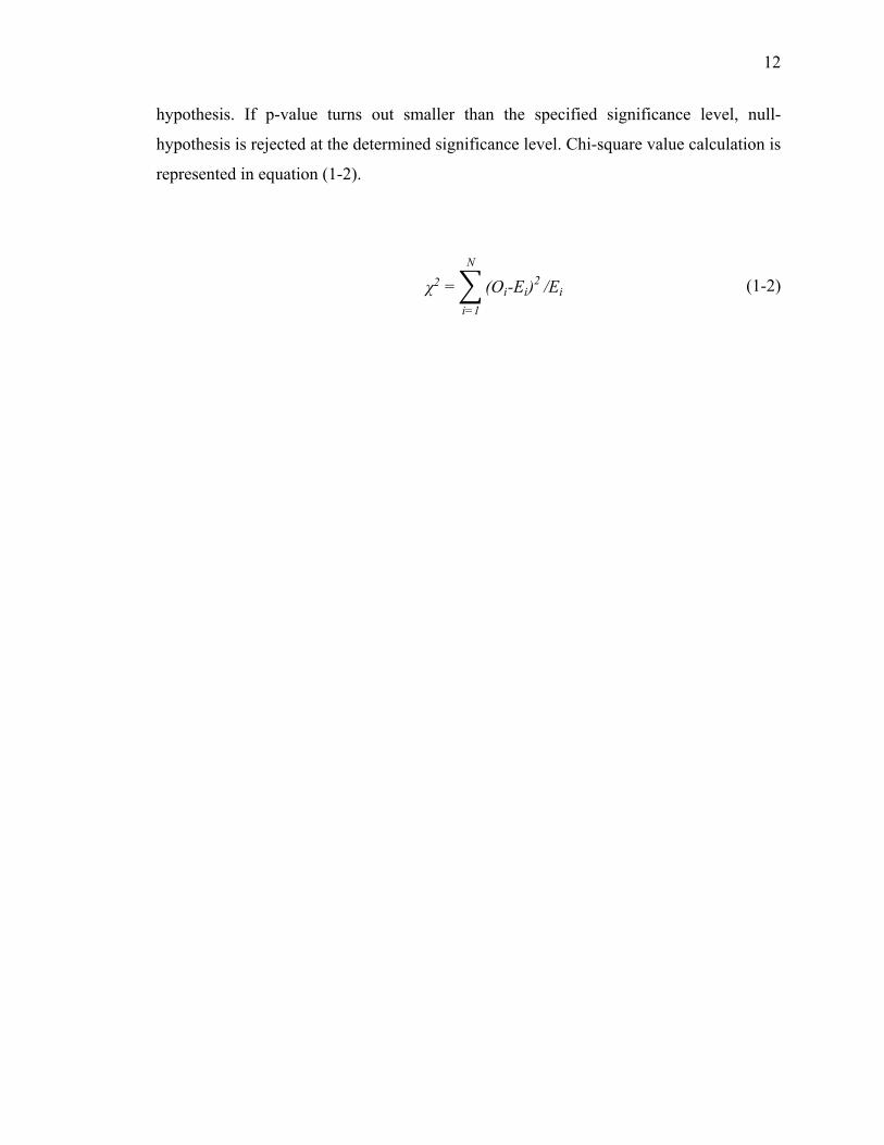
hypothesis. If p-value turns out smaller than the specified significance level, null-
hypothesis is rejected at the determined significance level. Chi-square value calculation is
represented in equation (1-2).
χ2 = (Oi-Ei)2N
i=1
/Ei (1-2)

13
1.3 Treatment Strategies
1.3.1 Pavement Maintenance Terminology
Treatment strategies are commonly categorized in accordance with AASHTO
definitions. The most commonly defined categories include Preventive Maintenance,
Pavement Rehabilitation, and Pavement Reconstruction.
AASHTO states preventive maintenance as “the planned strategy of cost-effective
treatments to an existing roadway system and its appurtenances that preserves the system,
retards future deterioration, and maintains or improves the functional conditions of the
system without increasing structural capacity.” It should be noted that treatments are
categorized as preventive when applied to preserve the pavement. Same action items
applied on a deteriorated pavement are no longer preventive and are categorized as
corrective strategies.
AASHTO Highway Subcommittee on Maintenance also defines Pavement
Rehabilitation as "structural enhancements that extend the service life of an existing
pavement and/or improve its load carrying capacity. Rehabilitation techniques include
restoration treatments and structural overlays”. Finally, Pavement Reconstruction is
outlined as the complete removal and replacement of the existing structure with either
recycled or new materials. Reconstruction is implemented when the pavement fails or
becomes functionally obsolete [17].
The efficiency of these treatment strategies varies significantly within the context of
their application. Mentioned below are the most common influential factors that lead to
choosing one or a group of treatment strategies over another: [12, 16]
• Type and level of distress
• Pavement type and condition
• Load factors including traffic and functional class of the road
• Expected service life of network

14
• Environmental factors such as climate
• Availability of material
• Costs and budget restraints
• Traffic and facility interruption
• Capability of contractors and experience with treatments
• Agency jurisdictions and political issues
Evaluating the success of each treatment strategy is crucial for administration
planning and decision-making. Next section describes the most widely used analysis
methods for evaluating the cost-effectiveness of treatment strategies.
1.3.2 Cost-Effectiveness Analysis And Evaluation
Effectiveness of treatment strategies can be evaluated with various analysis methods.
Significant measures of assessing the effectiveness of treatment strategies that are
accommodated in different analysis methods are financial consequences, maintained
network quality or increased average pavement condition, life extension, and increased
area under performance curve comparing to a base alternative which is classically “do
nothing” [14].
LCCA is best used for evaluating financial consequences of pavement maintenance
strategies over the analysis period, and assessing the competence of each alternative in
terms of Net Present Value or other scales [2]. Hence, the remainder of this chapter aims
to provide a performance-based analysis of consequences of treatment strategies in terms
of cost, remaining service life, and network quality.
1.3.3 Financial Consequences Of Treatment Strategies
Numerous studies have analyzed the impacts of treatment strategies on LCCA
(Zaniewski et al. 2009; Lamptey et al. 2004; Peshkin et al. 2004;)[ 8,6,11]. Other Studies
also show economic value on implementing rehabilitation strategies once or twice prior
to reconstruction [5]. Rajagopal et al. (1990) [7] performed LCCA analysis of three types

15
of treatments applied at different pavement conditions and found that life cycles are
immensely increased when treatments are applied while pavement is experiencing a slow
deterioration rate.
In this study, using LCCA, NPVs of different treatment strategies in cities of
Concord and Norwalk were obtained. Results are then evaluated based on the distinctions
of practices in the two cities. Furthermore, the analysis provides a baseline for evaluating
successful strategies based on NPV values.
Based on Figure 1-6 (a) in analysis of Concord, when NPV is limited to small
values, preventive maintenances provide the highest probability of meeting the budget
criteria. Also, as shown by Figure 1-6 (b) implementing preventive activities yield the
lowest costs during the analysis period, at any given risk. LCCA in concord indicates that
implementing corrective repairs is costly. Corrective repairs do not enhance the structural
capacity. Consequently, while crack seals and thin overlays as preventive strategies
performed at high PCIs are cost-effective, same action items executed as corrective
alternatives at lower PCIs do not eliminate the need of rehabilitation.

16
Figure 1-6. Financial Consequences of Treatment Strategies in Concord
(a) Probability Density Function Of NPV ($$/SY)
(b) Cumulative Probability Of NPV ($$/SY)
0 2 4 6 8 10 12 14 160
0.1
0.2
0.3
0.4
0.5
NPV($$/SY)
Den
sity
Preventive PreventiveP&R P&RP&C&R P & C & R
2 4 6 8 10 12 140
0.1
0.2
0.3
0.4
0.5
0.6
0.7
0.8
0.9
1
NPV($$/SY)
Cum
ulat
ive
prob
abili
ty
Preventive PreventiveP&R P&RP&C&R P & C & R
17
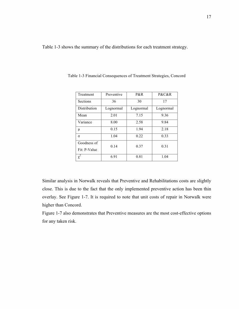
Table 1-3 shows the summary of the distributions for each treatment strategy.
Table 1-3 Financial Consequences of Treatment Strategies, Concord
Treatment Preventive P&R P&C&R
Sections 36 30 17
Distribution Lognormal Lognormal Lognormal
Mean 2.01 7.15 9.36
Variance 8.00 2.58 9.84
µ 0.15 1.94 2.18
σ 1.04 0.22 0.33
Goodness of
Fit: P-Value 0.14 0.37 0.31
χ2 6.91 0.81 1.04
Similar analysis in Norwalk reveals that Preventive and Rehabilitations costs are slightly
close. This is due to the fact that the only implemented preventive action has been thin
overlay. See Figure 1-7. It is required to note that unit costs of repair in Norwalk were
higher than Concord.
Figure 1-7 also demonstrates that Preventive measures are the most cost-effective options
for any taken risk.

18
Figure 1-7 Financial Consequences of Treatment Strategies, Norwalk
(a) Probability Density Function Of NPV ($$/SY)
(b) Cumulative Probability Of NPV ($$/SY
0 5 10 15 20 25 30 35 400
0.02
0.04
0.06
0.08
0.1
0.12
0.14
0.16
NPV($$/SY)
Den
sity
Preventive PreventiveRehabilitation RehabilitationP&R P&RC&R C&R
0 5 10 15 20 25 30 35 400
0.2
0.4
0.6
0.8
1
NPV($$/SY)
Cum
ulat
ive
prob
abilit
y
Preventive PreventiveRehabilitation RehabilitationP&R P&RC&R C&R
19
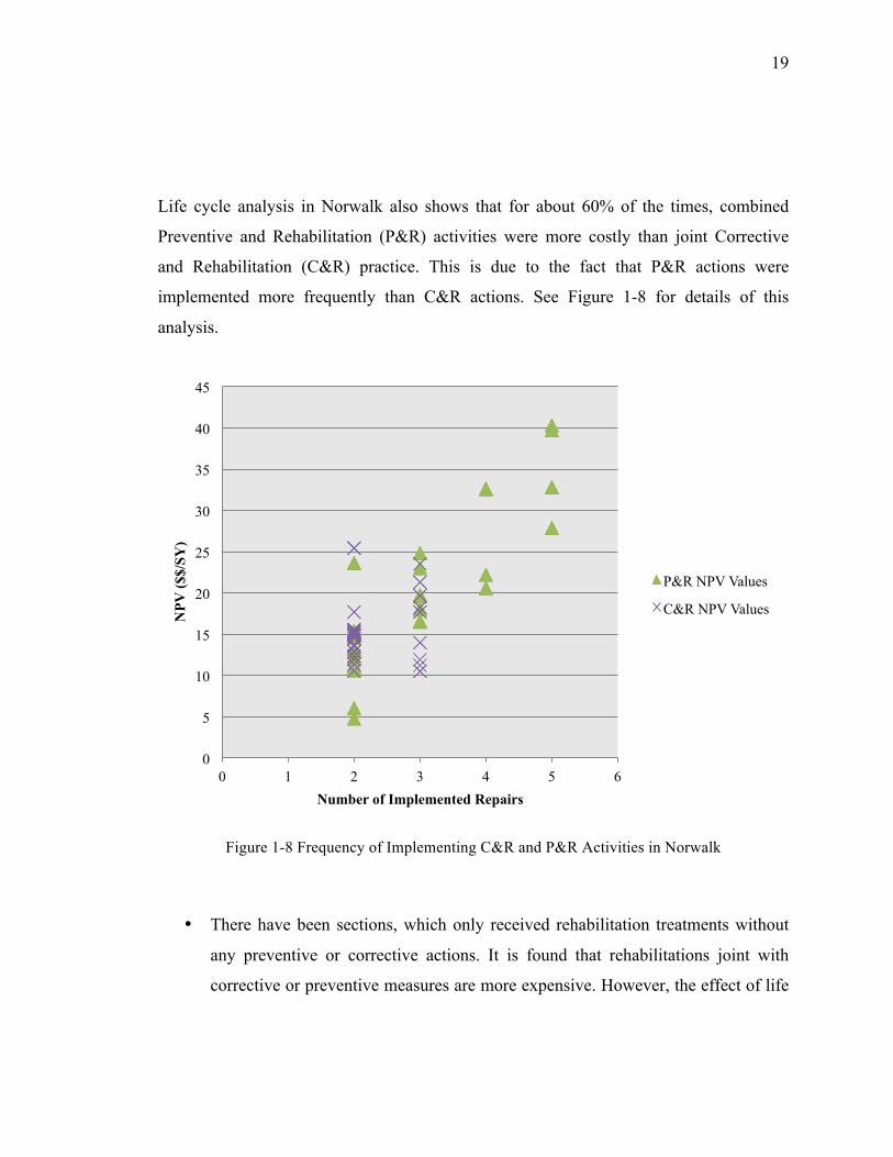
Life cycle analysis in Norwalk also shows that for about 60% of the times, combined
Preventive and Rehabilitation (P&R) activities were more costly than joint Corrective
and Rehabilitation (C&R) practice. This is due to the fact that P&R actions were
implemented more frequently than C&R actions. See Figure 1-8 for details of this
analysis.
Figure 1-8 Frequency of Implementing C&R and P&R Activities in Norwalk
• There have been sections, which only received rehabilitation treatments without
any preventive or corrective actions. It is found that rehabilitations joint with
corrective or preventive measures are more expensive. However, the effect of life
0
5
10
15
20
25
30
35
40
45
0 1 2 3 4 5 6
NPV
($$/
SY)
Number of Implemented Repairs
P&R NPV Values
C&R NPV Values

20
extension will be discussed in next section to evaluate the effectiveness from
other perspectives.
Table 1-4 provides a summary of distribution of treatment strategies costs in Norwalk.
Table 1-4 Financial Consequences of Treatment Strategies, Norwalk
Treatment Preventive P&R C&R Rehabilitation
Sections 29 38 30 32
Distribution Lognormal Lognormal Lognormal Lognormal
Mean 9.57 18.37 15.55 10.16
Variance 16.55 87.87 14.42 10.20
µ 2.18 2.79 2.71 2.27
σ 0.41 0.48 0.24 0.31
Goodness of
Fit: P-Value 0.13 0.62 0.56 0.17
χ2 4.11 0.96 5.86 3.54
Equation ( 1-1 ) can be used for probability density function of Lognormal distribution:
y = f x µ , σ = 1
xσ 2πe-(lnx-µ)2
2σ2 ( 1-1 )
Where,
µ = Log mean
σ = Log standard deviation

21
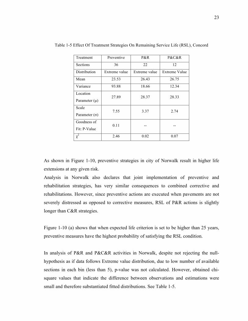
1.3.4 Effect Of Treatment Strategies On Remaining Service Life
Remaining service life is one of the important factors of measuring effectiveness of
treatment strategies. Preventive maintenances applied before drastic distresses, decelerate
the deterioration and extend the serviceability of pavements. However, These
maintenances are non-structural and do not increase the structural integrity of the
pavements. On the other hand, Rehabilitations are applied when pavements are already
distressed. Due to this fact, despite the structural solidification provided by
rehabilitations, deterioration rate will be still ascending. Studies have shown that
preventive maintenances are associated with extending pavement life per unit investment
[14].
As explained earlier in the basis of analysis, remaining service life of sections with
various treatment strategies was calculated comparing to the baseline section that first
reaches its terminal life during analysis period. Results of these analyses in Concord and
Norwalk are subsequently discussed.

22
Figure 1-9 Effect Of Treatment Strategies On Remaining Service Life (RSL), Concord
Figure 1-9 (b) indicates that about 70% of the times combination of rehabilitations with
preventive or corrective actions provides longer remaining service life comparing to
preventive actions in City of Concord. This is due to the fact that rehabilitations are
structural repairs and significantly enhance the remaining service life whereas crack
seals, despite keeping distresses at a low level, do not improve structural capacity.
However, further analysis in city of Norwalk substantiates that preventive actions when
performed as thin-overlay, can be the most effective strategy in extending remaining
service life. Distribution details of Concord analysis are provided in Table 1-5.
(a) Probability Density Function Of RSL (Years)
(b) Cumulative Probability Of RSL (Years)
0 10 20 300
0.02
0.04
0.06
0.08
0.1
0.12
0.14
Remaining Service Life (Years)
Den
sity
Preventive PreventiveP&R P&RP&C&R P&C&R
0 10 20 300
0.2
0.4
0.6
0.8
1
Remaining Service Life (Years)
Cum
ulat
ive
prob
abilit
y
Preventive PreventiveP&R P&RP&C&R P&C&R
23
Table 1-5 Effect Of Treatment Strategies On Remaining Service Life (RSL), Concord
Treatment Preventive P&R P&C&R
Sections 36 22 12
Distribution Extreme value Extreme value Extreme Value
Mean 23.53 26.43 26.75
Variance 93.88 18.66 12.34
Location
Parameter (µ) 27.89 28.37 28.33
Scale
Parameter (σ) 7.55 3.37 2.74
Goodness of
Fit: P-Value 0.11 -- --
χ2 2.46 0.02 0.07
As shown in Figure 1-10, preventive strategies in city of Norwalk result in higher life
extensions at any given risk.
Analysis in Norwalk also declares that joint implementation of preventive and
rehabilitation strategies, has very similar consequences to combined corrective and
rehabilitations. However, since preventive actions are executed when pavements are not
severely distressed as opposed to corrective measures, RSL of P&R actions is slightly
longer than C&R strategies.
Figure 1-10 (a) shows that when expected life criterion is set to be higher than 25 years,
preventive measures have the highest probability of satisfying the RSL condition.
In analysis of P&R and P&C&R activities in Norwalk, despite not rejecting the null-
hypothesis as if data follows Extreme value distribution, due to low number of available
sections in each bin (less than 5), p-value was not calculated. However, obtained chi-
square values that indicate the difference between observations and estimations were
small and therefore substantiated fitted distributions. See Table 1-5.

24
Figure 1-10 Effect Of Treatment Strategies On Remaining Service Life (RSL), Norwalk
(a) Probability Density Function Of RSL (Years)
(b) Cumulative Probability Of RSL (Years)
0 10 20 300
0.02
0.04
0.06
0.08
0.1
0.12
0.14
0.16
Remaining Service Life (Years)
D
ensi
tyPreventive PreventiveRehabilitation RehabilitationP&R P&RC&R C&R
0 10 20 300
0.2
0.4
0.6
0.8
1
Remaining Service Life (Years)
Cum
ulat
ive
prob
abilit
y
Preventive PreventiveP&R P&RC&R C&RRehabilitation Rehabilitation
25
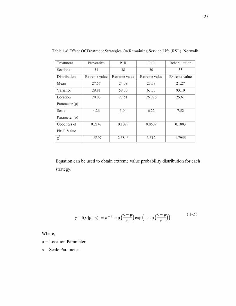
Table 1-6 Effect Of Treatment Strategies On Remaining Service Life (RSL), Norwalk
Treatment Preventive P+R C+R Rehabilitation
Sections 31 38 30 33
Distribution Extreme value Extreme value Extreme value Extreme value
Mean 27.57 24.09 23.38 21.27
Variance 29.81 58.00 63.73 93.10
Location
Parameter (µ)
20.03 27.51 26.976 25.61
Scale
Parameter (σ)
4.26 5.94 6.22 7.52
Goodness of
Fit: P-Value
0.2147 0.1079 0.0609 0.1803
χ2 1.5397 2.5846 3.512 1.7955
Equation can be used to obtain extreme value probability distribution for each
strategy.
y = f x µ , σ = 𝜎! ! expx − µσ
exp −expx − µσ
( 1-2 )
Where,
µ = Location Parameter
σ = Scale Parameter

26
Lastly difference of practice in two cities, leads to the following conclusions:
• Analysis of RSL in two cities shows different effectiveness of treatment
strategies. This is due to the fact that preventive strategies in Norwalk included
only thin-overlay, while Concord has practiced both thin-overlay and crack seal.
• The fact that crack seals are temporarily non-structural treatments substantiates
the difference in effectiveness of preventive strategies. It can be distilled from the
analysis that thin-overlays are more effective than crack seals in terms of life
extension of roads.
1.3.6 Effect Of Treatment Strategies On Network Quality
As mentioned earlier, preventive maintenance is applied when pavements are at incipient
stages of distress. Zaniewski et al. [16] remarks this issue by stating, “Treatments must be
applied in time to preserve the pavement’s structure. Treating distressed pavements is not
preventive maintenance”. These declarations substantiate that preventive maintenances
lead to higher pavement qualities. Whereas allowing pavement condition to reach
rehabilitation thresholds, means pavement experiences lower qualities during its service
life. In addition, studies also show that preventive maintenances yield higher pavement
qualities at lower costs [16].

27
Therefore, this part of analysis is focused on effect of treatment strategies on average
maintained PCI of the network, as well as the worst experienced pavement conditions due
to each strategy.
Average and minimum maintained PCI in Concord are shown in Figure 1-11 and
Figure 1-12 . As expected, preventive strategies provide the highest average PCI at any
given risk. It is notable that in this well-maintained network (in terms of PCI), about 44%
of the network is maintained with preventive strategies. Analysis of the worst network
quality (minimum PCI) is even more sensitive to treatment strategies. Concord analysis
reveals that treatment strategies can change worst PCI values by 25%. In fact, at any
given risk, worst condition of preventive measures is 25% higher than worst condition of
combined preventive, corrective and rehabilitation strategy. Detailed results are further
provided.
Table 1-7 Effect Of Treatment Strategies on Average Network Quality (PCI), Concord
Treatment Preventive P+R PCR
Sections 36 30 17
Distribution Extreme Value Extreme Value Extreme Value
Mean 87.62 86.25 81.94
Variance 16.65 12.896 13.99
Location
Parameter (µ) 89.46 87.86 83.62
Scale
Parameter (σ) 3.18 2.8 2.915
Goodness of
Fit: P-Value 0.5566 0.5578 0.8678
χ2 0.1719 2.0709 0.2836

28
Table 1-8 Effect Of Treatment Strategies on Minimum Network Quality (PCI), Concord
Treatment Preventive P+R PCR
Sections 36 30 17
Distribution Extreme value Extreme value Extreme value
Mean 76.06 68.91 54.10
Variance 70.67 107.95 77.99
Location
Parameter (µ) 79.84 73.59 58.07
Scale
Parameter (σ) 6.55 8.1 6.88
Goodness of
Fit: P-Value 0.4436 0.1263 0.4009
χ2 8.93 2.3371 4.037
Very similar to analysis in Concord, analysis in Norwalk also indicates that preventive
measures provide the highest average and minimum network quality at any given risk.
Furthermore, the analysis indicates that sections treated with preventive and rehabilitation
strategies, experience higher average and minimum PCIs comparing to sections
maintained with combined preventive, corrective and rehabilitation measures. This
substantiates the claim that roads experience lower average and minimum quality over
the analysis period when maintained with corrective strategies.

29
Figure 1-11 Average Network Quality (PCI) Of Treatment Strategies, Concord
(a) Probability Density Function Of PCI
(b) Cumulative Probability Of PCI
0 20 40 60 80 1000
0.02
0.04
0.06
0.08
0.1
0.12
Average Maintained PCI
Den
sity
Preventive PreventiveP&R P&RP&C&R P&C&R
0 20 40 60 80 1000
0.1
0.2
0.3
0.4
0.5
0.6
0.7
0.8
0.9
1
Average Maintained PCI
Cum
ulat
ive
prob
abilit
y
Preventive PreventiveP&R P&RP&C&R P&C&R

30
Figure 1-12 Minimum Network quality (PCI) of treatment strategies, Concord
(a) Probability Density Function Of Minimum PCIs
(b) Cumulative Probability Of Minimum PCIs
0 20 40 60 80 1000
0.01
0.02
0.03
0.04
0.05
0.06
0.07
Minimum Network Quality of Treatment Strategies (PCI)
Den
sity
Preventive PreventiveP&R P&RP&C&R P&C&R
0 20 40 60 80 1000
0.2
0.4
0.6
0.8
1
Minimum Network Quality of Treatment Strategies (PCI)
Cum
ulat
ive
prob
abilit
y
Preventive PreventiveP&R P&RP&C&R P&C&R

31
Figure 1-13 Average Network Quality Of Treatment Strategies (PCI), Norwalk
(a) Probability Density Function Of PCI
(b) Cumulative Probability Of PCI
0 20 40 60 80 1000
0.02
0.04
0.06
0.08
0.1
0.12
0.14
0.16
Average Maintained PCI
Dens
ity
Preventive PreventiveRehabilitation RehabilitationP&R P&RC&R C&R
0 20 40 60 80 1000
0.2
0.4
0.6
0.8
1
Average Maintained PCI
Cum
ulat
ive p
roba
bility
Preventive PreventiveRehabilitation RehabilitationP&R P&RC&R C&R

32
Figure 1-14 Minimum Network quality (PCI) of treatment strategies, Norwalk
(a) Probability Density Function Of Minimum PCIs
(b) Cumulative Probability Of Minimum PCIs
0 20 40 60 80 1000
0.05
0.1
0.15
Minimum Network Quality of Treatment Strategies (PCI)
Den
sity
Preventive PreventiveRehabilitation RehabilitationP&R P&RC&R C&R
0 20 40 60 80 1000
0.2
0.4
0.6
0.8
1
Minimum Network Quality of Treatment Strategies (PCI)
Cum
ulat
ive
prob
abilit
y
Preventive PreventiveRehabilitation RehabilitationP&R P&RC&R C&R

33
Table 1-9 Effect Of Treatment Strategies on Average Network Quality (PCI), Norwalk
Treatment Preventive P+R C+R Rehabilitation
Sections 31 38 30 33
Distribution Extreme Value Extreme Value Extreme Value Extreme Value
Mean 87.46 85.24 75.82 82.64
Variance 12.57 10.51 43.329 22.63
Location
Parameter (µ) 89.05 86.69 78.79 84.78
Scale
Parameter (σ) 2.76 2.53 5.13 3.71
Goodness of
Fit: P-Value 0.8468 0.7728 0.1015 0.3544
χ2 1.3847 1.7981 2.682 3.2522
Table 1-10 Effect Of Treatment Strategies on Minimum Network Quality (PCI), Norwalk
Treatment Preventive P+R C+R Rehabilitation
Sections 31 38 30 33
Distribution Extreme Value Extreme Value Extreme Value Extreme Value
Mean 76.15 70.55 49.96 65.388
Variance 15.93 27.55 332.365 50.835
Location
Parameter (µ) 77.94 72.92 58.166 68.5977
Scale
Parameter (σ) 3.11 4.09 14.216 5.559
Goodness of
Fit: P-Value 0.4217 0.415 0.1827 0.5606
χ2 2.8111 1.7587 1.7757 2.0572

34
1.4 Monitoring Frequency
Monitoring of the network provides invaluable data that if utilized, can
significantly improve performance prediction and PMS decisions. Few studies have
accentuated the importance of a reliable up-to-date database. Smith et al. (2005) [5]
mentions that an improved database is substantial for estimation of rehabilitation
performance. Haider et al. (2011) [3] studied the impact of monitoring frequency on PMS
decisions. The results indicated that when data had a noticeable variability over time (i.e.,
rutting data), monitoring interval had a prominent effect on performance prediction and
consequently influenced PMS decisions.
Finally, monitoring frequency drastically impacts the identification of pre-distress
conditions or existing distresses. These identifications consequently affect the entire PMS
decision-making process in the realms of performance prediction models and priorities in
assigning treatment strategies. Therefore, the remainder of this chapter is focused on
identifying the impact of monitoring frequency on overall life cycle cost, remaining
service life, and network quality.
1.4.1 Cost-Effectiveness Of Monitoring Frequency
Monitoring frequency has complicated implications on cost. On one hand, there
are costs associated with frequent inspection of roads in terms of time and resources. On
the other hand, shorter monitoring intervals provide more reliable assessment of road
conditions, which lead to cost-effective decisions. While only a few studies have focused
on monitoring frequency, Haider et al. (2011) [3] addressed this issue by mentioning the
effect of monitoring frequency on identifying project boundaries, timings, optimum
treatment strategies, and their outcomes on cost-effectiveness.
In this study, after performing LCCA analysis on all arterial sections of the
network, NPV values were categorized based on the inspection frequency of each section.
Distributions of financial consequences of monitoring frequencies in terms of NPV
($$/SY) in Concord in are shown in Figure 1-15. Results of similar analysis in Norwalk
are presented in Figure 1-16.

35
Analysis in Concord Figure 1-15(a) shows that when budget is limited to lower values, 3-
year monitoring frequency has higher probability of meeting the budget criterion as
opposed to 4-year monitoring intervals. Figure 1-15 (b) also indicates that at any given
risk, cost of 3-year monitoring frequency is lower than that of 4-years.
Similar conclusion can be extracted from the analysis in Norwalk based on Figure 1-16.
When budget is limited to smaller values, 3-year, 4-year, and 5-year monitoring intervals
have coordinately higher to lower probabilities of meeting the expenditure limit. Also,
based on Figure 1-16(b), for any acceptable risk, 3-year monitoring frequency results in
lowest and 5-year in highest NPV values. Details of distributions are subsequently
presented.

36
Figure 1-15 Financial Consequences (NPV $$/SY) Of Monitoring Frequency, Concord
(a) Probability Density Function Of NPV ($$/SY)
(b) Cumulative Probability Of NPV ($$/SY)
0 20 40 60 80 1000
0.01
0.02
0.03
0.04
0.05
0.06
Financial Consequences of Monitoring Frequency ($$/SY)
Den
sity
3Yrs 3Yrs4Yrs 4Yrs
0 20 40 60 80 1000
0.2
0.4
0.6
0.8
1
Financial Consequences of Monitoring Frequency ($$/SY)
Cum
ulat
ive
prob
abilit
y
3Yrs 3Yrs4Yrs 4Yrs

37
Table 1-11 Financial Consequences (NPV $$/SY) Of Monitoring Frequency, Concord
Monitoring
Frequency 3Yrs 4Yrs
Sections 62 39
Distribution Lognormal Log-Logistic
Mean 28.68 37.13
Variance 3793.38 inf
Location
Parameter (µ) 2.49 2.93
Scale
Parameter (σ) 1.31 0.5998
Goodness of
Fit: P-Value 0.0694 0.0811
χ2 3.296 3.0419
Table 1-12 Financial Consequences (NPV $$/SY) Of Monitoring Frequency, Norwalk
Monitoring
Frequency 3Yrs 4Yrs 5Yrs
Sections 30 70 39
Distribution Lognormal Lognormal Lognormal
Mean 38.01 42.11 46.49
Variance 1799.64 1353.68 984.33
Location
Parameter (µ) 3.23 3.46 3.65
Scale
Parameter (σ) 0.8994 0.75 0.612
Goodness of
Fit: P-Value 0.6343 0.3 0.0988
χ2 2.5581 3.6638 2.7249

38
Figure 1-16 Financial Consequences (NPV $$/SY) Of Monitoring Frequency, Norwalk
(a) Probability Density Function Of NPV ($$/SY)
(b) Cumulative Probability Of NPV ($$/SY)
0 50 100 150 2000
0.005
0.01
0.015
0.02
0.025
Financial Consequences of Monitoring Frequency ($$/SY)
Den
sity
3Yrs 3Yrs4Yrs 4Yrs5Yrs 5Yrs
0 50 100 150 2000
0.2
0.4
0.6
0.8
1
Financial Consequences of Monitoring Frequency ($$/SY)
Cum
ulat
ive
prob
abilit
y
5Yrs 5Yrs4Yrs 4Yrs3Yrs 3Yrs

39
1.4.2 Effect of Monitoring Frequency on Remaining Service life
As mentioned earlier, monitoring frequency impacts the performance prediction,
distress identification, treatment strategies, PMS decisions, and therefore service life of
the network. Smith et al. [5] in FHWA report of 2005 from Arizona Department of
Transportation recommends biennial analyses for more accurate performance prediction
and estimations of pavement life.
In this sub-chapter of life cycle analysis, remaining service life comparing to the
base road segment that reaches its terminal life was calculated, and categorized for each
monitoring frequency to obtain probability distributions.
Consequences of monitoring frequencies on Remaining Service Life (RSL) in cities of
Concord and Norwalk are accordingly presented in Figure 1-17and Figure 1-18.
In analysis of Concord network, Figure 1-17 indicates that for any given risk, 3-
year monitoring interval provides higher RSL comparing to 4-year inspections.
Similar analysis in Norwalk’s network indicates that while 3-year and 4-year
monitoring frequencies are close in results, yet at any given risk, 3-year inspection
frequency results in the highest and 5-year frequency in lowest values of remaining
service life.
It is required to note that due to lack of data points in Concord for 4-year
monitoring interval, p-value could not be calculated for RSL. However, since the null-
hypothesis was not rejected and the calculated chi-square value was 7.5%, extreme value
distribution was considered appropriate for this category of data.

40
Figure 1-17 Remaining Service Life (RSL) Of Monitoring Frequencies, Concord
(a) Probability Density Function Of RSL (Years)
(b) Cumulative Probability Of RSL (Years)
0 5 10 15 20 25 30 35 40 450
0.01
0.02
0.03
0.04
0.05
0.06
Remaining Service Life (RSL), Years
Den
sity
3Yrs 3Yrs4Yrs 4Yrs
0 5 10 15 20 25 30 35 40 450
0.2
0.4
0.6
0.8
1
Remaining Service Life (RSL), Years
Cum
ulat
ive
prob
abilit
y
3Yrs 3Yrs4Yrs 4Yrs

41
Table 1-13 Remaining Service Life (RSL) Of Monitoring Frequencies, Concord
Monitoring
Frequency 3Yrs 4Yrs
Sections 47 21
Distribution Extreme Value Extreme Value
Mean 19.90 10.13
Variance 140.00 313.503
Location
Parameter (µ) 25.22 18.10
Scale
Parameter (σ) 9.225 13.805
Goodness of
Fit: P-Value 0.0824 --
χ2 3.0161 0.0751
Table 1-14 Remaining Service Life (RSL) Of Monitoring Frequencies, Norwalk
Monitoring
Frequency 3Yrs 4Yrs 5Yrs
Sections 31 70 40
Distribution Extreme
value
Extreme
value
Extreme
Value
Mean 24.99 24.42 22.46
Variance 50.43 47.66 83.79
Location
Parameter (µ) 28.1865 27.53 26.5771
Scale
Parameter (σ) 5.537 5.38 7.1369
Goodness of
Fit: P-Value 0.1908 0.266 0.1482
χ2 1.7113 3.9581 2.0902

42
Figure 1-18 Remaining Service Life (RSL) Of Monitoring Frequencies, Norwalk
(a) Probability Density Function Of RSL (Years)
(b) Cumulative Probability Of RSL (Years)
0 5 10 15 20 25 30 35 40 450
0.02
0.04
0.06
0.08
Remaining Service Life (RSL), Years
D
ensi
ty3Yrs 3Yrs4Yrs 4Yrs5Yrs 5Yrs
0 5 10 15 20 25 30 35 40 450
0.2
0.4
0.6
0.8
1
Remaining Service Life (RSL), Years
Cum
ulat
ive
prob
abilit
y
3Yrs 3Yrs4Yrs 4Yrs5Yrs 5Yrs

43
1.4.3 Effect of Monitoring Frequency on Network Quality
Monitoring frequency can affect network quality on different levels of PMS.
These aspects include identification of distresses, planning for appropriate maintenance
strategies, and implementation of planned treatments. Each of these phases directly
impacts the network quality.
Studies have shown that when inspections are performed more frequently, higher
rates of distress growth is captured [3]. McGhee et al. [18] emphasizes the necessity of
monitoring distress quantities on a year-to-year basis. Furthermore, pavement segments
that require repairs have lower chances of being captured when monitoring intervals are
longer. The other shortcoming of less frequent monitoring is that when section is
recognized for treatment, the distress might already be severe. Therefore, the repair
would be more costly, the remaining service life would be shorter, and the road section
experiences poorer qualities before being repaired.
This part of the analysis is focused on consequences of monitoring intervals on average
and minimum experienced PCI of Concord and Norwalk Network.
As shown by Figure 1-19, 3-year and 4-year monitoring intervals have close
consequences in terms of average maintained condition. Yet, it is still evident that for any
taken risk, average PCI of 3-year monitoring intervals are slightly higher than 4-year
frequency.
However, analysis of minimum PCI in Concord, as presented in Figure 1-20 ,
indicates that about 70% of the times, 3-year monitoring frequency has higher
probabilities of satisfiying the minimum PCI criterion comparing to 4-year inspection
frequency.
Similar analysis in Norwalk indicates that average maintained PCI of monitoring
frequencies are slightly close while longer frequencies have lower average PCIs at any
given risk. See Figure 1-21.
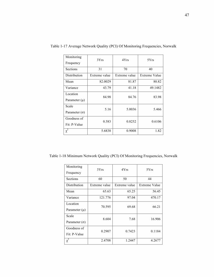
Further analysis of minimum PCI in Norwalk in Figure 1-22 indicates more
significant impact of monitoring frequency. 80% of the times, 5-year monitoring
frequency results in 20% lower PCI values. Details of the distributions are accordingly
provided in Table 1-15 to Table 1-18.

44
Figure 1-19 Average Network Quality (PCI) Of Monitoring Frequencies, Concord
(a) Probability Density Function Of PCI
(b) Cumulative Probability Of PCI
0 20 40 60 80 1000
0.02
0.04
0.06
0.08
0.1
Network Quality of Monitoring Frequencies (PCI)
Den
sity
3Yrs 3Yrs4Yrs 4Yrs
0 20 40 60 80 1000
0.2
0.4
0.6
0.8
1
Network Quality of Monitoring Frequencies (PCI)
Cum
ulat
ive
prob
abilit
y
3Yrs 3Yrs4Yrs 4Yrs

45
Figure 1-20 Minimum Network Quality (PCI) Of Monitoring Frequencies, Concord
(a) Probability Density Function Of Minimum PCIs
(b) Cumulative Probability Of Minimum PCIs
0 20 40 60 80 1000
0.005
0.01
0.015
0.02
0.025
0.03
0.035
Minimum Network Quality of Monitoring Frequencies (PCI)
Den
sity
3Yrs 3Yrs4Yrs 4Yrs
0 20 40 60 80 1000
0.2
0.4
0.6
0.8
1
Minimum Network Quality of Monitoring Frequencies (PCI)
Cum
ulat
ive
prob
abilit
y
3Yrs 3Yrs4Yrs 4Yrs

46
Table 1-15 Average Network Quality (PCI) Of Monitoring Frequencies, Concord
Monitoring
Frequency 3Yrs 4Yrs
Sections 78 21
Distribution Extreme value Extreme value
Mean 85.83 85.38
Variance 20.30 25.08
Location
Parameter (µ) 87.86 87.63
Scale
Parameter (σ) 3.51 3.9
Goodness of
Fit: P-Value 0.8959 0.8692
χ2 1.09 1.2539
Table 1-16 Minimum Network Quality (PCI) Of Monitoring Frequencies, Concord
Monitoring
Frequency 3Yrs 4Yrs
Sections 78 21
Distribution Extreme value Lognormal
Mean 66.47 68.78
Variance 179.89 414.00
Location
Parameter (µ) 72.51 4.19
Scale
Parameter (σ) 10.46 0.29
Goodness of
Fit: P-Value 0.5991 0.1843
χ2 1.8732 1.7627
47
Table 1-17 Average Network Quality (PCI) Of Monitoring Frequencies, Norwalk
Monitoring
Frequency 3Yrs 4Yrs 5Yrs
Sections 31 70 40
Distribution Extreme value Extreme value Extreme Value
Mean 82.0029 81.87 80.82
Variance 43.79 41.18 49.1482
Location
Parameter (µ) 84.98 84.76 83.98
Scale
Parameter (σ) 5.16 5.0036 5.466
Goodness of
Fit: P-Value 0.583 0.8252 0.6106
χ2 5.6838 0.9008 1.82
Table 1-18 Minimum Network Quality (PCI) Of Monitoring Frequencies, Norwalk
Monitoring
Frequency 3Yrs 4Yrs 5Yrs
Sections 60 50 44
Distribution Extreme value Extreme value Extreme Value
Mean 65.63 65.25 56.45
Variance 121.776 97.04 470.17
Location
Parameter (µ) 70.595 69.68 66.21
Scale
Parameter (σ) 8.604 7.68 16.906
Goodness of
Fit: P-Value 0.2907 0.7423 0.1184
χ2 2.4708 1.2447 4.2677

48
Figure 1-21 Average Network Quality (PCI) Of Monitoring Frequencies, Norwalk
(a) Probability Density Function Of PCI
(b) Cumulative Probability Of PCI
0 20 40 60 80 1000
0.01
0.02
0.03
0.04
0.05
0.06
0.07
0.08
Network Quality of Monitoring Frequencies (PCI)
Den
sity
3Yrs 3Yrs4Yrs 4Yrs5Yrs 5Yrs
0 20 40 60 80 1000
0.2
0.4
0.6
0.8
1
Network Quality of Monitoring Frequencies (PCI)
Cum
ulat
ive
prob
abilit
y
3Yrs 3Yrs4Yrs 4Yrs5Yrs 5Yrs

49
Figure 1-22 Minimum Network Quality (PCI) Of Monitoring Frequencies, Norwalk
(a) Probability Density Function Of Minimum PCIs
(b) Cumulative Probability Of Minimum PCIs
0 20 40 60 80 1000
0.01
0.02
0.03
0.04
0.05
Minimum Network Quality of Monitoring Frequencies (PCI)
Den
sity
3Yrs 3Yrs4Yrs 4Yrs5Yrs 5Yrs
0 20 40 60 80 1000
0.2
0.4
0.6
0.8
1
Minimum Network Quality of Monitoring Frequencies (PCI)
Cum
ulat
ive
prob
abilit
y
3Yrs 3Yrs4Yrs 4Yrs5Yrs 5Yrs

50
1.4.4 Application of Risk-based approach in management decisions
To demonstrate the application of risk-based analyses previously discussed, this sub-
chapter provides a few examples of pavement management system targets and suggested
solutions. Considering the network of Concord, three various scenarios are presented:
Target 1:
ü Road Condition ≥70
ü Cost ≤ 8($$/SY)
ü Risk ≤ 20%
Figure 1-23 PMS Solution Case-1
RSL
17-32
Years
Treatment
Preventive
RSL Cost PCI
11-30
Years
3-37
($$/SY)
58-78 Monitoring Freq.
3 Years
Suggestions
Outcomes (20% Risk)

51
As illustrated in Figure 1-23 appropriate treatment strategies and required
monitoring frequencies are proposed based on network management goals. Preventive
strategy is recognized as the treatment option, which satisfies all the required criteria.
Consequently, this maintenance option along with other limits set, results in 17 to 32
years of service life. On the other hand, 3-year monitoring frequency sets some limits on
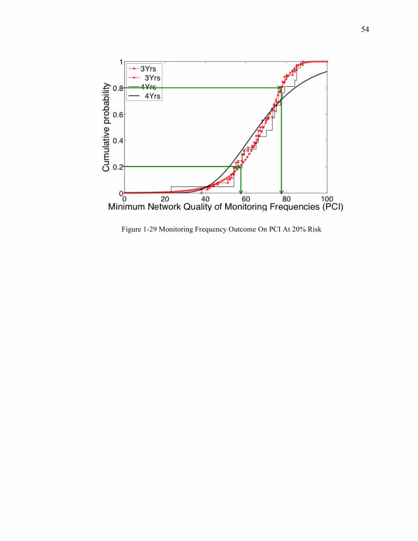
targets. For the assigned 20% acceptable risk, cost and PCI requirements may not be met.
According to Figure 1-23 cost and PCI can vary such that they may or may not satisfy the
limits. Detailed steps for suggestions of Case-1 are further illustrated in Figure 1-24 to
Figure 1-29.
Figure 1-24 Treatment Suggestion To Meet Budget Limit At 20% Risk

52
Figure 1-25 Treatment Suggestion To Meet PCI Limit At 20% Risk
Figure 1-26 Outcome Of Treatment Suggestion On RSL At 20% Risk

53
Figure 1-27 Monitoring Frequency Outcome On RSL At 20% Risk
Figure 1-28 Monitoring Frequency Outcome On Cost At 20% Risk
54
Figure 1-29 Monitoring Frequency Outcome On PCI At 20% Risk

55
Figure 1-30 PMS Solution Case-2
Target 2:
ü Road Condition ≥ 75
ü Cost ≤ 8 ($$/SY)
ü RSL ≥ 30 Years
ü Target 2
Suggestion Outcomes
Monitoring
Frequency
Cost
Risk
PCI
Risk
RSL
Risk
3 Years 60% 75% 85%
4 Years 78% 70% 90%
ü Target 2
Suggestion Outcomes
Treatment Cost
Risk
PCI
Risk
RSL
Risk
Preventive 5% 35% 75%
P&R 20% 75% 90%
P&C&R 65% 100% 95%

56
Figure 1-30 demonstrates a different perspective where goals are set based on condition,
cost, and service life. In this case, various treatment strategies and monitoring frequencies
can be implemented with different risk factors. Also, risk factor for each criterion is
different as presented in outcomes. Decision makers can then decide based on the level of
risk acceptance.
Figure 1-31 PMS Solution Case-3
Target 3:
ü Road Condition ≥ 75
ü Risk ≤ 30%
ü RSL ≥ 20 Years
ü Target 3
Suggestion Outcomes
Monitoring
Frequency
Expected
Cost
PCI
Risk
RSL
Risk
3 Years 5-22
($$/SY)
70% 40%
ü Target 3
Suggestion Outcomes
Treatment Expected Cost
Preventive 0.75-2($$/SY)

57
Last case (Figure 1-31 ) illustrates a situation where cost will be determined based on
accepted risk, road quality, and service life. Preventive maintenance was able to satisfy
the PMS limits with the suggested cost. 3-year monitoring frequency on the other hand,
satisfies PCI and RSL limits at higher risks than initial target. However, possible cost
range of 3-year monitoring frequency is proposed based on the initial 30% risk.

58
1.5 Chapter Summary And Conclusions
This chapter was determined to suggest risk-informed management solutions by
reflecting the tradeoffs between cost and service quality. Probabilistic data-driven LCCA
was leveraged to provide outcomes of various treatment strategies and pavement
monitoring frequency alternatives in terms of cost, remaining service life, and network
quality. The major contributions and findings of this study are summarized bellow:
§ When NPV is limited to small values, preventive maintenances provide the
highest probability of meeting the budget criteria.
§ Implementing preventive activities yield the lowest costs during the analysis
period, at any given risk.
§ Executing corrective repairs is costly. Corrective repairs do not enhance the
structural capacity. Consequently, while crack seals and thin overlays as
preventive strategies performed at high PCIs are cost-effective, same action items
executed as corrective alternatives at lower PCIs do not eliminate the need of
rehabilitation.
§ Rehabilitations are structural repairs and significantly enhance the remaining
service life. Whereas crack seals, despite keeping distresses at a low level, do not
improve structural capacity and therefore service life. However, further analysis
in city of Norwalk substantiates that preventive actions when performed as thin
overlay, can be the most effective strategy in extending remaining service life.

59
Briefly, difference of practice in two cities, leads to the following conclusions in terms of
RSL:
Ø Analysis of RSL in two cities shows different effectiveness of treatment
strategies. This is due to the fact that preventive strategies in Norwalk
included only thin-overlay, while Concord has practiced both thin-overlay and
crack seal.
Ø The fact that crack seals are temporarily non-structural treatments
substantiates the reason for difference in effectiveness of preventive strategies.
It can be distilled from the analysis that thin-overlays are more effective than
crack seals in terms of life extension of roads.
§ Preventive strategies provide the highest average PCI at any given risk.
§ Analysis of the worst network quality (minimum PCI) is more sensitive to
treatment strategies and monitoring frequencies comparing to average PCI.
§ Concord analysis reveals that treatment strategies can change worst PCI values by
25%. In fact, at any given risk, worst condition of preventive measures is 25%
higher than worst condition of combined preventive, corrective and rehabilitation
strategies.
§ When budget is limited, 3-year monitoring frequency has higher probability of
meeting the budget criterion as opposed to 4-year monitoring intervals.
§ 3-year, 4-year, and 5-year monitoring intervals have coordinately higher to lower
probabilities of meeting the expenditure limit.

60
§ For any given risk, 3-year monitoring interval provides higher RSL comparing to
4-year and 5-year inspections.
§ Longer monitoring frequencies have lower average PCIs at any given risk.
§ In 80% of the conditions, 5-year monitoring frequency results in 20% lower
minimum PCI values.
Lastly, to pinpoint the tradeoffs between costs and service quality, benefit to cost
indicators are obtained from mean-value of provided distributions. These indicators are
scaled ratios between average PCI and cost, minimum PCI and cost, and RSL and cost.
Table 1-19 Benefit To Cost Ratios Of Treatment Strategies
Concord Norwalk
Treatment Preventive P+R PCR Preventive Rehabilitation P+R C+R
RSL/Cost 1 0.32 0.24 1 0.73 0.46 0.52
Avg
PCI/Cost 1 0.28 0.20 1 0.89 0.51 0.53
Min
PCI/Cost 1 0.25 0.15 1 0.81 0.48 0.40

61
Table 1-20 Benefit To Cost Ratios Of Monitoring Frequencies
Concord Norwalk
Monitoring
Frequency 3Yrs 4Yrs 3Yrs 4Yrs 5Yrs
RSL/Cost 1 0.39 1 0.88 0.73
Avg
PCI/Cost 1 0.77 1 0.90 0.81
Min
PCI/Cost 1 0.80 1 0.90 0.70
Figure 1-32 Benefit To Cost Ratios Of Treatment Strategies (Table 1-19 )
0 0.1 0.2 0.3 0.4 0.5 0.6 0.7 0.8 0.9
1
Prev
entiv
e
P+R
PCR
Prev
entiv
e
Reh
abili
tatio
n
P+R
C+R
Concord Norwalk
RSL/Cost
Avg PCI/Cost
Min PCI/Cost

62
Figure 1-33 Benefit To Cost Ratios Of Monitoring Frequencies (Table 1-20 )
0 0.1 0.2 0.3 0.4 0.5 0.6 0.7 0.8 0.9
1
3Yrs 4Yrs 3Yrs 4Yrs 5Yrs
Concord Norwalk
RSL/Cost
Avg PCI/Cost
Min PCI/Cost

63
2 PERFORMANCE BASED CONDITION PREDICTION
Effective execution of PMS planning and project prioritization, in addition to
comprehensive up-to-date data and associated risks, drastically depends on the accuracy
of future deterioration prediction.
Prediction of pavement deterioration influences many PMS components such as
determining the rehabilitation time, corresponding treatment alternatives for future years
and selecting the most effective maintenance and rehabilitation (M&R) alternatives [20].
Condition of pavements during and at the end of investment time span significantly
affects budget allocation and prioritization decisions. Therefore, a precise deterioration
model is vital to the success of such immense investment plans.
Lastly, a solid deterioration model will not only helps road controlling authorities in
cost-effective scheduling of maintenance activities and budget allocations, but it can also
be employed for the design of pavement structures. Consequently, these models can be
utilized for evaluation of different design, maintenance, and rehabilitation strategies
based on geographical regions, estimated volumes of traffic and other factors [21].
There are numerous factors that affect the accuracy of deterioration models. Many
efforts have been taken to consider the most influential parameters and provide precise
performance models. In this chapter, first, an overview of influential parameters and
widely used models are presented. Despite all the success, there are still some factors
such as extreme weather events that are overlooked in deterioration models. Therefore,
this chapter aims to provide one of the most cutting edge and inclusive performance
based models for condition prediction.

64
2.1 General Influencing Parameters On Pavement Performance
Interactions between climate, vehicles and the road result in deformation and
deterioration of pavements. Prediction of this behavior is complicated. While
deterioration models for rigid pavements have had a decent performance, because of the
high viscoelastic characteristic of the asphalt, current deterioration models for flexible
pavements have had limited success so far.
Pavement infrastructure deterioration is caused by aggregated impact of traffic
loads, environmental conditions, and other contributors. The behavior of pavement under
these factors depends on the characteristics of its structure (materials and thickness of
each pavement layer), the quality of its construction, and the subgrade (bearing capacity
and presence of water) [22]. Each factor causes certain distresses on the pavement.
Understanding factors that lead to deterioration of roads help infrastructure managers to
refine their construction and maintenance specifications.
Load: Cracking and rutting caused by pavement bending under traffic loads are two of
the most prominent forms of distresses. Tire pressure produced by vehicles in the radius
of loaded area induces tensile stress on the pavement, lateral shear in the surface and
vertical stress at the subgrade, which gradually deteriorate the pavement [23].
Material Properties: Severity of distresses and the pace of their formation are heavily
influenced by material properties of the pavement. Strength and bearing capacity,
gradation, modules of elasticity and resilience of the materials used in construction
determine pavements endurance under load and climate fluctuations [24].
Construction Quality: Freitas et al. [25] shows that construction quality influences the
two significant factors in initiation of top-down cracking: voids and aggregate gradations
caused. Construction quality also determines the initial pavement condition, which has an
impact on the pace that pavement failures occur.
Environmental Conditions: Climate oscillations, precipitation and freeze/thaw cycles
are the primary causes of some dominant distresses such as longitudinal and transversal
cracks [26].

65
• Temperature: Temperature fluctuations are followed by tensile and compressive
stress in pavement, which initiates thermal cracking. Smith et al [27] shows a
correlation between pavement deterioration and temperature where surge in
temperature facilitates rutting and cracking in the pavement.
• Precipitation: Studies on pavement performance evaluations show that other than
formation of longitudinal and alligator cracks, roughness of the road also worsens
with a boost in precipitation.
• Freeze/thaw cycles: In cold regions, water penetrated into the pavement layers
freezes in the winter. Thaw of these ice particles during spring causes deformation
in pavement layers and triggers fatigue cracking [28].
The effects of traffic loads and environmental factors on pavement condition prediction
have been widely studied [28, 29, 30, 31]. Majority of prediction models, regardless of
the applied approach for prediction, have considered to some extent similar factors.
2.2 Condition Prediction/Deterioration Modeling Of Pavements
Depending on how aging of the pavement is simulated, road deterioration models can be
categorized into three main classes of Empirical, Probabilistic, and Mechanistic-
Empirical. Following section explains the basis of these models, their drawbacks and
finally, the proposed methodology.
• Empirical prediction models are typically simple performance models that are
obtained from fitting curves to historic performance data. The Highway
development and Management Tool (HDM-4) is an example of these models that
is widely used for condition prediction and strategic planning of pavements at

66
project and network level [44]. The proposed roughness deterioration model by
HDM-4 is developed based on structural damage to the pavement and change in
roughness due to cracking, rutting, potholing, and environment. This model
requires extensive information on the road network to perform well. Additionally,
it needs to be calibrated for different regions.
• Probabilistic models are typically based on the Markov chain process and work
with transition probability matrices to account for the probability of pavement
condition transitioning from one state to another. MicroPAVER is one of the
widely used tools, which applies this model [45]. While this model is able to
overcome the stochastic characteristics of influential factors on deterioration,
there are some limitations. Establishment of these probability matrices can be
costly and time-consuming as historic data or opinions of expert engineers are
required. Furthermore, applicability of the transition matrix is limited to only
several widely spaced categories typically classified by traffic volume, pavement
structure and climate regions [43]. In addition, time independent stochastic
process of Markov chains, implies that rate of deterioration does not depend on
time [46]. However, many studies have demonstrated that deterioration
accelerates as age of the pavement grows [47].
• Mechanistic-empirical models are based on constitutive laws between mechanical
characteristics of pavements and external factors. In these models, mechanical
characteristics of pavements such as stress-strain relationships are associated with
external elements like traffic loads. Eventually, future pavement condition is
projected using statistical models. National Cooperative Highway Research
Program (NCHRP) has included this type of performance prediction model in the
2002 mechanistic-empirical design guidelines [48].
While these studies have modeled natural deterioration with some level of success, most
have neglected the aggravating effect of extreme weather events.
67
Aftermaths of events such as hurricane Sandy in New York and New Jersey and
hurricane Katrina in New Orleans [49] emphasize the importance of considering extreme
weather events in performance prediction of pavements. Moreover, a study after the
2006/2007 Denver, Colorado snowstorms indicated 16% decline in road conditions [50].
Poor pavement conditions are caused by shear failure, weakening of the subgrade,
cracking, and worsening the severity of existing cracks as a result of extreme weather
events.
Fundamentally, severe floods increase the subgrade’s moisture content and
drastically damage the surface layer. Snowstorms also increase pavement roughness by
inducing thermal cracks and causing uneven frost heaves. In addition, heavy loads of
snow, which sometimes remains on pavements for months, and heavy loads applied by
snow removal vehicles further damage the pavements [51,52].
In this study, efforts have been taken to quantify the effects of extreme weather
events on performance of flexible pavements. Next sections are structured based on data
collection, quantification of extreme events, and development of a regression-based
model for performance prediction in extreme conditions.
2.3 Data & Methodology
In order to conduct a data driven approach for development of a performance
prediction model, pavement condition and extreme weather events data had to be
collected.
Performance data were obtained from the Long Term Pavement Performance (LTPP)
database [53], which contains pavement performance data of over 2,400 pavement
sections throughout the United States and Canada. In addition to performance, traffic and
climatic data were gathered from 8 states of New York, Louisiana, Oregon, Colorado,
New Jersey, Illinois, Ohio, and Florida for an analysis period of 18 years (1996 to 2013).
These states were selected since they encompass the most inclusive datasets and were
specifically affected by significant extreme weather events.

68
Discussions here are focused on using the IRI as the performance measurement of
pavement sections. Typically obtained from longitudinal road profiles, ASTM defines
IRI as “a quantitative estimate of a pavement property defined as roughness using
longitudinal profile measures.”[56] IRI is widely used for evaluating and managing
highways since the early 1980s.
Extreme weather events data were obtained from the National Oceanic and
Atmospheric Administration (NOAA) database [54]. In order to quantify the magnitude
of floods and snowstorms, duration and the reported depth of snow and flooded water
were acquired.
One challenge was to match the LTPP sections corresponding to the county-based
extreme weather events data obtained from NOAA. To make the datasets of two different
references consistent, pavement sections and climate regions were categorized based on
their counties.
In addition, some sections in the LTPP database had insufficient data for two of
the parameters used in the proposed model: Structural Number and Equivalent Single
Axle Load (ESAL). Missing structural numbers were estimated based on the pavement
type, information of layers thicknesses, subgrade moduli, and available structural number
of the adjacent sections with similar characteristics recorded in the LTPP database.
Absent ESAL values were estimated based on traffic counts, number of lanes, and
vehicle axle loads [55].
Performance surveys and models provide natural deterioration information in
annual format. On the other hand, events taking place in zones prone to extreme climate
conditions have a high frequency of occurrence and an instantaneous nature. Therefore,
to effectively capture the effect of events occurring between surveys, a monthly accurate
analysis was required. For that purpose, annual climate and traffic reports of LTPP were
converted into monthly format data.
Lastly, a natural deterioration model was required to capture and quantify the
effect of extreme events. At many cases, multiple extreme events occurred between two
measurements of IRIs. Based on the reports of depth, duration, and property damage, less

69
significant events were filtered out and data points with only one major extreme event
between surveyed IRIs were attained. Data collection procedure is illustrated in Figure
2-1.
Figure 2-1 Data Collection Procedure
Pavement sections collected
from LTPP for 8 states LTPP
collected sections
with flexible
pavements Monthly format
performance,
climate, and traffic
data Events
located on sections collected
from NOAA
Sections with
extreme events
between IRI
surveys
Sections with only
1 significant
event between
IRI surveys
70
Proposed model consists of two parts: A natural deterioration model, and a deterioration
model due to extreme weather events. The first part has been adopted and the latter has
been developed based on the collected data described earlier.
2.3.1 Natural Deterioration Model
To choose an appropriate natural deterioration model based on the availability of
data, some of the widely used models were studied. In a study conducted by Jackson et
al. [28], multivariate regression analysis was implemented on LTPP data test sections
classified as SPS-1, SPS-8, GPS-1, GPS-2, and GPS-6 to propose flexible pavement
performance models. Effects of environmental factors such as freeze cycles and deep
frost penetration, on pavement performance have been considered in this study. A
deterioration model predicting roughness of flexible pavements was proposed as the
following:
Ln ∆IRI+1 =Age(4.5FI+1.78CI+1.09FTC+2.4PRECIP+5.39Log ESAL
SN) (2-1)
Where:
∆IRI : Change in International Roughness Index
Age : Pavement Age
FI : Freezing Index (Degree-days when air temperatures are below and above zero
degrees Celsius)
CI : Cooling Index (Temperature relation to the relative humidity and discomfort)
FTC : Freeze-thaw Cycles

71
PRECIP : Precipitation
ESAL : Equivalent Single Axle Load (Conversion of traffic into single axle load)
SN : Structural Number
This model has leveraged the comprehensive LTPP performance data and predicted the
accumulation of roughness with time with a root mean square error (RSME) of 0.17.
Therefore, this model was chosen as the basic approach for quantifying the effect of
extreme events.
2.3.2 Quantification Of Impact Factor
As mentioned earlier, performance data from LTPP and extreme weather events
data from NOAA are not necessarily synchronized. Quantifying the impact of extreme
weather events needs prediction of performance data to the month the event has occurred.
Natural deterioration model proposed by Jackson et al [28], presented in equation (2-1)
was used to carry this prediction.
Consequently, IRI recorded before an extreme weather event was forward-
projected to the time of the event by natural deterioration model. Then, the IRI value
recorded after the event was backward-projected to the time of the event. Difference
between the forward-projected and the backward-projected IRI values is the additional
deterioration caused by the extreme event occurred in between. The explained
methodology is illustrated in Figure 2-2.

72
Figure 2-3 shows the analysis implemented on a section in Colorado from 1996 to
2013. Points marked with upside triangles represent surveyed IRI values recorded in
LTPP database. Natural deterioration, which is backward and forward projected between
measured IRIs at the time of extreme weather event occurrence, is presented with the
blue-filled prediction line.
Also, measurements of IRIs are connected to each other with the dash line to
illustrate the difference between predicted and surveyed IRI values.
June 2011 (Month 187) is an example of extreme event occurrence as reported with 1 (ft)
of flooding in 1 hour; the predicted IRI value for that month is 1.213 (m/km) while the
actual measurement in less than 2 months later indicates an IRI value of 1.46 (m/km).
Figure 2-2 Quantifying The Impact Of Extreme Events

73
Difference between be the measured and predicted values indicates the impact of the
flood in this specific case. On another note, maintenance actions can also be observed in
this plot. Month 125 is an example of maintenance action where the predicted IRI value
is 1.33 (m/km) and the survey indicates decrease in IRI.
2.3.3 Deterioration In Extreme Conditions
Applying the described methodology, 75 data points were quantified which were
impacted by only one flood or snowstorm in the 1996 to 2013 period. Depth and duration
of the extreme events were chosen as indicators of events’ magnitudes. After observing
the high correlation of traffic (ESAL) and pavement roughness (IRI) with the quantified
impact values, these factors were also considered as possible predictors. Deciding what
algorithm to use depends heavily on the application and what is expected from the fusion
system. Pattern recognition, artificial intelligence and regression are some common
Figure 2-3 Impact Of Extreme Events And Maintenance Actions On Measured And Predicted IRI
Values

74
fusion techniques. Here, an algorithm that is adept at variable selection is required as one
might conclude that not all of these parameters are necessary to predict IRI scores.
Consequently, the high correlation between the predictors and the deterioration rates led
to employing a statistical regression model. Another reason for considering regression is
the limited number of data points, as regression could deal better with them than machine
learning techniques such as Neural Networks [58].
Regression is a statistical tool for exploring relationships between variables that
are related in a nondeterministic manner. Proposed model in this study is Stepwise
Regression. Stepwise regression enters and removes variables one at a time to see
whether it improves the model. Usually, this takes the form of a sequence of F-tests, but
other techniques such as t-tests, adjusted R-square, Bayesian information criterion, or
false discovery rate are also possible [59]. Finally, obtained correlations are presented in
Table 2-1.
Table 2-1 Correlation Of Predictors With Percentage Increase In IRI Due To The Extreme Event
Predictor Correlation with %ΔIRI for Snow Storms Correlation with %ΔIRI for Floods Initial IRI 72% 84% ESAL 16% 37% Event Depth 5% 9% Event Duration 2% 13%
A well-suited regression model for the application here should be able to select a subset
of the possible combinations of predictors in Table 2-1. By implementing stepwise
regression, the size of the regression coefficients has been penalized. Stepwise
Regression works with entering and removing variables one at a time and removes
insignificant variables at each step [57]. Figure 2-4 illustrates the stepwise regression
process.

75
Figure 2-4 Illustration Of Fusion Model For Snow Storms
Accordingly, Significance at the confidence interval of 95% has been calculated using F-
tests in Equation (2-2).
r!!!!|!!,…,!!!! = SSE!!! − SSE!
SSE!!!
= SSE(!!,…,!!!!) − SSE(!!,…,!!)
SSE(!!,…,!!!!)
(2-2)
Where:
r : Total variation in y that is accounted for by a regression on x
SSE! : Error sum of squares in step p (on variables 𝑥!,… , 𝑥!)

76
Stepwise regression was implemented separately on two sets of the acquired data:
sections impact by Floods, sections impacted by Snow Storms. For Snow Storms, 29 out
of the 42 available sections were entered into the fusion model for training at the
confident interval of 95%, which rendered the model in Equation (2-3).
%∆IRI_S = 5.09 - 2.5NIRI + 1.7NDepth - 1.74NDuration + 0.706ESAL * Duration
(2-3)
Where:
%ΔIRI_S: Percentage of change in IRI due to the snowstorm
NIRI: Normalized IRI of the section before the snow storm
NDepth: Normalized Depth of the snow storm
NDuration: Normalized Duration of the snow storm
ESAL: Equivalent Single Axle Load (derived from traffic)
Duration: Duration of the snow storm
Testing this model on the remaining 13 sections had 93% correlation with the reference
impact values, as shown in Figure 2-5.

77
Figure 2-5 Test Results For Snowstorms
Similar to what was discussed above, equation (2-4) was rendered after training on 28
sections affected by a single flood.
%∆IRI_F = -4.47 + 0.48IRI – 0.23Depth – 0.57Duration – 26.49NESAL - 0.49Depth * IRI
(2-4)
Where:
%ΔIRI_F: Percentage of change in IRI due to Floods
IRI: IRI of the section before the flood
Depth: Depth of the flood
Duration: Duration of the flood
NESAL: Normalized Equivalent Single Axle Load (derived from traffic)
The remaining sections were used for testing, which indicated 91% correlation with the
reference impact values Figure 2-6.
1
3
5
7
9
11
1 3 5 7 9 11 13
Ref
eren
ce p
erce
ntag
e of
ch
ange
in IR
I
Predicted percentage of change in IRI

78
Figure 2-6 Test Results For Floods
2.3.4 Final Deterioration Model
The final deterioration model, which considers both natural causes and occurrences of
floods and snowstorms, is provided in Equation (2-5).
∆IRI = ∆IRI_Natural + ∆IRI_ Snowstorm + ∆IRI_Flood (2-5)
Where:
ΔIRI: Overall change in IRI
ΔIRI_Natural: Change in IRI due to natural causes, Equation (2-1)
ΔIRI_Snowstorm: Change in IRI due to a single snowstorm, Equation (2-3)
ΔIRI_Flood: Change in IRI due to a single flood, Equation (2-4)
2 7 12 17 22 27 32 37 42 47
2 12 22 32 42 52
Ref
eren
ce p
erce
ntag
e of
ch
ange
in IR
I
Predicted percentage of change in IRI

79
2.4 Conclusions
Pavement deterioration modeling is a vital element of pavement management
systems. In this chapter, a pavement deterioration model was developed using data from
eight states over eighteen years. This model considers the effect of traffic loads, climate
conditions, and occurrence of the extreme weather events. Performance and traffic load
data were collected from the Long Term Pavement Performance (LTPP) database.
National Oceanic and Atmospheric Administration (NOAA) reports for extreme weather
events were used to quantify the magnitude of floods and snowstorms. For deterioration
due to natural causes, a mechanistic empirical model suggested by LTPP was adopted. A
stepwise regression approach was undertaken to quantify the effect of the extreme
weather events in terms of percentage of change in International Roughness Index (IRI).
Predicted conditions based on the model rendered more than 90% correlation with the
actual conditions surveyed after extreme events.

80
SUMMARY AND OUTLOOK
Infrastructure management systems are essential for a robust and competitive
economy. Considering the uncertainties and risks associated with pavement management
systems, this study provides an accurate deterioration model to project future pavement
condition impacted by extreme weather events. The model was developed using data
from eight states over eighteen years, and reflected the effect of traffic loads, climate
conditions, duration, and depth of extreme weather events such as floods and
snowstorms. A stepwise regression approach was undertaken to quantify the effect of the
extreme weather events in terms of percentage of change in International Roughness
Index (IRI). Predicted conditions based on the model rendered more than 90% correlation
with the actual conditions surveyed after extreme events.
Furthermore, probabilistic data-driven LCCA was leveraged to provide outcomes
of various treatment strategies and pavement monitoring frequency alternatives in terms
of cost, remaining service life, and network quality. Risk-informed management solutions
were proposed by implicating the tradeoffs between cost, quality and serviceability.
Associated risks are modeled so administrators can rank their priorities and customize
their decision-making platforms based on the tolerable risk level.
Findings indicated that preventive strategies are capable of meeting limited budgets,
significantly elevating pavement condition, and providing high remaining service life. It
was also found that shorter monitoring intervals result in lower costs, as well as higher
road qualities and remaining service lives.
Yet, there are opportunities for improving the presented work. Use of more data,
or simulation can determine the optimum monitoring frequency interval rather than
suggestions based on currently available data. Using sensor systems for pavement
monitoring, suggestions for treatment strategies can be crafted specifically based on
distress type rather than general PCI value for the entire section. Also, considering the
frequency of implemented treatments would significantly improve the results.
In addition, integrating the extreme event deterioration modeling and risk-based LCCA
into one single operating platform, would provide a strong tool for pavement
management systems.

81
REFERENCES
[1] Zofka, Adam, et al. "Elements of Pavement Management System: Case Study."Baltic Journal
of Road and Bridge Engineering 9.1 (2014).
[2] Xu, Ying, and Yi-Chang Tsai. "Financial consequences of delaying pavement rehabilitation:
Case study using LTPP data." Journal of Transportation Engineering 138.8 (2011): 975-982.
[3] Haider, Syed Waqar, Gilbert Y. Baladi, and Karim Chatti. "Impact of pavement surface
monitoring frequency on pavement management decision making." Transportation and
Development Institute Congress 2011. ASCE, Reston, VA, 2011. [4] Walls, J., III, and Smith, M. R. (1998). “Life cycle cost analysis in pavement design: In search
of better investment decisions.” FHWA-SA-98- 079, Federal Highway Administration,
Washington, DC.
[5] Smith, K. L., Titus-Glover, L., Darter, M. I., Von Quintus, H. L., Stubstad, R. N., and Hallin,
J. P. (2005). “Evaluation of the cost benefits of continuous pavement preservation design
strategies versus reconstruction: Final Rep. 491.” FHWA-AZ-05-491, Arizona Dept. of
Transportation, Phoenix, AZ.
[6] Lamptey, G., Ahmad, M., Labi, S., and Sinha, K. C. (2004). “Life cycle cost analysis for
INDOT pavement design procedures.” Rep. FHWA/IN/ JTRP-2004/28, Purdue Univ., West
Lafayette, IN.
[7] Rajagopal, A. S., and K. P. George. "Pavement maintenance effectiveness." Transportation
Research Record 1276 (1990).
[8] Zaniewski, J. P., and M. S. Mamlouk. "Preventive Maintenance Effectiveness Preventive
Maintenance Treatments." Rep. FHWA-SA-96 27 (1996).
[9] Hicks, R. Gary, James S. Moulthrop, and Jerry Daleiden. "Selecting a preventive maintenance
treatment for flexible pavements." Transportation Research Record: Journal of the
Transportation Research Board 1680.1 (1999): 1-12.
[10] Reigle, Jennifer A., and John P. Zaniewski. "Risk-based life-cycle cost analysis for project-
level pavement management." Transportation Research Record: Journal of the Transportation
Research Board 1816.1 (2002): 34-42.
[11] Peshkin, D. G., Hoerner, T. E., and Zimmerman, K. A. (2004). “Optimal timing of pavement
preventive maintenance treatment applications.” NCHRP Rep. No. 523, Transportation Research
Board, Washington, DC.

82
[12] Hicks, R. Gary, James S. Moulthrop, and Jerry Daleiden. "Selecting a preventive
maintenance treatment for flexible pavements." Transportation Research Record: Journal of the
Transportation Research Board 1680.1 (1999): 1-12.
[13] Hicks, R., Kimberly Dunn, and James Moulthrop. "Framework for selecting effective
preventive maintenance treatments for flexible pavements."Transportation Research Record:
Journal of the Transportation Research Board1597 (1997): 1-10.
[14] Labi, Samuel, and Kumares C. Sinha. "Life-cycle evaluation of flexible pavement preventive
maintenance." Journal of Transportation Engineering(2005).
[15] Tighe, Susan. "Guidelines for probabilistic pavement life cycle cost analysis."Transportation
Research Record: Journal of the Transportation Research Board1769 (2001): 28-38.
[16] Zaniewski, John, and Michael Mamlouk. "Pavement preventive maintenance: Key to quality
highways." Transportation Research Record: Journal of the Transportation Research Board
1680 (1999): 26-29.
[17] Geiger, D. R. "Pavement preservation definitions." Accessed on June 29 (2005): 2009.
[18] McGhee, Kenneth H. Automated pavement distress collection techniques. Vol. 334.
Transportation Research Board, 2004.
[19] MATLAB and Statistics Toolbox Release 2013a, The MathWorks, Inc., Natick,
Massachusetts, United States.
[20] Xue-zhen D., Lei X., Bo Z., Research on Intelligence Decision-Making Analysis and
Optimization Design Development of Pavement Management System, Springer-Verlag Berlin
Heidelberg, 2011.
[21] José J. Ortiz-García; Seósamh B. Costello; and Martin S. Snaith, Derivation of Transition
Probability Matrices for Pavement Deterioration Modeling, Journal of Transportation
Engineering, 2006.
[22] V. Schaefer, L. Stevens, D. White, H. Ceylan, Design Guide for Improved Quality of
Roadway Subgrades and Subbases, Iowa Highway Research Board (IHRB Project TR-525), 2008 [23] Pais J., Amorim S., Minhoto M., Impact of Traffic Overload on Road Pavement
Performance, Journal of Transportation Engineering ASCE 139:873-879, 2013. [24] ARA, Inc., ERES Division, Guide for mechanistic-empirical design of new and rehabilitated
pavement structures, National Cooperative Highway Research Program, Transportation Research
Board, National Research Council, 2004 [25] Fraga de Freitas E., Pereira P., Picado�Santos L., Papagiannakis T., Effect of Construction
Quality, Temperature, and Rutting on Initiation of Top-Down Cracking, Journal of the

83
Transportation Research Board, No. 1929, Transportation Research Board of the National
Academies, 2005. [26] Li W., Mills L., McNeil S., The Implications of Climate Change on Pavement Performance
and Design, University of Delaware University, Transportation Center (UD�UTC), 2011. [27] Smith J. T., Tighe S. L. and Andrey J. and Mills B., Temperature and Precipitation
Sensitivity Analysis on Pavement Performance, Transportation Research Circular, 2008. [28] Jackson N., Puccinelli J., Effects of Multiple Freeze Cycles and Deep Frost Penetration,
Long-Term Pavement Performance (LTPP) Data Analysis Support: National Pooled Fund Study
TPF-5(013), 2006. [29] Pais, Jorge C., Sara IR Amorim, and Manuel JC Minhoto. "Impact of traffic overload on
road pavement performance." Journal of Transportation Engineering 139, no. 9 (2013): 873-879. [30] Li, By Qiang, Leslie Mills, and Sue McNeil. The Implications of Climate Change on
Pavement Performance and Design. University of Delaware University Transportation Center,
2011. [31] SMITH, JAMES T., SUSAN L. TIGHE, JEAN ANDREY, and Brian Mills. "Temperature
and precipitation sensitivity analysis on pavement performance." Surface Transportation Weather
and Snow Removal and Ice Control Technology (2008): 558. [32] Jackson, N., and Jason Puccinelli. Long-Term Pavement Performance (LTPP) Data Analysis
Support: National Pooled Fund study TPF-5 (013)-Effects of Multiple Freeze Cycles and Deep
Frost Penetration on Pavement Performance and Cost. No. FHWA-HRT-06-121. 2006. [33]Farrar, Charles R., and Keith Worden. "An introduction to structural health monitoring."
Philosophical Transactions of the Royal Society of London A: Mathematical, Physical and
Engineering Sciences 365.1851 (2007): 303-315. [34] Frangopol, Dan M., and Min Liu. "Maintenance and management of civil infrastructure
based on condition, safety, optimization, and life-cycle cost∗."Structure and infrastructure
engineering 3.1 (2007): 29-41. [35] Ellingwood, Bruce R. "Risk-informed condition assessment of civil infrastructure: state of
practice and research issues." Structure and infrastructure engineering 1.1 (2005): 7-18. [36] Wang M., Birken R., Shahini Shamsabadi S., Framework and implementation of a
continuous network- wide health monitoring system for roadways, SPIE Smart Structures, San
Diego, CA, March 2014. [37] Federal Highway Administration, U.S. Department of Transportation, 1999, Pavement
Preservation: A Strategic Plan for the Future, FHWA-SA-99-015.
84
[38] Hudson, W. R., R. Haas, and R. D. Pedigo. NCHRP Report 215: Pavement Management
System Development. TRB, National Research Council, Washington, D.C., 1979. [39]American Society for Testing and Materials (ASTM), 2009, Standard Practice for Roads and
Parking Lots Pavement Condition Index Surveys. [40]Liu, S. C., K. P. Chong, and M. P. Singh. "Civil infrastructure systems research: hazard
mitigation and intelligent material systems." Smart Materials and Structures 4.1A (1995): A169.
[41]CIVIL INFRASTRUCTURE ADVANCED SENSING TECHNOLOGIES AND ADVANCED REPAIR MATERIALS FOR THE INFRASTRUCTURE: WATER SYSTEMS, DAMS, LEVEES, BRIDGES, ROADS, AND HIGHWAYS Technology Innovation Program National Institute of Standards and Technology Gaithersburg, MD 20899 March 2009 http://www.nist.gov/tip/prev_competitions/upload/ci_wp_031909.pdf [42]Salem, Ossama, Simaan AbouRizk, and Samuel Ariaratnam. "Risk-based life-cycle costing
of infrastructure rehabilitation and construction alternatives."Journal of Infrastructure Systems
9.1 (2003): 6-15. [43] Li N., Xie W., Haas R., Reliability-Based Processing of Markov Chains for Modeling
Pavement Network Deterioration, Transporation Research Record 1524. [44] Odoki, J. B., and H. G. R. Kerali. "Highway Development and Management (HDM-4)
Volume 4: Analytical Framework and Model Descriptions." the World Road Association
(PIARC), Paris and the World Bank, Washington, DC (2000). [45] Feighan, Kieran J., Mohamed Y. Shahin, Kumares C. Sinha, and Thomas D. White. "A
prioritization scheme for the micro PAVER pavement management system." Transportation
Research Record 1215 (1989). [46] Madanat, Samer M., Matthew G. Karlaftis, and Patrick S. McCarthy. "Probabilistic
infrastructure deterioration models with panel data." Journal of Infrastructure Systems 3, no. 1
(1997): 4-9. [47] Al-Suleiman, Turki I., Kumares C. Sinha, and John D. Riverson. "Effects of pavement age
and traffic on maintenance effectiveness." Journal of transportation engineering 117, no. 6
(1991): 644-659. [48] NCHRP 1-37A Project “Guide for Mechanistic-Empirical Design of New and Rehabilitated
Pavement Structures” Transportation Research Board of the National Academies, Washington,
D.C.

85
[49] Zhang, Zhongjie, Zhong Wu, Mark Martinez, and Kevin Gaspard. "Pavement structures
damage caused by Hurricane Katrina flooding." Journal of geotechnical and geoenvironmental
engineering 134, no. 5 (2008): 633-643. [50] Kennedy, William, and Angela Hager. "Severe Winter Weather Impacts On Urban
Pavements." In 7th International Conference on Managing Pavement Assets, Canada. 2008. [51] Erik Simonsen, Ulf Isacsson, Thaw weakening of pavement structures in cold regions, Cold
Regions Science and Technology, Volume 29, Issue 2, August 1999, Pages 135-151, ISSN 0165-
232X [52] Doré, Guy, Jean-Marie Konrad, and Marius Roy. "Deterioration model for pavements in
frost conditions." Transportation Research Record: Journal of the Transportation Research
Board 1655, no. 1 (1999): 110-117. [53] Federal Highway Administration’s Long-Term Pavement Performance, LTPP data base,
<http://www.infopave.com/> [54] National Oceanic and Atmospheric Administration (NOAA), < http://www.noaa.gov/> [55] Deacon, John A., F. N. Fin, W. R. Hudson, WL HINDERMANN, W. B. Warden, and C. L.
Monismith. "Load equivalency in flexible pavements." In Association of Asphalt Paving
Technologists Proc. 1969. [56]American Society for Testing and Materials (ASTM), 2014, Standard Practice for Computing
International Roughness Index of Roads from Longitudinal Profile Measurements [57] Montgomery D., Runger G. (2011). “Applied Statistics and Probability for Engineers.” John
Wiley & Sons, Inc., Hoboken, NJ. [58]Bishop C., 2006, Pattern Recognition and Machine Learning, Springer, ISBN-10: 0-387-
31073-8 [59]Tamhane A., Dorothy D., Statistics and Data Analysis : From elementry to intermediate,
ISBN 0-13- 744426-5. [60]Tari, Yasamin Hashemi, Salar Shahini Shamsabadi, Ralf Birken, and Ming Wang.
"Deterioration modeling for condition assessment of flexible pavements considering extreme
weather events." In SPIE Smart Structures and Materials+ Nondestructive Evaluation and Health
Monitoring, pp. 943721-943721. International Society for Optics and Photonics, 2015.