performance assessment of mimo-bicm … assessment of mimo-bicm demodulators based on system...
TRANSCRIPT

Performance Assessment of
MIMO-BICM Demodulators based on
System Capacity: Further Results
Peter Fertl, Joakim Jalden, and Gerald Matz
Technical Report #09-1
October 2009
Institute of Communications and Radio-Frequency Engineering
Vienna University of Technology, A-1040 Vienna, Austria
e-mail: {pfertl, jjalden, gmatz}@nt.tuwien.ac.at
This work was supported by the STREP project MASCOT (IST-026905)
within the Sixth Framework Programme of the European Commission.

1
Abstract
This technical report serves as a supporting document for [1]. It provides a datasheet-like collection
of complementary capacity results for various demodulation schemes for multiple-input multiple-output
(MIMO) bit-interleaved coded modulation (BICM).

2
CONTENTS
I Introduction 4
II Ergodic Capacity Results 5
Baseline Demodulators . . . . . . . . . . . . . . . . . . . . . . . . . . . . . . . . . . . . . . 7
4 × 4 MIMO/4-QAM/Gray labeling . . . . . . . . . . . . . . . . . . . . . . . . . 7
4 × 4 MIMO/16-QAM/Gray labeling . . . . . . . . . . . . . . . . . . . . . . . . 9
4 × 4 MIMO/16-QAM/Set Partitioning labeling . . . . . . . . . . . . . . . . . . . 10
2 × 4 MIMO/16-QAM/Gray labeling . . . . . . . . . . . . . . . . . . . . . . . . 11
2 × 4 MIMO/16-QAM/Set Partitioning labeling . . . . . . . . . . . . . . . . . . . 12
2 × 2 MIMO/16-QAM/Gray labeling . . . . . . . . . . . . . . . . . . . . . . . . 13
2 × 2 MIMO/16-QAM/Set Partitioning labeling . . . . . . . . . . . . . . . . . . . 14
2 × 2 MIMO/4-QAM/Gray labeling . . . . . . . . . . . . . . . . . . . . . . . . . 15
2 × 4 MIMO/4-QAM/Gray labeling . . . . . . . . . . . . . . . . . . . . . . . . . 16
List Sphere Decoder . . . . . . . . . . . . . . . . . . . . . . . . . . . . . . . . . . . . . . . . 17
4 × 4 MIMO/4-QAM/Gray labeling . . . . . . . . . . . . . . . . . . . . . . . . . 17
4 × 4 MIMO/16-QAM/Gray labeling . . . . . . . . . . . . . . . . . . . . . . . . 18
2 × 4 MIMO/16-QAM/Gray labeling . . . . . . . . . . . . . . . . . . . . . . . . 19
Bit Flipping Demodulators . . . . . . . . . . . . . . . . . . . . . . . . . . . . . . . . . . . . 20
4 × 4 MIMO/4-QAM/Gray labeling/1 bit flipping . . . . . . . . . . . . . . . . . . 20
4 × 4 MIMO/4-QAM/Gray labeling/2 bits flipping . . . . . . . . . . . . . . . . . 21
4 × 4 MIMO/16-QAM/Gray labeling/1 bit flipping . . . . . . . . . . . . . . . . . 22
4 × 4 MIMO/16-QAM/Gray labeling/2 bits flipping . . . . . . . . . . . . . . . . . 23
2 × 4 MIMO/16-QAM/Gray labeling/1 bit flipping . . . . . . . . . . . . . . . . . 24
2 × 4 MIMO/16-QAM/Gray labeling/2 bits flipping . . . . . . . . . . . . . . . . . 25
Lattice-Reduction-Aided Detector . . . . . . . . . . . . . . . . . . . . . . . . . . . . . . . . 26
4 × 4 MIMO/4-QAM/Gray labeling . . . . . . . . . . . . . . . . . . . . . . . . . 26
2 × 4 MIMO/4-QAM/Gray labeling . . . . . . . . . . . . . . . . . . . . . . . . . 27
Semidefinite Relaxation Detector . . . . . . . . . . . . . . . . . . . . . . . . . . . . . . . . . 28
4 × 4 MIMO/4-QAM/Gray labeling . . . . . . . . . . . . . . . . . . . . . . . . . 28
2 × 4 MIMO/4-QAM/Gray labeling . . . . . . . . . . . . . . . . . . . . . . . . . 29
ℓ∞-Norm Demodulator . . . . . . . . . . . . . . . . . . . . . . . . . . . . . . . . . . . . . . 30
4 × 4 MIMO/4-QAM/Gray labeling . . . . . . . . . . . . . . . . . . . . . . . . . 30
4 × 4 MIMO/16-QAM/Gray labeling . . . . . . . . . . . . . . . . . . . . . . . . 31
2 × 4 MIMO/16-QAM/Gray labeling . . . . . . . . . . . . . . . . . . . . . . . . 32

CONTENTS 3
Successive Interference and Soft Interference Canceler . . . . . . . . . . . . . . . . . . . . . 33
4 × 4 MIMO/4-QAM/Gray labeling . . . . . . . . . . . . . . . . . . . . . . . . . 33
4 × 4 MIMO/16-QAM/Gray labeling . . . . . . . . . . . . . . . . . . . . . . . . 34
2 × 4 MIMO/16-QAM/Gray labeling . . . . . . . . . . . . . . . . . . . . . . . . 35
4 × 4 MIMO/4-QAM/Gray labeling – SoftIC versus iterations . . . . . . . . . . . 36
III BER Performance 37
Baseline Demodulators . . . . . . . . . . . . . . . . . . . . . . . . . . . . . . . . . . . . . . 38
IV Imperfect Channel State Information and Noise Variance 40
Baseline Demodulators . . . . . . . . . . . . . . . . . . . . . . . . . . . . . . . . . . . . . . 42
List Sphere Decoder . . . . . . . . . . . . . . . . . . . . . . . . . . . . . . . . . . . . . . . . 48
Bit Flipping Demodulator . . . . . . . . . . . . . . . . . . . . . . . . . . . . . . . . . . . . . 50
Lattice-Reduction-Aided Detector . . . . . . . . . . . . . . . . . . . . . . . . . . . . . . . . 54
Semidefinite Relaxation Detector . . . . . . . . . . . . . . . . . . . . . . . . . . . . . . . . . 56
ℓ∞-Norm Demodulator . . . . . . . . . . . . . . . . . . . . . . . . . . . . . . . . . . . . . . 58
Successive Interference Canceler and Soft Interference Canceler . . . . . . . . . . . . . . . . 60
V Quasi-static Fading 62
Baseline Demodulators . . . . . . . . . . . . . . . . . . . . . . . . . . . . . . . . . . . . . . 63
References 66

4
I. INTRODUCTION
This report presents a datasheet-like collection of ergodic capacity results and non-ergodic performance investiga-
tions (in terms of outage probability) for various hard-output and soft-ouput demodulation schemes for multiple-
input multiple-output (MIMO) bit-interleaved coded modulation (BICM) [2]–[4] (note that our assessment focuses
on non-iterative MIMO-BICM receivers). It complements the work in [1] by providing additional and more
detailed numerical results under various system configurations (antenna configurations, symbol constellations, and
bit labeling). We verify part of these results with bit error rate (BER) simulations using low-density parity-check
(LDPC) codes [5]. Furthermore, we investigate the case when only imperfect channel state information (CSI) is
available at the receiver. In particular, we consider training-based estimation of the channel matrix and the noise
variance and analyze how the amount of training influences the performance of the demodulators.
The numerical results shown are based on the system capacity, i.e., mutual information of the equivalent modulation
channel that comprises modulator, wireless channel, and demodulator, described in [1]. The advantage of this
approach is that it allows for a code-independent assessment of the various MIMO-BICM demodulation schemes.
For details on the computation of the performance measures, simulation parameter settings, and for a short review
of the different demodulators studied in this report, we refer to [1]. We note that some of the figures in this report
are also contained in [1] and discussed there in detail; this will be indicated wherever appropriate.
The remainder of this report is organized as follows. Section II presents ergodic system capacity results for fast
Rayleigh fading and Section III shows corresponding BER simulations using regular LDPC codes. A performance
comparison for the case of imperfect CSI is provided in Section IV. Finally, the rate-versus-outage trade-off of
selected demodulators in quasi-static environments is given in Section V.

5
II. ERGODIC CAPACITY RESULTS
In the following we present numerical results for the system capacity for ergodic independent identically distributed
(i.i.d.) fast Rayleigh fading channels for various antenna setups and labeling strategies based on the performance
measures outlined in [1, Section III].
A block diagram of our MIMO-BICM model is shown in Fig. 1. A sequence of information bits b is encoded using
an error-correcting code and then passed through a bitwise interleaver. The interleaved code bits are demultiplexed
into MT antenna streams (“layers”) and mapped onto data symbols from a (complex) symbol alphabet. Each transmit
vector x (comprising MT data symbols) carries R0 interleaved code bits cl, l = 1, . . . , R0, per channel use and
satisfies the power constraint E{‖x[n]‖2} = Es (E{.} denotes expectation and ‖ · ‖ is the ℓ2 (Euclidean) norm).
The MR-length receive vector y (MR denotes the number of receive antennas) is given by
y = Hx + v, (1)
where H is the MR × MT channel matrix with unit variance entries, and v is a MR-length noise vector with
i.i.d. circularly symmetric complex Gaussian elements with zero mean and variance σ2v . At the receiver, the optimum
demodulator uses the received vector y and the channel matrix H to calculate log-likelihood ratios (LLRs) Λl for
all code bits cl, l=1, . . . , R0, carried by x. In practice, the use of suboptimal demodulators or of a channel estimate
H will result in approximate LLRs Λl. The LLRs are deinterleaved and then passed on to the channel decoder that
delivers the detected bits b.
As shown in [1, Section III], we propose to measure the performance of sub-optimal MIMO-BICM demodulators
via the system capacity of the associated equivalent “modulation” channel with discrete input cl and continuous
output Λl (cf. Fig. 1). Thus, the system capacity is defined as the mutual information between cl and Λl, which
can be shown to equal
C ,
R0∑
l=1
I(cl; Λl). (2)
In the following, the capacity results were obtained by averaging over 105 fading realizations. The pdfs required
for evaluating (2) are generally hard to obtain in closed form. Thus, we measured these pdfs using Monte-Carlo
simulations and then evaluated all integrals numerically. All curves show maximum achievable rate in bits per
channel use (bpcu) versus signal-to-noise ratio (SNR) ρ , Es/σ2v . In some of the plots we show insets that provide
zooms of the capacity curves around a target rate of R0/2 bpcu in order to allow for a more detailed assessment
of the demodulator performance.
We first discuss the simulation results for a selection of baseline MIMO-BICM demodulators reviewed in [1,
Section IV.A]; max-log demodulation [3], hard maximum-likelihood (ML) demodulation [6], hard/soft zero-forcing
(ZF) demodulation [7], and hard/soft minimum mean-square error (MMSE) demodulation [8]. In addition, we also
include the capacity of coded modulation (CM) and MIMO-BICM (which equals the system capacity of BICM
using optimum maximum a posteriori (MAP) demodulation) as well as the channel capacity with Gaussian inputs

II. ERGODIC CAPACITY RESULTS 6
(labeled ‘Gauss’) (cf. [1, Section III.A and III.B]). The results have been assessed for two different labeling strategies,
namely, Gray labeling and set partitioning labeling (as shown in Fig. 2 for a 16-QAM constellation). In addition,
we provide numerical performance comparisons for other demodulation schemes like the list sphere decoder (LSD)
[9], bit flipping demodulation [10], lattice-reduction (LR) aided demodulation [11], semidefinite relaxation (SDR)
demodulation [12], ℓ∞-norm sphere decoding [13], [14], as well as successive interference cancelation (SIC) [15]
and soft interference cancelation (SoftIC) [16]. Additional observations can be found in [1, Section IV.C and Section
V.A-E].
.
.
.
.
.
.
.
.
...
.
Map.
DE
MU
X
Map.
MU
X
MIMO
ΠEncoder
Equivalent ”modulation” channel
(Suboptim
al)
Dem
odula
tor
Π−1 Decoderbyxclb
Λl
(Λl)
Channel
...
.
.
Fig. 1. Block diagram of a MIMO-BICM system.
0010
010001101110
1010 0010 0000 1000
1001000100111011
1111 0111 0101 1101
(a) (b)
1001 11011100 1000
1111101010111110
0101 0000 0001 0100
001101100111
1100
Fig. 2. 16-QAM constellation with (a) Gray labeling and (b) set partitioning labeling.

II. ERGODIC CAPACITY RESULTS 7
Baseline Demodulators
System Setup:
• Number of transmit antennas: 4
• Number of receive antennas: 4
• Constellation: 4-QAM
• Labeling: Gray
−10 −5 0 5 10 15 20 250
1
2
3
4
5
6
7
8
SNR [dB]
Max. A
chie
vable
Rate
[b
pcu]
GaussCM
BICMmax−log
hard−ML
soft−MMSEhard−MMSE
soft−ZFhard−ZF
−1 0 1 2 3 4 52
2.5
3
3.5
4
4.5Zoom
Observations: See [1, Section IV.C] for details. At a target rate of 4 bpcu, the SNR required for CM and Gaussian
capacity is virtually the same, whereas that for BICM is larger by about 1.3 dB. The SNR penalty of using max-
log demodulation instead of soft MAP is about 0.3 dB. Furthermore, hard ML demodulation requires a 2.1 dB
higher SNR to achieve this rate than max-log demodulation; for soft and hard MMSE demodulation the SNR gaps
to max-log are 0.2 dB and 3.1 dB, respectively, while for soft and hard ZF demodulation they respectively equal
5.1 dB and 8.1 dB. An interesting observation in this scenario is the fact that at low rates, soft and hard MMSE
demodulation slightly outperform max-log and hard ML demodulation, respectively, whereas at high rates MMSE
demodulation approaches ZF performance. Note that hard MMSE demodulation can perform better than hard ML
demodulation, since the latter minimizes the vector symbol error but not the bit error probability. Surprisingly, at low
rates soft MMSE essentially coincides with BICM capacity. Moreover, soft MMSE demodulation outperforms hard
ML demodulation at low-to-medium rates whereas at high rates it is the other way around (the cross-over can be
seen at about 5.8 bpcu). These observations reveal the somewhat unexpected fact that the demodulator performance

II. ERGODIC CAPACITY RESULTS 8
ranking is not universal but depends on the target rate (or equivalently, the target SNR), even if the number of
antennas, the symbol constellation, and the labeling are fixed.

II. ERGODIC CAPACITY RESULTS 9
Baseline Demodulators
System Setup:
• Number of transmit antennas: 4
• Number of receive antennas: 4
• Constellation: 16-QAM
• Labeling: Gray
−10 −5 0 5 10 15 20 25 30 350
2
4
6
8
10
12
14
16
SNR [dB]
Max. A
chie
vable
Rate
[bp
cu]
GaussCM
BICMmax−log
hard−ML
soft−MMSEhard−MMSE
soft−ZFhard−ZF
9 10 11 12 13 147
7.5
8
8.5
9Zoom
Observations: It can be seen that when using 16-QAM modulation instead of 4-QAM very much the same
observations as for 4×4 MIMO with 4-QAM modulation apply. Apart from a general shift of all curves to higher
SNRs, the larger constellation causes an increase of the gap between CM capacity and BICM capacity (cf. page 7).
Note, however, that the gaps between hard ML, hard MMSE, and soft ZF demodulation are significantly reduced.
In fact, soft ZF demodulation starts to outperform hard MMSE demodulation for rates larger than 6.2 bpcu and
closely approaches hard ML demodulation for rates below 6 bpcu.

II. ERGODIC CAPACITY RESULTS 10
Baseline Demodulators
System Setup:
• Number of transmit antennas: 4
• Number of receive antennas: 4
• Constellation: 16-QAM
• Labeling: set partitioning
−10 −5 0 5 10 15 20 25 30 350
2
4
6
8
10
12
14
16
SNR [dB]
Max. A
chie
vable
Rate
[bp
cu]
GaussCM
BICMmax−log
hard−ML
soft−MMSEhard−MMSE
soft−ZFhard−ZF
Observations: The gap between CM capacity and BICM capacity becomes even more pronounced when using set
partitioning labeling instead of Gray labeling (cf. page 9). In fact, in this case the performance curves shift to even
higher SNR values than for the case of Gray labeling. We hence conclude that Gray labeling is preferable over set
partitioning labeling for MIMO-BICM systems with non-iterative receivers. Note that similar observations can be
found in [2], [4].

II. ERGODIC CAPACITY RESULTS 11
Baseline Demodulators
System Setup:
• Number of transmit antennas: 2
• Number of receive antennas: 4
• Constellation: 16-QAM
• Labeling: Gray
−10 −5 0 5 10 15 200
1
2
3
4
5
6
7
8
soft
hard
SNR [dB]
Max. A
chie
vable
Rate
[bp
cu]
GaussCM
BICMmax−log
hard−ML
soft−MMSEhard−MMSE
soft−ZFhard−ZF
2 3 4 5 6 73.5
4
4.5Zoom
Observations: See [1, Section IV.C] for details. The increased SNR gap between CM and BICM capacity implied
by the larger constellation (cf. 4× 4 MIMO case with 16-QAM on page 9) is compensated by having more receive
than transmit antennas (this agrees with observations in [3]). In addition, the performance differences between the
individual demodulators are significantly reduced, revealing an essential distinction being between soft and hard
demodulators. Having more receive than transmit antennas helps the linear demodulators approach their non-linear
counterparts even at larger rates, i.e., soft ZF/MMSE perform close to max-log and hard ZF/MMSE perform close
to hard ML, with an SNR gap of about 2.3 dB between hard and soft demodulators. Note that in this scenario soft
MMSE and soft ZF both outperform hard ML demodulation at all rates.

II. ERGODIC CAPACITY RESULTS 12
Baseline Demodulators
System Setup:
• Number of transmit antennas: 2
• Number of receive antennas: 4
• Constellation: 16-QAM
• Labeling: set partitioning
−10 −5 0 5 10 15 200
1
2
3
4
5
6
7
8
SNR [dB]
Max. A
chie
vable
Rate
[bp
cu]
GaussCM
BICMmax−log
hard−ML
soft−MMSEhard−MMSE
soft−ZFhard−ZF
7 7.5 8 8.5 9 9.5 103.5
4
4.5Zoom
Observations: Again, set partitioning labeling induces a larger gap between CM and BICM capacity and results in
a general shift to higher SNR values as compared to the case of Gray labeling (cf. page 11). However, apart from
this fact very much the same observations apply.

II. ERGODIC CAPACITY RESULTS 13
Baseline Demodulators
System Setup:
• Number of transmit antennas: 2
• Number of receive antennas: 2
• Constellation: 16-QAM
• Labeling: Gray
−10 −5 0 5 10 15 20 25 300
1
2
3
4
5
6
7
8
SNR [dB]
Max. A
chie
vable
Rate
[bp
cu]
GaussCM
BICMmax−log
hard−ML
soft−MMSEhard−MMSE
soft−ZFhard−ZF
8 9 10 11 12 13 143.5
4
4.5Zoom
Observations: Surprisingly, with 2 × 2 MIMO and Gray labeling soft ZF outperforms hard ML demodulation for
low-to-medium rates, e.g., by about 1.7 dB at 4 bpcu. In fact, the gap to BICM capacity is only within 1 dB in this
SNR regime. Moreover, soft MMSE demodulation performs substantially better than hard ML demodulation up to
7 bpcu. The latter also holds true for soft ZF demodulation.

II. ERGODIC CAPACITY RESULTS 14
Baseline Demodulators
System Setup:
• Number of transmit antennas: 2
• Number of receive antennas: 2
• Constellation: 16-QAM
• Labeling: set partitioning
−10 −5 0 5 10 15 20 25 300
1
2
3
4
5
6
7
8
SNR [dB]
Max. A
chie
vable
Rate
[bp
cu]
GaussCM
BICMmax−log
hard−ML
soft−MMSEhard−MMSE
soft−ZFhard−ZF
11 12 13 14 15 16 173.5
4
4.5Zoom
Observations: Similar observations as for the case of Gray labeling (cf. page 13) apply for set partitioning labeling
apart from a shift to higher SNR values and a significantly larger gap between CM and BICM capacity.

II. ERGODIC CAPACITY RESULTS 15
Baseline Demodulators
System Setup:
• Number of transmit antennas: 2
• Number of receive antennas: 2
• Constellation: 4-QAM
• Labeling: Gray
−15 −10 −5 0 5 10 15 20 250
0.5
1
1.5
2
2.5
3
3.5
4
4.5
SNR [dB]
Max. A
chie
vable
Rate
[bp
cu]
GaussCM
BICMmax−log
hard−ML
soft−MMSEhard−MMSE
soft−ZFhard−ZF
0 1 2 3 4 5 6 7 8 91.5
2
2.5Zoom
Observations: For the case of 2×2 with 4-QAM soft ZF demodulation outperforms hard ML for low rates whereas
at high rates it is just the other way round. Note that here soft MMSE demodulation substantially performs better
than hard ML demodulation for medium-to-low rates, i.e., an SNR gap of 2.8 db at 2 bpcu. Furthermore, hard
MMSE demodulation approximates hard ML closely at low rates.

II. ERGODIC CAPACITY RESULTS 16
Baseline Demodulators
System Setup:
• Number of transmit antennas: 2
• Number of receive antennas: 4
• Constellation: 4-QAM
• Labeling: Gray
−15 −10 −5 0 5 10 150
0.5
1
1.5
2
2.5
3
3.5
4
4.5
SNR [dB]
Max. A
chie
vable
Rate
[bp
cu]
GaussCM
BICMmax−log
hard−ML
soft−MMSEhard−MMSE
soft−ZFhard−ZF
−3 −2 −1 0 1 21.5
2
2.5Zoom
Observations: Similar to the 2× 4 MIMO case with 16-QAM shown on page 11, also the performance results for
the case of a 4-QAM constellation reveal an essential distinction between soft and hard demodulators, even though
ZF-based schemes show a larger performance loss in this scenario.

II. ERGODIC CAPACITY RESULTS 17
List Sphere Decoder (LSD) [9]
System Setup:
• Number of transmit antennas: 4
• Number of receive antennas: 4
• Constellation: 4-QAM
• Labeling: Gray
−10 −5 0 5 10 15 200
1
2
3
4
5
6
7
8
SNR [dB]
Max. A
chie
vable
Rate
[bp
cu]
BICM
soft−MMSELSD−full/max−log
LSD−8
LSD−4LSD−2
LSD−1/hard−ML
2 2.5 3 3.5 4 4.5 5 5.53.5
4
4.5Zoom
Observations: See [1, Section V.A-1] for more details. Here, the label ‘LSD–X’ denotes the list sphere decoder with
list size |L|=X; in particular, ‘LSD–full’ refers to a list size containing all possible candidate vectors (for the current
setup, the latter means that |L|=256). Note that the LSD with |L|=256 equals the max-log demodulator and with
|L|=1 equals hard ML demodulation. It is seen that with increasing list size the gap between LSD and max-log
decreases rapidly, specifically at high rates. In particular, the LSD with list sizes of |L|≥8 is already quite close
to max-log performance. However, even with large list sizes LSD is outperformed by soft MMSE demodulation at
low rates. Specifically, below 5.3 dB, 3.7 dB, and 2.8 dB the system capacity of soft MMSE demodulation is higher
than that of LSD with list size 2, 4, and 8, respectively.

II. ERGODIC CAPACITY RESULTS 18
List Sphere Decoder (LSD) [9]
System Setup:
• Number of transmit antennas: 4
• Number of receive antennas: 4
• Constellation: 16-QAM
• Labeling: Gray
−10 −5 0 5 10 15 20 25 300
2
4
6
8
10
12
14
16
SNR [dB]
Max. A
chie
vable
Rate
[bp
cu]
BICM
soft−MMSELSD−full/max−log
LSD−8
LSD−4LSD−2
LSD−1/hard−ML
9 10 11 12 137
7.5
8
8.5
9Zoom
Observations: Here, the label ‘LSD–X’ denotes the list sphere decoder with list size |L|=X; in particular, ‘LSD–
full’ refers to a list size containing all possible candidate vectors. Here, very much the same observations as for
the 4 ×4 MIMO case with 4-QAM apply (cf. page 17).

II. ERGODIC CAPACITY RESULTS 19
List Sphere Decoder (LSD) [9]
System Setup:
• Number of transmit antennas: 2
• Number of receive antennas: 4
• Constellation: 16-QAM
• Labeling: Gray
−10 −5 0 5 10 15 200
1
2
3
4
5
6
7
8
SNR [dB]
Max. A
chie
vable
Rate
[bp
cu]
BICM
soft−MMSELSD−full/max−log
LSD−8
LSD−4LSD−2
LSD−1/hard−ML
3.5 4 4.5 5 5.5 6 6.53.5
4
4.5Zoom
Observations: Here, the label ‘LSD–X’ denotes the list sphere decoder with list size |L|=X; in particular, ‘LSD–
full’ refers to a list size containing all possible candidate vectors. Whereas an asymmetric MIMO constellation
usually reveals an essential distinction between soft and hard demodulators (cf. page 11), the LSD shows a tradeoff
between these two extremes depending on the candidate list size. However, for this setup it is almost always
better to do soft MMSE demodulation which also closely approaches BICM capacity, but exhibits a much lower
computational complexity.

II. ERGODIC CAPACITY RESULTS 20
Bit Flipping Demodulators (1-bit)
System Setup:
• Number of transmit antennas: 4
• Number of receive antennas: 4
• Constellation: 4-QAM
• Labeling: Gray
−10 −5 0 5 10 15 20 250
1
2
3
4
5
6
7
8
SNR [dB]
Max. A
chie
vable
Rate
[bp
cu]
max−log
flip−1,ML
hard−MLsoft−MMSE
flip−1,MMSE
hard−MMSE
2 3 4 5 6 73.5
4
4.5Zoom
Observations: See [1, Section V.A-2] for more details. Here, we show the performance results for bit flipping
demodulation based on an initial hard ML as well as a hard MMSE estimate. It can be seen that 1 bit flipping (labeled
’flip-1’) with |L| = 9 allows a significant performance improvement over the respective initial hard demodulator
(about 2.1 dB at 2 bpcu). For rates below 5 bpcu, hard ML and hard MMSE initialization yield effectively identical
results, showing a maximum gap of 0.9 dB to soft MMSE demodulation at 3.5 bpcu. At higher rates MMSE-based
bit flipping even outperforms soft MMSE demodulation slightly.

II. ERGODIC CAPACITY RESULTS 21
Bit Flipping Demodulators (2-bit)
System Setup:
• Number of transmit antennas: 4
• Number of receive antennas: 4
• Constellation: 4-QAM
• Labeling: Gray
−10 −5 0 5 10 15 20 250
1
2
3
4
5
6
7
8
SNR [dB]
Max. A
chie
vable
Rate
[bp
cu]
max−log
flip−2,ML
hard−MLsoft−MMSE
flip−2,MMSE
hard−MMSE
2 3 4 5 6 73.5
4
4.5Zoom
Observations: See [1, Section V.A-2] for more details. Compared with the results of the 1 bit flipping demodulators
on page 20, a further performance improvement can be achieved by using 2 bits flipping yielding a list size of
|L|=37. It can be seen that bit flipping demodulation performs close to max-log below 4 bpcu and that hard ML
and hard MMSE initialization are very close to each other for almost all rates and SNRs; in fact, below 6.7 bpcu
hard MMSE initialization performs slightly better than hard ML initialization while at higher rates ML initialization
gives slightly better results.

II. ERGODIC CAPACITY RESULTS 22
Bit Flipping Demodulators (1-bit)
System Setup:
• Number of transmit antennas: 4
• Number of receive antennas: 4
• Constellation: 16-QAM
• Labeling: Gray
−10 −5 0 5 10 15 20 25 30 350
2
4
6
8
10
12
14
16
SNR [dB]
Max. A
chie
vable
Rate
[bp
cu]
max−log
flip−1,ML
hard−MLsoft−MMSE
flip−1,MMSE
hard−MMSE
9 10 11 12 13 14 157
7.5
8
8.5
9Zoom
Observations: When increasing the constellation size from 4-QAM to 16-QAM for the 4×4 MIMO setup (cf. page 20
and page 21), it can be seen that the number of flipped bits (and thus the list size) has to scale with the systems
size, i.e., with the number of code bits per channel use R0, in order to maintain similar performance results. For
example, MMSE-based 1 bit flipping outperforms soft MMSE demodulation for the case of 4×4 MIMO with
4-QAM at high rates (cf. page 20). However, this is not the case if the constellation size is increased to 16-QAM
where MMSE-based 1 bit flipping performs poorer than soft MMSE demodulation. Nevertheless, the performance
behavior can be retained when increasing the number of flipped bits to 2 (cf. page 23).

II. ERGODIC CAPACITY RESULTS 23
Bit Flipping Demodulators (2-bit)
System Setup:
• Number of transmit antennas: 4
• Number of receive antennas: 4
• Constellation: 16-QAM
• Labeling: Gray
−10 −5 0 5 10 15 20 25 30 350
2
4
6
8
10
12
14
16
SNR [dB]
Max. A
chie
vable
Rate
[bp
cu]
max−log
flip−2,ML
hard−MLsoft−MMSE
flip−2,MMSE
hard−MMSE
9 10 11 12 13 14 157
7.5
8
8.5
9Zoom
Observations: See observations from page 22 for more details. In general, it can be seen that soft MMSE demod-
ulation can be outperformed at high rates if 2 bits flipping instead of 1 bit flipping is applied.

II. ERGODIC CAPACITY RESULTS 24
Bit Flipping Demodulators (1-bit)
System Setup:
• Number of transmit antennas: 2
• Number of receive antennas: 4
• Constellation: 16-QAM
• Labeling: Gray
−10 −5 0 5 10 15 200
1
2
3
4
5
6
7
8
SNR [dB]
Max. A
chie
vable
Rate
[bp
cu]
max−log
flip−1,ML
hard−MLsoft−MMSE
flip−1,MMSE
hard−MMSE
3 4 5 6 73.5
4
4.5Zoom
Observations: For the asymmetric case of 2×4 MIMO it can be seen that bit flipping demodulation achieves
essentially the same performance results as the other soft demodulators (cf. page 11).

II. ERGODIC CAPACITY RESULTS 25
Bit Flipping Demodulators (2-bit)
System Setup:
• Number of transmit antennas: 2
• Number of receive antennas: 4
• Constellation: 16-QAM
• Labeling: Gray
−10 −5 0 5 10 15 200
1
2
3
4
5
6
7
8
SNR [dB]
Max. A
chie
vable
Rate
[bp
cu]
max−log
flip−2,ML
hard−MLsoft−MMSE
flip−2,MMSE
hard−MMSE
3 4 5 6 73.5
4
4.5Zoom
Observations: For the asymmetric case of 2×4 MIMO it can be seen that bit flipping demodulation aligns with
the performance results of the other soft demodulators (cf. page 11 and page 24). In comparison to 1 bit flipping
(cf. page 24), 2 bit flipping naturally performs slightly better in this case.

II. ERGODIC CAPACITY RESULTS 26
Lattice-Reduction-Aided Detector
System Setup:
• Number of transmit antennas: 4
• Number of receive antennas: 4
• Constellation: 4-QAM
• Labeling: Gray
−10 −5 0 5 10 15 20 250
1
2
3
4
5
6
7
8
SNR [dB]
Max. A
chie
vable
Rate
[bp
cu]
max−log
hard−MLsoft−MMSE
flip−2,LR−MMSE
flip−1,LR−MMSEhard−LR−MMSE
hard−MMSE
2 3 4 5 6 73.5
4
4.5Zoom
Observations: See [1, Section V.B] for more details. Here, soft LLR demodulation is obtained by extending
the hard LR-MMSE demodulator in [11] via 1 bit and 2 bits flipping, respectively. It is seen that LR with hard
MMSE demodulation shows a significant performance advantage over direct hard MMSE demodulation for SNRs
above 7.2 dB (rates higher than 4.5 bpcu). At rates higher than about 7.1 bpcu, LR-aided hard demodulation even
outperforms soft MMSE demodulation. Bit flipping is helpful particularly at low-to-medium rates. Thus, for SNRs
below 6.8 dB (rates lower than 5.2 bpcu) LR-aided soft demodulation with D = 1 essentially performs better than
hard ML. When flipping up to D = 2 bits, LR-aided soft demodulation closely approaches max-log performance
and reveals a significant performance advantage over soft MMSE demodulation without LR in the high-rate regime.

II. ERGODIC CAPACITY RESULTS 27
Lattice-Reduction-Aided Detector
System Setup:
• Number of transmit antennas: 2
• Number of receive antennas: 4
• Constellation: 4-QAM
• Labeling: Gray
−15 −10 −5 0 5 10 150
0.5
1
1.5
2
2.5
3
3.5
4
4.5
SNR [dB]
Max. A
chie
vable
Rate
[bp
cu]
max−log
hard−MLsoft−MMSE
flip−2,LR−MMSE
flip−1,LR−MMSEhard−LR−MMSE
hard−MMSE
−2.5 −2 −1.5 −1 −0.5 0 0.5 1
1.8
1.9
2
2.1
2.2
Zoom
Observations: It can be seen that for the asymmetric case of 2×4 MIMO LR-based schemes confirm the essential
distinction of hard and soft demodulator performance results observed on page 11.

II. ERGODIC CAPACITY RESULTS 28
Semidefinite Relaxation (SDR) Detector [12]
System Setup:
• Number of transmit antennas: 4
• Number of receive antennas: 4
• Constellation: 4-QAM
• Labeling: Gray
−10 −5 0 5 10 15 200
1
2
3
4
5
6
7
8
SNR [dB]
Max. A
chie
vable
Rate
[bp
cu]
max−log
hard−ML
soft−MMSE
soft−SDR
hard−SDR
Observations: See [1, Section V.C] for more details. Here, we show the capacity results for hard and soft SDR
demodulation (as described in [12] using randomization with 25 trials). Surprisingly, it can be seen that hard and
soft SDR demodulation exactly match the performance of hard ML and max-log demodulation, respectively.

II. ERGODIC CAPACITY RESULTS 29
Semidefinite Relaxation (SDR) Detector [12]
System Setup:
• Number of transmit antennas: 2
• Number of receive antennas: 4
• Constellation: 4-QAM
• Labeling: Gray
−15 −10 −5 0 5 100
0.5
1
1.5
2
2.5
3
3.5
4
4.5
SNR [dB]
Max. A
chie
vable
Rate
[bp
cu]
max−log
hard−ML
soft−MMSE
soft−SDR
hard−SDR
Observations: In the asymmetric antenna setup hard and soft SDR demodulators line up with the hard/soft per-
formance behavior observed on page 11. In fact for this case, hard and soft SDR demodulation is again seen to
exactly match hard ML and max-log demodulation, respectively (cf. page 28).

II. ERGODIC CAPACITY RESULTS 30
ℓ∞-Norm Demodulator
System Setup:
• Number of transmit antennas: 4
• Number of receive antennas: 4
• Constellation: 4-QAM
• Labeling: Gray
−10 −5 0 5 10 15 20 250
1
2
3
4
5
6
7
8
SNR [dB]
Max. A
chie
vable
Rate
[bp
cu]
max−log
hard−ML
soft−MMSEsoft−Linf
hard−Linf
hard−MMSE
2 3 4 5 6 73.5
4
4.5Zoom
Observations: See [1, Section V.D] for more details. In comparison to hard ML demodulation, which makes use of
the ℓ2 norm, hard ℓ∞-norm demodulation reveals an average SNR loss of about 1 dB. Note that for low rates (below
4 bpcu) hard MMSE outperforms hard ℓ∞-norm demodulation. The same statements hold true when comparing soft
ℓ∞-norm demodulation with max-log performance. However, for high rates the gap to the max-log approximation
tends to decrease, e.g., 0.6 dB at 6 bpcu.

II. ERGODIC CAPACITY RESULTS 31
ℓ∞-Norm Demodulator
System Setup:
• Number of transmit antennas: 4
• Number of receive antennas: 4
• Constellation: 16-QAM
• Labeling: Gray
−10 −5 0 5 10 15 20 25 30 350
2
4
6
8
10
12
14
16
SNR [dB]
Max. A
chie
vable
Rate
[bp
cu]
max−log
hard−ML
soft−MMSEsoft−Linf
hard−Linf
hard−MMSE
9 10 11 12 13 14 157
7.5
8
8.5
9Zoom
Observations: Very much the same observations as described on page 30 apply when the constellation size is
increased from 4-QAM to 16-QAM .

II. ERGODIC CAPACITY RESULTS 32
ℓ∞-Norm Demodulator
System Setup:
• Number of transmit antennas: 2
• Number of receive antennas: 4
• Constellation: 16-QAM
• Labeling: Gray
−10 −5 0 5 10 15 200
1
2
3
4
5
6
7
8
SNR [dB]
Max. A
chie
vable
Rate
[bp
cu]
max−log
hard−ML
soft−MMSEsoft−Linf
hard−Linf
hard−MMSE
3 4 5 6 7 83.5
4
4.5Zoom
Observations: Note that ℓ∞-norm demodulation is the only demodulation scheme that suffers from a significant
performance loss when applied to an asymmetric antenna constellation (cf. page 11). In particular, hard and soft
ℓ∞-norm demodulation reveal a significant performance loss at low-to-medium rates. At 2 bpcu, soft ℓ∞-norm
demodulation requires 1.75 dB higher SNR than max-log and soft MMSE. Moreover, hard ℓ∞-norm demodulation
requires 2.3 dB higher SNR at this rate than hard ML/MMSE.

II. ERGODIC CAPACITY RESULTS 33
Successive Interference Canceler (SIC) [15] and Soft Interference Canceler (SoftIC) [16]
System Setup:
• Number of transmit antennas: 4
• Number of receive antennas: 4
• Constellation: 4-QAM
• Labeling: Gray
−10 −5 0 5 10 15 20 250
1
2
3
4
5
6
7
8
SNR [dB]
Max. A
chie
vable
Rate
[bp
cu]
BICM
SoftICmax−log
hard−ML
soft−MMSEMMSE−SIC
soft−ZF
−1 0 1 2 3 4 52
2.5
3
3.5
4Zoom
Observations: See [1, Section V.E] for more details. Hard MMSE-SIC demodulation is seen to perform similarly
to hard ML demodulation at low rates and even outperforms it slightly at very low rates. While at high rates
MMSE-SIC shows a noticeable gap to hard ML, it can outperform both soft MMSE and SoftIC (with 3 iterations
and initialized using soft ZF demodulation) in this regime. SoftIC is superior to MMSE-SIC up to rates of 7 bpcu
(and SNRs lower than 11 dB). At low rates, SoftIC even performs slightly better than max-log demodulation and
essentially coincides with BICM capacity and soft MMSE. For the chosen system parameters, SoftIC closely
matches soft MMSE at low rates and even outperforms it at high rates. This statement does not hold in general,
however (cf. results for 4×4 MIMO with 16-QAM on page 34).

II. ERGODIC CAPACITY RESULTS 34
Successive Interference Canceler (SIC) [15] and Soft Interference Canceler (SoftIC) [16]
System Setup:
• Number of transmit antennas: 4
• Number of receive antennas: 4
• Constellation: 16-QAM
• Labeling: Gray
−10 −5 0 5 10 15 20 25 300
2
4
6
8
10
12
14
16
SNR [dB]
Max. A
chie
vable
Rate
[bp
cu]
BICM
SoftICmax−log
hard−ML
soft−MMSEMMSE−SIC
soft−ZF
4 5 6 7 8 9 104
5
6
7
8Zoom
Observations: Whereas SoftIC matches soft MMSE at low-to-medium rates and even slightly outperforms soft
MMSE at high rates for 4×4 MIMO with 4-QAM (cf. page 33), this is not the case when increasing the constellation
size to 16-QAM. In this setup the performance of SoftIC drops below soft MMSE performance at medium rates.
MMSE-SIC tends to slightly outperform hard ML demodulation at very low rates. However, compared to 4-QAM
case (cf. page 33), MMSE-SIC shows a larger SNR gap to hard ML at high rates.

II. ERGODIC CAPACITY RESULTS 35
Successive Interference Canceler (SIC) [15] and Soft Interference Canceler (SoftIC) [16]
System Setup:
• Number of transmit antennas: 2
• Number of receive antennas: 4
• Constellation: 16-QAM
• Labeling: Gray
−10 −5 0 5 10 150
1
2
3
4
5
6
7
8
SNR [dB]
Max. A
chie
vable
Rate
[bp
cu]
BICM
SoftICmax−log
hard−ML
soft−MMSEMMSE−SIC
soft−ZF
3 4 5 6 73.5
4
4.5Zoom
Observations: It can be seen that for the asymmetric antenna setup SoftIC demodulation aligns with the other soft
demodulators and MMSE-SIC aligns with the hard demodulation schemes (cf. page 11).

II. ERGODIC CAPACITY RESULTS 36
Soft Interference Canceler (SoftIC) versus iterations
System Setup:
• Number of transmit antennas: 4
• Number of receive antennas: 4
• Constellation: 4-QAM
• Labeling: Gray
−5 −2.5 0 2.5 5 7.5 10 12.5 151
2
3
4
5
6
7
8
SNR [dB]
Max. A
chie
vable
Rate
[bp
cu]
BICM
SoftIC−1
SoftIC−3SoftIC−4
SoftIC−8
soft−ZF
4 4.5 5 5.5 6 6.5 74.5
5
5.5Zoom
Observations: We observed that the performance of the SoftIC algorithm depends strongly on the number of
iterations (here, SoftIC is initialized using soft ZF demodulation and plotted for 1, 3, 4, and 8 iterations). Specifically
at high SNRs, SoftIC suffers from a severe performance loss if is iterated too long. The above simulation results
show that the SoftIC algorithm performs best when terminated after 2 − 3 iterations. It can be seen that a large
performance gain can be already achieved with one iteration, e.g., an SNR improvement of 4.2 dB at 4 bpcu in
comparison to soft ZF demodulation. However, after 3 iterations the performance starts to deteriorate for medium-
to-high SNRs. For example, comparing SoftIC with 3 and with 8 iterations at 6 bpcu reveals an SNR loss of
0.9 dB.

37
III. BER PERFORMANCE
In the following we verify the foregoing observations by showing BER results for a 4×4 MIMO-BICM system
with 4-QAM in conjunction with irregular LDPC codes of block length 64000, designed1 for code rates 1/4 and
3/4 (corresponding to 2 and 6 bpcu, respectively). Here, we focus on the results of the baseline demodulators
(reviewed in [1, Section IV.A]). For the case of soft demodulation, we used LDPC codes designed for additive
white Gaussian noise channels whereas with hard detectors LDPC codes designed for a binary symmetric channel
(BSC) were employed. At the receiver, message passing LDPC decoding [5] was performed. In the case of hard
demodulation, the message-passing decoder was provided with the LLRs
Λl = (2cl−1) log1−p0
p0, (3)
where {c1, . . . , cR0} are the corresponding detected code bits obtained by the hard-output demodulator and p0 =
P{cl 6= cl} is the cross-over probability of the equivalent BSC, which was determined via Monte-Carlo simulations.
In addition, we used an LLR correction unit (implemented via a lookup table, similarly as in [17]) to correct the
approximate LLRs delivered by the suboptimal soft demodulators before being fed to the channel decoder. Using
LLR correction for approximate soft demodulators as well as (3) in the case of hard demodulators is critical in
order to provide the channel decoder (here, the LDPC decoder) with appropriate reliability information [17]–[21].
Additional observations and information about parameter settings can be found in [1, Section IV.D].
1The LDPC code design was performed using the EPFL web-tool at http://lthcwww.epfl.ch/research/ldpcopt/.
III. BER PERFORMANCE 38
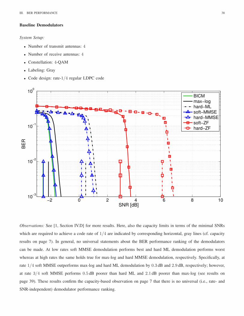
Baseline Demodulators
System Setup:
• Number of transmit antennas: 4
• Number of receive antennas: 4
• Constellation: 4-QAM
• Labeling: Gray
• Code design: rate-1/4 regular LDPC code
−2 0 2 4 6 8 1010
−3
10−2
10−1
100
SNR [dB]
BE
R
BICM
max−loghard−ML
soft−MMSE
hard−MMSEsoft−ZF
hard−ZF
Observations: See [1, Section IV.D] for more results. Here, also the capacity limits in terms of the minimal SNRs
which are required to achieve a code rate of 1/4 are indicated by corresponding horizontal, gray lines (cf. capacity
results on page 7). In general, no universal statements about the BER performance ranking of the demodulators
can be made. At low rates soft MMSE demodulation performs best and hard ML demodulation performs worst
whereas at high rates the same holds true for max-log and hard MMSE demodulation, respectively. Specifically, at
rate 1/4 soft MMSE outperforms max-log and hard ML demodulation by 0.3 dB and 2.9 dB, respectively; however,
at rate 3/4 soft MMSE performs 0.5 dB poorer than hard ML and 2.1 dB poorer than max-log (see results on
page 39). These results confirm the capacity-based observation on page 7 that there is no universal (i.e., rate- and
SNR-independent) demodulator performance ranking.

III. BER PERFORMANCE 39
Baseline Demodulators
System Setup:
• Number of transmit antennas: 4
• Number of receive antennas: 4
• Constellation: 4-QAM
• Labeling: Gray
• Code design: rate-3/4 regular LDPC code
6 8 10 12 14 16 1810
−3
10−2
10−1
100
SNR [dB]
BE
R
BICM
max−loghard−ML
soft−MMSE
hard−MMSEsoft−ZF
hard−ZF
Observations: See observations on page 38 and [1, Section IV.D] for more details. It is shown that whereas hard
ML demodulation performs poorer than soft MMSE demodulation at rate 1/4 (cf. page 38), for rate 3/4 its just
the other way round (by about 0.5 dB). This result agrees with the observations on page 7.

40
IV. IMPERFECT CHANNEL STATE INFORMATION AND NOISE VARIANCE
The following section investigates the ergodic system capacity for the case of imperfect channel state information
(CSI) at the receiver. In particular, we consider training-based estimation of the channel matrix H and the noise
variance σ2v . The transmitter sends Np > MT training vectors2 which are arranged into a full rank MT×Np training
matrix Xp. We assume that the transmit power per channel use for training and actual data is the same such that
the Frobenius norm [22] of Xp equals ‖Xp‖2F = NpEs. Assuming that the channel stays constant for the duration
of one block (which contains training and actual data), the MR × Np receive matrix Yp induced by the training is
given by (cf. (1))
Yp = HXp + V . (4)
Here, the MR × Np matrix V contains the noise received during the training period.
Using (4), the least-squares channel estimate (identical to the ML estimate under a Gaussian i.i.d. assumption for
the noise) is computed as [23]
H = YpXHp (XpX
Hp )−1 . (5)
The estimated channel matrix H is then used to obtain the noise variance estimate
σ2v =
1
MR(Np−MT)‖Yp − HXp‖
2F , (6)
which essentially amounts to measuring the mean power of Yp in the (Np−MT)-dimensional orthogonal complement
of the range space of XHp .
We consider the suboptimum generation of LLRs based on a mismatched demodulator metric (derived under the
perfect CSI assumption), i.e., we evaluate the demodulator outputs by replacing the perfect channel matrix and
noise variance in the corresponding metrics with its estimates.
In the following, we provide numerical results for the ergodic system capacity where we compare the case of
perfect and imperfect CSI. The latter assumes that both the channel and the noise variance are estimated using a
training-based ML estimator (cf. (5) and (6)) with the minimum number of Np = 5 pilot vectors. Throughout, a
4 × 4 MIMO system with 4-QAM and Gray labeling is considered (R0 = 8). For the baseline demodulators we
restrict to max-log, hard ML, and soft MMSE demodulation.
Furthermore, we analyze how the quality of the estimates influences the performance of the demodulators. Therefore,
we present a performance comparison in terms of the required minimum SNR to achieve a target code rate of
2 bpcu and 6 bpcu, respectively, over the amount of training vectors Np. For the baseline demodulators we consider
different variants which assume imperfect channel matrix (using (5)) and imperfect noise variance (using (6)),
imperfect channel matrix (using (5)) and perfect noise variance, and perfect channel matrix and imperfect noise
variance. For the latter case, the noise variance is estimated according to
σ2v =
1
MRNp
‖Yp − HXp‖2F ,
2While Np = MT is sufficient to estimate H, extra training is required for estimation of σ2
v .

IV. IMPERFECT CHANNEL STATE INFORMATION AND NOISE VARIANCE 41
(note that this equals the unbiased estimator for this case). As a reference, the results for perfect channel matrix
and perfect noise variance are indicated by corresponding horizontal, gray lines. For the remaining demodulators
we focus only on the case of imperfect channel and imperfect noise variance.
Additional observations and information about the system settings can be found in [1, Section VI].

IV. IMPERFECT CHANNEL STATE INFORMATION AND NOISE VARIANCE 42
Baseline Demodulators – Perfect vs. Imperfect CSI
System Setup:
• Number of transmit antennas: 4
• Number of receive antennas: 4
• Constellation: 4-QAM
• Labeling: Gray
• Number of pilot vectors for estimation: 5
−10 −5 0 5 10 15 200
1
2
3
4
5
6
7
8
Max. A
chie
vable
Rate
[bpcu
]
SNR [dB]
perfectimperfect
max−log
hard−ML
soft−MMSE
Observations: See results on page 44 and [1, Section VI] for more details. It is seen that for all three detectors
imperfect CSI results in a significant performance loss, e.g., at 4 bpcu the SNR loss for max-log, hard ML, and soft
MMSE is 3.9 dB, 3.2 dB, and 4 dB, respectively. In the considered worst case imperfect CSI setup the performance
advantage of soft MMSE demodulation over hard ML demodulation at low rates is a little bit less pronounced;
note that the cross-over between hard ML and soft MMSE performance shifts from 5.8 bpcu (at an SNR of about
7.7 dB) for perfect CSI to 5 bpcu (at 9.4 dB) for the case of imperfect CSI. However, the gap between soft MMSE
and max-log is slightly larger at low rates, e.g., 0.7 dB at 2 bpcu. The performance losses for all demodulators tend
to be smaller at high rates, which may be partly attributed to the fact that the CSI (in particular, the noise variance
estimate) becomes more accurate with increasing SNR. In general it can be observed that the performance loss of
hard ML is the smallest while soft MMSE and max-log performance deteriorates stronger; note that hard ML does
not use the noise variance and hence is more robust to estimation errors in σ2v . Here, hard ML comes within less

IV. IMPERFECT CHANNEL STATE INFORMATION AND NOISE VARIANCE 43
than 1.3 dB of max-log performance. In contrast, soft MMSE uses the imperfect channel and the noise variance
estimate in the MMSE equalization stage and in the LLR calculation and is thus most strongly affected.

IV. IMPERFECT CHANNEL STATE INFORMATION AND NOISE VARIANCE 44
Baseline Demodulators – Imperfect Channel/Imperfect Noise Variance
System Setup:
• Number of transmit antennas: 4
• Number of receive antennas: 4
• Constellation: 4-QAM
• Labeling: Gray
5 8 11 14 17 20−3
−2
−1
0
1
2
3
4
5
Required S
NR
[dB
]
Number of Pilots
2 bpcu max−log
hard−ML
soft−MMSE
5 8 11 14 17 206
7
8
9
10
11
12
136 bpcu
Re
qu
ire
d S
NR
[d
B]
Number of Pilots
max−log
hard−ML
soft−MMSE
Observations: See [1, Section VI] for more details. It is seen that for all demodulators, the required SNR decreases
rapidly with increasing amount of training. Yet, even for Np = 20 there is a significant gap of 1 to 2 dB to perfect
CSI performance. Here, soft MMSE consistently performs better than max-log and hard ML at 2 bpcu. Moreover,
it increases its SNR gap to hard ML by about 1 dB with a larger amount of training. In contrast, at 6 bpcu hard
ML outperforms soft MMSE, especially for very small training durations.

IV. IMPERFECT CHANNEL STATE INFORMATION AND NOISE VARIANCE 45
Baseline Demodulators – Imperfect Channel/Perfect Noise Variance
System Setup:
• Number of transmit antennas: 4
• Number of receive antennas: 4
• Constellation: 4-QAM
• Labeling: Gray
4 6 8 10 12 14 16 18 20
−2
0
2
4
6
Required S
NR
[dB
]
Number of Pilots
2 bpcu max−log
hard−ML
soft−MMSE
4 6 8 10 12 14 16 18 206
7
8
9
10
11
12
13
Re
qu
ire
d S
NR
[d
B]
Number of Pilots
6 bpcu max−log
hard−ML
soft−MMSE
Observations: Here, we assume that only the channel matrix is affected by imperfections due to channel estimation;
the noise variance is considered to be perfectly known at the receiver. The performance differences between the
demodulators are not as pronounced as in our worst case scenario (cf. page 44). The latter observations can be
explained by the fact that all demodulation techniques, that explicitly make use of the noise variance, may suffer from
further performance degradations if provided with very poor quality estimates of the noise variance. In particular,
this may affect the performance of all soft demodulation schemes, such as soft MMSE and max-log demodulation,
which require an accurate noise variance estimate for the LLR computation. However, the impact of the imperfect
noise variance on the demodulator performance is only very small (cf. also results on page 47). The differences lie

IV. IMPERFECT CHANNEL STATE INFORMATION AND NOISE VARIANCE 46
within 0.5 dB for the worst case of minimum training, i.e., Np = 5 pilots. Note that the performance of hard ML
demodulation essentially remains the same, since it does not require knowledge of the noise variance.

IV. IMPERFECT CHANNEL STATE INFORMATION AND NOISE VARIANCE 47
Baseline Demodulators – Perfect Channel/Imperfect Noise Variance
System Setup:
• Number of transmit antennas: 4
• Number of receive antennas: 4
• Constellation: 4-QAM
• Labeling: Gray
2 4 6 8 10 12 14 16 18 20−3
−2.5
−2
−1.5
−1
−0.5
0
0.5
Required S
NR
[dB
]
Number of Pilots
2 bpcu max−log
hard−ML
soft−MMSE
2 4 6 8 10 12 14 16 18 206
6.5
7
7.5
8
8.5
9
Required S
NR
[dB
]
Number of Pilots
6 bpcu max−log
hard−ML
soft−MMSE
Observations: It can be seen that the demodulator performance degrades if only a small amount of training pilots
is available to estimate the noise variance. However, the impact of the imperfect noise variance on the performance
is not very critical and lies within 0.5 dB even for very small amounts of training. Note that hard ML does not use
the noise variance and hence is more robust to estimation errors in σ2v . Using a sufficient amount of pilots, i.e.,
Np≥8, already closely approaches the performance obtained with perfect noise variance.

IV. IMPERFECT CHANNEL STATE INFORMATION AND NOISE VARIANCE 48
List Sphere Decoder (LSD) – Perfect vs. Imperfect CSI
System Setup:
• Number of transmit antennas: 4
• Number of receive antennas: 4
• Constellation: 4-QAM
• Labeling: Gray
• Number of pilot vectors for estimation: 5
−10 −5 0 5 10 150
1
2
3
4
5
6
7
8
SNR [dB]
Max. A
chie
vable
Rate
[bpcu
]
perfectimperfect
LSD−256/max−log
LSD−8
LSD−2
LSD−1/hard−ML
Observations: It can be seen that in this worst case scenario of imperfect channel and imperfect noise variance (Np =
5) changing the list size of the LSD no longer allows to go from hard ML to max-log performance (cf. page 17).
In fact, the LSD with list size |L|=8 slightly outperforms max-log demodulation; here, the latter equals the LSD
with a full candidate list (|L| = 256). We note that the usual performance tradeoff of the LSD can however be
experienced if more pilots for estimation are available at the receiver (cf. page 49).

IV. IMPERFECT CHANNEL STATE INFORMATION AND NOISE VARIANCE 49
List Sphere Decoder (LSD) – Imperfect Channel/Imperfect Noise Variance
System Setup:
• Number of transmit antennas: 4
• Number of receive antennas: 4
• Constellation: 4-QAM
• Labeling: Gray
5 8 11 14 17 20
−2
0
2
4
2 bpcu
Re
qu
ire
d S
NR
[d
B]
Number of Pilots
LSD−256/max−log
LSD−8
LSD−2
LSD−1/hard−ML
5 8 11 14 17 206
7
8
9
10
11 6 bpcu
Re
qu
ire
d S
NR
[d
B]
Number of Pilots
LSD−256/max−log
LSD−8
LSD−2
LSD−1/hard−ML
Observations: If only a small number of pilots is available for channel and noise variance estimation (Np =5), it
can be seen that the LSD with a list size of |L|=8 outperforms the LSD with full list (|L|=256). Although this is
not the case for larger training durations, LSD with |L| = 8 performs mostly very close to max-log for both rates.

IV. IMPERFECT CHANNEL STATE INFORMATION AND NOISE VARIANCE 50
Bit Flipping Demodulators (1-bit) – Perfect vs. Imperfect CSI
System Setup:
• Number of transmit antennas: 4
• Number of receive antennas: 4
• Constellation: 4-QAM
• Labeling: Gray
• Number of pilot vectors for estimation: 5
−10 −5 0 5 10 15 200
1
2
3
4
5
6
7
8
SNR [dB]
Ma
x.
Ach
ieva
ble
Ra
te [
bp
cu
]
perfectimperfect
max−log
flip−1,ML
hard−ML
flip−1,MMSE
Observations: It can be seen that the two bit flipping variants suffer from a severe performance degradation in
the case of imperfect CSI (Np = 5), i.e., a SNR shift of about 5 dB. The performance advantage of ML-based bit
flipping over pure hard ML demodulation is much smaller than in the case of perfect CSI; in fact, the SNR gap
lies only within 0.8 dB. Moreover, the performance cross-over between MMSE-based bit flipping demodulation and
hard ML demodulation shifts to lower rates, i.e., from 5.9 bpcu (at 7.8 dB) for perfect CSI to 4.9 bpcu (at 9.3 dB)
for imperfect CSI.

IV. IMPERFECT CHANNEL STATE INFORMATION AND NOISE VARIANCE 51
Bit Flipping Demodulators (1-bit) – Imperfect Channel/Imperfect Noise Variance
System Setup:
• Number of transmit antennas: 4
• Number of receive antennas: 4
• Constellation: 4-QAM
• Labeling: Gray
5 8 11 14 17 20
−2
0
2
4
2 bpcu
Re
qu
ire
d S
NR
[d
B]
Number of Pilots
max−log
flip−1,ML
hard−ML
flip−1,MMSE
5 8 11 14 17 206
7
8
9
10
11
126 bpcu
Re
qu
ire
d S
NR
[d
B]
Number of Pilots
max−log
flip−1,ML
hard−ML
flip−1,MMSE
Observations: At 2 bpcu, MMSE-based flipping slightly outperforms ML-based bit flipping by about 0.25 dB,
independent of the amount of training. At high rates and under imperfect CSI, the performance of MMSE-based
bit flipping is affected most of all. For example, at 6 bpcu and for Np = 5 the SNR gap to perfect CSI is 3.5 dB
for MMSE-based bit flipping whereas ML-based flipping reveals a gap of 3.1 dB.

IV. IMPERFECT CHANNEL STATE INFORMATION AND NOISE VARIANCE 52
Bit Flipping Demodulators (2-bit) – Perfect vs. Imperfect CSI
System Setup:
• Number of transmit antennas: 4
• Number of receive antennas: 4
• Constellation: 4-QAM
• Labeling: Gray
• Number of pilot vectors for estimation: 5
−10 −5 0 5 10 15 200
1
2
3
4
5
6
7
8
SNR [dB]
Ma
x.
Ach
ieva
ble
Ra
te [
bp
cu
]
perfectimperfect
max−log
flip−2,ML
hard−ML
flip−2,MMSE
Observations: Under imperfect CSI the performance of the MMSE-based bit flipping demodulator can be greatly
enhanced if the flipping is based on 2 bits instead of 1 bit. Except for an SNR shift, MMSE- and ML-based
flipping show the same performance behavior as for perfect CSI. MMSE-based bit flipping outperforms hard ML
demodulation and performs close to ML-based bit flipping and max-log demodulation at low-to-medium rates. Only
at very high rates it starts to perform poorer than hard ML demodulation.

IV. IMPERFECT CHANNEL STATE INFORMATION AND NOISE VARIANCE 53
Bit Flipping Demodulators (2-bit) – Imperfect Channel/Imperfect Noise Variance
System Setup:
• Number of transmit antennas: 4
• Number of receive antennas: 4
• Constellation: 4-QAM
• Labeling: Gray
5 8 11 14 17 20
−2
0
2
4
2 bpcu
Re
qu
ire
d S
NR
[d
B]
Number of Pilots
max−log
flip−2,ML
hard−ML
flip−2,MMSE
5 8 11 14 17 206
7
8
9
10
11 6 bpcu
Re
qu
ire
d S
NR
[d
B]
Number of Pilots
max−log
flip−2,ML
hard−ML
flip−2,MMSE
Observations: At 2 bpcu MMSE-based and ML-based bit flipping as well as max-log virtually show the same
performance, independent of the amount of training. At 6 bpcu the two flipping variants also show almost the same
performance for small training durations; however, when increasing the amount of training MMSE-based flipping
starts to slightly outperform ML-based flipping.

IV. IMPERFECT CHANNEL STATE INFORMATION AND NOISE VARIANCE 54
Lattice-Reduction-Aided Detector – Perfect vs. Imperfect CSI
System Setup:
• Number of transmit antennas: 4
• Number of receive antennas: 4
• Constellation: 4-QAM
• Labeling: Gray
• Number of pilot vectors for estimation: 5
−10 −5 0 5 10 15 200
1
2
3
4
5
6
7
8
SNR [dB]
Ma
x.
Ach
ieva
ble
Ra
te [
bp
cu
]
perfectimperfect
max−log
flip−1,LR−MMSE
hard−ML
hard−LR−MMSE
Observations: In comparison to the case of perfect CSI, hard and soft LR-based demodulation experience a
significant shift to higher SNRs under imperfect CSI estimation with minimum training length (Np =5). It can be
seen that at low rates the performance gaps between the hard and soft demodulators are reduced. The performance
cross-over between soft LR demodulation and hard ML demodulation shifts from 5.2 bpcu (at an SNR of about
6.7 dB) for the case of perfect CSI to 3.7 bpcu (at 7.6 dB) for imperfect CSI.

IV. IMPERFECT CHANNEL STATE INFORMATION AND NOISE VARIANCE 55
Lattice-Reduction-Aided – Imperfect Channel/Imperfect Noise Variance
System Setup:
• Number of transmit antennas: 4
• Number of receive antennas: 4
• Constellation: 4-QAM
• Labeling: Gray
5 8 11 14 17 20
−2
0
2
4
62 bpcu
Re
qu
ire
d S
NR
[d
B]
Number of Pilots
max−log
flip−1,LR−MMSE
hard−ML
hard−LR−MMSE
5 8 11 14 17 206
8
10
12
146 bpcu
Re
qu
ire
d S
NR
[d
B]
Number of Pilots
max−log
flip−1,LR−MMSE
hard−ML
hard−LR−MMSE
Observations: At 2 bpcu it can be seen that hard ML slightly outperforms hard LR demodulation for small training
durations; however, for Np > 10 it is the other way around. At 6 bpcu all the demodulators show the same SNR
gap of about 3 dB which decreases consistently with increasing amount of training.

IV. IMPERFECT CHANNEL STATE INFORMATION AND NOISE VARIANCE 56
Semidefinite Relaxation (SDR) Detector – Perfect vs. Imperfect CSI
System Setup:
• Number of transmit antennas: 4
• Number of receive antennas: 4
• Constellation: 4-QAM
• Labeling: Gray
• Number of pilot vectors for estimation: 5
−10 −5 0 5 10 15 200
1
2
3
4
5
6
7
8
SNR [dB]
Ma
x.
Ach
ieva
ble
Ra
te [
bp
cu
]
perfectimperfect
max−log
soft−SDR
hard−ML
hard−SDR
Observations: Similarly as for the perfect CSI case, hard and soft SDR demodulation also exactly coincide with
hard ML and max-log performance in the case of imperfect CSI. This behavior is independent of the amount of
training, as shown on page 57. However, the gap between hard and soft demodulation reduces by about 1 dB for
the worst-case scenario of minimum training length (Np≤5).

IV. IMPERFECT CHANNEL STATE INFORMATION AND NOISE VARIANCE 57
Semidefinite Relaxation (SDR) Detector – Imperfect Channel/Imperfect Noise Variance
System Setup:
• Number of transmit antennas: 4
• Number of receive antennas: 4
• Constellation: 4-QAM
• Labeling: Gray
5 8 11 14 17 20−3
−2
−1
0
1
2
3
4
52 bpcu
Re
qu
ire
d S
NR
[d
B]
Number of Pilots
max−log
soft−SDR
hard−ML
hard−SDR
5 8 11 14 17 206
7
8
9
10
11 6 bpcu
Re
qu
ire
d S
NR
[d
B]
Number of Pilots
max−log
soft−SDR
hard−ML
hard−SDR
Observations: Even in the case of imperfect CSI hard and soft SDR demodulation match the performance of hard
ML and max-log demodulation. This behavior is independent of the amount of training. The gap between hard and
soft demodulation increases by about 1 dB when increasing the amount of training.

IV. IMPERFECT CHANNEL STATE INFORMATION AND NOISE VARIANCE 58
ℓ∞-Norm Demodulator – Perfect vs. Imperfect CSI
System Setup:
• Number of transmit antennas: 4
• Number of receive antennas: 4
• Constellation: 4-QAM
• Labeling: Gray
• Number of pilot vectors for estimation: 5
−10 −5 0 5 10 15 200
1
2
3
4
5
6
7
8
SNR [dB]
Ma
x.
Ach
ieva
ble
Ra
te [
bp
cu
]
perfectimperfect
max−log
soft−Linf
hard−ML
hard−Linf
Observations: The main observation in this worst-case scenario (Np = 5) is that the performance gaps between
max-log, soft ℓ∞-norm, hard ML, and hard ℓ∞-norm demodulation are significantly reduced. In general, soft ℓ∞-
norm demodulation appears to be more sensitive to poor quality estimates of the channel and the noise variance
than hard ℓ∞-norm demodulation (cf. page 59).

IV. IMPERFECT CHANNEL STATE INFORMATION AND NOISE VARIANCE 59
ℓ∞-Norm Demodulator – Imperfect Channel/Imperfect Noise Variance
System Setup:
• Number of transmit antennas: 4
• Number of receive antennas: 4
• Constellation: 4-QAM
• Labeling: Gray
5 8 11 14 17 20
−2
0
2
4
62 bpcu
Re
qu
ire
d S
NR
[d
B]
Number of Pilots
max−log
soft−Linf
hard−ML
hard−Linf
5 8 11 14 17 206
7
8
9
10
11
12 6 bpcu
Re
qu
ire
d S
NR
[d
B]
Number of Pilots
max−log
soft−Linf
hard−ML
hard−Linf
Observations: In general, soft ℓ∞-norm demodulation appears to be more sensitive to poor quality estimates of
the channel and the noise variance than hard ℓ∞-norm demodulation. For example, at 2 bpcu and for Np = 5 the
performance gap to perfect CSI equals 4.23 dB. In contrast, hard ℓ∞-norm demodulation is more robust, showing
only a gap of 3.2 dB in this case.

IV. IMPERFECT CHANNEL STATE INFORMATION AND NOISE VARIANCE 60
Successive Interference Canceler (SIC) and Soft Interference Canceler (SoftIC) – Perfect vs. Imperfect CSI
System Setup:
• Number of transmit antennas: 4
• Number of receive antennas: 4
• Constellation: 4-QAM
• Labeling: Gray
• Number of pilot vectors for estimation: 5
−10 −5 0 5 10 15 200
1
2
3
4
5
6
7
8
SNR [dB]
Ma
x.
Ach
ieva
ble
Ra
te [
bp
cu
]
perfectimperfect
SoftIC
max−log
hard−ML
MMSE−SIC
Observations: With imperfect CSI, the performance curves of SoftIC demodulation (with 3 iterations and initial-
ized with soft ZF) experience a significant shift to lower SNRs. In comparison to hard ML demodulation, the
performance of SoftIC demodulation suffers from a stronger degradation; the cross-over between SoftIC and hard
ML demodulation shifts from 6.3 bpcu to 4.3 bpcu at an SNR of about 8.5 dB. The performance gap between
MMSE-SIC and max-log demodulation reduces for the case of imperfect CSI by about 1 dB. Although, in general,
MMSE-SIC demodulation has inferior performance than SoftIC at low rates, it remains more robust for the case
of imperfect CSI.

IV. IMPERFECT CHANNEL STATE INFORMATION AND NOISE VARIANCE 61
Successive Interference Canceler (SIC) and Soft Interference Canceler (SoftIC) – Imperfect Channel/Imperfect
Noise Variance
System Setup:
• Number of transmit antennas: 4
• Number of receive antennas: 4
• Constellation: 4-QAM
• Labeling: Gray
5 8 11 14 17 20
−2
0
2
4
62 bpcu
Re
qu
ire
d S
NR
[d
B]
Number of Pilots
SoftIC
max−log
hard−ML
MMSE−SIC
5 8 11 14 17 206
8
10
12
146 bpcu
Re
qu
ire
d S
NR
[d
B]
Number of Pilots
SoftIC
max−log
hard−ML
MMSE−SIC
Observations: Although, in general, MMSE-SIC demodulation has inferior performance than SoftIC at low rates,
it remains more robust for the case of imperfect CSI; for example, at 2 bpcu MMSE-SIC shows a performance gap
to perfect estimation of 4 dB for Np =5 whereas SoftIC demodulation has a gap of 5.2 dB in this case. The inferior
robustness of SoftIC over MMSE-SIC can also be seen at high rates (6 bpcu) where the performance degradation
of SoftIC is more pronounced for the case of small training durations.

62
V. QUASI-STATIC FADING
In this section we provide a demodulator performance comparison for the i.i.d. quasi-static fading MIMO channel.
In this case the channel H is random but constant over time, i.e., each codeword can extend over only one channel
realization [24]. Since in this regime, an ergodic system capacity of the equivalent modulation channel is no longer
meaningful [24], [25], we consider the outage probability
Pout(R) , P{RH<R}, (7)
where RH is a random variable defined as
RH ,
R0∑
l=1
IH(cl; Λl).
Here, IH(cl; Λl) denotes the conditional mutual information given a fixed channel realization (cf. (2)). Note that
the ergodic system capacity C in (2) equals C = EH{RH}. The outage probability Pout(R) can be interpreted as
the smallest probability of error achievable at rate R [25]. A closely related concept is given by the ǫ-capacity of
the equivalent modulation channel, defined as [25]
Cǫ , sup {R | P{RH<R} < ǫ} . (8)
The ǫ-capacity may be interpreted as the maximum rate for which a probability of error less than ǫ can be achieved.
We refer to [1, Section III.D] for more details on these measures.
In our discussion we focus on the baseline demodulators (reviewed in [1, Section IV.A]) and investigate a 4×4
MIMO system with 4-QAM employing Gray labeling. We first show the outage probability in (7) versus SNR for a
target rates of R = 2 bpcu and R = 6 bpcu. The outage probability Pout(R) was measured using 105 blocks (affected
by independent fading realizations), each consisting of 105 symbol vectors. Furthermore, we plot the ǫ-capacity
in (8) over SNR for a maximum outage probability of ǫ = 10−2 and note that these results are qualitatively very
similar to the results obtained for the ergodic capacity on page 7.
Additional observations can be also found in [1, Section VII].

V. QUASI-STATIC FADING 63
Baseline Demodulators
System Setup:
• Number of transmit antennas: 4
• Number of receive antennas: 4
• Constellation: 4-QAM
• Labeling: Gray
−10 −5 0 5 10 15 20 25 3010
−3
10−2
10−1
100
SNR [dB]
Ou
tag
e P
rob
ab
ility
2 bpcu 6 bpcu
BICM
max−loghard−ML
soft−MMSE
hard−MMSEsoft−ZF
hard−ZF
Observations: See [1, Section VII] for more details. For R=2 bpcu, it is seen that optimum soft MAP demodulation
(labeled ‘BICM’ for consistency with previous sections) and soft MMSE demodulation exactly coincide and show
a gap to max-log demodulation of about 0.5 dB. In such a low-rate regime, max-log performs about 2.5 dB better
than hard ML. While max-log, hard ML, and soft MMSE demodulation all achieve full diversity (cf. the slope of
the corresponding outage probability curves), soft and hard ZF only have diversity order one, resulting in a huge
performance loss (almost 19 dB and 20.5 dB at Pout(R) = 10−2, respectively). At R=6 bpcu the situation is quite
different: here, max-log coincides with soft MAP and hard ML looses only 1.4 dB (again, those three demodulators
achieve full diversity). Surprisingly, hard and soft MMSE deteriorate at this rate, starting to loose all diversity. At
Pout(R) = 10−2, the SNR loss of soft MMSE and soft ZF relative to max-log equals about 4.4 dB and 19 dB,
respectively.

V. QUASI-STATIC FADING 64
Baseline Demodulators
System Setup:
• Number of transmit antennas: 4
• Number of receive antennas: 4
• Constellation: 4-QAM
• Labeling: Gray
• Fixed maximum outage probability: ǫ = 10−2
−10 −5 0 5 10 15 20 25 30 350
1
2
3
4
5
6
7
8
Ma
x. ε−
Ach
ieva
ble
Ra
te
SNR [dB]
BICM
max−loghard−ML
soft−MMSE
hard−MMSEsoft−ZF
hard−ZF
Observations: See [1, Section VII] for more details. Some of the behavior of the ǫ-capacity curves is qualitatively
very similar to the results obtained for the ergodic capacity on page 7: at low rates soft MMSE demodulation
outperforms hard ML demodulation (by up to 2.8 dB for rates less than 4.7 bpcu) while at high rates it is the
other way round. Furthermore, for low rates soft MMSE demodulation essentially coincides with optimum soft
MAP demodulation whereas at high rates it approaches soft ZF performance. We note that a similar rate-dependent
diversity behavior of MMSE demodulation has been observed in [26]. In particular, the authors proved that in case
of joint spatial encoding the upper bound on the outage probability of hard MMSE receivers decays with diversity
order of MTMR at low rates and decays with order MR − MT + 1 at high rates; in contrast, hard ZF always has
diversity no better than MR −MT + 1. This very well fits with our observations where the MMSE demodulator is
seen to loose all its diversity for rates larger than 5 bpcu.
A comparison of these results with the ergodic results on page 7 even suggests that there is a connection between

V. QUASI-STATIC FADING 65
the diversity of the demodulators in the quasi-static scenario and their SNR gap to optimum demodulation in the
ergodic scenario. For all rates (and all SNRs), the max-log and hard ML demodulator both achieve constant (full)
diversity in the quasi-static regime and maintain a roughly constant gap to soft MAP in the ergodic scenario. On
the other hand, the diversity of soft and hard MMSE demodulation in the quasi-static case and their SNR gaps to
soft MAP in the ergodic scenario both deteriorate with increasing rate/SNR. Note that also here hard and soft ZF
demodulation perform worst, with a diversity equal to 1 for all rates.

66
REFERENCES
[1] P. Fertl, J. Jalden, and G. Matz, “Performance assessment of MIMO-BICM demodulators based on system capacity,” Oct. 2009,
submitted to IEEE Trans. Signal Processing.
[2] G. Caire, G. Taricco, and E. Biglieri, “Bit-interleaved coded modulation,” IEEE Trans. Inf. Theory, vol. 44, no. 5, pp. 927–945, May
1998.
[3] S. H. Muller-Weinfurtner, “Coding approaches for multiple antenna transmission in fast fading and OFDM,” IEEE Trans. Signal
Processing, vol. 50, no. 10, pp. 2442–2450, Oct. 2002.
[4] A. Guillen i Fabregas, A. Martinez, and G. Caire, “Bit-Interleaved Coded Modulation,” Foundations and Trends in Communications
and Information Theory, vol. 5, no. 1–2, pp. 1–153, 2008.
[5] T. J. Richardson and R. L. Urbanke, “The capacity of low-density parity check codes under message-passing decoding,” IEEE Trans.
Inf. Theory, vol. 47, no. 2, pp. 599–618, Feb. 2001.
[6] A. Paulraj, R. U. Nabar, and D. Gore, Introduction to Space-Time Wireless Communications. Cambridge (UK): Cambridge Univ.
Press, 2003.
[7] M. R. McKay and I. B. Collings, “Capacity and performance of MIMO-BICM with zero-forcing receivers,” IEEE Trans. Comm.,
vol. 53, no. 1, pp. 74–83, Jan. 2005.
[8] D. Seethaler, G. Matz, and F. Hlawatsch, “An efficient MMSE-based demodulator for MIMO bit-interleaved coded modulation,” in
Proc. IEEE GLOBECOM-2004, vol. 4, Dallas, Texas, Dec. 2004, pp. 2455–2459.
[9] B. M. Hochwald and S. ten Brink, “Achieving near-capacity on a multiple-antenna channel,” IEEE Trans. Inf. Theory, vol. 51, no. 3,
pp. 389–399, Mar. 2003.
[10] R. Wang and G. B. Giannakis, “Approaching MIMO channel capacity with soft detection based on hard sphere decoding,” IEEE Trans.
Comm., vol. 54, no. 4, pp. 587–590, Apr. 2006.
[11] D. Wubben, R. Bohnke, V. Kuhn, and K. Kammeyer, “MMSE-based lattice-reduction for near-ML detection of MIMO systems,” in
Proc. ITG Workshop on Smart Antennas 2004, Munich, Germany, Mar. 2004, pp. 106–113.
[12] B. Steingrimsson, Z.-Q. Luo, and K. M. Wong, “Soft quasi-maximum-likelihood detection for multiple-antenna wireless channels,”
IEEE Trans. Signal Processing, vol. 51, no. 11, pp. 2710–2719, Nov. 2003.
[13] A. Burg, M. Borgmann, M. Wenk, M. Zellweger, W. Fichtner, and H. Bolcskei, “VLSI implementation of MIMO detection using sphere
decoding algorithm,” IEEE J. Solid-State Circuits, vol. 40, no. 7, pp. 1566–1577, July 2005.
[14] D. Seethaler and H. Bolcskei, “Infinity-norm sphere-decoding,” in IEEE Int. Symposium on Information Theory (ISIT), Toronto, Canada,
July 2008, pp. 2002–2006.
[15] R. Bohnke, D. Wubben, V. Kuhn, and K. D. Kammeyer, “Reduced complexity MMSE detection for BLAST architectures,” in Proc.
IEEE GLOBECOM-2003, vol. 4, San Francisco, CA, Dec. 2003, pp. 2258–2262.
[16] W.-J. Choi, K.-W. Cheong, and J. Cioffi, “Iterative soft interference cancellation for multiple antenna systems,” in Proc. IEEE WCNC-
2000, vol. 1, Chicago, IL, Sep. 2000, pp. 304–309.
[17] C. Studer and H. Bolcskei, “Soft-input soft-output single tree-search sphere decoding,” IEEE Trans. Inf. Theory, vol. 56, no. 10, pp.
4827–4842, Oct. 2010.
[18] M. van Dijk, A. J. E. M. Janssen, and A. G. C. Koppelaar, “Correcting systematic mismatches in computed log-likelihood ratios,”
Europ. Trans. Telecomm., vol. 14, no. 3, pp. 227–244, July 2003.
[19] A. Burg, M. Wenk, and W. Fichtner, “VLSI implementation of pipelined sphere decoding with early termination,” in Proc. EUSIPCO-
2006, Florence, Italy, Sept. 2006.
[20] S. Schwandter, P. Fertl, C. Novak, and G. Matz, “Log-likelihood ratio clipping in MIMO-BICM systems: Information geometric analysis
and impact on system capacity,” in Proc. IEEE ICASSP-2009, Taipei, Taiwan, Apr. 2009, pp. 2433–2436.
[21] C. Novak, P. Fertl, and G. Matz, “Quantization for soft-output demodulators in bit-interleaved coded modulation systems,” in Proc.
IEEE ISIT-2009, Seoul, Korea, Jun./Jul. 2009, pp. 1070–1074.
[22] R. A. Horn and C. R. Johnson, Matrix Analysis. Cambridge (UK): Cambridge Univ. Press, 1999.
[23] M. Biguesh and A. B. Gershman, “Training-based MIMO channel estimation: A study of estimator tradeoffs and optimal training
signals,” IEEE Trans. Signal Processing, vol. 54, no. 3, pp. 884–893, Mar. 2006.
[24] D. Tse and P. Viswanath, Fundamentals of Wireless Communication. Boston (MA): Cambridge University Press, 2005.
[25] A. Lapidoth and P. Naryan, “Reliable communication under channel uncertainty,” IEEE Trans. Inf. Theory, vol. 44, no. 6, pp. 2148–2177,
Oct. 1998.
[26] A. Hedayat and A. Nosratinia, “Outage and diversity of linear receivers in flat-fading MIMO channels,” IEEE Trans. Signal Processing,
vol. 55, no. 12, pp. 5868–5873, Dec. 2007.