performance assessment of different data mining methods in statistical downscaling of daily...
TRANSCRIPT

Accepted Manuscript
Performance Assessment of Different Data Mining Methods in Statistical
Downscaling of Daily Precipitation
M. Nasseri, H. Tavakol-Davani, B. Zahraie
PII: S0022-1694(13)00300-4
DOI: http://dx.doi.org/10.1016/j.jhydrol.2013.04.017
Reference: HYDROL 18844
To appear in: Journal of Hydrology
Received Date: 16 April 2012
Revised Date: 7 April 2013
Accepted Date: 9 April 2013
Please cite this article as: Nasseri, M., Tavakol-Davani, H., Zahraie, B., Performance Assessment of Different Data
Mining Methods in Statistical Downscaling of Daily Precipitation, Journal of Hydrology (2013), doi: http://
dx.doi.org/10.1016/j.jhydrol.2013.04.017
This is a PDF file of an unedited manuscript that has been accepted for publication. As a service to our customers
we are providing this early version of the manuscript. The manuscript will undergo copyediting, typesetting, and
review of the resulting proof before it is published in its final form. Please note that during the production process
errors may be discovered which could affect the content, and all legal disclaimers that apply to the journal pertain.

1
Performance Assessment of Different Data Mining 1
Methods in Statistical Downscaling of Daily Precipitation 2
M. Nasseri1, H. Tavakol-Davani2, B. Zahraie3 3
Abstract 4
In this paper, nonlinear Data-Mining (DM) methods have been used to extend the most cited 5
statistical downscaling model, SDSM, for downscaling of daily precipitation. The proposed 6
model is Nonlinear Data-Mining Downscaling Model (NDMDM). The four nonlinear and 7
semi-nonlinear DM methods which are included in NDMDM model are cubic-order 8
Multivariate Adaptive Regression Splines (MARS), Model Tree (MT), k-Nearest Neighbor 9
(kNN) and Genetic Algorithm-optimized Support Vector Machine (GA-SVM). The daily 10
records of 12 rain gauge stations scattered in basins with various climates in Iran are used to 11
compare the performance of NDMDM model with statistical downscaling method. 12
Comparison between statistical downscaling and NDMDM results in the selected stations 13
indicates that combination of MT and MARS methods can provide daily rain estimations 14
with less mean absolute error and closer monthly standard deviation and skewness values to 15
the historical records for both calibration and validation periods. The results of the future 16
projections of precipitation in the selected rain gauge stations using A2 and B2 SRES 17
scenarios show significant uncertainty of the NDMDM and statistical downscaling models. 18
19
Key Words: Statistical Downscaling, nonlinear Data-Mining method, Climate Change, 20
21
1
Ph.D. Candidate, School of Civil Engineering, University of Tehran, Tehran, Iran, Corresponding Author,
Graduate Student, School of Civil Engineering, University of Tehran, Tehran, Iran, [email protected], 3
Associate Professor, Center of Excellence for Engineering and Management of Civil Infrastructures, School of
Civil Engineering, University of Tehran, Tehran, Iran, [email protected], P.O. Box 11155-4563

2
1. Introduction 22
Outputs of Global Circulation Models (GCMs) are the base of climate change studies. 23
Spatial resolution of these data is not enough to determine local climate change effects and 24
they must be recalculated to a suitable resolution to be valid for local meteorological analysis. 25
The methods of extracting regional scale meteorological variables from GCM outputs have 26
been known as downscaling approaches. Four general categories of downscaling approaches 27
include regression (empirical) methods (Enke and Spekat, 1997; Faucher et al. 1999; Li and 28
Sailor, 2000; Wilby et al. 2002; Hessami et al. 2008; Raje and Mujumdar, 2011), weather 29
pattern approaches (Bárdossy and Plate, 1992; Yarnal et al. 2001; Bárdossy et al. 2002; 30
Wetterhall et al., 2009; Anandhi et al. 2011), stochastic weather generators (Semenov and 31
Barrow, 1997; Bates et al. 1998) and regional climate models (Mearns et al. 1995). 32
Regression or empirical methods are the most cited approaches in downscaling 33
simulation. Simplicity in use, relatively lower costs of pre-processing and straightforwardness 34
of computational procedure are the main reasons of the popularity of these downscaling 35
techniques. 36
Finding the empirical relationships between global and local scales of climate circulation 37
is the basic statement of any statistical downscaling method. According to this assumption, 38
correlation of global GCM meteorological variables (predictors) and local meteorological 39
variables such as observed precipitation and temperature (predictands) is the key point of this 40
type of downscaling procedure. The most well-known regression based downscaling methods 41
are structured for separate estimation of occurrence and amount of meteorological variables. 42
Advantages and disadvantages of statistical regression based downscaling methods have been 43
comprehensively discussed by Hessami et al. (2008). 44
Different nonlinear Data Mining (DM) methods such as Artificial Neural Networks 45
(ANN) (Tomassetti et al. 2009; Pasini, 2009; Mendes and Marengo, 2010; Fistikoglu and 46

3
Okan, 2011), k-Nearest Neighbor (kNN) (Yates et al. 2003; Gangopadhyay et al. 2005; Raje 47
and Mujumdar, 2011), Support Vector Machine (SVM) (Tripathi et al. 2006; Chen et al. 48
2010), Model Tree (MT) (Li and Sailor 2000), Multivariate Adaptive Regression Splines 49
(MARS) (Corte-Real et al. 1995) beside linear regression methods (Wilby et al. 2002; 50
Hessami et al. 2008) have been used in the previous studies for climatological research. 51
SDSM (Statistical DownScaling Model) is the most cited concepts and packages among 52
regression based statistical downscaling methods. This computer package benefits from 53
Multiple Linear Regression (MLR) method to estimate the amount and/or the occurrence of 54
local meteorological predictands. 55
In this paper, efficiency of four nonlinear and semi-nonlinear DM methods and their 56
previous applications in climatological research, namely MARS, MT, kNN and Genetic 57
Algorithm-optimized SVM (GA-SVM) have been evaluated versus application of the 58
standard MLR in estimating both occurrence and amount of precipitation. In this article, the 59
structure of SDSM has been used as the main platform to develop Nonlinear Data-Mining 60
Downscaling Model (NDMDM) model by replacing their MLR kernels with the selected DM 61
methods. In the next sections, local scale (areas of interest and predictands) and large scale 62
datasets (predictors) which are used in this study are described. Then, SDSM and the utilized 63
DM methods are briefly described. The next sections of the paper present the results of the 64
case study and concluding remarks and recommendations for further studies. 65
66
2. Datasets 67
2.1. Local Dataset 68
To assess the efficiency of the proposed downscaling method, twelve rain gauge stations 69
scattered in five different climatological basins in Iran, namely Hamoon-Jazmoorian, 70
Sefidrood, Mordab-Anzali, Shapoor-dalky and Mond are used. These basins are located in an 71

4
arid region in southeast of Iran near Iran-Pakistan border, a wet region in north of Iran near 72
Caspian Sea and a semi-arid region in southwest of Iran in Persian Gulf. Some statistical 73
characteristics such as average, maximum and standard deviation of observed daily 74
precipitation of the selected stations have been presented in Table 1. The locations of these 75
rain gauge stations are also shown in Fig. 1. As presented in Table 1, twenty six to thirty five 76
years of daily precipitation records up to the year 2000 (the start year of simulations of the 77
climate change scenarios) are available for the selected rain gauge stations. For each station, 78
the first 75% of the available record has been used for calibration of the downscaling model 79
and the rest of the recorded data has been used for validation of the model. The daily 80
precipitation records have been gathered from the Iran Water Resources Management 81
Company. 82
83
2.2. Large scale Datasets 84
The data bank of Hadley Center GCM, namely HadCM3, for A2 and B2 SRES (Special 85
Report on Emission Scenarios) scenarios has been used in this study to project the future 86
climate behavior. The coarse resolution (2.5° × 2.5°) reanalysis of atmospheric data from the 87
U.S. National Center for Environmental Prediction (NCEP) (Table 2) have been used as the 88
downscaling model predictors. 89
Because of inconsistency of spatial resolution of HadCM3 outputs (3.75° (long.) × 2.5° 90
(lat.)) and NCEP dataset, projection of large-scale predictors of NCEP on HadCM3 91
computational grid box has been used in this study. The daily projected data and HadCM3 92
outputs are available from the Canadian Climate Impacts Scenarios (CCIS) website 93
(www.cics.uvic.ca/scenarios/sdsm/select.cgi). 94
Twenty six different atmospheric variables are available for each grid box in this 95
database. For each rain gauge station, nine boxes covering and around the study areas have 96

5
been selected. Fig. 1 depicts center of each meteorological grid box and location of the 97
selected rain gauge stations. As it is illustrated in this figure, the grid boxes cover a large area 98
over the selected basins and around them. In addition, one to three-day lags of predictors 99
have been considered as candidate model inputs to incorporate cross correlation and auto-100
correlation in the modeling process. For each station, 936 (9 (grid boxes) × 26 101
(meteorological predictors) ×4 (0 to 3-day time lag)) predictors have been analyzed. 102
103
3. Methodology 104
In the current section at the first, platform of SDSM has been described. Then different 105
data-mining methods which are used in NDMDM are described and at the end, structure of 106
NDMDM is explained. 107
108
3.1. Statistical DownScaling Model (SDSM) 109
SDSM software is developed based on Multiple Linear Regression Downscaling Model 110
(MLRDM) (Wilby et al. 2002). SDSM outputs are the average of several weather ensembles 111
which are the results of using linear regression models with stochastic terms of bias 112
correction. Because of the linear structure of SDSM, selection of predictors is based on the 113
correlation and partial correlation analysis between the predictand and predictors and weights 114
of the predictors which are estimated via simple least square method. Dual simplex method 115
has been also provided in SDSM because of instability of regression coefficients for non-116
orthogonal predictor vectors. Hessami et al. (2008) added a new option of using ridge 117
regression (Hoerl and Kennard, 1970) in their downscaling model, namely ASD as a remedy 118
of the non-orthogonality impact of the predictor vectors as well (Hessami et al. 2008). 119
SDSM model contains of two separate sub-models to determine occurrence and amount 120
of conditional meteorological variables (or discrete variables) such as precipitation and 121

6
amount model for unconditional variables (or continues variables) such as temperature or 122
evaporation. Statistical downscaling using SDSM consists of the following steps: 123
1. In first step, suitable predictors should be selected. SDSM provides the ability of 124
some statistical analysis for users to select the best predictors. In SDSM, predictors 125
should have acceptable unconditional and conditional correlations with the 126
predictand. Also, partial correlation, P-Value and explained variance of the predictors 127
can be checked while using SDSM. The scatter plot is another tool provided in SDSM 128
in order to select the appropriate predictors. Acceptable ranges for the above 129
mentioned terms are proposed by Wilby et al. (2004). 130
2. A multiple linear regression model is calibrated to simulate the precipitation 131
occurrence which is called unconditional model. This model can be calibrated by two 132
different methods namely ordinary least square and dual simplex methods. An 133
autoregressive term can be added to this model. For each month, one MLR model 134
must be calibrated for occurrence estimation. The days with and without events 135
(precipitation) are represented with 1 and 0, respectively. For each day and ensemble, 136
a uniformly distributed random number between 0 and 1 is generated. If the random 137
number is less than the output of the occurrence model in that day, precipitation 138
occurs. Otherwise, precipitation does not occur. 139
3. Another multiple linear regression model, namely conditional model, is calibrated to 140
simulate the precipitation amount. This model is calibrated using the rainy days data. 141
Like the unconditional model, SDSM calibrate different conditional models for 12 142
months of year. For a day which is identified as a rainy day in the previous step, 143
output of the amount model is calculated. Then, a normally distributed number is 144
added to the output to consider the modeling error. This random number is generated 145
7
using a normal distribution function with zero mean and standard deviation equal to 146
standard error. 147
4. The result of the previous step is compared with a pre-defined threshold. If the result 148
is less than the threshold, the precipitation won’t occur. Otherwise, the result is 149
considered as the rainfall amount in that day and in that ensemble. 150
5. Furthermore, in SDSM, bias correction (b) (Eq. 1) and variance inflation (VIF) (Eq. 151
2) actions can be applied on the results of each monthly model to achieve acceptable 152
ensemble results both in the calibration and validation periods (Hessami et al. 2008): 153
modMeanMeanb obs (1)
2
12
Ste
VarVarVIF obs )( mod
(2)
Where Meanobs and Meanmod are the mean values of the observed and modeled 154
precipitation, respectively. Varobs and Varmod are the variances of observed and 155
modeled precipitation for the calibration period and Ste is the standard error in the 156
same period. b-1 is added to the amount of precipitation in each day and 12
VIF is 157
multiplied to the standard deviation of modeling error. While the downscaling model 158
is calibrated using NCEP dataset, in estimating VIF and bias correction, variables with 159
the subscript Mod are estimated using downscaling model outputs based on GCM 160
simulations. This approach allows the modeler to take into account the bias of GCM 161
in the downscaling process. 162
6. Finally, in order to achieve a single downscaled time series from all projected 163
ensembles, their arithmetic mean are calculated. 164
In this study, SDSM has been rewritten in MATLAB environment. Accuracy and 165
compatibility of the new MATLAB code with SDSM package has been tested using several 166
datasets. Then the SDSM MATLAB code has been extended to make the user capable of 167

8
choosing different predictors for the amount and occurrence models. Because of this 168
difference between the commercial SDSM package developed by Wilby et al. (2002) and the 169
code developed in this study, we have referred to it as MLRDM in the next sections of the 170
paper. 171
172
3.2. MARS 173
Initial idea of MARS (Friedman and Stueltze, 1981) has been developed and completed 174
by Friedman (1991). This method is based on multivariate regression with linear or nonlinear 175
mathematical kernels enhanced by continuous data partitioning. Various applications of 176
MARS can be found in hydrological studies (Coulibaly and Bladwin, 2005; Buccola and 177
Wood, 2010; Herrera et al. 2010). MARS detects inherent data nonlinearity and appropriate 178
partitions of data structure for model parameters using weighted summation of some 179
conditional linear or nonlinear polynomial basis functions. MARS uses the following 180
structure for conditional regression: 181
k
i
ii xBCxf1
)()( (3)
Where, )(xBi and iC are the basis function and its constant coefficient, respectively and 182
also k is the number of total basis functions used in the final model. Basis functions are 183
known as hinge function. The general form of hinge functions is as follows: 184
),0max(),0max()( iiiii xconstorconstxxB (4)
In Eq. 4, hinge function is linear while it is also possible to be presented in the form of 185
multiple nonlinear functions with orders higher than one. MARS has two important backward 186
and forward routines for identifying the best structure and especially the model parameters. 187
These coupled routines allow optimization of the MARS structure avoiding over 188
9
parameterization and over-fitting effects. For more information, the readers are referred to 189
Friedman and Stueltze (1981). 190
FAST MARS (Friedman, 1993), ARESLab (Jekabsons, 2010) are the recent softwares 191
developed for MARS. The ARESLab package provided by Jekabsons (2010) has been 192
utilized in this study, and maximum order of polynomial function in ARESLab has been set 193
up to 3. 194
195
3.3. Model Tree (MT) 196
MT is classified as a data-structured and modular DM method. Similar to MARS, MT is 197
also built on a data partitioning foundation. MT splits rules at the leaves of the conceptual 198
mathematical tree in non-terminal nodes of regression functions. So, the construction of a MT 199
is similar to that of decision tree while it has faster convergence compared with other DM 200
methods. MT can successfully manage problems with high dimensional spaces up to 201
hundreds of variables, and also combines a conventional model tree with the possibility of 202
generating linear regression functions at its leaves through increasing simulation 203
performance. MT operates very similar to piecewise or conditional mathematical functions. 204
One of the first applications of conditional regression method to describe behavior of 205
hydrological rainfall-runoff system has been presented in the 1970s by Becker (1976) and 206
also with Becker and Kundzewicz (1987). MT has found many applications in climatological 207
and hydrological sciences (Faucher et al. 1999; Li and Sailor, 2000; Xiong et al. 2001; 208
Solomatine and Xue, 2004). 209
M5 is a popular MT method. M5 learning paradigm was developed by Quinlan (1986, 210
1993). The first version of M5 consisted of piecewise or conditional linear models, which 211
made it an intermediate model between the linear models and truly nonlinear models such as 212
ANNs. The details of algorithm of the first version of M5 can be found in Quinlan (1993) and 213
10
Solomatine and Dulal (2003). A new version of M5 has been presented by Wang & Witten 214
(1997), namely M5′ which is used in the current paper. The main kernel of M5' developed in 215
MATLAB developed by Jekabsons (2010) is used in NDMDM model 216
217
3.4. k-Nearest Neighbor (kNN) 218
One of the simplest methods in pattern recognition is k-Nearest Neighbor (kNN). It is an 219
unsupervised machine learning method. It classifies objects based on the nearest observed in 220
the training dataset in the initial feature space and the interested object being assigned to the 221
class of the most similar between its k nearest neighbors (k is a positive integer). k is the only 222
parameter in this methods which should be calibrated. 223
Different revised forms of kNN have been presented in the literature (Lall and Sharma, 224
1996; Sharif and Burn, 2006). Useful reports and articles about applications of kNN in the 225
fields of hydro-science are available in the literature (Yates et al. 2003; Gangopadhyay et al. 226
2005; Sharif and Burn, 2006; Raje and Mujumdar, 2011). 227
In this paper, original type of kNN (with geometric distance value) has been used for 228
statistical downscaling simulation, and the best value of k in the range of 1 to 20 has been 229
detected via unsupervised learning. 230
231
3.5. Genetic Algorithm-Optimized Support Vector Machine (GA-SVM) 232
SVM is one of the new types of machine learning and data mining methods intended to 233
recognize the data structures for classification or regression. The basic revision of SVM was 234
developed by Vapnik and Cortes (1995). The most important feature of SVM in detecting the 235
data structure is transforming original data from input space to a new target space (feature 236
space) with new mathematical paradigm entitled Kernel function (Boser et al. 1992). For this 237
purpose, a nonlinear transformation function )( is defined to project the input space into a 238

11
higher dimension feature space nh . 239
According to Cover’s theorem (Cover, 1965) a linear function, )(f , can be formulated in 240
the higher dimensional feature space to represent a non-linear relation between the inputs xi 241
and the outputs yi as follows: 242
bxwxfy iii )(,)( (5)
Where w and b are the model parameters. This mathematical approach has been presented 243
previously by Aizerman et al. (1964). Boser et al. (1992) utilized this formulation to develop 244
nonlinear SVM. For more information about SVM in regression and pattern recognition 245
mode, the readers have been addressed to Vapnik (1998). 246
Because of nonlinearity of SVM and its parameters, some researchers optimized SVM 247
and the kernel parameters with evolutionary algorithms (Fei and Sun, 2008; Oliveira et al. 248
2010). 249
In this paper, SVM is used to model daily precipitation amount and occurrence in the 250
proposed downscaling model. In this paper, regression based SVM will be used to downscale 251
daily precipitation both in occurrence and amount modes. To achieve the best performance of 252
SVM, the kernel and SVM parameters (6 parameters) have been optimized using GA. Two 253
kernel functions, namely sigmoid and Radial Basis Function (RBF) have been test and 254
calibrated in this study. For a more detailed description of SVM, readers are referred to 255
Vapnik and Cortes (1995). In the next section, procedure of predictor(s) selection is described 256
in details. 257
258
3.6. Selection of the Predictors 259
The feature selection techniques (or selection of predictors, here) can be categorized into 260
three main branches, namely embedded, wrapper and filter based methods (Tan et al. 2006). 261
Most of the well-known general approaches of feature selection can be categorized in the 262

12
other two broad classes of wrapper and filter methods (Guyon and Elisseeff, 2003). Wrapper 263
methods measure the model performance up to all or most of possible subset of input 264
variables in order to find the appropriate input subsets based on their calibration results (Liu 265
and Yu, 2005). The filter based methods are model-free techniques which utilize statistical 266
criteria to find the existing dependencies between the input candidates and output variable(s) 267
or predictors. These criteria act as statistical benchmarks for reaching the suitable predictor 268
dataset. The linear correlation coefficient is a popular criterion for measuring dependencies 269
between input and output variables. Battiti (1994) showed that efficiency of linear correlation 270
coefficient is related to the effects of noise and data transformation during data preprocessing 271
and feature selection. Despite popularity and simplicity of linear correlation coefficient in 272
exploring the dependency of variables, it is inappropriate for real nonlinear systems (Battiti 273
1994). 274
Mutual Information (MI), as another filtering method, describes the reduction amount of 275
uncertainty in estimation of one parameter when another is available (Liue et al. 2008). It is a 276
robust and nonlinear filter method and recently has been found to be an appropriate statistical 277
criterion in feature or predictor selection problems in hydrology (Bowden et al. 2005a, 278
2005b; May et al. 2008a, 2008b). Achieving the best subset of input predictors in 279
downscaling problems is complicated and challenging because of large number of 280
meteorological predictors while considering the interactions of model parameters and its 281
structure. Since nonlinear mathematical kernels have been used in the proposed downscaling 282
model, MI is selected for choosing the best set of the downscaling model predictor(s). 283
284
3.7. Statistical Downscaling using NDMDM 285
NDMDM is a fully automated MATLAB package developed in this study. In this 286
computational package, five models including MLR (which is used in SDSM package), 287

13
nonlinear MARS, MT, kNN and GA-SVM are available for calibrating both occurrence and 288
amount models. Auto calibration capability is available for all five models as well. 289
NDMDM includes two separate subroutines for precipitation occurrence and amount 290
ensemble simulation. It also includes variance inflation and bias correlation similar to SDSM. 291
The following steps should be taken to use NDMDM model for downscaling precipitation: 292
1- A uniformly distributed random number in [0, 1] is generated to determine whether 293
precipitation occurs. Similar to SDSM, for each day and in each ensemble, a wet-day 294
occurs when the random number is less than or equal to the output of the calibrated 295
occurrence model which can be either of the five MLR, nonlinear MARS, MT, kNN 296
and GA-SVM models. 297
2- Another model (from the set of five available models in NDMDM) is calibrated to 298
simulate the precipitation amount using the rainy days data. Similar to SDSM, 299
NDMDM can calibrate different conditional models for 12 months of the year. For a 300
day which is identified as a rainy day in the previous step, output of the amount 301
model is calculated. Then, similar to SDSM, a normally distributed number is added 302
to the output to consider the modeling error. This random number is generated using 303
a normal distribution function with zero mean and standard deviation equal to 304
standard error. 305
3- In the last step, the results from the previous step are compared with a user-defined 306
threshold to avoid generation of irrational results (such as negative values or too 307
small positive values which can interrupt the dry spell analysis). 308
These three steps are also shown in Fig. 2. These steps are similar to SDSM and the only 309
major difference between NDMDM and SDSM is the four nonlinear MARS, MT, kNN and 310
GA-SVM models which are available in NDMDM and also the possibility of considering 311
different sets of predictors for precipitation occurrence and amount modeling in NDMDM. 312

14
The following five steps have been performed in this study for evaluation of the performance 313
of the models: 314
Singularity analysis is carried out in NDMDM. In this study, in model calibration 315
phase, NCEP variables are used while in scenario generation phase, GCM variables 316
are exploited. The calibrated models in NDMDM must be checked for possible over 317
fitting, extrapolation and singular response modes. In this paper, computed 318
precipitation values which are greater than hundred times of the maximum observed, 319
are considered as singular results. Consequently, the model combinations which 320
produce such results are rejected. This threshold is selected based on engineering 321
judgment and can be different for other basins. 322
The absolute relative errors are calculated for mean, standard deviation and skewness 323
in the dry and wet seasons for the model which passes the previous step. 324
The average, standard deviation, and skewness of errors have been calculated for dry 325
and wet seasons and have been used in evaluation of NDMDM results. 326
Final error (FER) is calculated using equation (7) assuming 3, 2, and 1 as the relative 327
weights of mean error (ErrorMean), standard deviation of errors (Errorstd.) and 328
skewness of errors (Errorskw.), respectively. It must be noted that the error weights in 329
this formula are hypothetical and can be changed based on the modeler’s judgment. 330
6
23 .. SkwStdMean ErrorErrorErrorFER
(6)
The weights used in this equation are selected based on expert judgment and may 331
differ for different purposes. For example, in the case of extreme precipitation, weight 332
of skewness and standard deviation may be selected greater than the weight of mean. 333
In the current study general evaluation of precipitation is aimed. 334
Finally, the model with the least FER value is selected as the best one. 335

15
In the next section, modeling results and the advantages and disadvantages of the proposed 336
methodology are described. 337
338
4. Results and discussion 339
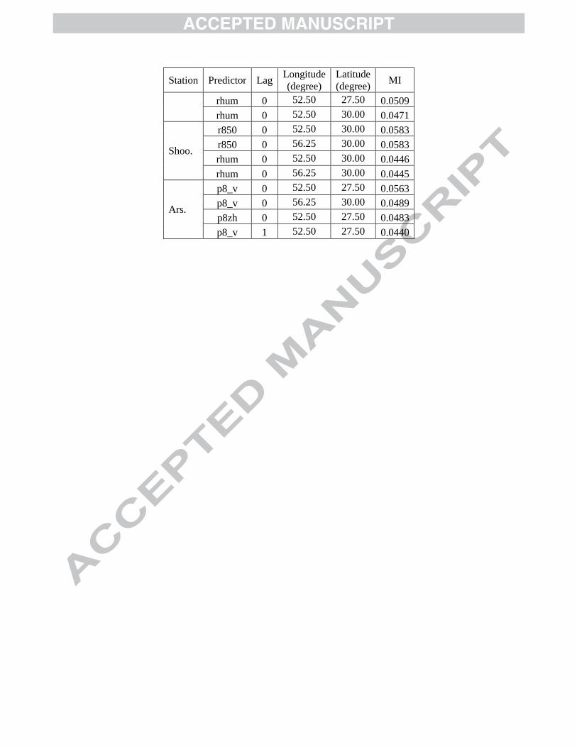
To implement NDMDM, in the first step, suitable predictors must been extracted from the 340
pool of meteorological predictors. Based on the presented description in the section 3.6, MI 341
index has been calculated for different combinations of predictors and predictands to select 342
the suitable predictors. The first five predictors with highest MI values for each predictand 343
are selected. The MI range of the selected predictors is between 0.011 to 0.09. The selected 344
predictors are mostly relative humidity and zonal velocity in different geopotential heights 345
without any time lag. The selected predictors are scattered in all of the nine neighboring 346
boxes shown in Fig. 1. Tables 3 and 4 show the selected five and four predictors set for 347
occurrence and amount models for all of the stations. In these tables, MI values between the 348
predictands and selected predictors have been presented as well. Based on these tables, for 349
occurrence and amount simulation five and four predictors with one lags have been selected 350
(Far. and Khan. stations for occurrence and Ars., Khan. and Deh. Stations for amount) 351
respectively. Relative humidity has been detected as the most selected predictor for both 352
occurrence and amount models all of the stations. Using NDMDM, a set of occurrence and 353
amount models have been calibrated automatically for each month and then stochastic 354
weather generation has been performed for all twenty five possible combinations of five 355
models for occurrence and five models for amount estimation. 356
Number of generated ensembles in each downscaling simulation is set to 100 and also all 357
of the selected models have passed the singularity test as explained in the previous section. In 358
the case of GA-SVM, the population size and cross-over and mutation rates of GA have been 359

16
set to 50, 10% and 80%, respectively; the selected SVM type is epsilon-SVM for both 360
precipitation amount and occurrence models. 361
Sample results obtained from NDMDM for various combinations of the amount and 362
occurrence models for Del. Station are presented in Table 5. To achieve a good perspective of 363
seasonal performance of NDMDM, these results have been categorized to wet (November to 364
April) and dry (May to October) seasonal. In Del. Station, MT-MLR has been found as the 365
best combination of occurrence-amount models. In Table 6, the best combinations of 366
NDMDM models (both occurrence and amount models) for the twelve stations are presented 367
as well. 368
According to the Table 6, MT, MARS, MLR and kNN have been selected 17, 4, 2 and 1 369
times, respectively. Selected DM methods in occurrence mode are only MT and MARS. The 370
most important similarity of these two models is data-partitioning in developing its regression 371
based model structures and this might be the most important reason of their better 372
performance in precipitation occurrence modeling versus the other nonlinear methods used in 373
this study. 374
Table 7 depicts the comparison between statistical characteristics of MLRDM 375
(downscaling using MLR method for both occurrence and amount modeling which is similar 376
to SDSM), selected NDMDM models (based on the proposed FER criteria) and observations 377
in the rain gauge stations in dry and wet seasons and also for the calibration and validation 378
periods. Based on the illustrated results in Table 7, the mean values of the down scaled 379
precipitation series estimated by NDMDM in 58 and 42 percent of the selected rain gauge 380
stations in the calibration and validation periods, respectively have been closer to the 381
historical mean values than the MLRDM model results. In other words, overall NDMDM and 382
MLRDM performances in regenerating mean values are competitive however MLRDM 383
performance is slightly better than NDMDM. 384

17
Table 7 also shows that the standard deviation and skewness values of the down scaled 385
precipitation series estimated by NDMDM in 89 and 92 percent of the selected rain gauge 386
stations in the calibration and validation periods, respectively have been closer to the 387
historical values than the MLRDM model results. In other words, NDMDM shows significant 388
superiority over MLRDM in preserving historical standard deviation and skewness values of 389
the precipitation series. Comparison between the performances of NDMDM in dry and wet 390
seasons also shows that NDMDM performs better in preserving historical mean precipitation 391
of the dry season. 392
The results of the three selected stations (Del., Kas. and Khan.) including monthly mean, 393
monthly standard deviation, monthly skewness and q-q plot of observed versus computed 394
values are shown in Figs. 3, 4 and 5 for the calibration and validation periods. Both MRLDM 395
(MLR-MLR combination which is similar to MLRDM) and NDMDM performances have 396
been acceptable in simulating the monthly mean precipitation values for the calibration and 397
validation periods. For nearly all of the presented q-q plots, a threshold can be found; 398
simulated daily precipitation values larger than this threshold are less than observations. For 399
Del. Station this threshold is about 4.5 mm. For the Ras. Station, this threshold is 8 mm with 400
the exception of NDMDM in the validation period. It is 4 mm for Khan. Station with the 401
exception of the validation period. 402
In Table 8, number of available samples used for occurrence and amount modeling in the 403
calibration period for Del. Station is presented. Number of the parameters for different 404
NDMDM models is also shown in this Table. Number of parameters in MARS and MT are 405
automatically set according to the available samples avoiding over-fitting. In occurrence 406
simulation of the calibration period, many samples are available and models with higher 407
numbers of parameters than MLR are also acceptable. But in simulation of amount in the dry 408
season which has fewer samples, MARS and MT automatically determine suitable number of 409

18
parameters as shown in the Table. For example, in June and September which are the months 410
with fewest samples for amount modeling, both calibrated MT and MARS model have only 411
one parameter while MLR has 5 parameters. GA-SVM also has 6 parameters which can 412
cause over fitting in the dry season for Stations with few precipitation observations. 413
To evaluate the climate change impacts on the studied Stations, SRES A2 and B2 414
scenarios have been considered for the years 2000 to 2050. The results of downscaling using 415
MLRDM and NDMDM are generally different because of the different values of bias 416
correction and variance inflation factors calculated in the calibration period by these models. 417
In Fig. 6, 5-year moving average of precipitation is presented for A2 and B2 scenarios in 418
Del., Ras. and Khan. Stations. As it can be seen in Fig 6, except for Khan. Station, the 419
NDMDM has produced significantly different results compared with MLRDM model. For 420
example, the results of downscaling simulation for Del. Station with MLRDM are 421
significantly higher than the result of NDMDM and for Ras. Station, it is vise-versa. 422
Also in Table 9, some statistical properties of the estimated annual precipitation by 423
MLRDM and NDMDM for the all stations are reported. Based on the table, except for Kas, 424
and Far. Stations, NDMDM and MLRDM results have been relatively similar for each of the 425
scenarios. In other words, if long-term maximum values in one scenario by one model have 426
been increased or decreases, same type of variation have been also predicted by the other 427
model. This similarity of behavior have been also observed for minimum values in all 428
stations except for Shan., Deh., and Shoo. Stations. It also worth mentioning that in both 429
scenarios in almost 75% of the stations, lower minimum values have been estimated by 430
NDMDM compared with MLRDM. Higher variances have also been estimated by NDMDM 431
for all of the stations except for Khan., Shap., and Del. Stations. 432
These results demonstrate high uncertainty associated with downscaling model structures 433
in the climate change modeling for different climate regions and future scenarios. 434

19
435
5. Conclusions 436
The results of this study have shown that different combinations of DM methods can 437
provide good alternative approaches in empirical or regression based downscaling 438
simulations. NDMDM is also proved to be useful software for statistical downscaling. The 439
proposed approach is applicable for downscaling of all meteorological variables and there is 440
no restriction for using NDMDM for other variables however some tuning might be 441
necessary for example for singularity test threshold. 442
Based on the illustrated results of MARS and MT models, it can be concluded that data 443
partitioning plays an important role in similarity of the statistical downscaling results. So, 444
detection of similarity is highly recommended as one of the most important pre-processing 445
steps in statistical downscaling. 446
This study also shows that appropriate performance of NDMDM results is not only 447
related to the complexity of the selected DM methods and their higher numbers of 448
parameters. For example GA-SVM provides much better results in amount simulation 449
compared with MLR while they have almost same number of parameters. As another 450
evidence, kNN (with only one parameter, k) is the selected model for downscaling of Sha. Station 451
while MLR (with 5 parameters) is selected only twice. The results of this study show that the 452
statistical downscaling model performance is highly related to the modeling concept and the 453
overall performance of the occurrence-amount simulation. 454
Occurrence simulation is very similar to pattern recognition and regression based SVM 455
does not provide good results in pattern detection. It is expected that SVM for classification 456
provides better results in occurrence modeling but because of using SDSM platform, it has 457
not been a choice in this study. Presented results in this paper depict better performance of 458
NDMDM in preserving historical monthly mean of precipitation in dry seasons compared 459

20
with wet seasons and closer estimation of historical monthly standard deviation and skewness 460
values compared with MLRDM. Overall the results of this study have shown that NDMDM 461
can be a useful tool for statistical downscaling of precipitation in semi-arid regions with high 462
seasonal variability of precipitation and long dry seasons. 463
Significant uncertainties in projection of climate change effects on precipitation in this 464
study shows that future works can be focused on uncertainty assessment of MLRDM and 465
NDMDM models. These simulations also help in evaluating the mathematical stability of 466
regression models and their parameters. Comparison of the presented approaches in 467
downscaling of other climatic parameters such as temperature, evaporation and number of 468
days with event in Stations is also recommended. 469
470

21
6. References 471
Aizerman, M., Braverman, E., Rozonoer, L., 1964. Theoretical foundations of the potential 472
function method in pattern recognition learning. Automation and Remote Control 25, 473
821-837, 474
Anandhi, A., Frei, A., Pierson, D.C., Schneiderman, E.M., Zion, M.S., Lounsbury, D., 475
Matonse, A.H., 2011. Examination of change factor methodologies for climate change 476
impact assessment. Water Resour Res, 47, W03501, doi: 10.1029/2010WR009104 477
Bárdossy, A., Plate, E.J., 1992. Space-time model for daily rainfall using atmospheric 478
circulation patterns. Water Resour Res, 28(5), 1247–1259 479
Bárdossy, A., Stehlík, J., Caspary, H-J., 2002. Automated objective classification of daily 480
circulation patterns for precipitation and temperature downscaling based on optimized 481
fuzzy rules. Clim Res, 23, 11–22 482
Bates, B. C., Charles, S.P., Hughes, J.P., 1998. Stochastic downscaling of numerical climate 483
model simulations. Environ Modell Softw., 13, 325–331 484
Battiti, R., 1994. Using mutual information for selecting features in supervised neural net 485
learning. IEEE Transactions on Neural Networks, 5 (4), 537–550. 486
Becker, A., 1976, Simulations of nonlinear flow systems by combining linear models. IAHS 487
116, 135-142 488
Becker, A., Kundzewicz, Z.W., 1987. Nonlinear flood routing with multi linear models. 489
Water Resour Res, 23 (6), 1043-1048 490
Bowden, G. J., Dandy, G. C., Maier, H. R., 2005 a. Input determination for neural network 491
models in water resources applications Part 1—background and methodology. Journal of 492
Hydrology, 301(1-4), 75-92 493
22
Bowden, G. J., Maier, H. R., Dandy, G. C., 2005 b. Input determination for neural network 494
models in water resources applications Part 2. Case study: forecasting salinity in a river. 495
Journal of Hydrology, 301(1-4), 93-107 496
Boser, B. E., Guyon, I. M., Vapnik, V. N., 1992. A training algorithm for optimal margin 497
classifiers. In D. Haussler, editor, 5th Annual ACM Workshop on COLT, Pittsburgh, 498
PA, ACM Press,144-152, 499
Buccola, N.L., Wood, T.M., 2010. Empirical models of wind conditions on Upper Klamath 500
Lake. Oregon. U.S. Geological Survey Scientific-Investigations Report 2010–5201 501
Chen, S.T., Yu, P.S., Tang, Y.H., 2010. Statistical Downscaling of Daily Precipitation using 502
Support Vector Machines and Multivariate Analysis. J Hydrol, 385(1-4), 13-22 503
Coulibaly, P., Baldwine, C. K., 2005. Non stationary hydrological time series forecasting 504
using nonlinear dynamic methods. J Hydrol, 307, 164-174 505
Cover, T. M., 1965. Geometrical and Statistical Properties of Systems of Linear Inequalities 506
with Applications in Pattern Recognition. IEEE Trans. Elec. Comp., EC-14, 326-334. 507
Corte-Real, J., Zhang, X. and Wang, X. 1995. Downscaling GCM information to regional 508
scales: a non-parametric multivariate regression approach. Climate Dynamics, 11, 413–509
424. 510
Enke, W., Spekat, A., 1997. Downscaling climate model outputs into local and regional 511
weather elements by classification and regression. Clim Res, 8, 195-207 512
Faucher, M., Burrows, W.R., Pandolfo, L., 1999. Empirical-statistical reconstruction of 513
surface marine winds along the western coast of Canada. Clim Res, 11, 173-190 514
Fei, Sh. W., Sun, Y., 2008. Forecasting dissolved gases content in power transformer oil 515
based on support vector machine with genetic algorithm. Electric Power Systems 516
Research, 78 (3), 507-514 517

23
Fistikoglu, O., Okkan. U., 2011. Statistical Downscaling of Monthly Precipitation Using 518
NCEP/NCAR Reanalysis Data for Tahtali River Basin in Turkey. J Hydrol. Eng., 16(2), 519
doi:10.1061/(ASCE)HE.1943-5584.0000300 520
Friedman, J.H., Stuetzle, W., 1981. Projection pursuit regression. JASA, 76, 817–823 521
Friedman, J.H., 1991. Multivariate Adaptive Regression Splines. Ann Stat, 19(1), 1–67 522
Friedman, J.H., 1993. Fast MARS. Dept. of Statistics, Stanford University, Technical Report: 523
110, 524
Gangopadhyay, S., Clark, M., Rajagopalan, B., 2005, Statistical Downscaling using K-525
nearest neighbors. Water Resour Res, 41, W02024, doi:10.1029/2004WR003444 526
Guyon, I., Elisseeff, A., 2003. An introduction to variable and feature Selection. Journal of 527
Machine Learning Research, 3, 1157-1182. 528
Herrera, M., Torgo, L., Izquierdo, J., Perez-Garcia, R., 2010. Predictive models for 529
forecasting hourly urban water demand. J Hydrol, 384, 141-150 530
Hessami, M., Gachon, Ph., Ouarda, T.B.M.J., St-Hilaire, A., 2008. Automated regression-531
based statistical downscaling tool. Environ Modell Softw. 23(6), 813-834 532
Hoerl, A.E., Kennard, R.W., 1970. Ridge regression: application to nonorthogonal problems. 533
Technometrics 12 (1), 69-82 534
Jekabsons, G., 2010, ARESLab: Adaptive Regression Splines toolbox for Matlab/Octave. 535
available at http://www.cs.rtu.lv/jekabsons/ 536
Jekabsons, G., 2010. M5PrimeLab: M5' regression tree and model tree toolbox for Matlab. 537
available at http://www.cs.rtu.lv/jekabsons/ 538
Li, X., Sailor, D., 2000. Application of tree-structured regression for regional precipitation 539
prediction using general circulation model output. Clim Res, 16, 17-30 540
Liue, H., Yu, L., 2005. Toward integrating feature selection algorithms for classification and 541
clustering. IEEE Transactions on Knowledge and Data Engineering, 17(4), 491-502. 542

24
Lall, U., Sharma, A., 1996. A nearest neighbor bootstrap for resampling hydrologic time 543
series. Water Resources Research, 32(3), 679-693 544
May, R. J., Dandy, G. C., Maier, H. R., Nixon, J. B., 2008a. Application of partial mutual 545
information variable selection to ANN forecasting of water quality in water distribution 546
systems. Environmental Modeling and Software, 23, 1289-1299 547
May, R. J., Maier, H. R., Dandy, G. C., Fernando, T. G., 2008b. Non-linear variable selection 548
for artificial neural networks using partial mutual information. Environmental Modeling 549
and Software, 23, 1312-1326. 550
Mendes, D., Marengo, J.A., 2010. Temporal downscaling: a comparison between artificial 551
neural network and autocorrelation techniques over the Amazon Basin in present and 552
future climate change scenarios. Theor Appl Climatol, 100 (3-4), 413-421 553
Oliveira, A. L. I., Braga, P.L., Lima, R. M. F., Cornélio, M. L., 2010. GA-based method for 554
feature selection and parameters optimization for machine learning regression applied to 555
software effort estimation, Information and Software Technology, 52(11), 1155-1166 556
Pasini, A., 2009. Neural Network Modelling in Climate Change Studies. Artificial 557
Intelligence Methods in the Environmental Sciences II, 413-421 558
Quinlan, J. R., 1986. Induction on decision trees. Mach Learn 1, 81-106. 559
Quinlan, J. R., 1993. C4.5: Programs for Machine Learning. San Mateo, CA: Morgan 560
Kaufmann 561
Raje, D., Mujumdar, P.P., 2011. A comparison of three methods for downscaling daily 562
precipitation in the Punjab region. Hydrol Process, doi:10.1002/hyp.8083 563
Semenov, M.A., Barrow, E., 1997. Use of stochastic weather generator in the development of 564
climate change scenarios. Clim. Change, 35, 397–414 565
Sharif, M., Burn, D. H., 2006. Simulating climate change scenarios using an improved K-566
nearest neighbor model. Journal of Hydrology, 325, 179-196 567

25
Solomatine, D., Dulal, K. h., 2003. Model trees as an alternative to neural networks in 568
rainfall-runoff modeling. Hydrolog. Sci. J., 48, 399-411 569
Solomatine, D., Xue, Y., 2004, M5 model trees and neural networks: application to flood 570
forecasting in the upper reach of the Huai river in China. J. Hydrol. Eng., 9(6), 275-287 571
Tan, P. N., Steinbach, M., Kumar, V., 2006. Introduction to data mining. Addison Wesley, 572
Tomassetti, B., Verdecchia, M., Giorgi, F., 2009. NN5: A neural network based approach for 573
the downscaling of precipitation fields–Model description and preliminary results. J 574
Hydrol, 367(1-2), 14-26 575
Tripathi, Sh., Srinivas, V. V., Nanjundiah, R. S., 2006. Downscaling of Precipitation for 576
Climate Change Scenarios: A Support Vector Machine Approach. J Hydrol 330(3-4), 577
621-640 578
Xiong, L. H., Shamseldin, A. Y., O’Connor, K. M., 2001. A non-linear combination of the 579
forecasts of rainfall–runoff models by the first-order Takagi-Sugeno. fuzzy system. J 580
Hydrol. 245(1–4), 196–217, 581
Vapnik, V. N., Cortes, C., 1995. Support vector networks. Machine Learning, 20, 273–297. 582
Vapnik, V. N., 1998. Statistical Learning Theory. Wiley, New York. 583
Wang. Y., Witten, I. H., 1997. Induction of model trees for predicting continuous classes. 584
Proceedings of European Conference on Machine Learning, Prague, 128-137 585
Wetterhall, F., Bárdossy, A., Chen, D., Halldin, S., Xu, Ch., 2009, Statistical downscaling of 586
daily precipitation over Sweden using GCM output. Theor Appl Climatol, 96, 95–103 587
Wilby, R. L., Hay, L. E., Leavesley, G. H., 1999. A comparison of downscaled and raw GCM 588
output: implications for climate change scenarios in the San Juan River basin, Colorado. 589
J Hydrol, 225, 67–91 590
Wilby, R. L., Dawson, C. W., Barrow, E. M., 2002. SDSM–a decision support tool for the 591
assessment of regional climate change impacts. Environ Modell Softw, 17, 147–159 592
26
Wilby, R. L., Charles, S. P., Zorita, E., Timbal, B., Whetton, P., Mearns, L. O., 2004. 593
Guidelines for use of climate scenarios developed from statistical downscaling methods. 594
Supporting material of the Intergovernmental Panel on Climate Change, available from 595
the DDC of IPCC TGCIA, 27 596
Yarnal, B., Comrie, A. C., Frakes, B., Brown, D. P., 2001. Developments and prospects in 597
synoptic climatology. Int J Climatol, 21, 1923–1950 598
Yates, D., Gangopadhyay, S., Rajagopalan, B., Strzepek, K., 2003. A Technique for 599
Generation Regional Climate Scenarios using a Nearest-Neighbor Algorithm. Water 600
Resour Res, 39(7), 1199, doi:10.1029/2002WR001769 601

Table 1.Basic information about 12 rain gauge stations (Max.=Maximum and Std.=Standard deviation)
No. Station code Station name Abbr. Basin
Length of
Dataset
(year)
Longitude
(°E)
Latitude
(°N)
Statistical characteristics of
observed daily rainfall (mm)
Mean Max. Std. 1 44-014 Delfard Del. Jazmoorian
1975–2000
57.60 29.00 1.20 150 6.31
2 44-009 Dehrood Deh. Jazmoorian 57.73 28.87 0.76 132 4.71
3 44-016 Khoramshahi Kho. Jazmoorian 57.75 29.00 1.32 194 6.95
4 44-024 Kharposht Khar. Jazmoorian 57.83 28.48 0.46 80 3.20
5 17-082 Rasht Ras. Sefidrood
1966–2000
49.60 37.25 3.58 188 10.34
6 17-075 Farshekan Far. Sefidrood 49.58 37.40 3.30 168 9.93
7 18-007 Kasma Kas. Mordab-anzali 49.30 37.31 3.01 317 9.59
8 18-017 Shanderman Shan. Mordab-anzali 49.11 37.41 2.67 177 8.23
9 24-033 Khanzanian Khan. Mond
1972–2000
52.15 29.67 1.27 92 5.26
10 23-011 Shapoor Shap. Shapoor-dalky 51.11 29.58 0.85 75 4.45
11 23-019 Shoorjareh Shoo. Shapoor-dalky 51.98 29.25 0.99 120 4.92
12 43-034 Arsanjan Ars. Shapoor-dalky 51.30 29.92 0.87 111 4.56

Table 2. Large-scale Predictors from NCEP database
No. Predictor Abbreviation
1 Mean Sea Level Pressure mslp
2 Surface Airflow Strength p__f
3 Surface Zonal Velocity p__u
4 Surface Meridional Velocity p__v
5 Surface Vorticity p__z
6 Surface Wind Direction p_th
7 Surface Divergence p_zh
8 500 hpa Airflow Strength p5_f
9 500 hpa Zonal Velocity p5_u
10 500 hpa Meridional Velocity p5_v
11 500 hpa Vorticity p5_z
12 500 hpa Wind Direction p5th
13 500 hpa Divergence p5zh
14 850 hpa Airflow Strength p8_f
15 850 hpa Zonal Velocity p8_u
16 850 hpa Meridional Velocity p8_v
17 850 hpa Vorticity p8_z
18 850 hpa Wind Direction p8th
19 850 hpa Divergence p8zh
20 500 hpa Geopotential Height p500
21 850 hpa Geopotential Height p850
22 Relative Humidity at 500 hpa r500
23 Relative Humidity at 850 hpa r850
24 Near Surface Relative Humidity Rhum
25 Near Surface Specific Humidity Shum
26 Mean Temperature at 2m Temp

Table 3. Selected predictors for occurrence model calibrated for different stations
Station Predictor Lag Longitude
(degree)
Latitude
(degree) MI
Del.
rhum 0 56.25 30.00 0.0170
r850 0 56.25 30.00 0.0170
r850 0 60.00 27.50 0.0165
r850 0 56.25 27.50 0.0162
p500 0 52.50 30.00 0.0162
Deh.
r850 0 56.25 27.50 0.0169
r850 0 56.25 30.00 0.0161
r850 0 60.00 27.50 0.0161
rhum 0 56.25 27.50 0.0152
rhum 0 56.25 30.00 0.0152
Kho.
p500 0 52.50 30.00 0.0209
pr850 0 52.50 32.50 0.0207
pr850 0 56.25 27.50 0.0197
pr850 0 60.00 27.50 0.0190
rhum 0 56.25 27.50 0.0181
Khar.
r850 0 56.25 27.50 0.0113
r850 0 56.25 30.00 0.0113
r850 0 60.00 27.50 0.0112
rhum 0 56.25 27.50 0.0111
rhum 0 56.25 30.00 0.0110
Ras.
r850 0 48.75 37.50 0.0493
r850 0 48.75 40.00 0.0429
rhum 0 48.75 37.50 0.0380
r850 0 52.50 37.50 0.0328
p__u 0 48.75 40.00 0.0299
Far.
r850 0 48.75 37.50 0.0490
r850 0 48.75 40.00 0.0456
r850 0 52.50 37.50 0.0379
rhum 0 48.75 37.50 0.0335
r850 1 48.75 40.00 0.0319
Kas.
p__u 0 48.75 40.00 0.0449
r850 0 48.75 37.50 0.0426
r850 0 48.75 40.00 0.0352
r850 0 52.50 37.50 0.0320
rhum 0 48.75 37.50 0.0283
Shan.
p__u 0 48.75 40.00 0.0407
p__z 0 48.75 40.00 0.0394
pr850 0 48.75 37.50 0.0308

Station Predictor Lag Longitude
(degree)
Latitude
(degree) MI
pr850 0 48.75 40.00 0.0304
rhum 0 48.75 37.50 0.0258
Khan.
rhum 0 52.50 30.00 0.0436
r850 0 52.50 30.00 0.0436
r850 0 48.75 30.00 0.0366
r850 0 52.50 27.50 0.0350
p8zh 1 48.75 27.50 0.0350
Shap.
r850 0 48.75 30.00 0.0473
r850 0 48.75 32.50 0.0472
r850 0 52.50 27.50 0.0394
r850 0 52.50 30.00 0.0387
rhum 0 52.50 30.00 0.0358
Shoo.
r850 0 48.75 30.00 0.0485
r850 0 52.50 27.50 0.0485
r850 0 52.50 30.00 0.0412
rhum 0 52.50 30.00 0.0384
rhum 0 56.25 30.00 0.0382
Ars.
r850 0 52.50 27.50 0.0459
r850 0 52.50 30.00 0.0459
r850 0 56.25 30.00 0.0389
rhum 0 52.50 30.00 0.0389
rhum 0 56.25 30.00 0.0359

Table 4. Selected predictors for the amount model calibrated for different stations
Station Predictor Lag Longitude
(degree)
Latitude
(degree) MI
Del.
p5zh 0 52.50 30.00 0.0515
p5zh 0 56.25 27.50 0.0511
p5_v 0 56.25 30.00 0.0508
p5_v 0 52.50 30.00 0.0489
Deh.
r850 0 56.25 52.50 0.0538
rhum 0 56.25 27.50 0.0521
r850 1 56.25 30.00 0.0520
rhum 1 56.25 30.00 0.0492
Kho.
p5_v 0 52.50 27.50 0.0482
p5_v 0 52.50 30.00 0.0475
p5_v 0 52.50 32.50 0.0471
p5zh 0 52.50 27.50 0.0452
Khar.
r850 0 60.00 27.50 0.0879
r850 0 60.00 30.00 0.0849
rhum 0 56.25 27.50 0.0808
rhum 0 60.00 30.00 0.0771
Ras.
p8th 0 52.50 40.00 0.0243
p__u 0 48.75 37.50 0.0225
p8th 0 52.50 37.50 0.0223
p__u 0 45.00 40.00 0.0215
Far.
p__u 0 45.00 40.00 0.0242
p__u 0 48.75 37.50 0.0217
p8th 0 52.50 40.00 0.0217
r850 0 48.75 37.50 0.0215
Kas.
p__u 0 45.00 37.50 0.0140
p__u 0 48.75 37.50 0.0137
p8_u 0 45.00 37.50 0.0136
p8th 0 45.00 37.50 0.0135
Shan.
p__u 0 45.00 40.00 0.0194
p__z 0 48.75 40.00 0.0175
p8_u 0 45.00 37.50 0.0168
p8th 0 52.50 40.00 0.0166
Khan.
r850 0 52.50 30.00 0.0522
rhum 0 52.50 30.00 0.0522
p8_v 1 52.50 27.50 0.0434
p8_v 0 56.25 30.00 0.0431
Shap. p8_v 0 56.25 32.50 0.0624
r850 0 52.50 30.00 0.0618
Station Predictor Lag Longitude
(degree)
Latitude
(degree) MI
rhum 0 52.50 27.50 0.0509
rhum 0 52.50 30.00 0.0471
Shoo.
r850 0 52.50 30.00 0.0583
r850 0 56.25 30.00 0.0583
rhum 0 52.50 30.00 0.0446
rhum 0 56.25 30.00 0.0445
Ars.
p8_v 0 52.50 27.50 0.0563
p8_v 0 56.25 30.00 0.0489
p8zh 0 52.50 27.50 0.0483
p8_v 1 52.50 27.50 0.0440

Table 5. NDMDM results for Del. Station (based on the validation period)
Model Combination Dry Season Wet Season
FER N
o
Occurren
ce Model
Amount
Model Mean
Standard
Deviation. Skewness Mean
Standard
Deviation. Skewness
1 MLR MLR 0.27 0.51 3.92 1.98 2.96 2.59 0.4
2 MLR kNN 0.25 0.44 4.23 1.93 2.83 3.23 0.4
3 MLR MARS 0.25 0.41 3.73 1.97 2.83 3.46 0.41
4 MLR MT 0.27 0.44 3.06 1.94 2.88 3.15 0.43
5 MLR GA-
SVM 0.28 0.53 8.22 2.16 2.76 2.1 0.37
6 kNN MLR 0.16 0.54 4.33 1.84 3.56 3 0.35
7 kNN kNN 0.14 0.47 5.1 1.78 3.23 2.94 0.4
8 kNN MARS 0.15 0.58 11.64 1.87 3.68 5.51 0.27
9 kNN MT 0.16 0.49 4.22 1.78 3.51 4.82 0.35
10 kNN GA-
SVM 0.17 0.64 10.34 1.93 3.23 2.17 0.29
11 MARS MLR 0.75 1.81 2.96 1.93 3.56 3.41 0.6
12 MARS kNN 0.67 1.62 3.15 1.88 3.34 3.79 0.48
13 MARS MARS 0.77 1.87 2.86 1.97 3.92 9.19 0.61
14 MARS MT 0.8 1.94 3.06 1.89 3.49 4.74 0.66
15 MARS GA-
SVM 0.82 1.97 2.96 2.08 3.21 2.39 0.71
16 MT MLR 0.17 1.16 12.27 2.07 5.02 2.82 0.07
17 MT kNN 0.14 0.99 13.89 2.05 4.9 2.95 0.15
18 MT MARS 0.15 1.11 17.73 2.11 4.98 3.59 0.13
19 MT MT 0.17 1.03 8.97 2.07 4.93 2.99 0.09
20 MT GA-
SVM 0.22 2.15 25.04 2.22 4.87 2.25 0.26
21 GA-
SVM MLR 0.29 0.7 9.56 1.75 1.46 1.07 0.42
22 GA-
SVM kNN 0.24 0.54 8.41 1.82 1.47 1.34 0.43
23 GA-
SVM MARS 0.25 0.53 10.29 1.85 1.38 1.34 0.43
24 GA-
SVM MT 0.27 0.51 5.73 1.81 1.6 3.79 0.45
25 GA-
SVM
GA-
SVM 0.29 0.64 12.28 2.13 1.58 1.78 0.42
Observation 0.2 1.48 9.93 2.33 8.72 6.23 -
*Selected combination of the amount and occurrence models are marked in gray color.

Table 6. Best combination of occurrence and amount models in the twelve rain gauge stations
No. Station Occurrence
Model
Amount
model
1 Del. MT MLR
2 Deh. MT MARS
3 Kho. MT MT
4 Khar. MARS MT
5 Ras. MARS MT
6 Far. MT MT
7 Kas. MARS MT
8 Shan. MT MT
9 Khan. MT MT
10 Shap. MT kNN
11 Shoo. MT MLR
12 Ars. MT MT

Table 7. Comparison of statics of daily precipitation values downscaled by MLRDM and
NDMDM
Station Model
Calibration Validation
Dry Season Wet Season Dry Season Wet Season
Mean Std. Skw. Mean Std. Skw. Mean Std. Skw. Mean Std. Skw.
Del.
MLRDM 0.35 0.89 5.35 2.18 4.22 4.68 0.35 0.84 3.82 2.26 4.17 3.28
NDMDM 0.2 0.99 6.58 2.04 5.36 3.61 0.17 1.16 12.27 2.07 5.02 2.82
Obs. 0.28 2.58 22.40 2.12 8.47 8.20 0.20 1.48 9.93 2.33 8.72 6.23
Deh.
MLRDM 0.15 0.54 9.03 1.49 2.99 4.16 0.18 0.54 5.74 1.50 2.86 2.94
NDMDM 0.12 0.73 9.54 1.48 4.58 4.95 0.11 0.64 7.77 1.59 4.63 4.3
Obs. 0.12 1.59 19.96 1.47 6.78 7.76 0.08 0.95 20.12 1.29 5.32 5.94
Kho.
MLRDM 0.26 0.77 10.91 2.61 4.89 3.38 0.21 0.63 6.55 2.72 4.84 2.81
NDMDM 0.22 1.17 7.37 2.45 7.21 5.9 0.16 0.97 7.65 2.29 6.12 4.05
Obs. 0.23 1.99 14.27 2.55 9.63 6.77 0.20 1.52 10.84 2.08 9.28 8.45
Khar.
MLRDM 0.11 0.37 8.17 0.90 1.85 3.66 0.13 0.39 4.42 0.97 1.90 3.18
NDMDM 0.09 0.41 18.76 0.89 2.57 6.12 0.12 0.63 14.62 0.9 2.61 6.95
Obs. 0.07 1.02 24.68 0.87 4.55 7.95 0.12 1.53 22.28 0.76 3.63 6.39
Ras.
MLRDM 2.89 5.51 4.08 4.05 5.95 2.35 3.01 6.36 3.91 4.30 6.60 2.57
NDMDM 3.01 6.96 5.21 4.01 6.97 4.04 3.04 7.87 5.04 4.16 7.76 3.89
Obs. 3.00 10.28 6.62 4.16 10.33 4.71 3.44 11.31 6.06 3.77 9.38 4.12
Far.
MLRDM 2.66 5.36 4.01 3.70 5.36 2.29 2.64 5.93 3.72 3.91 5.93 2.51
NDMDM 2.63 7.41 4.68 3.67 7.34 3.32 1.68 6.17 6.11 3.74 7.85 3.53
Obs. 2.69 9.52 6.29 3.79 9.64 4.92 3.16 11.47 6.77 3.78 10.20 4.54
Kas.
MLRDM 3.04 5.02 3.31 2.93 4.17 2.48 2.79 5.55 3.68 2.74 4.32 2.88
NDMDM 3.14 7.06 5.72 3.03 5.44 4.2 2.88 7.72 5.81 2.89 5.59 4.12
Obs. 3.02 11.47 9.49 3.06 7.84 4.57 3.07 10.24 5.84 2.76 7.15 4.46
Shan.
MLRDM 2.81 4.13 2.86 2.48 2.90 1.83 2.63 4.63 3.10 2.37 3.18 2.86
NDMDM 2.8 6.82 4.72 2.55 5.2 5.76 2.12 6.52 5.93 2.47 5.6 6.78
Obs. 2.81 9.72 7.00 2.54 6.59 6.97 2.87 9.45 6.35 2.40 6.08 4.50
Khan.
MLRDM 0.20 0.72 7.13 2.33 4.12 2.82 0.21 0.70 6.11 2.36 4.47 3.16
NDMDM 0.14 1.08 12.85 2.3 5.21 3.39 0.08 0.57 11.86 2.35 5.64 3.69
Obs. 0.15 1.61 16.93 2.39 7.08 4.58 0.12 1.20 17.40 2.48 7.29 3.81
Shap.
MLRDM 0.07 0.53 22.94 1.51 3.40 3.58 0.06 0.37 12.27 1.58 3.52 3.55
NDMDM 0.06 0.7 20.78 1.5 4.01 3.69 0.03 0.5 23.65 1.33 3.81 3.95
Obs. 0.07 1.20 24.90 1.57 5.87 5.70 0.03 0.49 18.24 1.90 6.77 5.31
Shoo.
MLRDM 0.07 0.30 10.73 1.80 3.68 3.21 0.07 0.24 5.41 1.75 3.60 3.29
NDMDM 0.07 0.64 15.6 1.86 4.43 2.92 0.06 0.63 18.41 1.82 4.46 2.95
Obs. 0.07 0.91 19.45 1.83 6.53 6.59 0.06 0.74 19.86 2.24 7.53 5.01
Ars.
MLRDM 0.24 0.90 7.25 1.59 3.85 4.85 0.37 1.38 6.77 1.82 4.15 3.83
NDMDM 0.08 0.55 11.91 1.56 4.7 6.55 0.07 0.49 11.03 1.69 5.11 5.85
Obs. 0.09 1.19 23.65 1.62 6.10 6.99 0.05 0.71 23.11 1.79 6.78 5.89

Table 8. Number of Parameters for amount and occurrence models and number of the available
samples in Del. Station in the calibration period,
Model DM Method Jan Feb Mar Apr May Jun Jul Aug Sep Oct Nov Dec
Occ
urr
ence
Sim
ula
tion
MLR 6 6 6 6 6 6 6 6 6 6 6 6
kNN 1 1 1 1 1 1 1 1 1 1 1 1
MARS 29 16 31 29 31 34 29 21 31 31 34 29
MT 48 50 54 29 17 9 16 22 7 17 11 40
GA-SVM 6 6 6 6 6 6 6 6 6 6 6 6
No. of Samples 620 565 612 570 589 570 589 589 578 620 600 620
Am
ount
sim
ula
tion
MLR 5 5 5 5 5 5 5 5 5 5 5 5
kNN 1 1 1 1 1 1 1 1 1 1 1 1
MARS 6 6 1 1 6 1 1 14 1 1 1 31
MT 9 8 5 2 3 1 3 1 1 1 1 7
GA-SVM 6 6 6 6 6 6 6 6 6 6 6 6
No. of Samples 87 110 121 47 25 7 13 26 7 18 16 69

Table 9. Maximum, Minimum and Variance of annual precipitation of all stations for different
future scenarios
Station Statistics A2 B2
MLRDM NDMDM MLRDM NDMDM
Del.
Maximum 610 497 520 452
Minimum 137 90 188 100
Variance 10692 10554 6090 8259
Deh.
Maximum 610 805 520 797
Minimum 137 156 188 142
Variance 10692 20140 6090 16655
Kho.
Maximum 585 535 582 442
Minimum 159 89 223 111
Variance 7988 10074 4616 4982
Khar.
Maximum 226 311 209 229
Minimum 45 22 66 22
Variance 1730 3380 1168 2226
Ras.
Maximum 1242 2264 1628 2786
Minimum 689 1099 609 1003
Variance 19241 63680 36767 89604
Far.
Maximum 1293 1225 1673 2106
Minimum 693 546 533 464
Variance 23853 30720 41407 91291
Kas.
Maximum 1323 1470 1486 1325
Minimum 792 592 690 492
Variance 18707 31380 25873 33943
Shan.
Maximum 1311 1632 1332 2201
Minimum 707 782 733 600
Variance 13901 46507 17757 84526
Khan.
Maximum 576 533 501 490
Minimum 129 93 132 107
Variance 12005 8839 8659 7614
Shap.
Maximum 462 262 382 261
Minimum 96 45 73 47
Variance 5480 3035 4168 2552
Shoo.
Maximum 93 188 90 193
Minimum 35 28 32 51
Variance 237 1220 197 994
Ars.
Maximum 540 581 416 453
Minimum 83 47 118 70
Variance 10241 12360 6562 7824

Fig. 1. Location map of rain gauge stations in Jazmoorian, Sefidrood, Mordab-anzali, Shapoor-
dalky and Mond basins

Selected
Predictand
Selected
Predictand
Selected
Predictors
Selected
Predictors
· MLR
· kNN
· MARS
· MT
· SVM-GA
· MLR
· kNN
· MARS
· MT
· SVM-GA
Occurrence Model Amount Model
Is the random
number less than the
occurrence model
output?
For each day, in each ensemble and using each model:
Precip.
Doesn’t
occur
Precip.
Doesn’t
occur
Precip.
occurs
Precip.
occursYes
No
Generate a
uniformly
distributed
random number
in [0,1]
Generate a
uniformly
distributed
random number
in [0,1]
Calculate The Amount model’s outputCalculate The Amount model’s output
Add a random number with normal distribution
to the output (Mean=0, Std.=Standard Error)
Add a random number with normal distribution
to the output (Mean=0, Std.=Standard Error)
Compare the result with the thresholdCompare the result with the threshold
Set Model Structure
Select the best combination of
occurrence and amount models
Select the best combination of
occurrence and amount models
· MLR
· kNN
· MARS
· MT
· SVM-GA
· MLR
· kNN
· MARS
· MT
· SVM-GA
Fig.2. NDMDM procedure

Fig.3. Downscaling results for Del. rain gauge
a) Monthly mean, b) Monthly standard deviation, c) Monthly skewness and d) q-q plot of
Monthly precipitation (left column: calibration period, right column: validation period)
0
1
2
3
4
5
1 2 3 4 5 6 7 8 9 10 11 12
Mon
thly
Mea
n (
mm
)
Month
a-2) Observed
MLRDM
NDMDM
0
1
2
3
4
5
1 2 3 4 5 6 7 8 9 10 11 12
Mon
thly
Mea
n (
mm
)
Month
a-1) Observed
MLRDM
NDMDM
0
2
4
6
8
10
12
14
1 2 3 4 5 6 7 8 9 10 11 12
Mon
thly
Std
. (m
m)
Month
b-2) Observed
MLRDM
NDMDM
0
2
4
6
8
10
12
14
1 2 3 4 5 6 7 8 9 10 11 12 M
on
thly
Std
. (m
m)
Month
b-1) Observed
MLRDM
NDMDM
0 2 4 6 8
10 12 14 16 18
1 2 3 4 5 6 7 8 9 10 11 12
Mon
thly
Sk
ewn
ess
(mm
)
Month
c-2) Observed
MLRDM
NDMDM
0
2
4
6
8
10
12
14
16
1 2 3 4 5 6 7 8 9 10 11 12
Mon
thly
Sk
ewn
ess
(mm
)
Month
c-1) Observed
MLRDM
NDMDM
0
1
2
3
4
5
6
0 1 2 3 4 5 6 Mod
eled
Mon
thly
Pre
cip
.
(mm
)
Observed Monthly Precip. (mm)
d-2)
MLRDM
NDMDM
Bisector
0
2
4
6
8
10
0 2 4 6 8 10 Mod
eled
Mon
thly
Pre
cip
.
(mm
)
Observed Monthly Precip. (mm)
d-1)
MLRDM
NDMDM
Bisector

Fig.4. Ras. rain gauge
a) Monthly mean, b) Monthly standard deviation, c) Monthly skewness and d) q-q plot of
monthly precipitation (Left column: calibration period, right column: validation period)
0
1
2
3
4
5
6
7
8
1 2 3 4 5 6 7 8 9 10 11 12
Mon
thly
Mea
n (
mm
)
Month
a-1) Observed
MLRDM
NDMDM
0
2
4
6
8
10
1 2 3 4 5 6 7 8 9 10 11 12
Mon
thly
Mea
n (
mm
)
Month
a-2) Observed
MLRDM
NDMDM
0
5
10
15
20
1 2 3 4 5 6 7 8 9 10 11 12
Mon
thly
Std
. (m
m)
Month
b-1) Observed
MLRDM
NDMDM
0
5
10
15
20
1 2 3 4 5 6 7 8 9 10 11 12
Mon
thly
Std
. (m
m)
Month
b-2) Observed
MLRDM
NDMDM
0
2
4
6
8
10
1 2 3 4 5 6 7 8 9 10 11 12
Mon
thly
Sk
ewn
ess
(mm
)
Month
c-1) Observed
MLRDM
NDMDM
0 1 2 3 4 5 6 7 8 9
1 2 3 4 5 6 7 8 9 10 11 12
Mon
thly
Sk
ewn
ess
(mm
)
Month
c-2) Observed
MLRDM
NDMDM
0
5
10
15
0 5 10 15 Mod
eled
Mon
thly
Pre
cip
.
(mm
)
Observed Monthly Precip. (mm)
d-1)
MLRDM
NDMDM
Bisector
0
2
4
6
8
10
12
14
0 2 4 6 8 10 12 14 Mod
eled
Mon
thly
Pre
cip
.
(mm
)
Observed Monthly Precip. (mm)
d-2)
MLRDM
NDMDM
Bisector
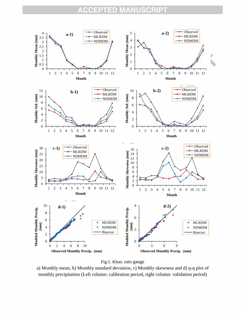
Fig.5. Khan. rain gauge
a) Monthly mean, b) Monthly standard deviation, c) Monthly skewness and d) q-q plot of
monthly precipitation (Left column: calibration period, right column: validation period)
0
0.5
1
1.5
2
2.5
3
3.5
4
1 2 3 4 5 6 7 8 9 10 11 12
Mon
thly
Mea
n (
mm
)
Month
a-1) Observed
MLRDM
NDMDM
0
1
2
3
4
5
1 2 3 4 5 6 7 8 9 10 11 12
Mon
thly
Mea
n (
mm
)
Month
a-2) Observed
MLRDM
NDMDM
0
2
4
6
8
10
12
1 2 3 4 5 6 7 8 9 10 11 12
Mon
thly
Std
. (m
m)
Month
b-1) Observed
MLRDM
NDMDM
0
2
4
6
8
10
1 2 3 4 5 6 7 8 9 10 11 12 M
on
thly
Std
. (m
m)
Month
b-2) Observed
MLRDM
NDMDM
0
5
10
15
20
25
30
1 2 3 4 5 6 7 8 9 10 11 12
Mon
thly
Sk
ewn
ess
(mm
)
Month
c-1) Observed
MLRDM
NDMDM
0
2
4
6
8
10
12
14
16
1 2 3 4 5 6 7 8 9 10 11 12
Mon
thly
Sk
ewn
ess
(mm
)
Month
c-2) Observed
MLRDM
NDMDM
0
2
4
6
8
10
0 2 4 6 8 10 Mod
eled
Mon
thly
Pre
cip
.
(mm
)
Observed Monthly Precip. (mm)
d-1)
MLRDM
NDMDM
Bisector
0
3
6
9
0 3 6 9 Mod
eled
Mon
thly
Pre
cip
.
(mm
)
Observed Monthly Precip. (mm)
d-2)
MLRDM
NDMDM
Bisector

Fig.6. 5-year moving average for A2 and B2 Scenarios in a) Del., b) Ras. and c) Khan. stations
0
100
200
300
400
500
600
20
05
20
10
20
15
20
20
20
25
20
30
20
35
20
40
20
45
20
50
An
nu
al
Pre
cip
(m
m)
a)
MLRDM-A2
MLRDM-B2
NDMDM-A2
NDMDM-B2
700
900
1100
1300
1500
1700
1900
2100
20
05
20
10
20
15
20
20
20
25
20
30
20
35
20
40
20
45
20
50
An
nu
al
Pre
cip
(m
m)
b)
MLRDM-A2
MLRDM-B2
NDMDM-A2
NDMDM-B2
0
100
200
300
400
500
600
20
05
20
10
20
15
20
20
20
25
20
30
20
35
20
40
20
45
20
50
An
nu
al
Pre
cip
(m
m)
c)
MLRDM-A2
MLRDM-B2
NDMDM-A2
NDMDM-B2

Regression-based of downscaling such as SDSM has been coded in MATLAB.
Nonlinear Data-Mining Downscaling Model (NDMDM), as a toolbox, has been programmed.
Four nonlinear and semi nonlinear data-mining method have been implemented in NDMDM.
Twelve rain gauges with different climate have been used as case studies.
Results of NDMDM have been better than statistical downscaling method using three statistical
indices.
*Highlights (for review)