Performance and route stability analysisof RPL protocol

MUHAMMAD RASHID KHAN

Masters’ Degree ProjectStockholm, Sweden May 2012

XR-EE-RT 2012:013

Abstract

Wireless Sensor Networks are getting more deployed in different environ-ment where they provide many benefits for industrial and home automation,smart buildings, medical and environmental monitoring. Sensors are low costdevices with limited storage, computation, and power. Finding optimal basedrouting solutions is a challenging task in wireless sensor networks because ofconstraint over nodes and lossy links. The IETF Routing over Low powerand Lossy network (ROLL) working group has recently developed the IPv6based RPL routing protocol for Low power and Lossy Networks (LLNs). Itis very important to evaluate the performance of RPL in order to make itrelevant for real-world applications. Performance evaluations of RPL werealready done in a simulation environment that does provide valuable resultsbut cannot replace the real word experiments on real hardware devices. Inthe current implementation of RPL, Expected Transmission Count (ETX)is used as a metric to select the path from the sender nodes toward sink.Nodes select the parent with lower ETX value and changing their parentas the ETX metric has variation. This thesis aims to investigate the nodesparent changes under different inter-packet time intervals and transmissionpower with two different MAC layer duty cycling protocols ContikiMAC andX-MAC. In this thesis, we assess the impact of nodes parent changes onpacket lost. We also investigate that based on a single metric ETX, nodesselect accurate preferred parent that provide optimal path with higher packetdelivery ratio. Experiments are performed on a real deployed test-bed. Ex-perimental results reveal that the nodes in RPL based network changes theirroute toward the sink and frequent route changes have negative impact onthe performance of sensor network

1

Acknowledgements

First of all, I would like to thanks my adviser Associate Prof. Carlo Fischionefor giving me the guidance, and support for this project. I would like toexpress my gratitude to Dr. George Athanasiou for his continuous help,encouragement and assistance on all stages of my project.

The considerable effort imposed by the experimental setups was mitigated bythe support of Antnio Oliveira Gonga who was managing the testbed assess.Thanks also goes to Piergiuseppe Di Marco for his help with different issueson Contiki. I also like to thanks the Altamash, Ali, Anser and Bhedad thosewho worked with me in the same thesis room in a university and help me ondifferent issues and also encourgement me.

Last, but not least, I want to thanks my Parents, family, and friends whogives me motivation and encourgement during the whole time period of mymaster thesis.

2

Contents

Abstract . . . . . . . . . . . . . . . . . . . . . . . . . . . . . . . . . 1Acknowledgements . . . . . . . . . . . . . . . . . . . . . . . . . . . 2

1 Overview of Wireless Sensor Network 81.1 Introduction . . . . . . . . . . . . . . . . . . . . . . . . . . . . 81.2 Sensor Network Applications . . . . . . . . . . . . . . . . . . . 9

1.2.1 Healthcare . . . . . . . . . . . . . . . . . . . . . . . . . 91.2.2 Home and Industrial Automation . . . . . . . . . . . . 101.2.3 Military . . . . . . . . . . . . . . . . . . . . . . . . . . 101.2.4 Environment Monitoring . . . . . . . . . . . . . . . . . 10

1.3 Constraints and Challenges . . . . . . . . . . . . . . . . . . . 111.3.1 Power . . . . . . . . . . . . . . . . . . . . . . . . . . . 111.3.2 Self and Decentralized Management . . . . . . . . . . . 121.3.3 Network Efficiency and Data Aggregation . . . . . . . 121.3.4 Security Issues . . . . . . . . . . . . . . . . . . . . . . 12

1.4 Sensor Network Architecture . . . . . . . . . . . . . . . . . . . 131.4.1 Protocol Stack . . . . . . . . . . . . . . . . . . . . . . 131.4.2 ZigBee . . . . . . . . . . . . . . . . . . . . . . . . . . . 151.4.3 IEEE 802.15.4 . . . . . . . . . . . . . . . . . . . . . . . 15

1.5 Node Architecture . . . . . . . . . . . . . . . . . . . . . . . . 16

2 Routing Techniques for Wireless Sensor Networks 192.1 Overview . . . . . . . . . . . . . . . . . . . . . . . . . . . . . . 192.2 Challenges . . . . . . . . . . . . . . . . . . . . . . . . . . . . . 202.3 Metrics . . . . . . . . . . . . . . . . . . . . . . . . . . . . . . . 212.4 Classification of Routing Protocols . . . . . . . . . . . . . . . 22

2.4.1 Flat based and Data Centric . . . . . . . . . . . . . . . 222.4.2 Hierarchical . . . . . . . . . . . . . . . . . . . . . . . . 252.4.3 Location Based . . . . . . . . . . . . . . . . . . . . . . 252.4.4 QoS . . . . . . . . . . . . . . . . . . . . . . . . . . . . 27

3

3 RPL Routing Protocol 293.1 ROLL Working Group . . . . . . . . . . . . . . . . . . . . . . 293.2 RPL Protocol Overview . . . . . . . . . . . . . . . . . . . . . 29

3.2.1 Graph Building Process . . . . . . . . . . . . . . . . . 303.2.2 Types of RPL Messages . . . . . . . . . . . . . . . . . 303.2.3 Objective Function . . . . . . . . . . . . . . . . . . . . 323.2.4 Trickle Timer . . . . . . . . . . . . . . . . . . . . . . . 32

3.3 RPL Traffic Pattern . . . . . . . . . . . . . . . . . . . . . . . 333.3.1 Multipoint-to-Point . . . . . . . . . . . . . . . . . . . . 333.3.2 Point-to-Multipont . . . . . . . . . . . . . . . . . . . . 333.3.3 Point-to-Point . . . . . . . . . . . . . . . . . . . . . . . 33

4 Experiment Setup 354.1 Contiki Operating System . . . . . . . . . . . . . . . . . . . . 35

4.1.1 uIP and Rime Protocol Stacks . . . . . . . . . . . . . . 364.1.2 ContikiRPL . . . . . . . . . . . . . . . . . . . . . . . . 364.1.3 Radio Duty Cycling . . . . . . . . . . . . . . . . . . . . 37

4.2 Setup of the Experiment . . . . . . . . . . . . . . . . . . . . . 394.2.1 Testbed . . . . . . . . . . . . . . . . . . . . . . . . . . 394.2.2 Tmote Sky . . . . . . . . . . . . . . . . . . . . . . . . 40

5 Results 42

6 Conclusion and Future Work 54Bibliography . . . . . . . . . . . . . . . . . . . . . . . . . . . . . 56

4

List of Figures

1.1 General Architecture of WSN . . . . . . . . . . . . . . . . . . 131.2 Sensor Network Communication Stack . . . . . . . . . . . . . 141.3 Components of Wireless Sensor Node . . . . . . . . . . . . . . 16

2.1 WSN Routing Protocol devision [1] . . . . . . . . . . . . . . . 222.2 Flooding . . . . . . . . . . . . . . . . . . . . . . . . . . . . . . 232.3 Hierarhical Architecture in WSN [14] . . . . . . . . . . . . . . 262.4 ClusterBased Routin in LEACH . . . . . . . . . . . . . . . . . 26

3.1 RPL DAG Topology formation through DIO messages . . . . 31

4.1 ContikiRPL Structure [27]. . . . . . . . . . . . . . . . . . . . . 374.2 Tmote Sky testbed topology used for the experiments. The

Sink node is connected with the computer to collect and printthe data on the computer. . . . . . . . . . . . . . . . . . . . . 39

4.3 RPL DAG topology after Network Convergence. . . . . . . . . 404.4 Tmote Sky. . . . . . . . . . . . . . . . . . . . . . . . . . . . . 40

5.1 Packet Delivery Ratio with variant inter-packet time intervalunder ContikiMAC protocol. . . . . . . . . . . . . . . . . . . . 43

5.2 Parent Changes and Packet losses when running RPL on topof ContikiMAC with inter-packet time interval set to 20 sec. . 45

5.3 Parent Changes and Packet losses when running RPL on topof ContikiMAC with inter-packet time interval 10 sec. . . . . . 45

5.4 Parent Changes and Packet losses when running RPL on topof ContikiMAC with inter-packet time interval 5 sec. . . . . . 46

5.5 Packet Delivery Ratio with variant inter-packet time intervalunder X-MAC protocol. . . . . . . . . . . . . . . . . . . . . . 47

5.6 Comparision of parent changes and packet losses when runningRPL on top of X-MAC with inter-packet time interval 20 sec. 47

5

5.7 Comparison between parent changes and packet losses whenrunning RPL on top of X-MAC with inter-packet time interval10 sec. . . . . . . . . . . . . . . . . . . . . . . . . . . . . . . . 48

5.8 Comparision between parent changes and packet losses whenrunning RPL on top of X-MAC with inter-packet time interval5 sec. . . . . . . . . . . . . . . . . . . . . . . . . . . . . . . . . 48

5.9 Total number of Parent changes under different transmissionpower. . . . . . . . . . . . . . . . . . . . . . . . . . . . . . . . 49

5.10 Packet Delivery Ratio with variant transmission Power (tx). . 505.11 Total Number of Packets Received from each Node. . . . . . . 515.12 ETX Metric of Node 13.48. . . . . . . . . . . . . . . . . . . . 515.13 Parent changes and Packet losses of Node 13.48. . . . . . . . . 525.14 Total Number of Packets Received from each Node. . . . . . . 525.15 ETX value of node 85.101. . . . . . . . . . . . . . . . . . . . . 535.16 Parent changes and Packet losses of node 85.101. . . . . . . . 53

6

Problem Statement

Nowadays, Wireless Sensor Networks (WSNs) become more popular invarious domains, such as environmental monitoring and control, health care,and military operations. WSNs networks also have a number of challengesthat are related to power consumption, small form factors and communica-tion challenges (high error rate, low speed). The IETF Routing over Lowpower and Lossy network (ROLL) working group has recently developed theIPv6 based RPL routing protocol for Low power and Lossy Networks (LLNs).RPL is a Distance vector routing protocol designed for low power and lossynetworks. It is very important to evaluate the performance of RPL in orderto make it relevant for real-world applications.The goal of this thesis is to perform the experiments in a real word testbed inorder to make the performance analysis of RPL protocol in terms of stabilityand packet lost. The aim is to show how the protocol manages the network byimplementing a Direct Acyclic Graph (DAG) and to study the performanceof RPL on two different radio duty cycling MAC layer protocols ContikiMACand X-MAC (as will be discussed in Chapter 4). These MAC layer protocolsprovide power efficient mechanism in WSNs. ETX (Expected Transmissioncount) is the default metric proposed by ROLL to form the DAG. ETX ina maximum number of transmissions required to send a packet successfullytoward a root node. Nodes in a network find the best paths with lower ETXvalues toward a root node. Nodes changes parent from preferred to backupparent that provides path with lower ETX value. We asses the impact ofsuch parent changes on packet lost. First we consider the total number ofparnet changes of all the nodes in a network and in a second part considerthe individual node and calculate the parent changes and make analysis ofsuch parent changes on packet lost. We also make analysis of the preferredparent selection without verification of the ability for a node to successfullycommunicate with the parent.

7

Chapter 1

Overview of Wireless SensorNetwork

The aim of this chapter is to provide an introduction to Wireless SensorNetworks (WSNs). Organization of this chapter is a follows, Section 1.1provides an overview of WSN and devices that build up the sensor networks.Section 1.2 is about the types of applications for WSNs. Section 1.3 discussthe main challenges in WNSs and constraints over sensor nodes, and lastSection 1.4 describes the general architecture of WSNs, including networkstructure, protocol stack and sensor node architecture.

1.1 Introduction

Wireless Sensor Network (WSN) is a class of network that appeared in thelast few years to link the physical environment with the digital world. WSNswere made possible with the invention and advances of inexpensive, low-power, multifunctional sensor nodes that are integrated into different ma-chines, devices, and environments. WSNs are used in different industrial,military, home automation and environmental monitoring applications andprovide numerous benefits.

In a wireless sensor network, multiple sensor nodes work together to interactwith the physical environment by sensing the physical parameters. Eachnode consists of at least some computation, sensing, control and wirelesscommunication equipments. Sensor node sense the environment by using atleast one sensor. The sensor network also consists of actuators that reactand control the physical environment. The functionality of an actuator iscontrolled by a controller that sends commands as input signals toward it.

8

Sensor nodes have limited power storage, low processing speed with limitedcommunication bandwidth that make sensor networks difficult to design andmaintain. Energy consumption is a critical design aspect of sensor networks.Most of the sensor nodes components stay turned off to minimize the energyconsumption and prolong the life time of a whole network.

Initially many WSNs were using IEEE 802.11 standard for communicationbut with high energy consumption make it infeasible for low power sensornetworks. The new protocol IEEE802.15.4 has been designed to better satisfythe WSNs low power consumption and low data rates [1].

1.2 Sensor Network Applications

WSNs are currently providing variety of applications in medical, scientific,military, and commercial domains. Environmental monitoring, home andindustrial automation, surveillance, biomedical, and transportation systemsare a few examples of these applications.

1.2.1 Healthcare

Wireless Sensor Networks play main role in healthcare and medical applica-tions. Examples of few areas in which the medical and healthcare systemsare getting benefit from WSNs are including patient monitoring, diagnos-tics, drug administrations, monitoring the internal processes of insects, andtracking system for patient and doctor within a hospital. WSNs providebest at-home healthcare solutions where sensor networks deployed in a pa-tients home to provide twenty four hours monitoring. With the advances insensor technology, they make it possible to monitor a patient continuously.Wearable and small size sensors will allow collecting vast amount of dataautomatically without regular visiting a patient. The whole data collectionprocess will be atomatic, which will result in efficient and cost effective solu-tions.

WSNs are portable, scalable and rapidly deployed that make them more suit-able for monitoring mass-casualty disasters. Sensor networks automaticallyrespond the triage levels of victims and keep track of the health status offirst responders at disaster place [2]. WSNs also used to monitor and addressthe drawbacks with wired sensors that are used in hospitals to monitor thepatients.

9

1.2.2 Home and Industrial Automation

WSNs have proposed for a large number of solutions for home and industrialautomation. Automated control and monitoring solutions increase the overallefficiency of a production process and also reducing the maintenance costs [3].Prior to the WSNs, such applications used conventional wired networks orpower line communications that were extremely costly and even not feasiblein many remote area locations. WSNs play a main roll in home automationand are available in most of the home appliances such as TV remotes, vacuumcleaners, water monitoring systems, microwave ovens, and energy monitoringsystems. End user can easily manage and monitor the home appliances thatalso save a lot of time and money [4].

WSNs also provide cost effective and efficient solutions for industrial applica-tions including, managing inventory, monitoring product quality, automatedthe manufacturing process, machine diagnosis, rotating machinery, and windtunnels [1]. WSNs bring several advantages over wired monitoring networks,including rapid deployment, self-organizing, intelligent-processing capability,and flexibility. WSNs monitor and control the physical properties, measurethe amount of available resources during the production process. Sensor net-works improve the productivity and life time of machines by monitoring thehealth and usage of machines. In uncertain and critical situations, sensornetworks send signals making possible preventive maintenance. WSNs alsomonitor the usage of resources and allow the equipments to adjust the powerand other available resource usage according to the required output [5].

1.2.3 Military

WSNs play an important role in most of the military applications includ-ing communications, control, computing, intelligence, and targeting systems.The unique characteristics of sensor networks make them most suitable sens-ing technique for military applications. One of the earliest military appli-cations of WSN was smart dust. Smart dust was a function of computersensors consist of radio transceiver, and microprocessor. This sensor networktechnology was used for military applications such as battlefield surveillance,transportation monitoring, and treaty monitoring in hostile environments.

1.2.4 Environment Monitoring

Environment monitoring is another main area of application for WSNs, whichinclude collecting readings during time across a large volume of space to

10

exhibit internal variation [6]. WSNs are used to monitor the impacts ofagricultural and urban land use on sediments, water and soils to support en-vironment sustainability and risk assessment. Sensor networks also providereal time data about the state of the environment. They are used to controlthe efficiency of natural attenuation processes and to identify trends of pol-lution. Sensors are able to measure and monitor the number of parameters.Sensors with more capabilities are required due to diversity of possible pol-lutants. WSNs monitor and try to minimize the environmental impact onagriculture to maximize the production efficiency.

1.3 Constraints and Challenges

WSNs are subject to constraints and challenges that make them differentfrom other distributed systems. These constraints have impact on WSNdesign that leads to algorithms and protocols differ from other distributedsystems. This section focuses on several challenges and design constraints ofa WSN.

1.3.1 Power

Power is a main constraint in a wireless sensor networks, because most of thesensor nodes are battery operated. In remote areas and harsh environment, itis often difficult to change or recharge batteries for sensor nodes. Most of thesensor nodes lifetime depends upon the energy source because sensor nodeswill be discarded when their power source is depleted. The main challenge inWSNs in to manage energy consumption without compromising the overallfunctionality and performance of the network.

Different types of sources may cause energy waste in sensor networks. Col-lision is an example of energy waste that may cause in situations when twoor more nodes transfer data to each other at the same time will corrupt thedata and retransmission of same data increase energy consumption. Mostfrequently sending and receiving control information between nodes for rout-ing updates and synchronization is another source of energy consumption.Similarly, sensor idle mode listening is another reason of energy waste be-cause in many sensor network applications sensor nodes listening to channelin idle mode to receive possible traffic that is not sent.

11

1.3.2 Self and Decentralized Management

WSNs are deployed in an environments where they may operate withouthuman intervention for maintenance and repair. Therefore, they must tol-erate and self-managing to the failures and adapt to changes in the envi-ronment without external or human involvement. Sensor network should beautonomous for addressing, connectivity, and routing structures.

Most of the WSNs are made of more than hundreds to thousands of sensornodes that are highly distributed. In such a large scale and distributednetwork environments it is infeasible to depend on a centralized algorithmfor whole network management. Therefore, sensor nodes must cooperatewith the neighbors node to make local decisions without knowledge of wholetopology. Working in a decentralized way may result in non optimal but moreenergy-efficient solutions than the centralized solutions. A key technique toallow for distributed operations is distributed optimization [7].

1.3.3 Network Efficiency and Data Aggregation

Flooding of unwanted data can easily cause of congestion in a sensor network.Some applications require fast processing and transmission of data that maybe affected by congestion in the network. To avoid such critical situationis to send data in the form of aggregate and eliminate the unwanted data.Sending compressed data can a solution for congestion with efficient energyand resource utilization.

1.3.4 Security Issues

Security is a main concern in some WSNs where sensor nodes communicatesensitive information with each other. Due to wireless broadcast nature,larger networks, limited resources, and unknown topology information makeit challenging task to provide security in WSNs. Confidentiality, authentic-ity, integrity, and availability are the main security requirements of a sensornetwork. Most of the security techniques used in distributed systems is notfeasible for WSNs because of significant computational, storage and commu-nication requirements. Therefore, new security related solutions are requiredfor WSNs.

12

1.4 Sensor Network Architecture

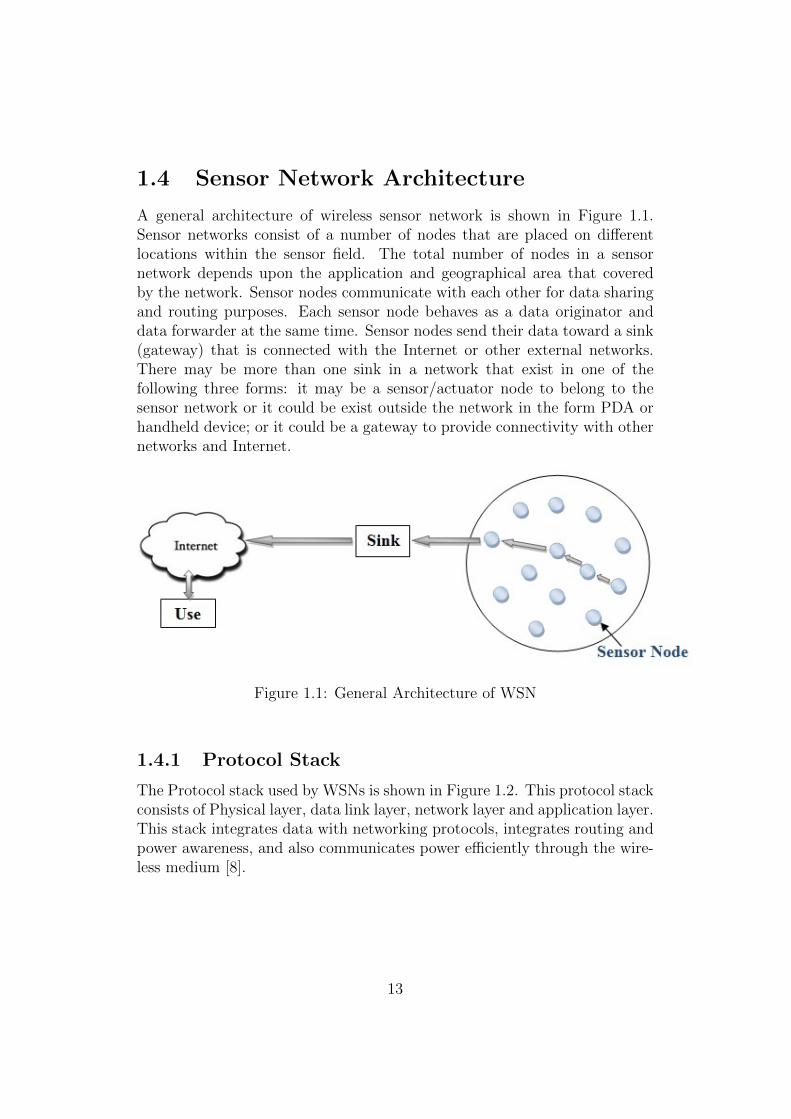
A general architecture of wireless sensor network is shown in Figure 1.1.Sensor networks consist of a number of nodes that are placed on differentlocations within the sensor field. The total number of nodes in a sensornetwork depends upon the application and geographical area that coveredby the network. Sensor nodes communicate with each other for data sharingand routing purposes. Each sensor node behaves as a data originator anddata forwarder at the same time. Sensor nodes send their data toward a sink(gateway) that is connected with the Internet or other external networks.There may be more than one sink in a network that exist in one of thefollowing three forms: it may be a sensor/actuator node to belong to thesensor network or it could be exist outside the network in the form PDA orhandheld device; or it could be a gateway to provide connectivity with othernetworks and Internet.

Figure 1.1: General Architecture of WSN

1.4.1 Protocol Stack

The Protocol stack used by WSNs is shown in Figure 1.2. This protocol stackconsists of Physical layer, data link layer, network layer and application layer.This stack integrates data with networking protocols, integrates routing andpower awareness, and also communicates power efficiently through the wire-less medium [8].

13

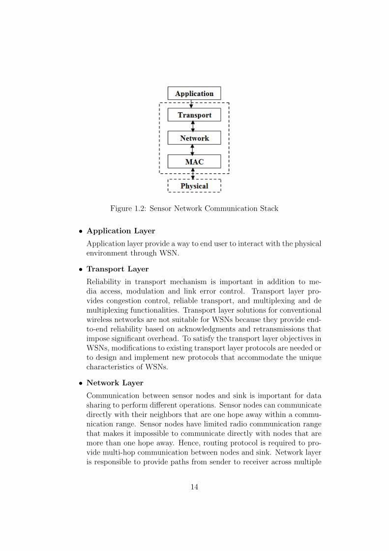
Figure 1.2: Sensor Network Communication Stack

• Application Layer

Application layer provide a way to end user to interact with the physicalenvironment through WSN.

• Transport Layer

Reliability in transport mechanism is important in addition to me-dia access, modulation and link error control. Transport layer pro-vides congestion control, reliable transport, and multiplexing and demultiplexing functionalities. Transport layer solutions for conventionalwireless networks are not suitable for WSNs because they provide end-to-end reliability based on acknowledgments and retransmissions thatimpose significant overhead. To satisfy the transport layer objectives inWSNs, modifications to existing transport layer protocols are needed orto design and implement new protocols that accommodate the uniquecharacteristics of WSNs.

• Network Layer

Communication between sensor nodes and sink is important for datasharing to perform different operations. Sensor nodes can communicatedirectly with their neighbors that are one hope away within a commu-nication range. Sensor nodes have limited radio communication rangethat makes it impossible to communicate directly with nodes that aremore than one hope away. Hence, routing protocol is required to pro-vide multi-hop communication between nodes and sink. Network layeris responsible to provide paths from sender to receiver across multiple

14

nodes. Network layer protocol must be power efficient, scalable, androbust.

• MAC Layer

Medium Access Control protocol is responsible to regulate the accessto a common medium between multiple nodes. It ensures the reliableconnections and data transmissions. In WSNs, MAC protocol providesthe creation of network infrastructure and share the energy, time, andfrequency resources between nodes [9]. Selected MAC scheme can in-fluence the efficiency of a sensor network in different ways includingenergy, delay and throughput. Collisions between nodes can affect thethroughput and also waste the energy.

1.4.2 ZigBee

ZigBee is a standard that defines protocols for low power and low data-ratewireless networking. ZigBee standard based devices operate on three differ-ent frequency bands at 868MHz, 915MHz, and 2.4 GHz. ZigBee is suitedfor battery operated devices with maximum 250 Kbps data rate. Devicesin ZigBee based applications stay in sleep mode to save the energy and arecapable of being operational for longer time periods. IEEE 802.15.4 wasadapted by ZigBee standard as Physical layer and MAC protocols. Devicesthat are compliant with ZigBee must be compliant with IEEE 802.15.4 stan-dard as well. ZigBee protocol stack is shown in Figure 4.1 where the bottomtwo layers are defined by IEEE 802.15.4 standard. ZigBee only defines theapplication, network, and security layers of the protocol [10].

1.4.3 IEEE 802.15.4

IEEE 802.15.4 is a low power, low data rate and low cost wireless protocolto serve home, industrial and medical applications. IEEE 802.15.4 focuseson the specification of the[hysical and the MAC layers for wireless sensornetworks. It is used with 6LoWPAN standard to build wireless embeddedInternet [10].

• IEEE 802.15.4 Physical Layer

The Physical layer provides data and management services interfac-ing to the PLME (Physical Layer Management Entity). Physical layerprovide the energy detection, channel selection, link quality indication,activation and deactivation of radio transceiver and clear channel as-sessment. Two PHY options are available based on frequency band.

15

Both options are based on direct sequence spread spectrum (DSSS)with data rate 250kbps at 2.4GHz, 40kbps at 915MHz and 20kbps at868MHz.

• IEEE 802.15.4 MAC Layer

The MAC layer provide data and management service and interface forthe MAC sublayer management entity (MLME) service access point(SAP). MAC layer provides channel access, beacon management, asso-ciation and disassociation, and acknowledged frame delivery. It worksin two different modes: beaconless and beacon-enabled mode. In bea-conless mode, unslotted CSMA-CA algorithm is used. In beacon-enabled mode, a superframe structure is used which is bounded bynetwork beacons and divided into 16 slots of equal sized. Beacon frameis sent in first slot of each superframe.

1.5 Node Architecture

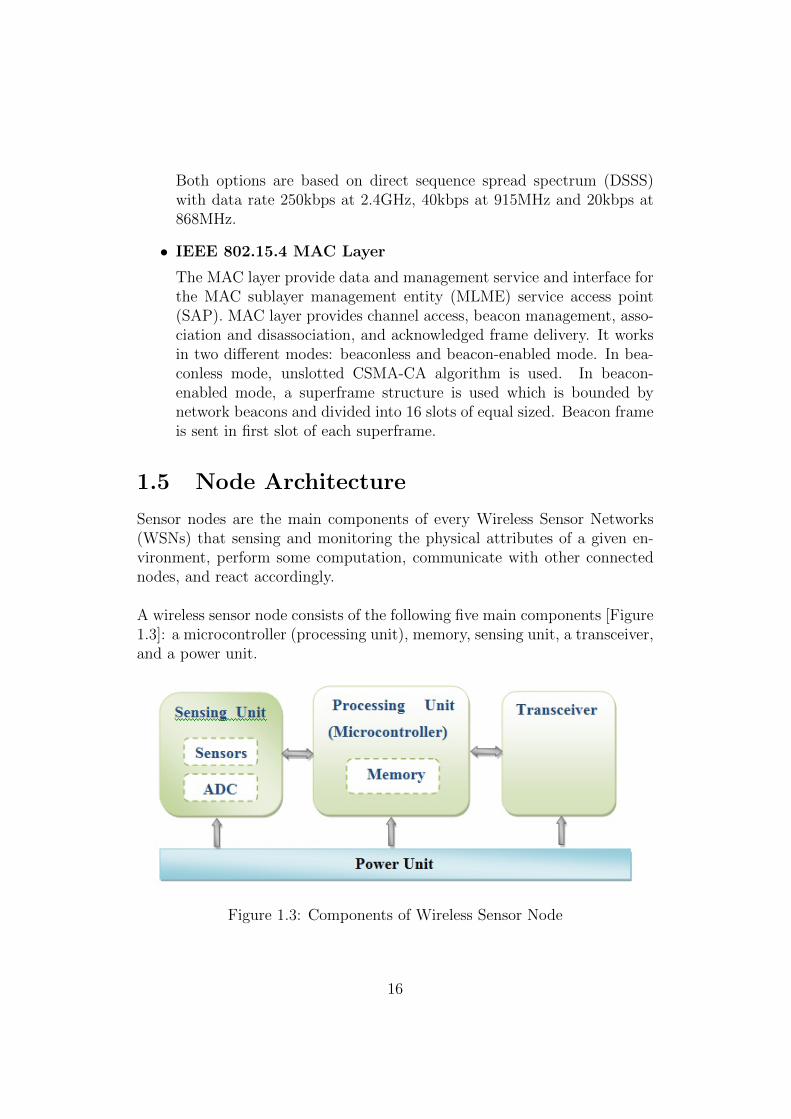
Sensor nodes are the main components of every Wireless Sensor Networks(WSNs) that sensing and monitoring the physical attributes of a given en-vironment, perform some computation, communicate with other connectednodes, and react accordingly.

A wireless sensor node consists of the following five main components [Figure1.3]: a microcontroller (processing unit), memory, sensing unit, a transceiver,and a power unit.

Figure 1.3: Components of Wireless Sensor Node

16

• Microcontroller

Microcontroller in a central processing and controlling unit of a sen-sor node that performs data processing and control the functionalityof other sensor nodes components. Instead of microcontrollers, thereare other alternatives available like digital signal processors, applicationspecific integrated circuit (ASIC), and desktop microprocessors. Micro-controllers are more flexible to connect other devices, programmable,and have less power consumption as compared to the other alternativesthat make them more suitable for embedded and sensor networks.

• Memory

Different options are available in memory for sensor nodes where on-chip, Read-Only memory (ROM), and flash memories are the mostrelevant options to store the program code. Random access memory(RAM) can be used to store sensor readings and packets from othernodes but its main disadvantage is that it is non-volatile by nature,which means that it loses its contents if power supply is interrupted.

• Sensing Unit

Sensing unit consist of one or more sensors that sense and measuressome physical parameters of the environment and send those measure-ments in the form of signals toward the microcontroller that processedthose measurements. Now a day, different types of sensors are availablelike thermal, seismic, visual, magnetic and acoustic. Sensors may beactive (without manipulation) or passive (using manipulation). Otherthan sensors, sensing unit also consist of some other sub componentsincluding transducer that converts energy from one form to anotherand analog-to-digital converter (ADC) that converts the output of asensor form continuous analog signal into a digital signal.

• Transceiver

Transceiver is responsible for the reception and transmission of data toother devices within the sensor network. Sensor nodes commonly usingRF (radio frequency) transceiver and PAN network technology such as802.15.4, or Bluetooth for communication.

• Power Source

Most of the sensor nodes are battery supported but some time alsosupported by power scavenging components for example, solar cells.Energy consumption is a most critical aspect in a sensor node design-ing. Sensor nodes consume power during sensing, communication, and

17

performing data processing. Sensor nodes consume more energy duringidle mode and also during sending and receiving the data.

18

Chapter 2

Routing Techniques forWireless Sensor Networks

2.1 Overview

In Wireless Sensor Networks (WSNs), sensor nodes communicate with eachother and also propagate their data toward a sink (gateway). There aretwo modes of communication one is single hop (direct) and another one ismulti-hop (indirect) communication. Single hop is feasible for small networkswhere all the nodes and a gateway are close to each other. Multi-hop mode ofcommunication is suitable for larger networks, where large number of nodesexists and covering large geographical area. In multi-hop WSNs, sender cansend data by using intermediate nodes which can route the data towardsthe receiver. Multi-hop communication is possible by routing which is theprocess of finding the best paths from a sender to a receiver (Sink). Differenttypes of routing protocols are used to find the best paths from a sender toa receiver and maintain routing tables on IP routers by using different kindsof algorithms, and metrics.

This chapter covers the main challenges and metrics of routing in WSNs.Moreover, the main categories and strategies of routing protocols are de-scribed in detail. Finally, last section is devoted to IETF working groupROLL (Routing over Low power and Lossy networks) that is working towardthe development of RPL routing protocol for WSN.

19

2.2 Challenges

Finding optimal routing solutions in WSNs is a challenging task becauseof lossy wireless links with limited bandwidth and most important are theconstraints over sensor nodes like limited energy supply, low memory andprocessing capability. Because of these challenges and constraints over sensornodes, traditional routing protocols developed for wired and wireless ad hocnetworks are not suitable for WSNs. In the following section, we describesome of the routing challenges that affect the whole routing process in WSNs.

• Energy Consumption

Because of limited energy resources of sensors nodes, energy in the mainconcern in the design and development of routing protocol for sensornetworks. Sensor nodes deliver their data in energy-efficient mannerwithout losing the accuracy of routed data. Because of this constraintover energy, most of the conventional routing metrics like shortest pathare not suitable for WSNs [11].

• Network Dynamics

Sensor nodes in WSNs are usually assumed to be stationary. However,mobility of both sensor nodes and base stations can affect the routesand overall communication structure. Route stability is an importantissue, in addition to energy and other aspects. So the routing protocolshould be adaptive to dynamic changes in the network topology.

• Scalability

Some WSN applications demanding a large number of sensor nodesdeployments that cover larger area to observe the physical phenomena.With such large number of nodes make it impractical to obtain topologyinformation from each node in the network. Hence, routing protocolshould provide scalability that operate with limited information andalso limit the local information exchange in order to improve the energyefficiency.

• Robustness

In WSNs, routing is performed by routing protocols that are operatedon sensor nodes instead of dedicated routers. These sensor nodes con-sist of low cost hardware as compared to dedicated routers that maycause of unexpected failures in sensor nodes. Sometimes these failuresmake the nodes non-operational. Therefore, routing protocol shouldprovide robustness to sensor node failures.

20

• Node deployment

Node deployment in sensor networks can be either randomized or de-terministic which is dependent on the required application. In deter-ministic approach of deployment, all the sensor nodes are placed onmanually predefined locations and data is routed through paths thatare also pre-determined. However, in randomized approach, all the sen-sor nodes placed randomly in ad hoc manner. Initially, sensor nodeshave no information about network topology. Routing protocol shouldprovide topology information such that the neighbors of each node arediscovered and routing decisions are made accordingly.

2.3 Metrics

Routing protocols decision about best route selection among multiple routesis based on the type of route metric. Commonly used metrics for routing arehop count, energy, load, Expected Transmission Count (ETX), and ExpectedTransmission Time (ETT). In this section, we discuss in brief some of thesecommonly used routing metrics in WSNs.

• Minimum Hop Count

Number of hop count is a most common metric used in routing proto-cols, where routing protocol find the path from sender to receiver thathave minimum number of hops (shortest hop). In this route selectionmetric, routing protocol never consider the link cost and select the paththat involved the smallest number of forwarding nodes and minimizesthe total data propagation cost from sender to receiver. Minimum-hopbased routing protocol provide no optimal route in terms of congestion,delay, and energy because it never consider the resource availability oneach node.

• Energy

The most critical resource in LLNs is available energy of sensor nodesthat make it more challenging to propagate a single packet from sourceto a destination by using minimum energy. Sometimes a node withminimum available energy is avoided to select as a router which mayresult in non optimal or longer paths. To maximize the lifetime of awhole network depends upon the equally distribution of energy on allnetwork nodes.

21

• Expected Transmission Count (ETX)

ETX, proposed by de Couto et al (2003), is defined as the expectednumber of MAC layer transmissions necessary to successfully deliveringa packet through a wireless link. The weight of a path is defined as thesummation of the ETX of all links along the path. ETX is a routingmetric that ensure easy calculation of minimum weight paths and loopfree routing under all routing protocols. ETX never consider the energyconsumption of devices.

• Expected Transmission Time (ETT)

Expected transmission time is an estimation of time cost of sending apacket successfully through a MAC layer [12]. It takes the link band-width into account and commonly used to express latency.

2.4 Classification of Routing Protocols

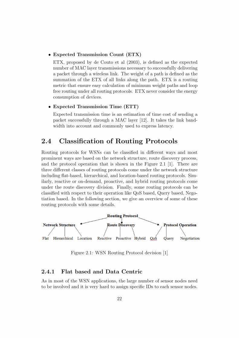
Routing protocols for WSNs can be classified in different ways and mostprominent ways are based on the network structure, route discovery process,and the protocol operation that is shown in the Figure 2.1 [1]. There arethree different classes of routing protocols come under the network structureincluding flat-based, hierarchical, and location-based routing protocols. Sim-ilarly, reactive or on-demand, proactive, and hybrid routing protocols comeunder the route discovery division. Finally, some routing protocols can beclassified with respect to their operation like QoS based, Query based, Nego-tiation based. In the following section, we give an overview of some of theserouting protocols with some details.

Figure 2.1: WSN Routing Protocol devision [1]

2.4.1 Flat based and Data Centric

As in most of the WSN applications, the large number of sensor nodes needto be involved and it is very hard to assign specific IDs to each sensor nodes.

22

Therefore, routing protocols that are based on unique IDs or addresses arenot suitable for WSNs. To provide the solution for this problem, data cen-tric routing protocols have been proposed. In data centric routing tech-niques, sensor nodes have less importance than the information they generate.Therefore, data centric routing protocols based on attribute naming, insteadof individual node IDs. The Sensor protocols for Information via Negotia-tion (SPIN), flooding, rumor routing, directed diffusion, and gradient-basedrouting are few examples of routing protocols that may apply data-centrictechniques. In the following section, we provide an overview of some of thesedata-centric based routing protocols in flat-based networks. In flat basednetworks, all the sensor nodes are considered equally with respect to theirrole and functionality.

• Flooding

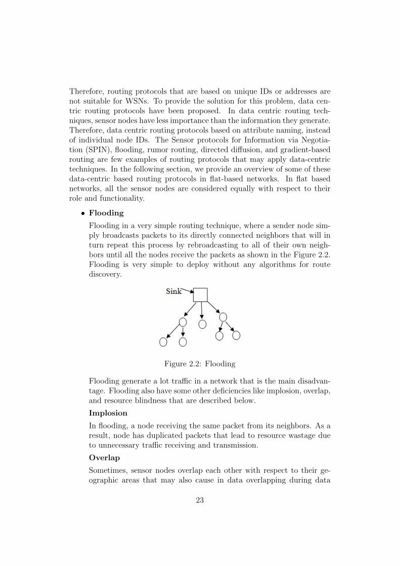
Flooding in a very simple routing technique, where a sender node sim-ply broadcasts packets to its directly connected neighbors that will inturn repeat this process by rebroadcasting to all of their own neigh-bors until all the nodes receive the packets as shown in the Figure 2.2.Flooding is very simple to deploy without any algorithms for routediscovery.

Figure 2.2: Flooding

Flooding generate a lot traffic in a network that is the main disadvan-tage. Flooding also have some other deficiencies like implosion, overlap,and resource blindness that are described below.

Implosion

In flooding, a node receiving the same packet from its neighbors. As aresult, node has duplicated packets that lead to resource wastage dueto unnecessary traffic receiving and transmission.

Overlap

Sometimes, sensor nodes overlap each other with respect to their ge-ographic areas that may also cause in data overlapping during data

23

collection and dissemination to neighbor nodes. Sending and receivingsame data will lead to resource wastage. Overlap problem is difficultto address as compared to implosion.

Resource blindness

Flooding never consider the resource constraints of individual nodes.As each node has limited energy resource that must be consumed effi-ciently but flooding protocol does not take into account the availableenergy resources of individual nodes.

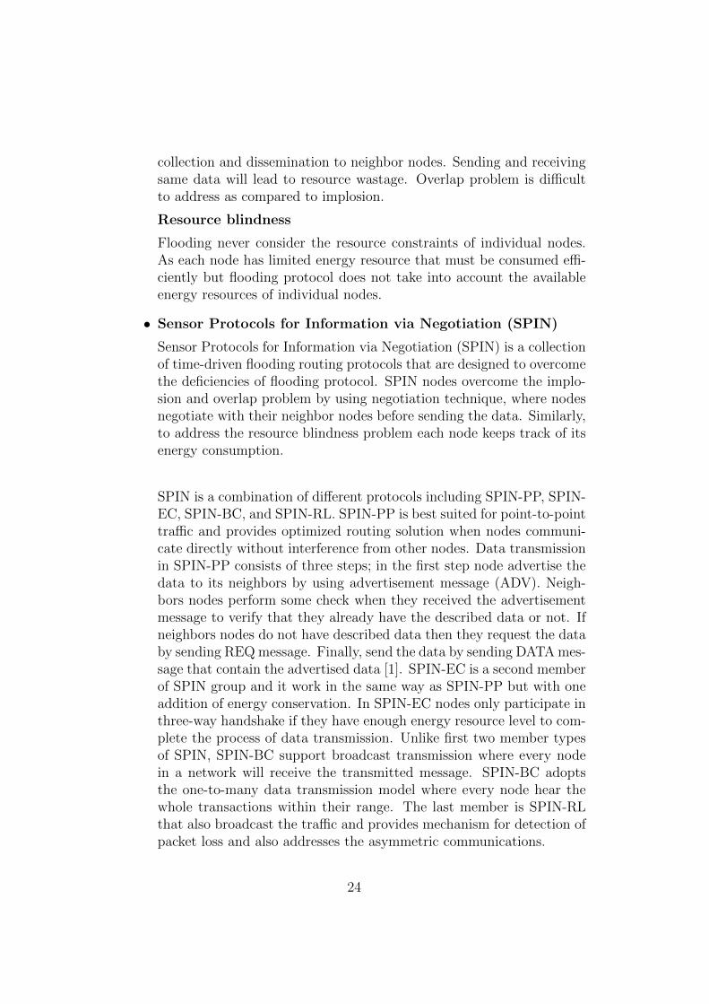
• Sensor Protocols for Information via Negotiation (SPIN)

Sensor Protocols for Information via Negotiation (SPIN) is a collectionof time-driven flooding routing protocols that are designed to overcomethe deficiencies of flooding protocol. SPIN nodes overcome the implo-sion and overlap problem by using negotiation technique, where nodesnegotiate with their neighbor nodes before sending the data. Similarly,to address the resource blindness problem each node keeps track of itsenergy consumption.

SPIN is a combination of different protocols including SPIN-PP, SPIN-EC, SPIN-BC, and SPIN-RL. SPIN-PP is best suited for point-to-pointtraffic and provides optimized routing solution when nodes communi-cate directly without interference from other nodes. Data transmissionin SPIN-PP consists of three steps; in the first step node advertise thedata to its neighbors by using advertisement message (ADV). Neigh-bors nodes perform some check when they received the advertisementmessage to verify that they already have the described data or not. Ifneighbors nodes do not have described data then they request the databy sending REQ message. Finally, send the data by sending DATA mes-sage that contain the advertised data [1]. SPIN-EC is a second memberof SPIN group and it work in the same way as SPIN-PP but with oneaddition of energy conservation. In SPIN-EC nodes only participate inthree-way handshake if they have enough energy resource level to com-plete the process of data transmission. Unlike first two member typesof SPIN, SPIN-BC support broadcast transmission where every nodein a network will receive the transmitted message. SPIN-BC adoptsthe one-to-many data transmission model where every node hear thewhole transactions within their range. The last member is SPIN-RLthat also broadcast the traffic and provides mechanism for detection ofpacket loss and also addresses the asymmetric communications.

24

• Directed Diffusion

Directed diffusion is a data centric protocol in which data generated bynodes is named by attribute-value pairs. A node sending request fornamed data and matching data with the interest is then drawn towardsthe requested node [13]. Data is transformed from source to destinationthrough intermediate nodes that can also cache the data.

2.4.2 Hierarchical

The data-centric routing protocols have some scalability and efficiency prob-lems, hence hierarchical routing protocols were proposed to overcome theseproblems. In hierarchical routing technique, nodes are grouped to form thecluster where all the nodes communicate only with the leader node (clus-ter head) within that cluster as shown in the Figure 2.3 [1]. These clusternodes that have more power and less energy constraint, are responsible forpropagation of sensor data toward the sink.

Hierarchical routing techniques also have some design and operation chal-lenges like cluster formation, and cluster head selection. Some of the hierar-chical based routing protocols are low energy adaptive clustering hierarchy(LEACH), threshold sensitive energy efficient sensor network (TEEN), powerefficient gathering in sensor information systems (PEGSIS), and adaptivethreshold sensitive energy efficient sensor network (APTEEN) [14].

• LEACH

Low Energy Adaptive Clustering Hierarchy (LEACH) is an adaptiveclustering and self organizing protocol. LEACH minimizes the energyconsumption by forming the clusters and uniformly distributes energyconsumption at every node in the network [14].

2.4.3 Location Based

Location based routing also known as geographic routing is a routing tech-nique that based on geographic information of sensor nodes instead of topo-logical connectivity information. In this routing technique, sensor nodes sendtheir unicast data directly to a single destination, which in identified by its lo-cation. Sensor nodes obtain the location information of destination by using

25

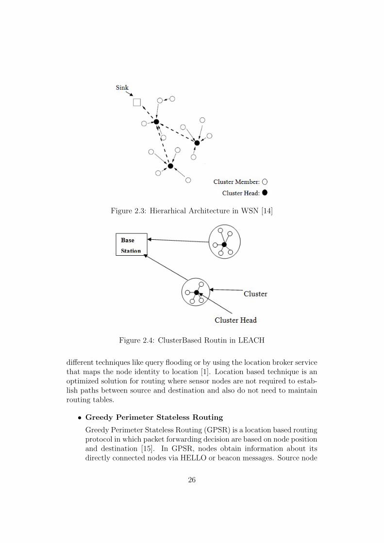
Figure 2.3: Hierarhical Architecture in WSN [14]

Figure 2.4: ClusterBased Routin in LEACH

different techniques like query flooding or by using the location broker servicethat maps the node identity to location [1]. Location based technique is anoptimized solution for routing where sensor nodes are not required to estab-lish paths between source and destination and also do not need to maintainrouting tables.

• Greedy Perimeter Stateless Routing

Greedy Perimeter Stateless Routing (GPSR) is a location based routingprotocol in which packet forwarding decision are based on node positionand destination [15]. In GPSR, nodes obtain information about itsdirectly connected nodes via HELLO or beacon messages. Source node

26

mark the sending data with the location of the receiving node andrelay a packet to its immediate neighbor that make a locally forwardingdecision and handle the data to neighbor that is geographically closeto the destination. Every node from source to destination make localforwarding decision and move data closer to the destination hop byhop, until the destination is reached.

2.4.4 QoS

In some WSN applications, Quality-of-Service related metrics like delay, jit-ter, and throughput have same importance as energy consumption. Similarly,some routing protocols goal is to fulfill some QoS metrics while finding fea-sible paths between sender and receiver. To fulfill the QoS requirements inWSNs in a challenging task because of scarce resources like energy, dynamictopologies changes, and lack of centralized control. The following sectionprovides an overview of QoS based routing protocols for sensor networks.

• Sequential Assignment Routing

Sequential Assignment Routing (SAR) is a multipath routing approachthat explicitly considers the QoS metrics. SAR creates multiple treesthat are rooted from one hope neighbor nodes of the sink. Trees growoutward from a sink while avoiding those nodes that have low QoS andenergy. SAR selection for route based on QoS metric, packet prioritylevel, and energy. Every node in a network is a part of multiple treesand it can select multiple routes toward the sink. Multiple paths avail-ability provides fault tolerance and fast recovery from broken paths.In large networks, multiple trees establishment and maintaining areexpensive.

• SPEED

SPEED is a QoS based routing protocol that provides real time uni-cast, multicast, and anycast communication services. Nodes in SPEEDprotocol relies on location information of sensor nodes instead of rout-ing tables, therefore SPEED is also a location based stateless routingprotocol [16]. SPEED protocol based on several different componentsto make sure speed guarantees to the packets. SPEED is scalable andefficient protocol suited for highly dense environments where large num-bers of nodes with limited resources are deployed.

27

28

Chapter 3

RPL Routing Protocol

3.1 ROLL Working Group

The ROLL (Routing Over Low Power and Lossy network) is a working groupcreated by IETF for the purpose of to analyze the routing requirements ofapplications including industrial automation [17], home and building automa-tion [18, 19], and smart grid. The main objective of ROLL working groupwas to design and develop the routing solutions for IP-based Low power andLossy Networks (LLN) that have support of a variety of link layers [20]. ALLN is made up of embedded devices that have limited memory, low energy(battery power), and low processing capability. In LLNs, links are lossy andmay become unstable for short time of period that may cause by a numberof reasons for example interference. LLNs include a wide range of link layertechnologies, including Bluetooth, IEEE 802.15.4, Power line communica-tion (PLC), and low-power Wi-Fi. LLN have distinguished characteristicsthat are specified in [2]. The result of ROLL working group was the RPL(Routing Protocol for LLN) specification, along with specifications on rout-ing metrics, security, and objective functions. Until now ROLL group hasspecified several documents on the routing requirements for different appli-cations of WSN like home and building automation, industrial applications,and urban deployments.

3.2 RPL Protocol Overview

RPL is an IPv6 based distance vector routing protocol for low power andlossy networks (LLNs) [21]. RPL allows routing across multiple types of linklayers. RPL is a modular routing protocol means that the core of the RPLprotocol is the intersection of the application-specific requirements that are

29

spelled out in [17, 18, and 19]. RPL is a gradient based routing protocol thatbuilds the graph known as Directed Acyclic Graph (DAG) by using a set ofmetrics/constraints and an objective function. DAG grounded at the pointknown as Low power and lossy network Border Router (LBR). Each nodehas an assigned rank that incremented as the node go away from the LBR.Packet forwarding toward LBR is consisting in picking the neighbor nodewith lowest rank [22]. Whole topology graph is divided into multiple RPLInstances that are uniquely identified by RPLInstanceID. RPL Instance is aset of multiple DODAGs (Destination Oriented DAG) and each DODAG isuniquely identified by DODAGID.

3.2.1 Graph Building Process

RPL routing protocol convert the physical topology into logical by build-ing a Directed Acyclic Graph (DAG). Whole graph consists of at least oneinstance. Within an instance, whole topology is divided into multiple Desti-nation Oriented DAGs (DODAGs) in order to provide a greater scalability.DODAG is a set of vertices that are connected by directed edges with nocycles. Each DODAG is optimized to provide different QoS requirements[21]. DODAGs start from the root node that advertises the graph relatedinformation to other nodes. Root (SINK) node sends information in the formof ICMPv6 control messages known as DIO (DODAG Information Object).Nodes that receive the messages will process these messages and make deci-sion whether to join the graph or not and also forward the DIO messages toit’s neighboring nodes. This process continuous such that the DAG topologyis built from the sink node toward edges nodes as shown in figure 3.1. Everynode that joins the graph has a route toward the root of the graph. Nodesthat join the graph act in one of the two ways, if node acts as a router it ad-vertise the graph information to its neighbors. Otherwise node acts as a leafnode and does not send the DIO messages. All the neighboring peers repeatthis whole process and build the graph edges. All the leaf nodes send datapackets hop-by-hop towards root (Upward) and represents a Multipoint-to-Point (MP2P) model. Leaf nodes have redundant paths towards the SINKnode that is a main requirement of LLNs.

3.2.2 Types of RPL Messages

RPL build whole topology graph by using three different ICMPv6 based con-trol messages: the DODAG Information Object (DIO), the DODAG Destina-tion Advertisement Object (DAO), and the DODAG Information Solicitationmessage (DIS). All these three messages using the same ICMPv6 code point.

30

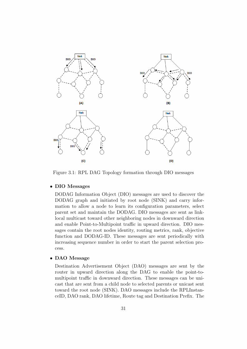
Figure 3.1: RPL DAG Topology formation through DIO messages

• DIO Messages

DODAG Information Object (DIO) messages are used to discover theDODAG graph and initiated by root node (SINK) and carry infor-mation to allow a node to learn its configuration parameters, selectparent set and maintain the DODAG. DIO messages are sent as link-local multicast toward other neighboring nodes in downward directionand enable Point-to-Multipoint traffic in upward direction. DIO mes-sages contain the root nodes identity, routing metrics, rank, objectivefunction and DODAG-ID. These messages are sent periodically withincreasing sequence number in order to start the parent selection pro-cess.

• DAO Message

Destination Advertisement Object (DAO) messages are sent by therouter in upward direction along the DAG to enable the point-to-multipoint traffic in downward direction. These messages can be uni-cast that are sent from a child node to selected parents or unicast senttoward the root node (SINK). DAO messages include the RPLInstan-ceID, DAO rank, DAO lifetime, Route tag and Destination Prefix. The

31

most significant information is Reverse Route Stack that is carried bythese messages.

• DIS Message

Destination Information Solicitation (DIS) messages are used to trig-ger a DIO transmission from a RPL node. These messages have nobody and are sending by node to join a network. As an alternativeto wait to receive a DIO message, a node broadcast a DIS message toneighborhood and solicits DIOs from RPL neighboring nodes.

3.2.3 Objective Function

Objective Function is used in RPL to construct the DODAG and define hownodes in RPL select the routes within an instance. RPL define the wholetopology by constructing DODAGs with in instances and each instance is as-sociated with a specialized objective function. Objective Function combinesthe metrics and constraints to find the best path. For example, the objectivefunction finds the path that has minimum delay and that path never tra-verse a battery-operated node. In this example, path with minimum delay isrepresenting the metric and non-battery operated nodes are representing theconstraint. Each Objective Function is identified by Objective Code Point(OCP) in a DIO configuration option. Objective function is also used todefine the rank of a node which is a nodes distance from a DODAG rootnode. RPL main specification has no default objective function. Therefore,Objective Function 0 (OF0) is designed as a default function that is com-mon to all implementations and provide interoperability between differentimplementations.

3.2.4 Trickle Timer

Trickle Timer is used to control the sending of DIO and DAO messages.Trickle timer is based on dynamic timers that govern the transmission ofRPL control messages in energy efficient, and scalable manner and also toreduce redundant messages. Trickle timer control the inconsistency and avoidredundant transmissions of DIO messages. In case of instability in DODAG,trickle time interval become shorter and control messages are sent frequentlyto stabilize the DODAG. Similarly, when DODAG become stabilize controlmessages are sent less frequent to reduce the control plane overhead.

32

3.3 RPL Traffic Pattern

RPL support three different traffic patterns: Multipoint-to-Point (MP2P),Point-to-Multipoint (P2MP), and Point-to-Point that will be discussed inmore detail in the following section.

3.3.1 Multipoint-to-Point

RPL enable the Multipoint-to-Point (MPTP) traffic in upward direction bysending DIO messages from the DODAG roots down toward the leaf nodes.DIO messages are used to form and maintained the DODAGs. A node joinsthe DODAG and discovers the neighboring nodes that are already part of theDODAG and built a parent set. The parent set is collections of the candidateneighbor set that are reachable via link-local multicast. Any node with lowerrank as compared to the node itself is considered as a candidate of parent set.A preferred parent is selected form the parent set to used as a next hop forupward routes. Multipoint-to-Point communication is a most dominant formof traffic in RPL. Upward routing process is of great importance to build theDODAG that is based on the Distributed Algorithm that involves selectionand configuration of some nodes as DODAG Roots.

3.3.2 Point-to-Multipont

RPL enable the Point-to-Multipoint traffic and provide the routes down theDODAG to reach the certain non DODAG root nodes in downward direction.Point-to-Multipoint traffic is accomplished by sending the DAO messages inupward direction toward the DODAG Root.

The downward routes are maintained by nodes in two modes know as storingand non-storing. In storing mode, each non-root node in a graph need to storeprefixes information that they received in the form of DAO messages fromneighbor nodes. Some nodes in the network have constraints over memoryand may be incapable of storing routing entries for downward. These nodesare non-storing nodes and in this non-storing mode only the DODAG rootstore the routes and responsible for all downward routing.

3.3.3 Point-to-Point

Similarly, some time traffic flow downward from intermediate or root node toleaf node. Destination Advertisement Object (DAO) messages are sending by

33

the nodes to established the downward routes. In RPL, nodes also send point-to-point traffic, where a node send its traffic upward to a common ancestorpoint at which it is forwarded in the downward to the destination. Point-to-Point routing can also be supported by storing and non-storing modes.

34

Chapter 4

Experiment Setup

This Chapter is about the experimental setup in a real word testbed environ-ment. This chapter provides the details about software (Contiki OS, ContikiCollect) and hardware (Tmote Sky) components that are used to experimen-tally evaluate the performance and route stability of RPL protocol.

4.1 Contiki Operating System

Contiki is an open source portable operating system that is specifically de-signed for small sensor networks and embedded devices. It was designed anddeveloped by Swedish Institute of Computer Science (SICS) with the coop-eration of group of developers from academia and industry. Contiki providesthe TCP/IP communication both for IPv4 and IPv6 by using uIP stackand has low memory requirements that needs only 2 kilobytes of RAM forthe configuration and 40 kilobytes of ROM for the whole system includinggraphical user interface [23].

Contiki provides a number of features including, protocol-independent radionetworking, IPv6 stack with power-efficient radio mechanism, ContikiMACthat allow battery-operated devices and routers, cross-layer network simu-lator COOJA with MSP Emulator that makes software development anddebugging easier and faster, software based power profiling mechanism thatmonitor the energy consumption of each node to reduce and control the powerconsumption, and recently included a networked shell and the memory effi-cient flash-based power profiling [24].

Contiki is developed by using C programming language and also provideC based programming development environment. Contiki provides Instant

35

Contiki, a Linux based software environment that contains all the necessarytools and compilers for software development in Contiki. Instant Contikiruns in a virtual environment within VMware player.

The latest version of Contiki is 2.5 which bring new features and improve-ments over previous releases, such as IETF RPL routing protocol implemen-tation, Contiki MAC radio duty cycling protocol, IETF CoRE CoAP protocolimplementation, Contiki collect address-free data collection protocol, and anumber of new platforms. In the next sub section, we will give some overviewabout the Contiki protocol stacks and ContikiRPL.

4.1.1 uIP and Rime Protocol Stacks

Contiki contains the uIP and Rime communication stacks. uIP is a smalllight-weight TCP/IP stack with TCP, UDP, IP and ARP protocols. uIPprovides Internet communication abilities to Contiki and make it possi-ble to communicate by using the TCP/IP protocol suite on a 8-bit micro-controllers. uIP is written in C programming language and its implemen-tation consider only the minimal set of features that are needed for a fullTCP/IP stack. uIP provides architecture independent functionalities andsome architecture specific functions. uIP includes the memory managementfunctionalities to better handle the memory as RAM is the most scarce re-source on the architectures on which uIP is intended. uIP also provides APIsto enable the application program to interact with the TCP/IP stack [25].

Rime is designed for low-power radios and it simplifies the implementation ofsensor network protocols. Rime stack is organized in very simple layers whereeach layer adds its own header to outgoing messages. Rime stack providesboth single-hop and multi-hop communication. In multi-hop communication,Rime do not specify how packets routed from source to destination. Thenext-hop foewarding procedure is left to upper layer protocols.

4.1.2 ContikiRPL

ContikiRPL is an implementation of the RPL protocol that separates pro-tocol logic, objective functions, from message construction and parsing intodifferent modules. The ContikiRPL logic module maintains and manages theDAG graph information, build and maintains a parents set for each node ina network, validate the RPL messages according to RPL specification, andcommunicate with objective functions. ContikiRPL create the forwarding ta-bles for uIPv6 and does not involve in forwarding decisions that only perform

36

by uIPv6. The implementation of ContikiRPL works in COOJA simulatorwithout any modification of platform [26].

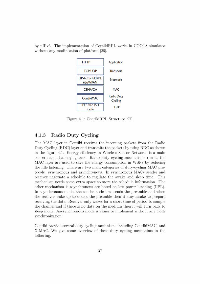
Figure 4.1: ContikiRPL Structure [27].

4.1.3 Radio Duty Cycling

The MAC layer in Contiki receives the incoming packets from the RadioDuty Cycling (RDC) layer and transmits the packets by using RDC as shownin the figure 4.1. Energy efficiency in Wireless Sensor Networks is a mainconcern and challenging task. Radio duty cycling mechanisms run at theMAC layer are used to save the energy consumption in WSNs by reducingthe idle listening. There are two main categories of duty-cycling MAC pro-tocols: synchronous and asynchronous. In synchronous MACs sender andreceiver negotiate a schedule to regulate the awake and sleep time. Thismechanism needs some extra space to store the schedule information. Theother mechanism is asynchronous are based on low power listening (LPL).In asynchronous mode, the sender node first sends the preamble and whenthe receiver wake up to detect the preamble then it stay awake to preparereceiving the data. Receiver only wakes for a short time of period to samplethe channel and if there is no data on the medium then it will turn back tosleep mode. Asysynchronous mode is easier to implement without any clocksynchronization.

Contiki provide several duty cycling mechnisms including ContikiMAC, andX-MAC. We give some overview of these duty cycling mechanims in thefollowing.

37

• ContikiMAC

ContikiMAC is a newly implemented duty cycling mechanism in Con-tiki 2.5. It is a default mechanism in Contiki 2.5 and it uses periodicalwake-ups to listen for packet transmissions from neighbors. In Contiki-MAC, nodes stay in sleep mode most of the time and in case of packettransmission detection, the receiver wakes up to receive the next packetand then sends a link layer acknowledgement. In order to send a packetsuccessfully, the sender sends the same packet repeatedly until the linklayer acknowledgment is received.

ContikiMAC is very simple asynchronous mechanism with no signal-ing messages and without any additional packet headers. It is powerefficient and relies on different timing between transmissions. Contiki-MAC uses the Clear Channel Assessment (CCA) in order to check theradio activity on the channel [28].

• X-MAC

X-MAC is an older mechanism that is less power-efficient than Contiki-MAC but has less stringent timing requirements. In order to reduce theenergy consumption, X-MAC mechanism employs a shortened pream-ble approach and an enhanced version of low power listening that re-tains the low power communication, simplicity and a recouping of trans-mitter and receiver sleep schedules. Nodes that want to send data, justturn on their radios and start to sends short preambles (strobes) un-til they receive an acknowledgement. Non-sending nodes periodicallywake ups for short listening period after a sleep time in order to checkthe channel for strobes.

X-MAC implementation in Contiki has some parameters that controlthe listening and sleeping time of nodes. Ontime parameter determinesthe time that a receiver listens for strobes and offtime is for sleepingtime between waking up to listening for strobes. Strobe-time is the timeduration for a sender to transmit strobes until it receives acknowledg-ment from the receiver side.

38

4.2 Setup of the Experiment

In order to analyze the performance and route stability of RPL, we haveconsidered a wide range of configuration settings.

4.2.1 Testbed

For experiments, we used a deployed indoor testbed with 15 number of Tmotesky motes distributed over single floor in the university building as shown inFig 4.2. One of the 15 nodes is configured as the root of the routing while theremaining nodes operated as sender to send the generated packets toward theroot node. All the nodes are running the Contiki operating system version2.5 and form a routing tree by using RPL routing protocol. The placementof the nodes is fixed. We have experiments with a single root node for eachconfiguration.

Figure 4.2: Tmote Sky testbed topology used for the experiments. The Sinknode is connected with the computer to collect and print the data on thecomputer.

Evaluations are performed over two different MAC layer Radio duty cyclingprotocols. All sender nodes send the data packets of size 87 bytes toward theSink. All the experiments run for about 15 minutes. We performed multipleexperiments for each configuration and with different time intervals betweenpackets send by the nodes toward sink. All the experiments are perform byusing the radio channel 24.

When the network boots up, the pre configured root node starts the Con-tikiRPL operations by sending DIO messages and sender nodes start to gen-

39

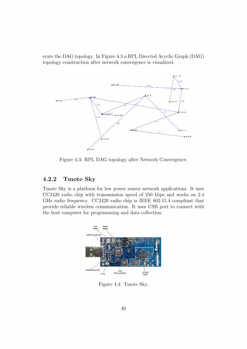
erate the DAG topology. In Figure 4.3 a RPL Directed Acyclic Graph (DAG)topology construction after network convergence is visualized.

Figure 4.3: RPL DAG topology after Network Convergence.

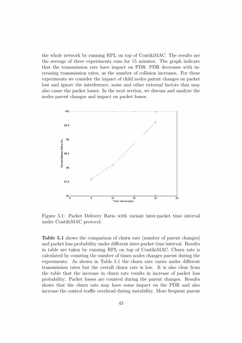
4.2.2 Tmote Sky

Tmote Sky is a platform for low power sensor network applications. It usesCC2420 radio chip with transmission speed of 250 kbps and works on 2.4GHz radio frequency. CC2420 radio chip is IEEE 802.15.4 compliant thatprovide reliable wireless communication. It uses USB port to connect withthe host computer for programming and data collection.

Figure 4.4: Tmote Sky.

40

41

Chapter 5

Results

This chapter presents the experimental evaluation study of RPL using mea-surements collected from the testbed that is described in Chapter 4. RPLin its initial implementation rely on Expected Transmission Count metric(ETX) to select the path that provide with minimum ETX value. ETX is amaximum number of retransmissions that are needed to send the individualpacket successfully toward next hop or Sink. Power is the scarce sourcein WSN. Nodes select the path with minimum ETX value which meansless number of retransmissions and therefore low power consumption. Weevaluate the RPL performance and parent changes on top of two differentMAC layer radio duty cycling mechanisms ContikiMAC and X-MAC. Exper-iments are performed with different inter-packet time interval and transmis-sion power in order to check the effect of these factors on RPL performanceand stability. These factors will be analyzed by using experimental data thatis obtained from the testbed.

RPL performance and stability on top of ContikiMAC Protocol:

A first set of experiments is performed by running RPL on top ContikiMACradio duty cycling protocol. Experiments are carried out with different inter-packet time interval including 20 sec, 10 sec, and 5 sec in order to investigatehow the performance and network stability are affected depending on thenetwork load. Experiment runs for three times with with each interval anda of duration of 15 minutes. Each node send the data packet of size 87 bytestowards sink. The channel check rate is set to 16Hz with transmission power(Tx) set to 31 (0 dBm). Other parameters are kept constant with defaultconfiguration of ContikiMAC protocol.

Figure 5.1 shows the average end-to-end Packet Delivery Ratio (PDR) of

42

the whole network by running RPL on top of ContikiMAC. The results arethe average of three experiments runs for 15 minutes. The graph indicatethat the transmission rate have impact on PDR. PDR decreases with in-creasing transmission rates, as the number of collision increases. For theseexperiments we consider the impact of child nodes parent changes on packetlost and ignore the interference, noise and other external factors that mayalso cause the packet losses. In the next section, we discuss and analyze thenodes parent changes and impact on packet losses.

Figure 5.1: Packet Delivery Ratio with variant inter-packet time intervalunder ContikiMAC protocol.

Table 5.1 shows the comparison of churn rate (number of parent changes)and packet loss probability under different inter-packet time interval. Resultsin table are taken by running RPL on top of ContikiMAC. Churn rate iscalculated by counting the number of times nodes changes parent during theexperiments. As shown in Table 5.1 the churn rate varies under differenttransmission rates but the overall churn rate is low. It is also clear fromthe table that the increase in churn rate results in increase of packet lossprobability. Packet losses are counted during the parent changes. Resultsshows that the churn rate may have some impact on the PDR and alsoincrease the control traffic overhead during instability. More frequent parent

43

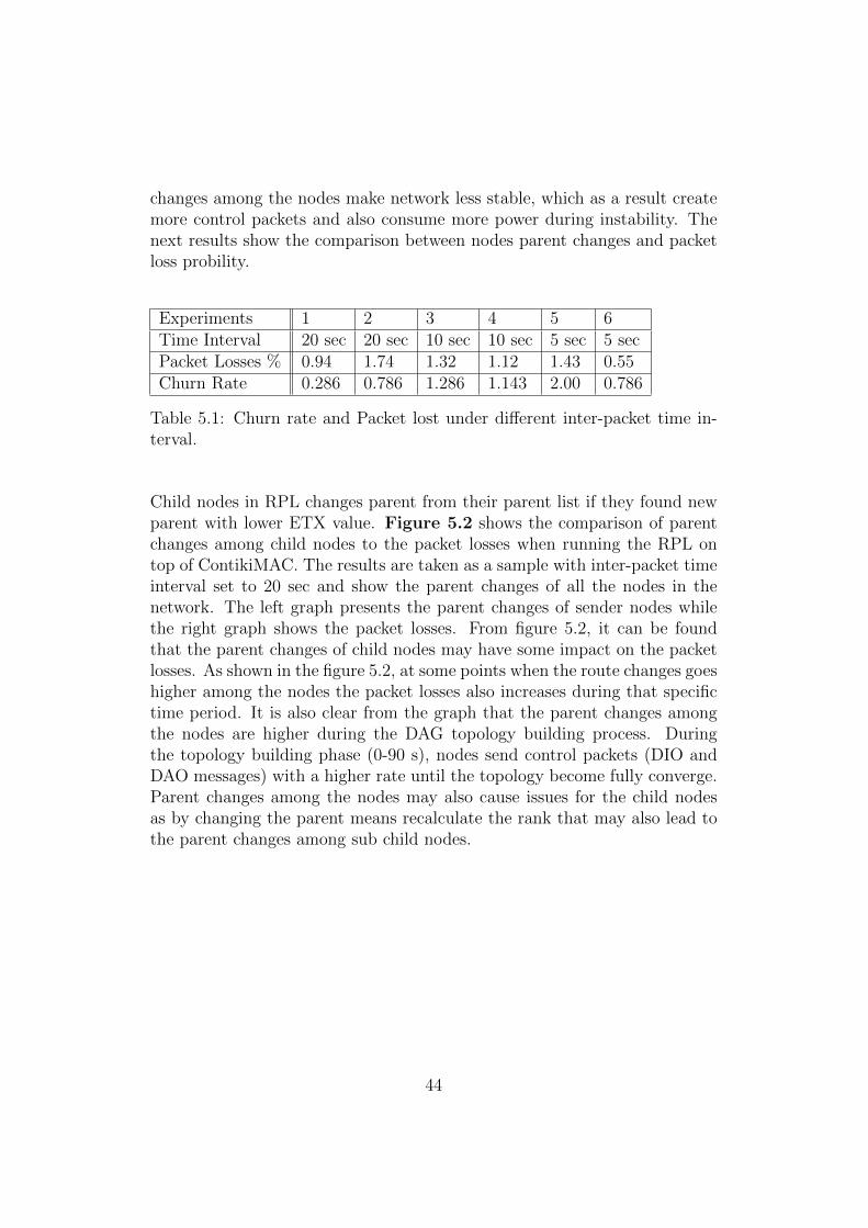
changes among the nodes make network less stable, which as a result createmore control packets and also consume more power during instability. Thenext results show the comparison between nodes parent changes and packetloss probility.

Experiments 1 2 3 4 5 6Time Interval 20 sec 20 sec 10 sec 10 sec 5 sec 5 secPacket Losses % 0.94 1.74 1.32 1.12 1.43 0.55Churn Rate 0.286 0.786 1.286 1.143 2.00 0.786

Table 5.1: Churn rate and Packet lost under different inter-packet time in-terval.

Child nodes in RPL changes parent from their parent list if they found newparent with lower ETX value. Figure 5.2 shows the comparison of parentchanges among child nodes to the packet losses when running the RPL ontop of ContikiMAC. The results are taken as a sample with inter-packet timeinterval set to 20 sec and show the parent changes of all the nodes in thenetwork. The left graph presents the parent changes of sender nodes whilethe right graph shows the packet losses. From figure 5.2, it can be foundthat the parent changes of child nodes may have some impact on the packetlosses. As shown in the figure 5.2, at some points when the route changes goeshigher among the nodes the packet losses also increases during that specifictime period. It is also clear from the graph that the parent changes amongthe nodes are higher during the DAG topology building process. Duringthe topology building phase (0-90 s), nodes send control packets (DIO andDAO messages) with a higher rate until the topology become fully converge.Parent changes among the nodes may also cause issues for the child nodesas by changing the parent means recalculate the rank that may also lead tothe parent changes among sub child nodes.

44

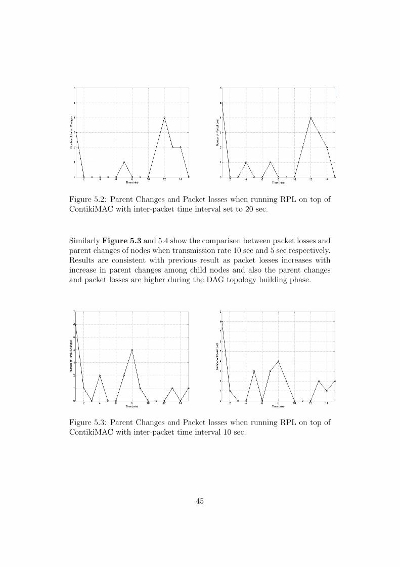
Figure 5.2: Parent Changes and Packet losses when running RPL on top ofContikiMAC with inter-packet time interval set to 20 sec.

Similarly Figure 5.3 and 5.4 show the comparison between packet losses andparent changes of nodes when transmission rate 10 sec and 5 sec respectively.Results are consistent with previous result as packet losses increases withincrease in parent changes among child nodes and also the parent changesand packet losses are higher during the DAG topology building phase.

Figure 5.3: Parent Changes and Packet losses when running RPL on top ofContikiMAC with inter-packet time interval 10 sec.

45

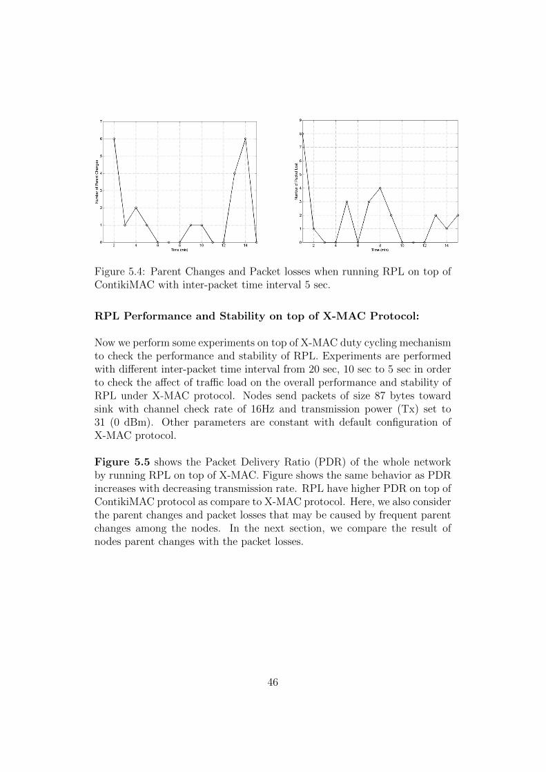
Figure 5.4: Parent Changes and Packet losses when running RPL on top ofContikiMAC with inter-packet time interval 5 sec.

RPL Performance and Stability on top of X-MAC Protocol:

Now we perform some experiments on top of X-MAC duty cycling mechanismto check the performance and stability of RPL. Experiments are performedwith different inter-packet time interval from 20 sec, 10 sec to 5 sec in orderto check the affect of traffic load on the overall performance and stability ofRPL under X-MAC protocol. Nodes send packets of size 87 bytes towardsink with channel check rate of 16Hz and transmission power (Tx) set to31 (0 dBm). Other parameters are constant with default configuration ofX-MAC protocol.

Figure 5.5 shows the Packet Delivery Ratio (PDR) of the whole networkby running RPL on top of X-MAC. Figure shows the same behavior as PDRincreases with decreasing transmission rate. RPL have higher PDR on top ofContikiMAC protocol as compare to X-MAC protocol. Here, we also considerthe parent changes and packet losses that may be caused by frequent parentchanges among the nodes. In the next section, we compare the result ofnodes parent changes with the packet losses.

46

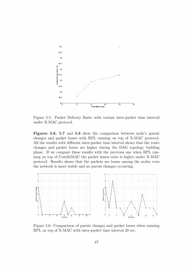
Figure 5.5: Packet Delivery Ratio with variant inter-packet time intervalunder X-MAC protocol.

Figures 5.6, 5.7 and 5.8 show the comparison between node’s parentchanges and packet losses with RPL running on top of X-MAC protocol.All the results with different inter-packet time interval shows that the routechanges and packet losses are higher during the DAG topology buildingphase. If we compare these results with the previous one when RPL run-ning on top of ContikiMAC the packet losses ratio is higher under X-MACprotocol. Results shows that the packets are losses among the nodes eventhe network is more stable and no parent changes occurring.

Figure 5.6: Comparision of parent changes and packet losses when runningRPL on top of X-MAC with inter-packet time interval 20 sec.

47

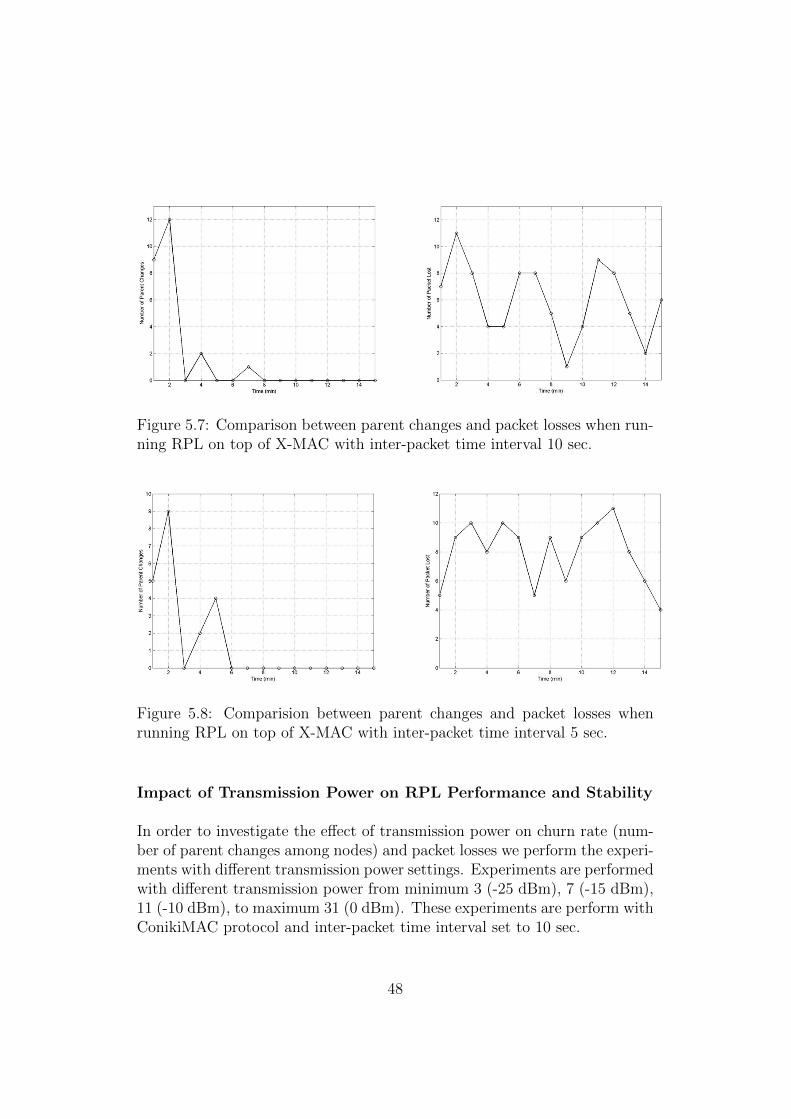
Figure 5.7: Comparison between parent changes and packet losses when run-ning RPL on top of X-MAC with inter-packet time interval 10 sec.

Figure 5.8: Comparision between parent changes and packet losses whenrunning RPL on top of X-MAC with inter-packet time interval 5 sec.

Impact of Transmission Power on RPL Performance and Stability

In order to investigate the effect of transmission power on churn rate (num-ber of parent changes among nodes) and packet losses we perform the experi-ments with different transmission power settings. Experiments are performedwith different transmission power from minimum 3 (-25 dBm), 7 (-15 dBm),11 (-10 dBm), to maximum 31 (0 dBm). These experiments are perform withConikiMAC protocol and inter-packet time interval set to 10 sec.

48

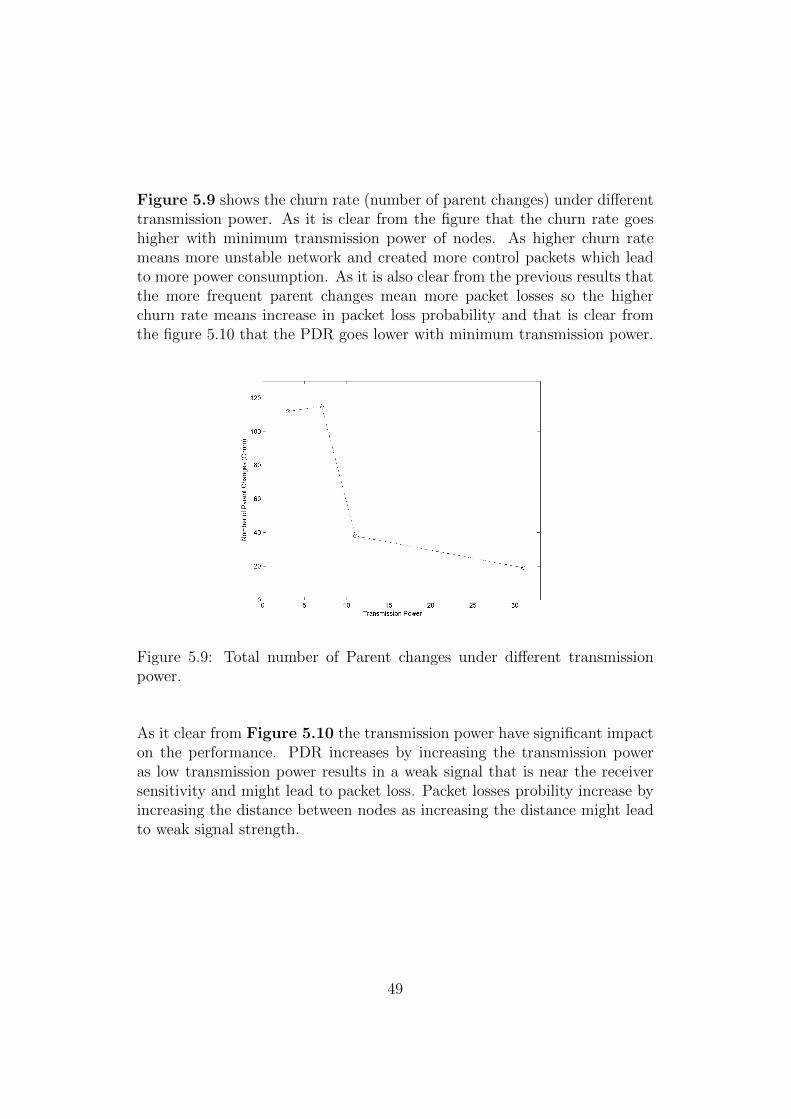
Figure 5.9 shows the churn rate (number of parent changes) under differenttransmission power. As it is clear from the figure that the churn rate goeshigher with minimum transmission power of nodes. As higher churn ratemeans more unstable network and created more control packets which leadto more power consumption. As it is also clear from the previous results thatthe more frequent parent changes mean more packet losses so the higherchurn rate means increase in packet loss probability and that is clear fromthe figure 5.10 that the PDR goes lower with minimum transmission power.

Figure 5.9: Total number of Parent changes under different transmissionpower.

As it clear from Figure 5.10 the transmission power have significant impacton the performance. PDR increases by increasing the transmission poweras low transmission power results in a weak signal that is near the receiversensitivity and might lead to packet loss. Packet losses probility increase byincreasing the distance between nodes as increasing the distance might leadto weak signal strength.

49

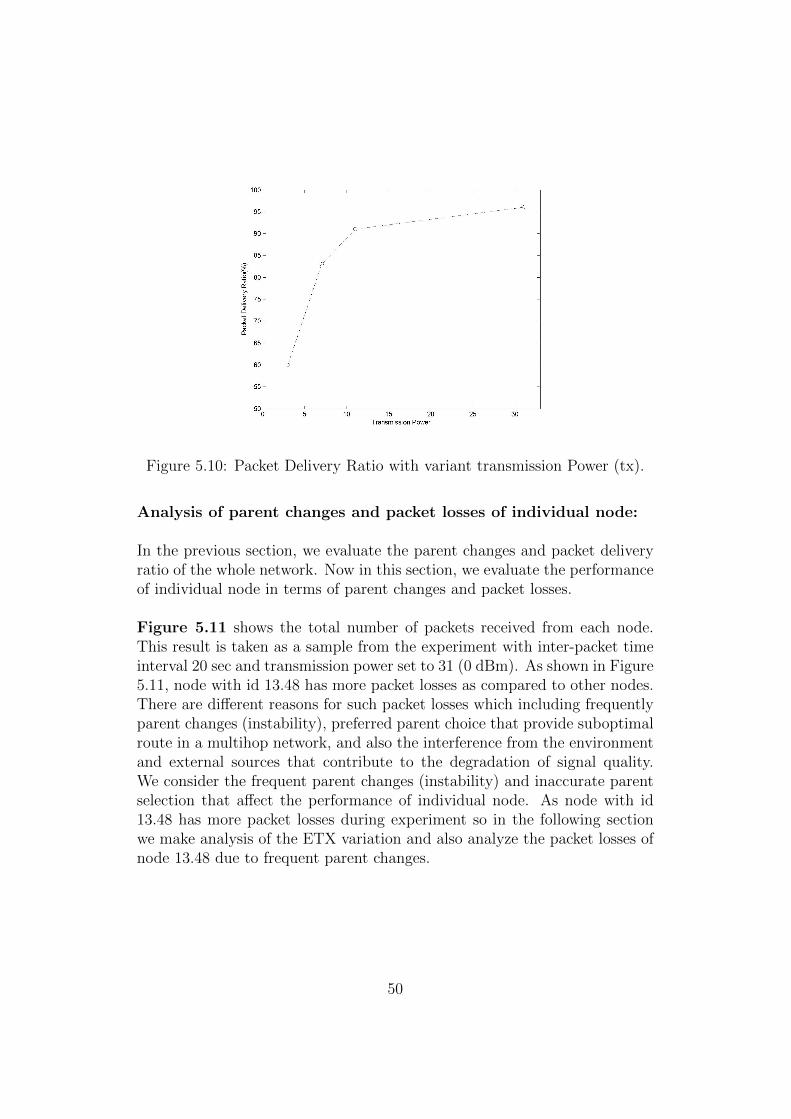
Figure 5.10: Packet Delivery Ratio with variant transmission Power (tx).

Analysis of parent changes and packet losses of individual node:

In the previous section, we evaluate the parent changes and packet deliveryratio of the whole network. Now in this section, we evaluate the performanceof individual node in terms of parent changes and packet losses.

Figure 5.11 shows the total number of packets received from each node.This result is taken as a sample from the experiment with inter-packet timeinterval 20 sec and transmission power set to 31 (0 dBm). As shown in Figure5.11, node with id 13.48 has more packet losses as compared to other nodes.There are different reasons for such packet losses which including frequentlyparent changes (instability), preferred parent choice that provide suboptimalroute in a multihop network, and also the interference from the environmentand external sources that contribute to the degradation of signal quality.We consider the frequent parent changes (instability) and inaccurate parentselection that affect the performance of individual node. As node with id13.48 has more packet losses during experiment so in the following sectionwe make analysis of the ETX variation and also analyze the packet losses ofnode 13.48 due to frequent parent changes.

50

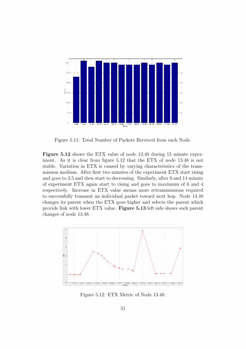
Figure 5.11: Total Number of Packets Received from each Node.

Figure 5.12 shows the ETX value of node 13.48 during 15 minute exper-iment. As it is clear from figure 5.12 that the ETX of node 13.48 is notstable. Variation in ETX is caused by varying characteristics of the trans-mission medium. After first two minutes of the experiment ETX start risingand goes to 3.5 and then start to decreasing. Similarly, after 9 and 14 minuteof experiment ETX again start to rising and goes to maximum of 6 and 4respectively. Increase in ETX value means more retransmissions requiredto successfully transmit an individual packet toward next hop. Node 13.48changes its parent when the ETX goes higher and selects the parent whichprovide link with lower ETX value. Figure 5.13 left side shows such parentchanges of node 13.48.

Figure 5.12: ETX Metric of Node 13.48.

51

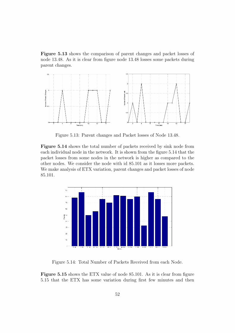
Figure 5.13 shows the comparison of parent changes and packet losses ofnode 13.48. As it is clear from figure node 13.48 losses some packets duringparent changes.

Figure 5.13: Parent changes and Packet losses of Node 13.48.

Figure 5.14 shows the total number of packets received by sink node fromeach individual node in the network. It is shown from the figure 5.14 that thepacket losses from some nodes in the network is higher as compared to theother nodes. We consider the node with id 85.101 as it losses more packets.We make analysis of ETX variation, parent changes and packet losses of node85.101.

Figure 5.14: Total Number of Packets Received from each Node.

Figure 5.15 shows the ETX value of node 85.101. As it is clear from figure5.15 that the ETX has some variation during first few minutes and then

52

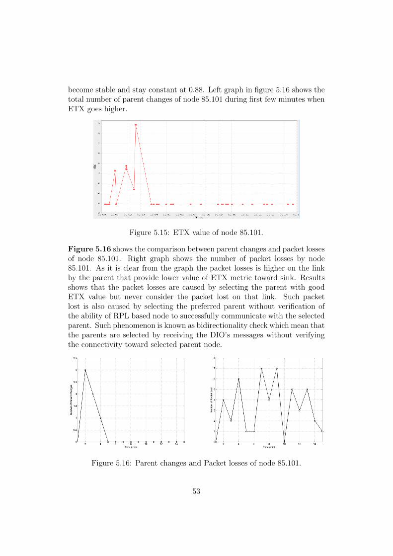
become stable and stay constant at 0.88. Left graph in figure 5.16 shows thetotal number of parent changes of node 85.101 during first few minutes whenETX goes higher.

Figure 5.15: ETX value of node 85.101.

Figure 5.16 shows the comparison between parent changes and packet lossesof node 85.101. Right graph shows the number of packet losses by node85.101. As it is clear from the graph the packet losses is higher on the linkby the parent that provide lower value of ETX metric toward sink. Resultsshows that the packet losses are caused by selecting the parent with goodETX value but never consider the packet lost on that link. Such packetlost is also caused by selecting the preferred parent without verification ofthe ability of RPL based node to successfully communicate with the selectedparent. Such phenomenon is known as bidirectionality check which mean thatthe parents are selected by receiving the DIO’s messages without verifyingthe connectivity toward selected parent node.

Figure 5.16: Parent changes and Packet losses of node 85.101.

53

Chapter 6

Conclusion and Future Work

This thesis presented a performance and network stability evaluation of theIETF RPL routing protocol using an implementation in Contiki 2.5 with twodifferent Radio duty cycling mechanisms ContikiMAC and X-MAC. Experi-ments were performed with differen inter-packet time intervals and transmis-sion power in order to check which condition and configuration have signifi-cant effect on network stability and overall performance. Experiments wereperformed on a real testbed of Tmote sky platforms in a realistic indoorenvironment.

Results showed that the transmission rates affect the overall network PDR inboth cases with ContikiMAC and X-MAC protocol. There is some variationin churn rate under different transmission rates. Compared with the X-MACprotocol, RPL have good performance on top of ContikiMAC and provideshigher packet delivery ratio. Experiments are also performed with differenttransmission power and results showed that the churn rate goes higher underlow transmission power and can cause to increase in packet losses as lowtransmission power might lead to a weak signal. Results also showed that atsome points the packet losses are caused by selecting the parent that providea link with good ETX value but never consider the number of packet losseson that link. Another reason that can cause the packet losses is by selectingthe parent without verifying the bidirectionality of link.

RPL performance is now evaluated in an indoor environment with a smallnumber of nodes and it is very important to evaluate the RPL performancein a large outdoor environment with more than 100 nodes. This thesis fo-cuses only on two MAC layer duty cycling protocols, the next step is toconsider other available radio duty cycling protocols and study the delaythat is caused by parent changes. RPL implementation is depends upon the

54

objective function with ETX metric in order to select the path that sometime provides suboptimal paths. Further research and work is needed to addmore metrics in the implementation of RPL that fulfill the requirements offuture WSN applications.

55

Bibliography

[1] W. Dargie, and C. Poellabauer, Fundamentals of Wireless Sensor Net-works, 2010.

[2] J. Ko, C. Lu, M. Srivastava, J. Stankovic, A. Terzis,and M. Welsh, Wireless Sensor Networks for Healthcare.http://www.cse.wustl.edu/ lu/papers/pieee10.pdf

[3] Verena Weber, Smart Sensor Networks: Technologiesand Applications for Green Growth, December 2009.http://www.oecd.org/dataoecd/39/62/44379113.pdf

[4] P. Park, C. Fischione, A. Bonivento, KH. Johansson, A. Sangiovanni-Vincent, Breath: An adaptive protocol for insutrial control applicationsusing wireless sensor networks, Mobile Computing, IEEE Transactionson 10(6), 821-838.

[5] C. Fischione, P. Park, P Di Marco, KH. Johansson, Design principlesof wireless sensor networks protocols for control applications, WirelessNetworking Based Control, 203.

[6] Culler, D. Estrin, and M. Srivastava, Overview of Sensor Networks,California USA.

[7] Yazeed Al-Obaisat, and R. Braun, On Wireless Sensor Networks: Ar-chitectures, Protocols, Applications and Management.

[8] C. Fischione, Fast-Lipschitz Optimization with Wireless Sensor Net-works Applications, IEEE Transactions on Automatic Control, Vol. 56,No. 10, pp. 2319-2331, october 2011.

[9] Ian F. Akyildiz, and Mehmet Can Vuran, Wireless Sensor Networks.

[10] Sinem Coleri Ergan: ZigBee/802.15.4 Summary, September 10, 2004.

56

[11] P Di Marco, P. Park, C. Fischione, KH.Johansson, TREnD: a timely,reliable, energy-efficient and dynamic wsn protocol for control appli-cations, Communications (ICC), 2010 IEEE International Conference,1-6.

[12] R. Draves, J. Padhye, and B. Zill, Routing in multi-radio, multi-hopwireless mesh networks, in Proceedings of the 10th Annual InternationalConference on Mobile Computing and Networking, pp. 114128, 2004.

[13] F. Silva, J. Heidemann, R. Govindan, and D. Estrin, Directed Diffusion,February 10, 2004.

[14] R. Patel, S. Pariyani, and V. Ukani, Energy and Throughput Analysis ofHierarchical Routing Protocol (LEACH) for Wireless Sensor Network,International Journal of Computer Applications, Volume 20-No.4, April2011.

[15] B. Karp, and HT. Kung, GPSR: Greedy Perime-ter Stateless Routing for Wireless Networks,http://www.eecs.harvard.edu/htk/publication/2000-mobi-karp-kung.pdf

[16] T. He, J. Stankovic, C. Lu, and T. Abdelzaher, SPEED:A Real-Time Routing Protocol for Sensor Networks.http://www.cs.virginia.edu/techrep/CS-2002-09.pdf

[17] The ROLL Design Team. Industrial Routing Require-ments in Low-Power and Lossy Networks, RFC 5673.https://datatracker.ietf.org/doc/draft-ietf-roll-indus-routingreqs

[18] The ROLL Design Team. Home Automation Routing Requirements inLow-Power and Lossy Networks, RFC 5826.

[19] The ROLL Design Team. Building Automation Routing Requirementsin Low-Power and Lossy Networks, RFC 5867.

[20] The ROLL Design Team. Charter of the ROLL work-ing group. IETF, Description of Working Group,http://datatracker.ietf.org/wg/roll/charter/, accessed June, 2010.

[21] ROLL Design Team. RPL: IPv6 Routing Protocol for Low Power andLossy Networks, 2010.

[22] RPL. http://openwsn.berkeley.edu/wiki/OpenRpl.

57

[23] A. Dunkels, B. Gronvall, and T. Voigt. Contiki - a lightweight and flex-ible operating system for tiny networked sensors. In Workshop on Em-bedded Networked Sensors, Tampa, Florida, USA, November 2004.

[24] A. Dunkels, F. Osterlind, Contiki Programming Course.

[25] A. Dunkels. Full TCP/IP for 8-bit architectures. In Proceedings of TheFirst International Conference on Mobile Systems, Applications, andServices (MOBISYS 03), May 2003.

[26] JG. Ko, J. Eriksson, N. Tsiftes, S. Dawson-Haggerty, A. Terzis, A.Dunkels, D. Culler, ContikiRPL and TinyRPL: Happy Together, IPSN11, April 12-14, 2011, Chicago, Illinois.

[27] Y. Chen, JP. Chanet, KM. Hou, RPL Routing Protocol a Case Study:Precision Agriculture, China-France Workshop, February 16-17 2012.

[28] A. Dunkels, The ContikiMAC Radio Duty Cycling Protocol, SICSReport-ISSN 1100-3154, December 2011.

58