performance analysis of gps augmentation using … planets space, 56, 25–37, 2004 performance...
TRANSCRIPT

Earth Planets Space, 56, 25–37, 2004
Performance analysis of GPS augmentation using JapaneseQuasi-Zenith Satellite System
Falin Wu1, Nobuaki Kubo1, and Akio Yasuda1
1Tokyo University of Marine Science and Technology, 2-1-6 Etchujima, Koto-ku, Tokyo 135-8533, Japan
(Received October 3, 2003; Revised January 7, 2004; Accepted January 7, 2004)
The current GPS satellite constellation provides limited availability and reliability for a country like Japan wheremountainous terrain and urban canyons do not allow a clear skyline to the horizon. At present, the Japanese Quasi-Zenith Satellite System (QZSS) is under investigation through a government-private sector cooperation. QZSS isconsidered a multi-mission satellite system, as it is able to provide communication, broadcasting and positioningservices for mobile users in a specified region with high elevation angle. The performance of a Global NavigationSatellite System (GNSS) can be quantified by availability, accuracy, reliability and integrity. This paper focuses onavailability, accuracy and reliability of GPS with and without augmentation using QZSS. The availability, accuracyand reliability of GPS only and augmented GPS using QZSS in the Asia-Pacific and Australian area is studiedby software simulation. The simulation results are described by the number of visible satellites as a measure ofavailability, geometric dilution of precision as a measure of accuracy and minimal detectable bias, and bias-to-noise rate as a measure of reliability, with spatial and temporal variations. It is shown that QZSS does not onlyimprove the availability and accuracy of GPS positioning, but also enhances the reliability of GPS positioning inJapan and its neighboring area.
1. IntroductionCurrently, Japan leads the world in various applications
of GPS equipment and services for civil use. About fivemillion GPS-equipped cellular phones are in use, and ap-proximately two million GPS-equipped car navigation unitsare sold annually in Japan with a cumulative total of aboutten million units sold from 1993 to 2002 (Petrovski et al.,2003). The spread of civil use of the GPS service in such ar-eas as car navigation, aviation, maritime, mapping, land sur-veying, telecommunications and so forth, calls for reliabilityand availability of the positioning service, which at presenthas some limitations due to the limited satellite visibility typ-ical in Japan because of its urban canyons and mountainousregions. A GEO-stationary satellite system couldn’t meetthese requirements because it has an approximate 45◦ ele-vation angle limitation in mid latitude regions. However, theplanned Japanese Quasi-Zenith Satellite System (QZSS) willaugment GPS to meet these requirements.QZSS is a constellation consisting of several Highly El-
liptic Orbit (HEO) satellites orbiting in different high incli-nation planes with a GEO-synchronous orbital period. Eachsatellite is placed on orbit so as to pass over the same groundtrack at a constant interval. Eccentricity and inclination areselected so that users are able to receive the signal from atleast one of the satellites near the zenith direction (i.e. withhigh elevation angle) at any time. This is the origin of thename Quasi-Zenith Satellite System. Satellite systems likeQZSS that utilize a high inclination orbit are indispensable
Copy right c© The Society of Geomagnetism and Earth, Planetary and Space Sciences(SGEPSS); The Seismological Society of Japan; The Volcanological Society of Japan;The Geodetic Society of Japan; The Japanese Society for Planetary Sciences.
for high latitude regions. The Soviet Union (now Russia) hasused the Molniya orbit for satellite communications since1965. For mid latitude regions, although GEO satellite sys-tems have been utilized in the past, some systems have, how-ever, just been implemented for mobile users. Sirius satelliteradio has started to provide their Digital Audio Broadcasting(DAB) services for mobile users in North America via threeHEO satellites. In Europe, Global Radio is also planningto begin a similar DAB service in a couple of years using asimilar HEO satellite system (Kogure and Kawano, 2003).In this paper we focus on the performance of GPS aug-
mentation using the Japanese QZSS. The constellation andsignal structure of QZSS will be briefly reviewed in Sec-tion 2. The three single baseline models and stochastic modelof GPS augmentation using QZSS will be analyzed in Sec-tion 3. The measures for performance analysis will be pre-sented in Section 4. The performance of the GPS augmen-tation using QZSS will be shown in terms of the Numberof Visible Satellites (NVS), Geometric Dilution Of Preci-sion (GDOP), Minimal Detectable Bias (MDB) and Bias-to-Noise Rate (BNR) with spatial and temporal variations inSection 5.
2. Japanese Quasi-Zenith Satellite SystemQZSS is a new concept developed by the private sector,
with the government sector assuming responsibility for theassociated technology development, and especially the por-tion of the project concerned with the positioning service.This effort has taken place in the context of Japan-U.S. co-operation in GPS, formalized by the GPS Joint Statementsigned on November 22, 1998. The 1998 policy statementestablished a cooperative mechanism that provided for an-
25

26 F. WU et al.: PERFORMANCE ANALYSIS OF GPS AUGMENTATION USING JAPANESE QZSS
Table 1. Parameters of the three QZSS satellite constellation options.
QZSS option Ground track Satellite number Eccentricity Inclination Semi-major axis
1 Asymmetrical 8-shape 3 0.099 45.0◦ 42,164 km
2 Egg-shape 3 0.360 52.6◦ 42,164 km
3 Symmetrical 8-shape 3 0.000 45.0◦ 42,164 km
60 90 120 150 180 210−90
−60
−30
0
30
60
90
Longitude [deg]
Latit
ude
[deg
]
(a) Option 1
60 90 120 150 180 210−90
−60
−30
0
30
60
90
Longitude [deg]
Latit
ude
[deg
]
(b) Option 2
60 90 120 150 180 210−90
−60
−30
0
30
60
90
Longitude [deg]
Latit
ude
[deg
]
(c) Option 3
Fig. 1. Ground tracks of the three QZSS satellite constellation options.
nual plenary meetings and working groups. Japan’s statedpolicy objective is “to secure and enhance user interest”, andthe QZSS initiative is a logical outcome of this policy (Petro-vski et al., 2003).2.1 Satellite constellationFive types of constellations that are being considered for
QZSS were registered with the International Telecommuni-cations Union in November 2002 (Petrovski et al., 2003).It is yet to be decided which satellite constellation will beselected for the QZSS, because the investigations are stillunder way. Table 1 summarizes the main characteristics ofthe three most favored satellite constellations that will be in-vestigated in this study. Each satellite constellation optionis composed of three satellites on orbit and one spare satel-lite on the ground. The semi-major axis of all three satel-lite constellations is 42,164 km. Different eccentricity andinclination are selected for the three satellite constellations.Figure 1 shows the ground tracks of the three satellite con-stellations. The eccentricities of the three satellite constella-tions are approximately 0.099, 0.360 and 0.000. Inclinationsof the three satellite constellations are approximately 45.0◦,52.6◦ and 45.0◦ (Kogure and Kawano, 2003; Kon, 2003).
2.1.1 QZSS option 1 With eccentricity 0.099 and in-clination 45.0◦, the ground track of the satellite constellationscribes an asymmetrical figure 8-shape. This satellite con-stellation option focuses on the benefit for mobile commu-nication users with tracking antenna and feeder link stationsin Japan. One advantage of this satellite constellation is thatvarious services, such as communication, broadcasting andpositioning, will be available equally to users in Japan andneighboring countries.
2.1.2 QZSS option 2 With eccentricity 0.360 and in-clination 52.6◦, the ground track of the satellite constellationscribes an egg-shape figure. The advantage of this satellite
constellation option is that broadcasting related services willbe provided a little more effectively for users in Japan andits neighboring countries than in the case of the two othersatellite constellation options.
2.1.3 QZSS option 3 With eccentricity 0.000 and in-clination 45.0◦, the ground track of the satellite constellationscribes a symmetrical figure 8-shape centred on the equator,and users in both hemispheres can receive services equallyeffectively. But this satellite constellation option has to ma-neuver the satellite frequently to avoid collisions as a satellitepasses through the highly populated geostationary satellitebelt. In addition this satellite constellation would provideless favorable visibility over the northern hemisphere com-pared with the two other satellite constellation options.Figure 2 shows the temporal variations of elevation for the
three QZSS satellite constellations at Tokyo. It is shown thata user can track at least one QZSS satellite with 70◦ maskelevation, and two QZSS satellites with 30◦ mask elevationfor each of the three QZSS satellite constellation.Further information about the QZSS satellite constella-
tions can be found in Murotani et al. (2003), Kawano (1999),Takahashi et al. (1999), Kimura and Tanaka (2000), Kawano,(2001), and Yamamoto and Kimura (2003).2.2 Signal structureAt the GPS-QZSS Technical Working Group meeting in
early December 2002, Japanese and U.S. government repre-sentatives discussed the creation of QZSS. The representa-tives from the two nations deliberated the technical require-ments for the QZSS signal structure, codes and power. Todate, the positioning service of QZSS is considered to be anadvanced space augmentation system for GPS. QZSS willuse the same signal structure as GPS, and employ pseudoran-dom noise (PRN) code which used by the GPS constellationand WAAS. Other types of signal modulation are also un-

F. WU et al.: PERFORMANCE ANALYSIS OF GPS AUGMENTATION USING JAPANESE QZSS 27
4.4 4.5 4.6 4.7 4.8 4.9 5 5.1
x 105
0
20
40
60
80
Time [sec]
Ele
vatio
n [d
eg]
(a) QZSS option 1
4.4 4.5 4.6 4.7 4.8 4.9 5 5.1
x 105
0
20
40
60
80
Time [sec]
Ele
vatio
n [d
eg]
(b) QZSS option 2
4.4 4.5 4.6 4.7 4.8 4.9 5 5.1
x 105
0
20
40
60
80
Time [sec]
Ele
vatio
n [d
eg]
(c) QZSS option 3
Fig. 2. Elevation temporal variations of the three QZSS satellite constellations at Tokyo.
Table 2. Possible signals of GPS and QZSS, with corresponding frequen-cies, wavelengths and typical code measurement accuracy.
Signal Frequency Wavelength σcode
[MHz] [m] [m]
L1 1575.42 0.1903 0.30
L2 1227.60 0.2442 0.30
L5 1176.45 0.2548 0.10
der consideration. Currently, the governmental institutionsinvolved continue to work towards a definition of the sig-nal structure. At the time of writing of this paper the latestmeeting had been held in May, 2003 (Petrovski et al., 2003;Kogure and Kawano, 2003).Table 2 gives an overview of possible GPS and QZSS sig-
nals, with corresponding frequencies, wavelengths and typi-cal code measurement accuracy (Shaw et al., 2002; Teunis-sen et al., 2002; Verhagen, 2002b) that are used in this study.
3. GPS Augmentation Using QZSSThe measured ranges of GPS and QZSS, by pseudorange
and carrier phase respectively, are related to the unknownparameters via the following generic measurement equations(Tiberius et al., 2002),
Psr,i = ρs
r + dr,i − ds,i + f 2L1f 2i
I sr + T s
r + esr,i (1)
�sr,i = ρs
r + δr,i − δs,i − f 2L1f 2i
I sr + T s
r
+λi N sr,i + εs
r,i (2)
where � and P are the carrier phase and pseudorange, re-spectively. ρ is the geometric range from satellite s to re-ceiver r ; i is the L-band frequency signals of GPS and QZSS,i = L1, L2 and L5. f is the frequency of the signal. I is theionospheric delay on L1 frequency and T is the troposphericdelay. d and δ are the clock error for code and carrier phaseobservations, respectively. λ and N are the wavelength andcycle ambiguity number of signal i carrier phase. ε and erepresent the effect of receiver noise on the carrier phase andthe pseudorange, respectively.In this study, the three single baseline models that will
be considered are: geometry-free (GF) model, roving-receiver geometry-based (RR) model and the stationary-receiver geometry-based (SR) model (Teunissen, 1997; Te-unissen, 1998; Teunissen and Jong, 1998; de Jong, 2000;Verhagen, 2002b).3.1 Three single baseline modelsFrom Eq. (1) and (2), the observations, with or without
parameterization in terms of the baseline components, arecollected by type, the code and phase observations on allfrequencies. Then the three single baseline models for kepochs of data can all be written in a generic form (Verhagen,2002b),
y = [Ik ⊗ M ek ⊗ N
] [�
a
]+ n (3)
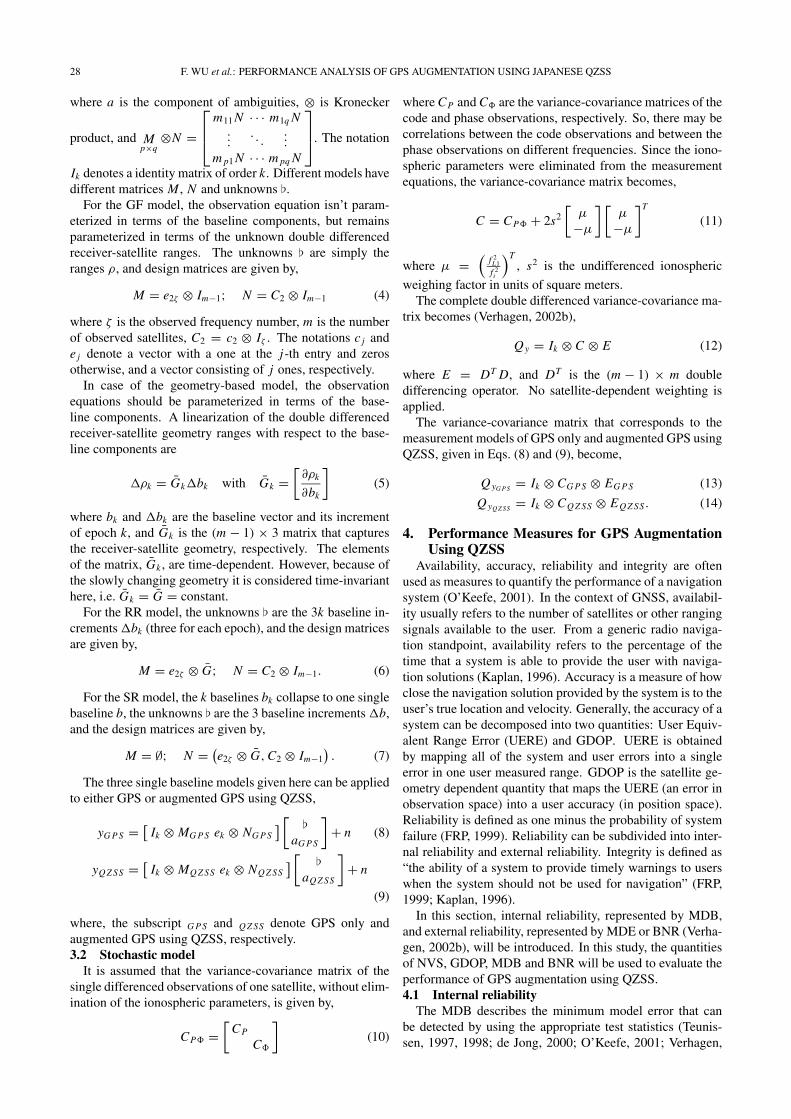
28 F. WU et al.: PERFORMANCE ANALYSIS OF GPS AUGMENTATION USING JAPANESE QZSS
where a is the component of ambiguities, ⊗ is Kronecker
product, and Mp×q
⊗N =
⎡⎢⎣
m11N · · · m1q N...
. . ....
m p1N · · · m pq N
⎤⎥⎦. The notation
Ik denotes a identity matrix of order k. Different models havedifferent matrices M , N and unknowns �.For the GF model, the observation equation isn’t param-
eterized in terms of the baseline components, but remainsparameterized in terms of the unknown double differencedreceiver-satellite ranges. The unknowns � are simply theranges ρ, and design matrices are given by,
M = e2ζ ⊗ Im−1; N = C2 ⊗ Im−1 (4)
where ζ is the observed frequency number, m is the numberof observed satellites, C2 = c2 ⊗ Iζ . The notations c j ande j denote a vector with a one at the j-th entry and zerosotherwise, and a vector consisting of j ones, respectively.In case of the geometry-based model, the observation
equations should be parameterized in terms of the base-line components. A linearization of the double differencedreceiver-satellite geometry ranges with respect to the base-line components are
�ρk = Gk�bk with Gk =[
∂ρk
∂bk
](5)
where bk and �bk are the baseline vector and its incrementof epoch k, and Gk is the (m − 1) × 3 matrix that capturesthe receiver-satellite geometry, respectively. The elementsof the matrix, Gk , are time-dependent. However, because ofthe slowly changing geometry it is considered time-invarianthere, i.e. Gk = G = constant.For the RR model, the unknowns � are the 3k baseline in-
crements�bk (three for each epoch), and the design matricesare given by,
M = e2ζ ⊗ G; N = C2 ⊗ Im−1. (6)
For the SR model, the k baselines bk collapse to one singlebaseline b, the unknowns � are the 3 baseline increments �b,and the design matrices are given by,
M = ∅; N = (e2ζ ⊗ G, C2 ⊗ Im−1
). (7)
The three single baseline models given here can be appliedto either GPS or augmented GPS using QZSS,
yG P S = [Ik ⊗ MG P S ek ⊗ NG P S
] [�
aG P S
]+ n (8)
yQ Z SS = [Ik ⊗ MQ Z SS ek ⊗ NQ Z SS
] [�
aQ Z SS
]+ n
(9)
where, the subscript G P S and Q Z SS denote GPS only andaugmented GPS using QZSS, respectively.3.2 Stochastic modelIt is assumed that the variance-covariance matrix of the
single differenced observations of one satellite, without elim-ination of the ionospheric parameters, is given by,
CP� =[
CP
C�
](10)
where CP and C� are the variance-covariance matrices of thecode and phase observations, respectively. So, there may becorrelations between the code observations and between thephase observations on different frequencies. Since the iono-spheric parameters were eliminated from the measurementequations, the variance-covariance matrix becomes,
C = CP� + 2s2[
μ
−μ
] [μ
−μ
]T
(11)
where μ =(
f 2L1f 2i
)T, s2 is the undifferenced ionospheric
weighing factor in units of square meters.The complete double differenced variance-covariance ma-
trix becomes (Verhagen, 2002b),
Qy = Ik ⊗ C ⊗ E (12)
where E = DT D, and DT is the (m − 1) × m doubledifferencing operator. No satellite-dependent weighting isapplied.The variance-covariance matrix that corresponds to the
measurement models of GPS only and augmented GPS usingQZSS, given in Eqs. (8) and (9), become,
QyG P S = Ik ⊗ CG P S ⊗ EG P S (13)
QyQ Z SS = Ik ⊗ CQ Z SS ⊗ EQ Z SS. (14)
4. Performance Measures for GPS AugmentationUsing QZSS
Availability, accuracy, reliability and integrity are oftenused as measures to quantify the performance of a navigationsystem (O’Keefe, 2001). In the context of GNSS, availabil-ity usually refers to the number of satellites or other rangingsignals available to the user. From a generic radio naviga-tion standpoint, availability refers to the percentage of thetime that a system is able to provide the user with naviga-tion solutions (Kaplan, 1996). Accuracy is a measure of howclose the navigation solution provided by the system is to theuser’s true location and velocity. Generally, the accuracy of asystem can be decomposed into two quantities: User Equiv-alent Range Error (UERE) and GDOP. UERE is obtainedby mapping all of the system and user errors into a singleerror in one user measured range. GDOP is the satellite ge-ometry dependent quantity that maps the UERE (an error inobservation space) into a user accuracy (in position space).Reliability is defined as one minus the probability of systemfailure (FRP, 1999). Reliability can be subdivided into inter-nal reliability and external reliability. Integrity is defined as“the ability of a system to provide timely warnings to userswhen the system should not be used for navigation” (FRP,1999; Kaplan, 1996).In this section, internal reliability, represented by MDB,
and external reliability, represented by MDE or BNR (Verha-gen, 2002b), will be introduced. In this study, the quantitiesof NVS, GDOP, MDB and BNR will be used to evaluate theperformance of GPS augmentation using QZSS.4.1 Internal reliabilityThe MDB describes the minimum model error that can
be detected by using the appropriate test statistics (Teunis-sen, 1997, 1998; de Jong, 2000; O’Keefe, 2001; Verhagen,
F. WU et al.: PERFORMANCE ANALYSIS OF GPS AUGMENTATION USING JAPANESE QZSS 29
2002b; Verhagen and Joosten, 2003). The MDB can be com-puted once the type of model error is specified, so that thenull-hypothesis (H0), which assumes that there is no error,can be tested against the alternative hypothesis (Ha), whichassumes the presence of the error. The two hypotheses aredefined as (Teunissen, 1998)
H0 : E {y} = Ax, D {y} = Qy (15)
Ha : E {y} = Ax + c∇, D {y} = Qy (16)
where E {·} and D {·} are the expectation and dispersionoperators, respectively, y is the p-vector observations, Ais the p × q design matrix, x is the q-vector of unknownparameters, c is a known p-vector which specifies the typeof model error, and ∇ is its unknown size, and Qy is thevariance matrix of the observations.The uniformly most powerful test statistic for testing H0
against Ha is given as (Teunissen, 1998)
T =(cT Q−1
y P⊥A y
)2cT Q−1
y P⊥A c
(17)
where P⊥A = Ip −PA, and PA is the orthogonal projector on
the range space of A, PA = A(
AT Q−1y A
)−1AT Q−1
y . Thetest statistic T has the following Chi-squared distributionsunder H0 and Ha
H0 : T ∼ χ2 (1, 0) ; Ha : T ∼ χ2 (1, λ) (18)
where λ is the non-centrality parameter,
λ = ∇2cT Q−1y P⊥
A c. (19)
The non-centrality parameter λ can be computed when ref-erence values are chosen for the level of confidence α0 (theprobability of rejecting H0 when it is true) and the detec-tion power γ0 (the probability of rejecting H0 when Ha istrue). Once the parameter λ0 = λ(α0, γ0) is known, the cor-responding size of the bias, MDB, that can just be detected,follows from Eq. (19) as (Teunissen, 1998)
|∇| =√
λ0
cT Q−1y P⊥
A c(20)
where P⊥A = Ip − A
(AT Q−1
y A)−1
AT Q−1y .
Potential model errors in GNSS applications are outliers inthe code observations, and/or cycle slips in the carrier phaseobservations. The three single baseline models described inSection 3.1 can be used to find expressions for the corre-sponding MDB using Eq. (20.) The design matrix A of thethree single baseline models follows from the results of Sec-tion 3.1 as
A = [Mk Nk
]with Mk = Ik ⊗ M, Nk = ek ⊗ N (21)
where⎧⎨⎩
M = e2ζ ⊗ Im−1, N = C2 ⊗ Im−1 GFM = e2ζ ⊗ G, N = C2 ⊗ Im−1 RRM = ∅, N = (
e2ζ ⊗ G, C2 ⊗ Im−1)SR
. (22)
It is assumed that the error occurs in the observation onfrequency i at epoch l in the double differenced range to
satellite s ∈ (1, · · · , m), so that the vector c in Eq. (20)becomes
c = cl
sl
}⊗ d, with d = ci
ci+ζ
}⊗ ds
code outliercycle slip.
(23)
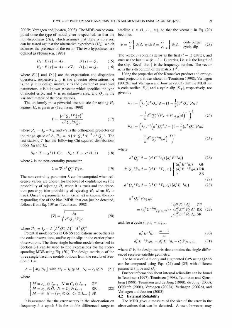
The vector sl contains zeros as the first (l − 1) entries, andones as the last v = (k − l + 1) entries, i.e. v is the length ofthe slip. Recall that ζ is the frequency number. The vectords is the s-th column of the matrix DT .Using the properties of the Kronecker product and orthog-
onal projectors, it was shown in Teunissen (1998), Verhagen(2002b) and Verhagen and Joosten (2003) that the MDB fora code outlier |∇P | and a cycle slip |∇�|, respectively, aregiven by
|∇P | =(
λ0
(dT Q−1
y d − (1 − 1
k
)dT Q−1
y PM d
− 1
kdT Q−1
y
(PN + PP⊥N M
)d)−1
) 12
(24)
|∇�| =(
λ0v−1
(dT Q−1
y d − (1 − v
k
)dT Q−1
y PM d
− v
kdT Q−1
y PN d)−1
) 12
(25)
where
dT Q−1y d = (
cTi C−1ci
) (dT
s E−1ds)
(26)
dT Q−1y PM d = (
cTi C−1Pe2ζ ci
) ⎧⎨⎩
(dTs E−1ds) GF
(dTs E−1PGds) RR
0 SR
(27)
dT Q−1y PN d = (
cTi C−1PC2ci
) (dT
s E−1ds)
(28)
dT Q−1y PP⊥
N M d
= (cTi C−1PP⊥
C2e2ζ ci )
⎧⎨⎩
(dTs E−1ds) GF
(dTs E−1PGds) RR
(dTs E−1PGds) SR
(29)
and, for a cycle slip ci = ci+ζ ,
dTs E−1ds = m − 1
m(30)
dTs E−1PGds = dT
s E−1ds − cTs P[G em ]cs (31)
where G is the design matrix that contains the single differ-enced receiver-satellite geometry.The MDBs of GPS only and augmented GPS using QZSS
can be computed using Eqs. (24) and (25) with differentparameters y, A and Qy .
Further information about internal reliability can be foundin Teunissen (1997), Teunissen (1998), Teunissen and Kleus-berg (1998), Teunissen and de Jong (1998), de Jong (2000),O’Keefe (2001), Verhagen (2002a), Verhagen (2002b), andVerhagen and Joosten (2003).4.2 External ReliabilityThe MDB gives a measure of the size of the error in the
observations that can be detected. A user, however, may
30 F. WU et al.: PERFORMANCE ANALYSIS OF GPS AUGMENTATION USING JAPANESE QZSS
Table 3. Configuration of all scenarios considered in the simulations.
System GPS, GPS+QZSS (three options)
Baseline model Single medium length baseline (20 km) RR model
Code standard deviation σP = 0.300 m
Phase standard deviation σ� = 0.003 m
Ionospheric delay σI = 0.020 m
Tropospheric delay σT = 0.010 m
Mask elevation 30◦
Spatial simulation Date and time Sep. 5, 2003, 12:00
Location Asia-Pacific, Australian area (Lat: 90◦S–90◦N, Lon:60◦–210◦ )
Temporal simulation Date and time Aug. 31, 2003, 00:00–Sep. 6, 2003, 24:00
Location Tokyo (35◦39′59′′N, 139◦47′32′′E)
Output Spatial variation NVS, GDOP, MDB and BNR
Temporal variation NVS, GDOP, MDB and BNR
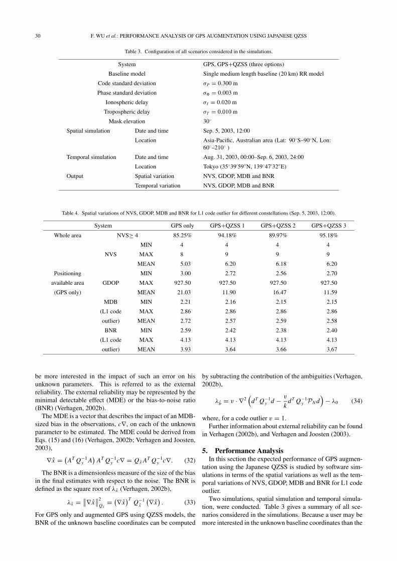
Table 4. Spatial variations of NVS, GDOP, MDB and BNR for L1 code outlier for different constellations (Sep. 5, 2003, 12:00).
System GPS only GPS+QZSS 1 GPS+QZSS 2 GPS+QZSS 3
Whole area NVS≥ 4 85.25% 94.18% 89.97% 95.18%
MIN 4 4 4 4
NVS MAX 8 9 9 9
MEAN 5.03 6.20 6.18 6.20
Positioning MIN 3.00 2.72 2.56 2.70
available area GDOP MAX 927.50 927.50 927.50 927.50
(GPS only) MEAN 21.03 11.90 16.47 11.59
MDB MIN 2.21 2.16 2.15 2.15
(L1 code MAX 2.86 2.86 2.86 2.86
outlier) MEAN 2.72 2.57 2.59 2.58
BNR MIN 2.59 2.42 2.38 2.40
(L1 code MAX 4.13 4.13 4.13 4.13
outlier) MEAN 3.93 3.64 3.66 3.67
be more interested in the impact of such an error on hisunknown parameters. This is referred to as the externalreliability. The external reliability may be represented by theminimal detectable effect (MDE) or the bias-to-noise ratio(BNR) (Verhagen, 2002b).TheMDE is a vector that describes the impact of anMDB-
sized bias in the observations, c∇, on each of the unknownparameter to be estimated. The MDE could be derived fromEqs. (15) and (16) (Verhagen, 2002b; Verhagen and Joosten,2003),
∇ x = (AT Q−1
y A)
AT Q−1y c∇ = Qx AT Q−1
y c∇. (32)
The BNR is a dimensionless measure of the size of the biasin the final estimates with respect to the noise. The BNR isdefined as the square root of λx (Verhagen, 2002b),
λx = ∥∥∇ x∥∥2
Qx= (∇ x
)TQ−1
x
(∇ x). (33)
For GPS only and augmented GPS using QZSS models, theBNR of the unknown baseline coordinates can be computed
by subtracting the contribution of the ambiguities (Verhagen,2002b),
λb = v · ∇2(
dT Q−1y d − v
kdT Q−1
y PN d)
− λ0 (34)
where, for a code outlier v = 1.Further information about external reliability can be found
in Verhagen (2002b), and Verhagen and Joosten (2003).
5. Performance AnalysisIn this section the expected performance of GPS augmen-
tation using the Japanese QZSS is studied by software sim-ulations in terms of the spatial variations as well as the tem-poral variations of NVS, GDOP, MDB and BNR for L1 codeoutlier.Two simulations, spatial simulation and temporal simula-
tion, were conducted. Table 3 gives a summary of all sce-narios considered in the simulations. Because a user may bemore interested in the unknown baseline coordinates than the

F. WU et al.: PERFORMANCE ANALYSIS OF GPS AUGMENTATION USING JAPANESE QZSS 31
Longitude [deg]
Latit
ude
[deg
]
(a) GPS only
60 90 120 150 180 210−90
−60
−30
0
30
60
90
2
3
4
5
6
7
8
9
Longitude [deg]
Latit
ude
[deg
]
(b) GPS and QZSS option 1
60 90 120 150 180 210−90
−60
−30
0
30
60
90
2
3
4
5
6
7
8
9
Longitude [deg]
Latit
ude
[deg
]
(c) GPS and QZSS option 2
60 90 120 150 180 210−90
−60
−30
0
30
60
90
2
3
4
5
6
7
8
9
Longitude [deg]
Latit
ude
[deg
]
(d) GPS and QZSS option 3
60 90 120 150 180 210−90
−60
−30
0
30
60
90
2
3
4
5
6
7
8
9
Fig. 3. Spatial variations of NVS for different constellations.
receiver-satellite ranges and the SR model is a typical formof the RR model, only a single medium length baseline (20km) RR model was considered in the simulations. The ac-curacies of all code and carrier phase observation were set atstandard deviation 0.300 m and 0.003 m, respectively. Iono-spheric slant delays and tropospheric zenith delay and wereincluded as unknown parameters, but the uncertainty in theseparameters’ values had been restricted. Variations in the de-lays were tolerated to a reasonable small extent on a mediumlength baseline (σI = 0.020 m and σT = 0.010 m). It hasbeen shown in Section 2.1 that a user at Tokyo can track atleast two QZSS satellites with 30◦ mask elevation, the visiblesatellites were masked by a 30◦ elevation angle cutoff in thesimulations. To compute the positions of the GPS satellitesand to simulate the positions of the QZSS satellites, a YUMAalmanac was used. The locations of twenty eight GPS satel-lite and the three QZSS options were continuously simulatedfor Sep. 5, 2003, 12:00 for spatial simulation and from Aug.31, 2003, 00:00 to Sep. 6, 2003, 24:00, with a sampling in-terval of 120 seconds, for temporal simulation. The receiver-satellite geometries were simulated in the Asia-Pacific, Aus-tralian and New Zealand area (Latitude: 90◦S–90◦N , Longi-tude: 60◦–210◦), with a sampling grid of 0.4◦×0.4◦, for spa-tial simulation, and in Tokyo (35◦39′59′′N , 139◦47′32′′E)
for temporal simulation. The spatial and temporal simula-tions outputted the spatial variations as well as the temporalvariations of NVS, GDOP, MDB and BNR for L1 code out-lier.
5.1 Spatial variationsBefore considering temporal variations performance of
GPS augmentation using QZSS, the spatial variations per-formances are analyzed.Table 4 summarizes the spatial variations of NVS, GDOP,
MDB and BNR for L1 code outlier in the case of GPSonly and augmented GPS using the three QZSS options atSeptember 5, 2003, 12:00. It is shown that with the augmen-tation by the three QZSS options, the area where positioningis available (NVS ≥ 4) will be extended from 85.25% to94.18%, 89.97% and 95.18%, respectively for each constel-lation. For spatial variations, augmentation using the threeQZSS options can extend the positioning available area, butalso enables some locations that have a very high GDOP,MDB and BNR. To analyze the performance of GPS aug-mentation using the three QZSS options, only the area wherepositioning is available in the case of GPS only is consideredin this subsection.Figure 3 shows the NVS of GPS only and augmented GPS
using the three QZSS options as a function of geographic lo-cation. The maximum NVS of GPS only is 8, but augmentedGPS using the three QZSS options give values 9 for all cases.The average NVS of GPS only is about 5.03, but the valuesof augmented GPS using the three QZSS options are about6.20, 6.18 and 6.20, respectively.Figure 4 shows the spatial variations of GDOP for the GPS
only and augmented GPS using the three QZSS options. Theminimum GDOP of GPS only is about 3.00, but augmentedGPS using the three QZSS options give values 2.72, 2.56 and

32 F. WU et al.: PERFORMANCE ANALYSIS OF GPS AUGMENTATION USING JAPANESE QZSS
Longitude [deg]
Latit
ude
[deg
]
(a) GPS only
60 90 120 150 180 210−90
−60
−30
0
30
60
90
3
4
5
6
7
8
9
10
Longitude [deg]
Latit
ude
[deg
]
(b) GPS and QZSS option 1
60 90 120 150 180 210−90
−60
−30
0
30
60
90
3
4
5
6
7
8
9
10
Longitude [deg]
Latit
ude
[deg
]
(c) GPS and QZSS option 2
60 90 120 150 180 210−90
−60
−30
0
30
60
90
3
4
5
6
7
8
9
10
Longitude [deg]
Latit
ude
[deg
]
(d) GPS and QZSS option 3
60 90 120 150 180 210−90
−60
−30
0
30
60
90
3
4
5
6
7
8
9
10
Fig. 4. Spatial variations of GDOP for different constellations.
Longitude [deg]
Latit
ude
[deg
]
(a) GPS only
60 90 120 150 180 210−90
−60
−30
0
30
60
90
2.2
2.3
2.4
2.5
2.6
2.7
2.8
Longitude [deg]
Latit
ude
[deg
]
(b) GPS and QZSS option 1
60 90 120 150 180 210−90
−60
−30
0
30
60
90
2.2
2.3
2.4
2.5
2.6
2.7
2.8
Longitude [deg]
Latit
ude
[deg
]
(c) GPS and QZSS option 2
60 90 120 150 180 210−90
−60
−30
0
30
60
90
2.2
2.3
2.4
2.5
2.6
2.7
2.8
Longitude [deg]
Latit
ude
[deg
]
(d) GPS and QZSS option 3
60 90 120 150 180 210−90
−60
−30
0
30
60
90
2.2
2.3
2.4
2.5
2.6
2.7
2.8
Fig. 5. Spatial variations of MDB for L1 code outlier for different constellations.
F. WU et al.: PERFORMANCE ANALYSIS OF GPS AUGMENTATION USING JAPANESE QZSS 33
Longitude [deg]
Latit
ude
[deg
]
(a) GPS only
60 90 120 150 180 210−90
−60
−30
0
30
60
90
2.5
3
3.5
4
Longitude [deg]
Latit
ude
[deg
]
(b) GPS and QZSS option 1
60 90 120 150 180 210−90
−60
−30
0
30
60
90
2.5
3
3.5
4
Longitude [deg]
Latit
ude
[deg
]
(c) GPS and QZSS option 2
60 90 120 150 180 210−90
−60
−30
0
30
60
90
2.5
3
3.5
4
Longitude [deg]
Latit
ude
[deg
]
(d) GPS and QZSS option 3
60 90 120 150 180 210−90
−60
−30
0
30
60
90
2.5
3
3.5
4
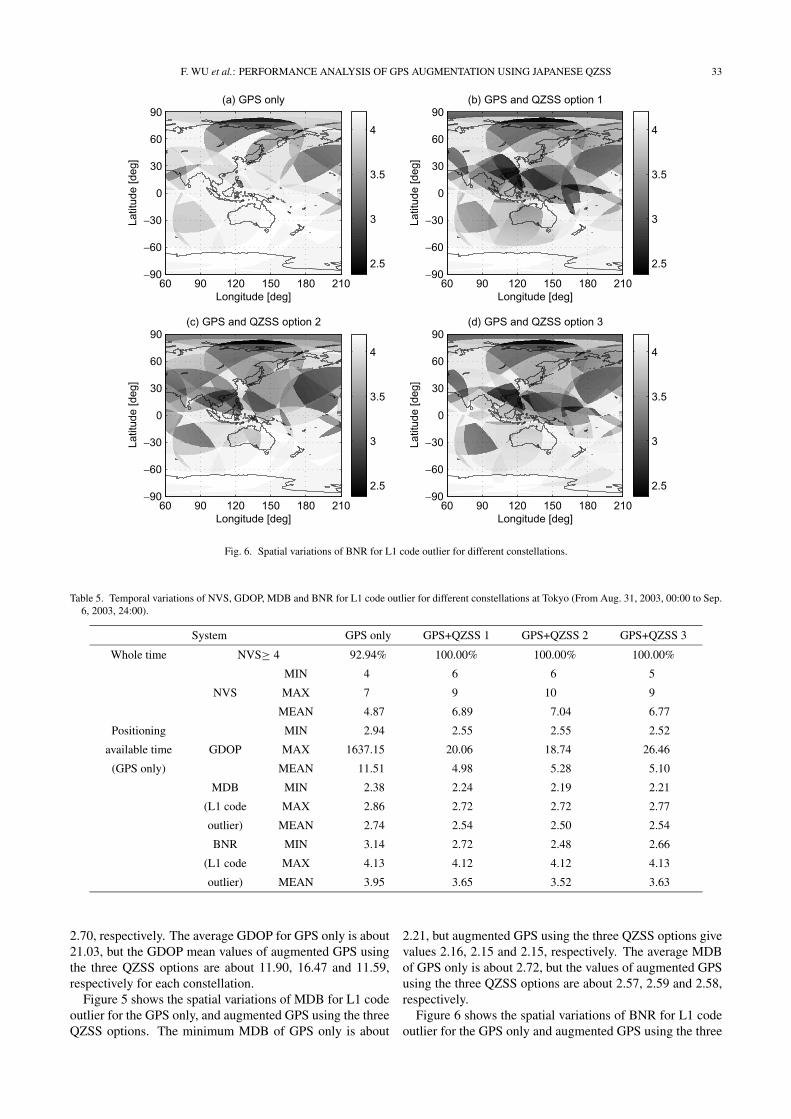
Fig. 6. Spatial variations of BNR for L1 code outlier for different constellations.
Table 5. Temporal variations of NVS, GDOP, MDB and BNR for L1 code outlier for different constellations at Tokyo (From Aug. 31, 2003, 00:00 to Sep.6, 2003, 24:00).
System GPS only GPS+QZSS 1 GPS+QZSS 2 GPS+QZSS 3
Whole time NVS≥ 4 92.94% 100.00% 100.00% 100.00%
MIN 4 6 6 5
NVS MAX 7 9 10 9
MEAN 4.87 6.89 7.04 6.77
Positioning MIN 2.94 2.55 2.55 2.52
available time GDOP MAX 1637.15 20.06 18.74 26.46
(GPS only) MEAN 11.51 4.98 5.28 5.10
MDB MIN 2.38 2.24 2.19 2.21
(L1 code MAX 2.86 2.72 2.72 2.77
outlier) MEAN 2.74 2.54 2.50 2.54
BNR MIN 3.14 2.72 2.48 2.66
(L1 code MAX 4.13 4.12 4.12 4.13
outlier) MEAN 3.95 3.65 3.52 3.63
2.70, respectively. The average GDOP for GPS only is about21.03, but the GDOP mean values of augmented GPS usingthe three QZSS options are about 11.90, 16.47 and 11.59,respectively for each constellation.Figure 5 shows the spatial variations of MDB for L1 code
outlier for the GPS only, and augmented GPS using the threeQZSS options. The minimum MDB of GPS only is about
2.21, but augmented GPS using the three QZSS options givevalues 2.16, 2.15 and 2.15, respectively. The average MDBof GPS only is about 2.72, but the values of augmented GPSusing the three QZSS options are about 2.57, 2.59 and 2.58,respectively.Figure 6 shows the spatial variations of BNR for L1 code
outlier for the GPS only and augmented GPS using the three

34 F. WU et al.: PERFORMANCE ANALYSIS OF GPS AUGMENTATION USING JAPANESE QZSS
0 2 4 6
x 105
2
4
6
8
10
GPS Time [sec]
Num
ber
of V
isib
le S
atel
lites
(a) GPS only
0 2 4 6
x 105
2
4
6
8
10
GPS Time [sec]
Num
ber
of V
isib
le S
atel
lites
(b) GPS and QZSS option 1
0 2 4 6
x 105
2
4
6
8
10
GPS Time [sec]
Num
ber
of V
isib
le S
atel
lites
(c) GPS and QZSS option 2
0 2 4 6
x 105
2
4
6
8
10
GPS Time [sec]
Num
ber
of V
isib
le S
atel
lites
(d) GPS and QZSS option 3
Fig. 7. Temporal variations of NVS for different constellations.
0 1 2 3 4 5 6
x 105
−10
−5
0
GPS Time [sec]
GD
OP
Diff
eren
ce
(a) QZSS option 1
0 1 2 3 4 5 6
x 105
−10
−5
0
GPS Time [sec]
GD
OP
Diff
eren
ce
(b) QZSS option 2
0 1 2 3 4 5 6
x 105
−10
−5
0
GPS Time [sec]
GD
OP
Diff
eren
ce
(c) QZSS option 3
Fig. 8. Temporal variations of GDOP difference between having QZSS augmentation and not having it (three QZSS options).

F. WU et al.: PERFORMANCE ANALYSIS OF GPS AUGMENTATION USING JAPANESE QZSS 35
0 1 2 3 4 5 6
x 105
−0.6
−0.4
−0.2
0
GPS Time [sec]
MD
B D
iffer
ence
(a) QZSS option 1
0 1 2 3 4 5 6
x 105
−0.6
−0.4
−0.2
0
GPS Time [sec]
MD
B D
iffer
ence
(b) QZSS option 2
0 1 2 3 4 5 6
x 105
−0.6
−0.4
−0.2
0
GPS Time [sec]
MD
B D
iffer
ence
(c) QZSS option 3
Fig. 9. Temporal variations of L1 code outlier MDB difference between having QZSS augmentation and not having it (three QZSS options).
QZSS options. The minimum BNR of GPS only is about2.59, but augmented GPS using the three QZSS options givevalues 2.42, 2.38 and 2.40, respectively. The BNR meanvalue for GPS only is about 3.93, but the BNR mean valuesof augmented GPS using the three QZSS options are about3.64, 3.66 and 3.67, respectively for each constellation.It has been shown that any of the three QZSS options
will not only extend the positioning available area, and im-prove the satellite visibility, and offer better GDOP, but alsoenhance the system reliability in Japan and its neighboringarea. From the three QZSS options, QZSS option 3 can pro-vide a little more favorable availability and accuracy than inthe case of the two other QZSS options. But QZSS option 1can provide a little more favorable availability, accuracy andreliability than in the case of QZSS option 2.5.2 Temporal VariationsTable 5 summarizes the temporal variations of NVS,
GDOP, MDB and BNR for L1 code outlier in the case ofGPS only, and augmented GPS for the three QZSS optionsat Tokyo from August 31, 2003, 00:00 to September 6, 2003,24:00. It is shown that with the augmentation by any of thethree QZSS options, the time when positioning is available(NVS ≥ 4) will be improved from 92.94% to 100.00%. Fortemporal variations, augmentation using the three QZSS op-tions can improve the positioning available time, but also en-ables some moments when have a very high GDOP, MDB
and BNR. To analyze the performance of GPS augmentationusing the three QZSS options, only the time when position-ing is available in the case of GPS only is considered in thissubsection.Figure 7 shows the variation of NVS for the GPS only
and augmented GPS using the three QZSS options over aone week period. The maximum NVS of GPS only is 7, butaugmented GPS using the three QZSS options give values9, 10 and 9, respectively. The average NVS of GPS only isabout 4.87, but the values of augmented GPS using the threeQZSS options are about 6.89, 7.04 and 6.77, respectively foreach constellation.The minimum GDOP of GPS only is about 2.94, but aug-
mented GPS using the three QZSS options give vlues 2.55,2.55 and 2.52, respectively. The GDOP mean values of GPSonly and augmented GPS using the three QZSS options are11.51, 4.98, 5.28 and 5.10, respectively. Figure 8 shows theGDOP differences between having QZSS augmentation andnot having it as a function of time.The minimum MDB of GPS only is about 2.38, but the
augmented GPS using the three QZSS options give values2.24, 2.19 and 2.21, respectively. The MDB mean value ofGPS only is about 2.74, but the MDB mean values of aug-mented GPS using the three QZSS options are about 2.54,2.50 and 2.54, respectively. Figure 9 shows the temporalvariations of L1 code outlier MDB difference between hav-

36 F. WU et al.: PERFORMANCE ANALYSIS OF GPS AUGMENTATION USING JAPANESE QZSS
0 1 2 3 4 5 6
x 105
−2
−1.5
−1
−0.5
0
0.5
GPS Time [sec]
BN
R D
iffer
ence
(a) QZSS option 1
0 1 2 3 4 5 6
x 105
−2
−1.5
−1
−0.5
0
0.5
GPS Time [sec]
BN
R D
iffer
ence
(b) QZSS option 2
0 1 2 3 4 5 6
x 105
−2
−1.5
−1
−0.5
0
0.5
GPS Time [sec]
BN
R D
iffer
ence
(c) QZSS option 3
Fig. 10. Temporal variations of L1 code outlier BNR difference between having QZSS augmentation and not having it (three QZSS options).
ing QZSS augmentation and not having it.The minimum BNR of GPS only is about 3.14, but the
augmented GPS using the three QZSS options give values2.72, 2.48 and 2.66, respectively. The BNR mean value ofGPS only is about 3.95, but the BNR mean values of aug-mented GPS using the three QZSS options are 3.65, 3.52and 3.63, respectively. Figure 10 shows the temporal varia-tions of the L1 code outlier BNR difference between havingQZSS augmentation and not having it.The results show that any of the three QZSS options will
not only improve the positioning available time, and improvethe satellite visibility, and offer better GDOP, but also willenhance the system reliability across Japan. From the threeQZSS options, QZSS option 2 can provide a little morefavorable availability and reliability than in case of the twoother QZSS options, but QZSS option 1 can provide a littlemore favorable accuracy than in the case of the two otherQZSS options.
6. ConclusionsThis paper has focussed on the performance of GPS aug-
mentation using the proposed Japanese QZSS. The QZSSsatellite constellation and signal structure have been brieflyintroduced. The three single baseline models and stochas-tic model of GPS augmentation using QZSS have been ana-lyzed. The measures for performance analysis, NVS, GDOP,MDB, MDE and BNR, have been described. The achievable
performance of the GPS augmentation using QZSS are ob-tained using software simulation, and described by the spa-tial and temporal variations of NVS, GDOP, MDB and BNR.Three QZSS satellite constellation options have been inves-tigated. It has been shown that QZSS does not only effec-tively improve the availability and accuracy of GPS position-ing, but also enhances the reliability of GPS positioning inJapan and its neighboring area. From the three QZSS op-tions, QZSS option 1 is the best satellite constellation optionfor Japan, although QZSS option 3 is the best satellite con-stellation option for the whole Asia-Pacific, Australian andNew Zealand area.
Acknowledgments. The authors would like to acknowledgeDr. Tomoyuki Miyano, Tokyo Metropolitan College of Aeronauti-cal Engineering, and Mr. Masayuki Saito, Advanced Space Busi-ness Corporation, Japan, for discussions on QZSS satellite con-stellation. The authors would also like to acknowledge Mr. PeterJoosten and Ms. Sandra Verhagen, Delft University of Technology,for software support.
Referencesde Jong, C. D., Minimal detectable biases of cross-correlated GPS observa-
tions, GPS Solutions, 3(3), 12–18, 2000.FRP, Federal Radionavigation Plan, Final Report DOD-4650.5, United
States Department of Defence and Department of Transportation, Wash-ington, D.C. 20590, USA, 1999.
Kaplan, E. D., Understanding GPS—Principles and Applications, Artech
F. WU et al.: PERFORMANCE ANALYSIS OF GPS AUGMENTATION USING JAPANESE QZSS 37
House, Boston, 1996.Kawano, I., System Study of Next Generation Satellite Positioning System,
SANE 98-144, Institute of Electronics, Information and CommunicationEngineers, 1999 (in Japanese).
Kawano, I., Satellite Positioning System Using Quasi-Zenith and Geosta-tionary Satellites, The transactions of the Institute of Electronics, Infor-mation and Communication Engineers, J84-B:2092–2100, 2001.
Kimura, K. and M. Tanaka, Inclined Geo-synchronous Orbit Constella-tions Suitable to Fixed Satellite Communications, SANE 99-123, Insti-tute of Electronics, Information and Communication Engineers, 2000 (inJapanese).
Kogure, S. and I. Kawano, GPS Augmentation and Complement UsingQuasi-Zenith Satellite System (QZSS), Proceeding of the 21st AIAA In-ternational Communications Satellite Systems, Yokohama, Japan, 2003.
Kon, M., System Overview and Applications of Quasi-Zenith Satellite Sys-tems, Proceeding of the 21st AIAA International Communications Satel-lite Systems, Yokohama, Japan, 2003,
Murotani, M., S. Urasaki, and O. Yamanaka, Quasi-geostationary orbit andapplication in communication, broadcast and positioning, Research onSatellite Communication, 101, 1–77, 2003 (in Japanese).
O’Keefe, K., Availability and Reliability Advantages of GPS/Galileo Inte-gration, Proceeding of the 14th International Technical Meeting of theSatellite Division of the Institute of Navigation (ION GPS-2001), pp.2096–2104, Salt Lake City, UT, USA, 2001.
Petrovski, I. G., M. Ishii, H. Torimoto, H. Kishimoto, T. Furukawa, M. Saito,T. Tanaka, and H.Maeda, QZSS—Japan’s new integrated communicationand positioning service for mobile users, GPS World, 14(6), 24–29, 2003.
Shaw, M., D. A. Turner, and K. Sandhoo, Modernization of the GlobalPositioning System, Proceeding of the Japanese Institute of Navigation,GPS Symposium 2002, pp. 3–12, Tokyo, Japan, 2002.
Takahashi, M., K. Kimura, and M. Tanaka, An Adaptability Study of Quasi-Zenith Satellite Orbits for LandMobile Satellite Communications, SANE99-31, Institute of Electronics, Information and Communication Engi-neers, 1999 (in Japanese).
Teunissen, P. J. G., Internal reliability of single frequency GPS data, Artifical
Satellite, 32(2), 63–73, 1997.Teunissen, P. J. G., Minimal detectable biases of GPS data, Journal of
Geodesy, 72(4), 236–244, 1998.Teunissen, P. J. G. and C. D. de Jong, Reliability of GPS Cycle Slip and
Outlier Detection, Proceeding of INSMAP98, pp. 78–86, Melbourne,Florida, 1998.
Teunissen, P. J. G. and A. Kleusberg, GPS for Geodesy, second edition,Springer, 1998.
Teunissen, P., P. Joosten, and C. Tiberius, A Comparison of TCAR, CIRand LAMBDA GNSS Ambiguity Resolution, Proceeding of the 15thInternational Technical Meeting of the Satellite Division of the Instituteof Navigation (ION GPS-2002), pp. 2799–2808, Portland, OR, USA,2002.
Tiberius, C., T. Pany, B. Eissfeller, K. de Jong, P. Joosten, and S. Ver-hagen, Integral GPS-Galileo Ambiguity Resolution, ENC-GNSS 2002PROCEEDINGS, Copenhagen, Denmark, 2002.
Verhagen, S., Internal and External Reliability of an Integrated GNSS-Pseudolite Positioning System, Proceeding of the 2nd Symposium onGeodesy for Geotechnical and Structural Engineering, pp. 431–441,Berlin, 2002a.
Verhagen, S., Performance Analysis of GPS, Galileo and Integrated GPS-Galileo, Proceeding of the 15th International Technical Meeting of theSatellite Division of the Institute of Navigation (ION GPS-2002), pp.2208–2215, Portland, OR, USA, 2002b.
Verhagen, S. and P. Joosten, Algorithms for Design Computations for Inte-grated GPS-Galileo, Proceedings of the European Navigation Conference(ENC-GNSS 2003), Graz, Austria, 2003.
Yamamoto, S. and K. Kimura, A Study on a Satellite Communications Sys-tem for Polar Regions Using Quasi-Zenithal Satellites, Proceeding of the21st AIAA International Communications Satellite Systems, Yokohama,Japan, 2003.
F. Wu (e-mail: [email protected]), N. Kubo, and A. Yasuda