Producer Theory - Perfect Competition

Mark Dean

Lecture Notes for Fall 2009 Introductory Microeconomics - Brown University

1 Introduction

We have now given quite a lot of thought to how a consumer behaves when faced with different

budget sets, and what happens in economies that consist only of consumers. However, as we have

mentioned, there are several gaping holes in this analysis - one of which is that the real world

does not consist only of consumers. We are now going to move to plug this gap by adding a new

economic agent to our analysis - the firm. This is going to allow us to think about the supply of

goods in a more interesting way than just having hermits who bring figs and brandy to an island.

For our purposes, a firm is going to be a machine that has the magical ability to convert on

type of good (which we will call inputs) into another type of good (which we will call outputs).

These inputs may be physical things, for example the raw materiels needed to produce something,

but we will also allow for inputs to be more abstract things such as labor and capital. For example,

a power station has the ability to change coal and the hard work of its employees into electricity, a

university can transform the hard work of its professors, plus use of its classrooms into education

and so on.

We are going to start off by thinking of a world in which firms (like our consumers before them)

are price takersThere is a market price for the inputs they need and the outputs they want to sell,

and the firm decides how much to buy and how much to produce. They can buy as many inputs,

and sell as much output, as they like at these market prices. We describe such firms as perfectly

competitive. In the next section we will relax this assumption to allow for the presence of a

monopoly, who can choose what price to charge. After that, we will think about possibly the

most interesting case, that of oligopoly, where we imagine that there are a small number of firms

1

who will each be affected by the price that other firms charge. It is to figure out what is going on

in this case that we will need to learn the tools of game theory.

2 The Optimization Problem of a Perfectly Competitive Firm

Remember how I spent an inordinate amount of time going on about optimization problems when

we talked about the behavior of the consumer? We are now going to reap some of the benefits of

doing so, because it turns out that we can also think of firms as solving their own optimization

problem, and therefore we can use some of the same materiel that we used when modelling the

consumer. Hurrah!

As I am sure you remember an optimization problem consists of the following elements:

Choose some object in order to maximize some objective function subject

to some constraint

So we need to decide what it is the firm gets to choose, what they are trying to maximize, and

what are their constraints.

First of all, what is it that firms get to choose? As we discussed above, we are going to start

off thinking about perfectly competitive firms, so the one thing they do not get to choose is price.

What they do get to choose is their level of output (how much they get to produce) and their inputs

(how much raw materiels they get to buy). For simplicity, we are going to think of a firm that

produces only one good, but may have more than one input. Let’s call the amount of output, and

and the amount of two different inputs (we can think of them standing for capital and labor).

For simplicity, we will think of firms who at most use two inputs.

Now, what is it that the firm wants to maximize? Remember, it took us two lectures to talk

through this issue for consumers. Luckily, this is much easier for firms: as any good capitalist

knows, the aim of firms is to maximizer profits! Profits are described by the following expression

= − −

where is the price the firm can sell their good at, is the price that the firm can buy at

and is the price that the firm can buy at (we can think of this as the wage rate for labor and

2

the rental rate of capital). Thus, the profit that the firm makes () is equal to the revenue it makes

from selling its product () minus the amount that they have to spend on inputs to make that

output.( + )

What are the constraints that the firm operates under? Well, clearly there must be some link

between the amount of the inputs that the firm buys, and the amount of output they can produce.

We call this the technology of the firm, and it is summarized by the production function

= ( )

This function tells us the amount that the firm can produce if they use amount of input 1 and

amount of input 2.

Thus we are now in a position to write down the optimization problem of the firm (in somewhat

quicker time than it took us to write down the optimization function of the consumer):

Choose: an output level and levels of inputs ,

In order to maximize: profits: = − −

Subject to: the production function = ( )

Here the parameters of the problem are the price of the good, , and the price of the two

inputs and . The inputs and are sometimes called the factors of production

3 The Case of One Input

We are going to begin by simplifying matters even further, by thinking of a firm that only requires

one input of production - think of a firm that hires one person to dig holes, so the only input they

have is the number of workers they are going to hire (let’s assume that these workers come with

their own shovels). The optimization problem therefore becomes

Choose: Levels of input

In order to maximize: profits: = −

Subject to: the production function = ()

3

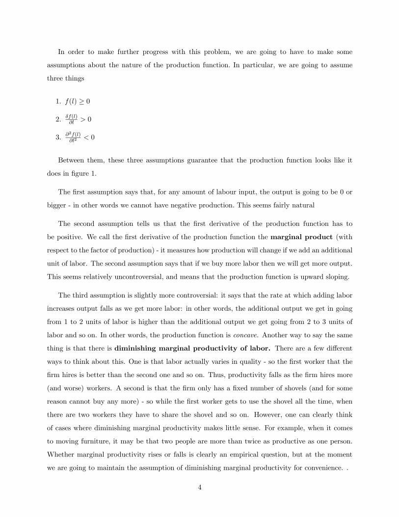
In order to make further progress with this problem, we are going to have to make some

assumptions about the nature of the production function. In particular, we are going to assume

three things

1. () ≥ 0

2.()

0

3.2()

2 0

Between them, these three assumptions guarantee that the production function looks like it

does in figure 1.

The first assumption says that, for any amount of labour input, the output is going to be 0 or

bigger - in other words we cannot have negative production. This seems fairly natural

The second assumption tells us that the first derivative of the production function has to

be positive. We call the first derivative of the production function the marginal product (with

respect to the factor of production) - it measures how production will change if we add an additional

unit of labor. The second assumption says that if we buy more labor then we will get more output.

This seems relatively uncontroversial, and means that the production function is upward sloping.

The third assumption is slightly more controversial: it says that the rate at which adding labor

increases output falls as we get more labor: in other words, the additional output we get in going

from 1 to 2 units of labor is higher than the additional output we get going from 2 to 3 units of

labor and so on. In other words, the production function is concave. Another way to say the same

thing is that there is diminishing marginal productivity of labor. There are a few different

ways to think about this. One is that labor actually varies in quality - so the first worker that the

firm hires is better than the second one and so on. Thus, productivity falls as the firm hires more

(and worse) workers. A second is that the firm only has a fixed number of shovels (and for some

reason cannot buy any more) - so while the first worker gets to use the shovel all the time, when

there are two workers they have to share the shovel and so on. However, one can clearly think

of cases where diminishing marginal productivity makes little sense. For example, when it comes

to moving furniture, it may be that two people are more than twice as productive as one person.

Whether marginal productivity rises or falls is clearly an empirical question, but at the moment

we are going to maintain the assumption of diminishing marginal productivity for convenience. .

4

How do we solve the firm’s optimization problem? Actually, we are going to think of three

different ways of doing so. The first way is akin to the way that we set about solving the consumer’s

problem. There, we wanted to get onto the highest possible indifference curve, subject to being in

the budget set. Here we want to be on the highest profit iso-profit line consistent with being on the

production function.

What do iso-profit lines look like? Well, we know that

= −

so rearranging gives us

=

+

Thus, iso-profit lines are upward sloping, with a slope equal to . Also, moving in a North-

Easterly direction moves us to higher iso-profit lines (as the intercept with the vertical axis is

given by ). Figure 2 shows what iso profit lines look like, and figure 3 shows what the profit

maximizing output is going to look like. As we might suspect (assuming that we have an interior

solution) profit maximization is going to occur at the point of tangency - n this case between the

production function and the iso-profit line. And what is true at the point of tangency? The slope

of the budget line has to equal the slope of the production function. In other words, if ∗ is the

profit maximizing level of labor input, then

(∗)

=

or, put another way, the marginal productivity has to equal the ratio of the wage rate to the

price of the good .

Are our assumptions enough to guarantee an interior solution? Unfortunately not. It could be

the case that the iso profit lines are always steeper than the production function, or that they are

always shallower. In the former case, the firm will want to produce 0 goods, while in the latter

they will want to produce an infinite amount. You will deal with such cases in the homework.

A second way to get to the same conclusion is to just solve the optimization problem directly.

In order to do so, realize that we can turn the constrained optimization problem of the firm into

an unconstrained problem by getting rid of the variable altogether. As soon as we have chosen

5

, we have automatically chosen , as the production function tells us what has to be. Thus, we

can rewrite the problem as

Choose: Levels of input ,

In order to maximize: profits: = ()−

And we know how to solve this using calculus Assuming the second order conditions are satisfied,

then this just means differentiating the profit function and setting the result equal to zero:

=

(()− )

= ()

− = 0

⇒ ()

=

This is, unsurprisingly, the same condition as we have before.

Note that, given our assumptions, the second order conditions will be satisfied, as they state

that, for this to be a maximum, the second derivative has to be negative: in other words

2

2=

2()

2 0

Luckily, if we go back and have a look at the assumptions we made about the production function,

we have already guaranteed that this is the case!

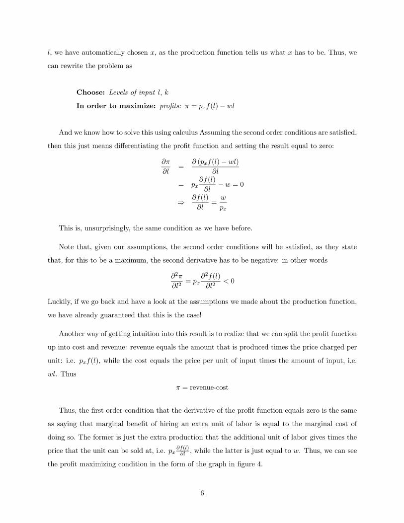
Another way of getting intuition into this result is to realize that we can split the profit function

up into cost and revenue: revenue equals the amount that is produced times the price charged per

unit: i.e. (), while the cost equals the price per unit of input times the amount of input, i.e.

. Thus

= revenue-cost

Thus, the first order condition that the derivative of the profit function equals zero is the same

as saying that marginal benefit of hiring an extra unit of labor is equal to the marginal cost of

doing so. The former is just the extra production that the additional unit of labor gives times the

price that the unit can be sold at, i.e. (), while the latter is just equal to . Thus, we can see

the profit maximizing condition in the form of the graph in figure 4.

6

We can use the graph in figure 4 to also see what will happed to optimal output and labor

as wages and prices change. Figure 5 shows the effect of an increase in the wage rate. This has

the effect of increasing the marginal cost of employing another worker. Remember that, at the

optimum, this has to equal the marginal revenue of employing another worker. Because of our

assumptions about the production function, the firm increases its marginal revenue per worker by

reducing the number of workers, and therefore reducing labor used and output.

We can see this mathematically in the following way. Let ∗( ) be the optimal level of labor

given prices and wages . We know that

(∗( ))

=

so, differentiating by tells us that

2(∗( ))2

∗( )

=1

As 1is positive and

2(∗())2

is negative (by assumption), it must be the case that∗()

is also negative.

Figure 6 shows what happens in the price of the good increases. This raises the marginal

revenue of hiring an extra worker at any given level of production. Thus, in order to make the

marginal revenue of employing another person equal the marginal cost of doing so, the firm has

to increase production, reducing marginal productivity. Again, we can see this mathematically.

Differentiating(∗())

=

with respect to gives

2(∗( ))2

∗( )

= −

2

So, as − 2is negative, and

2(∗())2

is negative,∗()

must be positive.

In order to fix ideas, let us do a specific example: lets assume that () = 12 (you should check

that this satisfies our three assumptions). The profit for employing workers is therefore

= ()−

= 12 −

7

Taking derivatives with respect to gives

=

1

2

− 12 − = 0

⇒ =³ 2

´2This is the optimal amount of labor demand as a function of wages and prices. Plugging this

back into the production function gives us

= () = 12 =

2

This is the supply function, or how much a firm will choose to supply at for any level of prices

and wages. As we would expect, it is upward sloping, so firms will choose to supply more of the

good as prices increase.

We are now going to look at a third way of solving the same problem. Annoying as this may

seem, the insights we get here will come in very handy further down the road. We are going to

solve the firm’s optimization problem by getting rid of , or labor, rather than getting rid of the

amount of the good produced. Remember that

= ()

So it is also the case that

= −1()

where −1 is just the inverse of the demand function (if you are not sure how inverses work,

then the website http://uncw.edu/courses/mat111hb/functions/inverse/inverse.html has a good

description).

Therefore we can rewrite the firm’s profit function as

() = − −1()

Now the first term is the revenue gained from selling units, while the second term is the cost

of producing those units. In fact, we often rewrite −1() as ( ) - the cost of producing

units when the wage rate is , so the profit function becomes

() = − ( )

8

The optimal level of output is found (assuming that the second order conditions are satisfied)

by setting the derivative with respect to to zero:

− ()

= 0

⇒ =()

In other words, the marginal revenue (which we will write as ()) equals the marginal

cost (()) of producing another unit of production.

Note that the terminology gets a bit confusing here, as we have used terms that sound similar to

marginal revenue and marginal cost before. However, then we were talking about marginal revenue

and marginal cost with respect to changes in labor demand in other words, the additional revenue

and cost of employing one more unit of labor. Here, we are talking about marginal revenue and

marginal cost with respect to an extra unit of production - in other words the extra revenue and

cost of producing one more item to sell. If we are being formal, we should always say marginal

revenue and marginal cost with respect to what. However, if it is not specified the people usually

mean with respect to an extra unit of production rather than labor.

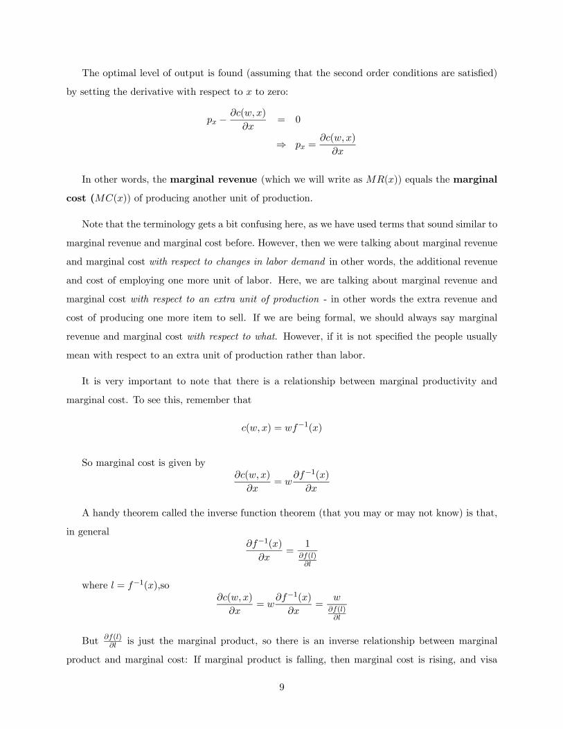
It is very important to note that there is a relationship between marginal productivity and

marginal cost. To see this, remember that

( ) = −1()

So marginal cost is given by

()

=

−1()

A handy theorem called the inverse function theorem (that you may or may not know) is that,

in general

−1()

=1

()

where = −1()so( )

=

−1()

=

()

But()

is just the marginal product, so there is an inverse relationship between marginal

product and marginal cost: If marginal product is falling, then marginal cost is rising, and visa

9

versa. This should also make perfect sense - if the amount we can produce with an additional unit

of labor is falling, then the cost of producing an additional unit of output should be rising.

Our baseline assumption is that()

is decreasing as and increases, which implies that()

increases as increases. The graph of marginal cost and marginal revenue will therefore look like

it does in figure 7.

Going back to our example, in which () = 12 we can see that

= 12

and so 2 = −1() =

The cost function is therefore given by

( ) = −1() = 2

and the production function

= − 2

The first order condition gives us

= − 2 = 0

⇒ =

2

Exactly the same result as when we replaced rather than ..

Another important concept to introduce here is that of the average cost. This is just the

average cost of each unit produced, or

() =()

A couple of interesting things about average costs: First, they are related to marginal costs, in

the following way: If marginal costs are higher than average costs must be rising, and visa versa.

This makes sense: If the cost of an additional unit of production is higher that the average cost of

things produced so far, then it must be the case that average cost is rising. We can see this formally

by noting that

() =()

10

and so

()

=

()

− ()

2

=1

∙()

− ()

¸=

1

[()−()]

Which will be positive if and only if marginal cost is greater than average cost.

The second thing is that profit will be positive if and only if price is greater than average cost.

To see this, note that

() = − ( ) 0

⇒ ()

⇒ ()

= ()

To illustrate some of the above points a little bit more, let’s think of a production function that

breaks one of our initial three assumptions- in particular a production function that is not always

concave. In particular, let’s think about the production function illustrated in figure 8. This shows

a production function that is initially convex, and then becomes concave at higher levels of labor.

- in figure 8 the production function is convex below ∗ and concave above ∗. (One reason to

study such a function is that they are very popular in more basic economic courses).

What does marginal product look like with such a production function? Well, remember that

marginal product is just the slope of the production function, which is always positive. However,

when the production function is convex, marginal product is increasing (i.e. for labor below ∗),

while for values above ∗ it is decreasing. In other words, for values below ∗, labor is becoming

more productive the more is hired, while for values above ∗ it is becoming less productive. This

is shown in figure 9.

Before, we said that profit is maximized when the iso profit lines are tangent to the production

function. However, in this case we are going to get two points of tangency. as shown in figure

10, labelled 1 and 2. Obviously only one of these is profit maximizing. In fact, 1 is a profit

minimizing output.

11

What does marginal cost look like in this case? Well, for output below ∗ (the output given by

∗), marginal product is increasing so, as we have shown above, marginal cost is falling. For output

above ∗, marginal product is falling so marginal cost is increasing. Thus, marginal and average

cost look as they do in figure 11. Note that marginal cost crosses average cost at the bottom point

of its curve (why?).

One very important point is that we need marginal product to start falling at some point if

we are going to be able to solve the firms problem. To see this, note that, if marginal product is

always rising, then marginal cost is always falling - thus a firm who is profitable at a certain level

of output will be even more profitable if they produce more. You will work more with this problem

in the homework.

12

4 The Case of Two Inputs

Now we have dealt with the case where there is only one input into the firm, we will now go back to

the more general (and more interesting) case of two inputs. In other words, the firm’s optimization

problem is once again

Choose: an output level and levels of inputs ,

In order to maximize: profits: = − −

Subject to: the production function = ( )

Once again, we have two potential methods to solve this problem.

Method 1 Substitute in for and make it an unconstrained optimization problem in and . In

other words, choose and to maximize

= − −

= ( )− −

Method 2 Split the problem up into two parts:.

1. Find the cheapest way to produce any amount , and so calculate ( ), or the cost

of producing when rent is and wages are

2. Find the level of output that maximizes

= − −

= − ( )

It turns out that the second approach is going to be easier, provide more insight, and allows us

to use many of the tools that we have already developed, so we will concentrate on that. The other

way, is of course not impossible, and you can try it if you wish.

Taking the second approach, we now have two optimization problems to solve, the first being a

cost minimization problem:

13

Choose: a levels of inputs ,

In order to minimize: costs +

Subject to: attaining some level of output = ( )

We can think of solving this problem graphically, using a graph that has on the horizontal axis

and on the vertical axis. We can then draw iso-cost lines to represent our objective functions, and

an iso-output lines to represent the constraint. As we do so, things should start to look hauntingly

familiar.

First, what do iso cost lines look like? We can get that just from rearranging the following

expression

= +

⇒ =

−

So iso cost lines are straight lines, with slope , and intercept the vertical axis at

as shown

in figure 12. Moreover, we get to lower cost lines as we move in a South-Westerly direction.

What does the constraint look like? This is going to depend on the properties of the production

function. The constraint says that we have to use enough and in order to produce an amount

. We therefore want to draw an iso-output line on our graph, or the collection of and that

produce an output . We are going to make two assumptions about the production function that

should again remind you of something

1. It is monotonic: i.e. for 2 ≥ 1 and 2 ≥ 1 (2 2) ≥ (1 1)

2. It is convex i.e.

For 1 1 2 2 such that (1 1) = (2 2)

and number between 0 and 1

((1 + (1− )2) (1 + (1− )2) ≥ (1 1)

As usual we can define strict monotonicity and strict convexity in the appropriate way.

What do these assumptions mean? Well, the first one is quite intuitive - it just tells us that if we

employ more and then we get (at least weakly) more output. This seems pretty uncontroversial.

14

As usual, the second assumption is a little bit more controversial, but also a little bit more useful.

What this assumption is telling us (roughly) is that we are going to get more production if we

employ 5 units of and 5 units of than if we employ 10 units of and 0 of , or 0 units of and 10

of . In other words, it is more efficient to use ‘average bundles’ of inputs than it is to use extreme

bundles.

What does this imply for our graph of the production function? You should be able to tell

if you realize that the assumptions we just made about the production function are exactly the

same as those that we made about the utility function. Moreover, an iso-output line is exactly the

same as an indifference curve. Thus, our iso output lines are going to look exactly the same as our

indifference curves, in that they are

1. Downward sloping

2. Do not cross

3. Move to higher levels of production as we move in a North Easterly direction

4. Are convex

In fact, we tend to use the same types of function to represent production functions as we do

to represent utility functions namely

1. Cobb-Douglas production functions:

( ) =

2. Perfect compliment production functions (usually called Liontief production functions)

( ) = min( )

3. Perfect substitute production functions

( ) = +

These are illustrated in figures 13, 14 and 15.

15

So the problem is one of figuring out the lowest possible iso cost curve we can get onto, given

that we have to be on a particular iso output line, as illustrated in figure 16. Luckily, this is exactly

the same problem that we have spent ages solving in consumer theory, so we know exactly what we

are trying to do here (yes?). In fact, exactly the same procedure will work here as it did in finding

the optimal bundle for the consumer.

1. Find any points of tangency

2. Calculate the cost of production at the points of tangency

3. Compare to the cost of production at the corner solutions (if corner solutions are possible)

4. Pick the point of tangency or corner solution that has the lowest cost of production

By the same logic we used for the consumer, we know that any solution to this problem has

to be either a point of tangency or a corner solution, so solving this problem is just the case of

choosing the best from this set. The only wrinkle here is that it may, in fact not be possible to

obtain a particular level of output at a corner solution (for example, is it possible to produce 10

units of output using only if the production function is Liontief?)

How do we find points of tangency? Again, the process should be familiar. The point of

tangency is the point at which the slope of the iso-cost line equals that of the iso output line. The

slope of the former is easy - it is just − , or the ratio of the rental rate to the wage rate. What

about the slope of the iso-output line? Remember that all the points along an iso out put line

are combinations of labor and capital that give the same level of output. Thus, the slope of the

iso-output line measures the rate at which you can substitute labor for capital while keeping the

level of output constant (as shown in figure 17). We call this the marginal rate of technical

substitution. Note the parallels between this concept and the marginal rate of substitution that

we discussed in consumer theory. There, we were measuring how we could trade off one good for

another, while keeping the consumer indifferent. Here, we are measuring how we can trade off one

good for another while keeping the level of output constant.

Thus we have our cost minimizing condition (assuming we have an interior solution)

=

16

Where is the marginal rate of technical substitution between labor and capital.

How do we find the marginal rate of technical substitution? A quick think back to the case of

the consumer might lead us to think that it is something to do with the derivative of the production

function with respect to capital and labor. And indeed this is the case. We can see this by totally

differentiating the production function

( ) =( )

+

( )

As, along the iso output curve we know that ( ) = 0, we have

( )

+

( )

= 0

⇒

= −

()

()

=

Thus, the marginal rate of technical substitution is equal to the ratio of the marginal products.

We now know how to find the cost minimizing use of capital and labor with respect to the

parameters of the problem. We will now illustrate this with an example:

Example 1 We want to find the profit maximizing output of a firm that can sell its goods for price

, faces factor prices and and has a production function of the form ( ) = .

The first thing we need to do is find the cost function ( ) of the firm, or in other words

the cost minimizing way of producing goods. As this is a Cobb-Douglas production function we

know that this is going to be an interior solution, and therefore cost minimization will occur at the

point where =. We also know that

()

()

= , so we will begin by taking the

derivative of the production function with respect to labor and capital

( )

= −1

( )

= −1

Taking the ratio of the two marginal products gives us

()

()

=−1

−1=

17

and setting this equal to the ratio of rent to wages gives

=

⇒ =

So this now tells us the ratio of to at the cost minimizing point. But how much and do

we use to produce output ? To figure this out we need to substitute into the production function

( ) =

⇒ =

⇒µ

¶

=

+ =

µ

¶

=

µ

¶ +

1

+

Substituting back in, we get that demand for capital is given by

=

=

µ

¶ +

−1

1+

=

µ

¶ +

1

+

We therefore now know the demand for labor and capital as a function of , and . We will

write these demand functions as

∗( ) =

µ

¶ +

1

+

∗( ) =

µ

¶ +

1

+

But remember what we are really interested in is the cost function. However, this is easy to

calculate, as we know that costs are just given by

( ) = ∗( ) + ∗( )

=

µ

¶ +

1

+ +

µ

¶ +

1

+

=

Ã

+

+

õ

¶ +

+

µ

¶ +

!!

1+

18

This gives us the cost function for our producer.

So we now have solved half the problem for our firm - for any given level of output we can figure

out the cheapest way of producing that level of output. The next thing we need to do is to figure

out the profit maximizing level of output. Recall, this will occur at the point at which price equals

marginal cost, as

() = − ( )

and so, for profit maximization we have

=( )

IF WE HAVE AN INTERIOR SOLUTION.

Recall that, in the case of a single factor of production, we said that to find an interior solution

it had to be the case that marginal costs have to start rising at some point: If marginal costs are

always falling, then the firm will either want to produce 0 or∞. This is also the case with multipleinputs: if the firm is not going to be at a corner solution, we need marginal costs to start rising at

some point.

In the case of a single input, all we needed for marginal costs to start rising was for marginal

product to start falling at some point. Is that enough in the case of multiple inputs? To answer

this, lets have a look at our example. Remember that marginal product of capital is given by

( )

= −1

And so to find out whether the marginal product of capital is increasing or decreasing, we take

the second derivative of the production function:

2( )

2= (− 1)−2

This will be decreasing as long as 1. Similarly, the marginal product of labor will be

decreasing if 1. So, if both and are less than one, is that enough to guarantee that that

marginal cost is rising? Remember that the cost function is given by

( ) =

Ã

+

+

õ

¶ +

+

µ

¶ +

!!

1+

19

For convenience, let’s call

µ

+

+

µ³

´ +

+³

´ +

¶¶= , and note that has to be

positive. So marginal cost is given by

( )

=

1

+

1+

−1

To figure out whether marginal costs are increasing or decreasing, we differentiate again with

respect to , giving

2( )

2=

µ1

+

¶µ1

+ − 1¶

1+

−2

Marginal costs will be increasing as long as

1

+ − 1 0

⇒ 1 +

So we require the sum of and to be less that 1. Thus, it is not enough for marginal product

to be decreasing: if = 075 and = 075 then the marginal product of capital and labor will be

decreasing, but marginal costs will always fall.

So if marginal product is not enough to tell us whether marginal costs are rising or falling,

what is? It turns out, we need to introduce the idea of the returns to scale of a firm. The idea

of returns to scale is to ask the following question. If we doubled the amount of each input into

production, what would happen to output? We can basically think of three cases: Firstly, it could

be the case that doubling the inputs more than doubles the output: This is the case in which a

firm becomes more efficient as it increases in size. Second, it could be the case that doubling the

inputs less than doubles output. This would be the case if the firm were to get less efficient as it

got larger. Alternatively, it could be the case that doubling inputs exactly doubles outputs. In this

case, the size of the firm does not affect its efficiency.

The first of these cases is an example of increasing returns to scale, the second decreasing returns

to scale, the third constant returns to scale. In fact, we define the concepts slightly more generally

than just doubling the inputs, as we can see below:

Definition 1 Let ( ) be the production function of a firm if, for 1

1. We say that the firm exhibits increasing returns to scale if ( ) ( )

20

2. We say that the firm exhibits decreasing returns to scale if ( ) ( )

3. We say that the firm exhibits constant returns to scale if ( ) = ( )

What is the returns to scale of the Cobb-Douglas firm that we used in our example? We can

work this out as follows:

( ) = ()()

= +

= +( )

In other words, the firm will exhibit increasing returns to scale if + 1, decreasing returns

to scale if + 1 and constant returns to scale if + = 1. But if we look back at the

conditions for whether or not marginal costs are increasing and decreasing, we see that marginal

costs are decreasing only if + 1. So in other words, if the firm exhibits decreasing returns to

scale, then their marginal costs will be rising. This will generally be true for the problems we look

at: decreasing marginal product is not enough to guarantee rising marginal costs, but decreasing

returns to scale is.

Now lets carry on with our example, assuming that + 1

Example 2 (Example 1 continued) Now that we have solved the cost minimization problem,

we can solve for the profit maximizing output. Remember that

= − ( )

so the profit maximizing condition is that

= − ( )

= 0

Looking back at the cost function, we see that

( )

=

1

+

1+

−1

And so

=1

+

1+

−1

⇒ =³(+ )

´ +1−−

21

where, by the assumption of decreasing returns to scale, +1−− 0. Having solved for , we

can now plug back into the demand functions for labor and capital to solve for the input demand.

A final issue is the comparative statics of the firm: In other words - how do changes in the

parameters of the problem (, and ) affect the amount of output that the firm chooses to

produce, and its demand for inputs? To answer this question, we are going to pull a new trick:

Lets imagine that 1, 1 and 1 and one set of parameters, and ∗1, ∗1 and ∗1 are the optimal

output and input demands associated with those parameters. Similarly, let 2, 2 and 2 be a

second set of parameters, and ∗2, ∗2 and ∗2 be the optimal response to those parameters. If

∗1,

∗1

and ∗1 are profit maximizing for 1, 1 and 1, then they must give more profit than ∗2, ∗2 and

∗2 for those parameters. In other words

1∗1 − 1

∗1 − 1

∗1 ≥ 1

∗2 − 1

∗2 − 1

∗2

Similarly,

2∗2 − 2

∗2 − 2

∗2 ≥ 2

∗1 − 2

∗1 − 2

∗1

Subtracting the right hand side of the second equation from the left hand side of the first

equation, and the left hand side of the second equation from the right hand side of the top equation

gives

∆∗1 −∆∗1 −∆∗1 ≥ ∆∗2 −∆∗2 −∆∗2

Where ∆ = 1 − 2 and so on. This tells us that

∆∆∗ −∆∆∗ −∆∆∗ ≥ 0

This equation immediately tells us something about the comparative statics of the problem.

First, assume that the price of good increases, but wages and rents do not change. The above

equation tells us that ∆∆∗ ≥ 0, so if ∆ 0, it must be the case that ∆∗ ≥ 0: In other

words, if the price increases then the amount the firm produces will have to increase. Similarly, if

the wage rate goes up, but prices and rents do not change, then the above equation tells us that

∆∆∗ ≤ 0, so if wages go up, then demand for labor must go down.

So far, so sensible. But what is the effect of an increase in prices on factor demand? Or an

increase in the wage rate on output? The results here are slightly less intuitive. Firstly, it can be

22

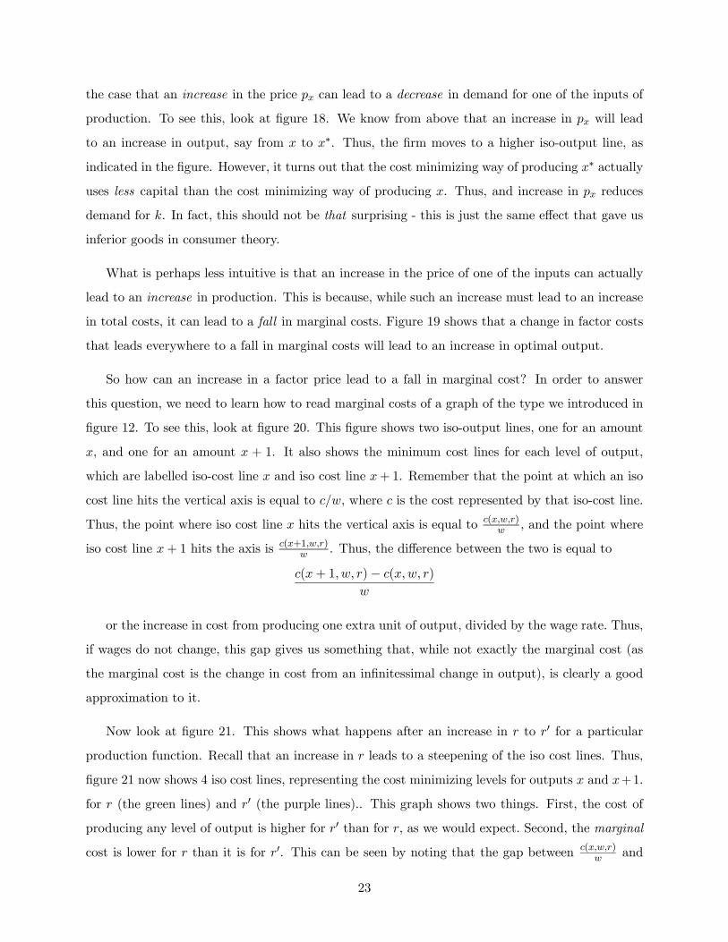
the case that an increase in the price can lead to a decrease in demand for one of the inputs of

production. To see this, look at figure 18. We know from above that an increase in will lead

to an increase in output, say from to ∗. Thus, the firm moves to a higher iso-output line, as

indicated in the figure. However, it turns out that the cost minimizing way of producing ∗ actually

uses less capital than the cost minimizing way of producing . Thus, and increase in reduces

demand for . In fact, this should not be that surprising - this is just the same effect that gave us

inferior goods in consumer theory.

What is perhaps less intuitive is that an increase in the price of one of the inputs can actually

lead to an increase in production. This is because, while such an increase must lead to an increase

in total costs, it can lead to a fall in marginal costs. Figure 19 shows that a change in factor costs

that leads everywhere to a fall in marginal costs will lead to an increase in optimal output.

So how can an increase in a factor price lead to a fall in marginal cost? In order to answer

this question, we need to learn how to read marginal costs of a graph of the type we introduced in

figure 12. To see this, look at figure 20. This figure shows two iso-output lines, one for an amount

, and one for an amount + 1. It also shows the minimum cost lines for each level of output,

which are labelled iso-cost line and iso cost line +1. Remember that the point at which an iso

cost line hits the vertical axis is equal to , where is the cost represented by that iso-cost line.

Thus, the point where iso cost line hits the vertical axis is equal to()

, and the point where

iso cost line + 1 hits the axis is(+1)

. Thus, the difference between the two is equal to

(+ 1 )− ( )

or the increase in cost from producing one extra unit of output, divided by the wage rate. Thus,

if wages do not change, this gap gives us something that, while not exactly the marginal cost (as

the marginal cost is the change in cost from an infinitessimal change in output), is clearly a good

approximation to it.

Now look at figure 21. This shows what happens after an increase in to 0 for a particular

production function. Recall that an increase in leads to a steepening of the iso cost lines. Thus,

figure 21 now shows 4 iso cost lines, representing the cost minimizing levels for outputs and +1.

for (the green lines) and 0 (the purple lines).. This graph shows two things. First, the cost of

producing any level of output is higher for 0 than for , as we would expect. Second, the marginal

cost is lower for than it is for 0. This can be seen by noting that the gap between ()

and

23

(+1)

is larger than the gap between(0)

and

(+10)

. Thus, this is a case in which an

increase in the cost of increases total cost, decreases marginal cost, and so increases optimal

output.

5 When to Pack up and Go Home

Remember that earlier we showed that profits are positive whenever price is higher than average

cost. For the most part, our assumptions thus far have insured that this is always the case, as

marginal cost has always been above average cost, and as profit maximization occurs at the point

at which price is equal to marginal cost, price is definitionally above average cost. However, what

about the case where the production function looks like it does in figure 8? Here, marginal cost

is initially decreasing and then increasing. Moreover, marginal cost will initially be below average

cost, then go above it, as shown in figure 11. In this case it may be that if the firm sets the

price equal to marginal cost they make negative profits. Look at Figure 22. This shows two prices,

1 and 2. At 1, marginal cost equals price at 1, while at 2, price equals marginal cost at 2.

Does the firm make positive profits in both of these cases? The answer is no. at 1, price is below

average cost, so profits are negative, while at while at 2 price is above marginal cost, so profits are

positive. Thus, if price is 1, the firm would be better off producing zero.

What is the minimum price at which the firm will produce a positive amount of output? The

answer is the minimum average cost point, as shown by ∗ in figure 23. At this point, the firm

maximize profits by setting price equal to marginal cost at ∗ (remember that that the marginal

cost line crosses the average cost line at its minimum point) and the firm makes zero profit. At

prices below ∗ then the firm will make negative profit, while at prices above ∗ the firm can make

positive profit. Thus, the supply of such a firm will look like it does in figure 24: at prices below

∗ the firm will produce zero. At prices above ∗ the firm will produce at the point at which price

equals marginal cost.

This analysis has so far assumed that a firm who produces zero faces zero costs. While this

may be a good long run assumption (the firm can always shut down), it may not be such a good

assumption in the short run. For example, if a firm has signed a long term lease on a factory, then

they will have to pay rent on that factory, even if they produce no output. In such a case, it will

be handy to split the cost of the firm into two portions, a fixed cost , which we define as the cost

24

of producing zero output, or (0), and the variable cost of producing , which we will indicate as

(), which we define as () = ()− (0), (from now on we will not write down that and

depend on and , but you should remember that this is the case). Thus, the cost function is now

() = ()− (0) + (0)

= () +

and the profit function

() = − ()−

Note that the addition of the fixed costs does not change the conditions for an interior solution,

as this occurs when

= − ()

= 0

⇒ =()

However, now the firm may be better off producing even if prices are below average cost. To

see this, note that the firm is better off producing at the point of tangency if the profits for doing

so are higher than the profits of producing at zero. But now, the profits for producing at zero are

0− (0)− = − . Thus, the firm will want to carry on producing if

− ()− ≥ −

− () ≥ 0

⇒ ≥ ()

Note that()

is the average variable cost of producing at , which we will denote as ().

Note also that average variable cost is always below average cost, as

() =() +

=()

+

= () +

25

This situation is depicted in figure 25: The firm will keep producing as long as prices are above

the minimum level of average variable cost, as shown by ∗∗. (as you will see in the homework, the

marginal cost curve also crosses the average variable cost curve at the bottom).

This gives us the following theorem

Theorem 1 Let ∗ = min∈ (). Then a firm will produce a positive amount of output if

∗ and produce zero if ∗. If = ∗ then they are indifferent between producing either 0 or

the output at which ) = ∗.

6 Producer Surplus

We have now developed the tools necessary to figure out how much output a firm will produce for a

particular price by solving its optimization problem. When in consumer theory, we decided that we

could gain some information about how good an outcome was for the consumer by looking at the

area under the demand curve. Can we say anything similar about the supply curve? The answer

to this, it turns out is yes.

To see this, we will return to the case where we assume that marginal costs are always rising,

and there are no fixed costs. In this case, the supply curve will not ‘jump’ as it did in the examples

in section 5, and so at every point of thee supply curve, price will equal marginal cost. Thus supply

curve will look like it does in figure.26.

It turns out that the area under the supply curve up to an amount ∗ tells us the cost that the

firm faces in producing ∗. To see, let () be the price associated with the output level by the

supply curve, and remember that along the supply curve

() =() =()

26

Thus, integrating along the supply curve gives usZ ∗

0

()

=

Z ∗

0

()

= [()]∗0

= (∗)− (0)

= (∗)

where the last line comes from the fact that we assumed no fixed costs. Thus the area under

the supply curve equals the total cost of producing ∗. However, the total revenue of producing an

amount ∗ at price ∗ is just equal to ∗∗, or the area under the price line ∗ up to ∗. As profit

equals revenue minus cost, the area between the price line and the supply curve must be equal to

profit, or as we sometimes call it, producer surplus. This is shown in figure 27.

Interestingly, as you will show for homework, this is also true for the cases that we covered is

section 5, so in general we can think of the area between the supply curve and the price line as

being equal to profit

7 Industry Supply

So far we have thought about the case where there is only one firm in the economy. However, this

seems to be a bit of a strong assumption. What would the world look like if we had (say) two

firms? In particular, what would the supply function look like?

To make thinks simple, lets assume that each firm has the same technology. This means the

profit maximizing output of each firm is identical at each price, Lets say that 1() is the amount

that firm 1 would produce at price , and 2() be the amount that firm 2 would produce. Then

the total industry supply at price is given by

() = 1() + 2() = 21()

This is shown in figure 28 for the case where the supply curve does not jump. As you can see,

the industry supply curve will get flatter than the individual firm supply curve. As we add more

firms, the supply curve will get flatter still.

27

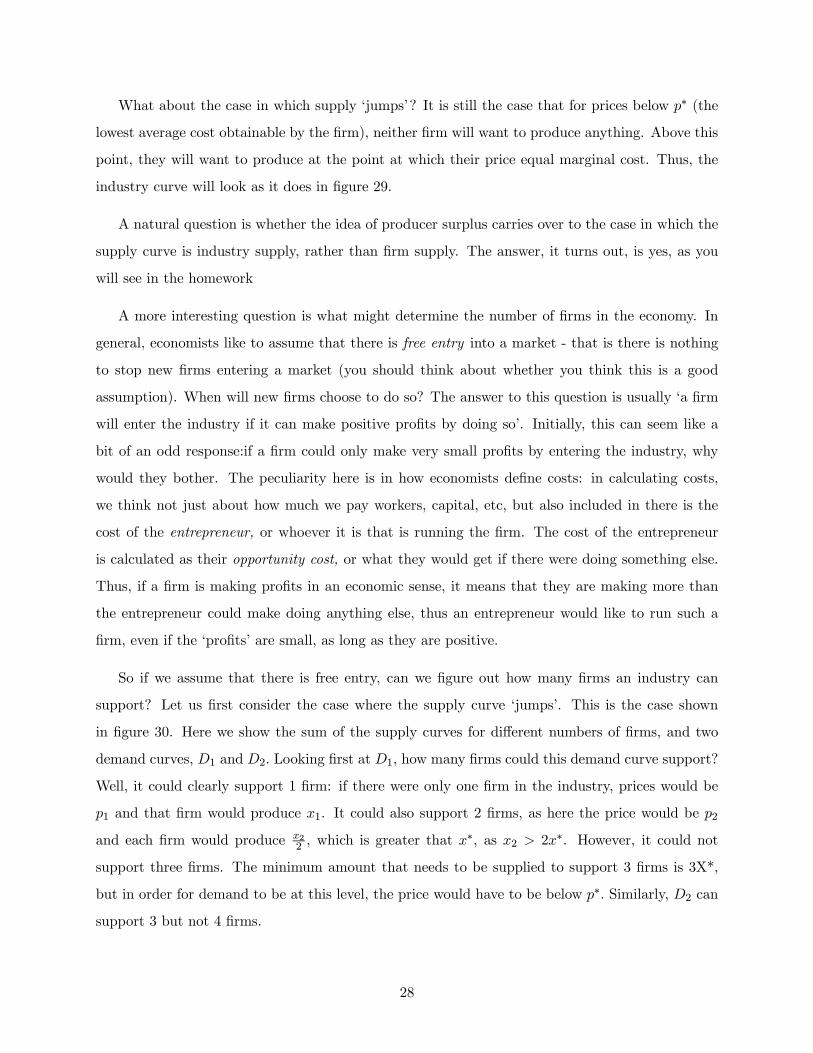
What about the case in which supply ‘jumps’? It is still the case that for prices below ∗ (the

lowest average cost obtainable by the firm), neither firm will want to produce anything. Above this

point, they will want to produce at the point at which their price equal marginal cost. Thus, the

industry curve will look as it does in figure 29.

A natural question is whether the idea of producer surplus carries over to the case in which the

supply curve is industry supply, rather than firm supply. The answer, it turns out, is yes, as you

will see in the homework

A more interesting question is what might determine the number of firms in the economy. In

general, economists like to assume that there is free entry into a market - that is there is nothing

to stop new firms entering a market (you should think about whether you think this is a good

assumption). When will new firms choose to do so? The answer to this question is usually ‘a firm

will enter the industry if it can make positive profits by doing so’. Initially, this can seem like a

bit of an odd response:if a firm could only make very small profits by entering the industry, why

would they bother. The peculiarity here is in how economists define costs: in calculating costs,

we think not just about how much we pay workers, capital, etc, but also included in there is the

cost of the entrepreneur, or whoever it is that is running the firm. The cost of the entrepreneur

is calculated as their opportunity cost, or what they would get if there were doing something else.

Thus, if a firm is making profits in an economic sense, it means that they are making more than

the entrepreneur could make doing anything else, thus an entrepreneur would like to run such a

firm, even if the ‘profits’ are small, as long as they are positive.

So if we assume that there is free entry, can we figure out how many firms an industry can

support? Let us first consider the case where the supply curve ‘jumps’. This is the case shown

in figure 30. Here we show the sum of the supply curves for different numbers of firms, and two

demand curves, 1 and 2. Looking first at 1, how many firms could this demand curve support?

Well, it could clearly support 1 firm: if there were only one firm in the industry, prices would be

1 and that firm would produce 1. It could also support 2 firms, as here the price would be 2

and each firm would produce 22, which is greater that ∗, as 2 2∗. However, it could not

support three firms. The minimum amount that needs to be supplied to support 3 firms is 3X*,

but in order for demand to be at this level, the price would have to be below ∗ Similarly, 2 can

support 3 but not 4 firms.

28

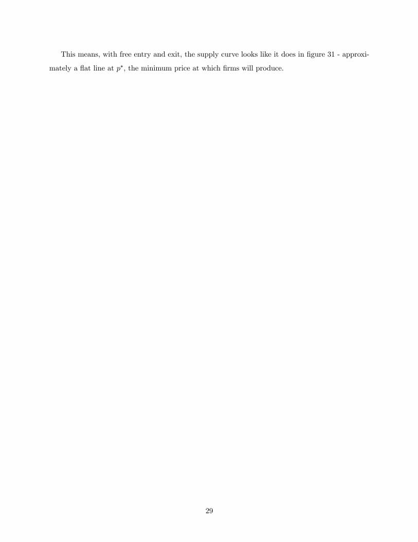
This means, with free entry and exit, the supply curve looks like it does in figure 31 - approxi-

mately a flat line at ∗, the minimum price at which firms will produce.

29

8 Partial Equilibrium

With all the work we have done in the course up until now, we are finally back to where you were in

econ 11: We have a downward sloping demand curve (which we derived in the section on consumer

theory) and an upward sloping supply curve (which we derived above). However, you should not

belittle the work we have done: rather than just being arbitrary lines drawn on the board, we now

have a proper foundation for the supply and demand curves, and a much better understanding of

where these curves come from.

We are now going to use these curves to do some partial equilibrium analysis. In practice,

this means using the supply and demand curves to analyze the effects of various policies, such as

taxes and quotas. The reason we call this partial equilibrium analysis is that we are looking at one

market at a time. Think back to when we did equilibrium in the exchange economy with two goods:

figs and brandy. Changes in one market would implicitly effect what happened in the other market.

Moreover, the welfare of a agents would depend on what happened in both markets. Analysis that

takes this into account is called general equilibrium. Here we are abstracting from that, by

concentration only on one market (say the market for figs). Thus, we are implicitly assuming that

the market we are interested in can be examined in isolation from the rest of the economy.

With that caveat in mind, partial equilibrium analysis can still be extremely useful. The basic

idea is that the market is in equilibrium when prices are such that supply (derived from the firms’s

optimization problem) is equal to demand (as derived from the consumer’s optimization problem).

Thus, figure 32 gives an example of equilibrium in the market for figs.

We can use these diagrams to analyze what would happen to equilibrium prices and quantities

in response to changes in supply and demand conditions. First, let us consider what happens in the

face of a supply ‘shock’. By this I mean a change in conditions which means that firms demand a

higher price to produce any given level of output, or an upward shift in the supply curve. Typically,

people will not be very precise about what it is that causes a supply shock. For example, one could

say that there was a blight on figs trees, reducing the number of fig trees available. But does this

necessarily mean a shift up in the supply curve? Remember that the supply curve is determined

by the marginal cost of producing figs, not the total cost. You should think very carefully about

what sort of changes do imply a shift in the supply curve.

30

Figure 33 shows the effect of a negative supply shock (i.e. an increase in the marginal cost of

production - let’s say due to a blight): this is defined as a shift in the supply curve upwards from

the pre-blight to the post blight line. It should be obvious that equilibrium prices and quantities

shift from 1, 1 to 2, 2, leading to an increase in the price of figs and a decrease in the quantity

of figs produced and consumed.

In contrast, figure 34 shows the effect of a demand shock. This is a shock that effects the

amount that people are prepared to pay for any amount of figs - Figure 34 shows the effect of a

positive demand shock, or an increase in the price that the consumer is prepared to pay for any

level of figs. We will think of this as resulting from a fig festival, when it is traditional for people to

eat figs, but once again you should be very careful about what type of change actually will lead to

a shift in the demand curve. A positive demand shock will lead to an increase in the price of figs

and an increase in the quantity of figs demanded.

We can also use this diagram to do welfare analysis, using the concept of consumer and producer

surplus (are remembering all the caveats we made when constructing these concepts). Remember

that the consumer surplus is given by the area between the demand function and the price line,

while producer surplus is the area between the supply curve and price line as shown in figure 35.

The total of consumer and producer surplus we refer to as total surplus.

We can use the concept of total surplus to analyze the effect of various policies. First, we are

going to think about the effect of an export ban.

Example 3 (Trade Ban) For this example, we are going to thing about the market for miniature

American flags. We will assume that the demand curve for a miniature American flags within the

US is given by

() = 20−

while the supply function is given by

() = 3

Note that, while we are now just writing down demand and supply functions seemingly ar-

bitrarily, we should still think of these as resulting from the optimal decisions of producers and

consumers.

31

We are also going to assume that there is a global market for miniature American flags: On

the global market, consumers can buy as many flags as they want at $4, and producers can sell as

many flags as they want at $4. thus, at $4, global demand and supply is infinitely elastic. This is

a common trick that economists use. The justification is that the global market is ‘large’ relative to

the domestic market, so the amounts demanded or supplied by the US will not have a great effect

on global prices.

How do we analyze this situation using our diagrams. Well, let’s first figure out what demand

and supply would be when the price is $4.

(4) = 20− 4 = 16

(4) = 12

This means, if domestic consumers are allowed to buy on the global market, then the price in

the domestic market will also be $4, domestic demand will be 16 flags, domestic supply will be 12

flags, and the US will import 4 flags, as shown in figure 36. The surplus under this regime is shown

in figure 37, which we can calculate explicitly. Producer surplus is given by

=1

212× 4 = 24

=1

216× 16 = 128

Where these are just the areas of the respective triangles. Total surplus is thus 152.

Now let us analyze the effect of a protectionist policy. A minister decides that, not only is it

unpatriotic to import miniature American flags, it is also harming local workers by suppressing

wages in the miniature flag making industry. Therefore imports should be banned. Following imple-

mentation of the policy, (partial) equilibrium is reached when prices are such that domestic demand

equals domestic supply, (a situation sometimes called autarky). What is this price? We can solve

for it by setting supply and demand equal:

() = 20− = 3 = ()

20 = 4

= 5

And at this price (5) = (5) = 15. This situation is shown in figure 38. We can calculate

32

surplus in this case as

=1

215× 5 = 75

2

=1

215× 15 = 225

2

The policy therefore increases the surplus of producers but reduces the surplus of consumers.

Total surplus is therefore 3002= 150 Thus the policy has lowered total surplus. We can see this

from figure 39, which shows that total surplus falls by an area equivalent to the blue triangle. This

is called deadweight loss, and it should be clear that if the supply curve is upward sloping and the

demand curve is downward sloping we will always have a deadweight loss from such a policy.

Arguments like the above are usually taken by economists to suggest that we should not make

such a change, as there is a loss of efficiency. Because the fall in consumer surplus is larger that the

rise in producer surplus, consumers could afford to compensate producers in order to be allowed

to keep buying at the world price. However, I am not convinced that this is a particularly good

argument. Apart from the problems that we have discussed with consumer and producer surplus,

it is also not the case that it is Pareto dominant to allow trading on the global market. Sure,

there may be a Pareto dominant outcome in which consumers are allowed to trade on the world

market, and then compensate producers, but this seems to very rarely happen in practice (think

second welfare theorem). In fact, one of the effects of globalization seems to have been to bid down

the wages of people who work in export-competing parts of the economy (e.g. manufacturing),

and it is not often the case that such people are compensated for their losses (though note that,

as consumers as well, these people also get to benefit from the lower costs inherent in the world

market).

A second policy we can analyze within this framework is that of a tax

Example 4 (Sales Tax) Imagine that there is no world market for miniature american flags, so

the economy is now at autarky. Some damned American hating socialist decides to implement a $4

tax on each flag sold. What does the (partial) equilibrium look like now? Well, let be the price

that the consumer pays, and be the price that the producer receives. In equilibrium,

() = ()

33

We also know that the difference between these two prices is equal to the tax paid, and so

= + 4. This means we can find equilibrium:

() = ()

( + 4) = ()

20− − 4 = 3

16 = 4

= 4

And so = 8, and () = () = 12This is the situation shown in figure 40.

We can also analyze the welfare effect of this tax. Consumer surplus and producer surplus

obviously fall a lot

=1

212× 4 = 24

=1

212× 12 = 72

However, the picture is not quite as bleak as that,as the government receives some tax revenue.

This is equal to the tax per item times the number of items sold

= 12× 4 = 48

Thus, ‘social surplus’ (i.e. consumer surplus+producer surplus +tax revenue ) is 72+24+48=144.

The deadweight loss of the tax is 6, as illustrated in figure 40.

In this case, the deadweight loss of the tax comes about due to inefficiency: The tax drives a

‘wedge’ between the price that people are willing to pay for a good, and the price that firms would

accept to produce the same good. This is a point that we will come back to.

9 General Equilibrium

Partial equilibrium is certainly a useful concept, but there are reasons why, in the Edgeworth

box, we looked at both markets at the same time. There are important results that only can

34

be derived by thinking of the economy as a whole - the situation we call general equilibrium. In

particular, when thinking about an economy in which there were only consumers we derived the

rather extraordinary result that any competitive equilibrium is pareto optimal. I promised then

that we would show this also to be the case when we introduced production, and now it is time

to come good on that promise. However, as is typical, we are going to do this in a weird and

roundabout way. I am first going to give an example, and then I am going to prove the statement

directly.

Worse still, the example I am going to give is going to seem really weird. It is what we call the

Robinson Crusoe Economy

9.1 The Robinson Crusoe Economy

As we all know, Robinson Crusoe was stranded on an island, and has to subsist on local materials.

What is less well know (except to economists) is that in doing so, he started to behave in a very

odd manner - in fact, he started to suffer from a split personality. In particular, he split himself

into Robinson Crusoe the worker and Robinson Crusoe Inc., a firm. The former was a simple man,

who had preferences over a consumption good (coconuts) and leisure. The coconuts he bought on

the local market, while he sold his labor to the local firm - Robinson Crusoe Inc. The latter was

a dynamic, thrusting firm which bought labor off Robinson Crusoe (the man), used this labor to

get coconuts, and sold these coconuts to Robinson Crusoe (the man) in order to maximize profits.

These profits go to the sole owner of Robinson Crusoe Inc., a man called Robinson Crusoe.

Why on earth am I telling you this ridiculous story? The reason is that this is a way of analyzing

the simplest production economy - one in which there is one consumer (Robinson Crusoe, henceforth

RC), one firm (Robinson Crusoe Inc., henceforth RCI), one input to production (labor) and one

output (coconuts). What we are going to show is that, in this economy, the competitive equilibrium

is pareto optimal, in the sense that it will lead to a combination of labor and coconuts that will

maximize RC’s preferences.

In order to see this, we have to figure out what such a combination looks like. Doing so involves

solving what we call the ‘planners problem’, or imagining that we are a benevolent social planner

who get to choose a bundle of coconuts and leisure in order to maximize RC’s preferences. In other

words, the planner’s problem asks is the following

35

Choose: an output level and levels of input level

In order to maximize: RC’s preferences ( 24− )

Subject to: the production function = ()

Where is the number of coconuts that RC consumes, and is the amount of labor RC spends

looking for coconuts.

In order to solve this problem, we will start by graphing the constraint. This comes from the

production function: We cannot give RC more coconuts than can be produced given the labor he

provides. We will assume that the production function () has all the nice properties that we have

so far assumed, and so it looks like it does in figure 41. Thus, we know that we have to pick a point

somewhere on this line: this is the combination of labor and coconuts that we have to choose from

However, look at the axis on this graph: these measure labor and coconuts. But these are the

same things that RC has preferences over. Thus, we can graph RC’s preferences on the same graph.

What are they going to look like? Well, assuming that they are ‘nice’ (i.e. monotonic in leisure and

coconuts and convex), the indifference curves will look like they do in figure 42 -the ‘mirror image’

of standard preferences (as the bottom axis shows labor or 24-minus leisure, and so is a ‘bad’ with

respect to RC’s preferences).

By now, we should be very used to figuring out how to solve this sort of thing. We want to

locate the point on the production function that is going to allow us to get on the highest of RC’s

indifference curves. This maximum is going to come at the point where the indifference curves are

tangential to the constraint - which in this case is the production function, as shown in figure 43.

And what is true at this point? The slope of the production function is the same as the slope of

the indifference curve. The slope of the production function is just the marginal product of labor,

while the slope of the indifference curve is the marginal rate of substitution between leisure and

coconuts.

Another way to see the same result is by rewriting the planners problem above as an uncon-

strained optimization problem by substituting in of the production function

Choose: a level of input level

In order to maximize: RC’s preferences (() 24− )

36

Now, in order to find the optimum, we simply differentiate the utility function with respect to

leisure, giving

=

−

⇒

=

=

Thus, the ‘pareto optimum’ in this economy occurs at the (unique)1 point on the production

function at which marginal product equals the marginal rate of substitution.

A moment’s thought should tell us that this makes sense. Marginal product is the rate at which

RCI can convert labor into coconuts. The MRS measures the rate at which coconuts can be traded

for leisure while keeping RC indifferent. If, for example, the marginal product was higher than

the MRS, then we could make RC happier by getting him to provide one extra unit of labor. The

increase in coconuts that RC gets as a result (measured by the marginal product) would more than

offset him for the loss of utility as measured by the MRS.

Now we know what the pareto optimum looks like. What does the competitive equilibrium look

like? First, we have to define what a competitive equilibrium is in an economy with production.

In order to do so, start by recalling how we defined a competitive equilibrium in an economy with

only consumers:

Definition 2 (Equilibrium with consumers only) An equilibrium is a consumption bundle for

each consumer and a price such that

1. The allocation is feasible

2. The consumption bundles solve the consumers optimization problem, given the price and initial

allocations

In other words, we figured out an amount of each good to give to each person such that the total

amount we allocated was equal to the amount of that good in the economy (feasibility), and that

at the equilibrium price, those are the amounts that the consumers would have chosen to maximize

their preferences (optimization). Put another way, we found a set of prices such that demand at

those prices equalled supply.

1Question: What assumption have we made that ensures that this point is unique?

37

We can modify this definition to allow for an economy with producers as well as consumers

Definition 3 (Equilibrium with consumers and firms) An equilibrium is a consumption bun-

dle for each consumer, a production decision for each firm and a set of prices such that

1. The allocation is feasible

2. The consumption bundles solve the consumers optimization problem and the production deci-

sion of each firm maximizes profits, given prices

In other words, we tell each firm exactly what to make, using what inputs, and tell each consumer

what to consume, and post a set of prices such that feasibility is satisfied, and the consumption

bundles and production decisions are exactly what the consumers and firms would have chosen to

do, given those prices.

One question you should ask is: what does feasibility mean when we have production? Well

think of our Robinson Crusoe economy. Here there are two ‘goods’: labor and coconuts. The only

supply of labor comes from RC, while the only demand for labor comes from RCI. In contrast, the

only demand for coconuts comes from RC, while the only supply comes from RCI. Thus, feasibility

means that the amount of labor used by RCI is equal to the amount of labor supplied by RC, while

the amount of coconuts produced by RCI is equal to the amount eaten by RC. You can generalize

the notion of feasibility to a case where there are more firms, more consumers, more goods and

more inputs: feasibility means that, for each input, total amount used by all firms is equal to the

total amount supplied by all households, while for each good, total amount consumed by all the

consumers is equal to the total amount supplied by all the firms.

Returning to our Robinson Crusoe economy, another way to think about the an equilibrium is

that we are looking for a set of prices such that two things are true:

1. The demand for labor by RCI is equal to the supply of labor from RC.

2. The demand of coconuts from RC is equal to the supply of coconuts from RCI

What will the competitive output look like? Lets start by thinking about the behavior of a firm

when the wage rate is (we will normalize the price of coconuts to 1). We know that the firm will

38

choose to produce at the point where the iso profit line is tangential to the production function.

Remember that the iso profit line is given by

= +

So the firm will choose to produce at the point where marginal product is equal to , and the

profit that the firm earns is given by the intercept of the iso cost line with the vertical axis. We

will call the associated demand for labor, supply of coconuts, and profits (), () and ()

respectively. This situation is shown in figure 44. As we know, the marginal product has to equal

the wage rate at this point, so:

(())

=

Note also that the point at which the tangential iso-profit line hits the vertical axis is the profit

that the firm makes.

How about the consumer, RC? First of all, what is RC’s income? This comes from two sources:

the wages that he gets from selling labor (()), and the profits he gets from owning RCI (())If

he is to consume all his income, then the number of coconuts that he buys has to be equal to this

income, so his constraint is

= () +

Does this look familiar? It should, as this is exactly the same as the equation of the iso-cost

line going through the firm’s profit maximizing output. Amazing!

Given this constraint, what will RC choose to consume? As usual, he will choose to consume

at the point at which the budget constraint is tangential to his indifference curves, as shown in

figure.45. We will denote the demand for coconuts and supply of labor that RC would choose as

() and () respectively. And at this point, we know the marginal rate of substitution between

leisure and coconuts is equal to the slope of the budget constraint, so

=()()

So does the wage rate that we have chosen here support an equilibrium? The answer is

no, as shown in figure 46.At the wage rate we have chosen, then RC’s demand for coconuts is

larger than RCI’ supply (() ()) and RC’s supply of labor is greater than RCI’s demand

(() ()).

39

For the wage rate to support an equilibrium, it has to look like it does in figure 47. Here, wage

rate ∗ is such that where (∗) = (∗) and (

∗) = (∗), or the labor that RC wants to

supply is equal to the labor that RCI demands, and the coconuts that RC demands are equal to

the coconuts that RCI supplies.

But note that something else is true about this point. At the equilibrium, we know that the

slope of the indifference curve is equal to the wage rate

∗ =(∗)(∗)

and we know that wage rate is equal to marginal productivity:

((∗))

= ∗

Putting these two together gives

((∗))

=(∗)(∗)

But (gasp!) this is exactly the same condition as we had for the pareto optimum! The com-

petitive equilibrium is the one that maximizes RC’s utility! The first fundamental theorem goes

through! We’re Saved!

What is driving this extraordinary result? It turns out that once again, prices are acting as

devices that equalize marginal rates, and this is the condition that we need to ensure optimality:

When behaving competitively, the firm sets the rate at which it can convert labor to coconuts equal

to the wage rate. Similarly, the consumer sets the rate at which they convert labor into coconuts

at the wage rate. Thus, the equilibrium equilibrates these two marginal rates, which is what we

need for an equilibrium.

Given that the Robinson Crusoe economy is even more specific than some others that we have

looked at, you might be a bit suspicious about this result . Is this true if we have more than one

consumer and more than one firm? Have I pulled a fast one by focussing in Mr. Crusoe? The

answer is no: Production economies generally satisfy the first fundamental welfare theorem, as we

now show. For simplicity we will think of the case where there are two goods in the economy and

, and two inputs into production and . The game we are going to play is look at a competitive

allocation in the economy, which consists of the following objects:

40

1 1, 1, 1 the good consumed and factors of production sold by person 1

2 2, 2, 2 the good consumed and factors of production sold by person 2

, ,, the amount produced and the inputs used by the firm producing

, ,, the amount produced and the inputs used by the firm producing

and consider another allocation (which we will indicate by putting stars in front of everything)

that pareto dominates the competitive allocation. We will show that this new allocation must be

infeasible.

Let’s start off by thinking of the budget constraint of individual 1 at competitive equilibrium:

1 + 1 = 1 + 1 + +

1 and 1 are the amount of and that 1 consumes, while 1 and 1 are the amount of labor

and capital that they produce. is person 1’s share of the firm that produces , while is their

share of the firm that produces . Now, note that, if there was another bundle of inputs and outputs

that 1 could supply ∗1, ∗1 ∗1,

∗1 that 1 would prefer, then they would not be able to afford it, so

it would have to be the case that

1 + 1 − 1 − 1

∗1 +

∗1 − ∗1 − ∗1

Therefore, if we add across the two individuals in the economy, we get

(1 + 2) + (1 + 2)− (1 + 2)− (1 + 2) = +

And, for any pareto improving bundle, it must be that

(∗1 + ∗2) + (

∗1 + ∗2)− (∗1 + ∗2)− (∗1 + ∗2)

(1 + 2) + (1 + 2)− (1 + 2)− (1 + 2)

Now what about the profits of the two firms? These are given by

= − −

= − −

41

Again, as the firms are maximizing profits, then it has to be that these profits are higher than

under the alternative plan, so

− − ∗ − ∗ − ∗

− − ∗ − ∗ − ∗

Adding these two together tells us that

+ − ( + )− ( + )

∗ +

∗ − (∗ + ∗)− (∗ + ∗)

As the competitive allocation was feasible, we know that

(1 + 2) =

(1 + 2) =

(1 + 2) = ( + )

(1 + 2) = ( + )

and so

(1 + 2) + (1 + 2)− (1 + 2)− (1 + 2)

= + −( + )− ( + )

implying that

(∗1 + ∗2) + (

∗1 + ∗2)− (∗1 + ∗2)− (∗1 + ∗2)

∗ +

∗ − (∗ + ∗)− (∗ + ∗)

Rearranging this expression tells us that feasibility must fail, as

(∗1 + ∗2 − ∗ )

+(∗1 + ∗2 − ∗ )

+(∗1 + ∗2 − ∗ + ∗)

+(∗1 + ∗2 − ∗ + ∗)

0

42

10 Externalities

We are now going to return to a topic which we have touched on before: externalities. We discussed

this in the context of equilibrium in the consumer economy, where we described externalities as

a circumstance in which the consumption of one good by one person directly affected the utility

of another. Now we have firms, we can more generally think of externalities as a case in which

the economic activity of one economic agent (firm or consumer) directly affects another. As was

the case with the consumer based economy, this can lead to the competitive equilibrium being

inefficient.

We are going to start with a classic example: pollution. In particular, we are going to think of

two industries: Stan’s Tannery and Ian’s Aromatherapy Spa. Stan’s Tannery is upwind of the spa,

thus, if Stan is producing leather, then Ian is affected by the smell. In particular, we are going to

assume that Ian can still do aromatherapy, but it costs him more, due to the need for more candles

to hide the smell. The more that Stan produces, the more that Ian has to spend. Thus, the profits

of the two firms are given by

= − ()

= − ( )

Where, the first line is the profits for the tannery and is the amount the tannery produces,

while the second line is the profits for the aromatherapy spa, with being the amount of aro-

matherapy that Ian does. What makes this problem non-standard is the fact that ( ), the cost

of aromatherapy, depends on . We have also assumed that

( )

0

What output of tanned goods and aromatherapy will maximize producer surplus, in terms of

the total profits of the two industries? (I know that isn’t the same as welfare, but this is an easy

way of making the point). Joint profits are given by

+ = − () + − ( )

43

Thus, taking first order conditions gives

( + )

= − ( )

= 0

⇒ =( )

and

( + )

= − ()

− ( )

= 0

⇒ =()

+

( )

Thus, the optimal thing in terms of producer surplus is for tanned goods to be produced up

to the point where the price of tanned goods is equal to the marginal cost of producing tanned

goods, plus the marginal effect of producing tanned goods on the cost of aromatherapy. Assuming

that (), this is a situation depicted in figure 47, with a welfare maximizing output of ∗.

What will Stan actually choose to produce? He will, of course, choose the profit maximizing

output for his firm, and so set price equal to marginal cost:

()

= − ()

= 0

⇒ =()

A situation depicted in figure 48. The profit maximizing output is higher that the social

optimum, because Stan does not take into account the effect of his tanning on Ian’s Aromatherapy.

What is to be done? Two possible solutions are

1. Tax the production of leather, as shown in figure 49

2. Force the two firms to merge. Then the single owner will try and maximize total profits, and

so take into account the effect of the tannery on the aromatherapy business.

44