CS534-Machine learning

Perceptron

A Canonical Representation• Given a training example: (<x1, x2, x3, x4>, y)• Transform it to canonical representation

(<1, x1, x2, x3, x4>, y)

• Learn a linear function g(x,w) =w x, where w = <w0, w1, w2, w3, w4>

• Each w corresponds to one hypothesis

h(x) = sign(g(x,w))• A prediction is correct if yw x>0• Goal of learning is to find a good w

– e.g., a w such that h(x) makes few mis-predictions

}1,1{y

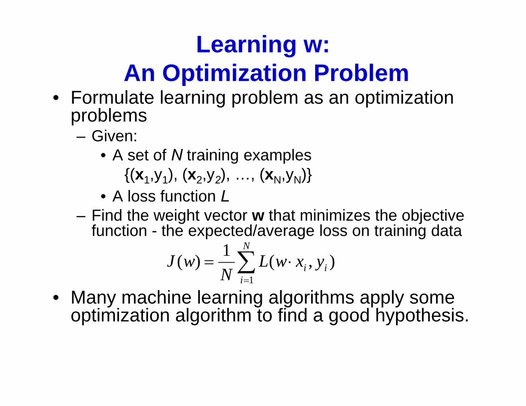
Learning w: An Optimization Problem

• Formulate learning problem as an optimization problems– Given:

• A set of N training examples{(x1,y1), (x2,y2), …, (xN,yN)}

• A loss function L– Find the weight vector w that minimizes the objective

function - the expected/average loss on training data

• Many machine learning algorithms apply some optimization algorithm to find a good hypothesis.

N

iii yxwL

NwJ

1),(1)(

• Start with initial w = (w0,..., wn)• Compute gradient

• , Where is the “step size” parameter• Repeat until convergence

Gradient Descent Search

0))(,,)(,)(()(10

0 wwwwwnw

Jw

Jw

JJ

Remaining question: what objective to use?

Loss Functions• 0/1 Loss function:

L(y’,y) = 0 when y’=y, otherwise L(y’,y)=1• Does not produce useful gradient since the surface of J is flat

0/1 loss

N

iii yxwL

NwJ

11/0 )),(sgn(1)(

Loss Functions• Instead we will consider the “perceptron criterion” (a slightly

modified version of hinge loss):

• The term is 0 when yi is predicted correctlyotherwise it is equal to the “confidence” in the mis-prediction

• Has a nice gradient leading to the solution region

N

iiip xwy

NwJ

1),0max(1)(

0/1 loss Perceptron criterion

),0max( ii xwy

Stochastic Gradient Descent

• The objective function consists of a sum over data points---we can update the parameter after observing each example

• This is referred to as Stochastic gradient descent approach

otherwise

0 if 0otherwise

0 if 0),0max()(

),0max(1)(1

ii

iii

iji

ii

j

i

iii

N

iii

yy

J

xyy

wJ

yJ

yN

J

xxw

xwxww

xww

After observing x , , if it is a mistake w ← w x

Online Perceptron Algorithm

ii

ii

ii

ii

y · uy

· u , yi

xww

xwx

w

0 if

)(: example iningAccept traRepeat

...,0)(0,0,0, Let

Online learning refers to the learning mode in which the model update is performed each time a single observation is received.

Batch learning in contrast performs model update after observing the whole training set.

w1

w2

w3

Decision boundary 1

Decision boundary 2

Decision boundary 3

+

+

-

-

-

-

+

+

Red points belong to the positive class, blue points belong to the negative class

When an error is made, moves the weight in a direction that corrects the error

Batch Perceptron Algorithm

|| until

/

0 if

do to1for ...,0)(0,0,0,

do...,0)(0,0,0, Let

,...,1)( examples training:Given

deltadelta

Ndeltadeltaxydeltadelta

· uy · u

N i delta

N, i , y

ii

ii

ii

ii

ww

xw

wx

Simplest case: η = 1 and don’t normalize – ‘Fixed increment perceptron’

η – the step size

• Also referred as the learning rate• In practice, recommend to decrease η as

learning continues• Some optimization approaches set step-

size automatically, e.g., by line search, and converge faster

• If linearly separable, there is only one basin for the hinge loss, thus local minimum is the global minimum

Online VS. Batch Perceptron• Batch learning learns with a batch of examples collectively• Online learning learns with one example at a time• Both learning mechanisms are useful in practice• Online Perceptron is sensitive to the order that training examples are

received• In batch training, the correction incurred by each mistake is

accumulated and applied at once at the end of the iteration• In online training, each correction is applied immediately once a

mistake is encountered, which will change the decision boundary, thus different mistakes maybe encountered for online and batch training

• Online training performs stochastic gradient descent, an approximation to real gradient descent, which is used by the batch training

Convergence Theorem (Block, 1962, Novikoff, 1962)

.)/(most at is makesalgorithm perceptron that themistakes ofnumber then the

, allfor 0 and 1 , and , , If.),( ... ),,(),,( sequence example ningGiven trai

2

2211

D

iyDiyyy

iii

NN

xuuuxxxx

Note that ||·|| is the Euclidean length of a vector.

Proofamount boundedlower aby ector solution v a closer totor weight vec

the moves updateeach that show toneedjust wee,convergenc show To

factor scalingarbitrary an is where ector,solution v a is given that ector,solution v a also is that Note

uu

kkk ykk xwwx )()1( have wemistake, kth the be Let

kT

k

Tkkk

Tkk

Tk

Tkk

kkT

kT

kk

kkkk

kkkk

yDkkyk

DDykykykyk

ykykykyk

k

xuuwwxxuuw

xxuwxuwxxuwxuw

xuwxuwxuwuxw

uw

because , 2)(0)( because, D2)(

because,2)(2)(2)(2)(

)(])([2)()()(

)1(

22

22

22

22

222

22

2

2D set can wefactor, scalingarbitrary an is Because

222 )()1( Dkk uwuw

Proof (cont.)

22222222 )1()1( kDkDkDk uuwuw

thatshow can we, on inductionBy k

)/(

)(

0

2

2

2

2

22

Dk

DD

k

kD

Margin• is referred to as the margin

– The minimum distance from data points to the decision boundary

– The bigger the margin, the easier the classification problem is

– The bigger the margin, the more confident we are about our prediction

• We will see later in the course this concept leads to one of the recent most exciting developments in the ML field – support vector machines

Not linearly separable case

• In such cases the algorithm will never stop! How to fix?

• Look for decision boundary that make as few mistakes as possible – NP-hard!

Fixing the Perceptron• Idea one: only go through the data once, or a fixed

number of times

• At least this stops• Problem: the final w might not be good e.g. right before it

stops the algorithm might perform an update on a total outlier

ii

ii

ii

ii

y · uy

· u , yi

xww

xwx

w

0 if

)(: example traininga Take timesNfor Repeat

...,0)(0,0,0, Let

Voted Perceptron• Keep intermediate hypotheses and have them vote

[Freund and Schapire 1998]

N

n

Tnnc

0)}sgn(sgn{ xw

Store a collection of linear separators w0 w1 …, along with their survival time c0, c1 …

The c’s can be good measures of the reliability of the w’s

For classification, take a weighted vote among all separators:

Summary of Perceptron• Learns a Classifier ŷ = f(x) directly• Applies gradient descent search to optimize the hinge

loss function– Online version performs stochastic gradient descent

• Guaranteed to converge in finite steps if linearly separable– There exists an upper bound on the number of corrections

needed– Inversely proportional to the margin of the optimal decision

boundary

• If not linearly separable, use voted perceptrons

Geometric Interpretation of Linear Discriminant Functions

The signed distance (positive if x is on the positive side, negative otherwise) from any point x to the decision boundary is:

wx)(y

w0w

Note that in Perceptron, due to the adoption of the canonical representation, all training points will lie on the hyperplane x0=0, and the decision boundary will always go through the origin.