penning ionization of small molecules by metastable neon
TRANSCRIPT

PENNING IONIZATION OF SMALL MOLECULES
BY METASTABLE NEON
by
Joseph H. Noroski
B.S., University of Pittsburgh, 1993
M.S., University of Pittsburgh, 2001
Submitted to the Graduate Faculty of
Arts and Sciences in partial fulfillment
of the requirements for the degree of
Master of Science
University of Pittsburgh
2007

UNIVERSITY OF PITTSBURGH
COLLEGE OF ARTS AND SCIENCES
This thesis was presented
by
Joseph H. Noroski
It was defended on
March 23, 2007
and approved by
Kenneth Jordan, Professor, Chemistry
David Pratt, Professor, Chemistry
Thesis Director: Peter E. Siska, Professor, Chemistry
ii

PENNING IONIZATION OF SMALL MOLECULES BY METASTABLE NEON
Joseph H. Noroski, M.S.
University of Pittsburgh, 2007
Penning ionization electron spectroscopy (PIES) in crossed, supersonic molecular beams was
used to examine the reactions of Ne* (2p53s 3P2, 3P0) with two target molecules, CO2 and C2H2.
Tentative peak assignments were made for each reaction, and the collision dynamics of these
reactions were also examined at various collision energies in light of the two potential model of
Penning ionization. The 2.6 − 3.2 eV region of the Ne* + CO2 spectrum is assigned to a nν1
progression. The region from 2.6 − 2.0 eV is more complex, but a nν1 + 2ν3 progression in
addition to the nν1 progression is very likely present. The region below 2.0 eV contains a broad
band of signal, but no assignments have yet been made on this region. The Ne* + C2H2
spectrum has a very well resolved ν2 progression around 5 eV. The A state of the Ne* + C2H2
PIES spectrum is present, but it can’t be resolved with our data. The Ne* + CO2 reaction was
run at collision energies of 1.73, 1.97, 2.56, and 3.13 kcal/mol. A red shift (~ −18 meV) was
found for all but the 3.13 kcal/mol energy, which was blue shifted (~ 18 meV). This small shift,
combined with broad peakshapes, indicates that ionization occurs over the positive and negative
regions of the Ne* + CO2 potential energy surface, that is, ionization straddles the zero-crossing
point. The Ne* + C2H2 reaction was run at collision energies of 1.80, 2.37, and 2.94 kcal/mol.
A decreasing blue shift with increasing collision energy was found (~ 60, 50, and 45 meV,
iii

respectively). Decreasing blue shift with increasing E is not typical and could be due to
changing dynamic factors as E increases. Since the shift is significantly smaller for Ne* + CO2
than for Ne* + C2H2, we propose that the interaction between Ne* and CO2 is less repulsive than
that of Ne* and C2H2 in the range of geometries over which ionization occurs.
iv

TABLE OF CONTENTS
1.0 PENNING IONIZATION.............................................................................................. 1
1.1 PREVIOUS RESEARCH...................................................................................... 1
1.2 THE TWO POTENTIAL MODEL ....................................................................... 4
2.0 EXPERIMENTAL ....................................................................................................... 13
2.1 VACUUM SYSTEM........................................................................................... 13
2.2 GAS INTRODUCTION ...................................................................................... 15
2.3 ANALYZER, LENS, AND MULTIPLIER ........................................................ 18
3.0 RESULTS AND ANALYSIS...................................................................................... 23
4.0 CONCLUSIONS.......................................................................................................... 39
APPENDIX .................................................................................................................................. 43
BIBLIOGRAPHY ........................................................................................................................ 50
v

LIST OF TABLES
Table 1. Metastable gas atom characteristics.................................................................................. 2
Table 2. Adiabatic ionization potentials of some small molecules............................................... 24
vi

LIST OF FIGURES
Figure 1. The relative velocity vector diagram for a crossed beams experiment. νrel is given by νrel = νmp(A*) − νmp(B) in order to abide by the convention that νrel should point in the direction of the atomic beam in an atom-molecule system. vmp is the most probable velocity of gas particle A or B. The calculation of vmp is shown in detail in the Appendix. .............................................. 5
Figure 2. The two potential model for PI. The flat region (R → ∞) of V+ is exaggerated to aid in visualization of the importance of the difference ε(Ri) − ε0 to our extraction of dynamical information from PIES experiments. The appearance of the well in V+ in the actual case is not so sudden. ............................................................................................................................................ 6
Figure 3. The five regions of our crossed beams PIES instrument............................................... 14
Figure 4. The electrostatic analyzer and einzel lens. Side plates are not shown. ........................ 19
Figure 5. Lens voltages as applied to focus an electron of initial kinetic energy K0 = 4.5 eV. The kinetic energy K at any point along the electron’s path can be obtained from the formula K = K0 – eV. K0 is the kinetic energy of an ejected electron, e is the unit of charge (negative for an electron), and V is the applied voltage. While K will change as the electron travels through the lens, the electron will emerge from the lens with K = K0. ............................................................ 19
Figure 6. Ne*(40 °C) + CO2 + HeI calibration. The vertical lines indicate the literature peak positions for the PES adiabatic transitions for the A, B, and C states of CO2
+. Our peaks for these transitions are red-shifted by 0.14 eV. See the text. The accepted values for the adiabatic transitions are given by subtracting the values in Table 2 from 21.21804 eV.............................. 26
Figure 7. Energy corrected Ne*(40 °C) + CO2 PIES spectrum. ε is the kinetic energy of the ejected electrons............................................................................................................................ 26
Figure 8. Energy corrected PIES spectra for Ne* + CO2 at four collision energies. ε is the kinetic energy of the ejected electrons. The collision energies are in kcal/mol. Each circle represents the sum of the counts at each kinetic energy. The data points are separated by 0.0195 eV. The spectra have been normalized to the same peak intensity and their baselines shifted for display. E is the collision energy in kcal/mol............................................................................................. 28
vii

Figure 9. Energy corrected PIES spectra for Ne* + CO2 at four collision energies. Each circle represents the sum of the counts at each kinetic energy. The data points are separated by 0.0195 eV. The spectra have been normalized to the same peak intensity and their baselines shifted for display. E is the collision energy in kcal/mol. The dark pitchfork shows the location of the 3P2 (n00) progression, based on PES data in Tables 1 and 2. The light pitchfork shows the location of the 3P0 (n00) progression, based on PES data in Tables 1 and 2. The shift of the peaks relative to these values gives us dynamical information about the Ne* + CO2 reaction. See the text. .... 29
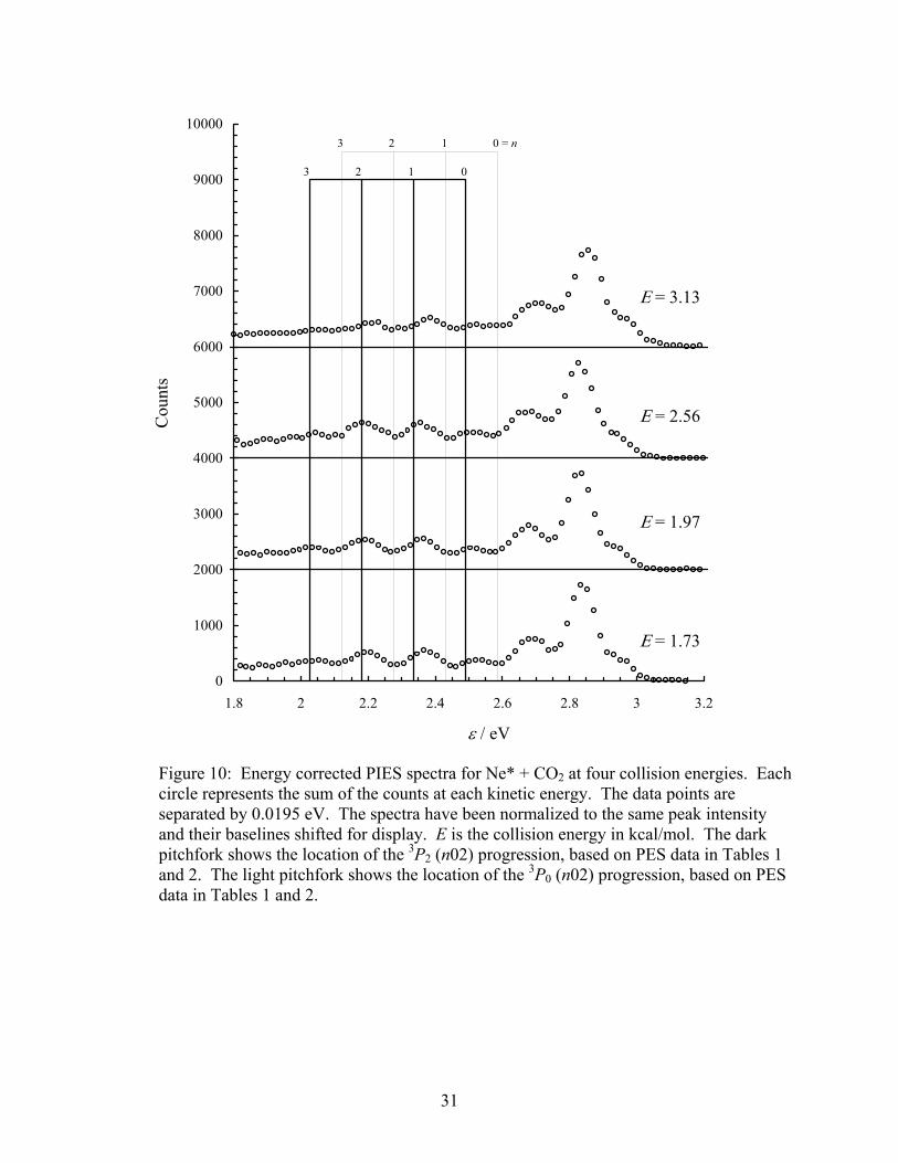
Figure 10. Energy corrected PIES spectra for Ne* + CO2 at four collision energies. Each circle represents the sum of the counts at each kinetic energy. The data points are separated by 0.0195 eV. The spectra have been normalized to the same peak intensity and their baselines shifted for display. E is the collision energy in kcal/mol. The dark pitchfork shows the location of the 3P2 (n02) progression, based on PES data in Tables 1 and 2. The light pitchfork shows the location of the 3P0 (n02) progression, based on PES data in Tables 1 and 2.............................................. 31
Figure 11. Ne*(40°C) + C2H2 + HeI calibration. The vertical lines indicate the literature peak positions for the PES adiabatic transitions for the X and A states of C2H2
+. The accepted values for the adiabatic transitions are given by subtracting the values in Table 2 from 21.21804 eV. Only the X state can be resolved for calibration purposes. See the text. (In some cases, for convenience, the notation A 2
g+Σ ← 1
g+Σ has been used, but this is only true for D∞h symmetry,
which the A state ion does not possess.[35])................................................................................. 33
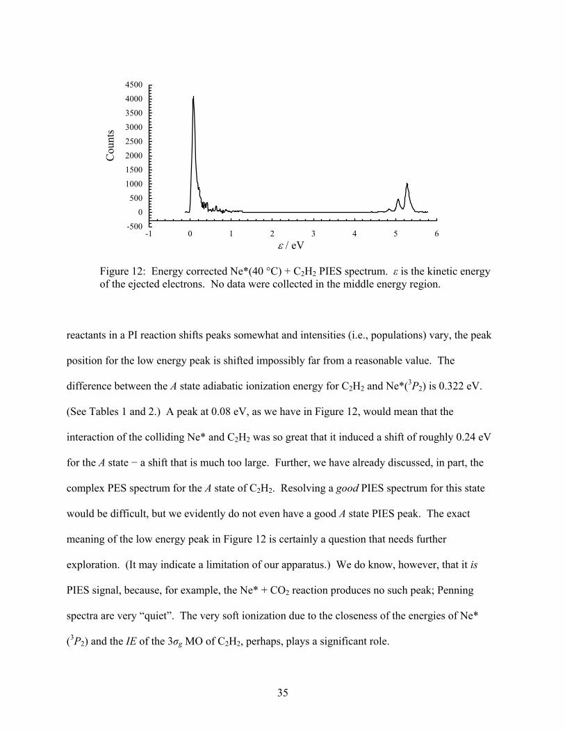
Figure 12. Energy corrected Ne*(40 °C) + C2H2 PIES spectrum. ε is the kinetic energy of the ejected electrons. No data were collected in the middle energy region....................................... 35
Figure 13. Energy-corrected X state spectra for the PIES Ne* + C2H2 reaction at three collision energies. Each circle represents the sum of the counts at each kinetic energy. The data points are separated by 0.0195 eV. The spectra have been normalized to the same peak intensity and their baselines shifted for display. E is the collision energy in kcal/mol. The dark pitchfork indicates the 3P2 (0n000) progression, based on PES data in Tables 1 and 2. The light pitchfork indicates the 3P0 (0n000) progression, based on PES data in Tables 1 and 2............................... 37
viii

1.0 PENNING IONIZATION
1.1 PREVIOUS RESEARCH
Penning ionization (PI) can be represented by A* + B → A + B+ + e–. A* is usually a metastable
atom but, sometimes, it is a molecule. A* is produced by bombarding A with an electron beam.
The Siska group is primarily interested in the reactions for which the metastable atom is a noble
gas. B is the target molecule of our choice. Cermak and Herman1 (1965) were among the first
to suggest determining the kinetic energy of the electrons that are ejected via PI as a means of
monitoring gas phase reactions. This type of experiment is dubbed Penning ionization electron
spectroscopy (PIES).
PIES experiments involving Ne* were first done, of course, with simple target
molecules2: He*, Li, Na, Ar, K, Kr, Xe, Cs, and H2. Many of these experiments were performed
in the 1980’s. Progress in this field, particularly with Ne*, has been slow for three main reasons.
First, the number of scientists initially in this area was small and reduced funding has made that
number even smaller. Clearly, pragmatic concerns influence greatly the direction of scientific
research. Second, the assignment of peaks becomes much more difficult as the number of atoms
in the target molecule increases since there are more molecular orbitals (MO’s) from which
electrons can be ejected and there are more normal modes of vibration that can be excited. Any
1

mixing of these normal modes complicates the electron spectrum even more. Third, Ne* does
not “pack the same punch” as He*, preventing Ne* from probing as deeply into the innards of
target molecules and from ejecting high kinetic energy electrons, which are easier to detect since
they are far from the noise prevalent at low kinetic energy. See Table 1.
Table 1: Metastable gas atom characteristics3
Atom Electron Configuration State
Excitation
Energy (eV)
He
1s2s
2 1S0
20.6158
2 3S1 19.8196 Ne 2p53s 3 3P0 16.7154
3 3P2 16.6191
Nonetheless, some wayward, yet intrepid, physical chemists persist in this area. B.
Lescop et al.4 (1998) examined the PI of CO2 by Ne*, made peak assignments, and proposed a
non-van der Waals interaction between the colliding species. Maruyama5 et al. (2000) examined
the PI of CO2 clusters by Ne*. Additionally, the B. Lescop and F. Tuffin group has
explored6,7,8,9,10 via PIES the reactions of Ne* with NH3, C2H2, H2O, N2, and CO. By
comparison to NeI photoionization the NH3 results showed that Ne*/NH3 interaction influences
the ionization dynamics and, in typical fashion, they explored the agreement of vibrational
populations with Franck-Condon factors. Vecchiocattivi (1990) et al.11 have also conducted
crossed beam studies of excited neon on many small molecules to determine total ionization
cross sections. Only recently has the Vecchiocattivi group configured their apparatus to perform
2

kinetic energy studies in the manner that P. E. Siska mastered in ages past. See below. In a
study12 (2005) of the Ne* + N2O reaction, the Vecchiocattivi group explored the products of
autoionization via mass spectrometry as well as the correlation between the collision energy and
the molecular orbitals of N2O that are involved in the process. A follow up paper13 (2005)
contains a theoretical investigation of this same reaction with the finding that “orientation effects
tend to become less pronounced with increasing collision energy.”
Over the past decade, the Siska group has explored He* reactions14,15,16 with H2, HD, D2,
N2, and CO and those of Ne* with H217, NO18, and CO2. Since the accepted mechanism for PI
involves the transfer of a valence electron of B into the “hole” in the core of A*, the study of
He* (2 1S0, 2 3S1) was the logical place for all research in this area to begin since the collisions
involve spherically symmetric s orbitals. A once-proposed competing mechanism, the radiative
mechanism, supposes that the metastable relaxes and emits a photon, which ionizes the target
molecule. The relatively long lifetime of the metastable at supersonic beam conditions, however,
essentially eliminates the possibility of this mechanism.19 The reactions with Ne*, however, are
significantly more complicated. The metastable states possess angular momentum (3P2,0), and
the hole in Ne* is in a p orbital, leading to geometrically dependent collisions. How these
differences affect PI reactions are still unsettled questions. Further, the smaller energies
involved are more likely to produce states that are resonant with a densely packed set of states
known as Rydberg states, which exist in the continuum of states for the A + B+ + e– system and
result from weakly held electrons (see below). While laying the groundwork for serious research
into these Rydberg states, our recent efforts mainly have been focused on determining the kinetic
energy dependence of the Ne* PIE spectra that have been obtained over the recent years by
3

various undergraduate and graduate researchers. Confirmation of Lescop’s assignment of the
vibrational progressions that are excited by the reaction of CO2 with Ne* is also a goal. For the
sake of reference and discussion in this thesis, we include the ground state valence electron
configurations, term symbols, and point groups of the molecules of recent interest to our group:
CO2: (1σg)2(1σu)2(2σg)2(2σu)2(1πu)4(1πg)4 1 +gΣ D∞h
C2H2: (1σg)2(1σu)2(2σg)2(2σu)2(3σg)2(1πu)4 1 +gΣ D∞h
N2O: (4σ)2(5σ)2(6σ)2(1π)4(7σ)2(2π)4 1 +Σ C∞υ
We could have included “+” notation with the sigma orbitals, such as 1σg+, since these
are linear molecules and the MO’s that are cut in half by a mirror plane that contains the bond
axis do not change sign upon reflection.
1.2 THE TWO POTENTIAL MODEL
The “kinetic energy” of which we spoke above is the initial, relative kinetic energy, based on the
relative velocity vrel of the two soon-to-be-colliding reactants, which approach each other in a
crossed beams manner. See Figure 1.
4

vmp(B)
vmp(A*)
vrel
Figure 1: The relative velocity vector diagram for a crossed beams experiment. νrel is given by νrel = νmp(A*) − νmp(B) in order to abide by the convention that νrel should point in the direction of the atomic beam in an atom-molecule system. vmp is the most probable velocity of gas particle A or B. The calculation of vmp is shown in detail in the Appendix.
Others refer to the relative velocity as the asymptotic velocity, referring to the flat part of
the A* + B potential curve (R → ∞) shown in Figure 2, which illustrates the classical
interpretation of PI, the “two potential model” potential energy diagram. With μ as the reduced
mass, we define this relative kinetic energy as the initial energy of the system, E:
2rel
12
E μν= (1)
E is the total energy, excluding excitation of A*, of the A* + B system, and it remains
constant throughout the reaction. (Figure 2 clearly shows that the excitation energy of A is not
included in E.) To conduct kinetic energy dependence studies, we heat the less massive reactant.
[Ohno attempts to perform kinetic energy studies, using time of flight methods20,21. We feel that
this method, which uses pulses of metastable beams with a Maxwellian distribution, does not
provide a definite kinetic energy. This is due to fast metastables at the back end of the pulse
colliding with slower metastables at the front of the pulse, which transfers energy to the slower
metastables and clouds the energy distribution that we calculate from the velocities of the
5

E* ε0
IEA + B
A* + B
A + B+ + e–
E
ε(Ri)
Ε(Ri)
Γ(R)
V0
V+
0
pote
ntia
l ene
rgy,
V(R
) →
intermolecular distance, R →
Figure 2: The two potential model for PI. The flat region (R → ∞) of V+ is exaggerated to aid in visualization of the importance of the difference ε(Ri) − ε0 to our extraction of dynamical information from PIES experiments. The appearance of the well in V+ in the actual case is not so sudden.
6

metastables. The Ohno group describes this as two-dimensional PIES. The two dimensions are
the ejected electron kinetic energy and the kinetic energy dependence.] This produces a larger
change in E than heating the more massive reactant because less massive objects move faster, via
KMT, and E is proportional to the square of the relative velocity. The information that we learn
from kinetic energy studies is dynamical information, where dynamics refers to the forces at
work during the collision event. The forces, of course, can be repulsive or attractive. Whether
the electron ejection occurs while the interaction between the colliding species is attractive or
repulsive is determined by the deviation of the energy ε(Ri) from ε0. See Figure 2. ε(Ri) is the
kinetic energy of the electrons that are ejected during a PIES experiment and, therefore, equals
the difference in energy between the A* + B and the A + B+ + e– potential energy curves (V0 and
V+, respectively) at the distance where electron ejection occurs, Ri. ε0 is the difference between
the excitation energy E* of A* and the ionization potential IE of B: ε0 = E*(A*) − IE(B). In
other words, ε0 is the kinetic energy of ejected electrons that our PIES experiment would yield if
the electron ejection could be made to occur at infinite separation, that is, a process based purely
on orbital energies. Of course, electrons never decide to jump that far. They act when
compelled to do so by the forces at work when the donor and acceptor orbitals of the reactants
are in close proximity. If reaction occurs, then, ε(Ri) will differ from ε0 because the potential
energy curves of the reactants and products are not straight lines; the colliding reactants interact.
One can view the upper curve (V0) as being “correct” or “in operation” from large R up
until the point of electron ejection, that is, on the incoming trajectory. At R = Ri the bottom
curve “turns on” and becomes the “correct” indicator of the potential energy situation for
whatever species are formed from the collision. For our model the V+ curve describes the
7

products A + B+ + e− on their journey away from the collision, the outward trajectory. Other
products are possible and result from associative, dissociative, and rearrangement ionization. If,
for example, the product [AB]+ forms during the reaction, it can be trapped in the potential well
of V+. This would not, however, affect the kinetic energy of the ejected electron that is measured
in the PIES experiment. Note that the irreversible, vertical ε(Ri) transition of Figure 2 can occur
from two different regions of the upper curve – the attractive well, where V0 < 0, or the repulsive
region, where V0 > 0. The point where a potential curve (e.g., V0 or V+) changes sign is called the
zero-crossing point. Ionization over the attractive well yields ε(Ri) < ε0. (Note that since there is
a well, it is possible that several values of R can yield ejected electrons of the same kinetic
energy.) When the actual kinetic energy of the electron, ε(Ri), is less than the prediction based
solely on orbital energies, ε0, scientists say that the transition is “shifted to the red”. Ionization
over the repulsive region gives ε(Ri) > ε0, and the transition is “shifted to the blue”. It is crucial
to note that this qualitative shift idea, ε0 versus ε(Ri), which is necessary if we are to explain PIES
in any simple manner, depends on the approximation that V+ is nearly flat up until the point of
electron ejection. This approximation is bolstered by the fact that A* has a very large radius,
which induces a repulsive interaction between A* and B at much larger R than the R at which A
and B+ experience repulsion. Thus, the crossing point of V0 occurs earlier in the collision than
does the crossing point for V+. The red shift/blue shift concept requires that the total collision
energy E, as defined above, be conserved for the entire process. An attractive interaction
between A* and B accelerates the reactants toward each other, increasing their kinetic energy. If
electron ejection occurs at this point, the ejected electron must carry away less energy than ε0. A
repulsive interaction between A* and B causes the reactants to slow down as they approach. If
8

electron ejection occurs at this point, the ejected electron must carry away more energy than ε0.
We can express this relationship mathematically as follows:
0 ( ) ( ) ( ) ( ) ( )i i i iE V R E R V R E R Riε+ ′= + = + + (2)
E(Ri) is the reactants’ kinetic energy at Ri, E′(Ri) is the products’ kinetic energy, and ε(Ri)
= V0(Ri) − V+(Ri). In general E(R) is the classical, local, heavy-particle kinetic energy, including
centrifugal energy, and E(R) is proportional to the square of the local, relative velocity of the
particles. In attractive interactions, the relative velocity of the reactants increases as the collision
occurs, increasing E(R). In repulsive interactions, the relative velocity of the reactants decreases
as the collision occurs, decreasing E(R). E(R) is not directly measurable. The interplay between
E(R), E, and V0 is reflected in the upper curve of Figure 2. An experiment at only one
temperature provides red shift or blue shift information for that E alone. By performing the
experiment at different temperatures, we can monitor how an increase in E affects the kinetic
energy of the ejected electron, that is, monitor the change in the magnitude of the red or blue
shift, and gain information about the shape of the upper curve (A* + B) up to the point of
electron transfer. Repulsive interactions are the most common type, and the A* + B potential
energy curves often have shallow wells. Attraction can be found in cases where the target
molecules have unpaired electrons and spin states which allow for electron transfer.
The resonance width Γ(R), which has the unit of energy, is the first quantity in Figure 2
that takes us way beyond (even for thoughtful chemistry neophytes) the easy to grasp (classical!)
concepts represented by the other symbols because it is closely related to Fermi’s Golden Rule.
9

Namely, Γ(R) = 2πρε│V0ε(R)│2. Stated in this form, Γ(R) can be understood in terms of the
mechanism described by Miller22 in his nearly biblical paper. Now, the lower curve in Figure 2
represents a single state of the (A-B)+ + e– system, which dissociates to ground state A and
ground state B+. In fact, this curve is the lower bound of a continuum of states of this system.
What leads to the continuum? The ejected electron is not bound, and, therefore, its energy is not
quantized, so the energy between V0 and V+ is continuously variable, leading to a continuum of
states. For this reason Miller describes PI as the “leakage” (i.e., transition) from the discrete
state found on the V0 curve to a state in the continuum that is degenerate with it. These
suppositions are represented in our Γ equation where ρε is the density of states in the continuum
and V0ε(R) is the coupling (i.e., an integral that must be evaluated) between the discrete and
continuum states. The stronger the coupling, the more likely it is that a transition will occur.
(More precisely, V0ε(R) is the transition matrix element between the two states involved in the
transition, and, when appropriate wave functions are used, the resonance width is expressed as
Γ(R) = 2π│V0ε(R)│2.) The proper description for Γ(R) and V0ε(R) is found elsewhere[22]23, but a
further qualitative description of Γ(R) can be found below.
In addition to dynamical information, PIES yields information about the population of the
electronic and vibrational levels of the dawning Penning ions (not the neutral target molecule).
Since the electrons produced in PIES are ejected essentially instantaneously, the electrons
provide us “real time” or “snap shot”-like information about which electronic and vibrational
levels are occupied. This is, of course, the general situation that we find in photoelectron
spectroscopy. For emission from non-bonding or weakly bonding or weakly anti-bonding MO’s,
we expect that the nuclear arrangement of the ion will be very similar to that of the neutral
10

molecule. This leads to strong overlap of the υ = 0 and υ′ = 0 vibrational levels in a Franck-
Condon sense, indicating that vibrational excitations are weak and long vibrational progressions
will not be seen. Conversely, emission of an electron from a strongly bonding or strongly anti-
bonding MO should result in significant nuclear rearrangement. Therefore, the upper potential
well will be shifted to a longer or shorter re, respectively. This leads to vertical transitions that
are stronger for υ = 0 to υ′ ≠ 0, implying that a significant vibrational progression will be evident.
The υ = 0 to υ′ = 0 transition above is called the adiabatic transition, and Table 2 contains a brief
list of adiabatic ionization potentials, the energy required to produce such a transition, for
molecules that we are currently investigating in the Siska group: H2, CO2, N2O, and C2H2. Note
that such a simple description as a υ = 0 to υ′ = 0 transition only applies to a molecule, such as
hydrogen, with one normal mode of vibration. The H2 ionization spectrum is simplified even
further because it has only one occupied MO. CO2, however, has four normal modes of
vibration, two of which are degenerate, and eight occupied valence MO’s. Thus, an “adiabatic
transition” can occur from each occupied MO of CO2. Ionization of the HOMO (1πg) gives the
so-called X state. Ionization of the next highest-lying MO (1πu) gives the A state. Next is the B
state, then the C state, and so on. Now, for example, within the X state any of the three
energetically distinct normal modes can be excited, and it makes no sense to discuss a υ = 0 to υ′
= 0 transition. The only correct way to indicate the adiabatic transition for the X state of CO2 is
(000) 2Πg,3/2 ← (000)1 . The set of zeros (υ1υ2υ3) indicates the vibrational modes, the
symmetric stretch (υ1), the (doubly degenerate) bend (υ2), and the antisymmetric stretch (υ3). In
C2H2 there are seven normal modes and, for example, the adiabatic transition for the X state is
written as [00000] 2Ag ← [00000]1 . υ1 is C−H symmetric stretching, υ2 is C−C symmetric
stretching, υ3 is C−H asymmetric stretching, υ4 and υ5 are doubly degenerate bending modes.
+gΣ
+gΣ
11

Thus, an adiabatic transition occurs when a molecule that is in its vibrational ground state, that
is, all normal modes are in the ground state, is ionized into an ionic state (be it X, A, …) in
which all normal modes are in the ground state. This is the lowest energy transition (that
produces an ion) that can occur within an electronic state, and this energy is traditionally called
the “ionization energy” of an orbital. Further, then, this means that all progressions that involve
excitation of a single vibrational mode (e.g., [υ10000] ← [00000], [0υ2000] ← [00000], etc.)
must originate from the same energy. In the analysis section of this thesis, peak assignments will
be made on the PIES spectra that are based, in part, on excitation of normal modes of vibration.
Such a discussion, however, depends on the validity of the Born-Oppenheimer approximation to
the particular transition. When this approximation is (nearly) correct, the potential surface of the
ion is very similar to that of the neutral molecule, and strong Franck-Condon overlap is expected.
As there is with C2H2’s A state, however, there is a change in symmetry, and the [00000] ←
[00000] transition is very difficult to determine precisely.24 This is explored further below.
12

2.0 EXPERIMENTAL
2.1 VACUUM SYSTEM
Of course, if we want to examine the reaction of Ne* with CO2, we must get rid of other gases,
so our PIES experiments are performed under high vacuum conditions in a non-magnetic,
stainless steel “box”. The main chamber has inside dimensions of 32.5” × 31” × 24” and is
accessed via a removable 39.5” × 31” × 1.25” aluminum cover, which acts as one of the
chamber walls. The main chamber houses the reaction center and the buffer chambers for A*
and B. The metastable (A*) beam source is dubbed the primary source, and the target (B) beam
source is called the secondary beam source. The primary and secondary beam sources are
attached to separate stands with wheels, allowing us to “plug” each beam source into the
appropriate buffer chamber. The wheeled stands allow for relatively easy removal of the source
chambers for maintenance. An overhead view of the instrument is shown in Figure 3.
13

main chamber
= VHS − 6 diffusion pump
= VHS − 4 diffusion pump
1° beam source
1° beam source buffer
2° beam source
2° beam source buffer
x
x = collision center
Figure 3: The five regions of our crossed beams PIES instrument.
14

A high vacuum is obtained by first pumping each chamber with mechanical pumps. The
main and secondary (source and buffer) chambers are pumped with Alcatel direct drive (no belts)
mechanical pumps (Model 2033 and 2033C, respectively). The secondary pump’s parts are
Teflon coated to resist chemicals, allowing us to examine radicals such as NO or other nasty
molecules. The primary chamber (source and buffer) is first pumped with a Welch Duo-Seal
Vacuum Pump (Model 1397). Two smaller Alcatel pumps (M2004A) are used to pump out the
HeI lamp, the primary and secondary gas manifolds, and the quench lamp, which is part of the
electron gun. Once the mechanical pumps have reduced the pressure to 0.1 torr, bellows are
used to close them off from the respective region, allowing us to open all five regions to diffusion
pumps (dp’s) (Varian VHS − 6 and VHS − 4 models) via gate valves. The mechanical pumps
remain open to the dp’s as the dp’s operate. These dp’s operate by vaporizing silicon oil and
cooling the vapor as it rises. As the cooled oil sinks back into the dp, it draws gaseous particles
down with it, creating a better vacuum. Ultimately, we achieve a pressure of roughly 3 × 10⁻⁷
torr in the main chamber and pressures of roughly 5 × 10⁻⁸ torr in the primary and secondary
chambers.
2.2 GAS INTRODUCTION
Figure 3 shows that the reactants are shot at reach other at a right angle – a so-called “crossed
beams” experiment. The beams are supersonic and have high centerline intensity, narrow
velocity distribution, and high number density. This type of beam is produced, as opposed to a
simple effusive beam, through the use of a gas nozzle with a 76 μm diameter orifice. This
15

“bottleneck” produces pressures on the order of several thousand torr and, therefore, many
collisions that virtually eliminate any velocity component that is perpendicular to the beam of
gas. Stated simply, the high number density allows for many collisions and a large number of
ejected electrons, which is our signal. This is a common sense idea. A narrow velocity
distribution, however, helps us in a more sublime way. Referring to Figure 2, you will note that
E is drawn as a sharp line. Is this possible? Let us begin by imagining that we could create
collisions of identical E by having identical velocities for each reactant. Even at this
hypothetical, infinitely sharp E, transitions can still, theoretically, occur at any R between the
turning point and large R, because the transition process is governed by the quantum mechanical
quantity Γ(R). Γ(R) becomes significant, however, only at smaller R. Concomitantly, the
probability that a reaction will occur becomes significant only at smaller R. Thus, the quantum
nature of Γ(R) dictates that identical transitions occur over a small range of R values around Ri.
(Recall that all things in quantum mechanics are “fuzzy” due to Mr. Werner H.) Now, let’s
allow E to cover a small range of values, as it does in the actual case with a real velocity
distribution, meaning that there is now a spread in the turning points for the various E’s. For
example, the largest E in the distribution has the turning point of smallest R. This spread in E,
coupled with the increase of Γ(R), enlarges further the range of R values for which identical
transitions can occur. From Figure 2 transitions at different Ri’s give different ε(Ri)’s which we
record as peak broadening. Thus, more definite E’s produce sharper peaks, justifying the use of
supersonic nozzles. In addition to producing the supersonic beams, these nozzles can be heated
(with wire-wound ceramic rods that surround it) or cooled (by sending liquid nitrogen through
the water cooling lines) to generate beams at different temperatures, allowing us to conduct
16

experiments at different kinetic energies E. Further, we eliminate (we hope) any Doppler
broadening by having the axis of the lens entrance positioned 90° from the collision plane.
The primary beam source’s electron gun, which we noted above was the means to excite
A to A*, is designed to excite, in our case, noble gases via a head on collision. This produces in
the case of helium two metastable states: He*(1s2s 1S0) and He*(1s2s 3S0). For all of the other
noble gases, we get 3P0,2 states from electron configurations np5 (n + 1)s. In particular, and more
explicitly, we get the following for neon: Ne*(2p53s 3P2) and Ne*(2p53s 3P0), with a 3.35 ± 0.20
: 1 J = 2 : J = 0 intensity ratio.25 When resolving peaks, therefore, we must account for peaks
due to both states of Ne*. Now, the electron gun produces many excited states, not just the ones
shown above. For example, the configuration Ne*(2p53s) also produces the states 3P1 and 1P1.
Why then do we say that only 3P2 and 3P0 are important? 3P2 and 3P0 are metastable states, states
that are long-lived on a molecular timescale. General selection rules, the rules that must be
obeyed for a transition to occur, require that ΔJ = 0 or ± 1 (but J = 0 to J = 0 is forbidden), ΔL =
0 or ± 1 (but L = 0 to L = 0 is forbidden), and that ΔS = 0. Thus, a transition from any 3P state to
the ground state of neon 1S0 is spin-forbidden because ΔS = −1. Since the 3P1 state is, however,
not present in the reaction center it (and certainly other states) must find a way to radiate its
energy quickly via an alternate pathway that is allowed. The 1P1 → 1S0 transition has ΔJ = −1,
ΔL = −1, and ΔS = 0, indicating that it is fully allowed. The gun also contains an optical
absorption lamp that allows us to select the metastable state (“state select”) we wish to examine.
(The phrase often used for this process is “quenching”.) The state selection lamp operates by
exciting one metastable atom, the one we wish to remove, further to an electronic state that is not
forbidden from relaxing to the ground state, 1s2 1S0. For example, a He resonance (quench) lamp
17

(20582 Å light) induces the appropriate transitions that remove the 1s12s1 1S0 state, leaving only
the 1s12s1 3S0 state.
Additionally, our PIES device has a windowless HeI discharge lamp which is positioned
antiparallel to the metastable beam. This high voltage (2.4 kV) lamp is run at a pressure of ∼2
torr, and most of the He is pumped away before it reaches the main chamber. The main chamber
pressure does, however, rise to about 3 × 10⁻⁶ torr when the lamp is in operation. The 584 Å
(21.21804 eV) photons that are produced by this lamp are used to calibrate (peak position and
transmission of electrons) the instrument through well known photoelectron spectroscopy (PES)
data. An example of this is presented in the Results section.
2.3 ANALYZER, LENS, AND MULTIPLIER
The final major component of our spectrometer is the analyzer, the Comstock AC-901 160°
electrostatic energy analyzer, and the einzel lens, Comstock model EL-301. Figure 4 shows
these crucial parts, which are made from oxygen free copper. A grounded entrance cap performs
the first step of the collimation process of the ejected electrons. “Grounded” means that
electrons that come into contact with the cap are whisked away, through a conductor, to the earth
− the ground! The electrons next encounter the lens, which lies 0.55” above the collision center
and is perpendicular to the plane of the molecular beams. The lens, which is a series of three
“plates” (hole diameter = 2 mm), captures electrons that wander into its 0.002 sr acceptance
angle, accelerating them in order to focus26 them into the analyzer. The acceleration and
18

outer sector inner sector
outer lens
end cap end cap
lens holder
inner lens
Figure 4: The electrostatic analyzer and einzel lens. Side plates are not shown.
K0 K0 e–
V
0
20
55
(volts)
e–
Figure 5: Lens voltages as applied to focus an electron of initial kinetic energy K0 = 4.5 eV. The kinetic energy K at any point along the electron’s path can be obtained from the formula K = K0 – eV. K0 is the kinetic energy of an ejected electron, e is the unit of charge (negative for an electron), and V is the applied voltage. While K will change as the electron travels through the lens, the electron will emerge from the lens with K = K0.
19

subsequent focusing is achieved by a combination of voltages applied to the inner lens (+55 V)
and the outer lens (+20 V). Typical voltages are shown in parentheses. See Figure 5.
After being focused the electrons traverse the sectors and, ultimately, reach the
multiplier. This is the physical path of the electrons, but nothing has been said about how we
distinguish the ejected electrons that have various kinetic energies. To achieve this, first note
that we run the experiment at constant pass energy Ep (4.5 eV). “Constant pass energy” means
that the only electrons that safely pass through the sectors to reach the detector do so with an
energy of 4.5 eV. Geometry and applied voltages achieve this according to the equation27
p1 2
2 1
ΔVEr rr r
=⎛ ⎞
−⎜ ⎟⎝ ⎠
. (3)
r1 and r2 are the radii of the sectors, 4.05 cm and 3.25 cm, respectively. Thus, Ep =
2.254 ΔV. ΔV is the electric potential difference (i.e., voltage) between the outer and inner
sectors and equals 1.996 V, achieving a pass energy of 4.5 eV. (The average of the sector
potentials is the pass energy.) Electrons that have kinetic energies different than this will be cast
headlong into the sectors. As described so far, the only ejected electrons that can safely reach
the multiplier are those with a kinetic energy of 4.5 eV. This would be a rather useless device.
The way we discriminate between electrons of different kinetic energies is by applying a
ramping voltage, EV. As an example of how the ramping voltage works, consider the HeI + N2
experiment, where we scan for photoelectrons with kinetic energies in the range 0 − 6 eV, using
a ramping voltage range of +4.5 eV to −1.5 eV. The ramping voltage is slowly added to or
20

subtracted from (some say “floated on”) the initial voltage of the lenses and all of the parts of the
analyzer (sectors, end caps, side plates) in small steps (20 meV), maintaining ΔV in Equation 3.
At a ramping voltage of +4.5 eV (outer lens at +24.5 V and inner lens at +59.5 V) an electron of
0 eV will be “sucked” into the lens and accelerated to 4.5 eV. When the ramping voltage is at 0
V, electrons of 4.5 eV (if any) that are ejected from the reaction center enter the lens without
acceleration or deceleration. In this case, the lens only performs its focusing duties with the
lenses at +20 and +55 V. If an electron has a kinetic energy of 6 eV, a ramping voltage of −1.5
V is needed to slow down the electron to 4.5 eV. Thus, the initial lens voltages pull in many
electrons of different kinetic energies, but the ramping acts as a filter, allowing only those with
kinetic energy of 4.5 eV to reach their destination. A word about units is clearly in order. We
appear to be mixing volts, the unit of electric potential, and eV, a unit of energy. Recall,
however, that if a single electron travels through an electric potential difference of x V, it
acquires x eV of kinetic energy. If an electron is ejected with 2 eV, the ramping voltage must
supply an additional 2.5 eV of kinetic energy by applying a voltage of 2.5 V to the path that the
electron takes. Thus, we can state ε(Ri) + EV = Ep, and we can view the ramping voltage, EV, as
the energy in eV that the electron acquires or loses due to the applied potential. Note that we
have not paid attention to the sign of the voltage.
The multiplier is a K and M Electronics CERAMAX 7551m channel electron multiplier.
The most basic possible description of the function of this detector is that the front end of the
multiplier, a cone shaped collector, is maintained at ∼ +200 V while the back end is maintained
at +2.5 kV. This large potential difference encourages the electron cascade in the electron
21

multiplier. This ends the brief instrument overview that was meant to highlight the key
components of our spectrometer that functions as a PES or a PIES device.
22

3.0 RESULTS AND ANALYSIS
The goal of this present work is to make peak assignments for and preliminary predictions about
the dynamics at work in our recent experiments: Ne* + CO2 and Ne* + C2H2. The Ne* + CO2
reaction was performed at four different collision energies E (i.e., E as defined above): 1.73,
1.97, 2.55, and 3.13 kcal/mol. This was achieved by maintaining the CO2 beam at 40 °C while
heating the Ne* nozzle to 40, 110, 280, and 450 °C, respectively. The Ne* + C2H2 experiment
was performed at three kinetic energies: 1.80, 2.37, and 2.94 kcal/mol for Ne* nozzle
temperatures of 40, 245, and 450 °C. See the Appendix for calculation of these energies. To
make peak assignments, a simple energy correction will be made to the raw spectral data of our
PIES experiments. From ionization potentials of the appropriate molecular orbital (see Table 2)
and the energy of HeI radiation (21.21804 eV), we can determine the theoretical peak positions
(i.e., where the peaks should be) of the PES spectrum. We assume that the theoretical PES peak
positions are immutable at these experimental conditions; the electron energy levels are not
altered by the interaction of the HeI photon with the target, CO2. This is the standard assumption
for systems that don’t involve excitation from very intense sources (e.g., lasers), where the
simultaneous absorption of many photons can lead to significant changes in the electron energy
levels (radiation or power broadening28). The difference between the theoretical position and the
actual position indicates the shift of the entire spectrum, allowing us to apply this difference to
all of the peaks in the PIES and PES spectra. This method is much less reliable if there is
23

Table 2: Adiabatic ionization potentials of some small molecules
Molecule State
Adiabatic Ionization
Potential (eV)
H2 X 15.4259329
CO2 X 13.777230
A 17.3132 (Ref. 30) B 18.0761 (Ref. 30) C 19.39431
N2O X 12.889832
A 16.389633
B 17.6534
C 20.11 (Ref. 34) C2H2 X 11.40335
A 16.297 (Ref. 35) B 18.391 (Ref. 35)
24

significant overlap of the PIES and PES peaks. If this is the case, one can seed the target gas
with a different noble gas (e.g., Xe), providing well resolved peaks and a reliable shift value.
The correction runs as follows. Note first Figure 6, the raw spectrum for the Ne*(40 °C) + CO2
PIES experiment that was run in conjunction with the HeI + CO2 PES. The raw data indicates
ejected electrons of kinetic energies of 3.75, 3.00, and 1.69 eV for the adiabatic transitions of the
A, B, and C states, respectively. The actual values are 3.90, 3.14, and 1.82 eV, values obtained
by subtracting the ionization potential of each orbital (Table 2) from 21.21804 eV. The average
of the difference is 0.14 eV, and this value is added to each kinetic energy in the raw data for the
Ne*(40 °C) + CO2 PIES experiment, yielding Figure 7. Note that the PES peak energies are very
precisely known, but such a large number of significant figures exceeds the number of
significant figures that we can obtain with our instrument.
At each temperature the calibration was performed, and the resulting energy correction,
as described above, was added to the raw data kinetic energies. Namely, 0.20, 0.21, and 0.22 eV
were added to the Ne* + CO2 raw data for the reactions at 110, 280, and 450 °C, respectively.
The result for all four collision energies is shown in Figure 8. Since each spectrum is the result
of 40 sweeps, it is readily apparent, assuming no change in instrument performance, that the
ionization cross section decreases with increasing E. (The ionization cross section is,
qualitatively, a measure of the probability of reaction.) This result for CO2 has been
quantitatively determined previously[11]. This decreasing cross section is also the likely culprit
for the dramatic disappearance of the broad band of signal between 0.5 and 1.5 eV at the two
higher E collisions. The assignment of peaks grows in complexity very quickly as the number of
atoms in the molecule of interest grows. Luckily, Ne* can only ionize CO2 into the X 2Πg
25

0200400600800
10001200140016001800
1.4 1.6 1.8 2 2.2 2.4 2.6 2.8 3 3.2 3.4 3.6 3.8 4
Cou
nts
C 2g+Σ ← 1 B 2
u+Σ ← 1 +
gΣ A ← 1 + 2uΠ gΣ+
gΣ
ε / eV Figure 6: Ne*(40 °C) + CO2 + HeI calibration. The vertical lines indicate the literature peak positions for the PES adiabatic transitions for the A, B, and C states of CO2
+. Our peaks for these transitions are red-shifted by 0.14 eV. See the text. The accepted values for the adiabatic transitions are given by subtracting the values in Table 2 from 21.21804 eV.
0200400600800
100012001400160018002000
0 0.2 0.4 0.6 0.8 1 1.2 1.4 1.6 1.8 2 2.2 2.4 2.6 2.8 3 3.2
Cou
nts
ε / eV
Figure 7: Energy corrected Ne*(40 °C) + CO2 PIES spectrum. ε is the kinetic energy of the ejected electrons.
26

electronic ground state, simplifying matters slightly. Previously, Cermak36 and Lescop et al.[4]
proposed that the vibrational progressions present in the spectra of Figure 8 are the nv1 and nv1 +
2v3 progressions. To verify this, note (Table 1) that the excitation energy for Ne* (2p53s 3P2) is
16.6191 eV. The largest peak in the Ne* + CO2 spectrum, therefore, should appear at (16.6191 −
13.7772) eV = 2.8419 eV, using data from Table 2. The additional peak positions in the 3P2
(n00) progression are then determined by noting that the v1 vibrational levels are separated by
1244.3 cm−1 = 0.15427 eV37, yielding additional peaks at (υ = 1 to 6) 2.6876, 2.5334, 2.3791,
2.2248, and 2.0706 eV. These values neglect anharmonicity and assume that the harmonic
oscillator approximation is valid, that is, Eυ = hc 1ν (υ + ½). The overstrike on v1 stresses that
vibrational frequencies (e.g., v1, v2, etc.) that we find in tables are in units of cm−1. It is
convention, however, to omit the overstrike when we say, for example, that v1 of CO2 is 1244.3
cm−1. It should be clear from context what is meant by the symbol. The shoulder on the right of
the largest peak is assigned to ionization due to Ne*(2p53s 3P0), with excitation energy 16.7154
eV. Thus, the first peak in the 3P0 (n00) progression should appear at (16.7154 − 13.7772) eV =
2.9382 eV, and the additional peaks in the progression should appear at 2.7839, 2.6297, 2.4754,
2.3211, and 2.1669 eV. These progressions are shown in Figure 9 in typical “pitchfork” fashion.
Even with this cursory examination of peak assignments, there is no doubt that the two largest
peaks are due to the υ′ = 0 ← υ = 0 and υ′ = 1 ← υ = 0 3P2 (n00) and the υ′ = 0 ← υ = 0, υ′ = 1 ←
υ = 0, and υ′ = 2 ← υ = 0 3P0 (n00) progressions for ionization into the X 2Πg state of CO2+. Such
a result is, evidently, typical for linear triatomics, as the Vecchiocattivi result[12] for the PIES
spectrum for Ne* + N2O bears a resemblance to the PIES spectrum for Ne* + CO2. The
spectrum that they show, however, for Ne* + N2O(3P2,0) contains no signal below 3.25 eV and
only indicates peaks for the N2O+ X 2Π vibrational progression for υ = 0, 1, and 2.
27

0
1000
2000
3000
4000
5000
6000
7000
0 0.5 1 1.5 2 2.5 3 3
Ε = 3.13
Ε = 2.56
Cou
nts
Ε = 1.97
Ε = 1.73
.5 ε / eV
Figure 8: Energy corrected PIES spectra for Ne* + CO2 at four collision energies. ε is the kinetic energy of the ejected electrons. The collision energies are in kcal/mol. Each circle represents the sum of the counts at each kinetic energy. The data points are separated by 0.0195 eV. The spectra have been normalized to the same peak intensity and their baselines shifted for display. E is the collision energy in kcal/mol.
28

0
1000
2000
3000
4000
5000
6000
7000
8000
9000
10000
1.8 2 2.2 2.4 2.6 2.8 3 3.2
0 = n 5 4 3 2 1
5 4 3 2 1 0
Ε = 3.13
Cou
nts
Ε = 2.56
Ε = 1.97
Ε = 1.73
ε / eV Figure 9: Energy corrected PIES spectra for Ne* + CO2 at four collision energies. Each circle represents the sum of the counts at each kinetic energy. The data points are separated by 0.0195 eV. The spectra have been normalized to the same peak intensity and their baselines shifted for display. E is the collision energy in kcal/mol. The dark pitchfork shows the location of the 3P2 (n00) progression, based on PES data in Tables 1 and 2. The light pitchfork shows the location of the 3P0 (n00) progression, based on PES data in Tables 1 and 2. The shift of the peaks relative to these values gives us dynamical information about the Ne* + CO2 reaction. See the text.
29

The assignment of the nv1 + 2v3 vibrational progressions (3P2 (n02) and 3P0 (n02)) is
certainly less intuitively obvious, but the pitchfork diagram of Figure 10 qualitatively confirms
this assignment. Without determining the actual populations (see the Conclusions section),
however, this assignment has by no means been proven conclusively in this thesis. It is certainly
possible to concoct additional progressions that will appear to fit the PIES spectrum. To be
quantitative, note that the v3 vibrational levels are separated by 1423.08 cm−1 = 0.17644 eV [30].
It was shown above that the first peak in the 3P2 v1 progression should appear at 2.8419 eV.
Thus, the first peak in the 3P2 nv1 + 2v3 vibrational progression should appear at [2.8419 −
2(0.17644)]eV = 2.4890 eV. The spacing continues in units of 0.15427 eV, yielding peak
positions of 2.3347, 2.1805, 2.0262 eV. Likewise, it was shown above that the first peak in the
3P0 v1 progression should appear at 2.9382 eV. Thus, the first peak in the 3P0 nv1 + 2v3
vibrational progression should appear at [2.9382 − 2(0.17644)]eV = 2.5853 eV. The spacing
continues in units of 0.15427 eV, yielding peak positions of 2.4311, 2.2768, and 2.1225 eV.
The Conclusions section of this thesis discusses the more complex data analysis that
needs to be done on this data, but some initial findings are still possible. Within “eyeball”
statistical averaging, the reactions at 1.73, 1.97, and 2.56 eV shown in Figure 9 are very similar
with respect to peak position and peak shape. For each of these energies, the maximum of the
most intense peak, the υ′ = 0 ← υ = 0 transition for the 3P2 (n00) progression, occurs at ε(Ri)’s
that are only slightly less than ε0. We now define the PIES shift Δε in our experiments: Δε = εpeak
− ε0. εpeak is the electron energy at the maximum of a peak for a particular transition. For the υ′
= 0 ← υ = 0 transition for Ne* + CO2, Δε ≈ −18 meV. Thus, whatever the exact value of the
shift, it is small. Note further the broad peakshape for the υ′ = 0 ← υ = 0 transition with
30
0
1000
2000
3000
4000
5000
6000
7000
8000
9000
10000
1.8 2 2.2 2.4 2.6 2.8 3 3.2
0 = n3 2 1
3 2 1 0
Ε = 3.13
Cou
nts
Ε = 2.56
Ε = 1.97
Ε = 1.73
ε / eV Figure 10: Energy corrected PIES spectra for Ne* + CO2 at four collision energies. Each circle represents the sum of the counts at each kinetic energy. The data points are separated by 0.0195 eV. The spectra have been normalized to the same peak intensity and their baselines shifted for display. E is the collision energy in kcal/mol. The dark pitchfork shows the location of the 3P2 (n02) progression, based on PES data in Tables 1 and 2. The light pitchfork shows the location of the 3P0 (n02) progression, based on PES data in Tables 1 and 2.
31

FWHM ≈ 0.1 eV, which is significantly larger than the shift. This small shift and relatively large
FWHM indicates that the electron ejection occurs very near the crossing point of V0, that is, over
geometries that occur at positive and negative regions of V0. Our initial finding of a red shift
must be contrasted with the blue shift of 16 ± 2 meV for the same transition reported by Lescop
et al.[4] for a collision energy E of 56 meV = 1.3 kcal/mol. This E is below what we measured,
and it is possible that changing collision dynamics, such as transition state geometry, could alter
Δε between 1.3 kcal/mol and 1.73 kcal/mol. Our reaction for which E = 3.13 kcal/mol differs in
peak position from the other three reactions with Δε ≈ 18 meV. If this slight blue shift is true,
ionization for the E = 3.13 kcal/mol reaction must occur at significantly shorter R and, therefore,
at a more repulsive region of the V0 curve. (In this qualitative treatment, we are ignoring the
complexity of potential surfaces (not one dimensional curves), which are the true representation
for Penning ionization of molecules.) This, coupled with the Lescop et al. result, would mean
that the Ne* + CO2 reaction alternates between blue, red, and blue shifts. We are, at present, a
bit skeptical of such chameleon-like behavior, and look forward to proper peak fitting to test our
results more fully. (Lescop et al. also reported a blue shift of 22 ± 2 meV for the 3P0 (100) ←
(000) transition. Since the 3P2,0 peaks were not resolved in this thesis, however, we can’t
compare our value to theirs.)
Next, we repeat the energy correction for the Ne* + C2H2 spectra. Note first Figure 11,
the raw spectrum for the Ne*(40 °C) + C2H2 PIES experiment that was run in conjunction with
the HeI + C2H2 PES. The calibration, however, is not as simple as the case for CO2 for two
major reasons. First, the A state PES (calibration) peaks and the PIES peaks overlap in the ε =
4.5 − 5 eV region. Second, and more importantly, even the C2H2 PES spectrum by itself (i.e., no
32

0100200300400500600700800900
1000
3 4 5 6 7 8 9 1
A 2Ag ← 1 X 2Πu ← 1
0
Figure 11: Ne*(40°C) + C2H2 + HeI calibration. The vertical lines indicate the literature peak positions for the PES adiabatic transitions for the X and A states of C2H2
+. The accepted values for the adiabatic transitions are given by subtracting the values in Table 2 from 21.21804 eV. Only the X state can be resolved for calibration purposes. See the text. (In some cases, for convenience, the notation A 2
g+Σ ← 1
g+Σ has been used, but this
is only true for D∞h symmetry, which the A state ion does not possess.[35])
g+Σ g
+ΣC
ount
s
ε / eV
33

simultaneous PIES experiment) is not resolved well enough with our data to accurately
determine the adiabatic peak for the A state, evidenced by comparison of our spectra with the
high resolution spectra that have been obtained by Ruett et al.38 and Avaldi et al.[24]. The
adiabatic transition value that is given in these papers occurs weakly due to very poor Franck-
Condon overlap, which is likely the result of a significant rearrangement from linear to bent
geometry in the A state. For this reason, only the υ′ = 0 value for the X state in Figure 11 will be
used to deduce the needed energy correction. The raw data indicates ejected electrons of 9.53 eV
for the X state adiabatic transition. The actual value is 9.815, obtained by subtracting the
ionization potential of the 1πu orbital (Table 2) from 21.21804 eV. Therefore, 0.29 eV must be
added to the raw data kinetic energy for the Ne*(40 °C) + C2H2 experiment. (In the past, we
have found that the change in the shift of our PES peaks from the actual values differs by no
more than 0.04 eV over the range of ~10 eV. For example, whereas the adiabatic X peak differed
from the actual value by 0.29 eV, the shift of the adiabatic A peak might be 0.25 eV. Since we
can’t prove this, we will simply use the 0.29 eV shift, a value we actually can prove.) The
analogous correction for the two higher E experiments indicates that 0.26 eV must be added to
the raw data kinetic energies. See Figure 12 for the energy corrected spectrum of the Ne*(40 °C)
+ C2H2 experiments. The maximum at low energy appears at 0.08 eV, narrowly reaching the
positive kinetic energy range. More on this below.
The pitchfork diagram for C2H2 is given in Figure 13 in which the ejected electron
energies have been corrected as described above. Note, however, that only the X state is shown.
The previous work of B. Lescop et al.[7] on Ne* + C2H2 likewise did not include a presentation
of the A state. We are justified in this because, while it is true that interaction between the
34
-500
0
500
1000
1500
2000
2500
3000
3500
4000
4500
-1 0 1 2 3 4 5 6
Cou
nts
ε / eV
Figure 12: Energy corrected Ne*(40 °C) + C2H2 PIES spectrum. ε is the kinetic energy of the ejected electrons. No data were collected in the middle energy region.
reactants in a PI reaction shifts peaks somewhat and intensities (i.e., populations) vary, the peak
position for the low energy peak is shifted impossibly far from a reasonable value. The
difference between the A state adiabatic ionization energy for C2H2 and Ne*(3P2) is 0.322 eV.
(See Tables 1 and 2.) A peak at 0.08 eV, as we have in Figure 12, would mean that the
interaction of the colliding Ne* and C2H2 was so great that it induced a shift of roughly 0.24 eV
for the A state − a shift that is much too large. Further, we have already discussed, in part, the
complex PES spectrum for the A state of C2H2. Resolving a good PIES spectrum for this state
would be difficult, but we evidently do not even have a good A state PIES peak. The exact
meaning of the low energy peak in Figure 12 is certainly a question that needs further
exploration. (It may indicate a limitation of our apparatus.) We do know, however, that it is
PIES signal, because, for example, the Ne* + CO2 reaction produces no such peak; Penning
spectra are very “quiet”. The very soft ionization due to the closeness of the energies of Ne*
(3P2) and the IE of the 3σg MO of C2H2, perhaps, plays a significant role.
35

To determine our pitchforks for Figure 13, note that Tables 1 and 2 give ε0 = 5.216 eV for
the adiabatic transition into the X C2H2+ electronic state for reaction with Ne* 3P2. For Ne* 3P0,
the analogous value is 5.312 eV. Now, the well resolved peaks for the X state PIES spectrum of
C2H2+ imply a simple progression. (The situation with CO2 is much more complicated,
evidenced by the broad band of signal in its PIES spectrum. Note that the peak assignments that
were attempted for CO2 above were only for energies above ~2 eV, whereas there is signal down
to at least 0.5 eV.) The energy spacing between the peaks at ~5 eV in the PIES spectrum for all
three Ne* + C2H2 collision energies (see Figure 13) is 0.23 ± 0.01 eV, using, again, “eyeball”
statistical averaging. υ2 in C2H2+ (the CC stretch) is39 1829 cm−1 = 0.2268 eV, agreeing very
nicely with our data, if there is only the υ2 progression present. Thus, the spacing between the
peaks due to the 3P2,0 progressions are determined by simply subtracting units of 0.23 eV from
5.216 and 5.312 eV, respectively.
Increasing blue shift and concomitant peak broadening are consistent with transitions that
occur over a predominantly repulsive excited-state potential energy curve, a result seen in
previous work for Ne* + H2.[17] Our results for C2H2, as seen in Figure 13, however, are mixed.
All of the spectra have a sizable blue shift (Δε > 0), indicating that electron ejection occurs
primarily on the repulsive part of V0, as described above, but the blue shift decreases with
increasing E. (We must be cautious in our red or blue shift preliminary findings for both CO2
and C2H2 because the energy correction that was used in this thesis was not done in as detailed a
manner as possible. See the Conclusions section for a discussion of this.) To explain increasing
blue shift as E increases, refer to Figure 2. As E increases, the reactants are able to approach
more closely, that is, reach smaller R values, before reaction occurs. Therefore, they are higher
36

-500
500
1500
2500
3500
4500
5500
6500
4 4.5 5 5.5 6
0 = n3 2 1
3 2 1 0
Ε = 2.94
Cou
nts
Ε = 2.37
Ε = 1.80
ε / eV Figure 13: Energy-corrected X state spectra for the PIES Ne* + C2H2 reaction at three collision energies. Each circle represents the sum of the counts at each kinetic energy. The data points are separated by 0.0195 eV. The spectra have been normalized to the same peak intensity and their baselines shifted for display. E is the collision energy in kcal/mol. The dark pitchfork indicates the 3P2 (0n000) progression, based on PES data in Tables 1 and 2. The light pitchfork indicates the 3P0 (0n000) progression, based on PES data in Tables 1 and 2.
37

up on the repulsive part of V0 when the transition occurs, leading to larger blue shifts. That we
get decreasing blue shift with increasing E is not typical and could be due to changing dynamic
factors as E increases, or the data could simply be poor. A survey of the literature produced no
other kinetic energy of collision tests for Ne* + C2H2, so we don’t have another group’s work
with which to compare our result. Lescop et al.[7] did conduct Ne* + C2H2 at an unspecified E
and found a blue shift of Δε = 25 ± 4 meV for the 3P2 (01000) ← (00000) transition and Δε = 30
± 4 meV for the 3P0 (01000) ← (00000) transition. The estimate for our experiment of this same
transition is Δε = 60, 50, and 45 meV for the three kinetic energies tested, respectively. Our
dramatic blue shift agrees with the Lescop et al. result in part. Further, the increase in magnitude
over the shift observed for CO2 that Lescop et al. found was duplicated by our group, as well.
Figure 13 also shows that there is peak broadening as E increases. For the υ′ = 0 ← υ = 0
transitions FWHM ≈ 0.1 eV for E = 1.80 kcal/mol and FWHM ≈ 0.12 eV for E = 2.94 kcal/mol.
Peak broadening is chiefly the result of the sharp increase in Γ(R) at short R. Γ(R) is an
“enabler” for the reaction, and, as described above, it is quantum mechanical. Thus, as Γ(R)
grows, the range of R values over which the same transition can occur increases, and the peak
broadens. A minor contributing factor to peak broadening is that the velocity distribution in our
beam increases as E increases. See above. (This explanation implies that we should never see a
red shift and peak broadening. If anything, the peaks might become more narrow.)
38

4.0 CONCLUSIONS
This thesis is a preliminary investigation of Ne* + CO2 and Ne* + C2H2 PIES reactions. The
information gathered here will be used to conduct further investigations in the laboratory and to
guide additional analysis of the data. We semiquantitatively agree with the assignment of nν1
and nν1 + 2ν3 progressions to the Ne* + CO2 PIES spectra that has been offered by Cermak[36]
and B. Lescop et al.[4]. It is not transparent, however, from either of these articles that other
progressions have been considered. The Cermak paper, in fact, explicitly uses the word
“tentative” to describe the assignments. The nν1 is beyond doubt, but the nν1 + 2ν3 progression
should be tested against other possible progressions once peak fitting has been performed and
populations of the vibrational levels have been determined. Note, however, that Δν3 = ± 2 is a
selection rule for the antisymmetric stretch for any molecule with D∞h symmetry, which serves as
a basis for suggesting that this progression is present. Note that the ν2 mode is not considered
due to the fact that removal of the electron from the 1πg MO, which is largely localized on the O
atoms, apparently does not produce a significant change in geometry. A geometry (more
correctly, symmetry) change upon ionization is as important as the energy (frequency) of a
vibration for determining whether the ionization will lead to excitation of the normal mode.
Note further that ν2 is, in fact, the lowest energy vibration for CO2+, indicating that the energy of
vibration, even if it is low, is certainly not the only factor that determines excitation. A slight red
shift was found for the three lowest E’s tested for CO2. We found a blue shift for the highest E
39

for CO2. ν1 and ν1 + 2ν3 progressions were qualitatively confirmed for the CO2 PIES spectra. A
blue shift, greater in magnitude than the shift we found in CO2, was found for all E’s tested for
Ne* + C2H2. The X state of the PIES spectrum for Ne* + C2H2 was resolved as a simple
progression of the ν2 C−C stretch. The A state suffers from appearing at the threshold for
Ne*(3P2) and near threshold for Ne*(3P0) as well as the excitation of several vibrational
progressions and non Franck-Condon behavior. The energy correction that we used above was
achieved by “eyeball” statistics on the PES peaks of spectra such as those presented in Figures 6
and 11. This can be improved by peak fitting and must be as accurate as possible since the PES-
indicated energy correction to the raw data was between 0.14 − 0.29 eV, a value that is much
larger than the red shift (Δε ≈ −18 meV) for CO2 and the blue shift for C2H2 (Δε ≈ 50 meV). The
FWHM was roughly 0.1 eV for both reactions, indicating, as described above, that the ionization
on the respective V0 surfaces in both reactions occurs over a range of R values of similar
magnitude. (The range has the same magnitude, not necessarily equal R’s.) The significantly
greater magnitude of Δε in the case of C2H2 indicates, however, that the ionization for Ne* +
C2H2 occurs over a greater segment of the positive part of V0 than does the ionization seen in
Ne* + CO2. The smaller overall shift plus broad peakshapes and the move from red shifts at
lower E’s to a blue shift at the highest E for the ionization in Ne* + CO2 can be explained by
ionization that occurs near the crossing point of V0.
The peak fitting procedure begins with a rather difficult transmission correction which
attempts to account for the fact that the einzel lens is more successful at capturing slow electrons
than fast ones. Briefly, PES of N2, CO, and O2 spectra are obtained at the prevailing set of
experimental conditions at which the PIES experiments were performed. Since the relative peak
40

intensities of N2, CO, and O2 PES spectra have been very well documented, comparison of what
our PES peak ratios are to the actual ratios indicates how well or poorly our instrument is
transmitting electrons at various energies in current experiments. Often the analyzer yields peak
heights (counts) at low kinetic energy that are too large and peak heights at high kinetic energy
that are too small, and we try to find the best-fit, linear (if possible) correction that shrinks the
low kinetic energy peaks and enhances the high kinetic energy peaks. Further peak fitting
involves use of a FORTRAN program, authored by the redoubtable P. E. Siska, called
gelspec.for that fits the peaks, after an initial guess, to Gaussians through a gradient expansion
least squares calculation. This program is easily run on any desktop computer in seconds. To
obtain the final fit, we use populations from the raw data to “guide” the program as it seeks the
best fit curve, while parameters are varied that fit peak widths (FWHM) for the PES and PIES
peaks, the PES energy shift, and the 3P2,0 peak ratio for the Ne* metastable. This process is
described more fully in reference [17].
It should also be pointed out that our PES peaks do not resolve the spin-orbit splitting in,
for example, the A state of CO2, yet we used the adiabatic value (17.3132 eV) in the course of
determining the energy calibration. This produces a very small error, however, since the J = 3/2
and J = 1/2 states are separated by a mere 0.0118 eV. Additionally, the experience with C2H2
was quite useful. In the future the PES/PIES calibration run for Ne* + C2H2 should probably be
performed with a seed gas, as described above, since the PIES and PES peaks overlap around 5
eV and since the A state PES for C2H2 is so complex. Even using the most well resolved peak of
the PES A state to calibrate the instrument for C2H2 PIES experiments is problematic because it
is actually a doublet, when properly resolved, split by about 0.08 eV.[24] An alternative is to
41

resolve this A state doublet through peak fitting the PES data. While these might seem like tiny
energy corrections to consider, consider the small size of the shift from our preliminary
observations for Ne* + CO2. To verify that these shifts are actually there or are, in fact,
statistically insignificant, will require that the calibration be as exact as possible.
42

APPENDIX
Below we outline how to calculate the initial energy of the system E, as defined previously, at a
particular nozzle temperature. Analysis of supersonic jets40,41 leads to the main conclusion that
the beam of gas that emerges from a very small orifice is “cold” in the sense that it has a very
narrow velocity distribution. The gas particles’ flow velocity νf, the velocity relative to the
reference frame of the laboratory, is nonetheless typical in magnitude of any gas as described by
the Maxwell-Boltzmann velocity distribution. (The velocity distribution is, however, certainly
not Maxwellian.) For supersonic jets νf is given by a modified version of the Maxwell-
Boltzmann most probable velocity formula:
B 0f
2 ( )1
k T Tvm
γγ
−=
−. (4)
γ is the heat capacity ratio CP/CV, T0 is the temperature of the nozzle, T is the cooled
translational temperature, and m is the mass of a single gas atom or molecule. γ has the
approximate value of 5/3 for ideal monatomic gases (e.g., He and Ne) or 7/5 for diatomic rigid
rotors (e.g., N2 and H2) and other linear polyatomic molecules (e.g., CO2 and C2H2) with no low
frequency vibrations. For nonlinear polyatomic molecules γ = 4/3. These approximate values
come from the equipartition theorem. The value of 5/3 is nearly exact for the noble gases, and
we use it for neon. The more exact value for CO2 that has been obtained for our spectrometer42
43

is 1.395 and will be used here. Since energy can be stored in the internal (rotational and
vibrational) degrees of freedom, thereby affecting the heat capacities, it is important to point out
that the large number of collisions that occur in the nozzle relax the rotations and vibrations of
the molecule, converting rotational and vibrational energy into translational energy. Usually,
most vibrational levels are not occupied, and little energy is stored in them. The energy in
rotation, however, is significant, sometimes resulting in heavier particles having a greater vf,
than lighter particles, once the rotational energy has been converted to translational motion.
Such is that case here, where C2H2 has a greater vf than Ne. We make the assumption, then, that
C2H2 has no occupied vibrational levels and no low frequency vibrations that can become
excited. Thus, we use γ = 7/5 for C2H2. (Note, also, that any residual vibrational energy does
not contribute to the translational velocity of the gas.)
In Equation 4 T is a measure of the velocity spread in the beam; the lower T is, the
smaller the spread in velocity. To determine T, we first need S, the speed ratio, given by
2
S M γ= , (5)
where M is the mach number, the ratio of vf to the local speed of sound. It is no simple task to
determine M, which can be obtained by time of flight analysis.43 Here, we use M(CO2) = 8.4, as
determined in the referenced time of flight measurements. Further, we estimate that M(Ne) = 15
and M(C2H2) = 8. T is then given by
44

0
211
TTSγ
γ
=⎛ ⎞−
+ ⎜ ⎟⎝ ⎠
. (6)
Note that for infinite M, T = 0, reducing the second factor of Equation 4 to the exact
formula for the most probable velocity of a gas in a Maxwellian distribution. Thus, any nonzero
T works to decrease vf relative to the most probable velocity of a gas in a Maxwellian beam. M
increases lead to smaller T values, via Equations 5 and 6, and M can vary significantly between
seemingly similar molecules. The first factor of Equation 4, however, is always greater than 1,
which works to increase vf relative to the most probable velocity of a gas in a Maxwellian beam.
Thus, the correlation between vf, m, and M can’t be simply stated, nor can the values of vf for two
different molecules be easily predicted. As noted above, C2H2 has a larger vf than Ne. CO2,
however, has a smaller vf than Ne. The T correction, generally, is small, and the first factor in
Equation 4 ensures that vf for a supersonic beam of gas always exceeds the most probable
velocity for a Maxwellian beam.
Now vf can be calculated. To be slightly more accurate, however, it is better to use the
most probable velocity vmp to determine E via Equation 1. vmp is given by
mp f 2
11v vS
⎛= +⎜⎝ ⎠
⎞⎟ . (7)
As shown in Figure 1, we calculate vrel by the Pythagorean Theorem, giving
45

( ) ( )22 CO2 Ne*
rel mp mpv v v= +2. (8)
Finally, then, the collision energy is given by substituting into Equation 1:
( ) ( )22 CO2 Ne*
rel mp mp1 12 2
E v v vμ μ2⎡ ⎤= = +⎢ ⎥⎣ ⎦
. (9)
Next, we complete the actual calculation for Ne* + CO2, leaving T0 so that we can
calculate E at the four different nozzle temperatures used. Combining Equations 5 and 6 for Ne
gives
( )
0 0
2 21 761 51 1 1 1 (15)2 2 3
T TTMγ
= =⎡ ⎤⎛ ⎞+ − + −⎜ ⎟⎢ ⎥⎝ ⎠⎣ ⎦
0T= . (10)
Next, the flow velocity is given by
Ne* B 0f
23 00
27
1 1/2 1 1/200 0
2 ( )1
2(1.38065 10 J/K)5 / 3 76 5 1.66054 10 kg1 20.1797 amu3 1 amu
45.38839 m s K 45.08879 m s K76
k T Tvm
TT
TT T
γγ
−
−
− − − −
−=
−
⎛ ⎞−⎜ ⎟⎝ ⎠=
⎛ ⎞− ⎜ ⎟⎝ ⎠
= − =
××
×. (11)
46

The most probable velocity follows from
Ne* Ne* 1 1/2mp f 02
2
1 1/20
2
1 1/20
1 11 45.08879 m s K 1
2
145.08879 m s K 15 / 3(15)
2
45.32926 m s K
v v TS M
T
T
γ− −
− −
− −
⎛ ⎞⎜ ⎟⎛ ⎞ ⎜ ⎟= + = +⎜ ⎟ ⎛ ⎞⎜ ⎟⎝ ⎠
⎜ ⎟⎜ ⎟⎝ ⎠⎝ ⎠⎛ ⎞⎜ ⎟⎜ ⎟= +
⎛ ⎞⎜ ⎟⎜ ⎟⎜ ⎟⎝ ⎠⎝ ⎠
=
×
× . (12)
For CO2 T0 = 313 K for all of the reactions that were run. Thus, combining Equations 5
and 6 gives
( ) ( )
0
2 2
313 K 20.95664 K1 11 1 1 1.395 1 (8.4)2 2
TTMγ
= = =+ − + −
. (13)
The flow velocity is given by
( )
2CO B 0f
23
27
1
2 ( )1
2(1.38065 10 J/K) 313 K 20.95664 K1.395 1.395 1 1.66054 10 kg44.010 amu
1 amu
624.23967 m s
k T Tvm
γγ
−
−
−
−=
−
−=
− ⎛ ⎞⎜ ⎟⎝ ⎠
=
×××
(14)
47

The most probable velocity is given by
2 2CO CO 1mp f 2
2
1
2
1
1 11 624.23967 m s 1
2
1624.23967 m s 11.395(8.4)
2
636.92345 m s
v vS M γ
−
−
−
⎛ ⎞⎜ ⎟⎛ ⎞ ⎜ ⎟= + = +⎜ ⎟ ⎛ ⎞⎜ ⎟⎝ ⎠
⎜ ⎟⎜ ⎟⎝ ⎠⎝ ⎠⎛ ⎞⎜ ⎟⎜ ⎟= +
⎛ ⎞⎜ ⎟⎜ ⎟⎜ ⎟⎝ ⎠⎝ ⎠
=
×
× (15)
Now that we have vmp for both reactants, E is given by Equation 1:
( ) ( )
( ) ( )
22 2CONe*
rel mp mp
27
2 21 1/2 10
26 2 2 1/20
1 12 21 44.010 amu(20.1797 amu) 1.66054 10 kg2 64.190 amu 1 amu
45.32926 m s K 636.92345 m s
1.14873 10 kg 2054.742 m s K (
E
T
T
μν μ ν ν
−
− − −
− − −
⎡ ⎤= = +⎢ ⎥⎣ ⎦⎛ ⎞⎛ ⎞= ⎜ ⎟⎜ ⎟
⎝ ⎠⎝ ⎠⎡ ⎤+⎢ ⎥⎣ ⎦
=
×
×
× 2 2) 405671 m s−⎡ ⎤+⎣ ⎦
(16)
Finally, we have a general equation that simply requires input of T0 in K for Ne*. The
above formula is in SI units and gives E in units of J/collision. This is easily converted to the
kcal/mol values that are given in the Results section of this thesis. Repeating this process for
C2H2 generates the following general formula:
48

( ) ( )
( ) ( )
2 22 2C H2 Ne*
rel mp mp
27
2 21 1/2 10
27 2 2 1/2
1 12 21 26.038 amu(20.1797 amu) 1.66054 10 kg2 46.218 amu 1 amu
45.32926 m s K 823.56354 m s
9.43910 10 kg 2054.742 m s K (
E
T
μν μ ν ν
−
− − −
− − −
⎡ ⎤= = +⎢ ⎥⎣ ⎦⎛ ⎞⎛ ⎞= ⎜ ⎟⎜ ⎟
⎝ ⎠⎝ ⎠⎡ ⎤+⎢ ⎥⎣ ⎦
=
×
×
× 2 20 ) 678253 m sT −⎡ ⎤+⎣ ⎦
(17)
49

BIBLIOGRAPHY
1 V. Cermak, Z. Herman, Coll. Czech. Chem. Comm. 30, 169 (1965). 2 P. E. Siska, Rev. Mod. Phys. 65 341-343 (1993). 3 H. M. Bevseck, Ph.D. Thesis, University of Pittsburgh (1996). 4 B. Lescop, M. Ben Arfa, M. Cherid, G. Le Coz, G. Sinou, G. Fanjoux, A. Le Nadan, and F. Tuffin, J. Chem. Phys.
108, 550 (1998). 5 R. Maruyama, H. Tanaka, Y. Yamakita, F. Misaizu, K. Ohno, Chem. Phys. Lett. 327, 104 (2000). 6 M. Ben Arfa, B. Lescop, M. Cherid, B. Brunetti, P. Candori, D. Malfatti, S. Falcinelli, F. Vecchiocattivi, Chem.
Phys. Lett. 308, 71 (1999). 7 B. Lescop, M. Ben Arfa, M. Cherid, G. Le Coz, G. Sinou, G. Fanjoux, A. Le Nadan, and F. Tuffin, J. Elec. Spec.
Rel. Phen. 87, 51 (1997). 8 A. Le Nadan,G. Sinou, and F. Tuffin, J. de Physique II 3, 775 (1993). 9 B. Lescop, M. Ben Arfa, M. Cherid, G. Fanjoux, E. Kassab, J. de Chimie Physique et de Physico-Chimie
Biologique 95 2113 (1998). 10 B. Lescop, M. Ben Arfa, G. Le Coz, M. Cherid, G. Sinou, A. Le Nadan, and F. Tuffin, Chem. Phys. Lett. 252, 327
(1996). 11 A. Aguilar, B. Brunetti, M. Gonzalez, and F. Vecchiocattivi, Chemical Physics 145, 211 (1990). 12 F. Biondini, B. Brunetti, P. Candori, F. De Angelis, S. Falcinelli, F. Tarantelli, M. Teixidor, F. Pirani, F.
Vecchiocattivi, J Chem. Phys. 122, 164307 (2005). 13 F. Biondini, B. Brunetti, P. Candori, F. De Angelis, S. Falcinelli, F. Tarantelli, M. Teixidor, F. Pirani, F.
Vecchiocattivi, J Chem. Phys. 122, 164308 (2005).
50

14 H. M. Bevsek, D. C. Dunlavy, P. E. Siska, J. Chem. Phys. 102, 133 (1995). 15 D. C. Dunlavy, P.E. Siska, J. Phys. Chem., 100, 21 (1996). 16 H. M. Bevsek, Ph.D. Thesis, University of Pittsburgh (1996). 17 J. H. Noroski and P. E. Siska, J. Chem. Phys. 125, 133118/9 (2006). 18 J. Noroski, L. Park, and P. E. Siska (unpublished). 19 P. E. Siska, Rev. Mod. Phys. 65 338 (1993). 20 N. Kishimoto, E. Matsumura, K. Ohno, J. Chem. Phys. 121 (7): 3074-3086 (2004). 21 M. Yamazaki, S. Maeda, K. Ohno K., Chem. Phys. Lett. 391 (4-6): 366-373 (2004). 22 W. H. Miller, J. Chem. Phys. 52 3563 (1970). 23 A. P. Hickman and H, Morgner, J. Phys. B 9 1765 (1976). 24 L. Avaldi, G. Dawber, R. Hall, G. King, A. McConkey, M. MacDonald, G. Stefani, J. Elec. Spec. Rel. Phen. 71,
93 (1995). 25 C. Weiser and P. E. Siska, Rev. Sci. Instrum. 58, 2124 (1987); Z. Phys. D 10, 165 (1988). 26 E. Harting, F. H. Read, Electrostatic Lenses, Elsevier: New York, (1976). 27 J. H. Moore, C. C. Davis, and M. A. Coplan, Building Scientific Apparatus, Addison-Wesley: London, 1983. 28 J. Ingle, S. Crouch, Spectrochemical Analysis, Prentice Hall, New Jersey, 212 (1988). 29 CRC Handbook of Chemistry and Physics, 86th Ed., CRC Press, Boca Raton, 10-208 (2005). 30 P. Baltzer, F. Chau, J. Eland, L. Karlsson, M. Lundqvist, J. Rostas, K. Tam, H. Veenhuizen, B. Wannberg, J.
Chem. Phys. 104, 8922 (1996). 31 L. Wang, J. Ruett, Y. Lee, and D. Shirley, J. Elec. Spec. Rel. Phen. 47, 171 (1988).
51

32 R. T. Wiedmann, E. R. Grant, R. G. Tonkyn, M. G. White, J. Chem. Phys. 95, 752 (1991). 33 W. Kong, D. Rodgers, J. W. Hepburn, Chem. Phys. Lett. 221 301 (1994). 34 E. Kinmond, J. Eland, L. Karlsson, Inter. J. Mass. Spec. 185/186/187 437 (1999). 35 D. Holland, M. MacDonald, M. Hayes, L. Karlsson, B. Wannberg, J. Elec. Spec. Rel. Phen. 97, 253 (1998). 36 V. Cermak, J. Elec. Spec. Rel. Phen. 9, 419 (1976). 37 J. M. Frye and T. J. Sears, Mol. Phys. 62, 919 (1987). 38 J. Ruett, L. Wang, J. Pollard, D. Trevor, Y. Lee, D. Shirley, J. Chem. Phys. 84, 3022 (1986). 39 C. Baker, D. W. Turner, Proc. Roy. Soc. A308, 19 (1968). 40 J. B. Anderson, R. P. Andres, and J. B. Fenn, Adv. Chem. Phys. 10 275 (1966). 41 H. C. W. Beijerinck and N. F. Vester, Physica 111C 327 (1981). 42 J. Pazun, Ph.D. Thesis, University of Pittsburgh (1991). 43 D. C. Dunlavy and P. E. Siska, J. Phys. Chem. 100 21 (1996); D. C. Dunlavy, Ph.D. Thesis, University of
Pittsburgh (1996).
52