peeter joot peeterjoot protonmail compeeterjoot.com/archives/math2015/phy1520.pdf · the problem...
TRANSCRIPT

peeter joot peeterjoot@protonmail .com
G R A D UAT E Q UA N T U M M E C H A N I C S

G R A D UAT E Q UA N T U M M E C H A N I C S
peeter joot peeterjoot@protonmail .com
Notes and problems from UofT PHY1520H 2015
December 2015 – version v.6

Peeter Joot [email protected]: Graduate Quantum Mechanics, Notes and problemsfrom UofT PHY1520H 2015, c© December 2015

C O P Y R I G H T
Copyright c©2015 Peeter Joot All Rights ReservedThis book may be reproduced and distributed in whole or in part, without fee, subject to the
following conditions:
• The copyright notice above and this permission notice must be preserved complete on allcomplete or partial copies.
• Any translation or derived work must be approved by the author in writing before distri-bution.
• If you distribute this work in part, instructions for obtaining the complete version of thisdocument must be included, and a means for obtaining a complete version provided.
• Small portions may be reproduced as illustrations for reviews or quotes in other workswithout this permission notice if proper citation is given.
Exceptions to these rules may be granted for academic purposes: Write to the author and ask.
Disclaimer: I confess to violating somebody’s copyright when I copied this copyright state-ment.
v


D O C U M E N T V E R S I O N
Sources for this notes compilation can be found in the github repositoryhttps://github.com/peeterjoot/physicsplayThe last commit (Dec/18/2015), associated with this pdf was0992fa9163af92841165df27d8af21b9c9025975
vii


Dedicated to:Aurora and Lance, my awesome kids, and
Sofia, who not only tolerates and encourages my studies, but is also awesome enough to thinkthat math is sexy.


P R E FAC E
This document was produced while taking the Spring 2015, University of Toronto GraduateQuantum Mechanics course (PHY1520H), taught by Prof. Arun Paramekanti.
Course Syllabus This course will discuss the following topics in quantum mechanics (timepermitting)
1. Basics - Postulates, Wavefunctions, Density matrices, Measurements
2. Time evolution - Schrodinger picture, Heisenberg picture, Interaction picture
3. Harmonic oscillator - Operator method, Wavefunctions, Coherent states
4. Particle in a magnetic field - Local gauge invariance, 2D Landau levels
5. Symmetries - Parity, Translations, Rotations, Time-reversal
6. Angular momentum, Spin, and Angular momentum addition
7. Time-independent perturbation theory
8. Time-dependent perturbation theory
9. Variation approach
10. Scattering theory
11. Dirac equation - one dimension
12. Path integrals
THIS DOCUMENT IS REDACTED. THE PROBLEM SET SOLUTIONS AND ASSOCIATEDMATHEMATICA CODE IS NOT VISIBLE. PLEASE EMAIL ME FOR THE FULL VERSION IFYOU ARE NOT TAKING PHY1520.
This document contains:
• Lecture notes.
• Personal notes exploring auxiliary details.
xi

• Worked practice problems.
• Links to Mathematica notebooks associated with the course material and problems (butnot problem sets).
My thanks go to Professor Paramekanti for teaching this course, and to Nishant Bhatt forproviding me with a copy his notes for lecture 18, which are incorporated herein.
Peeter Joot [email protected]
xii

C O N T E N T S
Preface xi
i reading and lecture notes 11 fundamental concepts 3
1.1 Classical mechanics 31.2 Quantum mechanics 31.3 Transformation from a position to momentum basis 41.4 Matrix interpretation 71.5 Time evolution 71.6 Review: Basic concepts 81.7 Average of an observable 141.8 Left observables 151.9 Pure states vs. mixed states 151.10 Entropy when density operator has zero eigenvalues 161.11 Problems 18
2 quantum dynamics 632.1 Classical Harmonic Oscillator 632.2 Quantum Harmonic Oscillator 632.3 Coherent states 652.4 Coherent state time evolution 672.5 Expectation with respect to coherent states 682.6 Coherent state uncertainty 702.7 Quantum Field theory 712.8 Charged particle in a magnetic field 722.9 Gauge invariance 722.10 Diagonalizating the Quantum Harmonic Oscillator 822.11 Constant magnetic solenoid field 872.12 Lagrangian for magnetic portion of Lorentz force 892.13 Problems 91
3 dirac equation in 1d 1453.1 Construction of the Dirac equation 1453.2 Plane wave solution 1473.3 Dirac sea and pair creation 1493.4 Zitterbewegung 1503.5 Probability and current density 151
xiii
xiv contents
3.6 Potential step 1513.7 Dirac scattering off a potential step 1523.8 Problems 158
4 symmetries in quantum mechanics 1714.1 Symmetry in classical mechanics 1714.2 Symmetry in quantum mechanics 1724.3 Translations 1774.4 Rotations 1794.5 Time-reversal 1814.6 Problems 188
5 theory of angular momentum 2015.1 Angular momentum 2015.2 Schwinger’s Harmonic oscillator representation of angular momentum opera-
tors. 2065.3 Representations 2105.4 Spherical harmonics 2125.5 Addition of angular momentum 2135.6 Addition of angular momenta (cont.) 2145.7 Clebsch-Gordan 2195.8 Problems 224
6 approximation methods 2396.1 Approximation methods 2396.2 Variational methods 2396.3 Variational method 2446.4 Perturbation theory (outline) 2486.5 Simplest perturbation example. 2496.6 General non-degenerate perturbation 2516.7 Stark effect 2556.8 van der Walls potential 2606.9 Problems 265
ii appendices 293a useful formulas and review 295b odds and ends 309b.1 Schwartz inequality in bra-ket notation 309b.2 An observation about the geometry of Pauli x,y matrices 311b.3 Operator matrix element 314b.4 Generalized Gaussian integrals 315b.5 A curious proof of the Baker-Campbell-Hausdorff formula 319

contents xv
b.6 Position operator in momentum space representation 320b.7 Expansion of the squared angular momentum operator 321
c julia notebooks 323d mathematica notebooks 325
iii index 329
iv bibliography 335
bibliography 337

L I S T O F F I G U R E S
Figure 1.1 One dimensional classical phase space example. 3Figure 1.2 Polarizer apparatus. 9Figure 1.3 System partitioned into separate set of states. 11Figure 1.4 Two spins. 12Figure 1.5 Three spins. 12Figure 1.6 Magnetic moments from two spins. 14Figure 1.7 Cascaded Stern-Gerlach type measurements. 33Figure 2.1 Phase space like trajectory. 70Figure 2.2 QFT energy levels. 71Figure 2.3 Particle confined to a ring. 75Figure 2.4 Energy variation with flux. 77Figure 2.5 Two slit interference with magnetic whisker. 77Figure 2.6 Circular trajectory. 78Figure 2.7 Superconductivity with comparison to superfluidity. 79Figure 2.8 Little-Parks superconducting ring. 79Figure 2.9 Energy levels, and Energy vs flux. 81Figure 2.10 Landau degeneracy region. 81Figure 2.11 Vector potential for constant field in cylindrical region. 89Figure 2.12 Integration contour for
∫e−iz2
. 126Figure 3.1 Dirac equation solution space. 149Figure 3.2 Solid state valence and conduction band transition. 150Figure 3.3 Pair creation. 150Figure 3.4 Zitterbewegung oscillation. 150Figure 3.5 Reflection off a potential barrier. 152Figure 3.6 Right movers and left movers. 152Figure 3.7 Potential step. 153Figure 3.8 Energy signs. 154Figure 3.9 Effects of increasing potential for non-relativistic case. 155Figure 3.10 Low potential energy. 155Figure 3.11 High enough potential energy for no propagation. 155Figure 3.12 High potential energy. 156Figure 3.13 Transmitted, reflected and incident components. 156Figure 3.14 High potential region. Anti-particle transmission. 157Figure 4.1 Trajectory under rotational symmetry. 171
xvi

List of Figures xvii
Figure 4.2 2D parity operation. 175Figure 4.3 Translation operation. 178Figure 4.4 Composition of small translations. 178Figure 4.5 Rotation about z-axis. 179Figure 4.6 Time reversal trajectory. 181Figure 5.1 Overlapping SHO domains. 206Figure 5.2 Relabeling the counting for overlapping SHO systems. 206Figure 5.3 Number conservation constraint. 207Figure 5.4 Block diagonal form for angular momentum matrix representation. 210Figure 5.5 Spherical coordinate convention. 212Figure 5.6 Classical vector addition. 213Figure 5.7 Classical addition of angular momenta. 215Figure 5.8 Addition of angular momenta given measured Lz. 215Figure 5.9 Spin one,one-half Clebsch-Gordan procedure. 220Figure 5.10 Spin two,one Clebsch-Gordan procedure. 223Figure 6.1 A decreasing probability distribution. 240Figure 6.2 Infinite potential [0, L] box. 241Figure 6.3 Infinite potential [−L/2, L/2] box. 243Figure 6.4 Energy after perturbation. 245Figure 6.5 Double well potential. 247Figure 6.6 Even double well function. 247Figure 6.7 Odd double well function. 248Figure 6.8 Splitting for double well potential. 248Figure 6.9 Adiabatic transitions. 249Figure 6.10 Crossed level transitions. 249Figure 6.11 Plots of λ± for (a, b) ∈ (1, 1), (1, 0), (1, 5), (−8, 8) 250Figure 6.12 Two atom interaction. 261Figure 6.13 2s 2p degeneracy. 264Figure 6.14 Stark effect energy level splitting. 265Figure B.1 Contours for a = ±i. 316Figure B.2 Contours for complex a. 318


Part I
R E A D I N G A N D L E C T U R E N OT E S


1F U N DA M E N TA L C O N C E P T S
1.1 classical mechanics
We’ll be talking about one body physics for most of this course. In classical mechanics we canfigure out the particle trajectories using both of (r,p, where
(1.1)
drdt
=1m
p
dpdt
= ∇V
A two dimensional phase space as sketched in fig. 1.1 shows the trajectory of a point particlesubject to some equations of motion
Figure 1.1: One dimensional classical phase space example.
1.2 quantum mechanics
For this lecture, we’ll work with natural units, setting
h = 1. (1.2)
3

4 fundamental concepts
In QM we are no longer allowed to think of position and momentum, but have to start askingabout state vectors |Ψ〉.
We’ll consider the state vector with respect to some basis, for example, in a position basis,we write
(1.3)〈x|Ψ〉 = Ψ(x),
a complex numbered “wave function”, the probability amplitude for a particle in |Ψ〉 to be inthe vicinity of x.
We could also consider the state in a momentum basis
(1.4)〈p|Ψ〉 = Ψ(p),
a probability amplitude with respect to momentum p.More precisely,
(1.5)|Ψ(x)|2dx ≥ 0
is the probability of finding the particle in the range (x, x + dx). To have meaning as a proba-bility, we require
(1.6)∫ ∞
−∞
|Ψ(x)|2dx = 1.
The average position can be calculated using this probability density function. For example
(1.7)〈x〉 =
∫ ∞
−∞
|Ψ(x)|2xdx,
or
(1.8)〈 f (x)〉 =
∫ ∞
−∞
|Ψ(x)|2 f (x)dx.
Similarly, calculation of an average of a function of momentum can be expressed as
(1.9)〈 f (p)〉 =
∫ ∞
−∞
|Ψ(p)|2 f (p)dp.
1.3 transformation from a position to momentum basis
We have a problem, if we which to compute an average in momentum space such as 〈p〉, whengiven a wavefunction Ψ(x).
How do we convert
(1.10)Ψ(p)?↔ Ψ(x),

1.3 transformation from a position to momentum basis 5
or equivalently
(1.11)〈p|Ψ〉?↔ 〈x|Ψ〉 .
Such a conversion can be performed by virtue of an the assumption that we have a completeorthonormal basis, for which we can introduce identity operations such as
(1.12)∫ ∞
−∞
dp |p〉 〈p| = 1,
or
(1.13)∫ ∞
−∞
dx |x〉 〈x| = 1
Some interpretations:
1. |x0〉 ↔ sits atx = x0
2. 〈x|x′〉 ↔ δ(x − x′)
3. 〈p|p′〉 ↔ δ(p − p′)
4. 〈x|p′〉 = eipx√
V, where V is the volume of the box containing the particle. We’ll define the
appropriate normalization for an infinite box volume later.
The delta function interpretation of the braket 〈p|p′〉 justifies the identity operator, since werecover any state in the basis when operating with it. For example, in momentum space
(1.14)
1 |p〉 =
(∫ ∞
−∞
dp′∣∣∣p′⟩ ⟨p′
∣∣∣) |p〉=
∫ ∞
−∞
dp′∣∣∣p′⟩ ⟨p′
∣∣∣p⟩=
∫ ∞
−∞
dp′∣∣∣p′⟩ δ(p − p′)
= |p〉 .
This also the determination of an integral operator representation for the delta function
(1.15)
δ(x − x′) =⟨x∣∣∣x′⟩
=
∫dp 〈x|p〉
⟨p∣∣∣x′⟩
=1V
∫dpeipxe−ipx′ ,

6 fundamental concepts
or
(1.16)δ(x − x′) =1V
∫dpeip(x−x′).
Here we used the fact that 〈p|x〉 = 〈x|p〉∗.FIXME: do we have a justification for that conjugation with what was defined here so far?The conversion from a position basis to momentum space is now possible
(1.17)〈p|Ψ〉 = Ψ(p) =
∫ ∞
−∞
〈p|x〉 〈x|Ψ〉 dx =
∫ ∞
−∞
e−ipx
√V
Ψ(x)dx.
The momentum space to position space conversion can be written as
(1.18)Ψ(x) =
∫ ∞
−∞
eipx
√V
Ψ(p)dp.
Now we can go back and figure out the an expectation
(1.19)
〈p〉 =
∫Ψ∗(p)Ψ(p)pdp
=
∫dp
(∫ ∞
−∞
eipx
√V
Ψ∗(x)dx) (∫ ∞
−∞
e−ipx′
√V
Ψ(x′)dx′)
p
=
∫dpdxdx′Ψ∗(x)
1V
eip(x−x′)Ψ(x′)p
=
∫dpdxdx′Ψ∗(x)
1V
(−i∂eip(x−x′)
∂x
)Ψ(x′)
=
∫dpdxΨ∗(x)
(−i
∂
∂x
)1V
∫dx′eip(x−x′)Ψ(x′)
=
∫dxΨ∗(x)
(−i
∂
∂x
) ∫dx′
(1V
∫dpeip(x−x′)
)Ψ(x′)
=
∫dxΨ∗(x)
(−i
∂
∂x
) ∫dx′δ(x − x′)Ψ(x′)
=
∫dxΨ∗(x)
(−i
∂
∂x
)Ψ(x)
Here we’ve essentially calculated the position space representation of the momentum opera-tor, allowing identifications of the following form
(1.20)p↔ −i∂
∂x
(1.21)p2 ↔ −∂2
∂x2 .

1.4 matrix interpretation 7
Alternate starting point. Most of the above results followed from the claim that 〈x|p〉 = eipx.Note that this position space representation of the momentum operator can also be taken asthe starting point. Given that, the exponential representation of the position-momentum braketfollows
(1.22)〈x| P |p〉 = −i h∂
∂x〈x|p〉 ,
but 〈x| P |p〉 = p 〈x|p〉, providing a differential equation for 〈x|p〉
(1.23)p 〈x|p〉 = −i h∂
∂x〈x|p〉 ,
with solution
(1.24)ipx/ h = ln 〈x|p〉 + const,
or
(1.25)〈x|p〉 ∝ eipx/ h.
1.4 matrix interpretation
1. Ket’s |Ψ〉 ↔ column vector
2. Bra’s 〈Ψ| ↔ (row vector)∗
3. Operators↔ matrices that act on vectors.
(1.26)p |Ψ〉 →∣∣∣Ψ′⟩
1.5 time evolution
For a state subject to the equations of motion given by the Hamiltonian operator H
(1.27)i∂
∂t|Ψ〉 = H |Ψ〉 ,
the time evolution is given by
(1.28)|Ψ(t)〉 = e−iHt |Ψ(0)〉 .

8 fundamental concepts
1.6 review: basic concepts
We’ve reviewed the basic concepts that we will encounter in Quantum Mechanics.
1. Abstract state vector. |ψ〉
2. Basis states. |x〉
3. Observables, special Hermitian operators. We’ll only deal with linear observables.
4. Measurement.
We can either express the wave functions ψ(x) = 〈x|ψ〉 in terms of a basis for the observable,or can express the observable in terms of the basis of the wave function (position or momentumfor example).
We saw that the position space representation of a momentum operator (also an observable)was
(1.29)p→ −i h∂
∂x.
In general we can find the matrix element representation of any operator by considering itsrepresentation in a given basis. For example, in a position basis, that would be
(1.30)⟨x′∣∣∣ A |x〉 ↔ Axx′
The Hermitian property of the observable means that Axx′ = A∗x′x
(1.31)∫
dx⟨x′∣∣∣ A |x〉 〈x|ψ〉 =
⟨x′∣∣∣φ⟩↔ Ax′xψx = φx′ .
Example 1.1: Measurement example
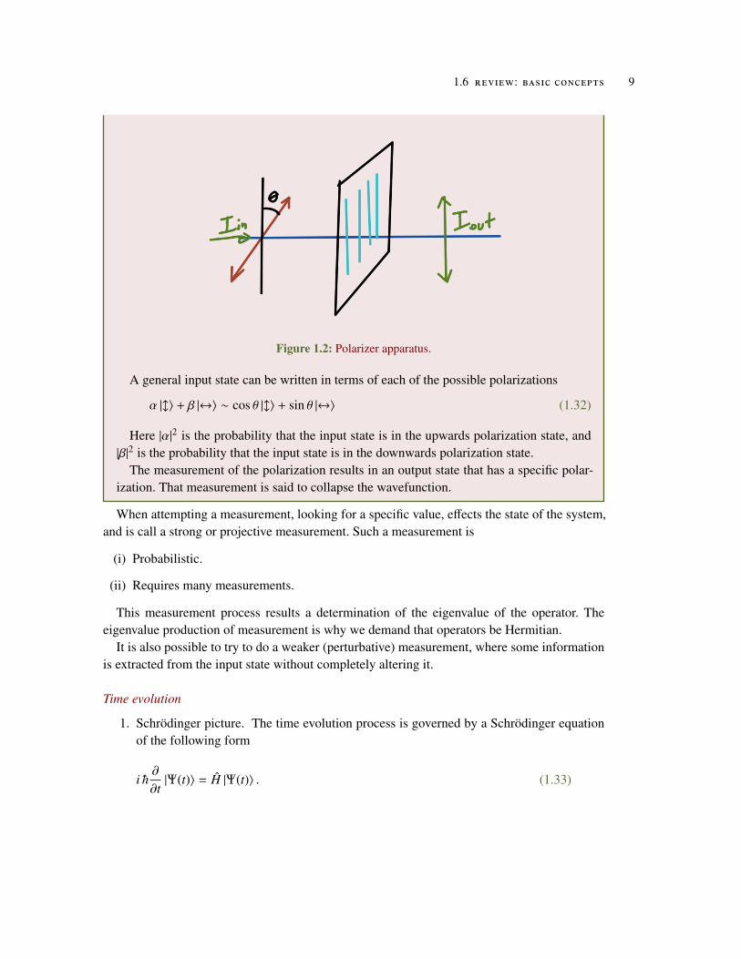
Consider a polarization apparatus as sketched in fig. 1.2, where the output is of the formIout = Iin cos2 θ.
1.6 review: basic concepts 9
Figure 1.2: Polarizer apparatus.
A general input state can be written in terms of each of the possible polarizations
(1.32)α |l〉 + β |↔〉 ∼ cos θ |l〉 + sin θ |↔〉
Here |α|2 is the probability that the input state is in the upwards polarization state, and|β|2 is the probability that the input state is in the downwards polarization state.
The measurement of the polarization results in an output state that has a specific polar-ization. That measurement is said to collapse the wavefunction.
When attempting a measurement, looking for a specific value, effects the state of the system,and is call a strong or projective measurement. Such a measurement is
(i) Probabilistic.
(ii) Requires many measurements.
This measurement process results a determination of the eigenvalue of the operator. Theeigenvalue production of measurement is why we demand that operators be Hermitian.
It is also possible to try to do a weaker (perturbative) measurement, where some informationis extracted from the input state without completely altering it.
Time evolution
1. Schrödinger picture. The time evolution process is governed by a Schrödinger equationof the following form
(1.33)i h∂
∂t|Ψ(t)〉 = H |Ψ(t)〉 .
10 fundamental concepts
This Hamiltonian could be, for example,
(1.34)H =p2
2m+ V(x),
Such a representation of time evolution is expressed in terms of operators x, p, H, · · · thatare independent of time.
2. Heisenberg picture.
Suppose we have a state |Ψ(t)〉 and operate on this with an operator
(1.35)A |Ψ(t)〉 .
This will have time evolution of the form
(1.36)Ae−iHt/ h |Ψ(0)〉 ,
or in matrix element form
(1.37)〈φ(t)| A |Ψ(t)〉 = 〈φ(0)| eiHt/ hAe−iHt/ h |Ψ(0)〉 .
We work with states that do not evolve in time |φ(0)〉 , |Ψ(0)〉 , · · ·, but operators do evolvein time according to
(1.38)A(t) = eiHt/ hAe−iHt/ h.
Density operator We can have situations where it is impossible to determine a single statethat describes the system. For example, given the gas in the room that you are sitting in, thereare things that we can measure, but it is impossible to describe the state that describes all theparticles and also impossible to construct a Hamiltonian that governs all the interactions ofthose many many particles.
We need a probabilistic description to even describe such a complex system, and to be ableto deal with concepts like entanglement.
Suppose we have a complex system that can be partitioned into two subsets, left and right, assketched in fig. 1.3.
If the states in each partition can be enumerated separately, we can write the state of thesystem as sums over the probability amplitudes that for the combined states.

1.6 review: basic concepts 11
Figure 1.3: System partitioned into separate set of states.
(1.39)|Ψ〉 =∑m,n
Cm,n |m〉 |n〉
Here Cm,n is the probability amplitude to find the state in the combined state |m〉 |n〉.As an example of such a system, we could investigate a two particle configuration where spin
up or spin down can be separately measured for each particle.
(1.40)|ψ〉 =1√
2(|↑〉 |↓〉 + |↓〉 |↑〉)
Considering such a system we could ask questions such as
• What is the probability that the left half is in state m? This would be
(1.41)∑
n
∣∣∣Cm,n∣∣∣2
• Probability that the left half is in state m, and the probability that the right half is in staten? That is
(1.42)∣∣∣Cm,n
∣∣∣2We define the density operator
(1.43)ρ = |Ψ〉 〈Ψ| .
This is idempotent

12 fundamental concepts
(1.44)ρ2 = (|Ψ〉 〈Ψ|) (|Ψ〉 〈Ψ|)= |Ψ〉 〈Ψ|
An example of a partitioned system with four total states (two spin 1/2 particles) is sketchedin fig. 1.4.
Figure 1.4: Two spins.
An example of a partitioned system with eight total states (three spin 1/2 particles) is sketchedin fig. 1.5.
Figure 1.5: Three spins.
The density matrix
(1.45)ρ = |Ψ〉 〈Ψ|
is clearly an operator as can be seen by applying it to a state
(1.46)ρ |φ〉 = |Ψ〉 (〈Ψ|φ〉) .

1.7 average of an observable 13
The quantity in braces is just a complex number.After expanding the pure state |Ψ〉 in terms of basis states for each of the two partitions
(1.47)|Ψ〉 =∑m,n
Cm,n |m〉L |n〉R ,
With L and R implied for |m〉 , |n〉 indexed states respectively, this can be written
(1.48)|Ψ〉 =∑m,n
Cm,n |m〉 |n〉 .
The density operator is
(1.49)ρ =∑m,n
Cm,nC∗m′,n′ |m〉 |n〉∑m′,n′
⟨m′
∣∣∣ ⟨n′∣∣∣ .Suppose we trace over the right partition of the state space, defining such a trace as the
reduced density operator ρred
(1.50)
ρred ≡ trR(ρ)=
∑n
〈n| ρ |n〉
=∑
n
〈n|
∑m,n
Cm,n |m〉 |n〉
∑
m′,n′C∗m′,n′
⟨m′
∣∣∣ ⟨n′∣∣∣ |n〉=
∑n
∑m,n
∑m′,n′
Cm,nC∗m′,n′ |m〉 δnn⟨m′
∣∣∣ δnn′
=∑
n,m,m′Cm,nC∗m′,n |m〉
⟨m′
∣∣∣Computing the matrix element of ρred, we have
(1.51)
〈m| ρred |m〉 =∑
m,m′,n
Cm,nC∗m′,n 〈m|m〉⟨m′
∣∣∣m⟩=
∑n
∣∣∣Cm,n∣∣∣2.
This is the probability that the left partition is in state m.

14 fundamental concepts
Figure 1.6: Magnetic moments from two spins.
1.7 average of an observable
Suppose we have two spin half particles. For such a system the total magnetization is
(1.52)S Total = S z1 + S z
1,
as sketched in fig. 1.6.The average of some observable is
(1.53)⟨A⟩
=∑
m,n,m′,n′C∗m,nCm′,n′ 〈m| 〈n| A
∣∣∣n′⟩ ∣∣∣m′⟩ .Consider the trace of the density operator observable product
(1.54)tr(ρA) =∑m,n
〈mn|Ψ〉 〈Ψ| A |m, n〉 .
Let
(1.55)|Ψ〉 =∑m,n
Cmn |m, n〉 ,
so that
(1.56)
tr(ρA) =∑
m,n,m′,n′,m′′,n′′Cm′,n′C∗m′′,n′′
⟨mn
∣∣∣m′, n′⟩ ⟨m′′, n′′∣∣∣ A |m, n〉
=∑
m,n,m′′,n′′Cm,nC∗m′′,n′′
⟨m′′, n′′
∣∣∣ A |m, n〉 .
This is just
〈Ψ| A |Ψ〉 = tr(ρA). (1.57)

1.8 left observables 15
1.8 left observables
Consider
(1.58)
〈Ψ| AL |Ψ〉 = tr(ρAL)= trL trR(ρAL)= trL
((trR ρ) AL)
)= trL
(ρredAL)
).
We see
(1.59)〈Ψ| AL |Ψ〉 = trL(ρred,LAL
).
We find that we don’t need to know the state of the complete system to answer questionsabout portions of the system, but instead just need ρ, a “probability operator” that provides allthe required information about the partitioning of the system.
1.9 pure states vs . mixed states
For pure states we can assign a state vector and talk about reduced scenarios. For mixed stateswe must work with reduced density matrices.
Example 1.2: Two particle spin half pure states
Consider
(1.60)|ψ1〉 =1√
2(|↑↓〉 − |↓↑〉)
(1.61)|ψ2〉 =1√
2(|↑↓〉 + |↑↑〉) .
For the first pure state the density operator is
(1.62)ρ =12
(|↑↓〉 − |↓↑〉) (〈↑↓| − 〈↓↑|)
What are the reduced density matrices?
(1.63)ρL = trR (ρ)
=12
(−1)(−1) |↓〉 〈↓| +12
(+1)(+1) |↑〉 〈↑| ,

16 fundamental concepts
so the matrix representation of this reduced density operator is
(1.64)ρL =12
1 0
0 1
.For the second pure state the density operator is
(1.65)ρ =12
(|↑↓〉 + |↑↑〉) (〈↑↓| + 〈↑↑|) .
This has a reduced density matrix
(1.66)
ρL = trR (ρ)
=12|↑〉 〈↑| +
12|↑〉 〈↑|
= |↑〉 〈↑| .
This has a matrix representation
(1.67)ρL =
1 0
0 0
.In this second example, we have more information about the left partition. That will be
seen as a zero entanglement entropy in the problem set. In contrast we have less informa-tion about the first state, and will find a non-zero positive entanglement entropy in thatcase.
1.10 entropy when density operator has zero eigenvalues
In the class notes and the text [11] the Von Neumann entropy is defined as
(1.68)S = − tr(ρ ln ρ).
In one of our problems I had trouble evaluating this, having calculated a density operatormatrix representation
(1.69)ρ = E ∧ E−1,
where
(1.70)E =1√
2
1 1
1 −1
,

1.10 entropy when density operator has zero eigenvalues 17
and
(1.71)∧ =
1 0
0 0
.The usual method of evaluating a function of a matrix is to assume the function has a power
series representation, and that a similarity transformation of the form A = E ∧ E−1 is possible,so that
(1.72)f (A) = E f (∧)E−1,
however, when attempting to do this with the matrix of eq. (1.69) leads to an undesirableresult
(1.73)ln ρ =12
1 1
1 −1
ln 1 0
0 ln 0
1 1
1 −1
.The ln 0 makes the evaluation of this matrix logarithm rather unpleasant. To give meaning to
the entropy expression, we have to do two things, the first is treating the trace operation as ahigher precedence than the logarithms that it contains. That is
(1.74)
− tr(ρ ln ρ) = − tr(E ∧ E−1E ln∧E−1)= − tr(E ∧ ln∧E−1)= − tr(E−1E ∧ ln∧)= − tr(∧ ln∧)= −
∑k
∧kk ln∧kk.
Now the matrix of the logarithm need not be evaluated, but we still need to give meaning to∧kk ln∧kk for zero diagonal entries. This can be done by considering a limiting scenario
(1.75)− lim
a→0a ln a = − lim
x→∞e−x ln e−x
= limx→∞
xe−x
= 0.
The entropy can now be expressed in the unambiguous form, summing over all the non-zeroeigenvalues of the density operator
S = −∑∧kk,0
∧kk ln∧kk. (1.76)

18 fundamental concepts
1.11 problems
Exercise 1.1 Representation of 2 × 2 matrix with Pauli matrices. ([11] pr. 1.2)Given an arbitrary 2×2 matrix X = a0 +σ ·a, show the relationships between aµ and tr (X), tr (σkX),and Xi j.Answer for Exercise 1.1
Observe that each of the Pauli matrices σk are traceless
σx =
0 1
1 0
σy =
0 −i
i 0
σz =
1 0
0 −1
, (1.77)
so tr (X) = 2a0. Note that tr (σkσm) = 2δkm, so tr (σkX) = 2ak.Notationally, it would seem to make sense to define σ0 ≡ I, so that tr (σµX) = aµ. I don’t
know if that is common practice.For the opposite relations, given
(1.78)
X = a0 + σ · a
=
1 0
0 1
a0 +
0 1
1 0
a1 +
0 −i
i 0
a2 +
1 0
0 −1
a3
=
a0 + a3 a1 − ia2
a1 + ia2 a0 − a3
=
X11 X12
X21 X22
,so
a0 =12(X11 + X22)
a1 =12(X12 + X21)
a2 =12i
(X21 − X12)
a3 =12(X11 − X22)
. (1.79)

1.11 problems 19
Exercise 1.2 Rotation transformation. ([11] pr. 1.3)
Determine the structure and determinant of the transformation
σ · a→ σ · a′ = exp (iσ · nφ/2)σ · a exp (−iσ · nφ/2) . (1.80)
Answer for Exercise 1.2Knowing Geometric Algebra, this is recognized as a rotation transformation. In GA, i is
treated as a pseudoscalar (which commutes with all grades in R3), and the expression can bereduced to one involving dot and wedge products. Let’s see how can this be reduced using onlythe Pauli matrix toolbox.
First, consider the determinant of one of the exponentials. Showing that one such exponentialhas unit determinant is sufficient. The matrix representation of the unit normal is
(1.81)
σ · n = nx
0 1
1 0
+ ny
0 −i
i 0
+ nz
1 0
0 −1
=
nz nx − iny
nx + iny −nz
.This is expected to have a unit square, and does
(1.82)
(σ · n)2 =
nz nx − iny
nx + iny −nz
nz nx − iny
nx + iny −nz
=
(n2
x + n2y + n2
z
) 1 0
0 1
= 1.
This allows for a cosine and sine expansion of the exponential, as in
(1.83)
exp (iσ · nθ) = cos θ + iσ · n sin θ
= cos θ
1 0
0 1
+ i sin θ
nz nx − iny
nx + iny −nz
=
cos θ + inz sin θ (nx − iny) i sin θ
(nx + iny) i sin θ cos θ − inz sin θ
.This has determinant
20 fundamental concepts
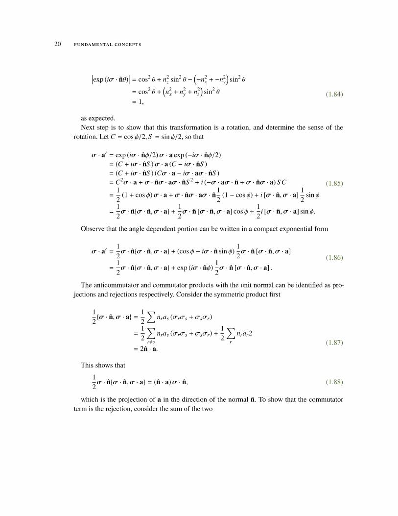
(1.84)
∣∣∣exp (iσ · nθ)∣∣∣ = cos2 θ + n2
z sin2 θ −(−n2
x + −n2y
)sin2 θ
= cos2 θ +(n2
x + n2y + n2
z
)sin2 θ
= 1,
as expected.Next step is to show that this transformation is a rotation, and determine the sense of the
rotation. Let C = cos φ/2, S = sin φ/2, so that
(1.85)
σ · a′ = exp (iσ · nφ/2)σ · a exp (−iσ · nφ/2)= (C + iσ · nS )σ · a (C − iσ · nS )= (C + iσ · nS ) (Cσ · a − iσ · aσ · nS )= C2σ · a + σ · nσ · aσ · nS 2 + i (−σ · aσ · n + σ · nσ · a) S C
=12
(1 + cos φ)σ · a + σ · nσ · aσ · n12
(1 − cos φ) + i [σ · n,σ · a]12
sin φ
=12σ · nσ · n,σ · a +
12σ · n [σ · n,σ · a] cos φ +
12
i [σ · n,σ · a] sin φ.
Observe that the angle dependent portion can be written in a compact exponential form
(1.86)σ · a′ =
12σ · nσ · n,σ · a + (cos φ + iσ · n sin φ)
12σ · n [σ · n,σ · a]
=12σ · nσ · n,σ · a + exp (iσ · nφ)
12σ · n [σ · n,σ · a] .
The anticommutator and commutator products with the unit normal can be identified as pro-jections and rejections respectively. Consider the symmetric product first
(1.87)
12σ · n,σ · a =
12
∑nras (σrσs + σsσr)
=12
∑r,s
nras (σrσs + σsσr) +12
∑r
nrar2
= 2n · a.
This shows that
(1.88)12σ · nσ · n,σ · a = (n · a)σ · n,
which is the projection of a in the direction of the normal n. To show that the commutatorterm is the rejection, consider the sum of the two

1.11 problems 21
(1.89)12σ · nσ · n,σ · a +
12σ · n [σ · n,σ · a] = σ · nσ · nσ · a
= σ · a,
so we must have
(1.90)σ · a − (n · a)σ · n =12σ · n [σ · n,σ · a] .
This is the component of a that has the projection in the n direction removed. Looking backto eq. (1.86), the transformation leaves components of the vector that are colinear with the unitnormal unchanged, and applies an exponential operation to the component that lies in whatis presumed to be the rotation plane. To verify that this latter portion of the transformationis a rotation, and to determine the sense of the rotation, let’s expand the factor of the sine ofeq. (1.85).
That is
(1.91)
i2
[σ · n,σ · a] =i2
∑nras [σr, σs]
=i2
∑nras2iεrstσt
= −∑
σtnrasεrst
= −σ · (n × a)= σ · (a × n) .
Since a × n = (a − n(n · a)) × n, this vector is seen to lie in the plane normal to n, butperpendicular to the rejection of n from a. That completes the demonstration that this is arotation transformation.
To understand the sense of this rotation, consider n = z, a = x, so
(1.92)σ · (a × n) = σ · (x × z)= −σ · y,
and
(1.93)σ · a′ = x cos φ − y sin φ,
showing that this rotation transformation has a clockwise sense.
Exercise 1.3 Some bra-ket manipulation problems. ([11] pr. 1.4)
Using braket logic expand

22 fundamental concepts
a.
tr XY (1.94)
b.
(XY)† (1.95)
c.
ei f (A), (1.96)
where A is Hermitian with a complete set of eigenvalues.
d. ∑a′
Ψa′(x′)∗Ψa′(x′′), (1.97)
where Ψa′(x′′) = 〈x′|a′〉.
Answer for Exercise 1.3
Part a.
(1.98)
tr XY =∑
a
〈a| XY |a〉
=∑a,b
〈a| X |b〉 〈b|Y |a〉
=∑a,b
〈b|Y |a〉 〈a| X |b〉
=∑a,b
〈b|YX |b〉
= tr YX.

1.11 problems 23
Part b.
(1.99)
〈a| (XY)† |b〉 = (〈b| XY |a〉)∗
=∑
c
(〈b| X |c〉 〈c|Y |a〉)∗
=∑
c
(〈b| X |c〉)∗ (〈c|Y |a〉)∗
=∑
c
(〈c|Y |a〉)∗ (〈b| X |c〉)∗
=∑
c
〈a|Y† |c〉 〈c| X† |b〉
= 〈a|Y†X† |b〉 ,
so (XY)† = Y†X†.
Part c. Let’s presume that the function f has a Taylor series representation
(1.100)f (A) =∑
r
brAr.
If the eigenvalues of A are given by
(1.101)A |as〉 = as |as〉 ,
this operator can be expanded like
(1.102)
A =∑as
A |as〉 〈as|
=∑as
as |as〉 〈as| ,
To compute powers of this operator, consider first the square
(1.103)
A2 =
=∑as
as |as〉 〈as|∑ar
ar |ar〉 〈ar |
=∑as,ar
asar |as〉 〈as| |ar〉 〈ar |
=∑as,ar
asar |as〉 δsr 〈ar |
=∑as
a2s |as〉 〈as| .

24 fundamental concepts
The pattern for higher powers will clearly just be
(1.104)Ak =∑as
aks |as〉 〈as| ,
so the expansion of f (A) will be
(1.105)
f (A) =∑
r
brAr
=∑
r
br
∑as
ars |as〉 〈as|
=∑as
∑r
brars
|as〉 〈as|
=∑as
f (as) |as〉 〈as| .
The exponential expansion is
(1.106)
ei f (A) =∑
t
it
t!f t(A)
=∑
t
it
t!
∑as
f (as) |as〉 〈as|
t
=∑
t
it
t!
∑as
f t(as) |as〉 〈as|
=∑as
ei f (as) |as〉 〈as| .
Part d.
(1.107)
∑a′
Ψa′(x′)∗Ψa′(x′′) =∑a′
⟨x′
∣∣∣a′⟩∗ ⟨x′′∣∣∣a′⟩=
∑a′
⟨a′
∣∣∣x′⟩ ⟨x′′∣∣∣a′⟩=
∑a′
⟨x′′
∣∣∣a′⟩ ⟨a′∣∣∣x′⟩=
⟨x′′
∣∣∣x′⟩= δ
(x′′ − x′
).
Exercise 1.4 Operator matrix representation. ([11] pr. 1.5)

1.11 problems 25
a. Determine the matrix representation of |α〉 〈β| given a complete set of eigenvectors |ar〉.
b. Verify with |α〉 = |sz = h/2〉 , |sx = h/2〉.
Answer for Exercise 1.4
Part a. Forming the matrix element
(1.108)⟨ar
∣∣∣ (|α〉 〈β|) ∣∣∣as⟩ =⟨ar
∣∣∣α⟩ ⟨β∣∣∣as⟩=
⟨ar
∣∣∣α⟩ ⟨as∣∣∣β⟩∗ ,
the matrix representation is seen to be
(1.109)
|α〉 〈β| ∼
⟨a1
∣∣∣ (|α〉 〈β|) ∣∣∣a1⟩ ⟨
a1∣∣∣ (|α〉 〈β|) ∣∣∣a2
⟩· · ·⟨
a2∣∣∣ (|α〉 〈β|) ∣∣∣a1
⟩ ⟨a2
∣∣∣ (|α〉 〈β|) ∣∣∣a2⟩· · ·
......
. . .
=
⟨a1
∣∣∣α⟩ ⟨a1
∣∣∣β⟩∗ ⟨a1
∣∣∣α⟩ ⟨a2
∣∣∣β⟩∗ · · ·⟨a2
∣∣∣α⟩ ⟨a1
∣∣∣β⟩∗ ⟨a2
∣∣∣α⟩ ⟨a2
∣∣∣β⟩∗ · · ·...
.... . .
.Part b. First compute the spin-z representation of |sx = h/2〉.
(1.110)(S x − h/2I)
ab =
0 h/2
h/2 0
− h/2 0
0 h/2
=
ab =
h2
−1 1
1 −1
ab
,so |sx = h/2〉 ∝ (1, 1).Normalized we have
|α〉 = |sz = h/2〉 =
10
|β〉 = |sz = h/2〉1√
2
11 .
(1.111)
Using eq. (1.109) the matrix representation is
(1.112)
|α〉 〈β| ∼
(1)(1/√
2)∗ (1)(1/√
2)∗
(0)(1/√
2)∗ (0)(1/√
2)∗
=
1√
2
1 1
0 0
.

26 fundamental concepts
This can be confirmed with direct computation
(1.113)
|α〉 〈β| =
10 1√
2
[1 1
]=
1√
2
1 1
0 0
.Exercise 1.5 Eigenvalue of sum of kets. ([11] pr. 1.6)
Given eigenkets |i〉 , | j〉 of an operator A, what are the conditions that |i〉+ | j〉 is also an eigen-vector?Answer for Exercise 1.5
Let A |i〉 = i |i〉 , A | j〉 = j | j〉, and suppose that the sum is an eigenket. Then there must be avalue a such that
(1.114)A (|i〉 + | j〉) = a (|i〉 + | j〉) ,
so(1.115)i |i〉 + j | j〉 = a (|i〉 + | j〉) .
Operating with 〈i| , 〈 j| respectively, gives
i = a
j = a,(1.116)
so for the sum to be an eigenket, both of the corresponding energy eigenvalues must beidentical (i.e. linear combinations of degenerate eigenkets are also eigenkets).
Exercise 1.6 Null operator. ([11] pr. 1.7)Given eigenkets |a′〉 of operator A
a. show that
∏a′
(A − a′) (1.117)
is the null operator.
b. ∏a′′,a′
(A − a′′)a′ − a′′
(1.118)
c. Illustrate using S z for a spin 1/2 system.
Answer for Exercise 1.6

1.11 problems 27
Part a. Application of |a〉, the eigenket of A with eigenvalue a to any term A − a′ scales |a〉by a − a′, so the product operating on |a〉 is
∏a′
(A − a′) |a〉 =∏
a′(a − a′) |a〉 . (1.119)
Since |a〉 is one of the |a′〉 eigenkets of A, one of these terms must be zero.
Part b. Again, consider the action of the operator on |a〉,
∏a′′,a′
(A − a′′)a′ − a′′
|a〉 =∏
a′′,a′
(a − a′′)a′ − a′′
|a〉 . (1.120)
If |a〉 = |a′〉, then∏
a′′,a′(A−a′′)a′−a′′ |a〉 = |a〉, whereas if it does not, then it equals one of the a′′
energy eigenvalues. This is a representation of the Kronecker delta function
(1.121)∏
a′′,a′
(A − a′′)a′ − a′′
|a〉 ≡ δa′,a |a〉
Part c. For operator S z the eigenvalues are h/2,− h/2, so the null operator must be
(1.122)
∏a′
(A − a′
)=
(h2
)21 0
0 −1
−1 0
0 1
1 0
0 −1
+
1 0
0 1
=
0 0
0 −2
2 0
0 0
=
0 0
0 0
For the delta representation, consider the |±〉 states and their eigenvalue. The delta operators
are∏a′′, h/2
(A − a′′)h/2 − a′′
=S z − (− h/2)Ih/2 − (− h/2)
=12
(σz + I) =12
1 0
0 −1
+
1 0
0 1
=
12
2 0
0 0
=
1 0
0 0
.(1.123)
∏a′′,− h/2
(A − a′′)− h/2 − a′′
=S z − ( h/2)I− h/2 − h/2
=12
(σz − I) =12
1 0
0 −1
−1 0
0 1
=
12
0 0
0 −2
=
0 0
0 1
.(1.124)

28 fundamental concepts
These clearly have the expected delta function property acting on kets |+〉 = (1, 0)T, |−〉 =
(0, 1)T.
Exercise 1.7 Spin half general normal. ([11] pr. 1.9)
Construct |S · n; +〉, where n = (cosα sin β, sinα sin β, cos β)T such that
(1.125)S · n |S · n; +〉 =h2|S · n; +〉 ,
Solve this as an eigenvalue problem.Answer for Exercise 1.7
The spin operator for this direction is
(1.126)
S · n =h2σ · n
=h2
cosα sin β
0 1
1 0
+ sinα sin β
0 −i
i 0
+ cos β
1 0
0 −1
=h2
cos β e−iα sin β
eiα sin β − cos β
.Observed that this is traceless and has a − h/2 determinant like any of the x, y, z spin opera-
tors.Assuming that this has an h/2 eigenvalue (to be verified later), the eigenvalue problem is
(1.127)
0 = S · n − h/2I
=h2
cos β − 1 e−iα sin β
eiα sin β − cos β − 1
= h
− sin2 β2 e−iα sin β
2 cos β2
eiα sin β2 cos β
2 − cos2 β2
This has a zero determinant as expected, and the eigenvector (a, b) will satisfy
(1.128)0 = − sin2 β
2a + e−iα sin
β
2cos
β
2b
= sinβ
2
(− sin
β
2a + e−iαb cos
β
2
)
(1.129)
ab ∝
cos β2
eiα sin β2
.

1.11 problems 29
This is appropriately normalized, so the ket for S · n is
(1.130)|S · n; +〉 = cosβ
2|+〉 + eiα sin
β
2|−〉 .
Note that the other eigenvalue is
(1.131)|S · n;−〉 = − sinβ
2|+〉 + eiα cos
β
2|−〉 .
It is straightforward to show that these are orthogonal and that this has the − h/2 eigenvalue.
Exercise 1.8 Two state Hamiltonian. ([11] pr. 1.10)
Solve the eigenproblem for
(1.132)H = a(|1〉 〈1| − |2〉 〈2| + |1〉 〈2| + |2〉 〈1|)
Answer for Exercise 1.8In matrix form the Hamiltonian is
(1.133)H = a
1 1
1 −1
.The eigenvalue problem is
(1.134)
0 = |H − λI|= (a − λ)(−a − λ) − a2
= (−a + λ)(a + λ) − a2
= λ2 − a2 − a2,
or
(1.135)λ = ±√
2a.
An eigenket proportional to (α, β) must satisfy
(1.136)0 = (1 ∓√
2)α + β,
so
(1.137)|±〉 ∝
−1
1 ∓√
2
,or

30 fundamental concepts
(1.138)
|±〉 =1
2(2 −√
2)
−1
1 ∓√
2
=
2 +√
24
−1
1 ∓√
2
.That is
(1.139)|±〉 =2 +√
24
(− |1〉 + (1 ∓
√2) |2〉
).
Exercise 1.9 Spin half probability and dispersion. ([11] pr. 1.12, phy1520 2015 ps1.3)A spin 1/2 system S · n, with n = sin θx + cos θz, is in state with eigenvalue h/2.
a. If S x is measured. What is the probability of getting + h/2?
b. Evaluate the dispersion in S x, that is,
⟨(S x − 〈S x〉)
2⟩. (1.140)
Answer for Exercise 1.9
Part a. In matrix form the spin operator for the system is
(1.141)
S · n =h2
cos θ
1 0
0 −1
+ sin θ
0 1
1 0
=h2
cos θ sin θ
sin θ − cos θ
An eigenket |S · n; +〉 = (a, b)T must satisfy
(1.142)
0 = (cos θ − 1) a + sin θb
=
(−2 sin2 θ
2
)a + 2 sin
θ
2cos
θ
2b
= − sinθ
2a + cos
θ
2b,
so the eigenstate is
(1.143)|S · n; +〉 =
cos θ2
sin θ2
.

1.11 problems 31
Pick |S x;±〉 = 1√2
1
±1
as the basis for the S x operator. Then, for the probability that the
system will end up in the + h/2 state of S x, we have
(1.144)
P = |〈S x; +|S · n; +〉|2
=
∣∣∣∣∣∣∣∣ 1√
2
11† cos θ
2
sin θ2
∣∣∣∣∣∣∣∣2
=12
∣∣∣∣∣∣∣[1 1] cos θ
2
sin θ2
∣∣∣∣∣∣∣2
=12
(cos
θ
2+ sin
θ
2
)2
=12
(1 + 2 cos
θ
2sin
θ
2
)=
12
(1 + sin θ) .
This is a reasonable seeming result, with P ∈ [0, 1]. Some special values also further validatethis
θ = 0, |S · n; +〉 =
10 = |S z; +〉 =
1√
2|S x; +〉 +
1√
2|S x;−〉
θ = π/2, |S · n; +〉 =1√
2
11 = |S x; +〉
θ = π, |S · n; +〉 =
01 = |S z;−〉 =
1√
2|S x; +〉 −
1√
2|S x;−〉 ,
(1.145)
where we see that the probabilities are in proportion to the projection of the initial state ontothe measured state |S x; +〉.
Part b. The S x expectation is
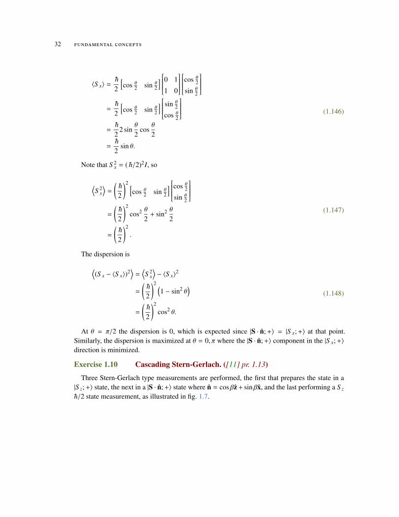
32 fundamental concepts
(1.146)
〈S x〉 =h2
[cos θ
2 sin θ2
] 0 1
1 0
cos θ
2
sin θ2
=
h2
[cos θ
2 sin θ2
] sin θ2
cos θ2
=
h2
2 sinθ
2cos
θ
2
=h2
sin θ.
Note that S 2x = ( h/2)2I, so
(1.147)
⟨S 2
x
⟩=
(h2
)2 [cos θ
2 sin θ2
] cos θ2
sin θ2
=
(h2
)2
cos2 θ
2+ sin2 θ
2
=
(h2
)2
.
The dispersion is
(1.148)
⟨(S x − 〈S x〉)2
⟩=
⟨S 2
x
⟩− 〈S x〉
2
=
(h2
)2 (1 − sin2 θ
)=
(h2
)2
cos2 θ.
At θ = π/2 the dispersion is 0, which is expected since |S · n; +〉 = |S x; +〉 at that point.Similarly, the dispersion is maximized at θ = 0, π where the |S · n; +〉 component in the |S x; +〉
direction is minimized.
Exercise 1.10 Cascading Stern-Gerlach. ([11] pr. 1.13)
Three Stern-Gerlach type measurements are performed, the first that prepares the state in a|S z; +〉 state, the next in a |S · n; +〉 state where n = cos βz + sin βx, and the last performing a S z
h/2 state measurement, as illustrated in fig. 1.7.

1.11 problems 33
Figure 1.7: Cascaded Stern-Gerlach type measurements.
What is the intensity of the final sz = − h/2 beam? What is the orientation for the secondmeasuring apparatus to maximize the intensity of this beam?Answer for Exercise 1.10
The spin operator for the second apparatus is
(1.149)
S · n =h2
sin β
0 1
1 0
+ cos β
1 0
0 −1
=h2
cos β sin β
sin β − cos β
.The intensity of the final |S z;−〉 beam is
(1.150)P = |〈−|S · n; +〉 〈S · n; +|+〉|2,
(i.e. the second apparatus applies a projection operator |S · n; +〉 〈S · n; +| to the initial |+〉state, and then the |−〉 states are selected out of that.
The S · n eigenket is found to be
(1.151)|S · n; +〉 =
cos β2
sin β2
,so

34 fundamental concepts
(1.152)
P =
∣∣∣∣∣∣∣[0 1] cos β
2
sin β2
[cos β2 sin β
2
] 10∣∣∣∣∣∣∣2
=
∣∣∣∣∣cosβ
2sin
β
2
∣∣∣∣∣2=
∣∣∣∣∣12 sin β∣∣∣∣∣2
=14
sin2 β.
This is maximized when β = π/2, or n = x. At this angle the state leaving the secondapparatus is
(1.153)
cos β2
sin β2
[cos β2 sin β
2
] 10 =
12
11 [1 1
] 10
=12
11
=12|+〉 +
12|−〉 ,
so the state after filtering the |−〉 states is 12 |−〉 with intensity (probability density) of 1/4
relative to a unit normalize input |+〉 state to the S · n apparatus.
Exercise 1.11 Can anticommuting operators have a simultaneous eigenket? ([11] pr. 1.16)
Two Hermitian operators anticommute
(1.154)A, B = AB + BA= 0.
Is it possible to have a simultaneous eigenket of A and B? Prove or illustrate your assertion.Answer for Exercise 1.11
Suppose that such a simultaneous non-zero eigenket |α〉 exists, then
(1.155)A |α〉 = a |α〉 ,
and
(1.156)B |α〉 = b |α〉
This gives

1.11 problems 35
(1.157)(AB + BA) |α〉 = (Ab + Ba) |α〉= 2ab |α〉 .
If this is zero, one of the operators must have a zero eigenvalue. Knowing that we can con-struct an example of such operators. In matrix form, let
(1.158a)A =
1 0 0
0 −1 0
0 0 a
(1.158b)B =
0 1 0
1 0 0
0 0 b
.These are both Hermitian, and anticommute provided at least one of a, b is zero. These have
a common eigenket
(1.159)|α〉 =
0
0
1
.A zero eigenvalue of one of the commuting operators may not be a sufficient condition for
such anticommutation.
Exercise 1.12 Degeneracy in non-commuting observables that both commute with the Hamiltonian. ([11] pr. 1.17)
Show that non-commuting operators that both commute with the Hamiltonian, have, in gen-eral, degenerate energy eigenvalues. That is
[A,H] = [B,H] = 0, (1.160)
but
(1.161)[A, B] , 0.
a. Consider Lx, Lz and a central force Hamiltonian H = p2/2m + V(r) as examples.
b. Construct some simple matrix examples that illustrate the degeneracy conditions.
c. Prove the general case.
Answer for Exercise 1.12

36 fundamental concepts
Part a. Let’s start with demonstrate these commutators act as expected in these cases.With L = x × p, we have
Lx = ypz − zpy
Ly = zpx − xpz
Lz = xpy − ypx.
(1.162)
The Lx, Lz commutator is
[Lx, Lz] = [ypz − zpy, xpy − ypx]
= [ypz, xpy] − [ypz, ypx] − [zpy, xpy] + [zpy, ypx]
= xpz [y, py] + zpx [py, y]
= i h (xpz − zpx)
= −i hLy
(1.163)
cyclically permuting the indexes shows that no pairs of different L components commute. ForLy, Lx that is
[Ly, Lx] = [zpx − xpz, ypz − zpy]
= [zpx, ypz] − [zpx, zpy] − [xpz, ypz] + [xpz, zpy]
= ypx [z, pz] + xpy [pz, z]
= i h (ypx − xpy)
= −i hLz,
(1.164)
and for Lz, Ly
[Lz, Ly] = [xpy − ypx, zpx − xpz]
= [xpy, zpx] − [xpy, xpz] − [ypx, zpx] + [ypx, xpz]
= zpy [x, px] + ypz [px, x]
= i h (zpy − ypz)
= −i hLx.
(1.165)
If these angular momentum components are also shown to commute with themselves (whichthey do), the commutator relations above can be summarized as
[La, Lb] = i hεabcLc. (1.166)

1.11 problems 37
In the example to consider, we’ll have to consider the commutators with p2 and V(r). Pickingany one component of L is sufficient due to the symmetries of the problem. For example
[Lx,p2
]=
[ypz − zpy, p2
x + p2y + p2
z
]=
[ypz,p
2x + p2
y +p2z
]−
[zpy,p
2x +p2y + p2
z
]= pz
[y, p2
y
]− py
[z, p2
z
]= pz2i hpy − py2i hpz
= 0.
(1.167)
How about the commutator of L with the potential? It is sufficient to consider one componentagain, for example
[Lx,V ] = [ypz − zpy,V ]
= y [pz,V ] − z [py,V ]
= −i hy∂V(r)∂z
+ i hz∂V(r)∂y
= −i hy∂V∂r
∂r∂z
+ i hz∂V∂r
∂r∂y
= −i hy∂V∂r
zr
+ i hz∂V∂r
yr
= 0.
(1.168)
This has shown that all the components of L commute with a central force Hamiltonian, andeach different component of L do not commute. It does not demonstrate the degeneracy, but Ido recall that exists for this system.

38 fundamental concepts
Part b. I thought perhaps the problem at hand would be easier if I were to construct someexample matrices representing operators that did not commute, but did commuted with a Hamil-tonian. I came up with
A =
σz 0
0 1
=
1 0 0
0 −1 0
0 0 1
B =
σx 0
0 1
=
0 1 0
1 0 0
0 0 1
H =
0 0 0
0 0 0
0 0 1
(1.169)
This system has [A,H] = [B,H] = 0, and
(1.170)[A, B] =
0 2 0
−2 0 0
0 0 0
There is one shared eigenvector between all of A, B,H
(1.171)|3〉 =
0
0
1
.The other eigenvectors for A are
|a1〉 =
1
0
0
|a2〉 =
0
1
0
,(1.172)

1.11 problems 39
and for B
|b1〉 =1√
2
1
1
0
|b2〉 =
1√
2
1
−1
0
,(1.173)
This clearly has the degeneracy sought.Looking to [1], it appears that it is possible to construct an even simpler example. Let
A =
0 1
0 0
B =
1 0
0 0
H =
0 0
0 0
.(1.174)
Here [A, B] = −A, and [A,H] = [B,H] = 0, but the Hamiltonian isn’t interesting at allphysically.
A less boring example builds on this. Let
A =
0 1 0
0 0 0
0 0 1
B =
1 0 0
0 0 0
0 0 1
H =
0 0 0
0 0 0
0 0 1
.
(1.175)
Here [A, B] , 0, and [A,H] = [B,H] = 0. I don’t see a way for any exception to be con-structed.

40 fundamental concepts
Part c. The concrete examples above give some intuition for solving the more abstract prob-lem. Suppose that we are working in a basis that simultaneously diagonalizes operator A andthe Hamiltonian H. To make life easy consider the simplest case where this basis is also aneigenbasis for the second operator B for all but two of that operators eigenvectors. For such asystem let’s write
H |1〉 = ε1 |1〉
H |2〉 = ε2 |2〉
A |1〉 = a1 |1〉
A |2〉 = a2 |2〉 ,
(1.176)
where |1〉, and |2〉 are not eigenkets of B. Because B also commutes with H, we must have
(1.177)HB |1〉 = H |n〉 〈n| B |1〉= εn |n〉 Bn1,
and
(1.178)BH |1〉 = Bε1 |1〉
= ε1 |n〉 〈n| B |1〉= ε1 |n〉 Bn1.
The commutator is
(1.179)[B,H] |1〉 = (ε1 − εn) |n〉 Bn1.
Similarly
(1.180)[B,H] |2〉 = (ε2 − εn) |n〉 Bn2.
For those kets |m〉 ∈ |3〉 , |4〉 , · · · that are eigenkets of B, with B |m〉 = bm |m〉, we have
(1.181)[B,H] |m〉 = Bεm |m〉 − Hbm |m〉
= bmεm |m〉 − εmbm |m〉= 0.
If the commutator is zero, then we require all its matrix elements
〈1| [B,H] |1〉 = (ε1 − ε1) B11
〈2| [B,H] |1〉 = (ε1 − ε2) B21
〈1| [B,H] |2〉 = (ε2 − ε1) B12
〈2| [B,H] |2〉 = (ε2 − ε2) B22,
(1.182)

1.11 problems 41
to be zero. Because of eq. (1.181) only the matrix elements with respect to states |1〉 , |2〉 needbe considered. Two of the matrix elements above are clearly zero, regardless of the values ofB11, and B22, and for the other two to be zero, we must either have
• B21 = B12 = 0, or
• ε1 = ε2.
If the first condition were true we would have
(1.183)B |1〉 = |n〉 〈n| B |1〉
= |n〉 Bn1
= |1〉 B11,
and B |2〉 = B22 |2〉. This contradicts the requirement that |1〉 , |2〉 not be eigenkets of B, leav-ing only the second option. That second option means there must be a degeneracy in the system.
Exercise 1.13 Uncertainty relation. ([11] pr. 1.20)
Find the ket that maximizes the uncertainty product
(1.184)⟨(∆S x)2
⟩ ⟨(∆S y
)2⟩,
and compare to the uncertainty bound 14
∣∣∣∣⟨[S x, S y]⟩∣∣∣∣2.
Answer for Exercise 1.13To parameterize the ket space, consider first the kets that where both components are both
not zero, where a single complex number can parameterize the ket
(1.185)
|s〉 =
β′eiφ′
α′eiθ′
∝
1
αeiθ

42 fundamental concepts
The expectation values with respect to this ket are
(1.186)
〈S x〉 =h2
[1 αe−iθ
] 0 1
1 0
1
αeiθ
=
h2
[1 αe−iθ
] αeiθ
1
=
h2αeiθ + αe−iθ
=h2
2α cos θ
= hα cos θ.
(1.187)
⟨S y
⟩=
h2
[1 αe−iθ
] 0 −i
i 0
1
αeiθ
=
i h2
[1 αe−iθ
] −αeiθ
1
=−iα h
22i sin θ
= α h sin θ.
The variances are
(1.188)
(∆S x)2 =
h2
−2α cos θ 1
1 −2α cos θ
2
=h2
4
−2α cos θ 1
1 −2α cos θ
−2α cos θ 1
1 −2α cos θ
=
h2
4
4α2 cos2 θ + 1 −4α cos θ
−4α cos θ 4α2 cos2 θ + 1
,and
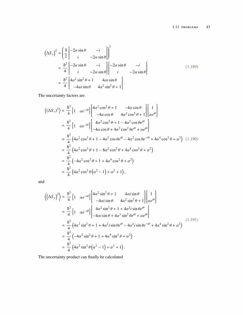
1.11 problems 43
(1.189)
(∆S y
)2=
h2
−2α sin θ −i
i −2α sin θ
2
=h2
4
−2α sin θ −i
i −2α sin θ
−2α sin θ −i
i −2α sin θ
=
h2
4
4α2 sin2 θ + 1 4αi sin θ
−4αi sin θ 4α2 sin2 θ + 1
.The uncertainty factors are
(1.190)
⟨(∆S x)2
⟩=
h2
4
[1 αe−iθ
] 4α2 cos2 θ + 1 −4α cos θ
−4α cos θ 4α2 cos2 θ + 1
1
αeiθ
=
h2
4
[1 αe−iθ
] 4α2 cos2 θ + 1 − 4α2 cos θeiθ
−4α cos θ + 4α3 cos2 θeiθ + αeiθ
=
h2
4
(4α2 cos2 θ + 1 − 4α2 cos θeiθ − 4α2 cos θe−iθ + 4α4 cos2 θ + α2
)=
h2
4
(4α2 cos2 θ + 1 − 8α2 cos2 θ + 4α4 cos2 θ + α2
)=
h2
4
(−4α2 cos2 θ + 1 + 4α4 cos2 θ + α2
)=
h2
4
(4α2 cos2 θ
(α2 − 1
)+ α2 + 1
),
and
(1.191)
⟨(∆S y
)2⟩
=h2
4
[1 αe−iθ
] 4α2 sin2 θ + 1 4αi sin θ
−4αi sin θ 4α2 sin2 θ + 1
1
αeiθ
=
h2
4
[1 αe−iθ
] 4α2 sin2 θ + 1 + 4α2i sin θeiθ
−4αi sin θ + 4α3 sin2 θeiθ + αeiθ
=
h2
4
(4α2 sin2 θ + 1 + 4α2i sin θeiθ − 4α2i sin θe−iθ + 4α4 sin2 θ + α2
)=
h2
4
(−4α2 sin2 θ + 1 + 4α4 sin2 θ + α2
)=
h2
4
(4α2 sin2 θ
(α2 − 1
)+ α2 + 1
).
The uncertainty product can finally be calculated

44 fundamental concepts
(1.192)
⟨(∆S x)2
⟩ ⟨(∆S y
)2⟩
=
(h2
)4 (4α2 cos2 θ
(α2 − 1
)+ α2 + 1
) (4α2 sin2 θ
(α2 − 1
)+ α2 + 1
)=
(h2
)4 (4α4 sin2 (2θ)
(α2 − 1
)+ 4α2
(α4 − 1
)+
(α2 + 1
)2)
The maximum occurs when f = sin2 2θ is extremized. Those points are
(1.193)0 =
∂ f∂θ
= 2 sin 2θ cos 2θ= 4 sin 4θ.
Those points are at 4θ = πn, for integer n, or
θ =π
4n, n ∈ [0, 7], (1.194)
Minimums will occur when
(1.195)0 <∂2 f∂θ2
= 8 cos 4θ,
or
(1.196)n = 0, 2, 4, 6.
At these points sin2 2θ takes the values
(1.197)sin2(2π
40, 2, 4, 6
)= sin2 (π 0, 1, 2, 3)
∈ 0 ,
so the maximization of the uncertainty product can be reduced to that of
(1.198)⟨(∆S x)2
⟩ ⟨(∆S y
)2⟩
=
(h2
)4 (4α2
(α4 − 1
)+
(α2 + 1
)2)
We seek

1.11 problems 45
(1.199)
0 =∂
∂α
(4α2
(α4 − 1
)+
(α2 + 1
)2)
=(8α
(α4 − 1
)+ 16α5 + 4
(α2 + 1
)α)
= 4α(2α4 − 2 + 4α4 + 4α2 + 4
)= 8α
(3α4 + 2α2 + 1
).
The only real root of this polynomial is α = 0, so the ket where both |+〉 and |−〉 are not zerothat maximizes the uncertainty product is
(1.200)|s〉 =
10
= |+〉 .
The search for this maximizing value excluded those kets proportional to
01 = |−〉. Let’s see
the values of this uncertainty product at both |±〉, and compare to the uncertainty commutator.First |s〉 = |+〉
(1.201)〈S x〉 =[1 0
] 0 1
1 0
10
= 0.
(1.202)⟨S y
⟩=
[1 0
] 0 −i
i 0
10
= 0.
so
(1.203)
⟨(∆S x)2
⟩=
(h2
)2 [1 0
] 10
=
(h2
)2

46 fundamental concepts
(1.204)
⟨(∆S y
)2⟩
=
(h2
)2 [1 0
] 10
=
(h2
)2
.
For the commutator side of the uncertainty relation we have
(1.205)
14
∣∣∣∣⟨[S x, S y]⟩∣∣∣∣2 =
14|〈ihS z〉|
2
=
(h2
)4∣∣∣∣∣∣∣[1 0
] 1 0
0 −1
10
∣∣∣∣∣∣∣2
,
so for the |+〉 state we have an equality condition for the uncertainty relation
(1.206)
⟨(∆S x)2
⟩ ⟨(∆S y
)2⟩
=14
∣∣∣∣⟨[S x, S y]⟩∣∣∣∣2
=
(h2
)4
.
It’s reasonable to guess that the |−〉 state also matches the equality condition. Let’s check
(1.207)〈S x〉 =[0 1
] 0 1
1 0
01
= 0.
(1.208)⟨S y
⟩=
[0 1
] 0 −i
i 0
01
= 0.
so⟨(∆S x)
2⟩=
⟨(∆S y)
2⟩=
(h2
)2.
For the commutator side of the uncertainty relation will be identical, so the equality ofeq. (1.206) is satisfied for both |±〉. Note that it wasn’t explicitly verified that |−〉maximized theuncertainty product, but I don’t feel like working through that second set of algebraic mess.
We can see by example that equality does not mean that the equality condition means thatthe product is maximized. For example, it is straightforward to show that |S x;±〉 also satisfythe equality condition of the uncertainty relation. However, in that case the product is not maxi-mized, but is zero.
1.11 problems 47
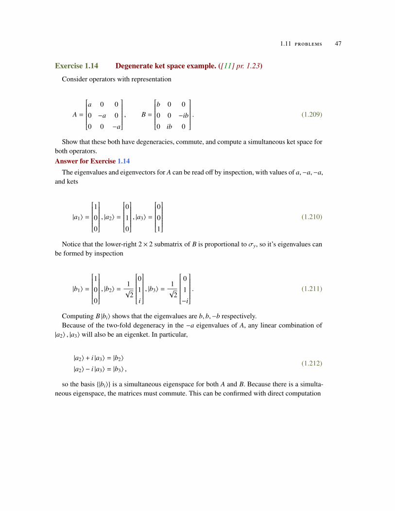
Exercise 1.14 Degenerate ket space example. ([11] pr. 1.23)
Consider operators with representation
A =
a 0 0
0 −a 0
0 0 −a
, B =
b 0 0
0 0 −ib
0 ib 0
. (1.209)
Show that these both have degeneracies, commute, and compute a simultaneous ket space forboth operators.Answer for Exercise 1.14
The eigenvalues and eigenvectors for A can be read off by inspection, with values of a,−a,−a,and kets
|a1〉 =
1
0
0
, |a2〉 =
0
1
0
, |a3〉 =
0
0
1
(1.210)
Notice that the lower-right 2 × 2 submatrix of B is proportional to σy, so it’s eigenvalues canbe formed by inspection
|b1〉 =
1
0
0
, |b2〉 =1√
2
0
1
i
, |b3〉 =1√
2
0
1
−i
. (1.211)
Computing B |bi〉 shows that the eigenvalues are b, b,−b respectively.Because of the two-fold degeneracy in the −a eigenvalues of A, any linear combination of
|a2〉 , |a3〉 will also be an eigenket. In particular,
|a2〉 + i |a3〉 = |b2〉
|a2〉 − i |a3〉 = |b3〉 ,(1.212)
so the basis |bi〉 is a simultaneous eigenspace for both A and B. Because there is a simulta-neous eigenspace, the matrices must commute. This can be confirmed with direct computation

48 fundamental concepts
(1.213)
AB = ab
1 0 0
0 −1 0
0 0 −1
1 0 0
0 0 −i
0 i 0
= ab
1 0 0
0 0 i
0 −i 0
,and
(1.214)
BA = ab
1 0 0
0 0 −i
0 i 0
1 0 0
0 −1 0
0 0 −1
= ab
1 0 0
0 0 i
0 −i 0
.
Exercise 1.15 Unitary transformation. ([11] pr. 1.26)
Construct the transformation matrix that maps between the S z diagonal basis, to the S x diag-onal basis.Answer for Exercise 1.15
Based on the definition
(1.215)U∣∣∣a(r)
⟩=
∣∣∣b(r)⟩,
the matrix elements can be computed
(1.216)⟨a(s)
∣∣∣ U ∣∣∣a(r)⟩
=⟨a(s)
∣∣∣b(r)⟩,
that is

1.11 problems 49
(1.217)
U =
⟨a(1)
∣∣∣ U ∣∣∣a(1)⟩ ⟨
a(1)∣∣∣ U ∣∣∣a(2)
⟩⟨a(2)
∣∣∣ U ∣∣∣a(1)⟩ ⟨
a(2)∣∣∣ U ∣∣∣a(2)
⟩=
⟨a(1)
∣∣∣b(1)⟩ ⟨
a(1)∣∣∣b(2)
⟩⟨a(2)
∣∣∣b(1)⟩ ⟨
a(2)∣∣∣b(2)
⟩
=1√
2
[1 0
] 11 [
1 0] 1
−1
[0 1
] 11 [
0 1] 1
−1
=
1√
2
1 1
1 −1
.As a similarity transformation, we have
(1.218)
⟨b(r)
∣∣∣ S z∣∣∣b(s)
⟩=
⟨b(r)
∣∣∣a(t)⟩ ⟨
a(t)∣∣∣ S z
∣∣∣a(u)⟩ ⟨
a(u)∣∣∣b(s)
⟩=
⟨a(r)
∣∣∣U⟩†a(t)
⟨a(t)
∣∣∣ S z∣∣∣a(u)
⟩ ⟨a(u)
∣∣∣ U ∣∣∣a(s)⟩,
or
(1.219)S ′z = U†S zU.
Let’s check that the computed similarity transformation does it’s job.
(1.220)
σ′z = U†σzU
=12
1 1
1 −1
1 0
0 −1
1 1
1 −1
=
12
1 −1
1 1
1 1
1 −1
=
12
0 2
2 0
= σx.
The transformation matrix can also be computed more directly

50 fundamental concepts
(1.221)
U = U∣∣∣a(r)
⟩ ⟨a(r)
∣∣∣=
∣∣∣b(r)⟩ ⟨
a(r)∣∣∣
=1√
2
11 [1 0
]+
1√
2
1
−1
[0 1]
=1√
2
1 0
1 0
+1√
2
0 1
0 −1
=
1√
2
1 1
1 −1
.Exercise 1.16 One dimensional translation operator. ([11] pr. 1.28)
a. Evaluate the classical Poisson bracket
(1.222)[x, F(p)
]classical
b. Evaluate the commutator
(1.223)[x, eipa/ h
]c. Using the result in b, prove that
(1.224)eipa/ h∣∣∣x′⟩ ,
is an eigenstate of the coordinate operator x.
Answer for Exercise 1.16
Part a.
(1.225)
[x, F(p)
]classical =
∂x∂x∂F(p)∂p
−∂x∂p
∂F(p)∂x
=∂F(p)∂p
.
Part b. Having worked backwards through these problems, the answer for this one dimen-sional problem can be obtained from eq. (1.246) and is
(1.226)[x, eipa/ h
]= aeipa/ h.

1.11 problems 51
Part c.
(1.227)xeipa/ h∣∣∣x′⟩ =
([x, eipa/ h
]eipa/ hx+
) ∣∣∣x′⟩ =(aeipa/ h + eipa/ hx′
) ∣∣∣x′⟩ =(a + x′
) ∣∣∣x′⟩ .This demonstrates that eipa/ h |x′〉 is an eigenstate of x with eigenvalue a + x′.
Exercise 1.17 Polynomial commutators. ([11] pr. 1.29)
a. For power series F,G, verify
[xk,G(p)] = i h∂G∂pk
, [pk, F(x)] = −i h∂F∂xk
. (1.228)
b. Evaluate[x2, p2
], and compare to the classical Poisson bracket
[x2, p2
]classical
.
Answer for Exercise 1.17
Part a. Let
G(p) =∑klm
aklm pk1 pl
2 pm3
F(x) =∑klm
bklmxk1xl
2xm3 .
(1.229)
It is simpler to work with a specific xk, say xk = y. The validity of the general result will stillbe clear doing so. Expanding the commutator gives
(1.230)
[y,G(p)
]=
∑klm
aklm[y, pk
1 pl2 pm
3
]=
∑klm
aklm(ypk
1 pl2 pm
3 − pk1 pl
2 pm3 y
)=
∑klm
aklm(pk
1ypl2 pm
3 − pk1ypl
2 pm3
)=
∑klm
aklm pk1
[y, pl
2
]pm
3 .
From eq. (1.244), we have[y, pl
2
]= li hpl−1
2 , so
(1.231)
[y,G(p)
]=
∑klm
aklm pk1
[y, pl
2
] (li hpl−1
2
)pm
3
= i h∂G(p)∂y
.

52 fundamental concepts
It is straightforward to show that[p, xl
]= −li hxl−1, allowing for a similar computation of the
momentum commutator
(1.232)
[py, F(x)
]=
∑klm
bklm[py, xk
1xl2xm
3
]=
∑klm
bklm(pyxk
1xl2xm
3 − xk1xl
2xm3 py
)=
∑klm
bklm(xk
1 pyxl2xm
3 − xk1 pyxl
2xm3
)=
∑klm
bklmxk1
[py, xl
2
]xm
3
=∑klm
bklmxk1
(−li hxl−1
2
)xm
3
= −i h∂F(x)∂py
.
Part b. It isn’t clear to me how the results above can be used directly to compute[x2, p2
].
However, when the first term of such a commutator is a mononomial, it can be expanded interms of an x commutator
(1.233)
[x2,G(p)
]= x2G −Gx2
= x (xG) −Gx2
= x ([x,G] + Gx) −Gx2
= x [x,G] + (xG) x −Gx2
= x [x,G] + ([x,G] +Gx) x −Gx2
= x [x,G] + [x,G] x.
Similarly,
(1.234)[x3,G(p)
]= x2 [x,G] + x [x,G] x + [x,G] x2.
An induction hypothesis can be formed
(1.235)[xk,G(p)
]=
k−1∑j=0
xk−1− j [x,G] x j,
and demonstrated

1.11 problems 53
(1.236)
[xk+1,G(p)
]= xk+1G −Gxk+1
= x(xkG
)−Gxk+1
= x([
xk,G]
+ Gxk)−Gxk+1
= x[xk,G
]+ (xG) xk −Gxk+1
= x[xk,G
]+ ([x,G] + Gx) xk −Gxk+1
= x[xk,G
]+ [x,G] xk
= xk−1∑j=0
xk−1− j [x,G] x j + [x,G] xk
=
k−1∑j=0
x(k+1)−1− j [x,G] x j + [x,G] xk
=
k∑j=0
x(k+1)−1− j [x,G] x j.
That was a bit overkill for this problem, but may be useful later. Application of this to theproblem gives
(1.237)
[x2, p2
]= x
[x, p2
]+
[x, p2
]x
= xi h∂p2
∂x+ i h
∂p2
∂xx
= x2i hp + 2i hpx= i h (2xp + 2px) .
The classical commutator is
(1.238)
[x2, p2
]classical
=∂x2
∂x∂p2
∂p−∂x2
∂p∂p2
∂x= 2x2p= 2xp + 2px.
This demonstrates the expected relation between the classical and quantum commutators
[x2, p2
]= i h
[x2, p2
]classical
. (1.239)

54 fundamental concepts
Exercise 1.18 Translation operator and position expectation. ([11] pr. 1.30)
The translation operator for a finite spatial displacement is given by
(1.240)T(l) = exp (−ip · l/ h) ,
where p is the momentum operator.
a. Evaluate
(1.241)[xi,T(l)] .
b. Demonstrate how the expectation value 〈x〉 changes under translation.
Answer for Exercise 1.18
Part a. For clarity, let’s set xi = y. The general result will be clear despite doing so.
(1.242)[y,T(l)
]=
∑k=0
1k!
(−ih
) [y, (p · l)k
].
The commutator expands as
(1.243)
[y, (p · l)k
]+ (p · l)k y = y (p · l)k
= y(pxlx + pyly + pzlz
)(p · l)k−1
=(pxlxy + ypyly + pzlzy
)(p · l)k−1
=(pxlxy + ly
(pyy + i h
)+ pzlzy
)(p · l)k−1
= (p · l) y (p · l)k−1 + i hly (p · l)k−1
= · · ·
= (p · l)k−1 y (p · l)k−(k−1) + (k − 1)i hly (p · l)k−1
= (p · l)k y + ki hly (p · l)k−1 .
In the above expansion, the commutation of y with px, pz has been used. This gives, for k , 0,
(1.244)[y, (p · l)k
]= ki hly (p · l)k−1 .
Note that this also holds for the k = 0 case, since y commutes with the identity operator.Plugging back into the T commutator, we have
(1.245)
[y,T(l)
]=
∑k=1
1k!
(−ih
)ki hly (p · l)k−1
= ly∑k=1
1(k − 1)!
(−ih
)(p · l)k−1
= lyT(l).

1.11 problems 55
The same pattern clearly applies with the other xi values, providing the desired relation.
[x,T(l)] =
3∑m=1
emlmT(l) = lT(l). (1.246)
Part b. Suppose that the translated state is defined as |αl〉 = T(l) |α〉. The expectation valuewith respect to this state is
(1.247)
⟨x′
⟩= 〈αl| x |αl〉
= 〈α|T†(l)xT(l) |α〉= 〈α|T†(l) (xT(l)) |α〉= 〈α|T†(l) (T(l)x + lT(l)) |α〉= 〈α|T†Tx + lT†T |α〉= 〈α| x |α〉 + l 〈α|α〉= 〈x〉 + l.
Exercise 1.19 Density matrix. (phy1520 2015 ps1.1)
Consider a spin-1/2 particle. The Hilbert space is two-dimensional, let us label the two statesas |↑〉 and |↓〉. Write down the 2 × 2 density matrix which corresponds to the following purestates.
(i) |↑〉
(ii) 1√2(|↑〉 + |↓〉)
(iii) 1√2(|↑〉 + i |↓〉)
(iv) At time t = 0, let us start with the state 1√2(|↑〉 + i |↓〉), and consider time-evolution under
the Hamiltonian H = −BS z, where S z is the z-component of the spin operator. This leadsto eigenstates |↑〉with energy −B h/2, and |↓〉with energy +B h/2. The state 1√
2(|↑〉 + i |↓〉)
is not an eigenstate of this Hamiltonian and it will evolve in time. Find the state and thecorresponding 2 × 2 density matrix of this system at a later time t.
Answer for Exercise 1.19PROBLEM SET RELATED MATERIAL REDACTED IN THIS DOCUMENT.PLEASE
FEEL FREE TO EMAIL ME FOR THE FULL VERSION IF YOU AREN’T TAKING PHY1520.. .
. .

56 fundamental concepts
.. . .
. .. . .
. .. .
. END-REDACTION
Exercise 1.20 Reduced density matrix. (phy1520 2015 ps1.2)
Consider two spin-1/2 particles, the Hilbert space is now 4-dimensional, with states |↑↑〉, |↑↓〉,|↓↑〉, |↓↓〉. Let us consider the following pure states:
(i) 12 (|↑↑〉 − |↑↓〉 − |↓↓〉 + |↓↑〉)
(ii) 1√2(|↑↑〉 + |↓↓〉)
(iii) 1√5(|↑↑〉 + 2 |↓↓〉)
In each case, obtain the reduced 2 × 2 density matrix which describes the first spin, whenwe trace over the second spin. The von Neumann entanglement entropy is defined via S vN =
− tr(ρR ln ρR) where ρR is the reduced density matrix you have obtained above and the tr nowrefers to tracing over the first spin. Using the reduced density matrices you have obtained above,compute the corresponding S vN, and simply explain your result in words. Consider the Renyientropy S n = 1
1−n ln(tr(ρn
R)). Prove that S n→1 = S vN, and compute S n=2 for the above ρR.
Answer for Exercise 1.20PROBLEM SET RELATED MATERIAL REDACTED IN THIS DOCUMENT.PLEASE
FEEL FREE TO EMAIL ME FOR THE FULL VERSION IF YOU AREN’T TAKING PHY1520.. .
. ..
. . .. .
. . .. .
. .. END-REDACTION
Exercise 1.21 Ensembles for spin one half. ([11] pr. 3.10)

1.11 problems 57
a. Sakurai leaves it to the reader to verify that knowledge of the three ensemble averages[S_x], [S_y],[S_z] is sufficient to reconstruct the density operator for a spin one halfsystem. Show this.
b. Show how the expectation values 〈S x〉 ,⟨S y
⟩, 〈S x〉 fully determine the spin orientation
for a pure ensemble.
Answer for Exercise 1.21
Part a. I’ll do this in two parts, the first using a spin-up/down ensemble to see what form thishas, then the general case. The general case is a bit messy algebraically. After first attempting itthe hard way, I did the grunt work portion of that calculation in Mathematica, but then realizedit’s not so bad to do it manually.
Consider first an ensemble with density operator
(1.248)ρ = w+ |+〉 〈+| + w− |−〉 〈−| ,
where these are the S · (±z) eigenstates. The traces are
(1.249)
tr(ρσx) = 〈+| ρσx |+〉 + 〈−| ρσx |−〉
= 〈+| ρ
0 1
1 0
|+〉 + 〈−| ρ0 1
1 0
|−〉= 〈+| (w+ |+〉 〈+| + w− |−〉 〈−|) |−〉 + 〈−| (w+ |+〉 〈+| + w− |−〉 〈−|) |+〉= 〈+|w− |−〉 + 〈−|w+ |+〉
= 0,
(1.250)
tr(ρσy) = 〈+| ρσy |+〉 + 〈−| ρσy |−〉
= 〈+| ρ
0 −i
i 0
|+〉 + 〈−| ρ0 −i
i 0
|−〉= i 〈+| (w+ |+〉 〈+| + w− |−〉 〈−|) |−〉 − i 〈−| (w+ |+〉 〈+| + w− |−〉 〈−|) |+〉= i 〈+|w− |−〉 − i 〈−|w+ |+〉
= 0,
and
(1.251)
tr(ρσz) = 〈+| ρσz |+〉 + 〈−| ρσz |−〉
= 〈+| ρ |+〉 − 〈−| ρ |−〉
= 〈+| (w+ |+〉 〈+| + w− |−〉 〈−|) |+〉 − 〈−| (w+ |+〉 〈+| + w− |−〉 〈−|) |−〉= 〈+|w+ |+〉 − 〈−|w− |−〉= w+ − w−.

58 fundamental concepts
Since w+ + w− = 1, this gives
w+ =1 + tr(ρσz)
2
w− =1 − tr(ρσz)
2
(1.252)
Attempting to do a similar set of trace expansions this way for a more general spin basis turnsout to be a really bad idea and horribly messy. So much so that I resorted to spinOneHalfSym-bolicManipulation.nb to do this symbolic work. However, it’s not so bad if the trace is donecompletely in matrix form.
Using the basis
(1.253)
|S · n; +〉 =
cos(θ/2)
sin(θ/2)eiφ
|S · n;−〉 =
sin(θ/2)e−iφ
− cos(θ/2)
,the projector matrices are
(1.254)
|S · n; +〉 〈S · n; +| =
cos(θ/2)
sin(θ/2)eiφ
[cos(θ/2) sin(θ/2)e−iφ]
=
cos2(θ/2) cos(θ/2) sin(θ/2)e−iφ
sin(θ/2) cos(θ/2)eiφ sin2(θ/2)
,
(1.255)
|S · n;−〉 〈S · n;−| =
sin(θ/2)e−iφ
− cos(θ/2)
[sin(θ/2)eiφ − cos(θ/2)]
=
sin2(θ/2) − cos(θ/2) sin(θ/2)e−iφ
− cos(θ/2) sin(θ/2)eiφ cos2(θ/2)
With C = cos(θ/2), S = sin(θ/2), a general density operator in this basis has the form
(1.256)
ρ = w+
C2 CS e−iφ
S Ceiφ S 2
+ w−
S 2 −CS e−iφ
−CS eiφ C2
=
w+C2 + w−S 2 (w+ − w−)CS e−iφ
(w+ − w−)S Ceiφ w+S 2 + w−C2
.

1.11 problems 59
The products with the Pauli matrices are
(1.257)
ρσx =
w+C2 + w−S 2 (w+ − w−)CS e−iφ
(w+ − w−)S Ceiφ w+S 2 + w−C2
0 1
1 0
=
(w+ − w−)CS e−iφ w+C2 + w−S 2
w+S 2 + w−C2 (w+ − w−)S Ceiφ
(1.258)
ρσy =
w+C2 + w−S 2 (w+ − w−)CS e−iφ
(w+ − w−)S Ceiφ w+S 2 + w−C2
0 −i
i 0
= i
(w+ − w−)CS e−iφ −w+C2 − w−S 2
w+S 2 + w−C2 −(w+ − w−)S Ceiφ
(1.259)
ρσz =
w+C2 + w−S 2 (w+ − w−)CS e−iφ
(w+ − w−)S Ceiφ w+S 2 + w−C2
1 0
0 −1
=
w+C2 + w−S 2 −(w+ − w−)CS e−iφ
(w+ − w−)S Ceiφ −(w+S 2 + w−C2)
The respective traces can be read right off the matrices
(1.260)
tr(ρσx) = (w+ − w−) sin θ cos φ
tr(ρσy) = (w+ − w−) sin θ sin φ
tr(ρσz) = (w+ − w−) cos θ
.
This gives
(1.261)(w+ − w−)n =(tr(ρσx), tr(ρσy), tr(ρσz)
),
or
w± =1 ±
√tr2(ρσx) + tr2(ρσy) + tr2(ρσz)
2. (1.262)
So, as claimed, it’s possible to completely describe the ensemble weight factors using theensemble averages of [S x], [S y], [S z]. I used the Pauli matrices instead, but the difference is justan h/2 scaling adjustment.

60 fundamental concepts
Alternate approach Another easier and trig free way to look at this problem is assume thedensity operator’s representation is given by a 2 × 2 matrix with undetermined values
(1.263)ρ =
a b
c d
For such a representation we have
ρσx =
a b
c d
0 1
1 0
=
b a
d c
ρσy =
a b
c d
0 −i
i 0
= i
b −a
d −c
ρσz =
a b
c d
1 0
0 −1
=
a −b
c −d
(1.264)
The ensemble averages can be read by inspection
[σx] = b + c
[σy] = i(b − c)
[σz] = a − d
(1.265)
Noting that tr(EAE−1
)= tr
(AE−1E
)= tr (A), and that there must be a diagonal basis for
which 〈+|−〉 = 0 and
(1.266)ρ = w+ |+〉 〈+| + w− |−〉 〈−| ,
we must have
(1.267)tr ρ = a + d
= w+ + w−= 1.
This provides one set of equations for each of b, c and a, d
[σx] = b + c
[σy] = i(b − c),(1.268)
and
[σz] = a − d
1 = a + d.(1.269)
1.11 problems 61
These have solutions
b =[σx] − i[σy]
2
c =[σx] + i[σy]
2
a =1 + [σz]
2
d =1 − [σz]
2,
(1.270)
or
ρ =12
1 + [σz] [σx] − i[σy]
[σx] + i[σy] 1 − [σz]
. (1.271)
The characteristic equation for this operator is
0 =
((12− λ
)+
[σz]2
) ((12− λ
)−
[σz]2
)−
14([σx] + i[σy]) ([σx] − i[σy]) , (1.272)
or
λ =1 ±
√[σx]2 + [σy]2 + [σz]2
2, (1.273)
as found above.
Part b. Suppose that the system is in the state |S · n; +〉 as defined in eq. (1.253), then theexpectation values of σx, σy, σz with respect to this state are
(1.274)
〈σx〉 =[cos(θ/2) sin(θ/2)e−iφ
] 0 1
1 0
cos(θ/2)
sin(θ/2)eiφ
=
[cos(θ/2) sin(θ/2)e−iφ
] sin(θ/2)eiφ
cos(θ/2)
= sin θ cos φ,

62 fundamental concepts
(1.275)
⟨σy
⟩=
[cos(θ/2) sin(θ/2)e−iφ
] 0 −i
i 0
cos(θ/2)
sin(θ/2)eiφ
= i
[cos(θ/2) sin(θ/2)e−iφ
] − sin(θ/2)eiφ
cos(θ/2)
= sin θ sin φ,
(1.276)
〈σz〉 =[cos(θ/2) sin(θ/2)e−iφ
] 1 0
0 −1
cos(θ/2)
sin(θ/2)eiφ
=
[cos(θ/2) sin(θ/2)e−iφ
] cos(θ/2)
− sin(θ/2)eiφ
= cos θ.
So we have
n =(〈σx〉 ,
⟨σy
⟩, 〈σz〉
). (1.277)
The spin direction is completely determined by this vector of expectation values (or equiva-lently, the expectation values of S x, S y, S z).

2Q UA N T U M DY NA M I C S
2.1 classical harmonic oscillator
Recall the classical Harmonic oscillator equations in their Hamiltonian form
(2.1a)dxdt
=pm
(2.1b)dpdt
= −kx.
With
x(t = 0) = x0
p(t = 0) = p0
k = mω2,
(2.2)
the solutions are ellipses in phase space
(2.3a)x(t) = x0 cos(ωt) +p0
mωsin(ωt)
(2.3b)p(t) = p0 cos(ωt) − mωx0 sin(ωt).
After a suitable scaling of the variables, these elliptical orbits can be transformed into circulartrajectories.
2.2 quantum harmonic oscillator
(2.4)H =p2
2m+
12
kx2
Set
X =
√mω
hx (2.5a)
63

64 quantum dynamics
P =
√1
mω hp (2.5b)
The commutators after this change of variables goes from
[x, p] = i h, (2.6)
to [X, P
]= i. (2.7)
The Hamiltonian takes the form
(2.8)H =
hω2
(X2 + P2
)= hω
((X − iP√
2
) (X + iP√
2
)+
12
).
Define ladder operators (raising and lowering operators respectively)
(2.9a)a† =X − iP√
2
(2.9b)a =X + iP√
2
so
(2.10)H = hω(a†a +
12
).
We can show
(2.11)[a, a†
]= 1,
and
N |n〉 ≡ a†a = n |n〉 , (2.12)
where n ≥ 0 is an integer. Recall that
(2.13)a |0〉 = 0,

2.3 coherent states 65
and
(2.14)〈X| X + iP |0〉 = 0.
With
(2.15)〈x|0〉 = Ψ0(x),
we can show
(2.16)1√
2
(X +
∂
∂X
)Ψ0(X) = 0.
Also recall that
(2.17a)a |n〉 =√
n |n − 1〉
(2.17b)a† |n〉 =√
n + 1 |n + 1〉
2.3 coherent states
Coherent states for the quantum harmonic oscillator are the eigenkets for the creation and anni-hilation operators
(2.18a)a |z〉 = z |z〉
(2.18b)a† |z〉 = z |z〉 ,
where
(2.19)|z〉 =
∞∑n=0
cn |n〉 ,
and z is allowed to be a complex number.Looking for such a state, we compute
(2.20)a |z〉 =
∞∑n=1
cna |n〉
=
∞∑n=1
cn√
n |n − 1〉
compare this to

66 quantum dynamics
(2.21)
z |z〉 = z∞∑
n=0
cn |n〉
=
∞∑n=1
cn√
n |n − 1〉
=
∞∑n=0
cn+1√
n + 1 |n〉 ,
so
(2.22)cn+1√
n + 1 = zcn
This gives
(2.23)cn+1 =zcn√
n + 1
c1 = c0z
c2 =zc1√
2=
z2c0√
2...
(2.24)
or
(2.25)cn =zn
√n!.
So the desired state is
(2.26)|z〉 = c0
∞∑n=0
zn
√n!|n〉 .
Also recall that
(2.27)|n〉 =
(a†
)n
√n!|0〉 ,
which gives
(2.28)|z〉 = c0
∞∑n=0
(za†
)n
n!|0〉
= c0eza† |0〉 .

2.4 coherent state time evolution 67
The normalization is
(2.29)c0 = e−|z|2/2.
While we have 〈n1|n2〉 = δn1,n2 , these |z〉 states are not orthonormal. Figuring out that thisoverlap
(2.30)〈z1|z2〉 , 0,
will be left for homework.
2.4 coherent state time evolution
We don’t know much about these coherent states. For example does a coherent state at time zeroevolve to a coherent state?
(2.31)|z〉?→ |z(t)〉
It turns out that these questions are best tackled in the Heisenberg picture, considering
(2.32)e−iHt/ h |z〉 .
For example, what is the average of the position operator
(2.33)〈z| eiHt/ h xe−iHt/ h |z〉 =
∞∑n,n′=0
〈n| c∗neiEnt/ h(a + a†
) √h
mωcn′eiEn′ t/ h |n〉 .
This is very messy to attempt. Instead if we know how the operator evolves we can calculate
(2.34)〈z| xH(t) |z〉 ,
that is
(2.35)〈x〉 (t) = 〈z| xH(t) |z〉 ,
and for momentum
(2.36)〈p〉 (t) = 〈z| pH(t) |z〉 .
The question to ask is what are the expansions of
(2.37a)aH(t) = eiHt/ hae−iHt/ h.
(2.37b)a†H(t) = eiHt/ ha†e−iHt/ h.

68 quantum dynamics
The question to ask is how do these operators ask on the basis states
(2.38)
aH(t) |n〉 = eiHt/ hae−iHt/ h |n〉= eiHt/ hae−itω(n+1/2) |n〉= e−itω(n+1/2)eiHt/ h √n |n − 1〉=√
ne−itω(n+1/2)eitω(n−1/2) |n − 1〉=√
ne−iωt |n − 1〉= e−iωt |n〉 .
So we have found
(2.39)aH(t) = ae−iωt
a†H(t) = a†eiωt
2.5 expectation with respect to coherent states
A coherent state for the SHO H =(N + 1
2
)hω was given by
a |z〉 = z |z〉 , (2.40)
where we showed that
|z〉 = c0eza† |0〉 . (2.41)
In the Heisenberg picture we found
aH(t) = eiHt/ hae−iHt/ h = ae−iωt
a†H(t) = eiHt/ ha†e−iHt/ h = a†eiωt.(2.42)
Recall that the position and momentum representation of the ladder operators was
a =1√
2
x√
mωh
+ ip
√1
m hω
a† =
1√
2
x√
mωh− ip
√1
m hω
,(2.43)

2.5 expectation with respect to coherent states 69
or equivalently
x =(a + a†
) √h
2mω
p = i(a† − a
) √m hω
2.
(2.44)
Given this we can compute expectation value of position operator
(2.45)
〈z| x |z〉 =
√h
2mω〈z|
(a + a†
)|z〉
=(z + z∗
) √h
2mω
= 2 Re z
√h
2mω.
Similarly
(2.46)〈z| p |z〉 = i
√m hω
2〈z|
(a† − a
)|z〉
=
√m hω
22 Im z.
How about the expectation of the Heisenberg position operator? That is
(2.47)
〈z| xH(t) |z〉 =
√h
2mω〈z|
(a + a†
)|z〉
=
√h
2mω
(ze−iωt + z∗eiωt
)=
√h
2mω((
z + z∗)
cos(ωt) − i(z − z∗
)sin(ωt)
)=
√h
2mω
〈x(0)〉
√2mω
hcos(ωt) − i 〈p(0)〉 i
√2mω
hsin(ωt)
= 〈x(0)〉 cos(ωt) +
〈p(0)〉mω
sin(ωt).
We find that the average of the Heisenberg position operator evolves in time in exactly thesame fashion as position in the classical Harmonic oscillator. This phase space like trajectory issketched in fig. 2.1.
In the text it is shown that we have the same structure for the Heisenberg operator itself,before taking expectations

70 quantum dynamics
Figure 2.1: Phase space like trajectory.
(2.48)xH(t) = x(0) cos(ωt) +p(0)mω
sin(ωt).
Where the coherent states become useful is that we will see that the second moments ofposition and momentum are not time dependent with respect to the coherent states. Such statesremain localized.
2.6 coherent state uncertainty
First note that using the commutator relationship we have
(2.49)〈z| aa† |z〉 = 〈z|
([a, a†
]+ a†a
)|z〉
= 〈z|(1 + a†a
)|z〉 .
For the second moment we have
(2.50)
〈z| x2 |z〉 =h
2mω〈z|
(a + a†
) (a + a†
)|z〉
=h
2mω〈z|
(a2 + (a†)
2+ aa† + a†a
)|z〉
=h
2mω〈z|
(a2 + (a†)
2+ 2a†a + 1
)|z〉
=h
2mω
(z2 + (z∗)2
+ 2z∗z + 1)|z〉
=h
2mω(z + z∗
)2+
h2mω
.

2.7 quantum field theory 71
We find
(2.51)σ2x =
h2mω
,
and
(2.52)σ2p =
m hω2
so
(2.53)σ2xσ
2p =
h2
4,
or
(2.54)σxσp =h2.
This is the minimum uncertainty.
2.7 quantum field theory
In Quantum Field theory the ideas of isolated oscillators is used to model particle creation. Thelowest energy state (a no particle, vacuum state) is given the lowest energy level, with eachadditional quantum level modeling a new particle creation state as sketched in fig. 2.2.
Figure 2.2: QFT energy levels.
We have to imagine many oscillators, each with a distinct vacuum energy ∼ k2 . The Har-monic oscillator can be used to model the creation of particles with hω energy differences fromthat “vacuum energy”.

72 quantum dynamics
2.8 charged particle in a magnetic field
In the classical case ( with SI units or c = 1 ) we have(2.55)F = qE + qv × B.
Alternately, we can look at the Hamiltonian view of the system, written in terms of potentials(2.56)B = ∇ × A,
(2.57)E = −∇φ −∂A∂t.
Note that the curl form for the magnetic field implies one of the required Maxwell’s equations∇ ·B = 0.
Ignoring time dependence of the potentials, the Hamiltonian can be expressed as
(2.58)H =1
2m(p − qA)2 + qφ.
In this Hamiltonian the vector p is called the canonical momentum, the momentum conjugateto position in phase space.
It is left as an exercise to show that the Lorentz force equation results from application of theHamiltonian equations of motion, and that the velocity is given by v = (p − qA)/m.
For quantum mechanics, we use the same Hamiltonian, but promote our position, momentumand potentials to operators.
(2.59)H =1
2m
(p − qA(r, t)
)2+ qφ(r, t).
2.9 gauge invariance
Can we say anything about this before looking at the question of a particle in a magnetic field?Recall that the we can make a gauge transformation of the form
(2.60a)A→ A + ∇χ
(2.60b)φ→ φ −∂χ
∂tDoes this notion of gauge invariance also carry over to the Quantum Hamiltonian. After
gauge transformation we have
(2.61)H′ =1
2m(p − qA − q∇χ)2 + q
(φ −
∂χ
∂t
)Now we are in a mess, since this function χ can make the Hamiltonian horribly complicated.
We don’t see how gauge invariance can easily be applied to the quantum problem. Next timewe will introduce a transformation that resolves some of this mess.

2.9 gauge invariance 73
Particle with E,B fields We express our fields with vector and scalar potentials
(2.62)E,B→ A, φ
and apply a gauge transformed Hamiltonian
(2.63)H =1
2m(p − qA)2 + qφ.
Recall that in classical mechanics we have
(2.64)p − qA = mv
where p is not gauge invariant, but the classical momentum mv is.If given a point in phase space we must also specify the gauge that we are working with.For the quantum case, temporarily considering a Hamiltonian without any scalar potential,
but introducing a gauge transformation
(2.65)A→ A + ∇χ,
which takes the Hamiltonian from
(2.66)H =1
2m(p − qA)2 ,
to
(2.67)H =1
2m(p − qA − q∇χ)2 .
We care that the position and momentum operators obey
(2.68)[ri, p j
]= i hδi j.
We can apply a transformation that keeps r the same, but changes the momentum
(2.69)r′ = rp′ = p − q∇χ(r)
This maps the Hamiltonian to
(2.70)H =1
2m(p′ − qA − q∇χ
)2 ,
We want to check if the commutator relationships have the desired structure, that is
(2.71)
[r′i , r
′j
]= 0[
p′i , p′j]
= 0

74 quantum dynamics
This is confirmed in exercise 2.3.Another thing of interest is how are the wave functions altered by this change of variables?
The wave functions must change in response to this transformation if the energies of the Hamil-tonian are to remain the same.
Considering a plane wave specified by
(2.72)eik·r,
where we alter the momentum by
(2.73)k→ k − e∇χ.
This takes the plane wave to
(2.74)ei(k−q∇χ)·r.
We want to try to find a wave function for the new Hamiltonian
(2.75)H′ =1
2m(p′ − qA − q∇χ
)2 ,
of the form
(2.76)ψ′(r) ?= eiθ(r)ψ(r),
where the new wave function differs from a wave function for the original Hamiltonian byonly a position dependent phase factor.
Let’s look at the action of the Hamiltonian on the new wave function
(2.77)H′ψ′(r).
Looking at just the first action
(2.78)(−i h∇ − qA − q∇χ) eiθ(r)ψ(r) = eiθ (−i h∇ − qA − q∇χ)ψ(r) + (−i hi∇θ) eiθψ(r)= eiθ (−i h∇ − qA − q∇χ + h∇θ)ψ(r).
If we choose
(2.79)θ =qχh,
then we are left with
(2.80)(−i h∇ − qA − q∇χ) eiθ(r)ψ(r) = eiθ (−i h∇ − qA)ψ(r).
Let M = −i h∇ − qA, and act again with (−i h∇ − qA − q∇χ)

2.9 gauge invariance 75
(2.81)(−i h∇ − qA − q∇χ) eiθMψ = eiθ (−i hi∇θ − qA − q∇χ) eiθMψ + eiθ (−i h∇) Mψ
= eiθ (−i h∇ − qA + ∇ ( hθ − qχ)) Mψ
= eiθM2ψ.
Restoring factors of m, we’ve shown that for a choice of hθ − qχ, we have
(2.82)1
2m(−i h∇ − qA − q∇χ)2 eiθψ = eiθ 1
2m(−i h∇ − qA)2 ψ.
When ψ is an energy eigenfunction, this means
H′eiθψ = eiθHψ = eiθEψ = E(eiθψ). (2.83)
We’ve found a transformation of the wave function that has the same energy eigenvalues asthe corresponding wave functions for the original untransformed Hamiltonian.
In summary
H′ =1
2m(p − qA − q∇χ)2
ψ′(r) = eiθ(r)ψ(r), where θ(r) = qχ(r)/ h(2.84)
Aharonov-Bohm effect Consider a periodic motion in a fixed ring as sketched in fig. 2.3.
Figure 2.3: Particle confined to a ring.
Here the displacement around the perimeter is s = Rφ and the Hamiltonian
H = −h2
2m∂2
∂s2 = −h2
2mR2
∂2
∂φ2 . (2.85)

76 quantum dynamics
Now assume that there is a magnetic field squeezed into the point at the origin, by virtue of aflux at the origin
B = Φ0δ(r)z. (2.86)
We know that
∮A · dl = Φ0, (2.87)
so that
A =Φ0
2πrφ. (2.88)
The Hamiltonian for the new configuration is
H = −
(−i h∇ − q
Φ0
2πrφ
)2
= −1
2m
(−i h
1R∂
∂φ− q
Φ0
2πR
)2
. (2.89)
Here the replacement r → R makes use of the fact that this problem as been posed with theparticle forced to move around the ring at the fixed radius R.
For this transformed Hamiltonian, what are the wave functions?
(2.90)ψ(φ)′ ?= einφ.
(2.91)
Hψ =1
2m
(−i h
1R
(in) − qΦ0
2πR
)2
einφ
=1
2m
(hnR− q
Φ0
2πR
)2
En
einφ.
This is very unclassical, since the energy changes in a way that depends on the flux, becauseparticles are seeing magnetic fields that are not present at the point of the particle.
This is sketched in fig. 2.4.we see that there are multiple points that the energies hit the minimum levels

2.9 gauge invariance 77
Figure 2.4: Energy variation with flux.
Figure 2.5: Two slit interference with magnetic whisker.

78 quantum dynamics
problem set note. In the problem set we’ll look at interference patterns for two slit electroninterference like that of fig. 2.5, where a magnetic whisker that introduces flux is added to theconfiguration.
Aharonov-Bohm effect (cont.) Why do we have the zeros at integral multiples of h/q? Con-sider a particle in a circular trajectory as sketched in fig. 2.6
Figure 2.6: Circular trajectory.
FIXME: Prof mentioned:
(2.92)φloop = qhp/q
h= 2πp
... I’m not sure what that was about now.In classical mechanics we have
(2.93)∮
pdq
The integral zero points are related to such a loop, but the qA portion of the momentump − qA needs to be considered.
Superconductors After cooling some materials sufficiently, superconductivity, a completelack of resistance to electrical flow can be observed. A resistivity vs temperature plot of such amaterial is sketched in fig. 2.7.
Just like He4 can undergo Bose condensation, superconductivity can be explained by a hybridBosonic state where electrons are paired into one state containing integral spin.
The Little-Parks experiment puts a superconducting ring around a magnetic whisker as sketchedin fig. 2.8.
This experiment shows that the effective charge of the circulating charge was 2e, validatingthe concept of Cooper-pairing, the Bosonic combination (integral spin) of electrons in super-conduction.

2.9 gauge invariance 79
Figure 2.7: Superconductivity with comparison to superfluidity.
Figure 2.8: Little-Parks superconducting ring.
Motion around magnetic field
(2.94)ωc =eBm
We work with what is now called the Landau gauge
(2.95)A = (0, Bx, 0)
This gives
(2.96)B = ∇ × A
=(∂xAy − ∂yAx
)z
= Bz.
An alternate gauge choice, the symmetric gauge, is
(2.97)A =
(−
By2,
Bx2, 0
),
that also has the same magnetic field
(2.98)
B = ∇A=
(∂xAy − ∂yAx
)z
=
(B2−
(−
B2
))z
= Bz.
80 quantum dynamics
We expect the physics for each to have the same results, although the wave functions in onegauge may be more complicated than in the other.
Our Hamiltonian is
(2.99)H =
12m
(p − eA)2
=1
2mp2
x +1
2m
(py − eBx
)2
We can solve after noting that
(2.100)[py,H
]= 0
means that
(2.101)Ψ(x, y) = eikyyφ(x)
The eigensystem
(2.102)Hψ(x, y) = Eφ(x, y),
becomes
(2.103)(
12m
p2x +
12m
(hky − eBx
)2)φ(x) = Eφ(x).
This reduced Hamiltonian can be rewritten as
(2.104)Hx =
12m
p2x +
12m
e2B2(x −
hky
eB
)2
≡1
2mp2
x +12
mω2 (x − x0)2
where
(2.105)1
2me2B2 =
12
mω2,
or
(2.106)ω =eBm
≡ ωc.
and

2.9 gauge invariance 81
Figure 2.9: Energy levels, and Energy vs flux.
(2.107)x0 =hky
eB.
But what is this x0? Because ky is not really specified in this problem, we can consider thatwe have a zero point energy for every ky, but the oscillator position is shifted for every suchvalue of ky. For each set of energy levels fig. 2.9 we can consider that there is a different zeropoint energy for each possible ky.
This is an infinitely degenerate system with an infinite number of states for any given energylevel.
This tells us that there is a problem, and have to reconsider the assumption that any ky isacceptable.
To resolve this we can introduce periodic boundary conditions, imagining that a square isrotated in space forming a cylinder as sketched in fig. 2.10.
Figure 2.10: Landau degeneracy region.
Requiring quantized momentum
(2.108)kyLy = 2πn,
or
ky =2πnLy
, n ∈ Z, (2.109)
gives
(2.110)x0(n) =h
eB2πnLy
,
with x0 ≤ Lx. The range is thus restricted to

82 quantum dynamics
(2.111)h
eB2πnmax
Ly= Lx,
or
(2.112)nmax = LxLy
area
eB2π h
That is
(2.113)nmax =
Φtotal
h/e
=Φtotal
Φ0.
Attempting to measure Hall-effect systems, it was found that the Hall conductivity was quan-tized like
(2.114)σxy = pe2
h.
This quantization is explained by these Landau levels, and this experimental apparatus pro-vides one of the more accurate ways to measure the fine structure constant.
2.10 diagonalizating the quantum harmonic oscillator
Many authors pull the definitions of the raising and lowering (or ladder) operators out of theirbutt with no attempt at motivation. This is pointed out nicely in [4] by Eli along with onejustification based on factoring the Hamiltonian.
In [12] is a small exception to the usual presentation. In that text, these operators are definedas usual with no motivation. However, after the utility of these operators has been shown, theraising and lowering operators show up in a context that does provide that missing motivationas a side effect. It doesn’t look like the author was trying to provide a motivation, but it can beinterpreted that way.
When seeking the time evolution of Heisenberg-picture position and momentum operators,we will see that those solutions can be trivially expressed using the raising and lowering op-erators. No special tools nor black magic is required to find the structure of these operators.Unfortunately, we must first switch to both the Heisenberg picture representation of the posi-tion and momentum operators, and also employ the Heisenberg equations of motion. Neitherof these last two fit into standard narrative of most introductory quantum mechanics treatments.

2.10 diagonalizating the quantum harmonic oscillator 83
We will also see that these raising and lowering “operators” could also be introduced in classi-cal mechanics, provided we were attempting to solve the SHO system using the Hamiltonianequations of motion.
I’ll outline this route to finding the structure of the ladder operators below. Because these areencountered trying to solve the time evolution problem, I’ll first show a simpler way to solvethat problem. Because that simpler method depends a bit on lucky observation and is somewhatunstructured, I’ll then outline a more structured procedure that leads to the ladder operatorsdirectly, also providing the solution to the time evolution problem as a side effect.
The starting point is the Heisenberg equations of motion. For a time independent HamiltonianH, and a Heisenberg operator A(H), those equations are
(2.115)dA(H)
dt=
1i h
[A(H),H
].
Here the Heisenberg operator A(H) is related to the Schrödinger operator A(S ) by
(2.116)A(H) = U†A(S )U,
where U is the time evolution operator. For this discussion, we need only know that U com-mutes with H, and do not need to know the specific structure of that operator. In particular, theHeisenberg equations of motion take the form
(2.117)
dA(H)
dt=
1i h
[A(H),H
]=
1i h
[U†A(S )U,H
]=
1i h
(U†A(S )UH − HU†A(S )U
)=
1i h
(U†A(S )HU − U†HA(S )U
)=
1i h
U†[A(S ),H
]U.
The Hamiltonian for the harmonic oscillator, with Schrödinger-picture position and momen-tum operators x, p is
(2.118)H =p2
2m+
12
mω2x2,
so the equations of motions are

84 quantum dynamics
(2.119)
dx(H)
dt=
1i h
U† [x,H] U
=1i h
U†[x,
p2
2m
]U
=1
2mi hU†
(i h∂p2
∂p
)U
=1m
U†pU
=1m
p(H),
and
(2.120)
dp(H)
dt=
1i h
U†[p,H
]U
=1i h
U†[p,
12
mω2x2]
U
=mω2
2i hU†
(−i h
∂x2
∂x
)U
= −mω2U†xU= −mω2x(H).
In the Heisenberg picture the equations of motion are precisely those of classical Hamiltonianmechanics, except that we are dealing with operators instead of scalars
(2.121)
dp(H)
dt= −mω2x(H)
dx(H)
dt=
1m
p(H).
In the text the ladder operators are used to simplify the solution of these coupled equations,since they can decouple them. That’s not really required since we can solve them directly inmatrix form with little work
(2.122)ddt
p(H)
x(H)
=
0 −mω2
1m 0
p(H)
x(H)
,or, with length scaled variables
2.10 diagonalizating the quantum harmonic oscillator 85
(2.123)
ddt
p(H)
mω
x(H)
=
0 −ω
ω 0
p(H)
mω
x(H)
= −iω
0 −i
i 0
p(H)
mω
x(H)
= −iωσy
p(H)
mω
x(H)
.Writing y =
p(H)
mω
x(H)
, the solution can then be written immediately as
(2.124)
y(t) = exp(−iωσyt
)y(0)
=(cos (ωt) I − iσy sin (ωt)
)y(0)
=
cos (ωt) sin (ωt)
− sin (ωt) cos (ωt)
y(0),
or
(2.125)
p(H)(t)mω
= cos (ωt)p(H)(0)
mω+ sin (ωt) x(H)(0)
x(H)(t) = − sin (ωt)p(H)(0)
mω+ cos (ωt) x(H)(0).
This solution depends on being lucky enough to recognize that the matrix has a Pauli matrixas a factor (which squares to unity, and allows the exponential to be evaluated easily.)
If we hadn’t been that observant, then the first tool we’d have used instead would have beento diagonalize the matrix. For such diagonalization, it’s natural to work in completely dimen-sionless variables. Such a non-dimensionalisation can be had by defining
(2.126)x0 =
√h
mω,
and dividing the working (operator) variables through by those values. Let z = 1x0
y, andτ = ωt so that the equations of motion are
(2.127)dzdτ
=
0 −1
1 0
z.
This matrix can be diagonalized as

86 quantum dynamics
(2.128)
A =
0 −1
1 0
= V
i 0
0 −i
V−1,
where
(2.129)V =1√
2
i −i
1 1
.The equations of motion can now be written
(2.130)ddτ
(V−1z
)=
i 0
0 −i
(V−1z).
This final change of variables V−1z decouples the system as desired. Expanding that gives
(2.131)
V−1z =1√
2
−i 1
i 1
p(H)
x0mωx(H)
x0
=
1√
2x0
−i p(H)
mω + x(H)
i p(H)
mω + x(H)
=
a†a ,
where
(2.132)a† =
√mω2 h
(−i
p(H)
mω+ x(H)
)a =
√mω2 h
(ip(H)
mω+ x(H)
).
Lo and behold, we have the standard form of the raising and lowering operators, and canwrite the system equations as
(2.133)
da†
dt= iωa†
dadt
= −iωa.

2.11 constant magnetic solenoid field 87
It is actually a bit fluky that this matched exactly, since we could have chosen eigenvectorsthat differ by constant phase factors, like
(2.134)V =1√
2
ieiφ −ieiψ
1eiφ eiψ
,so
(2.135)
V−1z =e−i(φ+ψ)√
2
−ieiψ eiψ
ieiφ eiφ
p(H)
x0mωx(H)
x0
=
1√
2x0
−ieiφ p(H)
mω + eiφx(H)
ieiψ p(H)
mω + eiψx(H)
=
eiφa†
eiψa
.To make the resulting pairs of operators Hermitian conjugates, we’d want to constrain those
constant phase factors by setting φ = −ψ. If we were only interested in solving the time evolu-tion problem no such additional constraints are required.
The raising and lowering operators are seen to naturally occur when seeking the solutionof the Heisenberg equations of motion. This is found using the standard technique of non-dimensionalisation and then seeking a change of basis that diagonalizes the system matrix. Be-cause the Heisenberg equations of motion are identical to the classical Hamiltonian equationsof motion in this case, what we call the raising and lowering operators in quantum mechan-ics could also be utilized in the classical simple harmonic oscillator problem. However, in aclassical context we wouldn’t have a justification to call this more than a change of basis.
2.11 constant magnetic solenoid field
In [11] the following vector potential
(2.136)A =Bρ2
a
2ρφ,
is introduced in a discussion on the Aharonov-Bohm effect, for configurations where theinterior field of a solenoid is either a constant B or zero.
I wasn’t able to make sense of this since the field I was calculating was zero for all ρ , 0

88 quantum dynamics
(2.137)
B = ∇ × A
=
(ρ∂ρ + z∂z +
φ
ρ∂φ
)×
Bρ2a
2ρφ
=
(ρ∂ρ +
φ
ρ∂φ
)×
Bρ2a
2ρφ
=Bρ2
a
2ρ × φ∂ρ
(1ρ
)+
Bρ2a
2ρφ
ρ× ∂φφ
=Bρ2
a
2ρ2
(−z + φ × ∂φφ
).
Note that the ρ partial requires that ρ , 0. To expand the cross product in the second term letj = e1e2, and expand using a Geometric Algebra representation of the unit vector
(2.138)
φ × ∂φφ = e2e jφ ×(e2e1e2e jφ
)= −e1e2e3
⟨e2e jφ(−e1)e jφ
⟩2
= e1e2e3e2e1
= e3
= z.
So, provided ρ , 0, B = 0.The errata [10] provides the clarification, showing that a ρ > ρa constraint is required for this
potential to produce the desired results. Continuity at ρ = ρa means that in the interior (or atleast on the boundary) we must have one of
(2.139)A =Bρa
2φ,
or
(2.140)A =Bρ2φ.
The first doesn’t work, but the second does
(2.141)
B = ∇ × A
=
(ρ∂ρ + z∂z +
φ
ρ∂φ
)×
Bρ2φ
=B2ρ × φ +
Bρ2φ
ρ× ∂φφ
= Bz.
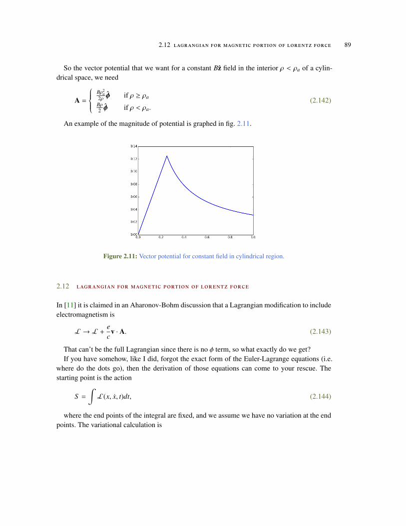
2.12 lagrangian for magnetic portion of lorentz force 89
So the vector potential that we want for a constant Bz field in the interior ρ < ρa of a cylin-drical space, we need
(2.142)A =
Bρ2
a2ρ φ if ρ ≥ ρa
Bρ2 φ if ρ < ρa.
An example of the magnitude of potential is graphed in fig. 2.11.
Figure 2.11: Vector potential for constant field in cylindrical region.
2.12 lagrangian for magnetic portion of lorentz force
In [11] it is claimed in an Aharonov-Bohm discussion that a Lagrangian modification to includeelectromagnetism is
(2.143)L → L +ec
v · A.
That can’t be the full Lagrangian since there is no φ term, so what exactly do we get?If you have somehow, like I did, forgot the exact form of the Euler-Lagrange equations (i.e.
where do the dots go), then the derivation of those equations can come to your rescue. Thestarting point is the action
(2.144)S =
∫L(x, x, t)dt,
where the end points of the integral are fixed, and we assume we have no variation at the endpoints. The variational calculation is

90 quantum dynamics
(2.145)
δS =
∫δL(x, x, t)dt
=
∫ (∂L
∂xδx +
∂L
∂xδx
)dt
=
∫ (∂L
∂xδx +
∂L
∂xδ
dxdt
)dt
=
∫ (∂L
∂x−
ddt
(∂L
∂x
))δxdt + δx
∂L
∂x.
The boundary term is killed after evaluation at the end points where the variation is zero. Forthe result to hold for all variations δx, we must have
∂L
∂x=
ddt
(∂L
∂x
). (2.146)
Now lets apply this to the Lagrangian at hand. For the position derivative we have
(2.147)∂L
∂xi=
ec
v j∂A j
∂xi.
For the canonical momentum term, assuming A = A(x) we have
(2.148)
ddt∂L
∂xi=
ddt
(mxi +
ec
Ai
)= mxi +
ec
dAi
dt
= mxi +ec∂Ai
∂x j
dx j
dt.
Assembling the results, we’ve got
(2.149)0 =
ddt∂L
∂xi−∂L
∂xi
= mxi +ec∂Ai
∂x j
dx j
dt−
ec
v j∂A j
∂xi,
or
(2.150)
mxi =ec
v j∂A j
∂xi−
ec∂Ai
∂x jv j
=ec
v j
(∂A j
∂xi−∂Ai
∂x j
)=
ec
v jBkεi jk.

2.13 problems 91
In vector form that is
mx =ec
v ×B. (2.151)
So, we get the magnetic term of the Lorentz force. Also note that this shows the Lagrangian(and the end result), was not in SI units. The 1/c term would have to be dropped for SI.
2.13 problems
Exercise 2.1 Lorentz force from classical electrodynamic Hamiltonian.Given the classical Hamiltonian
(2.152)H =1
2m(p − qA)2 + qφ.
apply the Hamiltonian equations of motion
dpdt
= −∂H∂q
dqdt
=∂H∂p
,
(2.153)
to show that this is the Hamiltonian that describes the Lorentz force equation, and to find thevelocity in terms of the canonical momentum and vector potential.Answer for Exercise 2.1
The particle velocity follows easily
(2.154)
v =drdt
=∂H∂p
=1m
(p − qA) .
For the Lorentz force we can proceed in the coordinate representation
(2.155)
dpk
dt= −
∂H∂xk
= −2
2m(pm − qAm)
∂
∂xk(pm − qAm) − q
∂φ
∂xk
= qvm∂Am
∂xk− q
∂φ
∂xk,

92 quantum dynamics
We also have
(2.156)
dpk
dt=
ddt
(mxk + qAk)
= md2xk
dt2 + q∂Ak
∂xm
dxm
dt+ q
∂Ak
∂t.
Putting these together we’ve got
(2.157)
md2xk
dt2 = qvm∂Am
∂xk− q
∂φ
∂xk,−q
∂Ak
∂xm
dxm
dt− q
∂Ak
∂t
= qvm
(∂Am
∂xk−∂Ak
∂xm
)+ qEk
= qvmεkmsBs + qEk,
or
(2.158)md2xdt2 = qekvmεkmsBs + qEk
= qv × B + qE.
Exercise 2.2 Show gauge invariance of the magnetic and electric fields.
After the gauge transformation of eq. (2.60) show that the electric and magnetic fields areunaltered.Answer for Exercise 2.2
For the magnetic field the transformed field is
(2.159)
B′ = ∇ × (A + ∇χ)= ∇ × A + ∇ × (∇χ)= ∇ × A= B.
(2.160)
E′ = −∂A′
∂t− ∇φ′
= −∂
∂t(A + ∇χ) − ∇
(φ −
∂χ
∂t
)= −
∂A∂t− ∇φ
= E.

2.13 problems 93
Exercise 2.3 Gauge transformation.
Show that after a transformation of position and momentum of the following form
(2.161)r′ = rp′ = p − q∇χ(r)
all the commutators have the expected values.Answer for Exercise 2.3
The position commutators don’t need consideration. Of interest is the momentum-positioncommutators
(2.162)
[p′k, x
′k
]=
[pk − q∂kχ, xk
]=
[pk, xk
]− q
[∂kχ, xk
]=
[pk, xk
],
and the momentum commutators
(2.163)
[p′k, p′j
]=
[pk − q∂kχ, p j − q∂ jχ
]=
[pk, p j
]− q
([∂kχ, p j
]+
[pk, ∂ jχ
]).
That last sum of commutators is
(2.164)[∂kχ, p j
]+
[pk, ∂ jχ
]= −i h
(∂(∂ jχ)∂k
−∂(∂kχ)∂ j
)= 0.
We’ve shown that
(2.165)[ p′k, x
′k] = [ pk, xk][
p′k, p′j]
= [ pk, p j] .
All the other commutators clearly have the desired transformation properties.
Exercise 2.4 Heisenberg picture spin precession. ([11] pr. 2.1)
For the spin Hamiltonian
(2.166)H = −eBmc
S z
= ωS z,
express and solve the Heisenberg equations of motion for S x(t), S y(t), and S z(t).

94 quantum dynamics
Answer for Exercise 2.4The equations of motion are of the form
(2.167)
dS Hi
dt=
1i h
[S H
i ,H]
=1i h
[U†S iU,H
]=
1i h
(U†S iUH − HU†S iU
)=
1i h
U† (S iH − HS i) U
=ω
i hU†
[S i, S z
]U.
These are
(2.168)
dS Hx
dt= −ωU†S yU
dS Hy
dt= ωU†S xU
dS Hz
dt= 0.
To completely specify these equations, we need to expand U(t), which is
(2.169)
U(t) = e−iHt/ h
= e−iωS zt/ h
= e−iωσzt/2
= cos (ωt/2) − iσz sin (ωt/2)
=
cos (ωt/2) − i sin (ωt/2) 0
0 cos (ωt/2) + i sin (ωt/2)
=
e−iωt/2 0
0 eiωt/2
.The equations of motion can now be written out in full. To do so seems a bit silly since we
also know that S Hx = U†S xU, S H
y U†S xU. However, if that is temporarily forgotten, we can showthat the Heisenberg equations of motion can be solved for these too.

2.13 problems 95
(2.170)
U†S xU =h2
eiωt/2 0
0 e−iωt/2
0 1
1 0
e−iωt/2 0
0 eiωt/2
=
h2
0 eiωt/2
e−iωt/2 0
e−iωt/2 0
0 eiωt/2
=
h2
0 eiωt
e−iωt 0
,and
(2.171)
U†S yU =h2
eiωt/2 0
0 e−iωt/2
0 −i
i 0
e−iωt/2 0
0 eiωt/2
=
i h2
0 −eiωt/2
e−iωt/2 0
e−iωt/2 0
0 eiωt/2
=
i h2
0 −eiωt
e−iωt 0
.The equations of motion are now fully specified
(2.172)
dS Hx
dt= −
i hω2
0 −eiωt
e−iωt 0
dS H
y
dt=
hω2
0 eiωt
e−iωt 0
dS H
z
dt= 0.
Integration gives
(2.173)
S Hx =
h2
0 eiωt
e−iωt 0
+ C
S Hy =
h2
0 −ieiωt
ie−iωt 0
+ C
S Hz = C.
The integration constants are fixed by the boundary condition S Hi (0) = S i, so

96 quantum dynamics
(2.174)
S Hx =
h2
0 eiωt
e−iωt 0
S H
y =i h2
0 −eiωt
e−iωt 0
S H
z = S z.
Observe that these integrated values S Hx , S
Hy match eq. (2.170), and eq. (2.171) as expected.
Exercise 2.5 Dynamics of non-Hermitian Hamiltonian. ([11] pr. 2.2)
Revisiting an earlier Hamiltonian, but assuming it was entered incorrectly as
(2.175)H = H11 |1〉 〈1| + H22 |2〉 〈2| + H12 |1〉 〈2| .
What principle is now violated? Illustrate your point explicitly by attempting to solve themost general time-dependent problem using an illegal Hamiltonian of this kind. You may as-sume that H11 = H22 for simplicity.Answer for Exercise 2.5
In matrix form this Hamiltonian is
(2.176)
H =
〈1|H |1〉 〈1|H |2〉〈2|H |1〉 〈2|H |2〉
=
H11 H12
0 H22
.This is not a Hermitian operator. What is the physical implication of this non-Hermicity?
Consider the simpler case where H11 = H22. Such a Hamiltonian has the form
(2.177)H =
a b
0 a
.This has only one unique eigenvector ( (1, 0), but we can still solve the time evolution equa-
tion
(2.178)i h∂U∂t
= HU,
since for constant H, we have
(2.179)U = e−iHt/ h.

2.13 problems 97
To exponentiate, note that we have
(2.180)
a b
0 a
n
=
an nan−1b
0 an
.To prove the induction, the n = 2 case follows easily
(2.181)
a b
0 a
a b
0 a
=
a2 2ab
0 a2
,as does the general case
(2.182)
an nan−1b
0 an
a b
0 a
=
an+1 (n + 1)anb
0 an+1
.The exponential sum is thus
(2.183)eHτ =
eaτ 0 + bτ1! + 2abτ2
2! + 3a2bτ3
3! + · · ·
0 eaτ
.That sum simplifies to
(2.184)
bτ0!
+abτ2
1!+
a2bτ3
2!+ · · ·
= bτ(1 +
aτ1!
+(aτ)2
2!+ · · ·
)= bτeaτ.
The exponential is thus
(2.185)
eHτ =
eaτ bτeaτ
0 eaτ
=
1 bτ
0 1
eaτ.
In particular
(2.186)U = e−iHt/ h
=
1 −ibt/ h
0 1
e−iat/ h.
98 quantum dynamics
We can verify that this is a solution to eq. (2.178). The left hand side is
(2.187)
i h∂U∂t
= i h
−ia/ h −ib/ h + (−ibt/ h)(−ia/ h)
0 −ia/ h
e−iat/ h
=
a b − iabt/ h
0 a
e−iat/ h,
and for the right hand side
(2.188)
HU =
a b
0 a
1 −ibt/ h
0 1
e−iat/ h
=
a b − iabt/ h
0 a
e−iat/ h
= i h∂U∂t.
While the Schrödinger is satisfied, we don’t have the unitary inversion physical property thatis desired for the time evolution operator U. Namely
(2.189)
U†U =
1 0
ibt/ h 1
eiat/ h
1 −ibt/ h
0 1
e−iat/ h
=
1 −ibt/ h
ibt/ h (bt)2/ h2
, I.
We required U†U = I for the time evolution operator, but don’t have that property for thisnon-Hermitian Hamiltonian.
Exercise 2.6 Time evolution of spin half probability and dispersion. ([11] pr. 2.3)A spin 1/2 system S · n, with n = sin βx + cos βz, is in state with eigenvalue h/2, acted on by
a magnetic field of strength B in the +z direction.
a. If S x is measured at time t, what is the probability of getting + h/2?
b. Evaluate the dispersion in S x as a function of t, that is,
⟨(S x − 〈S x〉)
2⟩. (2.190)
c. Check your answers for β→ 0, π/2 to see if they make sense.
Answer for Exercise 2.6

2.13 problems 99
Part a. The spin operator in matrix form is
(2.191)
S · n =h2
(σz cos β + σx sin β)
=h2
1 0
0 −1
cos β +
0 1
1 0
sin β
=
h2
cos β sin β
sin β − cos β
.The |S · n; +〉 eigenstate is found from
(2.192)(S · n − h/2)
ab = 0,
or
(2.193)
0 = (cos β − 1) a + sin βb=
(−2 sin2(β/2)
)a + 2 sin(β/2) cos(β/2)b
= (− sin(β/2)) a + cos(β/2)b,
or
(2.194)|S · n; +〉 =
cos(β/2)
sin(β/2)
.The Hamiltonian is
H = −eBmc
S z = −eB h2mc
σz, (2.195)
so the time evolution operator is
(2.196)U = e−iHt/ h
= eieBt2mcσz .
Let ω = eB/(2mc), so
(2.197)
U = eiσzωt
= cos(ωt) + iσz sin(ωt)
=
1 0
0 1
cos(ωt) + i
1 0
0 −1
sin(ωt)
=
eiωt 0
0 e−iωt
.

100 quantum dynamics
The time evolution of the initial state is
(2.198)
|S · n; +〉 (t) = U |S · n; +〉 (0)
=
eiωt 0
0 e−iωt
cos(β/2)
sin(β/2)
=
cos(β/2)eiωt
sin(β/2)e−iωt
.The probability of finding the state in |S · x; +〉 at time t (i.e. measuring S x and finding h/2)
is
(2.199)
|〈S · x; +|S · n; +〉|2 =
∣∣∣∣∣∣∣ 1√
2
[1 1
] cos(β/2)eiωt
sin(β/2)e−iωt
∣∣∣∣∣∣∣2
=12
∣∣∣cos(β/2)eiωt + sin(β/2)e−iωt∣∣∣2
=12(1 + 2 cos(β/2) sin(β/2) cos(2ωt))
=12(1 + sin(β) cos(2ωt)) .
Part b. To calculate the dispersion first note that
(2.200)S 2
x =
(h2
)20 1
1 0
2
=
(h2
)2
,
so only the first order expectation is non-trivial to calculate. That is
(2.201)
〈S x〉 =h2
[cos(β/2)e−iωt sin(β/2)eiωt
] 0 1
1 0
cos(β/2)eiωt
sin(β/2)e−iωt
=
h2
[cos(β/2)e−iωt sin(β/2)eiωt
] sin(β/2)e−iωt
cos(β/2)eiωt
=
h2
sin(β/2) cos(β/2)(e−2iωt + e2iωt
)=
h2
sin β cos(2ωt).
This gives

2.13 problems 101
⟨(∆S x)2
⟩=
(h2
)2 (1 − sin2 β cos2(2ωt)
)(2.202)
Part c. For β = 0, n = z, and β = π/2, n = x. For the first case, the state is in an eigenstate ofS z, so must evolve as
(2.203)|S · n; +〉 (t) = |S · n; +〉 (0)eiωt.
The probability of finding it in state |S · x; +〉 is therefore
(2.204)
∣∣∣∣∣∣∣ 1√
2
[1 1
] eiωt
0
∣∣∣∣∣∣∣2
=12
∣∣∣eiωt∣∣∣2
=12
=12
(1 + sin(0) cos(2ωt)) .
This matches eq. (2.199) as expected.For β = π/2 we have
(2.205)
|S · x; +〉 (t) =1√
2
eiωt 0
0 e−iωt
11
=
1√
2
eiωt
e−iωt
.The probability for the h/2 S x measurement at time t is
(2.206)
∣∣∣∣∣∣∣12 [1 1
] eiωt
e−iωt
∣∣∣∣∣∣∣2
=14
∣∣∣eiωt + e−iωt∣∣∣2
= cos2(ωt)
=12
(1 + sin(π/2) cos(2ωt)) .
Again, this matches the expected value.For the dispersions, at β = 0, the dispersion is
(2.207)(
h2
)2

102 quantum dynamics
This is the maximum dispersion, which makes sense since we are measuring S x when theinitial state is |S · z; +〉. For β = π/2 the dispersion is
(2.208)(
h2
)2
sin2(2ωt).
This starts off as zero dispersion (because the initial state is |S · x; +〉, but then oscillates.
Exercise 2.7 Heisenberg picture position commutator. ([11] pr. 2.5)
Evaluate
(2.209)[x(t), x(0)] ,
for a Heisenberg picture operator x(t) for a free particle.Answer for Exercise 2.7
The free particle Hamiltonian is
(2.210)H =p2
2m,
so the time evolution operator is
(2.211)U(t) = e−ip2t/(2m h).
The Heisenberg picture position operator is

2.13 problems 103
(2.212)
xH = U†xU= eip2t/(2m h)xe−ip2t/(2m h)
=
∞∑k=0
1k!
(ip2t2m h
)k
xe−ip2t/(2m h)
=
∞∑k=0
1k!
( it2m h
)kp2kxe−ip2t/(2m h)
=
∞∑k=0
1k!
( it2m h
)k ([p2k, x
]+ xp2k
)e−ip2t/(2m h)
= x +
∞∑k=0
1k!
( it2m h
)k [p2k, x
]e−ip2t/(2m h)
= x +
∞∑k=0
1k!
( it2m h
)k (−i h
∂p2k
∂p
)e−ip2t/(2m h)
= x +
∞∑k=0
1k!
( it2m h
)k (−i h2kp2k−1
)e−ip2t/(2m h)
= x + −2i hpit
2m h
∞∑k=1
1(k − 1)!
( it2m h
)k−1p2(k−1)e−ip2t/(2m h)
= x + tpm.
This has the structure of a classical free particle x(t) = x + vt, but in this case x, p are opera-tors.
The evolved position commutator is
(2.213)
[x(t), x(0)] =[x + tp/m, x
]=
tm
[p, x
]= −i h
tm.
Compare this to the classical Poisson bracket
(2.214)[x(t), x(0)]classical =
∂
∂x(x + pt/m)
∂x∂p−
∂
∂p(x + pt/m)
∂x∂x
= −tm.
This has the expected relation [x(t), x(0)] = i h [x(t), x(0)]classical.

104 quantum dynamics
Exercise 2.8 Virial theorem. (phy1520 2015 ps2.2)Consider a three-dimensional Hamiltonian
(2.215)H =p2
2m+ V(x).
a. Calculate [x · p,H] and show that
(2.216)ddt〈x · p〉 =
⟨p2
m
⟩− 〈x · ∇V〉 .
When the l.h.s. vanishes, the result that the r.h.s. is zero is called the quantum virialtheorem.
b. Consider the 3D isotropic harmonic oscillator, and show explicitly that its eigenstatesobey the virial theorem.
c. Evaluate the r.h.s. for the superposition state |0, 0, 0〉+ |0, 0, 2〉 where the notation standsfor
∣∣∣nx, ny, nz⟩
occupation numbers.
d. Under what conditions does the left-hand side vanish?Answer for Exercise 2.8
PROBLEM SET RELATED MATERIAL REDACTED IN THIS DOCUMENT.PLEASEFEEL FREE TO EMAIL ME FOR THE FULL VERSION IF YOU AREN’T TAKING PHY1520.
. .. .
.. . .
. .. . .
. .. .
. END-REDACTION
Exercise 2.9 A symmetric real Hamiltonian. ([11] pr. 2.9)Find the time evolution for the state |a′〉 for a Hamiltonian of the form
(2.217)H = δ(∣∣∣a′⟩ ⟨a′∣∣∣ +
∣∣∣a′′⟩ ⟨a′′∣∣∣)Answer for Exercise 2.9
This Hamiltonian has the matrix representation
(2.218)H =
0 δ
δ 0
,

2.13 problems 105
which has a characteristic equation of
(2.219)λ2 − δ2 = 0,
so the energy eigenvalues are ±δ.The diagonal basis states are respectively
(2.220)|±δ〉 =1√
2
±1
1
.The time evolution operator is
(2.221)
U = e−iHt/ h
= e−iδt/ h |+δ〉 〈+δ| + eiδt/ h |−δ〉 〈−δ|
=e−iδt/ h
2
[1 1
] 11 +
eiδt/ h
2
[−1 1
] −1
1
=
e−iδt/ h
2
1 1
1 1
+eiδt/ h
2
1 −1
−1 1
=
cos(δt/ h) −i sin(δt/ h)
−i sin(δt/ h) cos(δt/ h)
.The desired time evolution in the original basis is
(2.222)
∣∣∣a′, t⟩ = e−iHt/ h∣∣∣a′, 0⟩
=
cos(δt/ h) −i sin(δt/ h)
−i sin(δt/ h) cos(δt/ h)
10
=
cos(δt/ h)
−i sin(δt/ h)
= cos(δt/ h)
∣∣∣a′, 0⟩ − i sin(δt/ h)∣∣∣a′′, 0⟩ .
This evolution has the same structure as left circularly polarized light.The probability of finding the system in state |a′′〉 given an initial state of |a′, 0〉 is
(2.223)P =∣∣∣⟨a′′∣∣∣a′, t⟩∣∣∣2
= sin2 (δt/ h) .

106 quantum dynamics
Exercise 2.10 SHO translation operator expectation. ([11] pr. 2.12)
Using the Heisenberg picture evaluate the expectation of the position operator 〈x〉 with re-spect to the initial time state
(2.224)|α, 0〉 = e−ip0a/ h |0〉 ,
where p0 is the initial time position operator, and a is a constant with dimensions of position.Answer for Exercise 2.10
Recall that the Heisenberg picture position operator expands to
(2.225)xH(t) = U†xU
= x0 cos(ωt) +p0
mωsin(ωt),
so the expectation of the position operator is
(2.226)〈x〉 = 〈0| eip0a/ h
(x0 cos(ωt) +
p0
mωsin(ωt)
)e−ip0a/ h |0〉
= 〈0|(eip0a/ hx0 cos(ωt)e−ip0a/ h cos(ωt) +
p0
mωsin(ωt)
)|0〉 .
The exponential sandwich above can be expanded using the Baker-Campbell-Hausdorff [15]formula
(2.227)
eip0a/ hx0e−ip0a/ h = x0 +iah[p0, x0] +
12!
( iah
)2[p0, [p0, x0]] + · · ·
= x0 +iah(−i h) +
12!
( iah
)2[p0,−i h] + · · ·
= x0 + a.
The position expectation with respect to this translated state is
(2.228)〈x〉 = 〈0|((x0 + a) cos(ωt) +
p0
mωsin(ωt)
)|0〉
= a cos(ωt).
The final simplification above follows from 〈n| x |n〉 = 〈n| p |n〉 = 0.
Exercise 2.11 Expectations for SHO Hamiltonian, and virial theorem. ([11] pr. 2.14)
a. For a 1D SHO, compute 〈m| x |n〉 , 〈m| x2 |n〉 , 〈m| p |n〉 , 〈m| p2 |n〉 and 〈m| x, p |n〉.
b. Verify the virial theorem is satisfied for energy eigenstates.
Answer for Exercise 2.11

2.13 problems 107
Part a. Using
x =x0√
2
(a + a†
)p =
i h
x0√
2
(a† − a
)a(t) = a(0)e−iωt
a(0) |n〉 =√
n |n − 1〉
a†(0) |n〉 =√
n + 1 |n + 1〉
x20 =
hωm
,
(2.229)
we have
(2.230)
〈m| x |n〉 =x0√
2〈m|
(a + a†
)|n〉
=x0√
2〈m|
(e−iωt √n |n − 1〉 + eiωt
√n + 1 |n + 1〉
)=
x0√
2
(δm,n−1e−iωt √n + δm,n+1eiωt
√n + 1
),
〈m| x2 |n〉 =x2
0
2〈m|
(a + a†
)2|n〉
=x2
0
2
(eiωt √m 〈m − 1| + e−iωt
√m + 1 〈m + 1|
) (e−iωt √n |n − 1〉 + eiωt
√n + 1 |n + 1〉
)=
x20
2
(δm+1,n+1
√(m + 1)(n + 1)
+ δm+1,n−1√
(m + 1)ne−2iωt + δm−1,n+1√
m(n + 1)e2iωt + δm−1,n−1√
mn),
(2.231)
(2.232)
〈m| p |n〉 =i h√
2x0〈m|
(a† − a
)|n〉
=i h√
2x0〈m|
(eiωt√
n + 1 |n + 1〉 − e−iωt √n |n − 1〉)
=i h√
2x0
(δm,n+1eiωt
√n + 1 − δm,n−1e−iωt √n
),

108 quantum dynamics
〈m| p2 |n〉 =h2
2x20
|m〉(a − a†
) (a† − a
)|n〉
=h2
2x20
(−e−iωt
√m + 1 〈m + 1|+eiωt √m 〈m − 1|
) (eiωt√
n + 1 |n + 1〉−e−iωt √n |n − 1〉)
=h2
2x20
(δm+1,n+1
√(m + 1)(n + 1)
+ δm+1,n−1√
(m + 1)ne−2iωt + δm−1,n+1√
m(n + 1)e2iωt + δm−1,n−1√
mn).
(2.233)
For the anticommutator x, p, we have
(2.234)
x, p =i h2
((ae−iωt + a†eiωt
) (a†eiωt − ae−iωt
)−
(a†eiωt − ae−iωt
) (ae−iωt + a†eiωt
))=
i h2
(−a2e−2iωt + (a†)2e2iωt + aa† − a†a + a2e−2iωt − (a†)2e2iωt − a†a + aa†
)= i h
(aa† − a†a
),
so
(2.235)
〈m| x, p |n〉 = i h 〈m|(aa† − a†a
)|n〉
= i h 〈m|( √
(n + 1)2 |n〉 −√
n2 |n〉)
= i h 〈m| (2n + 1) |n〉 .
Part b. For the SHO, the virial theorem requires⟨p2/m
⟩=
⟨mωx2
⟩. That momentum expec-
tation with respect to the eigenstate |n〉 is
(2.236)⟨p2/m
⟩=
h2
2x20m
( √(n + 1)(n + 1) +
√nn
)=
h2mω2 hm
(2n + 1) = hω(n +
12
).
For the position expectation we’ve got
(2.237)
⟨mωx2
⟩=
mω2x20
2
( √(n + 1)(n + 1) +
√nn
)=
mω2 h2mω
( √(n + 1)(n + 1) +
√nn
)=ω h2
(2n + 1)
= ω h(n +
12
).
This shows that the virial theorem holds for the SHO Hamiltonian for eigenstates.

2.13 problems 109
Exercise 2.12 Momentum space representation of Schrödinger equation. ([11] pr. 2.15)
Using
(2.238)⟨x′∣∣∣p′⟩ =
1√
2π heip′x′/ h,
show that
(2.239)⟨p′
∣∣∣ x |α〉 = i h∂
∂p′⟨p′
∣∣∣α⟩ .Use this to find the momentum space representation of the Schrödinger equation for the one
dimensional SHO and the energy eigenfunctions in their momentum representation.Answer for Exercise 2.12
To expand the matrix element, introduce both momentum and position space identity opera-tors
(2.240)
⟨p′
∣∣∣ x |α〉 =
∫dx′dp′′
⟨p′
∣∣∣x′⟩ ⟨x′∣∣∣ x
∣∣∣p′′⟩ ⟨p′′∣∣∣α⟩
=
∫dx′dp′′
⟨p′
∣∣∣x′⟩ x′⟨x′∣∣∣p′′⟩ ⟨p′′
∣∣∣α⟩=
12π h
∫dx′dp′′e−ip′x′/ hx′eip′′x′/ h ⟨
p′′∣∣∣α⟩
=1
2π h
∫dx′dp′′x′ei(p′′−p′)x′/ h ⟨
p′′∣∣∣α⟩
=1
2π h
∫dx′dp′′
ddp′′
(−i h
e
i(p′′−p′)x′/ h) ⟨p′′
∣∣∣α⟩= i h
∫dp′′
(1
2π h
∫dx′ei(p′′−p′)x′/ h
)d
dp′′⟨p′′
∣∣∣α⟩= i h
∫dp′′δ(p′′ − p′)
ddp′′
⟨p′′
∣∣∣α⟩= i h
ddp′
⟨p′
∣∣∣α⟩ .
Schrödinger’s equation for a time dependent state |α〉 = U(t) |α, 0〉 is
(2.241)i h∂
∂t|α〉 = H |α〉 ,
with the momentum representation
(2.242)i h∂
∂t⟨p′
∣∣∣α⟩ =⟨p′
∣∣∣ H |α〉 .

110 quantum dynamics
Expansion of the Hamiltonian matrix element for a strictly spatial dependent potential V(x)gives
(2.243)
⟨p′
∣∣∣ H |α〉 =⟨p′
∣∣∣ ( p2
2m+ V(x)
)|α〉
=(p′)2
2m+
⟨p′
∣∣∣ V(x) |α〉 .
Assuming a Taylor representation of the potential V(x) =∑
ckxk, we want to calculate
(2.244)⟨p′
∣∣∣ V(x) |α〉 =∑
ck⟨p′
∣∣∣ xk |α〉 .
With |α〉 = |p′′〉 eq. (2.239) provides the k = 1 term
(2.245)
⟨p′
∣∣∣ x∣∣∣p′′⟩ = i h
ddp′
⟨p′
∣∣∣p′′⟩= i h
ddp′
δ(p′ − p′′),
where it is implied here that the derivative is operating on not just the delta function, but onall else that follows.
Using this the higher powers of 〈p′| xk |α〉 can be found easily. For example for k = 2 we have
(2.246)
⟨p′
∣∣∣ x2 |α〉 =
∫dp′′
⟨p′
∣∣∣ x∣∣∣p′′⟩ ⟨p′′
∣∣∣ x |α〉
=
∫dp′′i h
ddp′
δ(p′ − p′′)i hd
dp′′⟨p′′
∣∣∣α⟩= (i h)2 d2
d(p′)2
⟨p′
∣∣∣α⟩ .This means that the potential matrix element is
(2.247)
⟨p′
∣∣∣ V(x) |α〉 =∑
ck
(i h
ddp′
)k ⟨p′
∣∣∣α⟩= V
(i h
ddp′
).
Writing Ψα(p′) = 〈p′|α〉, the momentum space representation of Schrödinger’s equation fora position dependent potential is
i h∂
∂tΨα(p′) =
((p′)2
2m+ V (i h∂/∂p′)
)Ψα(p′). (2.248)

2.13 problems 111
For the SHO Hamiltonian the potential is V(x) = (1/2)mω2x2, so the Schrödinger equationis
(2.249)i h∂
∂tΨα(p′) =
((p′)2
2m−
12
mω2 h2 ∂2
∂(p′)2
)Ψα(p′)
=1
2m
((p′)2 − m2ω2 h2 ∂2
∂(p′)2
)Ψα(p′).
To determine the wave functions, let’s non-dimensionalize this and compare to the positionspace Schrödinger equation. Let
(2.250)p20 = mωh,
so
(2.251)i h∂
∂tΨα(p′) =
p20
2m
( p′
p0
)2
−∂2
∂(p′/p0)2
Ψα(p′)
=ω h2
− ∂2
∂(p′/p0)2 +
(p′
p0
)2 Ψα(p′).
Compare this to the position space equation with x20 = mω/ h,
(2.252)
i h∂
∂tΨα(x′) =
(−
h2
2m∂2
∂(x′)2 +12
mω2(x′)2)
Ψα(x′)
=h2
2m
(−
∂2
∂(x′)2 +m2ω2
h2 (x′)2)
Ψα(x′)
=h2x2
0
2m
− ∂2
∂(x′/x0)2 +
(x′
x0
)2 Ψα(x′)
=hω2
− ∂2
∂(x′/x0)2 +
(x′
x0
)2 Ψα(x′).
It’s clear that there is a straightforward duality relationship between the respective wavefunctions. Since
(2.253)⟨x′∣∣∣n⟩ =
1
π1/4√
2nn!xn+1/20
(x′ − x2
0d
dx′
)n
exp
−12
(x′
x0
)2 ,the momentum space wave functions are
(2.254)⟨p′
∣∣∣n⟩ =1
π1/4√
2nn!pn+1/20
(p′ − p2
0d
dp′
)n
exp
−12
(p′
p0
)2 .

112 quantum dynamics
Exercise 2.13 Correlation function. (phy1520 2015 ps2.3)
Consider 〈x(0)x(t)〉 and 〈p(0)p(t)〉 where operators are in the Heisenberg representation.These are called correlation functions. Evaluate this for the 1D harmonic oscillator in an en-ergy eigenstate |n〉.Answer for Exercise 2.13
PROBLEM SET RELATED MATERIAL REDACTED IN THIS DOCUMENT.PLEASEFEEL FREE TO EMAIL ME FOR THE FULL VERSION IF YOU AREN’T TAKING PHY1520.
. .. .
.. . .
. .. . .
. .. .
. END-REDACTION
Exercise 2.14 1D SHO linear superposition that maximizes expectation. ([11] pr. 2.17)
For a 1D SHO
a. Construct a linear combination of |0〉 , |1〉 that maximizes 〈x〉 without using wave func-tions.
b. How does this state evolve with time?
c. Evaluate 〈x〉 using the Schrödinger picture.
d. Evaluate 〈x〉 using the Heisenberg picture.
e. Evaluate⟨(∆x)2
⟩.
Answer for Exercise 2.14
Part a. Forming
(2.255)|ψ〉 =|0〉 + σ |1〉√
1 + |σ|2
the position expectation is
(2.256)〈ψ| x |ψ〉 =1
1 + |σ|2(〈0| + σ∗ 〈1|
) x0√
2
(a† + a
)(|0〉 + σ |1〉) .
Evaluating the action of the operators on the kets, we’ve got

2.13 problems 113
(2.257)(a† + a
)(|0〉 + σ |1〉) = |1〉 +
√2σ |2〉 + σ |0〉 .
The |2〉 term is killed by the bras, leaving
(2.258)〈x〉 =
11 + |σ|2
x0√
2
(σ + σ∗
)=
√2x0 Reσ1 + |σ|2
.
Any imaginary component in σ will reduce the expectation, so we are constrained to pickinga real value.
The derivative of
(2.259)f (σ) =σ
1 + σ2 ,
is
(2.260)f ′(σ) =1 − σ2
(1 + σ2)2 .
That has zeros at σ = ±1. The second derivative is
(2.261)f ′′(σ) =−2σ(3 − σ2)
(1 + σ2)3 .
That will be negative (maximum for the extreme value) at σ = 1, so the linear superpositionof these first two energy eigenkets that maximizes the position expectation is
(2.262)ψ =1√
2(|0〉 + |1〉) .
That maximized position expectation is
(2.263)〈x〉 =x0√
2.
Part b. The time evolution is given by
(2.264)
|Ψ(t)〉 = e−iHt/ h 1√
2(|0〉 + |1〉)
=1√
2
(e−i(0+1/2) hωt/ h |0〉 + e−i(1+1/2) hωt/ h |1〉
)=
1√
2
(e−iωt/2 |0〉 + e−3iωt/2 |1〉
).

114 quantum dynamics
Part c. The position expectation in the Schrödinger representation is
(2.265)
〈x(t)〉 =12
(eiωt/2 〈0| + e3iωt/2 〈1|
) x0√
2
(a† + a
) (e−iωt/2 |0〉 + e−3iωt/2 |1〉
)=
x0
2√
2
(eiωt/2 〈0| + e3iωt/2 〈1|
) (e−iωt/2 |1〉 + e−3iωt/2
√2 |2〉 + e−3iωt/2 |0〉
)=
x0√
2cos(ωt).
Part d.
(2.266)
〈x(t)〉 =12
(〈0| + 〈1|)x0√
2
(a†eiωt + ae−iωt
)(|0〉 + |1〉)
=x0
2√
2(〈0| + 〈1|)
(eiωt |1〉 +
√2eiωt |2〉 + e−iωt |0〉
)=
x0√
2cos(ωt),
matching the calculation using the Schrödinger picture.
Part e. Let’s use the Heisenberg picture for the uncertainty calculation. Using the calculationabove we have
(2.267)
⟨x2
⟩=
12
x20
2
(e−iωt 〈1| +
√2e−iωt 〈2| + eiωt 〈0|
) (eiωt |1〉 +
√2eiωt |2〉 + e−iωt |0〉
)=
x20
4(1 + 2 + 1)
= x20.
The uncertainty is
(2.268)
⟨(∆x)2
⟩=
⟨x2
⟩− 〈x〉2
= x20 −
x20
2cos2(ωt)
=x2
0
2
(2 − cos2(ωt)
)=
x20
2
(1 + sin2(ωt)
)

2.13 problems 115
Exercise 2.15 Plane wave ground state expectation for 1D SHO. ([11] pr. 2.18)
For a 1D SHO, show that
(2.269)〈0| eikx |0〉 = exp(−k2 〈0| x2 |0〉 /2
).
Answer for Exercise 2.15Despite the simple appearance of this problem, I found this quite involved to show. To do so,
start with a series expansion of the expectation
(2.270)〈0| eikx |0〉 =
∞∑m=0
(ik)m
m!〈0| xm |0〉 .
Let
(2.271)X =(a + a†
),
so that
x =
√h
2ωmX =
x0√
2X. (2.272)
Consider the first few values of 〈0| Xn |0〉
(2.273)〈0| X |0〉 = 〈0|
(a + a†
)|0〉
= 〈0|1〉= 0,
(2.274)〈0| X2 |0〉 = 〈0|
(a + a†
)2|0〉
= 〈1|1〉= 1,
(2.275)〈0| X3 |0〉 = 〈0|
(a + a†
)3|0〉
= 〈1|(√
2 |2〉 + |0〉)
= 0.
Whenever the power n in Xn is even, the braket can be split into a bra that has only contri-butions from odd eigenstates and a ket with even eigenstates. We conclude that 〈0| Xn |0〉 = 0when n is odd.

116 quantum dynamics
Noting that 〈0| x2 |0〉 = x20/2, this leaves
(2.276)
〈0| eikx |0〉 =
∞∑m=0
(ik)2m
(2m)!〈0| x2m |0〉
=
∞∑m=0
(ik)2m
(2m)!
x20
2
m
〈0| X2m |0〉
=
∞∑m=0
1(2m)!
(−k2 〈0| x2 |0〉
)m〈0| X2m |0〉 .
This problem is now reduced to showing that
(2.277)1
(2m)!〈0| X2m |0〉 =
1m! 2m ,
or
(2.278)
〈0| X2m |0〉 =(2m)!m! 2m
=(2m)(2m − 1)(2m − 2) · · · (2)(1)
2mm!
=2m(m)(2m − 1)(m − 1)(2m − 3)(m − 2) · · · (2)(3)(1)(1)
2mm!= (2m − 1)! ! ,
where n! ! = n(n − 2)(n − 4) · · ·.It looks like 〈0| X2m |0〉 can be expanded by inserting an identity operator and proceeding
recursively, like
(2.279)〈0| X2m |0〉 = 〈0| X2
∞∑n=0
|n〉 〈n|
X2m−2 |0〉
= 〈0| X2 (|0〉 〈0| + |2〉 〈2|) X2m−2 |0〉= 〈0| X2m−2 |0〉 + 〈0| X2 |2〉 〈2| X2m−2 |0〉 .
This has made use of the observation that 〈0| X2 |n〉 = 0 for all n , 0, 2. The remaining termincludes the factor
(2.280)〈0| X2 |2〉 = 〈0|
(a + a†
)2|2〉
=(〈0| +
√2 〈2|
)|2〉
=√
2,

2.13 problems 117
Since√
2 |2〉 =(a†
)2|0〉, the expectation of interest can be written
(2.281)〈0| X2m |0〉 = 〈0| X2m−2 |0〉 + 〈0| a2X2m−2 |0〉 .
How do we expand the second term. Let’s look at how a and X commute
(2.282)
aX = [a, X] + Xa=
[a, a + a†
]+ Xa
=[a, a†
]+ Xa
= 1 + Xa,
(2.283)
a2X = a (aX)= a (1 + Xa)= a + aXa= a + (1 + Xa) a= 2a + Xa2.
Proceeding to expand a2Xn we find
a2X3 = 6X + 6X2a + X3a2
a2X4 = 12X2 + 8X3a + X4a2
a2X5 = 20X3 + 10X4a + X5a2
a2X6 = 30X4 + 12X5a + X6a2.
(2.284)
It appears that we have[a2Xn, Xna2
]= βnXn−2 + 2nXn−1a, (2.285)
where
βn = βn−1 + 2(n − 1), (2.286)
and β2 = 2. Some goofing around shows that βn = n(n − 1), so the induction hypothesis is
[a2Xn, Xna2
]= n(n − 1)Xn−2 + 2nXn−1a. (2.287)

118 quantum dynamics
Let’s check the induction
(2.288)
a2Xn+1 = a2XnX=
(n(n − 1)Xn−2 + 2nXn−1a + Xna2
)X
= n(n − 1)Xn−1 + 2nXn−1aX + Xna2X= n(n − 1)Xn−1 + 2nXn−1 (1 + Xa) + Xn
(2a + Xa2
)= n(n − 1)Xn−1 + 2nXn−1 + 2nXna + 2Xna + Xn+1a2
= Xn+1a2 + (2 + 2n)Xna + (2n + n(n − 1)) Xn−1
= Xn+1a2 + 2(n + 1)Xna + (n + 1)nXn−1,
which concludes the induction, giving
(2.289)〈0| a2Xn |0〉 = n(n − 1) 〈0| Xn−2 |0〉 ,
and
(2.290)〈0| X2m |0〉 = 〈0| X2m−2 |0〉 + (2m − 2)(2m − 3) 〈0| X2m−4 |0〉 .
Let
(2.291)σn = 〈0| Xn |0〉 ,
so that the recurrence relation, for 2n ≥ 4 is
(2.292)σ2n = σ2n−2 + (2n − 2)(2n − 3)σ2n−4
We want to show that this simplifies to
(2.293)σ2n = (2n − 1)! !
The first values are
σ0 = 〈0| X0 |0〉 = 1 (2.294a)
σ2 = 〈0| X2 |0〉 = 1 (2.294b)
which gives us the right result for the first term in the induction
(2.295)σ4 = σ2 + 2 × 1 × σ0
= 1 + 2= 3! !

2.13 problems 119
For the general induction term, consider
(2.296)
σ2n+2 = σ2n + 2n(2n − 1)σ2n−2
= (2n − 1)! ! +2n(2n − 1)(2n − 3)! != (2n + 1)(2n − 1)! != (2n + 1)! ! ,
which completes the final induction. That was also the last thing required to complete theproof, so we are done!
Exercise 2.16 Relation of probability flux to momentum.Show that the probability flux
(2.297)j(x, t) = −i h2m
(ψ∗∇ψ − ψ∇ψ∗
),
is related to the momentum expectation at a given time by the integral of the flux over allspace
(2.298)∫
d3xj(x, t) =〈p〉tm
.
Answer for Exercise 2.16This can be seen by recasting the integral in bra-ket form. Let
(2.299)ψ(x, t) = 〈x|ψ(t)〉 ,
and note that the momentum portions of the flux can be written as
(2.300)−i h∇ψ(x, t) = 〈x|p |ψ(t)〉 .
The current is therefore
(2.301)
j(x, t) =1
2m(ψ∗ 〈x|p |ψ(t)〉 + ψ〈x|p |ψ(t)〉∗
)=
12m
(〈x|ψ(t)〉∗ 〈x|p |ψ(t)〉 + 〈x|ψ(t)〉 〈x|p |ψ(t)〉∗
)=
12m
(〈ψ(t)|x〉 〈x|p |ψ(t)〉 + 〈ψ(t)|p |x〉 〈x|ψ(t)〉) .
Integrating and noting that the spatial identity is 1 =∫
d3x |x〉 〈x|, we have
(2.302)∫
d3xj(x, t) = 〈ψ(t)|p |ψ(t)〉 ,
This is just the expectation of p with respect to a specific time-instance state, demonstratingthe desired relationship.

120 quantum dynamics
Exercise 2.17 Hermite polynomial normalization constant. ([11] pr. 2.21)
Derive the normalization constant cn for the Harmonic oscillator solution
(2.303)un(x) = cnHn
(x√
mωh
)e−mωx2/2 h,
by deriving the orthogonality relationship using generating functions
g(x, t) = e−t2+2tx =
∞∑n=0
Hn(x)tn
n!. (2.304)
Start by working out the integral
I =
∫ ∞
−∞
g(x, t)g(x, s)e−x2dx, (2.305)
consider the integral twice with each side definition of the generating function.Answer for Exercise 2.17
First using the exponential definition of the generating function
(2.306)
∫ ∞
−∞
g(x, t)g(x, s)e−x2dx =
∫ ∞
−∞
e−t2+2txe−s2+2sxe−x2dx
= e−t2−s2∫ ∞
−∞
e−(x2−2tx−2sx)dx
= e−t2−s2+(s+t)2∫ ∞
−∞
e−(x−t−s)2dx
= e2st∫ ∞
−∞
e−u2du
=√πe2st.
With the Hermite polynomial definition of the generating function, this integral is
(2.307)
∫ ∞
−∞
g(x, t)g(x, s)e−x2dx =
∫ ∞
−∞
∞∑n=0
Hn(x)tn
n!
∞∑m=0
Hm(x)sm
m!e−x2
dx
=
∞∑n=0
tn
n!
∞∑m=0
sm
m!
∫ ∞
−∞
Hn(x)Hm(x)e−x2dx.
Let

2.13 problems 121
(2.308)αnm =
∫ ∞
−∞
Hn(x)Hm(x)e−x2dx,
and equate the two expansions of this integral
(2.309)√π
∞∑n =0
(2st)n
n!=
∞∑n=0
tn
n!
∞∑m=0
sm
m!αnm,
or, after equating powers of tn
(2.310)√π(2s)n =
∞∑m=0
sm
m!αnm.
This requires αnm to be zero for n , m, so
(2.311)√π2n =
1n!αnn,
and
(2.312)∫ ∞
−∞
Hn(x)Hm(x)e−x2dx = δnm
√π2nn! .
The SHO normalization is fixed by
(2.313)
∫ ∞
−∞
u2n(x)dx = c2
n
∫ ∞
−∞
H2n(x/x0)e−(x/x0)2
dx
= c2nx0√π2nn! ,
or
(2.314)
cn =1√
√π2nn!
√h
mω
=
(mωhπ
)1/42−n/2 1
√n!
Exercise 2.18 Dirac delta function potential. ([11] pr. 2.24,2.25)Given a Dirac delta function potential
(2.315)H =p2
2m− V0δ(x),
which vanishes after t = 0.
a. Solve for the bound state for t < 0,
b. Solve for the time evolution after that.Answer for Exercise 2.18

122 quantum dynamics
Part a. This problem can be solved directly by considering the |x| > 0 and x = 0 regionsseparately.
For |x| > 0 Schrödinger’s equation takes the form
(2.316)Eψ = −h2
2md2ψ
dx2 .
With
(2.317)κ =
√−2mE
h,
this has solutions
(2.318)ψ = e±κx.
For x > 0 we must have
(2.319)ψ = ae−κx,
and for x < 0
(2.320)ψ = beκx.
requiring that ψ is continuous at x = 0 means a = b, or
(2.321)ψ = ψ(0)e−κ|x|.
For the x = 0 region, consider an interval [−ε, ε] region around the origin. We must have
(2.322)E∫ ε
−εψ(x)dx =
− h2
2m
∫ ε
−ε
d2ψ
dx2 dx − V0
∫ ε
−εδ(x)ψ(x)dx.
The RHS is zero
(2.323)E∫ ε
−εψ(x)dx = E
e−κ(ε) − 1−κ
− E1 − eκ(−ε)
κ→ 0.
That leaves
(2.324)
V0
∫ ε
−εδ(x)ψ(x)dx =
− h2
2m
∫ ε
−ε
d2ψ
dx2 dx
=− h2
2mdψdx
∣∣∣∣∣ε−ε
=− h2
2mψ(0)
(−κe−κ(ε) − κeκ(−ε)
).

2.13 problems 123
In the ε → 0 limit this gives
(2.325)V0 =h2κ
m.
Equating relations for κ we have
κ =mV0
h2 =
√−2mE
h, (2.326)
or
E = −1
2m
(mV0
h
)2, (2.327)
with
ψ(x, t < 0) = C exp (−iEt/h − κ|x|) . (2.328)
The normalization requires
(2.329)
1 = 2|C|2∫ ∞
0e−2κxdx
= 2|C|2e−2κx
−2κ
∣∣∣∣∣∣∞0
=|C|2
κ,
so
ψ(x, t < 0) =√κ exp (−iEt/h − κ|x|) . (2.330)
There is only one bound state for such a potential.
Part b. After turning off the potential, any plane wave
ψ(x, t) = eikx−iE(k)t/ h, (2.331)
where
k =
√2mEh
, (2.332)

124 quantum dynamics
is a solution. In particular, at t = 0, the wave packet
ψ(x, 0) =1√
2π
∫ ∞
−∞
eikxA(k)dk, (2.333)
is a solution. To solve for A(k), we require
(2.334)1√
2π
∫ ∞
−∞
eikxA(k)dk =√κe−κ|x|,
or
A(k) =
√κ
2π
∫ ∞
−∞
e−ikxe−κ|x|dx =
√2π
κ3/2
κ2 + k2 . (2.335)
The initial time state established by the delta function potential evolves as
ψ(x, t > 0) =1√
2π
∫ ∞
−∞
eikx−i hk2t/2mA(k)dk. (2.336)
In terms of m,V0 that is
(2.337)ψ(x, t > 0) =(mV0)3/2
π h
∫ ∞
−∞
eikx−i hk2t/2m
k2 h2 + m2V20/ h2 dk.
This integral resists an attempt to evaluate with Mathematica.
Exercise 2.19 Free particle propagator. ([11] pr. 2.31)
Derive the free particle propagator in one and three dimensions.Answer for Exercise 2.19
I found the description in the text confusing, so let’s start from scratch with the definition ofthe propagator. This is the kernel of the spatial convolution integral that encodes time evolution,and can be expressed by expanding a general time state with two sets of identity operators. Letthe position relative state at time t, relative to an initial time t0 be given by 〈x|α, t; t0〉, and expandthis in terms of a complete basis of energy eigenstates |a′〉 and the time evolution operator

2.13 problems 125
(2.338)
⟨x′′
∣∣∣α, t; t0⟩
=⟨x′′
∣∣∣ U |α, t0〉=
⟨x′′
∣∣∣ e−iH(t−t0)/ h |α, t0〉
=⟨x′′
∣∣∣ e−iH(t−t0)/ h
∑a′
∣∣∣a′⟩ ⟨a′∣∣∣ |α, t0〉=
⟨x′′
∣∣∣∑a′
e−iEa′ (t−t0)/ h∣∣∣a′⟩ ⟨a′∣∣∣α, t0⟩
=⟨x′′
∣∣∣∑a′
e−iEa′ (t−t0)/ h∣∣∣a′⟩ ⟨a′∣∣∣ (∫ d3x′
∣∣∣x′⟩ ⟨x′∣∣∣) |α, t0〉=
∫d3x′
⟨x′′∣∣∣∑a′
e−iEa′ (t−t0)/ h∣∣∣a′⟩ ⟨a′∣∣∣x′⟩ ⟨x′∣∣∣α, t0⟩
=
∫d3x′K(x′′, t; x′, t0)
⟨x′
∣∣∣α, t0⟩ ,where
(2.339)K(x′′, t; x′, t0) =∑a′
⟨x′′
∣∣∣a′⟩ ⟨a′∣∣∣x′⟩ e−iEa′ (t−t0)/ h,
the propagator, is the kernel of the convolution integral that takes the state |α, t0〉 to state|α, t; t0〉. Evaluating this over the momentum states (where integration and not plain summationis required), we have
(2.340)
K(x′′, t; x′, t0) =
∫d3p′
⟨x′′
∣∣∣p′⟩ ⟨p′∣∣∣x′⟩ e−iEp′ (t−t0)/ h
=
∫d3p′
⟨x′′
∣∣∣p′⟩ ⟨p′∣∣∣x′⟩ exp(−i
(p′)2(t − t0)2m h
)=
∫d3p′
eix′′·p′/ h
(√
2π h)3
e−ix′·p′/ h
(√
2π h)3exp
(−i
(p′)2(t − t0)2m h
)=
1(2π h)3
∫d3p′ei(x′′−x′)·p′/ h exp
(−i
(p′)2(t − t0)2m h
)=
12π h
∫ ∞
−∞
dp′1ei(x′′1 −x′1)p′1/ h exp−i
(p′1)2(t − t0)2m h
×1
2π h
∫ ∞
−∞
dp′2ei(x′′2 −x′2)p′2/ h exp−i
(p′2)2(t − t0)2m h
×1
2π h
∫ ∞
−∞
dp′3ei(x′′3 −x′3)p′3/ h exp
−i(p′3)2(t − t0)
2m h
With a = (t − t0)/2m h, each of these three integral factors is of the form

126 quantum dynamics
(2.341)
12π h
∫ ∞
−∞
dpei∆xp/ h exp(−iap2
)=
12π h√
a
∫ ∞
−∞
duei∆xu/(√
a h) exp(−iu2
)=
12π h√
a
∫ ∞
−∞
duei∆xu/(√
a h) exp(−i(u − ∆x/(2
√a h))2 + i(∆x/(2
√a h))2
)=
12π h√
aexp
(i(∆x)22m h
4(t − t0) h2
) ∫ ∞
−∞
dze−iz2
=
√−iπ2m h
4π2 h2(t − t0)exp
(i(∆x)2m
2(t − t0) h
)=
√m
2πi h(t − t0)exp
(i(∆x)2m
2(t − t0) h
).
Note that the integral above has value√−iπ which can be found by integrating over the
contour of fig. 2.12, letting R→ ∞.
Figure 2.12: Integration contour for∫
e−iz2.
Multiplying out each of the spatial direction factors gives the propagator in its closed form
K(x′′, t; x′, t0) =
(√m
2πi h(t − t0)
)3
exp(i(x′′ − x′)2m
2(t − t0) h
). (2.342)
In one or two dimensions the exponential power 3 need only be adjusted appropriately.
Exercise 2.20 Partition function and ground state energy. ([11] pr. 2.32)Define the partition function as
(2.343)Z =
∫d3x′K(x′, t; x′, 0)
∣∣∣β=it/ h,
Show that the ground state energy is given by
(2.344)−1Z∂Z∂β, β→ ∞.

2.13 problems 127
Answer for Exercise 2.20The propagator evaluated at the same point is
(2.345)
K(x′, t; x′, 0) =∑a′
⟨x′
∣∣∣a′⟩ ∣∣∣a′⟩ x′ exp(−
iEa′ th
)=
∑a′
∣∣∣⟨x′∣∣∣a′⟩∣∣∣2 exp(−
iEa′ th
)=
∑a′
∣∣∣⟨x′∣∣∣a′⟩∣∣∣2 exp (−Ea′β) .
The derivative is
(2.346)∂Z∂β
= −
∫d3x′
∑a′
Ea′∣∣∣⟨x′∣∣∣a′⟩∣∣∣2 exp (−Ea′β) .
In the β → ∞ this sum will be dominated by the term with the lowest value of Ea′ . Supposethat state is a′ = 0, then
(2.347)limβ→∞
−1Z∂Z∂β
=
∫d3x′E0|〈x′|0〉|2 exp (−E0β)∫
d3x′|〈x′|0〉|2 exp (−E0β)= E0.
This this stat mech like result seems very striking and profound, and makes me want to gooff and study the QM formulation of stat mech that I recall seeing in [9], but not covered backin phy452.
Exercise 2.21 Momentum space free particle propagator. ([11] pr. 2.33)
Derive the free particle propagator in momentum space.Answer for Exercise 2.21
The momentum space propagator follows in the same fashion as the spatial propagator

128 quantum dynamics
(2.348)
⟨p′′
∣∣∣α, t; t0⟩
=⟨p′′
∣∣∣ U |α, t0〉=
⟨p′′
∣∣∣ e−iH(t−t0)/ h |α, t0〉
=⟨p′′
∣∣∣ e−iH(t−t0)/ h
∑a′
∣∣∣a′⟩ ⟨a′∣∣∣ |α, t0〉=
⟨p′′
∣∣∣∑a′
e−iEa′ (t−t0)/ h∣∣∣a′⟩ ⟨a′∣∣∣α, t0⟩
=⟨p′′
∣∣∣∑a′
e−iEa′ (t−t0)/ h∣∣∣a′⟩ ⟨a′∣∣∣ (∫ d3p′
∣∣∣p′⟩ ⟨p′∣∣∣) |α, t0〉=
∫d3p′
⟨p′′∣∣∣∑a′
e−iEa′ (t−t0)/ h∣∣∣a′⟩ ⟨a′∣∣∣p′⟩ ⟨p′∣∣∣α, t0⟩
=
∫d3p′K(p′′, t; p′, t0)
⟨p′
∣∣∣α, t0⟩ ,so
(2.349)K(p′′, t; p′, t0) =∑a′
⟨p′′
∣∣∣a′⟩ ⟨a′∣∣∣p′⟩ e−iEa′ (t−t0)/ h.
For the free particle Hamiltonian, this can be evaluated over a momentum space basis
(2.350)
K(p′′, t; p′, t0) =
∫d3p′′′
⟨p′′
∣∣∣p′′′⟩ ⟨p′′′∣∣∣p′⟩ e−iEp′′′ (t−t0)/ h
=
∫d3p′′′
⟨p′′
∣∣∣p′′′⟩ δ(p′′′ − p′) exp(−i
(p′′′)2(t − t0)2m h
)=
⟨p′′
∣∣∣p′⟩ exp(−i
(p′)2(t − t0)2m h
)or
K(p′′, t; p′, t0) = δ(p′′ − p′) exp(−i
(p′)2(t − t0)2m h
). (2.351)
This is what we expect since the time evolution is given by just this exponential factor
(2.352)⟨p′
∣∣∣α, t0; t⟩
=⟨p′
∣∣∣ exp(−i
(p′)2(t − t0)2m h
)|α, t0〉 = exp
(−i
(p′)2(t − t0)2m h
) ⟨p′
∣∣∣α, t0⟩ .Exercise 2.22 Gauge transformation of free particle Hamiltonian. ([11] pr. 37(a))
Given a gauge transformation of the free particle Hamiltonian to

2.13 problems 129
(2.353)H =1
2mΠ ·Π + eφ,
where
(2.354)Π = p −ec
A,
calculate mdx/dt, [Πi,Π j], and md2x/dt2, where x is the Heisenberg picture position opera-tor, and the fields are functions only of position φ = φ(x),A = A(x).Answer for Exercise 2.22
The final results for these calculations are found in [11], but seem worth deriving to exerciseour commutator muscles.
Heisenberg picture velocity operator The first order of business is the Heisenberg picturevelocity operator, but first note
(2.355)Π ·Π =
(p −
ec
A)·
(p −
ec
A)
= p2 −ec
(A · p + p · A) +e2
c2 A2.
The time evolution of the Heisenberg picture position operator is therefore
(2.356)
dxdt
=1i h
[x,H]
=1
i h2m
[x,Π2
]=
1i h2m
[x,p2 −
ec
(A · p + p · A) +e2
c2 A2]
=1
i h2m
([x,p2
]−
ec[x,A · p + p · A
]).
For the p2 commutator we have
(2.357)[xr,p2
]= i h
∂p2
∂pr= 2i hpr,
or
(2.358)[x,p2
]= 2i hp.

130 quantum dynamics
Computing the remaining commutator, we’ve got
[xr,p ·A + A · p] = xr psAs − psAsxr
+ xrAs ps − As psxr
= ([xr, ps] + psxr) As − psAsxr
+ xrAs ps − As ([ps, xr] + xr ps)
= [xr, ps] As +(((((((
(psAsxr − psAsxr
+((((((((xrAs ps − xrAs ps + As [xr, ps]
= 2i hδrsAs
= 2i hAr,
(2.359)
so
[x,p ·A + A · p] = 2i hA. (2.360)
Assembling these results gives
dxdt
=1m
(p −
ec
A)
=1m
Π, (2.361)
as asserted in the text.
Kinetic Momentum commutators
(2.362)
[Πr,Πs] =[pr − eAr/c, ps − eAs/c
]=
[pr, ps] −ec([
pr, As]+
[Ar, ps
])+
e2
c2[Ar, As]
= −ec
((−i h)
∂As
∂xr+ (i h)
∂Ar
∂xs
)= −
ie hc
(−∂As
∂xr+∂Ar
∂xs
)= −
ie hcεtsrBt,
or
[Πr,Πs] =ie hcεrstBt. (2.363)

2.13 problems 131
Quantum Lorentz force For the force equation we have
(2.364)
md2xdt2 =
dΠ
dt
=1i h
[Π,H]
=1
i h2m
[Π,Π2
]+
1i h
[Π, eφ
].
For the φ commutator consider one component
(2.365)
[Πr, eφ
]= e
[pr −
ec
Ar, φ]
= e[pr, φ
]= e(−i h)
∂φ
∂xr,
or1i h
[Π, eφ] = −e∇φ = eE. (2.366)
For the Π2 commutator I initially did this the hard way (it took four notebook pages, plustwo for a false start.) Realizing that I didn’t use eq. (2.363) for that expansion was the clue todoing this more expediently.
Considering a single component
(2.367)
[Πr,Π
2]
= [Πr,ΠsΠs]= ΠrΠsΠs −ΠsΠsΠr
= ([Πr,Πs] +ΠsΠr) Πs −Πs ([Πs,Πr] +ΠrΠs)
= i hecεrst (BtΠs + ΠsBt) ,
or
(2.368)1
i h2m
[Π,Π2
]=
e2mc
εrster (BtΠs + ΠsBt)
=e
2mc(Π × B − B ×Π) .
Putting all the pieces together we’ve got the quantum equivalent of the Lorentz force equation
md2xdt2 = eE +
e2c
(dxdt×B −B ×
dxdt
). (2.369)
While this looks equivalent to the classical result, all the vectors here are Heisenberg pictureoperators dependent on position.

132 quantum dynamics
Exercise 2.23 Gauge transformed probability current. ([11] pr. 2.37 (b))
a. For the gauge transformed Schrödinger equation
(2.370)1
2mΠ(x) ·Π(x)ψ(x, t) + eφ(x)ψ(x, t) = i h
∂
∂tψ(x, t),
where
(2.371)Π(x) = −i h∇ −ec
A(x),
find the probability current defined by
(2.372)∂ψ
∂t+ ∇ · j.
b. Once obtained, let use a ψ =√ρeiS/ h wavefunction representation, and find the corre-
sponding form for the probability current.
c. Evaluate∫
d3xj.
Answer for Exercise 2.23
Part a. Equation eq. (2.370) and its conjugate are
(2.373)
12m
Π ·Πψ + eφψ = i h∂ψ
∂t1
2mΠ∗ ·Π∗ψ∗ + eφψ∗ = −i h
∂ψ∗
∂t
which can be used immediately in a chain rule expansion of the probability time derivative
(2.374)
i h∂ρ
∂t= i hψ∗
∂ψ
∂t+ i hψ
∂ψ∗
∂t
= ψ∗(
12m
Π ·Πψ + eφψ)− ψ
(1
2mΠ∗ ·Π∗ψ∗ + eφψ∗
)=
12m
(ψ∗Π ·Πψ − ψΠ∗ ·Π∗ψ∗
).
We have a difference of conjugates, so can get away with expanding just the first term
(2.375)
ψ∗Π ·Πψ = ψ∗ψ
= ψ∗(−i h∇ −
ec
A)·
(−i h∇ −
ec
A)ψ
= ψ∗(− h2∇
2 +i hec
(A · ∇ + ∇ · A) +e2
c2 A2)ψ.

2.13 problems 133
Note that in the directional derivative terms, the gradient operates on everything to its right,including A. Also note that the last term has no imaginary component, so it will not contributeto the difference of conjugates.
This gives
ψ∗Π ·Πψ − ψΠ∗ ·Π∗ψ∗ = ψ∗(− h2∇
2ψ +i hec
(A · ∇ψ + ∇ · (Aψ)))
− ψ
(− h2∇
2ψ∗ −i hec
(A · ∇ψ∗ + ∇ · (Aψ∗)))
= − h2(ψ∗∇2ψ − ψ∇2ψ∗
)+
i hec
(ψ∗A · ∇ψ + ψ∗∇ · (Aψ) + ψA · ∇ψ∗ + ψ∇ · (Aψ∗))
(2.376)
The first term is recognized as a divergence
(2.377)∇ ·(ψ∗∇ψ − ψ∇ψ∗
)= ψ∗∇ · ∇ψ + ∇ψ · ∇ψ∗ − ψ∇ · ∇ψ∗ − ∇ψ∗ · ∇ψ
= ψ∗∇2ψ − ψ∇2ψ∗.
The second term can also be factored into a divergence operation
(2.378)
ψ∗A · ∇ψ + ψ∗∇ · (Aψ) + ψA · ∇ψ∗ + ψ∇ · (Aψ∗)= (ψ∗A · ∇ψ + ψ∇ · (Aψ∗)) + (ψA · ∇ψ∗ + ψ∗∇ · (Aψ))
= 2∇ · (Aψψ∗)
Putting all the pieces back together we have
(2.379)
∂ρ
∂t=
12mi h
(ψ∗Π ·Πψ − ψΠ∗ ·Π∗ψ∗
)= ∇ ·
12mi h
(− h2 (
ψ∗∇ψ − ψ∇ψ∗)
+i hec
2Aψψ∗)
= ∇ ·
(i h2m
(ψ∗∇ψ − ψ∇ψ∗
)+
emc
Aψψ∗).
From eq. (2.372), the probability current must be
(2.380)j =h
2im(ψ∗∇ψ − ψ∇ψ∗
)−
emc
Aψψ∗,
or
j =hm
Im (ψ∗∇ψ) −e
mcAψψ∗. (2.381)

134 quantum dynamics
Part b. To find the ψ =√ρeiS/ h form of the current, note that
(2.382)∇ψ = eiS/ h∇√ρ +√ρeiS/ h
∇ (iS/ h) ,
so
(2.383)ψ∗∇ψ =√ρ∇√ρ +
iρh∇S .
Discarding the real part of this product, we have
(2.384)j =hmρ∇S −
emc
Aρ,
or
j =ρ
m
(∇S −
ec
A). (2.385)
Part c. Finally, note that
(2.386)−i h∇ψ = 〈x|p |ψ〉 ,
so
(2.387)j =hm
Im(〈Ψ|x〉
( ih
)〈x|p |ψ〉
)−
emc
A 〈ψ|x〉 〈x|ψ〉 .
Integrating over all space to eliminate the identity operators, this is
(2.388)
∫d3xj =
1m
Im (i 〈Ψ|p |ψ〉) −e
mcA 〈ψ|ψ〉
=1m〈ψ|
(p −
ec
A)|ψ〉
=1m〈Π〉 .
Exercise 2.24 Coherent States. (phy1520 2015 ps2.1, and [11] pr. 2.19(c))
Consider the harmonic oscillator Hamiltonian H = p2/2m + mω2x2/2. Define the coherentstate |z〉 as the eigenfunction of the annihilation operator, via a |z〉 = z |z〉, where a is the oscillatorannihilation operator and z is some complex number which characterizes the coherent state.
a. Expanding |z〉 in terms of oscillator energy eigenstates |n〉, show that |z〉 = Ceza† |0〉. Findthe normalization constant C.
b. Calculate the overlap 〈z|z′〉 for normalized coherent states |z〉.

2.13 problems 135
c. Using the wavefunction |z〉, compute 〈x〉 , 〈p〉 ,⟨x2
⟩, and
⟨p2
⟩by defining x, p in terms
of a, a†.
d. The time evolution of any observed quantity in quantum mechanics can be described intwo ways:
(a) Schrödinger: the wavefunction evolves as |ψ(t)〉 = e−iHt/ h |ψ(0)〉 and the operatorA is time-independent, or
(b) Heisenberg: the wavefunction is fixed to its value at t = 0, say |ψ〉 , and operatorsevolve as A(t) = eiHt/ hAe−iHt/ h .
Show that both prescriptions yield the same result for any matrix elements or measuredquantities.
e. Using the Heisenberg picture, compute the time evolution of 〈x(t)〉 , 〈p(t)〉 ,⟨x2(t)
⟩, and⟨
p2(t)⟩
in the coherent state |z〉. Comment on connections to classical dynamics of theoscillator in phase space.
f. Show that | f (n)|2 for a coherent state written as
(2.389)|z〉 =
∞∑n=0
f (n) |n〉
has the form of a Poisson distribution, and find the most probable value of n, and thusthe most probable energy.
Answer for Exercise 2.24PROBLEM SET RELATED MATERIAL REDACTED IN THIS DOCUMENT.PLEASE
FEEL FREE TO EMAIL ME FOR THE FULL VERSION IF YOU AREN’T TAKING PHY1520.. .
. ..
. . .. .
. . .. .
. .. END-REDACTION
Exercise 2.25 Aharonov Bohm effect. (phy1520 2015 ps3.1)
a. Consider Young’s double slit experiment with electrons, having a monoenergetic sourceof electrons hitting a double slit with slit spacing d, with the electrons then landing on ascreen at a distance D away from the double slit. For electrons with energy E, find the

136 quantum dynamics
de Broglie wavelength λ, and hence the spacing between the fringes on the screen. Youcan ignore the drop in intensity as the electron beam ‘spreads’ when it travels from theslits to the screen (recall that the slits act as effective point sources), so just take phasechanges into account along the travel path.
b. Next, imagine a thin solenoidal flux Φ being placed between the two slits, so that elec-tron paths which encircle the flux once will pick up an Aharonov Bohm phase eΦ/ hc.Compute the resulting shift in the interference pattern on the screen. Show that when theflux Φ is increased from 0→ hc/e, the interference pattern shifts by exactly one fringe,so the new pattern appears the same as the old. This is the same flux periodicity we sawin class for the energy levels versus flux for a particle on a ring.
Answer for Exercise 2.25PROBLEM SET RELATED MATERIAL REDACTED IN THIS DOCUMENT.PLEASE
FEEL FREE TO EMAIL ME FOR THE FULL VERSION IF YOU AREN’T TAKING PHY1520.. .
. ..
. . .. .
. . .. .
. .. END-REDACTION
Exercise 2.26 Landau Levels - Symmetric gauge. (phy1520 2015 ps3.2)
Consider a charged particle moving in two dimensions (xy-plane) in a uniform magneticfield B0z perpendicular to the plane. Let us work in a different gauge from the Landau gaugewe discussed in class, namely, let us set
(2.390)A =B0
2(xy − yx) ,
where (x, y) denotes the particle position. This is called the ‘symmetric gauge’.In this gauge,
a. work out the energy spectrum, and the eigenfunctions, and
b. provide a crude counting of the number of states per energy level (i.e., the degeneracy)for an electron on a disk of radius R.
Answer for Exercise 2.26PROBLEM SET RELATED MATERIAL REDACTED IN THIS DOCUMENT.PLEASE
FEEL FREE TO EMAIL ME FOR THE FULL VERSION IF YOU AREN’T TAKING PHY1520.

2.13 problems 137
. .. .
.. . .
. .. . .
. .. .
. END-REDACTION
Exercise 2.27 Aharonov Bohm effect. ([11] pr. 2.28, phy1520 2015 ps3.3)Consider an electron confined to the interior of a finite hollow cylinder with its axis being z.
Let the inner and outer walls of the cylinder be at radial coordinates ρa and ρb > ρa respectively.Let the cylinder have its top and bottom ends at z = 0, L.
a. Find the eigenstates for a particle confined to this cylinder (ignore normalization), andshow that its energies are given by
Elmn =h2
2m
k2mn +
(πlL
)2 (l = 1, 2, 3, · · · ; m = 0, 1, 2, · · ·) (2.391)
where kmn is the nth root of the equation(2.392)Jm(kmnρb)Nm(kmnρa) − Nm(kmnρb)Jm(kmnρa) = 0.
b. Repeat this problem with a uniform magnetic field Bz which is confined to the region0 < ρ < ρa (i.e., only in the hollow part of the cylinder).
c. Show that there is a periodicity of the energy levels with the field, with the period beingsuch that πρ2
aB = 2πNhc/e.
Answer for Exercise 2.27PROBLEM SET RELATED MATERIAL REDACTED IN THIS DOCUMENT.PLEASE
FEEL FREE TO EMAIL ME FOR THE FULL VERSION IF YOU AREN’T TAKING PHY1520.. .
. ..
. . .. .
. . .. .
. .. END-REDACTION

138 quantum dynamics
Exercise 2.28 Two spin time evolution. (midterm pr. 1.iii)
Compute the time evolution of a two particle state
ψ =1√
2(|↑↓〉 − |↓↑〉) (2.393)
under the action of the Hamiltonian
H = −BS z,1 + 2BS x,2 =hB2
(−σz,1 + 2σx,2) . (2.394)
Answer for Exercise 2.28We have to know the action of the Hamiltonian on all the states
H |↑↑〉 =B h2
(− |↑↑〉 + 2 |↑↓〉)
H |↑↓〉 =B h2
(− |↑↓〉 + 2 |↑↑〉)
H |↓↑〉 =B h2
(|↓↑〉 + 2 |↓↓〉)
H |↓↓〉 =B h2
(|↓↓〉 + 2 |↓↑〉)
(2.395)
With respect to the basis |↑↑〉 , |↑↓〉 , |↓↑〉 , |↓↓〉, the matrix of the Hamiltonian is
(2.396)H =hB2
−1 2 0 0
2 −1 0 0
0 0 1 2
0 0 2 1
Utilizing the block diagonal form (and ignoring the hB/2 factor for now), the characteristic
equation is
(2.397)0 =
∣∣∣∣∣∣∣−1 − λ 2
2 −1 − λ
∣∣∣∣∣∣∣∣∣∣∣∣∣∣1 − λ 2
2 1 − λ
∣∣∣∣∣∣∣=
((1 + λ)2 − 4
) ((1 − λ)2 − 4
).
This has solutions
(2.398)1 ± λ = ±2,

2.13 problems 139
or, with the hB/2 factors put back in
(2.399)λ = ± hB/2,±3 hB/2.
I was thinking that we needed to compute the time evolution operator
(2.400)U = e−iHt/ h,
but we actually only need the eigenvectors, and the inverse relations. We can find the eigen-vectors by inspection in each case from
(2.401)
H − (1)hB2
=hB2
−2 2 0 0
2 −2 0 0
0 0 0 2
0 0 2 0
H − (−1)hB2
=hB2
0 2 0 0
2 0 0 0
0 0 2 2
0 0 2 2
H − (3)hB2
=hB2
−4 2 0 0
2 −4 0 0
0 0 −2 2
0 0 2 −2
H − (−3)hB2
=hB2
2 2 0 0
2 2 0 0
0 0 4 2
0 0 2 1
.

140 quantum dynamics
The eigenkets are
|1〉 =1√
2
1
1
0
0
|−1〉 =1√
2
0
0
1
−1
|3〉 =1√
2
0
0
1
1
|−3〉 =1√
2
1
−1
0
0
,
(2.402)
or
√2 |1〉 = |↑↑〉 + |↑↓〉
√2 |−1〉 = |↓↑〉 − |↓↓〉√
2 |3〉 = |↓↑〉 + |↓↓〉√
2 |−3〉 = |↑↑〉 − |↑↓〉 .
(2.403)
We can invert these
(2.404)
|↑↑〉 =1√
2(|1〉 + |−3〉)
|↑↓〉 =1√
2(|1〉 − |−3〉)
|↓↑〉 =1√
2(|3〉 + |−1〉)
|↓↓〉 =1√
2(|3〉 − |−1〉)

2.13 problems 141
The original state of interest can now be expressed in terms of the eigenkets
(2.405)ψ =12
(|1〉 − |−3〉 − |3〉 − |−1〉)
The time evolution of this ket is
(2.406)
ψ(t) =12
(e−iBt/2 |1〉 − e3iBt/2 |−3〉 − e−3iBt/2 |3〉 − eiBt/2 |−1〉
)=
1
2√
2
(e−iBt/2 (|↑↑〉 + |↑↓〉) − e3iBt/2 (|↑↑〉 − |↑↓〉)
− e−3iBt/2 (|↓↑〉 + |↓↓〉) − eiBt/2 (|↓↑〉 − |↓↓〉))
=1
2√
2
((e−iBt/2 − e3iBt/2
)|↑↑〉 +
(e−iBt/2 + e3iBt/2
)|↑↓〉
−(e−3iBt/2 + eiBt/2
)|↓↑〉 +
(eiBt/2 − e−3iBt/2
)|↓↓〉
)=
1
2√
2
(eiBt/2
(e−2iBt/2 − e2iBt/2
)|↑↑〉 + eiBt/2
(e−2iBt/2 + e2iBt/2
)|↑↓〉
− e−iBt/2(e−2iBt/2 + e2iBt/2
)|↓↑〉 + e−iBt/2
(e2iBt/2 − e−2iBt/2
)|↓↓〉
)=
1√
2
(i sin(Bt)
(e−iBt/2 |↓↓〉 − eiBt/2 |↑↑〉
)+ cos(Bt)
(eiBt/2 |↑↓〉 − e−iBt/2 |↓↑〉
))Note that this returns to the original state when t = 2πn
B , n ∈ Z. I think I’ve got it right thistime (although I got a slightly different answer on paper before typing it up.)
Exercise 2.29 Particle in uniform electric and magnetic fields. (2015 midterm p2)
Find the energy eigenvalues and states for a charged particle moving the in the x, y plane in auniform magnetic field Bz and a uniform electric field Ey.Answer for Exercise 2.29
The Hamiltonian for such a problem has the form
(2.407)H =(px − qAx/c)2
2m+
(py − qAy/c)2
2m+ qφ,
where A, φ are the potentials for the electromagnetic field. Since we don’t want a time depen-dent electric potential, our only choice is
Ey = −∇φ = −∇(−Ey). (2.408)
We have many choices for the magnetic field, but it will have to be of the form A = B(−ay, bx, 0),for example a = b = 1/2. The Hamiltonian becomes

142 quantum dynamics
(2.409)H =(px + qBay/c)2
2m+
(py − qBbx/c)2
2m− qEy,
We seek a wave function that makes this separable. If we try ψ = eikyφ(x) we get
Hψeiky =
((px + qBay/c)2
2m+
( hk − qBbx/c)2
2m− qEy
)φ(x), (2.410)
and if we try ψ = eikyφ(x) we get
Hψeikx =
( hk + qBay/c)2
2m+
(py − qBbx/c)2
2m− qEy
φ(y). (2.411)
The latter is separable if we set b = 0, which requires a = 1, leaving an eigenvalue equationfor φ(y)
H′ =( hk + qBy/c)2
2m+
p2y
2m− qEy
=p2
y
2m− (qE − hkqB/mc) y +
12m
(qByc
)2+
( hk)2
2m
=p2
y
2m+
12m
(qBc
)2− 2
m
(mcqB
)2
(qE − hkqB/mc) y + y2
+( hk)2
2m
=p2
y
2m+
12
m(qBmc
)2y− 1
m
(mcqB
)2
(qE − hkqB/mc)
2
−1
2m
(mcqB
)2
(qE − hkqB/mc)2 +( hk)2
2m.
(2.412)
Let
ω =qBmc
y0 =1
mω2 (qE − hkω)
E0 =( hk)2
2m−
12
mω2y20,
(2.413)
leaving
H′ =p2
y
2m+
12
mω2(y − y0)2 + E0. (2.414)

2.13 problems 143
The energy eigenvalues are therefore
E = hω(n +
12
)+ E0, (2.415)
and the eigenfunctions are
ψ = eikxφn(y − y0), (2.416)
where φn(y) is the n-th Harmonic oscillator wavefunction.


3D I R AC E Q UAT I O N I N 1 D
3.1 construction of the dirac equation
Schrödinger Derivation Recall that a “derivation” of the Schrödinger equation can be associ-ated with the following equivalences
E ↔ hω↔ i h∂
∂t(3.1)
p↔ hk ↔ −i h∂
∂t(3.2)
so that the classical energy relationship
(3.3)E =p2
2m
takes the form
(3.4)i h∂
∂t= −
h2
2m.
How do we do this in a relativistic context where the energy momentum relationship is
(3.5)E =
√p2c2 + m2c4
≈ mc2 +p2
2m+ · · ·
where m is the rest mass and c is the speed of light.
Attempt I
(3.6)E = mc2 +p2
2m+ (...)p4 + (...)p6 + · · ·
First order in time, but infinite order in space ∂/∂x. Useless.
145

146 dirac equation in 1d
Attempt II
(3.7)E2 = p2c2 + m2c4.
This gives
(3.8)− h2 ∂2ψ
∂t2 = − h2c2 ∂2ψ
∂x2 + m2c4ψ.
This is the Klein-Gordon equation, which is second order in time.
Attempt III Suppose that we have the matrix
(3.9)
pc mc2
mc2 −pc
,or
(3.10)
mc2 ipc
−ipc −mc2
,These both happen to have eigenvalues λ± = ±
√p2c2. For those familiar with the Dirac
matrices, this amounts to a choice for different representations of the gamma matrices.Working with eq. (3.9), which has some nicer features than other possible representations,
we seek a state
(3.11)ψ =
ψ1(x, t)
ψ2(x, t)
,where we aim to write down an equation for this composite state.
(3.12)i h∂ψ
∂t= Hψ
Assuming the matrix is the Hamiltonian, multiplying that with the composite state gives
(3.13)
i h∂ψ1∂t
i h∂ψ1∂t
=
pc mc2
mc2 −pc
ψ1(x, t)
ψ2(x, t)
=
pcψ1 + mc2ψ2
mc2ψ1 − pcψ2
.What happens when we square this

3.2 plane wave solution 147
(3.14)
(i h∂
∂t
)2
ψ = HHψ
=
pc mc2
mc2 −pc
pc mc2
mc2 − pc
ψ=
p2c2 + m2c4 0
0 p2c2 + m2c4
(3.15)− h2 ∂
2
∂t2ψ =(p2c2 + m2c4
)1ψ,
or more exactly
(3.16)− h2 ∂2
∂t2ψ1,2 =(p2c2 + m2c4
)ψ1,2.
This recovers the Klein Gordon equation for each of the wave functions ψ1, ψ2.
3.2 plane wave solution
Instead of squaring the operators, lets try to solve the first order equation. To do so we’ll wantto diagonalize H.
Before doing that, let’s write out the Hamiltonian in an alternate but useful form
(3.17)H = pc
1 0
0 −1
+ mc2
0 1
1 0
= pcσz + mc2σx.
We have two types of operators in the mix here. We have matrix operators that act on the wavefunction matrices, as well as derivative operators that act on the components of those matrices.
We have
(3.18)σz
ψ1
ψ2
=
ψ1
−ψ2
,and
(3.19)σx
ψ1
ψ2
=
ψ2
ψ1
.

148 dirac equation in 1d
Because the derivative actions of p and the matrix operators are independent, we see thatthese operators commute. For example
(3.20)
σz p
ψ1
ψ2
= σz
−i h∂ψ1∂x
−i h∂ψ2∂x
=
−i h∂ψ1∂x
i h∂ψ2∂x
= pσz
ψ1
ψ2
.Diagonalizing it Suppose the wave function matrix has the structure
(3.21)ψ =
f+f−
eikx.
We’ll plug this into the Schrödinger equation and see what we get.
Where we left off
(3.22)−i h∂
∂t
ψ1
ψ2
=
−i hc ∂∂x mc2
mc2 i hc ∂∂x
.With a potential this would be
(3.23)−i h∂
∂t
ψ1
ψ2
=
−i hc ∂∂x + V(x) mc2
mc2 i hc ∂∂x + V(x)
.This means that the potential is raising the energy eigenvalue of the system.
Free Particle Assuming a form
(3.24)
ψ1(x, t)
ψ2(x, t)
= eikx
f1(t)
f2(t)
,and plugging back into the Dirac equation we have
(3.25)−i h∂
∂t
f1f2
=
k hc mc2
mc2 − hkc
f1
f2
.We can use a diagonalizing rotation

3.3 dirac sea and pair creation 149
(3.26)
f1f2
=
cos θk − sin θk
sin θk cos θk
f+
f−
.Plugging this in reduces the system to the form
(3.27)−i h∂
∂t
f+f−
=
Ek 0
0 −Ek
f+
f−
.Where the rotation angle is found to be given by
(3.28)
sin(2θk) =mc2√
( hkc)2 + m2c4
cos(2θk) =hkc√
( hkc)2 + m2c4
Ek =√
( hkc)2 + m2c4
3.3 dirac sea and pair creation
See fig. 3.1 for a sketch of energy vs momentum. The asymptotes are the limiting cases whenmc2 → 0. The + branch is what we usually associate with particles. What about the other energystates. For Fermions Dirac argued that the lower energy states could be thought of as “filled up”,using the Pauli principle to leave only the positive energy states available. This was called the“Dirac Sea”. This isn’t a good solution, and won’t work for example for Bosons.
Figure 3.1: Dirac equation solution space.
Another way to rationalize this is to employ ideas from solid state theory. For example con-sider a semiconductor with a valence and conduction band as sketched in fig. 3.2.
A photon can excite an electron from the valence band to the conduction band, leaving all thevalence band states filled except for one (a hole). For an electron we can use almost the samepicture, as sketched in fig. 3.3.

150 dirac equation in 1d
Figure 3.2: Solid state valence and conduction band transition.
Figure 3.3: Pair creation.
A photon with energy Ek − (−Ek) can create a positron-electron pair from the vacuum, wherethe energy of the electron and positron pair is Ek. At high enough energies, we can see this paircreation occur.
3.4 zitterbewegung
If a particle is created at a non-eigenstate such as one on the asymptotes, then oscillationsbetween the positive and negative branches are possible as sketched in fig. 3.4.
Figure 3.4: Zitterbewegung oscillation.

3.5 probability and current density 151
Only “vertical" oscillations between the positive and negative locations on these branches ispossible since those are the points that match the particle momentum. Examining this will bethe aim of one of the problem set problems.
3.5 probability and current density
If we define a probability density
(3.29)ρ(x, t) = |ψ1|2 + |ψ2|
2,
does this satisfy a probability conservation relation
(3.30)∂ρ
∂t+∂ j∂x
= 0,
where j is the probability current. Plugging in the density, we have
(3.31)∂ρ
∂t=∂ψ∗1∂t
ψ1 + ψ∗1∂ψ1
∂t+∂ψ∗2∂t
ψ2 + ψ∗2∂ψ2
∂t.
It turns out that the probability current has the form
(3.32)j(x, t) = c(ψ∗1ψ1 − ψ
∗2ψ2
).
Here the speed of light c is the slope of the line in the plots above. We can think of this currentdensity as right movers minus the left movers. Any state that is given can be thought of as acombination of right moving and left moving states, neither of which are eigenstates of the freeparticle Hamiltonian.
3.6 potential step
The next logical thing to think about, as in non-relativistic quantum mechanics, is to think aboutwhat occurs when the particle hits a potential step, as in fig. 3.5.
The approach is the same. We write down the wave functions for the V = 0 region (I), andthe higher potential region (II).
The eigenstates are found on the solid lines above the asymptotes on the right hand moversside as sketched in fig. 3.6. The right and left moving designations are based on the phasevelocity ∂E/∂k (approaching ±c on the top-right and top-left quadrants respectively).
For k > 0, an eigenstate for the incident wave is
(3.33)ψinc(x) =
cos θk
sin θk
eikx,

152 dirac equation in 1d
Figure 3.5: Reflection off a potential barrier.
Figure 3.6: Right movers and left movers.
For the reflected wave function, we pick a function on the left moving side of the positiveenergy branch.
(3.34)ψref(x) =
?? e−ikx,
We’ll go through this in more detail next time.
3.7 dirac scattering off a potential step
For the non-relativistic case we have
E < V0 =⇒ T = 0,R = 1
E > V0 =⇒ T > 0,R < 1.(3.35)
What happens for a relativistic 1D particle?Referring to fig. 3.7.

3.7 dirac scattering off a potential step 153
Figure 3.7: Potential step.
the region I Hamiltonian is
H =
pc mc2
mc2 −pc
, (3.36)
for which the solution is
(3.37)Φ = eik1 x
cos θ1
sin θ1
,where
(3.38)cos 2θ1 =
hck1
Ek1
sin 2θ1 =mc2
Ek1
To consider the k1 < 0 case, note that
cos2 θ1 − sin2 θ1 = cos 2θ1
2 sin θ1 cos θ1 = sin 2θ1(3.39)
so after flipping the signs on all the k1 terms we find for the reflected wave
(3.40)Φ = e−ik1 x
sin θ1
cos θ1
.FIXME: this reasoning doesn’t entirely make sense to me. Make sense of this by trying this
solution as was done for the form of the incident wave solution.The region I wave has the form
(3.41)ΦI = Aeik1 x
cos θ1
sin θ1
+ Be−ik1 x
sin θ1
cos θ1
.

154 dirac equation in 1d
By the time we are done we want to have computed the reflection coefficient
(3.42)R =|B|2
|A|2.
The region I energy is
(3.43)E =
√(mc2)2
+ ( hck1)2.
We must have
E =
√(mc2)2
+ ( hck2)2
+ V0 =
√(mc2)2
+ ( hck1)2, (3.44)
so
(3.45)
( hck2)2 = (E − V0)2 −(mc2
)2
=(E − V0 + mc2
)r1
(E − V0 − mc2
)r2
.
The r1 and r2 branches are sketched in fig. 3.8.
Figure 3.8: Energy signs.
For low energies, we have a set of potentials for which we will have propagation, despitehaving a potential barrier. For still higher values of the potential barrier the product r1r2 will benegative, so the solutions will be decaying. Finally, for even higher energies, there will again bepropagation.
The non-relativistic case is sketched in fig. 3.9.For the relativistic case we must consider three different cases, sketched in fig. 3.10, fig. 3.11,
and fig. 3.12 respectively. For the low potential energy, a particle with positive group velocity(what we’ve called right moving) can be matched to an equal energy portion of the potential

3.7 dirac scattering off a potential step 155
Figure 3.9: Effects of increasing potential for non-relativistic case.
shifted parabola in region II. This is a case where we have transmission, but no antiparticlecreation. There will be an energy region where the region II wave function has only a dissipa-tive term, since there is no region of either of the region II parabolic branches available at theincident energy. When the potential is shifted still higher so that V0 > E + mc2, a positive groupvelocity in region I with a given energy can be matched to an antiparticle branch in the regionII parabolic energy curve.
Figure 3.10: Low potential energy.
Figure 3.11: High enough potential energy for no propagation.
Boundary value conditions We want to ensure that the current across the barrier is conserved(no particles are lost), as sketched in fig. 3.13.
Recall that given a wave function
(3.46)Ψ =
ψ1
ψ2
,the density and currents are respectively
ρ = ψ∗1ψ1 + ψ∗2ψ2
j = ψ∗1ψ1 − ψ∗2ψ2
(3.47)

156 dirac equation in 1d
Figure 3.12: High potential energy.
Figure 3.13: Transmitted, reflected and incident components.
Matching boundary value conditions requires
1. For both the relativistic and non-relativistic cases we must have
ΨL = ΨR, at x = 0. (3.48)
2. For the non-relativistic case we want∫ ε
−ε−
h2
2m∂2Ψ∂x2 =
∫ ε
−ε(E − V(x))Ψ(x) (3.49)
−h2
2m
(∂Ψ∂x
∣∣∣∣∣R − ∂Ψ∂x
∣∣∣∣∣L)
= 0. (3.50)
We have to match
For the relativistic case
(3.51)−i hσz
∫ ε
−ε
∂Ψ∂x
+
mc2σx
∫ ε
−εψ =
∫ ε
−ε(E − V0)ψ,
so
−i hcσz (ψ(ε) − ψ(−ε)) = −i hcσz (ψR − ψL) . (3.52)

3.7 dirac scattering off a potential step 157
so we must match
σzψR = σzψL. (3.53)
It appears that things are simpler, because we only have to match the wave function values atthe boundary, and don’t have to match the derivatives too. However, we have a two componentwave function, so there are still two tasks.
Solving the system Let’s look for a solution for the E + mc2 > V0 case on the right branch, assketched in fig. 3.14.
Figure 3.14: High potential region. Anti-particle transmission.
While the right branch in this case is left going, this might work out since that is an antiparti-cle. We could try both.
Try
(3.54)ΨII = Deik2 x
− sin θ2
cos θ2
.This is justified by
(3.55)+E →
cos θ
sin θ
,so
(3.56)−E →
− sin θ
cos θ
At x = 0 the exponentials vanish, so equating the waves at that point means
(3.57)
cos θ1
sin θ1
+BA
sin θ1
cos θ1
=DA
− sin θ2
cos θ2
.

158 dirac equation in 1d
Solving this yields
(3.58)BA
= −cos(θ1 − θ2)sin(θ1 + θ2)
.
This yields
R =1 + cos(2θ1 − 2θ2)1 − cos(2θ1 − 2θ2)
. (3.59)
As V0 → ∞ this simplifies to
(3.60)R =E −
√E2 − (mc2)2
E +
√E2 − (mc2)2
.
Filling in the details for these results part of problem set 4.
3.8 problems
Exercise 3.1 Calculate the right going diagonalization.a. Prove eq. (3.28).
Answer for Exercise 3.1
Part a. To determine the relations for θk we have to solve
(3.61)
Ek 0
0 −Ek
= R−1HR.
Working with h = c = 1 temporarily, and C = cos θk, S = sin θk, that is
(3.62)
Ek 0
0 −Ek
=
C S
−S C
k m
m −k
C −S
S C
=
C S
−S C
kC + mS −kS + mC
mC − kS −mS − kC
=
kC2 + mS C + mCS − kS 2 −kS C + mC2 − mS 2 − kCS
−kCS − mS 2 + mC2 − kS C kS 2 − mCS − mS C − kC2
=
k cos(2θk) + m sin(2θk) m cos(2θk) − k sin(2θk)
m cos(2θk) − k sin(2θk) −k cos(2θk) − m sin(2θk)
.

3.8 problems 159
This gives
(3.63)
Ek
10 =
k cos(2θk) + m sin(2θk)
m cos(2θk) − k sin(2θk)
=
k m
m −k
cos(2θk)
sin(2θk)
.Adding back in the h’s and c’s this is
(3.64)
cos(2θk)
sin(2θk)
=Ek
−( hkc)2 − (mc2)2
− hkc −mc2
−mc2 hkc
10
=
1Ek
hkc
mc2
.Exercise 3.2 Verify the plane wave eigenstate.
a. Verify eq. (3.33).
b. Find the form of the reflected wave.Answer for Exercise 3.2
Part a. With
(3.65)
Hk =
hkc mc2
mc2 − hkc
= R
Ek 0
0 −Ek
R−1 ,
We wish to show that
(3.66)Hk
cos θk
sin θk
eikx = Ek
cos θk
sin θk
eikx.

160 dirac equation in 1d
The LHS side expands to
(3.67)
C −S
S C
Ek 0
0 −Ek
C S
−S C
CS
eikx =
C −S
S C
Ek 0
0 −Ek
C2 + S 2
0
eikx
=
C −S
S C
Ek
0
eikx
= Ek
CS eikx.
Part b. For the reflected wave, let’s assume that the reflected wave has the form
(3.68)Ψ =
sin θk
− cos θk
e−ikx.
Let’s verify this
(3.69)
C −S
S C
Ek 0
0 −Ek
C S
−S C
S
−C
e−ikx
=
C −S
S C
Ek 0
0 −Ek
CS − S C
−S 2 −C2
e−ikx
=
C −S
S C
0
Ek
e−ikx
= Ek
−S
C
e−ikx
= −Ek
S
−C
e−ikx.
However, note that we have a different rotation angle θk for the forward going and reversegoing waves.
For the incident wave, k > 0, we have
(3.70)tan 2θk =hkcmc2 ,
and for the reflected wave, k < 0, we have
(3.71)tan 2θk =− hkcmc2 .
3.8 problems 161
The rotation angle for both cases can therefore be expressed as
(3.72)θk =12
atan(∣∣∣∣∣ hk
mc
∣∣∣∣∣) .Exercise 3.3 Verify the Dirac current relationship.
Prove eq. (3.32).Answer for Exercise 3.3
The components of the Schrödinger equation are
−i h∂ψ1
∂t= −i hc
∂ψ1
∂x+ mc2ψ2
−i h∂ψ2
∂t= mc2ψ1 + i hc
∂ψ2
∂x,
(3.73)
The conjugates of these are
i h∂ψ∗1∂t
= i hc∂ψ∗1∂x
+ mc2ψ∗2
i h∂ψ∗2∂t
= mc2ψ∗1 − i hc∂ψ∗2∂x
.
(3.74)
This gives
(3.75)
i h∂ρ
∂t=
(i hc
∂ψ∗1∂x
+ mc2ψ∗2
)ψ1
+ ψ∗1
(i hc
∂ψ1
∂x− mc2ψ2
)+
(mc2ψ∗1 − i hc
∂ψ∗2∂x
)ψ2
+ ψ∗2
(−mc2ψ1 − i hc
∂ψ2
∂x
).
All the non-derivative terms cancel leaving
(3.76)
1c∂ρ
∂t=∂ψ∗1∂x
ψ1 + ψ∗1∂ψ1
∂x−∂ψ∗2∂x
ψ2 − ψ∗2∂ψ2
∂x
=∂
∂x
(ψ∗1ψ1 − ψ
∗2ψ2
).

162 dirac equation in 1d
Exercise 3.4 Zitterbewegung in one dimension. (2015 ps4 p1)
Consider the Dirac Hamiltonian H = cpσz + mc2σx . Using the Heisenberg equations ofmotion, derive a second order equation of motion (eom) for the velocity operator v = dx/dt. Fora state
(3.77)Ψ =
10 eikx
with k = 0, average this eom in state Ψ to get a homogeneous second order differentialequation for 〈v〉. Using this equation of motion and the initial conditions on the velocity andits time-derivative, obtain 〈v〉 (t) and 〈x(t)〉. Show that these oscillate with a rapid frequency2mc2/h, with the oscillation of the position having an amplitude h/mc which is the Comptonwavelength. This ‘trembling’ motion is called zitterbewegung.Answer for Exercise 3.4
PROBLEM SET RELATED MATERIAL REDACTED IN THIS DOCUMENT.PLEASEFEEL FREE TO EMAIL ME FOR THE FULL VERSION IF YOU AREN’T TAKING PHY1520.
. .. .
.. . .
. .. . .
. .. .
. END-REDACTION
Exercise 3.5 Jackiw-Rebbi problem. (2015 ps4 p2)
Recall that the energy of a relativistic particle is E(p) =√
p2c2 + m2c4, which is independentof the sign of m. Thus m > 0 and m < 0 lead to the same dispersion relation. Set aside for now,the physical meaning of m < 0. Assume V(x) = 0 but let us assume the mass m is a function ofposition m(x). This leads to
(3.78)H =
cp m(x)c2
m(x)c2 −cp
.Let m(x) be such that m(−x) = −m(x), i.e., an odd function of position which changes sign at
x = 0.
a. Show that the operator PPDirac = σyPP commutes with the Hamiltonian, where

3.8 problems 163
(3.79)σy =
0 −i
i 0
is the y-Pauli matrix, and PP is the parity operator which sends x→ −x.
b. Consider the wavefunction
(3.80)Φ(x) =
f (x)
−i f (x)
,where f (−x) = f (x) is an even function. Show Φ(x) is an eigenstate of PPDirac witheigenvalue −1.
c. Next, assuming m(x > 0) = m0 and m(x < 0) = −m0 , where m0 > 0, find f (x) such thatΦ(x) is an eigenstate of H with zero energy.
d. Normalize the wavefunction Φ(x).
Answer for Exercise 3.5PROBLEM SET RELATED MATERIAL REDACTED IN THIS DOCUMENT.PLEASE
FEEL FREE TO EMAIL ME FOR THE FULL VERSION IF YOU AREN’T TAKING PHY1520.. .
. ..
. . .. .
. . .. .
. .. END-REDACTION
Exercise 3.6 Scattering off a potential step. (2015 ps4 p3)
Consider the 1D Dirac Hamiltonian as
(3.81)H =
cp + V(x) mc2
mc2 −cp + V(x)
where the operator p = −i h∂/∂x is the rest mass, and c is the speed of light, and with 2-
component wavefunctions
(3.82)Ψ(x, t) ≡
ψ1(x, t)
ψ2(x, t)

164 dirac equation in 1d
such that i h∂Ψ(x, t)/∂t = HΨ(x, t). Assuming a potential step, where V(x < 0) = 0 andV(x > 0) = V0, with V0 > 0 as in class, complete the details of the scattering onto the stepwhich was done in class. Discuss the incident current, reflected current, and transmitted currentfor the case where the incident energy is such that E > 0 and V0 > 2mc2 , and E > 0 and V0 <
2mc2. Draw pictures to illustrate the parabola and the location in momentum of the incident andreflected particles.Answer for Exercise 3.6
PROBLEM SET RELATED MATERIAL REDACTED IN THIS DOCUMENT.PLEASEFEEL FREE TO EMAIL ME FOR THE FULL VERSION IF YOU AREN’T TAKING PHY1520.
. .. .
.. . .
. .. . .
. .. .
. END-REDACTION
Exercise 3.7 Alternate Dirac equation representation. (phy1520 2015 midterm pr. 2)
Given an alternate representation of the Dirac equation
(3.83)H =
mc2 + V0 cp
cp −mc2 + V0
,calculate
a. the constant momentum plane wave solutions,
b. the constant momentum hyperbolic solutions,
c. the Heisenberg velocity operator v, and
d. find the form of the probability density current.
Answer for Exercise 3.7
Part a. The action of the Hamiltonian on
(3.84)ψ = eikx−iEt/ h
ψ1
ψ2

3.8 problems 165
is
(3.85)
Hψ =
mc2 + V0 c(−i h)ik
c(−i h)ik −mc2 + V0
ψ1
ψ2
eikx−iEt/ h
=
mc2 + V0 c hk
c hk −mc2 + V0
ψ.Writing
(3.86)Hk =
mc2 + V0 c hk
c hk −mc2 + V0
the characteristic equation is
(3.87)0 = (mc2 + V0 − λ)(−mc2 + V0 − λ) − (c hk)2
=((λ − V0)2 − (mc2)2
)− (c hk)2,
so
(3.88)λ = V0 ± ε,
where
(3.89)ε2 = (mc2)2 + (c hk)2.
We’ve got
(3.90)
H − (V0 + ε) =
mc2 − ε c hk
c hk −mc2 − ε
H − (V0 − ε) =
mc2 + ε c hk
c hk −mc2 + ε
,so the eigenkets are
(3.91)
|V0 + ε〉 ∝
−c hk
mc2 − ε
|V0 − ε〉 ∝
−c hk
mc2 + ε
.Up to an arbitrary phase for each, these are

166 dirac equation in 1d
(3.92)
|V0 + ε〉 =1√
2ε(ε − mc2)
c hk
ε − mc2
|V0 − ε〉 =
1√2ε(ε + mc2)
−c hk
ε + mc2
We can now write
(3.93)Hk = E
V0 + ε 0
0 V0 − ε
E−1,
where
E =1√
2ε
c hk√ε −mc2
− c hk√ε + mc2√
ε −mc2√ε + mc2
, k > 0
E =1√
2ε
−c hk√ε −mc2
− c hk√ε + mc2
−√ε −mc2
√ε + mc2
, k < 0.
(3.94)
Here the signs have been adjusted to ensure the transformation matrix has a unit determinant.Observe that there’s redundancy in this matrix since c h|k|/
√ε −mc2 =
√ε + mc2, and c h|k|/
√ε + mc2 =√
ε −mc2, which allows the transformation matrix to be written in the form of a rotation matrix
E =1√
2ε
c hk√ε −mc2
− c hk√ε + mc2
c hk√ε + mc2
c hk√ε −mc2
, k > 0
E =1√
2ε
− c hk√
ε −mc2− c hk√
ε + mc2
c hk√ε + mc2
− c hk√ε −mc2
, k < 0
(3.95)
With
cos θ =c h|k|√
2ε(ε −mc2)=
√ε + mc2√
2ε
sin θ =c hk√
2ε(ε + mc2)=
sgn(k)√ε −mc2√
2ε,
(3.96)
the transformation matrix (and eigenkets) is
E =[|V0 + ε〉 |V0 − ε〉
]=
cos θ − sin θ
sin θ cos θ
. (3.97)

3.8 problems 167
Observe that eq. (3.96) can be simplified by using double angle formulas
(3.98)
cos(2θ) =
(ε + mc2
)2ε
−
(ε − mc2
)2ε
=12ε
(ε + mc2 − ε + mc2
)=
mc2
ε,
and
(3.99)sin(2θ) = 2
12ε
sgn(k)√ε2 − (mc2)2
=hkcε.
This allows all the θ dependence on hkc and mc2 to be expressed as a ratio of momenta
tan(2θ) =hkmc
. (3.100)
Part b. For a wave function of the form
(3.101)ψ = ekx−iEt/ h
ψ1
ψ2
,some of the work above can be recycled if we substitute k → −ik, which yields unnormalized
eigenfunctions
(3.102)
|V0 + ε〉 ∝
ic hk
mc2 − ε
|V0 − ε〉 ∝
ic hk
mc2 + ε
,where
(3.103)ε2 = (mc2)2 − (c hk)2.
The squared magnitude of these wavefunctions are

168 dirac equation in 1d
(3.104)
(c hk)2 + (mc2 ∓ ε)2 = (c hk)2 + (mc2)2 + ε2 ∓ 2mc2ε
= (c hk)2 + (mc2)2 + (mc2)2 ∓ (c hk)2 − 2mc2ε
= 2(mc2)2 ∓ 2mc2ε
= 2mc2(mc2 ∓ ε),
so, up to a constant phase for each, the normalized kets are
(3.105)
|V0 + ε〉 =1√
2mc2(mc2 − ε)
ic hk
mc2 − ε
|V0 − ε〉 =
1√2mc2(mc2 + ε)
ic hk
mc2 + ε
,After the k → −ik substitution, Hk is not Hermitian, so these kets aren’t expected to be
orthonormal, which is readily verified
(3.106)
〈V0 + ε|V0 − ε〉 =1√
2mc2(mc2 − ε)
1√2mc2(mc2 + ε)
[−ic hk mc2 − ε
] ic hk
mc2 + ε
=
2(c hk)2
2mc2√
( hkc)2
= sgn(k)hkmc
.
Part c.
(3.107)
v =1i h
[x,H]
=1i h
[x,mc2σz + V0 + cpσx
]=
cσx
i h[x, p
]= cσx.
Part d. Acting against a completely general wavefunction the Hamiltonian action Hψ is
(3.108)i h∂ψ
∂t= mc2σzψ + V0ψ + cpσxψ
= mc2σzψ + V0ψ − i hcσx∂ψ
∂x.
Conversely, the conjugate (Hψ)† is

3.8 problems 169
(3.109)−i h∂ψ†
∂t= mc2ψ†σz + V0ψ
† + i hc∂ψ†
∂xσx.
These give
(3.110)i hψ†
∂ψ
∂t= mc2ψ†σzψ + V0ψ
†ψ − i hcψ†σx∂ψ
∂x
−i h∂ψ†
∂tψ = mc2ψ†σzψ + V0ψ
†ψ + i hc∂ψ†
∂xσxψ.
Taking differences
(3.111)ψ†∂ψ
∂t+∂ψ†
∂tψ = −cψ†σx
∂ψ
∂x− c
∂ψ†
∂xσxψ,
or
(3.112)0 =∂
∂t
(ψ†ψ
)+∂
∂x
(cψ†σxψ
).
The probability current still has the usual form ρ = ψ†ψ = ψ∗1ψ1 + ψ∗2ψ2, but the probabilitycurrent with this representation of the Dirac Hamiltonian is
(3.113)
j = cψ†σxψ
= c[ψ∗1 ψ∗2
] ψ2
ψ1
= c
(ψ∗1ψ2 + ψ∗2ψ1
).


4S Y M M E T R I E S I N Q UA N T U M M E C H A N I C S
4.1 symmetry in classical mechanics
In a classical context considering a Hamiltonian
(4.1)H(qi, pi),
a symmetry means that certain qi don’t appear. In that case the rate of change of one of thegeneralized momenta is zero
dpk
dt= −
∂H∂qk
= 0, (4.2)
so pk is a constant of motion. This simplifies the problem by reducing the number of de-grees of freedom. Another aspect of such a symmetry is that it relates trajectories. For example,assuming a rotational symmetry as in fig. 4.1.
Figure 4.1: Trajectory under rotational symmetry.
the trajectory of a particle after rotation is related by rotation to the trajectory of the unrotatedparticle.
171

172 symmetries in quantum mechanics
4.2 symmetry in quantum mechanics
Suppose that we have a symmetry operation that takes states from
(4.3)|ψ〉 → |Uψ〉
(4.4)|φ〉 → |Uφ〉 ,
we expect that
(4.5)|〈ψ|φ〉|2 = |〈Uψ|Uφ〉|2.
This won’t hold true for a general operator. Two cases where this does hold true is when
• 〈ψ|φ〉 = 〈Uψ|Uφ〉. Here U is unitary, and the equivalence follows from
(4.6)〈Uψ|Uφ〉 = 〈ψ|U†Uφ = 〈ψ| 1φ = 〈ψ|φ〉 .
• 〈ψ|φ〉 = 〈Uψ|Uφ〉∗. Here U is anti-unitary.
Unitary case If an “observable” is not changed by a unitary operation representing a symme-try we must have
(4.7)〈ψ| A |ψ〉 → 〈Uψ| A |Uψ〉= 〈ψ|U†AU |ψ〉 ,
so
(4.8)U†AU = A,
or
AU = UA. (4.9)
An observable that is unchanged by a unitary symmetry commutes[A,U
]with the operator
U for that transformation.

4.2 symmetry in quantum mechanics 173
Symmetries of the Hamiltonian Given
(4.10)[H,U] = 0,
H is invariant.Given
(4.11)H |φn〉 = εn |φn〉 .
(4.12)UH |φn〉 = HU |φn〉
= εnU |φn〉
Such a state(4.13)|ψn〉 = U |φn〉
is also an eigenstate with the same energy.Suppose this process is repeated, finding other states
(4.14)U |ψn〉 = |χn〉
(4.15)U |χn〉 = |αn〉
Because such a transformation only generates states with the initial energy, this process can-not continue forever. At some point this process will enumerate a fixed size set of states. Thesestates can be orthonormalized.
We can say that symmetry operations are generators of a group. For a set of symmetry oper-ations we can
• Form products that lie in a closed set
(4.16)U1U2 = U3
• can define an inverse
(4.17)U ↔ U−1.
• obeys associative rules for multiplication
(4.18)U1(U2U3) = (U1U2)U3.
• has an identity operation.
When H has a symmetry, then degenerate eigenstates form irreducible representations (whichcannot be further block diagonalized).
Parity symmetry

174 symmetries in quantum mechanics

4.2 symmetry in quantum mechanics 175
Example 4.1: Inversion.
Given a state and a parity operation Π, with the transformation
(4.19)|ψ〉 → Π |ψ〉
In one dimension, the parity operation is just inversion. In two dimensions, this is a setof flipping operations on two axes fig. 4.2.
Figure 4.2: 2D parity operation.
The operational effects of this operator are
x→ −x
p→ −p.(4.20)
Acting again with the parity operator produces the original value, so it is its own inverse,and Π† = Π = Π−1. In an expectation value
(4.21)⟨Πψ
∣∣∣ x∣∣∣Πψ
⟩= − 〈ψ| x |ψ〉 .
This means that
(4.22)Π† xΠ = −x,
or
(4.23)xΠ = −Πx,

176 symmetries in quantum mechanics
(4.24)xΠ |x0〉 = −Πx |x0〉
= −Πx0 |x0〉
= −x0Π |x0〉
so
(4.25)Π |x0〉 = |−x0〉 .
Acting on a wave function
(4.26)〈x| Π |ψ〉 = 〈−x|ψ〉= ψ(−x).
What does this mean for eigenfunctions. Eigenfunctions are supposed to form irre-ducible representations of the group. The group has just two elements
(4.27)1, Π
,
where Π2 = 1.Suppose we have a Hamiltonian
(4.28)H =p2
2m+ V(x),
where V(x) is even, or[V(x), Π
]= 0. The squared momentum commutes with the parity
operator
(4.29)
[p2, Π
]= p2Π − Π p2
= p2Π − (Π p) p= p2Π − (− pΠ) p= p2Π + p(−pΠ)= 0.
Only two functions are possible in the symmetry setΨ(x), ΠΨ(x)
, since
(4.30)Π2Ψ(x) = ΠΨ(−x)= Ψ(x).

4.3 translations 177
This symmetry severely restricts the possible solutions, making it so there can be onlyone dimensional forms of this problem with solutions that are either even or odd respec-tively
(4.31)φe(x) = ψ(x) + ψ(−x)
φo(x) = ψ(x) − ψ(−x).
Parity (review)
(4.32)ΠxΠ = −x
(4.33)Π pΠ = −p
These are polar vectors, in contrast to an axial vector such as L = r × p.
(4.34)Π2 = 1
(4.35)Ψ(x)→ Ψ(−x)
If[Π, H
]= 0 then all the eigenstates are either
• even: Π eigenvalue is +1.
• odd: Π eigenvalue is −1.
Note on parity in multiple dimensions A Hamiltonian can be constructed with parity symme-tries in one or more directions. For example, given a potential
(4.36)V(x, y) = ax + bx2 + cy2,
We don’t have parity symmetry for x = (x, y), but do have parity symmetry in the y direction.Assuming a separated variables form for the wave function, say ψ(x, y) = X(x)Y(y), we can’tsay much about X on the grounds of symmetry considerations only, but know that Y has to beeither an even or odd function.
4.3 translations
Define a (continuous) translation operator
(4.37)Tε |x〉 = |x + ε〉
The action of this operator is sketched in fig. 4.3.

178 symmetries in quantum mechanics
Figure 4.3: Translation operation.
This is a unitary operator
T−ε = T †ε = T−1ε (4.38)
In a position basis, the action of this operator is
(4.39)〈x| Tε |ψ〉 = 〈x − ε|ψ〉= ψ(x − ε)
(4.40)Ψ(x − ε) ≈ Ψ(x) − ε∂Ψ∂x
(4.41)〈x| Tε |Ψ〉 = 〈x|Ψ〉 −ε
h〈x| ip |Ψ〉
(4.42)Tε ≈(1 − i
ε
hp)
A non-infinitesimal translation can be composed of many small translations, as sketched infig. 4.4.
Figure 4.4: Composition of small translations.
For ε → 0,N → ∞,Nε = a, the total translation operator is

4.4 rotations 179
(4.43)
Ta = T Nε
= limε→0,N→∞,Nε=a
(1 −
ε
hp)N
= e−iap/ h
The momentum p is called a “Generator” of translations. If a Hamiltonian H is translationallyinvariant, then
(4.44)[Ta,H
]= 0, ∀a.
This means that momentum will be a good quantum number
(4.45)[p,H
]= 0.
4.4 rotations
Rotations form a non-Abelian group , since the order of rotations R1R2 , R2R1.Given a rotation acting on a ket
(4.46)R |r〉 = |Rr〉 ,
observe that the action of the rotation operator on a wave function is inverted
(4.47)〈r| R |Ψ〉 =⟨R−1r
∣∣∣ |Ψ〉= Ψ(R−1r).
Example 4.2: Z axis normal rotation
Consider an infinitesimal rotation about the z-axis as sketched in fig. 4.5.
(a) (b)
Figure 4.5: Rotation about z-axis.

180 symmetries in quantum mechanics
x′ = x − εy
y′ = y + εy
z′ = z
(4.48)
The rotated wave function is
(4.49)
Ψ(x, y, z) = Ψ(x + εy, y − εx, z)
= Ψ(x, y, z) + εy∂Ψ∂x
ipx/ h
− εx∂Ψ∂y
ipy/ h
.
The state must then transform as
(4.50)∣∣∣Ψ⟩
=
(1 + i
ε
hy px − i
ε
hx py
)|Ψ〉 .
Observe that the combination x py − y px is the Lz component of angular momentumL = r × p, so the infinitesimal rotation can be written
Rz(ε) |Ψ〉 =
(1 − i
ε
hLz
)|Ψ〉 . (4.51)
For a finite rotation ε → 0,N → ∞, φ = εN, the total rotation is
(4.52)Rz(φ) =
(1 −
iεh
Lz
)N,
or
Rz(φ) = e−i φh Lz . (4.53)
Note that[Lx, Ly
], 0.
By construction using Euler angles or any other method, a general rotation will include con-tributions from components of all the angular momentum operator, and will have the structure
Rn(φ) = e−i φh (L·n). (4.54)

4.5 time-reversal 181
Rotationally invariant H. Given a rotationally invariant Hamiltonian
(4.55)[Rn(φ), H
]= 0 ∀n, φ,
then every
(4.56)[L · n, H
]= 0,
or
(4.57)[Li, H
]= 0,
Non-Abelian implies degeneracies in the spectrum.
4.5 time-reversal
Imagine that we have something moving along a curve at time t = 0, and ending up at the finalposition at time t = t f , as sketched in fig. 4.6.
Figure 4.6: Time reversal trajectory.
Now imagine that we flip the direction of motion (i.e. flipping the velocity) and run timebackwards so the final-time state becomes the initial state.
If the time reversal operator is designated Θ, with operation
(4.58)Θ |Ψ〉 =∣∣∣Ψ⟩
,
so that
(4.59)Θ−1e−iHt/ hΘ |Ψ(t)〉 = |Ψ(0)〉 ,
or
(4.60)Θ−1e−iHt/ hΘ |Ψ(0)〉 = |Ψ(−t)〉 .
182 symmetries in quantum mechanics
Time reversal (cont.) Given a time reversed state
(4.61)∣∣∣Ψ(t)
⟩= Θ |Ψ(0)〉
which can alternately be written
Θ−1∣∣∣Ψ(t)
⟩= |Ψ(−t)〉 = eiHt/ h |Ψ(0)〉 (4.62)
The left hand side can be expanded as the evolution of the state as found at time −t
(4.63)Θ−1∣∣∣Ψ(t)
⟩= Θ−1e−iHt/ h
∣∣∣Ψ(−t)⟩
= Θ−1e−iHt/ hΘ |Ψ(0)〉 .
To first order for a small time increment δt, we have
(4.64)(1 + i
Hhδt)|Ψ(0)〉 = Θ−1
(1 − i
Hhδt)
Θ |Ψ(0)〉 ,
or
(4.65)iHhδt |Ψ(0)〉 = Θ−1(−i)
HhδtΘ |Ψ(0)〉 .
Since this holds for any state |Ψ(0)〉, the time reversal operator satisfies
(4.66)iH = Θ−1(−i)HΘ.
Note that the factors of i have not been canceled on purpose, since we are allowing for thetime reversal operator to not necessarily commute with imaginary numbers.
There are two possible solutions
• If Θ is unitary where Θi = iΘ, then
(4.67)H = −Θ−1HΘ,
or
(4.68)ΘH = −HΘ.
Consider the implications of this on energy eigenstates
(4.69)H |Ψn〉 = En |Ψn〉 ,

4.5 time-reversal 183
(4.70)ΘH |Ψn〉 = EnΘ |Ψn〉 ,
but
(4.71)−HΘ |Ψn〉 = EnΘ |Ψn〉 ,
or
(4.72)H (Θ |Ψn〉) = −En (Θ |Ψn〉) .
This would mean that (Θ |Ψn〉) is an eigenket of H, but with a negative energy eigenvalue.
• Θ is antiunitary, where Θi = −iΘ.
This time
(4.73)iH = iΘ−1HΘ,
so
(4.74)ΘH = HΘ.
Acting on an energy eigenket, we’ve got
(4.75)ΘH |Ψn〉 = En (Θ |Ψn〉) ,
and
(4.76)(HΘ
)|Ψn〉 = H (Θ |Ψn〉) ,
so Θ |Ψn〉 is an eigenstate with energy En.
What properties do we expect from Θ? We expect
(4.77)
x→ x
p→ −p
L→ −L
where we have a sign flip in the time dependent momentum operator (and therefore angularmomentum), but not for position. If we have
184 symmetries in quantum mechanics
(4.78)Θ−1 xΘ = x,
if that’s true, then how about the momentum operator in the position basis
(4.79)
Θ−1 pΘ = Θ−1(−i h
∂
∂x
)Θ
= Θ−1 (−i h) Θ∂
∂x
= i hΘ−1Θ∂
∂x= − p.
How about the x, p commutator? For that we have
(4.80)Θ−1 [
x, p]
Θ = Θ−1 (i h) Θ= −i hΘ−1Θ= −
[x, p
].
For the the angular momentum operators
(4.81)Li = εi jkr j pk,
the time reversal operator should flip the sign due to its action on pk.
Time reversal acting on spin 1/2 (Fermions). Attempt I. Consider two spin states |↑〉 , |↓〉. Whatshould the action of the time reversal operator on such a state be? Let’s (incorrectly) start bysupposing that the time reversal operator effects are
(4.82)Θ |↑〉 ?
= |↓〉
Θ |↓〉 ?= |↑〉 .
Given a general state so that if
|Ψ〉 = a |↑〉 + b |↓〉 , (4.83)
the action of the time reversal operator would be
Θ |Ψ〉 = a∗ |↓〉 + b∗ |↑〉 . (4.84)

4.5 time-reversal 185
That action is:
a→ b∗
b→ a∗(4.85)
Let’s consider whether or not such an action a spin operator with properties
(4.86)[S i, S j
]= iεi jkS k.
produce the desired inversion of sign
(4.87)Θ−1S iΘ = −S i.
The expectations of the spin operators (without any application of time reversal) are
(4.88)
〈Ψ| S x |Ψ〉 =h2
(a∗ 〈↑| + b∗ 〈↓|
)σx (a |↑〉 + b |↓〉)
=h2
(a∗ 〈↑| + b∗ 〈↓|
)(a |↓〉 + b |↑〉)
=h2
(a∗b + b∗a
),
(4.89)
〈Ψ| S y |Ψ〉 =h2
(a∗ 〈↑| + b∗ 〈↓|
)σy (a |↑〉 + b |↓〉)
=i h2
(a∗ 〈↑| + b∗ 〈↓|
)(a |↓〉 − b |↑〉)
=h2i
(a∗b − b∗a
),
(4.90)〈Ψ| S z |Ψ〉 =
h2
(a∗ 〈↑| + b∗ 〈↓|
)σz (a |↑〉 − b |↓〉)
=h2
(|a|2 − |b|2
)The time reversed actions are
(4.91)
〈Ψ|Θ−1S xΘ |Ψ〉 =h2
(a∗ 〈↓| + b∗ 〈↑|
)σx (a |↓〉 + b |↑〉)
=h2
(a∗ 〈↓| + b∗ 〈↑|
)(a |↑〉 + b |↓〉)
=h2
(a∗b + b∗a
),

186 symmetries in quantum mechanics
(4.92)
〈Ψ|Θ−1S yΘ |Ψ〉 =h2
(a∗ 〈↓| + b∗ 〈↑|
)σy (a |↓〉 + b |↑〉)
=i h2
(a∗ 〈↓| + b∗ 〈↑|
)(−a |↑〉 + b |↓〉)
=h2i
(−a∗b + b∗a
),
(4.93)
〈Ψ|Θ−1S zΘ |Ψ〉 =h2
(a∗ 〈↓| + b∗ 〈↑|
)σz (a |↓〉 + b |↑〉)
=h2
(a∗ 〈↓| + b∗ 〈↑|
)(−a |↓〉 + b |↑〉)
=h2
(−|a|2 + |b|2
)We see that this is not right, because the sign for the x component has not been flipped.
Spin 1/2 (Fermions). Attempt II. Again assuming
|Ψ〉 = a |↑〉 + b |↓〉 , (4.94)
now try the action
Θ |Ψ〉 = a∗ |↓〉 − b∗ |↑〉 . (4.95)
This is the action:
a→ −b∗
b→ a∗(4.96)
The correct action of time reversal on the basis states (up to a phase choice) is
Θ |↑〉 = |↓〉
Θ |↓〉 = − |↑〉(4.97)
Note that acting the time reversal operator twice has the effects
(4.98)Θ2 |↑〉 = Θ |↓〉= − |↑〉

4.5 time-reversal 187
(4.99)Θ2 |↓〉 = Θ(− |↑〉)= − |↑〉 .
We end up with the same state we started with, but with the opposite sign. This means that asan operator
Θ2 = −1. (4.100)
This is try for half integer particles (Fermions) S = 1/2, 3/2, 5/2, · · ·, but for Bosons withinteger spin S .
Θ2 = 1. (4.101)
Kramer’s degeneracy for Spin 1/2 (Fermions) Suppose we imagine there is state for whichthe action of the time reversal operator produces the same state, just different in phase. Let
|ψ〉′ = Θ |ψ〉 = eiδ |ψ〉 . (4.102)
For a Fermion we have
(4.103)Θ2 |ψ〉 = − |ψ〉 ,
but if such the time reversal action posited above is possible we also have
(4.104)
Θ2 |ψ〉 = Θeiδ |ψ〉
= e−iδΘ |ψ〉= e−iδeiδ |ψ〉
= |ψ〉 , − |ψ〉 .
This is a contradiction, so we must have at least a two-fold degeneracy. This is called Kramer’sdegeneracy. In the homework we will show that this is not the case for integer spin particles.
Time reversal implications for wave functions For spin and angular momentum states, theimplications of time reversal on the states is worked out above. If a spinless Hamiltonian hastime reversal symmetry then the implication is really just the fact that the wave functions canbe real valued.

188 symmetries in quantum mechanics
4.6 problems
Exercise 4.1 No Kramers theorem for spin-1. (2015 ps5 p1)
Consider a spin-1 particle. Even with time-reversal invariance, there is no Kramers theorem, soeach eigenvalue of a generic spin-1 Hamiltonian will be non-degenerate. Systematically con-struct a Hamiltonian which is time-reversal invariant and obviously also Hermitian to illustratethis point, making clear the logic of your construction (i.e., why you are including terms whichyou are including).Answer for Exercise 4.1
PROBLEM SET RELATED MATERIAL REDACTED IN THIS DOCUMENT.PLEASEFEEL FREE TO EMAIL ME FOR THE FULL VERSION IF YOU AREN’T TAKING PHY1520.
. .. .
.. . .
. .. . .
. .. .
. END-REDACTION
Exercise 4.2 Boosts. (2015 ps5 p2)
The momentum operator p was shown, in class, to act as the generator of space translations.Show by following the exact same steps that the position operator x acts as the generator ofmomentum boosts (i.e., x is a generator of ‘momentum translation’).Answer for Exercise 4.2
PROBLEM SET RELATED MATERIAL REDACTED IN THIS DOCUMENT.PLEASEFEEL FREE TO EMAIL ME FOR THE FULL VERSION IF YOU AREN’T TAKING PHY1520.
. .. .
.. . .
. .. . .
. .. .
. END-REDACTION

4.6 problems 189
Exercise 4.3 Simultaneous eigenstates. (2015 ps5 p3)
A quantum state |Ψ〉 is a simultaneous eigenstate of two anticommuting Hermitian operatorsA, B, with AB + BA = 0. What can you say about the eigenvalues of A, B for the state |Ψ〉?Illustrate your point using the parity operator and the momentum operator.Answer for Exercise 4.3
PROBLEM SET RELATED MATERIAL REDACTED IN THIS DOCUMENT.PLEASEFEEL FREE TO EMAIL ME FOR THE FULL VERSION IF YOU AREN’T TAKING PHY1520.
. .. .
.. . .
. .. . .
. .. .
. END-REDACTION
Exercise 4.4 Angular momentum. (2015 ps5 p4)
a. What is the time-reversed version of D(R) | j,m〉?
b. Prove that time-reversal implies Θ | j,m〉 = (−1)m | j,−m〉.
Answer for Exercise 4.4PROBLEM SET RELATED MATERIAL REDACTED IN THIS DOCUMENT.PLEASE
FEEL FREE TO EMAIL ME FOR THE FULL VERSION IF YOU AREN’T TAKING PHY1520.. .
. ..
. . .. .
. . .. .
. .. END-REDACTION
Exercise 4.5 Non-interacting particles in a box. ([11] pr. 4.1)
Calculate the three lowest energy levels and their degeneracies for equal mass distinguishablespin half particles in a box of length L.
Consider
190 symmetries in quantum mechanics
a. Two particles.
b. Three particles.
c. Four particles.
Answer for Exercise 4.5
Part a. The problem statement doesn’t include the dimensionality of the box. The simplestcase is the one dimensional box, for which the wave function of one particle is
(4.105)ψ1(x) =
√2L
sin(nπx
L
),
and the energy of that particle is
(4.106)E =1
2m
(hπL
)2
n2.
If the box is two dimensional the energy is
(4.107)E =1
2m
(hπL
)2 (n2
1 + n22
),
and if it’s a 3D box, we have
(4.108)E =1
2m
(hπL
)2 (n2
1 + n22 + n2
3
).
Suppose we are considering the 3D box. In statistical mechanics when we are consideringparticles Fermions, they are indistinguishable, and thus not allowed to share the same spin stateat a given energy level. However, for distinguishable particles, that restriction doesn’t exist, andwe can have two (or more) such particles in the lowest order energy state. The lowest suchenergy is
(4.109)E1,1,1;1,1,1 =
12m
(hπL
)2 (6 × 12
)=
62m
(hπL
)2
.
The particle spin states can be any of |++〉 , |+−〉 , |−+〉 , |−−〉, so there is a four way degener-acy in the ground state.
the next lowest energy level is

4.6 problems 191
(4.110)E1,1,2;1,1,1 =
12m
(hπL
)2 (5 × 12 + 22
)=
92m
(hπL
)2
,
where there are (61) = 6 ways to pick such a state for each variation of spin, for a total
6 × 4 = 24 way degeneracy. Finally, since 22 + 22 < 32 + 12, the next lowest energy level is
(4.111)E1,2,2;1,1,1 =
12m
(hπL
)2 (4 × 12 + 2 × 22
)=
122m
(hπL
)2
,
with a (62) × 4 = 15 × 4 = 60 way degeneracy for this energy level.
Part b. For three particles (the two particle case wasn’t actually in the problem statement, butseemed an easier starting place), the lowest energy state for a 3D box is
(4.112)E =
12m
(hπL
)2 (9 × 12
)=
92m
(hπL
)2
.
There are now 23 = 8 variations of spin |+ + +〉 , |+ + −〉 , · · ·, so the ground state is 8-waydegenerate. Next up is
(4.113)E =
12m
(hπL
)2 (8 × 12 + 22
)=
122m
(hπL
)2
,
where there is a (91) × 8 = 9 × 8 = 72 way degeneracy in this energy level. Finally, the next
lowest energy level is
(4.114)E =
12m
(hπL
)2 (7 × 12 + 2 × 22
)=
152m
(hπL
)2
,
with a (92) × 8 = 36 × 8 = 288 way degeneracy for this energy level.

192 symmetries in quantum mechanics
Part c. For four particles the lowest energy state for a 3D box is
(4.115)E =
12m
(hπL
)2 (12 × 12
)=
122m
(hπL
)2
.
There are now 24 = 16 variations of spin |+ + ++〉 , |+ + +−〉 , · · ·, so the ground state is 16-way degenerate. For the second level
(4.116)E =
12m
(hπL
)2 (11 × 12 + 22
)=
152m
(hπL
)2
,
where there is a (121 ) × 16 = 12 × 16 = 192 way degeneracy in this energy level. Finally, the
next lowest energy level is
(4.117)E =
12m
(hπL
)2 (7 × 12 + 2 × 22
)=
152m
(hπL
)2
,
with a (122 ) × 16 = 66 × 16 = 1056 way degeneracy for this energy level.
Exercise 4.6 Commutators for some symmetry operators. ([11] pr. 4.2)
If Td, D(n, φ), and π denote the translation, rotation, and parity operators respectively. Whichof the following commute and why
a. Td and Td′ , translations in different directions.
b. D(n, φ) and D(n′, φ′), rotations in different directions.
c. Td and π.
d. D(n, φ) and π.
Answer for Exercise 4.6

4.6 problems 193
Part a. Consider
(4.118)TdTd′ |x〉 = Td∣∣∣x + d′
⟩=
∣∣∣x + d′ + d⟩,
and the reverse application of the translation operators
(4.119)Td′Td |x〉 = Td′ |x + d〉
=∣∣∣x + d + d′
⟩=
∣∣∣x + d′ + d⟩.
so we see that(4.120)[Td,Td′] |x〉 = 0,
for any position state |x〉, and therefore in general they commute.
Part b. That rotations do not commute when they are in different directions (like any twoorthogonal directions) need not be belaboured.
Part c. We have
(4.121)Tdπ |x〉 = Td |−x〉= |−x + d〉 ,
yet
(4.122)πTd |x〉 = π |x + d〉= |−x − d〉 , |−x + d〉 .
so, in general [Td, π] , 0.
Part d. We have
(4.123)
πD(n, φ) |x〉 = πD(n, φ)π†π |x〉= πD(n, φ)π†π |x〉
= π
∞∑k=0
(−iJ · n)k
k!
π†π |x〉=
∞∑k=0
(−i(πJπ†) · (πnπ†))k
k!π |x〉
=
∞∑k=0
(−iJ · n)k
k!π |x〉
= D(n, φ)π |x〉 ,

194 symmetries in quantum mechanics
so [D(n, φ), π] |x〉 = 0, for any position state |x〉, and therefore these operators commute ingeneral.
Exercise 4.7 Plane wave and spinor under time reversal. ([11] pr. 4.7)
a. Find the time reversed form of a spinless plane wave state in three dimensions.
b. For the eigenspinor of σ · n expressed in terms of polar and azimuthal angles β and γ,show that −iσyχ
∗(n) has the reversed spin direction.
Answer for Exercise 4.7
Part a. The Hamiltonian for a plane wave is
H =p2
2m= i
∂.
∂t(4.124)
Under time reversal the momentum side transforms as
(4.125)
Θp2
2mΘ−1 =
(ΘpΘ−1
)·(ΘpΘ−1
)2m
=(−p) · (−p)
2m
=p2
2m.
The time derivative side of the equation is also time reversal invariant
(4.126)
Θi∂
∂tΘ−1 = ΘiΘ−1Θ
∂
∂tΘ−1
= −i∂
∂(−t)
= i∂
∂t.
Solutions to this equation are linear combinations of
(4.127)ψ(x, t) = eik·x−iEt/ h,
where h2k2/2m = E, the energy of the particle. Under time reversal we have
(4.128)ψ(x, t)→ e−ik·x+iE(−t)/ h
=(eik·x−iE(−t)/ h
)∗= ψ∗(x,−t)
4.6 problems 195
Part b. The text uses a requirement for time reversal of spin states to show that the Paulimatrix form of the time reversal operator is
(4.129)Θ = −iσyηK,
where K is a complex conjugating operator, and η is a phase factor with |η|2 = 1. The formof the spin up state used in that demonstration was
(4.130)
|n; +〉 = e−iS zβ/ he−iS yγ/ h |+〉
= e−iσzβ/2e−iσyγ/2 |+〉
= (cos(β/2) − iσz sin(β/2))(cos(γ/2) − iσy sin(γ/2)
)|+〉
=
cos(β/2) − i
1 0
0 −1
sin(β/2)
cos(γ/2) − i
0 −i
i 0
sin(γ/2)
|+〉=
e−iβ/2 0
0 eiβ/2
cos(γ/2) − sin(γ/2)
sin(γ/2) cos(γ/2)
10
=
e−iβ/2 0
0 eiβ/2
cos(γ/2)
sin(γ/2)
=
cos(γ/2)e−iβ/2
sin(γ/2)eiβ/2
.The state orthogonal to this one is claimed to be
(4.131)|n;−〉 = e−iS zβ/ he−iS y(γ+π)/ h |+〉
= e−iσzβ/2e−iσy(γ+π)/2 |+〉 .
We have
(4.132)cos((γ + π)/2) = Re ei(γ+π)/2 = Re ieiγ/2 = − sin(γ/2),
and
(4.133)sin((γ + π)/2) = Im ei(γ+π)/2 = Im ieiγ/2 = cos(γ/2),
so we should have
(4.134)|n;−〉 =
− sin(γ/2)e−iβ/2
cos(γ/2)eiβ/2
.This looks right, but we can sanity check orthogonality

196 symmetries in quantum mechanics
(4.135)〈n;−|n; +〉 =[− sin(γ/2)eiβ/2 cos(γ/2)e−iβ/2
] cos(γ/2)e−iβ/2
sin(γ/2)eiβ/2
= 0,
as expected.The task at hand appears to be the operation on the column representation of |n; +〉 using the
Pauli representation of the time reversal operator. With the phase factor η = 1 the time reversalaction on the spin up state is
(4.136)
Θ |n; +〉 = −iσyK
e−iβ/2 cos(γ/2)
eiβ/2 sin(γ/2)
= −i
0 −i
i 0
eiβ/2 cos(γ/2)
e−iβ/2 sin(γ/2)
=
0 −1
1 0
eiβ/2 cos(γ/2)
e−iβ/2 sin(γ/2)
=
−e−iβ/2 sin(γ/2)
eiβ/2 cos(γ/2)
= |n;−〉 .
Observe that we need η = i to have this match eq. (4.79) in the text where Θ = i2m | j,−m〉.
Exercise 4.8 Totally asymmetric potential. ([11] pr. 4.11)
a. Given a time reversal invariant Hamiltonian, show that for any energy eigenket
(4.137)〈L〉 = 0.
b. If the wave function of such a state is expanded as
(4.138)∑l,m
FlmYlm(θ, φ),
what are the phase restrictions on Flm?
Answer for Exercise 4.8
Part a. For a time reversal invariant Hamiltonian H we have
(4.139)HΘ = ΘH.
If |ψ〉 is an energy eigenstate with eigenvalue E, we have

4.6 problems 197
(4.140)HΘ |ψ〉 = ΘH |ψ〉= λΘ |ψ〉 ,
so Θ |ψ〉 is also an eigenvalue of H, so can only differ from |ψ〉 by a phase factor. That is
(4.141)∣∣∣ψ′⟩ = Θ |ψ〉
= eiδ |ψ〉 .
Now consider the expectation of L with respect to a time reversed state
(4.142)⟨ψ′
∣∣∣ L ∣∣∣ψ′⟩ = 〈ψ|Θ−1LΘ |ψ〉= 〈ψ| (−L) |ψ〉 ,
however, we also have
(4.143)⟨ψ′
∣∣∣ L ∣∣∣ψ′⟩ =(〈ψ| e−iδ
)L
(eiδ |ψ〉
)= 〈ψ|L |ψ〉 ,
so we have 〈ψ|L |ψ〉 = − 〈ψ|L |ψ〉 which is only possible if 〈L〉 = 〈ψ|L |ψ〉 = 0.
Part b. Consider the expansion of the wave function of a time reversed energy eigenstate
(4.144)〈x|Θ |ψ〉 = 〈x| eiδ |ψ〉
= eiδ 〈x|ψ〉 ,
and then consider the same state expanded in the position basis
(4.145)
〈x|Θ |ψ〉 = 〈x|Θ∫
d3x′(∣∣∣x′⟩ ⟨x′∣∣∣) |ψ〉
= 〈x|Θ∫
d3x′(⟨
x′∣∣∣ψ⟩) ∣∣∣x′⟩
= 〈x|∫
d3x′(⟨
x′∣∣∣ψ⟩)∗Θ
∣∣∣x′⟩= 〈x|
∫d3x′
(⟨x′
∣∣∣ψ⟩)∗ ∣∣∣x′⟩=
∫d3x′
(⟨x′
∣∣∣ψ⟩)∗ ⟨x∣∣∣x′⟩=
∫d3x′
⟨ψ∣∣∣x′⟩ δ(x − x′)
= 〈ψ|x〉 .

198 symmetries in quantum mechanics
This demonstrates a relationship between the wave function and its complex conjugate
(4.146)〈x|ψ〉 = e−iδ 〈ψ|x〉 .
Now expand the wave function in the spherical harmonic basis
(4.147)
〈x|ψ〉 =
∫dΩ 〈x|n〉 〈n|ψ〉
=∑lm
Flm(r)Ylm(θ, φ)
= e−iδ
∑lm
Flm(r)Ylm(θ, φ)
∗= e−iδ
∑lm
(Flm(r))∗ Y∗lm(θ, φ)
= e−iδ∑lm
(Flm(r))∗ (−1)mYl,−m(θ, φ)
= e−iδ∑lm
(Fl,−m(r))∗ (−1)mYl,m(θ, φ),
so the Flm functions are constrained by
(4.148)Flm(r) = e−iδ (Fl,−m(r))∗ (−1)m.
Exercise 4.9 Time reversal behavior of solutions to crystal spin Hamiltonian. ([11] pr. 4.12)
Solve the spin 1 Hamiltonian
(4.149)H = AS 2z + B(S 2
x − S 2y).
Is this Hamiltonian invariant under time reversal?How do the eigenkets change under time reversal?
Answer for Exercise 4.9In spinMatrices.nb the matrix representation of the Hamiltonian is found to be
(4.150)H = h2
A + B
2 0 B2
− iB√2
B − iB√2
B2 0 A + B
2
.The eigenvalues are
(4.151)
h2A, h2B, h2(A + B),

4.6 problems 199
and the respective eigenvalues (unnormalized) are
(4.152)
−1
0
1
,0
1
0
,
1
−i√
2BA
1
.
Under time reversal, the Hamiltonian is
H → A(−S z)2 + B((−S x)2 − (−S y)2) = H, (4.153)
so we expect the eigenkets for this Hamiltonian to vary by at most a phase factor. To checkthis, first recall that the time reversal action on a spin one state is
(4.154)Θ |1,m〉 = (−1)m |1,−m〉 ,
or
Θ |1〉 = − |−1〉
Θ |0〉 = |0〉
Θ |−1〉 = − |1〉 .
(4.155)
Let’s write the eigenkets respectively as
|A〉 = − |1〉 + |−1〉
|B〉 = |0〉
|A + B〉 = |1〉 + |−1〉 −i√
2BA|0〉 .
(4.156)
Noting that the time reversal operator maps complex numbers onto their conjugates, the timereversed eigenkets are
|A〉 → |−1〉 − |−1〉 = − |A〉
|B〉 → |0〉 = |B〉
|A + B〉 → − |1〉 − |−1〉 +i√
2BA|0〉 = − |A + B〉 .
(4.157)
Up to a sign, the time reversed states match the unreversed states.


5T H E O RY O F A N G U L A R M O M E N T U M
5.1 angular momentum
In classical mechanics the (orbital) angular momentum is
(5.1)L = r × p.
Here “orbital” is to distinguish from spin angular momentum.In quantum mechanics, the mapping to operators, in component form, is
(5.2)Li = εi jkr j pk.
These operators do not commute
(5.3)[Li, L j
]= i hεi jkLk.
which means that we can’t simultaneously determine Li for all i.Aside: In quantum mechanics, we define an operator V to be a vector operator if
(5.4)[Li, V j
]= i hεi jkVk.
The commutator of the squared angular momentum operator with any Li, say Lx is zero
(5.5)
[L2
x + L2y + L2
z , Lx]
= LyLyLx − LxLyLy + LzLzLx − LxLzLz
= Ly([
Ly, Lx]
+LxLy
)−
([Lx, Ly
]+
LyLx)
Ly
+ Lz([
Lz, Lx]
+LxLz
)−
([Lx, Lz
]+
LzLx)
Lz
= Ly[Ly, Lx
]−
[Lx, Ly
]Ly + Lz
[Lz, Lx
]−
[Lx, Lz
]Lz
= i h(−LyLz − LzLy + LzLy + LyLz
)= 0.
Suppose we have a state |Ψ〉with a well defined Lz eigenvalue and well defined L2 eigenvalue,written as
(5.6)|Ψ〉 = |a, b〉 ,
201

202 theory of angular momentum
where the label a is used for the eigenvalue of L2 and b labels the eigenvalue of Lz. Then
L2 |a, b〉 = h2a |a, b〉
Lz |a, b〉 = hb |a, b〉 .(5.7)
Things aren’t so nice when we act with other angular momentum operators, producing ascrambled mess
Lx |a, b〉 =∑a′,b′
Axa,b,a′,b′
∣∣∣a′, b′⟩Ly |a, b〉 =
∑a′,b′
Aya,b,a′,b′
∣∣∣a′, b′⟩ (5.8)
With this representation, we have
(5.9)LxL2 |a, b〉 = Lx h2a∑a′,b′
Axa,b,a′,b′
∣∣∣a′, b′⟩ .(5.10)L2Lx |a, b〉 = h2
∑a′,b′
a′Axa,b,a′,b′
∣∣∣a′, b′⟩ .Since L2, Lx commute, we must have
(5.11)Axa,b,a′,b′ = δa,a′A
xa′;b,b′ ,
and similarly
(5.12)Aya,b,a′,b′ = δa,a′A
ya′;b,b′ .
Simplifying things we can write the action of Lx, Ly on the state as
(5.13)
Lx |a, b〉 =∑b′
Axa;b,b′
∣∣∣a, b′⟩Ly |a, b〉 =
∑b′
Aya;b,b′
∣∣∣a, b′⟩Let’s define
(5.14)L+ ≡ Lx + iLy
L− ≡ Lx − iLy
Because these are sums of Lx, Ly they must also commute with L2
5.1 angular momentum 203
(5.15)[L2, L±
]= 0.
The commutators with Lz are non-zero
(5.16)
[Lz, L±
]= Lz
(Lx ± iLy
)−
(Lx ± iLy
)Lz
=[Lz, Lx
]± i
[Lz, Ly
]= i h
(Ly ∓ iLx
)= h
(iLy ± Lx
)= ± h
(Lx ± iLy
)= ± hL±.
Explicitly, that is
(5.17)LzL+ − L+Lz = hL+
LzL− − L−Lz = − hL−
Now we are set to compute actions of these (assumed) raising and lowering operators on theeigenstate of Lz, L2
(5.18)LzL± |a, b〉 = hL± |a, b〉 ± L±Lz |a, b〉
= hL± |a, b〉 ± hbL± |a, b〉= h (b ± 1) L± |a, b〉 .
There must be a proportionality of the form
(5.19)∣∣∣L±⟩ ∝ |a, b ± 1〉 ,
The products of the raising and lowering operators are
(5.20)
L−L+ =(Lx − iLy
) (Lx + iLy
)= L2
x + L2y + iLxLy − iLyLx
=(L2 − L2
z
)+ i
[Lx, Ly
]= L2 − L2
z − hLz,
and
(5.21)
L+L− =(Lx + iLy
) (Lx − iLy
)= L2
x + L2y − iLxLy + iLyLx
=(L2 − L2
z
)− i
[Lx, Ly
]= L2 − L2
z + hLz,

204 theory of angular momentum
So we must have
0 ≤ 〈a, b| L−L+ |a, b〉 = 〈a, b|(L2 − L2
z − hLz)|a, b〉 = h2a − h2b2 − h2b, (5.22)
and
0 ≤ 〈a, b| L+L− |a, b〉 = 〈a, b|(L2 − L2
z + hLz)|a, b〉 = h2a − h2b2 + h2b. (5.23)
This puts constraints on a, b, roughly of the form
1.
a − b(b + 1) ≥ 0 (5.24)
With bmax > 0, bmax ≈√
a.
2.
a − b(b − 1) ≥ 0 (5.25)
With bmin < 0, bmin ≈ −√
a.
Assuming that the bmax and bmin values are satisfied at the equality extremes we have
bmax (bmax + 1) = a
bmin (bmin − 1) = a.(5.26)
Equating these pair of equations and rearranging, we have
(5.27)(bmax +
12
)2
−14
=
(bmin −
12
)2
−14,
which has solutions at
(5.28)bmax +12
= ±
(bmin −
12
).
One of the solutions is
(5.29)−bmin = bmax,
as desired. The other solution is bmax = bmin − 1, which we discard.

5.1 angular momentum 205
The final constraint is therefore
−bmax ≤ b ≤ bmax, (5.30)
and
L+ |a, bmax〉 = 0
L− |a, bmin〉 = 0(5.31)
If we had the sequence, which must terminate at bmin or else it will go on forever
(5.32)|a, bmax〉
L−→ |a, bmax − 1〉L−→ |a, bmax − 2〉 · · ·L−→ |a, bmin〉 ,
then we know that bmax − bmin ∈ Z, or
bmax − n = bmin = −bmax (5.33)
or
bmax =n2, (5.34)
this is either an integer or a 1/2 odd integer, depending on whether n is even or odd. Theseare called “orbital” or “spin” respectively.
The convention is to write m for the Lz eigenvalue (the magnetic quantum number), and j,the azimthual quantum number, to describe the j( j + 1) eigenvalue of the L2 operator.
bmax = j
a = j( j + 1).(5.35)
so for m ∈ − j,− j + 1, · · · ,+ j
L2 | j,m〉 = h2 j( j + 1) | j,m〉
Lz | j,m〉 = hm | j,m〉 .(5.36)

206 theory of angular momentum
5.2 schwinger’s harmonic oscillator representation of angular momentum op-erators .
In [13] a powerful method for describing angular momentum with harmonic oscillators wasintroduced, which will be outlined here. The question is whether we can construct a set ofharmonic oscillators that allows a mapping from
(5.37)L+ ↔ a+?
Picture two harmonic oscillators, one with states counted from one zero towards ∞ and an-other with states counted from a different zero towards −∞, as pictured in fig. 5.1.
Figure 5.1: Overlapping SHO domains.
Is it possible that such an overlapping set of harmonic oscillators can provide the propertiesof the angular momentum operators? Let’s relabel the counting so that we have two sets ofpositive counted SHO systems, each counted in a positive direction as sketched in fig. 5.2.
Figure 5.2: Relabeling the counting for overlapping SHO systems.

5.2 schwinger’s harmonic oscillator representation of angular momentum operators . 207
It turns out that given a constraint there the number of ways to distribute particles betweena pair of SHO systems, the process that can be viewed as reproducing the angular momentumaction is a transfer of particles from one harmonic oscillator to the other. For Lz = + j
n1 = nmax
n2 = 0,(5.38)
and for Lz = − j
n1 = 0
n2 = nmax.(5.39)
We can make the identifications
(5.40)Lz = (n1 − n2)h2,
and
j =12
nmax, (5.41)
or
n1 + n2 = fixed = nmax (5.42)
Changes that keep n1 + n2 fixed are those that change n1, n2 by +1 or −1 respectively, assketched in fig. 5.3.
Figure 5.3: Number conservation constraint.
Can we make an identification that takes
|n1, n2〉L−→ |n1 − 1, n2 + 1〉 ? (5.43)

208 theory of angular momentum
What operator in the SHO problem has this effect? Let’s try
L− = ha†2a1
L+ = ha†1a2
Lz =h2(n1 − n2)
(5.44)
Is this correct? Do we need to make any scalar adjustments? We want
[Lz, L±
]= ± hL±. (5.45)
First check this with the L+ commutator
(5.46)
[Lz, L+
]=
12
h2[n1 − n2, a
†
1a2]
=12
h2[a†1a1 − a†2a2, a
†
1a2]
=12
h2([
a†1a1, a†
1a2]−
[a†2a2, a
†
1a2])
=12
h2(a2
[a†1a1, a
†
1
]− a†1
[a†2a2, a2
]).
But
(5.47)
[a†a, a†
]= a†aa† − a†a†a
= a†(1 + a†a
)− a†a†a
= a†,
and
(5.48)
[a†a, a
]= a†aa − aa†a
= a†aa −(1 + a†a
)a
= −a,
so [Lz, L+
]= h2a2a†1 = hL+, (5.49)
as desired. Similarly

5.2 schwinger’s harmonic oscillator representation of angular momentum operators . 209
(5.50)
[Lz, L−
]=
12
h2[n1 − n2, a
†
2a1]
=12
h2[a†1a1 − a†2a2, a
†
2a1]
=12
h2(a†2
[a†1a1, a1
]− a1
[a†2a2, a
†
2
])=
12
h2(a†2(−a1) − a1a†2
)= − h2a†2a1
= − hL−.
With
j =n1 + n2
2
m =n1 − n2
2
(5.51)
We can make the identification
|n1, n2〉 = | j + m, j −m〉 . (5.52)
Another way With
L+ | j,m〉 = d+j,m | j,m + 1〉 (5.53)
or
ha†1a2 | j + m, j −m〉 = d+j,m | j + m + 1, j −m − 1〉 , (5.54)
we can seek this factor d+j,m by operating with L+
(5.55)
L+ | j,m〉 = ha†1a2 |n1, n2〉
= ha†1a2 | j + m, j − m〉
= h√
n + 1√
n2 | j + m + 1, j − m − 1〉
= h√( j + m + 1) ( j − m) | j + m + 1, j − m − 1〉

210 theory of angular momentum
That gives
d+j,m = h
√( j −m) ( j + m + 1)
d−j,m = h√( j + m) ( j −m + 1).
(5.56)
This equivalence can be used to model spin interaction in crystals as harmonic oscillators.This equivalence of lattice vibrations and spin oscillations is called “spin waves”.
5.3 representations
It’s possible to compute matrix representations of the rotation operators
Rn(φ) = eiL·nφ/ h. (5.57)
With respect to a ket it’s possible to find
eiL·nφ/ h | j,m〉 =∑m′
d jmm′(n, φ)
∣∣∣ j,m′⟩ . (5.58)
This has a block diagonal form that’s sketched in fig. 5.4.
Figure 5.4: Block diagonal form for angular momentum matrix representation.
We can view d jmm′(n, φ) as a matrix, representing the rotation. The problem of determining
these matrices can be reduced to that of determining the matrix for L, because once we havethat we can exponentiate that.
Example 5.1: Spin half

5.3 representations 211
From the eigenvalue relationships, with basis states
|↑〉 =
10
|↓〉 =
01
(5.59)
we find
Lz =h2
1 0
0 −1
L+ =
h2
0 1
0 0
L− =
h2
0 0
1 0
.(5.60)
Rearranging we find the Pauli matrices
(5.61)Lk =12
hσi.
Noting that (σ · n)2= 1, and (σ · n)3
= σ · n, the rotation matrix is
(5.62)eiσ·nφ/2∣∣∣∣∣12 ,m
⟩= (cos(φ/2) + iσ · n sin(φ/2))
∣∣∣∣∣12 ,m⟩.
The steps taken in the example above, which apply to all values of j were
1. Enumerate the states.
j1 =12↔ 2 states (dimension of irreducible representation = 2) (5.63)
2. Construct the L matrices.
3. Construct d jmm′(n, φ).

212 theory of angular momentum
5.4 spherical harmonics
For L = 1 it turns out that the rotation matrices turn out to be the 3D rotation matrices. In thespace representation
(5.64)L = r × p,
the coordinates of the operator are
(5.65)Lk = iεkmnrm
(−i h
∂
∂rn
)We see that scaling r → αr does not change this operator, allowing for an angular represen-
tation Lk(θ, φ) that have the form
(5.66)Lz = −i h
∂
∂φ
L± = h(±∂
∂θ+ i cot θ
∂
∂φ
).
Here θ and φ are the polar and azimuthal angles respectively as illustrated in fig. 5.5.
Figure 5.5: Spherical coordinate convention.
Introducing the spherical harmonics Ylm, the equivalent wave function representation of theproblem is
LYlm(θ, φ) = h2l(l + 1)Ylm(θ, φ)
LzYlm(θ, φ) = hmYlm(θ, φ)(5.67)
One can find these functions
(5.68)Ylm(θ, φ) = Pl,m(cos θ)eimφ,

5.5 addition of angular momentum 213
where Pl,m(cos θ) are called the associated Legendre polynomials. This can be applied when-ever we have
(5.69)[H, Lk
]= 0.
where all the eigenfunctions will have the form(5.70)Ψ(r, θ, φ) = R(r)Ylm(θ, φ).
5.5 addition of angular momentum
Since L is a vector we expect to be able to add angular momentum in some way similar to theaddition of classical vectors as illustrated in fig. 5.6.
Figure 5.6: Classical vector addition.
When we have a potential that depends only on the difference in position V(r1 − r2) then weknow from classical problems it is effective to work in center of mass coordinates
Rcm =r1 + r2
2Pcm = p1 + p2
(5.71)
where
(5.72)[Ri, P j
]= i hδi j.
Given(5.73)L1 + L2 = Ltot,
do we have
(5.74)[Ltot,i, Ltot, j
]= i hεi jkLtot,k?
That is
(5.75)[L1,i + L1, j, L2,i + L2, j
]= i hεi jk
(L1,k + L1,k
)FIXME: Right at the end of the lecture, there was a mention of something about whether or
not L21 and L1,z were sharply defined, but I missed it. Ask about this if not covered in the next
lecture.

214 theory of angular momentum
5.6 addition of angular momenta (cont.)
• For orbital angular momentum
(5.76)L1 = r1 × p1
L1 = r1 × p1,
We can show that it is true that
(5.77)[L1i + L2i, L1 j + L2 j
]= i hεi jk (L1k + L2k) ,
because the angular momentum of the independent particles commute. Given this is itfair to consider that the sum
(5.78)L1 + L2
is also angular momentum.
• Given |l1,m1〉 and |l2,m2〉, if a measurement is made of L1 + L2, what do we get?
Specifically, what do we get for
(5.79)(L1 + L2
)2,
and for
(5.80)(L1z + L2z
).
For the latter, we get
(5.81)(L1z + L2z
)|l1,m1; l2,m2〉 = ( hm1 + hm2) |l1,m1; l2,m2〉
Given
(5.82)L1z + L2z = Ltotz ,
we find
(5.83)
[Ltot
z , L21
]= 0[
Ltotz , L2
2
]= 0[
Ltotz , L1z
]= 0[
Ltotz , L1z
]= 0.

5.6 addition of angular momenta (cont.) 215
We also find
(5.84)[(L1 + L2)2, L2
1
]=
[L2
1 + L22 + 2L1 · L2, L2
1
]= 0,
but for
(5.85)[(L1 + L2)2, L1z
]=
[L2
1 + L22 + 2L1 · L2, L1z
]= 2
[L1 · L2, L1z
], 0.
Classically if we have measured L1 and L2 then we know the total angular momentum assketched in fig. 5.7.
Figure 5.7: Classical addition of angular momenta.
In QM where we don’t know all the components of the angular momentum simultaneously,things get fuzzier. For example, if the L1z and L2z components have been measured, we havethe angular momentum defined within a conical region as sketched in fig. 5.8.
Figure 5.8: Addition of angular momenta given measured Lz.

216 theory of angular momentum
Suppose we know Ltotz precisely, but have imprecise information about
(Ltot
)2. Can we deter-
mine bounds for this? Let |ψ〉 = |l1,m2; l2,m2〉, so
(5.86)〈ψ|(L1 + L2
)2|ψ〉 = 〈ψ| L2
1 |ψ〉 + 〈ψ| L22 |ψ〉 + 2 〈ψ| L1 · L2 |ψ〉
= l1 (l1 + 1) h2 + l2 (l2 + 1) h2 + 2 〈ψ| L1 · L2 |ψ〉 .
Using the Cauchy-Schwartz inequality
(5.87)|〈φ|ψ〉|2 ≤ |〈φ|φ〉||〈ψ|ψ〉|,
which is the equivalent of the classical relationship
(5.88)(A · B)2 ≤ A2B2.
Applying this to the last term, we have
(5.89)(〈ψ| L1 · L2 |ψ〉
)2≤ 〈ψ| L1 · L1 |ψ〉 〈ψ| L2 · L2 |ψ〉
= h4l1 (l1 + 1) l2 (l2 + 2) .
Thus for the max we have
(5.90)〈ψ|(L1 + L2
)2|ψ〉 ≤ h2l1 (l1 + 1) + h2l2 (l2 + 1) + 2 h2
√l1 (l1 + 1) l2 (l2 + 2)
and for the min
(5.91)〈ψ|(L1 + L2
)2|ψ〉 ≥ h2l1 (l1 + 1) + h2l2 (l2 + 1) − 2 h2
√l1 (l1 + 1) l2 (l2 + 2).
To try to pretty up these estimate, starting with the max, note that if we replace a portion ofthe RHS with something bigger, we are left with a strict less than relationship.
That is
l1 (l1 + 1) <(l1 +
12
)2
l2 (l2 + 1) <(l2 +
12
)2 (5.92)
That is
(5.93)
〈ψ|(L1 + L2
)2|ψ〉 < h2
(l1 (l1 + 1) + l2 (l2 + 1) + 2
(l1 +
12
) (l2 +
12
))= h2
(l21 + l22 + l1 + l2 + 2l1l2 + l1 + l2 +
12
)= h2
((l1 + l2 +
12
) (l1 + l2 +
32
)−
14
)
5.6 addition of angular momenta (cont.) 217
or
(5.94)ltot (ltot + 1) <(l1 + l2 +
12
) (l1 + l2 +
32
),
which, gives
(5.95)ltot < l1 + l2 +12.
Finally, given a quantization requirement, that is
ltot ≤ l1 + l2. (5.96)
Similarly, for the min, we find
(5.97)
〈ψ|(L1 + L2
)2|ψ〉 > h2
(l1 (l1 + 1) + l2 (l2 + 1) − 2
(l1 +
12
) (l2 +
12
))= h2
(l21 + l22 − 2l1l2 −
12
)= h2
((l1 − l2 −
12
) (l1 − l2 +
12
)−
14
).
The total angular momentum quantum number must then satisfy
(5.98)ltot(ltot + 1) >(l1 − l2 −
12
) (l1 − l2 +
12
)−
14
Is it true that
(5.99)ltot(ltot + 1) >(l1 − l2 −
12
) (l1 − l2 +
12
)?
This is true when ltot > l1 − l2 − 12 , assuming that l1 > l2. Suppose ltot = l1 − l2 − 1
2 , then
(5.100)ltot(ltot + 1) =
(l1 − l2 −
12
) (l1 − l2 +
12
)= (l1 − l2)2 −
14.
So, is it true that
(5.101)(l1 − l2)2 −14≥ l21 + l1 + l22 + l2 − 2
√l1(l1 + 1)l2(l2 + 1)?

218 theory of angular momentum
If that is the case we have
(5.102)−2l1l2 −14≥ l1 + l2 − 2
√l1(l1 + 1)l2(l2 + 1),
(5.103)2√
l2(l1 + 1)l1(l2 + 1) ≥ l1 + l2 + 2l1l2 +14
= l1(l2 + 1) + l2(l1 + 1) +14.
This has the structure
(5.104)2√
xy ≥ x + y +14,
or
(5.105)4xy ≥ (x + y)2 +116
+12
(x + y),
or
(5.106)0 ≥ (x − y)2 +116
+12
(x + y),
But since x + y ≥ 0 this inequality is not satisfied when ltot = l1 − l2 − 12 . We can conclude
l1 − l2 −12< ltot < l1 + l2 +
12. (5.107)
Is it true that
l1 − l2 ≥ ltot ≥ l1 + l2? (5.108)
Note that we have two separate Hilbert spaces l1 ⊗ l2 of dimension 2l1 + 1 and 2l2 + 1 respec-tively. The total number of states is
(5.109)
l1+l2∑ltot =l1−l2
(2ltot + 1) = 2l1+l2∑
n=l1−l2
n +l1 + l2 − (l1 − l2) + 1
= 212
(l1 + l2 + (l1 − l2)) (l1 + l2 − (l1 − l2) + 1) + 2l2 + 1
= 2l1 (2l2 + 1) + 2l2 + 1= (2l1 + 1)(2l2 + 1).
So the end result is that given |l1,m1〉 , |l2,m2〉, with l1 ≥ l2, where, in steps of 1,
l1 − l2 ≤ ltot ≤ l1 + l2. (5.110)

5.7 clebsch-gordan 219
5.7 clebsch-gordan
How can we related total momentum states to individual momentum states in the 1 ⊗ 2 space?
(5.111)|l1, l2, l,m〉 =∑
m1,m2
Cl1l2lml1l2m1m2
|l1m1; l2m2〉
The values Cl1l2lml1l2m1m2
are called the Clebsch-Gordan coefficients.
Example 5.2: Example: spin one and spin one half
With individual momentum states |l1m1; l2m2〉
l1 = 1
m1 = ±1, 0
l2 =12
m2 = ±12
(5.112)
The total angular momentum numbers are
ltot ∈ [l1 − l2, l1 + l2] = [1/2, 3/2] (5.113)
The possible states |ltot,mtot〉 are
∣∣∣∣∣12 , 12
⟩,
∣∣∣∣∣12 ,−12
⟩, (5.114)
and∣∣∣∣∣32 , 32
⟩,
∣∣∣∣∣32 , 12
⟩,
∣∣∣∣∣32 ,−12
⟩ ∣∣∣∣∣32 ,−32
⟩. (5.115)
The Clebsch-Gordan procedure is the search for an orthogonal angular momentum basis,built up from the individual momentum bases. For the total momentum basis we wantthe basis states to satisfy the ladder operators, but also have them satisfy the consistentladder operators for the individual particle angular momenta. This procedure is sketchedin fig. 5.9.

220 theory of angular momentum
Figure 5.9: Spin one,one-half Clebsch-Gordan procedure.
Demonstrating by example, let the highest total momentum state be proportional to thehighest product of individual momentum states
(5.116)∣∣∣∣∣32 3
2
⟩= |11〉 ⊗
∣∣∣∣∣12 12
⟩.
A lowered state can be constructed in two different ways, one using the total angularmomentum lowering operator
(5.117)
∣∣∣∣∣32 12
⟩= Ltot
−
∣∣∣∣∣32 32
⟩= h
√(32
+32
) (32−
32
+ 1) ∣∣∣∣∣32 1
2
⟩= h√
3∣∣∣∣∣32 1
2
⟩.
On the other hand, the lowering operator can also be expressed as Ltot− = L(1)
− ⊗ 1 + 1 ⊗L(2)− . Operating with that gives

5.7 clebsch-gordan 221
∣∣∣∣∣32 12
⟩= Ltot
− |11〉 ⊗∣∣∣∣∣12 1
2
⟩= L(1)
− |11〉 ⊗∣∣∣∣∣12 1
2
⟩+ |11〉 ⊗ L2
−
∣∣∣∣∣12 12
⟩= h
√(1 + 1) (1 − 1 + 1) |10〉 ⊗
∣∣∣∣∣12 12
⟩+ h
√(12
+12
) (12−
12
+ 1)|11〉 ⊗
∣∣∣∣∣12 − 12
⟩= h√
2 |10〉 ⊗∣∣∣∣∣12 1
2
⟩+ h |11〉 ⊗
∣∣∣∣∣12 − 12
⟩.
(5.118)
Equating both sides and dispensing with the direct product notation, this is
(5.119)√
3∣∣∣∣∣32 1
2
⟩=√
2∣∣∣∣∣10;
12
12
⟩+
∣∣∣∣∣11;12−
12
⟩,
or
∣∣∣∣∣32 12
⟩=
√23
∣∣∣∣∣10;12
12
⟩+
1√
3
∣∣∣∣∣11;12−
12
⟩. (5.120)
This is clearly both a unit ket, and normal to∣∣∣ 32
32
⟩. We can continue operating with the
lowering operator for the total angular momentum to construct all the states down to∣∣∣32−32
⟩.
Working with h = 1 since we see it cancel out, the next lower state follows from
(5.121)Ltot−
∣∣∣∣∣32 12
⟩=√
2 × 2∣∣∣∣∣32 −1
2
⟩= 2
∣∣∣∣∣32 −12
⟩.
and from the individual lowering operators on the components of∣∣∣32
12
⟩.
(5.122)L(1)−
∣∣∣∣∣10;12
12
⟩=√
1 × 2∣∣∣∣∣1 − 1;
12
12
⟩,
and
(5.123)L(2)−
∣∣∣∣∣10;12
12
⟩=√
1 × 1∣∣∣∣∣10;
12−12
⟩,

222 theory of angular momentum
and
(5.124)L1−
∣∣∣∣∣11;12−
12
⟩=√
2 × 1∣∣∣∣∣10;
12−
12
⟩.
This gives
(5.125)2∣∣∣∣∣32 −1
2
⟩=
√23
(√
2∣∣∣∣∣1 − 1;
12
12
⟩+
∣∣∣∣∣10;12−12
⟩)+
1√
3
√2∣∣∣∣∣10;
12−
12
⟩,
or
∣∣∣∣∣32 −12
⟩=
1√
3
∣∣∣∣∣1 − 1;12
12
⟩+
√23
∣∣∣∣∣10;12−12
⟩. (5.126)
There’s one more possible state with total angular momentum 32 . This time
(5.127)
Ltot−
∣∣∣∣∣32 −12
⟩=√
1 × 3∣∣∣∣∣32 −3
2
⟩=
1√
3L(2)−
∣∣∣∣∣1 − 1;12
12
⟩+
√23
L(1)−
∣∣∣∣∣10;12−12
⟩=
1√
3
√1 × 1
∣∣∣∣∣1 − 1;12−12
⟩+
√23
√1 × 2
∣∣∣∣∣1 − 1;12−12
⟩,
or ∣∣∣∣∣32 −32
⟩=
∣∣∣∣∣1 − 1;12−12
⟩. (5.128)
The∣∣∣12
12
⟩state is constructed as normal to
∣∣∣32
12
⟩, or
∣∣∣∣∣12 12
⟩=
√13
∣∣∣∣∣10;12
12
⟩−
√23
∣∣∣∣∣11;12−
12
⟩, (5.129)
and∣∣∣12 −
12
⟩by lowering that. With
(5.130)Ltot−
∣∣∣∣∣12 12
⟩=√
1 × 1∣∣∣∣∣12 − 1
2
⟩,

5.7 clebsch-gordan 223
we have
(5.131)∣∣∣∣∣12 − 1
2
⟩=
√13
(√
1 × 2∣∣∣∣∣1 − 1;
12
12
⟩+
∣∣∣∣∣10;12−
12
⟩)−
√23
√2 × 1
∣∣∣∣∣10;12−
12
⟩,
or ∣∣∣∣∣12 − 12
⟩=
√23
∣∣∣∣∣1 − 1;12
12
⟩−
1√
3
∣∣∣∣∣10;12−
12
⟩. (5.132)
Observe that further lowering this produces zero
(5.133)Ltot−
∣∣∣∣∣12 − 12
⟩=
√23
√1 × 1
∣∣∣∣∣1 − 1;12−
12
⟩−
1√
3
√1 × 2
∣∣∣∣∣1 − 1;12−
12
⟩.
= 0.
All the basis elements have been determined, and are summarized in table 5.1.
Table 5.1: Spin one,half total angular momentum basis.∣∣∣32
32
⟩=
∣∣∣11; 12
12
⟩∣∣∣32
12
⟩=
√23
∣∣∣10; 12
12
⟩+ 1√
3
∣∣∣11; 12 −
12
⟩ ∣∣∣ 12
12
⟩=
√13
∣∣∣10; 12
12
⟩−
√23
∣∣∣11; 12 −
12
⟩∣∣∣32−12
⟩= 1√
3
∣∣∣1 − 1; 12
12
⟩+
√23
∣∣∣10; 12−12
⟩ ∣∣∣ 12 −
12
⟩=
√23
∣∣∣1 − 1; 12
12
⟩− 1√
3
∣∣∣10; 12 −
12
⟩∣∣∣32−32
⟩=
∣∣∣1 − 1; 12−12
⟩
Example 5.3: Spin two, spin one.
With j1 = 2 and j2 = 1, we have j ∈ 1, 2, 3, and can proceed the same way as sketched infig. 5.10.

224 theory of angular momentum
Figure 5.10: Spin two,one Clebsch-Gordan procedure.
Working through the details for this example is left to the problem set.
5.8 problems
Exercise 5.1 Angular momentum commutators.
Using Li = εi jkr j pk, show that
(5.134)[Li, L j
]= i hεi jkLk
Answer for Exercise 5.1Let’s start without using abstract index expressions, computing the commutator for L1, L2,
which should show the basic steps required
(5.135)[L1, L2
]=
[r2 p3 − r3 p2, r3 p1 − r1 p3
]=
[r2 p3, r3 p1
]−
[r2 p3, r1 p3
]−
[r3 p2, r3 p1
]+
[r3 p2, r1 p3
].
The first of these commutators is
(5.136)
[r2 p3, r3 p1
]= r2 p3r3 p1 − r3 p1r2 p3
= r2 p1[p3, r3
]= −i hr2 p1.
We see that any factors in the commutator don’t have like indexes (i.e. rk, pk) on both positionand momentum terms, can be pulled out of the commutator. This leaves
(5.137)
[L1, L2
]= r2 p1
[p3, r3
]−
[r2 p3, r1 p3] −[r3 p2, r3 p1] + r1 p2
[r3, p3
]= i h (r1 p2 − r2 p1)= i hL3.
With cyclic permutation this is really enough to consider eq. (5.134) proven. However, canwe do this in the general case with the abstract index expression? The quantity to simplify looksforbidding
(5.138)[Li, L j
]= εiabε jst
[ra pb, rs pt
]Because there are no repeated indexes, this doesn’t submit to any of the normal reduction
identities. Note however, since we only care about the i , j case, that one of the indexes a, bmust be j for this quantity to be non-zero. Therefore (for i , j)

5.8 problems 225
(5.139)
[Li, L j
]= εi jbε jst
[r j pb, rs pt
]+ εia jε jst
[ra p j, rs pt
]= εi jbε jst
([r j pb, rs pt
]−
[rb p j, rs pt
])= −δst
[ib]
[r j pb − rb p j, rs pt
]=
[r j pb − rb p j, rb pi − ri pb
]=
[r j pb, rb pi
]−
[r j pb, ri pb] −[rb p j, rb pi] +
[rb p j, ri pb
]= r j pi
[pb, rb
]+ ri p j
[rb, pb
]= i h
(ri p j − r j pi
)= i hεi jkri p j.
Exercise 5.2 S y eigenvectors. ([11] pr. 4.1)
Find the eigenvectors of σy, and then find the probability that a measurement of S y will beh/2 when the state is initially
(5.140)
αβ
Answer for Exercise 5.2
The eigenvalues should be ±1, which is easily checked
(5.141)
0 =∣∣∣σy − λ
∣∣∣=
∣∣∣∣∣∣∣−λ −i
i −λ
∣∣∣∣∣∣∣= λ2 − 1.
For |+〉 = (a, b)T we must have
(5.142)−1a − ib = 0,
so
(5.143)|+〉 ∝
−i
1
,or
(5.144)|+〉 =1√
2
1i .

226 theory of angular momentum
For |−〉 we must have
(5.145)a − ib = 0,
so
(5.146)|+〉 ∝
i
1
,or
(5.147)|+〉 =1√
2
1
−i
.The normalized eigenvectors are
|±〉 =1√
2
1
±i
. (5.148)
For the probability question we are interested in
(5.149)
∣∣∣∣∣∣∣⟨S y; +∣∣∣ αβ
∣∣∣∣∣∣∣2
=12
∣∣∣∣∣∣∣[1 −i] αβ
∣∣∣∣∣∣∣2
=12
(|α|2 + |β|2
)=
12.
There is a 50% chance of finding the particle in the |S x; +〉 state, independent of the initialstate.
Exercise 5.3 Magnetic Hamiltonian eigenvectors. ([11] pr. 3.2)
Using Pauli matrices, find the eigenvectors for the magnetic spin interaction Hamiltonian
(5.150)H = −1h
2µS · B.
Answer for Exercise 5.3

5.8 problems 227
(5.151)
H = −µσ · B
= −µ
Bx
0 1
1 0
+ By
0 −i
i 0
+ Bz
1 0
0 −1
= −µ
Bz Bx − iBy
Bx + iBy −Bz
.The characteristic equation is
(5.152)0 =
∣∣∣∣∣∣∣ −µBz − λ −µ(Bx − iBy)
−µ(Bx + iBy) µBz − λ
∣∣∣∣∣∣∣= −
((µBz)2 − λ2
)− µ2
(B2
x − (iBy)2)
= λ2 − µ2B2.
That is
λ = ±µB. (5.153)
Now for the eigenvectors. We are looking for |±〉 = (a, b)T such that
(5.154)0 = (−µBz ∓ µB)a − µ(Bx − iBy)b
or
(5.155)|±〉 ∝
Bx − iBy
Bz ± B
.This squares to
(5.156)B2x + B2
y + B2z + B2 ± 2BBz = 2B(B ± Bz),
so the normalized eigenkets are
|±〉 =1√
2B(B± Bz)
Bx − iBy
Bz ± B
. (5.157)
Exercise 5.4 Unimodular transformation. ([11] pr. 3.3)Given the matrix
(5.158)U =a0 + iσ · aa0 − iσ · a
,
where a0, a are real valued constant and vector respectively.

228 theory of angular momentum
a. Show that this is a unimodular and unitary transformation.
b. A unitary transformation can represent an arbitrary rotation. Determine the rotation an-gle and direction in terms of a0, a.
Answer for Exercise 5.4
Part a. Let’s call these factors A±, which expand to
(5.159)
A± = a0 ± iσ · a
=
a0 ± iaz ± (ay + iax)
∓(ay − iax) a0 ∓ iaz
,or with z = a0 + iaz, and w = ay + iax, these are
(5.160)A+ =
z w
−w∗ z∗
(5.161)A− =
z∗ −w
w∗ z
.These both have a determinant of
(5.162)|z|2 + |w|2 = |a0 + iaz|2 +
∣∣∣ay + iax∣∣∣2
= a20 + a2.
The inverse of the latter is
(5.163)A−1− =
1a2
0 + a2
z w
−w∗ z∗
Noting that the numerator and denominator commute the inverse can be applied in either
order. Picking one, the transformation of interest, after writing A = a20 + a2, is
(5.164)
U =1A
z w
−w∗ z∗
z w
−w∗ z∗
=
1A
z2 − |w|2 w(z + z∗)
−w∗(z∗ + z) (z∗)2 − |w|2
.Recall that a unimodular transformation is one that has the form

5.8 problems 229
(5.165)
z w
−w∗ z∗
,provided |z|2 + |w|2 = 1, so eq. (5.164) is unimodular if the following sum is unity, which is
the case∣∣∣z2 − |w|2∣∣∣2(
|z|2 + |w|2)2 + |w|2
|z + z∗|2(|z|2 + |w|2
)2 =
(z2 − |w|2
) ((z∗)2 − |w|2
)+ |w|2 (z + z∗)2(
|z|2 + |w|2)2
=|z|4 + |w|4 − |w|2
(
z2 + (z∗)2)
+ |w|2(
z2 + (z∗)2 + 2|z|2)
(|z|2 + |w|2
)2
= 1.(5.166)
Part b. The most general rotation of a vector a, described by Pauli matrices is
(5.167)eiσ·nθ/2σ · ae−iσ·nθ/2 = σ · n + (σ · a − (a · n)σ · n) cos θ + σ · (a × n) sin θ.
If the unimodular matrix above, applied as σ · a′ = U†σ · aU is to also describe this rotation,we want the equivalence
(5.168)U = e−iσ·nθ/2,
or
(5.169)
1a2
0 + a2
a20 − a2 + 2ia0az 2a0(ay + iax)
−2a0(ay − iax) a20 − a2 − 2ia0az
=
cos(θ/2) − inz sin(θ/2) (−ny − inx) sin(θ/2)
−(−ny + inx) sin(θ/2) cos(θ/2) + inz sin(θ/2)
.Equating components, that is
cos(θ/2) =a2
0 − a2
a20 + a2
−nx sin(θ/2) =2a0ax
a20 + a2
−ny sin(θ/2) =2a0ay
a20 + a2
−nz sin(θ/2) =2a0ay
a20 + a2
(5.170)

230 theory of angular momentum
Noting that
(5.171)
sin(θ/2) =
√√1 −
(a20 − a2)2
(a20 + a2)2
=
√(a2
0 + a2)2 − (a20 − a2)2
a20 + a2
=
√4a2
0a2
a20 + a2
=2a0|a|
a20 + a2
The vector normal direction can be written
(5.172)n = −2a0
(a20 + a2) sin(θ/2)
a,
or
n = −a|a|. (5.173)
The angle of rotation is
θ = 2 atan2a0|a|
a20 − a2
. (5.174)
Exercise 5.5 Rotation angle and normal for a rotation through Euler angles. ([11] pr. 3.9)
Consider a sequence of Euler rotations represented by
(5.175)D1/2(α, β, γ) = e−iσzα/2e−iσyβ/2e−iσzγ2 .
Because rotations form a group, this sequence of rotations corresponds to a single rotation byan angle θ about a new axis n. What is θ? What is n?Answer for Exercise 5.5
PROBLEM SET RELATED MATERIAL REDACTED IN THIS DOCUMENT.PLEASEFEEL FREE TO EMAIL ME FOR THE FULL VERSION IF YOU AREN’T TAKING PHY1520.
. .
5.8 problems 231
. ..
. . .. .
. . .. .
. .. END-REDACTION
Exercise 5.6 Angular momentum addition. (2015 ps6 p2)
You have to add angular momenta j1 = 1 and j2 = 2 to form total angular momentum stateswith j = 1, 2, 3. There are a total of 15 | j,m〉 states in the total angular momentum basis. Expresseach of them in terms of the old basis | j1, j2; m1,m2〉 set.Answer for Exercise 5.6
PROBLEM SET RELATED MATERIAL REDACTED IN THIS DOCUMENT.PLEASEFEEL FREE TO EMAIL ME FOR THE FULL VERSION IF YOU AREN’T TAKING PHY1520.
. .. .
.. . .
. .. . .
. .. .
. END-REDACTION
Exercise 5.7 Spin-1 rotations. (2015 ps6 p3)
Consider angular momentum j = 1.
a. Express 〈 j = 1,m′| Jy | j = 1,m〉 as a 3 × 3 matrix.
b. Show that for j = 1
(5.176)e−iJyβ/ h = 1 − iJy
hsin β −
J2y
h2 (1 − cos β) .
Answer for Exercise 5.7PROBLEM SET RELATED MATERIAL REDACTED IN THIS DOCUMENT.PLEASE
FEEL FREE TO EMAIL ME FOR THE FULL VERSION IF YOU AREN’T TAKING PHY1520.. .

232 theory of angular momentum
. ..
. . .. .
. . .. .
. .. END-REDACTION
Exercise 5.8 Lz and L2 eigenvalues and probabilities for a wave function. ([11] pr. 3.17)
Given a wave function
(5.177)ψ(r, θ, φ) = f (r) (x + y + 3z) ,
a. Determine if this wave function is an eigenfunction of L2, and the value of l if it is aneigenfunction.
b. Determine the probabilities for the particle to be found in any given |l,m〉 state,
c. If it is known that ψ is an energy eigenfunction with energy E indicate how we can findV(r).
Answer for Exercise 5.8
Part a. Using
L2 = − h2(
1sin2 θ
∂φφ +1
sin θ∂θ (sin θ∂θ)
), (5.178)
and
x = r sin θ cos φ
y = r sin θ sin φ
z = r cos θ
(5.179)
it’s a quick computation to show that
L2ψ = 2 h2ψ = 1(1 + 1) h2ψ, (5.180)
so this function is an eigenket of L2 with an eigenvalue of 2 h2, which corresponds to l = 1,a p-orbital state.
5.8 problems 233
Part b. Recall that the angular representation of Lz is
Lz = −i h∂,
∂φ(5.181)
so we have
Lzx = i hy
Lzy = −i hx
Lzz = 0,
(5.182)
The Lz action on ψ is
Lzψ = −i hr f (r) (−y + x) . (5.183)
This wave function is not an eigenket of Lz. Expressed in terms of the Lz basis states eimφ,this wave function is
(5.184)
ψ = r f (r) (sin θ (cos φ + sin φ) + cos θ)
= r f (r)(sin θ
2
(eiφ
(1 +
1i
)+ e−iφ
(1 −
1i
))+ cos θ
)= r f (r)
((1 − i) sin θ
2e1iφ +
(1 + i) sin θ2
e−1iφ + cos θe0iφ)
Assuming that ψ is normalized, the probabilities for measuring m = 1,−1, 0 respectively are
(5.185)
P±1 = 2πρ∣∣∣∣∣1 ∓ i
2
∣∣∣∣∣2 ∫ π
0sin θdθ sin2 θ
= −2πρ∫ −1
1du(1 − u2)
= 2πρ(u −
u3
3
)∣∣∣∣∣∣1−1
= 2πρ(2 −
23
)=
8πρ3,
and

234 theory of angular momentum
(5.186)P0 = 2πρ∫ π
0sin θ cos θ
= 0,
where
(5.187)ρ =
∫ ∞
0r4| f (r)|2dr.
Because the probabilities must sum to 1, this means the m = ±1 states are equiprobable withP± = 1/2, fixing ρ = 3/16π, even without knowing f (r).
Part c. The operator r2p2 can be decomposed into a L2 component and some other portions,from which we can write
(5.188)Hψ =
(p2
2m+ V(r)
)ψ
=
(−
h2
2m
(∂rr +
2r∂r −
1h2r2
L2)
+ V(r))ψ.
(See: [11] eq. 6.21)In this case where L2ψ = 2 h2ψ we can rearrange for V(r)
(5.189)V(r) = E +
1ψ
h2
2m
(∂rr +
2r∂r −
2r2
)ψ
= E +1
f (r)h2
2m
(∂rr +
2r∂r −
2r2
)f (r).
See sakuraiProblem3.17.nb for some verifications of some of the algebra for this problem.
Exercise 5.9 Angular momentum expectation values. ([11] pr. 3.18)
Compute the expectation values for the first and second powers of the angular momentumoperators with respect to states |lm〉.Answer for Exercise 5.9
We can write the expectation values for the Lz powers immediately
(5.190)〈Lz〉 = m h,
and
(5.191)⟨L2
z
⟩= (m h)2.

5.8 problems 235
For the x and y components first express the operators in terms of the ladder operators.
L+ = Lx + iLy
L− = Lx − iLy.(5.192)
Rearranging gives
Lx =12(L+ + L−)
Ly =12i
(L+ − L−) .(5.193)
The first order expectations 〈Lx〉 ,⟨Ly
⟩are both zero since 〈L+〉 = 〈L−〉. For the second order
expectation values we have
(5.194)
L2x =
14
(L+ + L−) (L+ + L−)
=14
(L+L+ + L−L− + L+L− + L−L+)
=14
(L+L+ + L−L− + 2(L2
x + L2y))
=14
(L+L+ + L−L− + 2(L2 − L2
z )),
and
(5.195)
L2y = −
14
(L+ − L−) (L+ − L−)
= −14
(L+L+ + L−L− − L+L− − L−L+)
= −14
(L+L+ + L−L− − 2(L2
x + L2y))
= −14
(L+L+ + L−L− − 2(L2 − L2
z )).
Any expectation value 〈lm| L+L+ |lm〉 or 〈lm| L−L− |lm〉 will be zero, leaving
(5.196)
⟨L2
x
⟩=
⟨L2
y
⟩=
14
⟨2(L2 − L2
z )⟩
=12
(h2l(l + 1) − ( hm)2
).

236 theory of angular momentum
Observe that we have⟨L2
x
⟩+
⟨L2
y
⟩+
⟨L2
z
⟩= h2l(l + 1) =
⟨L2
⟩, (5.197)
which is the quantum mechanical analogue of the classical scalar equation L2 = L2x + L2
y + L2z .
Exercise 5.10 Spin three halves spin interaction. ([11] pr. 3.33)
A spin 3/2 nucleus subjected to an external electric field has an interaction Hamiltonian ofthe form
(5.198)H =eQ
2s(s − 1) h2
((∂2φ
∂x2
)0
S 2x +
(∂2φ
∂y2
)0
S 2y +
(∂2φ
∂z2
)0
S 2z
).
a. Show that the interaction energy can be written as
(5.199)A(3S 2z − S2) + B(S 2
+ + S 2−).
b. Find the energy eigenvalues for such a Hamiltonian.
Answer for Exercise 5.10
Part a. Reordering
S + = S x + iS y
S − = S x − iS y,(5.200)
gives
S x =12(S + + S −)
S y =12i
(S + − S −) .(5.201)
The squared spin operators are
(5.202)
S 2x =
14
(S 2
+ + S 2− + S +S − + S −S +
)=
14
(S 2
+ + S 2− + 2(S 2
x + S 2y))
=14
(S 2
+ + S 2− + 2(S2 − S 2
z )),

5.8 problems 237
(5.203)
S 2y = −
14
(S 2
+ + S 2− − S +S − − S −S +
)= −
14
(S 2
+ + S 2− − 2(S 2
x + S 2y))
= −14
(S 2
+ + S 2− − 2(S2 − S 2
z )).
This gives
(5.204)
H =eQ
2s(s − 1) h2 (14
(∂2φ
∂x2
)0
(S 2
+ + S 2− + 2(S2 − S 2
z ))
−
(∂2φ
∂y2
)0
(S 2
+ + S 2− − 2(S2 − S 2
z ))
+
(∂2φ
∂z2
)0
S 2z )
=eQ
2s(s − 1) h2 (14
((∂2φ
∂x2
)0−
(∂2φ
∂y2
)0
) (S 2
+ + S 2−
)+
12
((∂2φ
∂x2
)0
+
(∂2φ
∂y2
)0
)S2
+
((∂2φ
∂z2
)0−
12
(∂2φ
∂x2
)0−
12
(∂2φ
∂y2
)0
)S 2
z ).
For a static electric field we have
(5.205)∇2φ = −
ρ
ε0,
but are evaluating it at a point away from the generating charge distribution, so ∇2φ = 0 atthat point. This gives
(5.206)H =
eQ
4s(s − 1) h2 (12
((∂2φ
∂x2
)0−
(∂2φ
∂y2
)0
) (S 2
+ + S 2−
)+
((∂2φ
∂x2
)0
+
(∂2φ
∂y2
)0
)(S2 − 3S 2
z )),
so
(5.207)A = −eQ
4s(s − 1) h2
((∂2φ
∂x2
)0
+
(∂2φ
∂y2
)0
)
(5.208)B =eQ
8s(s − 1) h2
((∂2φ
∂x2
)0−
(∂2φ
∂y2
)0
).

238 theory of angular momentum
Part b. Using sakuraiProblem3.33.nb, matrix representations for the spin three halves opera-tors and the Hamiltonian were constructed with respect to the basis |3/2〉 , |1/2〉 , |−1/2〉 , |−3/2〉
S + = h
0√
3 0 0
0 0 2 0
0 0 0√
3
0 0 0 0
S − = h
0 0 0 0√
3 0 0 0
0 2 0 0
0 0√
3 0
S x = h
0
√3/2 0 0
√3/2 0 1 0
0 1 0√
3/2
0 0√
3/2 0
S y = i h
0 −
√3/2 0 0
√3/2 0 −1 0
0 1 0 −√
3/2
0 0√
3/2 0
S z =h2
3 0 0 0
0 1 0 0
0 0 −1 0
0 0 0 −3
H =
3A 0 2
√3B 0
0 −3A 0 2√
3B
2√
3B 0 −3A 0
0 2√
3B 0 3A
.
(5.209)
The energy eigenvalues are found to be
E = ± h2√
9A2 + 12B2, (5.210)
with two fold degeneracies for each eigenvalue.

6A P P ROX I M AT I O N M E T H O D S
6.1 approximation methods
Suppose we have a perturbed Hamiltonian
H = H0 + λV, (6.1)
where λ = 0 represents a solvable (perhaps known) system, and λ = 1 is the case of interest.There are two approaches of interest
1. Direct solution of H with λ = 1.
2. Take λ small, and do a series expansion. This is perturbation theory.
6.2 variational methods
Given
(6.2)H |φn〉 = En |φn〉 ,
where we don’t know |φn〉, we can compute the expectation with respect to an arbitrary state|ψ〉
(6.3)
〈ψ|H |ψ〉 = 〈ψ|H
∑n
|φn〉 〈φn|
|ψ〉=
∑n
En 〈ψ|φn〉 〈φn|ψ〉
=∑
n
En|〈ψ|φn〉|2.
Define
(6.4)E =〈ψ|H |ψ〉〈ψ|ψ〉
.
Assuming that it is possible to express the state in the Hamiltonian energy basis
239

240 approximation methods
(6.5)|ψ〉 =∑
n
an |φn〉 ,
this average energy is
(6.6)
E =
∑m,n 〈φm| a∗mHan |φn〉∑
n |an|2
=
∑n |an|
2En∑n |an|
2 .
=∑
n
|an|2∑
n |an|2 En
=∑
n
Pn∑m Pm
En,
where Pm = |am|2, which has the structure of a probability coefficient once divided by
∑m Pm,
as sketched in fig. 6.1.
Figure 6.1: A decreasing probability distribution.
This average energy is a probability weighted average of the individual energy basis states.One of those energies is the ground state energy E1, so we necessarily have
E ≥ E1. (6.7)
Example 6.1: Particle in an offset box.
For the infinite potential box sketched in fig. 6.2.
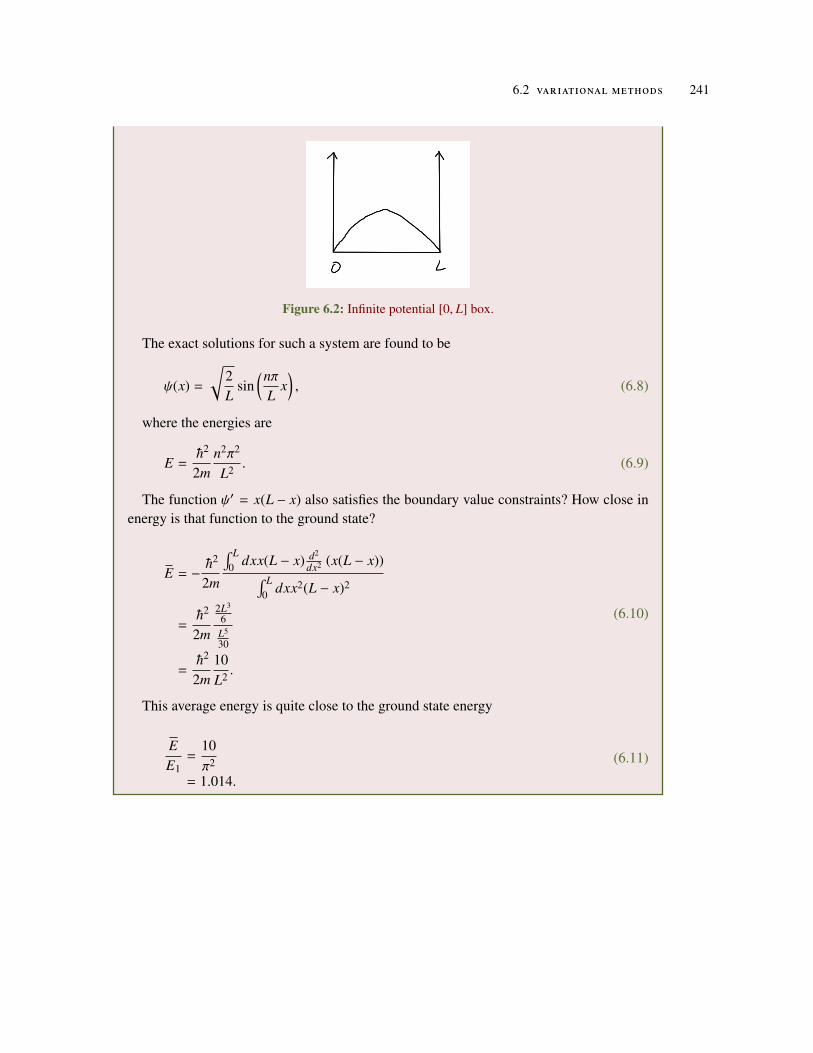
6.2 variational methods 241
Figure 6.2: Infinite potential [0, L] box.
The exact solutions for such a system are found to be
(6.8)ψ(x) =
√2L
sin(nπ
Lx),
where the energies are
(6.9)E =h2
2mn2π2
L2 .
The function ψ′ = x(L − x) also satisfies the boundary value constraints? How close inenergy is that function to the ground state?
(6.10)
E = −h2
2m
∫ L0 dxx(L − x) d2
dx2 (x(L − x))∫ L0 dxx2(L − x)2
=h2
2m
2L3
6L5
30
=h2
2m10L2 .
This average energy is quite close to the ground state energy
(6.11)EE1
=10π2
= 1.014.

242 approximation methods
Example 6.2: Particle in a symmetric box.

6.2 variational methods 243
Figure 6.3: Infinite potential [−L/2, L/2] box.Shifting the boundaries, as sketched in fig. 6.3 doesn’t change the energy levels. For this
potential let’s try a shifted trial function
(6.12)ψ(x) =
(x −
L2
) (x +
L2
)= x2 −
L2
4,
without worrying about the form of the exact solution. This produces the same result asabove
(6.13)
E = −h2
2m
∫ L0 dx
(x2 − L2
4
)d2
dx2
(x2 − L2
4
)∫ L
0 dx(x2 − L2
4
)2
= −h2
2m−2L3/6
L5
30
=h2
2m10L2 .
Summary (Nishant) The above example is that of a particle in a box. The actual wave functionis a sin as shown. But we can come up with a guess wave function that meets the boundaryconditions and ask how accurate it is compared to the actual one.
Basically we are assuming a wave function form and then seeing how it differs from the exactform. We cannot do this if we have nothing to compare it against. But, we note that the varianceof the number operator in the systems eigenstate is zero. So we can still calculate the varianceand try to minimize it. This is one way of coming up with an approximate wave function. Thisdoes not necessarily give the ground state wave function though. For this we need to minimizethe energy itself.

244 approximation methods
6.3 variational method
Today we want to use the variational degree of freedom to try to solve some problems that wedon’t have analytic solutions for.
Anharmonic oscillator
V(x) =12
mω2x2 + λx4, λ ≥ 0. (6.14)
With the potential growing faster than the harmonic oscillator, which had a ground statesolution
(6.15)ψ(x) =1π1/4
1
a1/20
e−x2/2a20 ,
where
(6.16)a0 =
√h
mω.
Let’s try allowing a0 → a, to be a variational degree of freedom
(6.17)ψa(x) =1π1/4
1a1/2 e−x2/2a2
,
(6.18)〈ψa|H |ψa〉 = 〈ψa|p2
2m+
12
mω2x2 + λx4 |ψa〉
We can find
(6.19)⟨x2
⟩=
12
a2
(6.20)⟨x4
⟩=
34
a4
Define
(6.21)ω =h
ma2 ,
so that
(6.22)
Ea = 〈ψa|
(p2
2m+
12
mω2x2)
+
(12
m(ω2 − ω2
)x2 + λx4
)|ψa〉
=12
hω +12
m(ω2 − ω2
) 12
a2 +34λa4.

6.3 variational method 245
Figure 6.4: Energy after perturbation.
Write this as
(6.23)Eω =12
hω +14
hω
(ω2 − ω2
)+
34λ
h2
m2ω2 .
This might look something like fig. 6.4.Demand that
(6.24)
0 =∂Eω
∂ω
=h2−
h4ω2
ω2 −h4
+34
(−2)λ h2
m2ω3
=h4
(1 −
ω2
ω2 − 6λ h
m2ω3
)or
(6.25)ω3 − ω2ω −6λ hm2 = 0.
for λa40 hω, we have something like ω = ω + ε. Expanding eq. (6.25) to first order in ε,
this gives
ω3 + 3ω2ε −ω2 (ω + ε) −6λ hm2 = 0, (6.26)
so that
2ω2ε =6λ hm2 , (6.27)

246 approximation methods
and
hε =3λ h2
m2ω2 = 3λa40. (6.28)
Plugging into
(6.29)
Eω+ε =12
h (ω + ε) +14
hω
(−2ωε + ε2
)+
34λ
h2
m2ω2
≈12
h (ω + ε) −12
hε +34λ
h2
m2ω2
=12
hω +34λa4
0.
With eq. (6.28), that is
Eω=ω+ε ≈12
h(ω +
ε
2
). (6.30)
The energy levels are shifted slightly for each shift in the Hamiltonian frequency.What do we have in the extreme anharmonic limit, where λa4
0 hω. Now we get
ω∗ =
(6 hλm2
)1/3
, (6.31)
and
Eω∗ =h4/3λ1/3
m2/3
38
61/3. (6.32)
(this last result is pulled from a web treatment somewhere of the anharmonic oscillator). Notethat the first factor in this energy, with h4λ/m2 traveling together could have been worked outon dimensional grounds.
This variational method tends to work quite well in these limits. For a system where m = ω =
h = 1, for this problem, we have
Example: (sketch) double well potential
V(x) =mω2
8a2 (x − a)2 (x + a)2. (6.33)
Note that this potential, and the Hamiltonian, both commute with parity.

6.3 variational method 247
Table 6.1: Comparing numeric and variational solutions
h/ω numeric variational
100 3.13 3.16
1000 6.69 6.81
Figure 6.5: Double well potential.
We are interested in the regime where a20 = h
mω a2.Near x = ±a, this will be approximately
V(x) =12
mω2 (x ± a)2. (6.34)
Guessing a wave function that is an eigenstate of parity
Ψ± = g± (φR(x) ± φL(x)) . (6.35)
perhaps looking like the even and odd functions sketched in fig. 6.6, and fig. 6.7.
Figure 6.6: Even double well function.

248 approximation methods
Figure 6.7: Odd double well function.
Using harmonic oscillator functions
φL(x) = ΨH.O.(x + a)
φR(x) = ΨH.O.(x − a)(6.36)
After doing a lot of integral (i.e. in the problem set), we will see a splitting of the variationalenergy levels as sketched in fig. 6.8.
Figure 6.8: Splitting for double well potential.
This sort of level splitting was what was used in the very first mazers.
6.4 perturbation theory (outline)
Given
H = H0 + λV, (6.37)
where λV is “small”. We want to figure out the eigenvalues and eigenstates of this Hamilto-nian
H |n〉 = En |n〉 . (6.38)
We don’t know what these are, but do know that
H0∣∣∣n(0)
⟩= E(0)
n
∣∣∣n(0)⟩. (6.39)

6.5 simplest perturbation example . 249
Figure 6.9: Adiabatic transitions.
We are hoping that the level transitions have adiabatic transitions between the original andperturbed levels as sketched in fig. 6.9.
and not crossed level transitions as sketched in fig. 6.10.
Figure 6.10: Crossed level transitions.
If we have level crossings (which can in general occur), as opposed to adiabatic transitions,then we have no hope of using perturbation theory.
6.5 simplest perturbation example .
Given a 2 × 2 Hamiltonian H = H0 + V , where
(6.40)H =
a c
c∗ b
,note that if c = 0 is
H = H0 =
a 0
0 b
. (6.41)
The off diagonal terms can be considered to be a perturbation
(6.42)V =
0 c
c∗ 0
,with H = H0 + V .

250 approximation methods
Energy levels after perturbation We can solve for the eigenvalues of H easily, finding
(6.43)λ± =a + b
2±
√(a − b
2
)2
+ |c|2.
Plots of a few a, b variations of λ± are shown in fig. 6.11. The quadratic (non-degenerate)domain is found near the c = 0 points of all but the first ( a = b ) plot, and the degenerate (linearin |c|2) regions are visible for larger values of c.
(a) (b)
(c) (d)
Figure 6.11: Plots of λ± for (a, b) ∈ (1, 1), (1, 0), (1, 5), (−8, 8)
Some approximations Suppose that |c| |a − b|, then
(6.44)λ± ≈a + b
2±
∣∣∣∣∣a − b2
∣∣∣∣∣ (1 + 2|c|2
|a − b|2
).
If a > b, then
(6.45)λ± ≈a + b
2±
a − b2
(1 + 2
|c|2
(a − b)2
).

6.6 general non-degenerate perturbation 251
(6.46)
λ+ =a + b
2+
a − b2
(1 + 2
|c|2
(a − b)2
)= a + (a − b)
|c|2
(a − b)2
= a +|c|2
a − b,
and
(6.47)
λ− =a + b
2−
a − b2
(1 + 2
|c|2
(a − b)2
)= b + (a − b)
|c|2
(a − b)2
= b +|c|2
a − b.
This adiabatic evolution displays a “level repulsion”, quadratic in |c|, and is described as anon-degenerate permutation.
If |c| |a − b|, then
(6.48)
λ± =a + b
2± |c|
√1 +
1
|c|2
(a − b
2
)2
≈a + b
2± |c|
1 +1
2|c|2
(a − b
2
)2=
a + b2± |c| ±
(a − b)2
8|c|.
Here we loose the adiabaticity, and have “level repulsion” that is linear in |c|. We no longerhave the sign of a − b in the expansion. This is described as a degenerate permutation.
6.6 general non-degenerate perturbation
Given an unperturbed system with solutions of the form
H0∣∣∣n(0)
⟩= E(0)
n
∣∣∣n(0)⟩, (6.49)
we want to solve the perturbed Hamiltonian equation
(H0 + λV) |n〉 =(E(0)
n + ∆n)|n〉 . (6.50)

252 approximation methods
Here ∆n is an energy shift as that goes to zero as λ→ 0. We can write this as
(E(0)
n − H0)|n〉 = (λV − ∆n) |n〉 . (6.51)
We are hoping to iterate with application of the inverse to an initial estimate of |n〉
|n〉 =(E(0)
n − H0)−1
(λV − ∆n) |n〉 . (6.52)
This gets us into trouble if λ→ 0, which can be fixed by using
|n〉 =(E(0)
n − H0)−1
(λV − ∆n) |n〉 +∣∣∣n(0)
⟩, (6.53)
which can be seen to be a solution to eq. (6.51). We want to ask if
(λV − ∆n) |n〉 , (6.54)
contains a bit of∣∣∣n(0)
⟩? To determine this act with
⟨n(0)
∣∣∣ on the left
(6.55)
⟨n(0)
∣∣∣ (λV − ∆n) |n〉 =⟨n(0)
∣∣∣ (E(0)n − H0
)|n〉
=(E(0)
n − E(0)n
) ⟨n(0)
∣∣∣n⟩= 0.
This shows that |n〉 is entirely orthogonal to∣∣∣n(0)
⟩.
Define a projection operator
(6.56)Pn =∣∣∣n(0)
⟩ ⟨n(0)
∣∣∣ ,which has the idempotent property P2
n = Pn that we expect of a projection operator.Define a rejection operator
(6.57)Pn = 1 −
∣∣∣n(0)⟩ ⟨
n(0)∣∣∣
=∑m,n
∣∣∣m(0)⟩ ⟨
m(0)∣∣∣ .
Because |n〉 has no component in the direction∣∣∣n(0)
⟩, the rejection operator can be inserted
much like we normally do with the identity operator, yielding
(6.58)|n〉 ′ =(E(0)
n − H0)−1
Pn (λV − ∆n) |n〉 +∣∣∣n(0)
⟩,
valid for any initial |n〉.

6.6 general non-degenerate perturbation 253
Power series perturbation expansion Instead of iterating, suppose that the unknown state andunknown energy difference operator can be expanded in a λ power series, say
(6.59)|n〉 = |n0〉 + λ |n1〉 + λ2 |n2〉 + λ3 |n3〉 + · · ·
and(6.60)∆n = ∆n0 + λ∆n1 + λ2∆n2 + λ3∆n3 + · · ·
We usually interpret functions of operators in terms of power series expansions. In the case of(E(0)
n − H0)−1
, we have a concrete interpretation when acting on one of the unperturbed eigen-states
(6.61)1
E(0)n − H0
∣∣∣m(0)⟩
=1
E(0)n − E0
m
∣∣∣m(0)⟩.
This gives
(6.62)|n〉 =1
E(0)n − H0
∑m,n
∣∣∣m(0)⟩ ⟨
m(0)∣∣∣ (λV − ∆n) |n〉 +
∣∣∣n(0)⟩,
or
|n〉 =∣∣∣n(0)
⟩+
∑m,n
∣∣∣m(0)⟩ ⟨
m(0)∣∣∣
E(0)n − E(0)
m
(λV − ∆n) |n〉 . (6.63)
From eq. (6.51), note that
∆n =
⟨n(0)
∣∣∣ λV |n〉⟨n0
∣∣∣n⟩ , (6.64)
however, we will normalize by setting⟨n0
∣∣∣n⟩ = 1, so
∆n =⟨n(0)
∣∣∣ λV |n〉 . (6.65)
to O(λ0) If all λn, n > 0 are zero, then we have
(6.66a)|n0〉 =∣∣∣n(0)
⟩+
∑m,n
∣∣∣m(0)⟩ ⟨
m(0)∣∣∣
E(0)n − E(0)
m
(−∆n0
)|n0〉
(6.66b)∆n0
⟨n(0)
∣∣∣n0⟩
= 0
so
(6.67)|n0〉 =
∣∣∣n(0)⟩
∆n0 = 0.

254 approximation methods
to O(λ1) Requiring identity for all λ1 terms means
(6.68)|n1〉 λ =∑m,n
∣∣∣m(0)⟩ ⟨
m(0)∣∣∣
E(0)n − E(0)
m
(λV − ∆n1λ
)|n0〉 ,
so
(6.69)|n1〉 =∑m,n
∣∣∣m(0)⟩ ⟨
m(0)∣∣∣
E(0)n − E(0)
m
(V − ∆n1
)|n0〉 .
With the assumption that∣∣∣n(0)
⟩is normalized, and with the shorthand
(6.70)Vmn =⟨m(0)
∣∣∣ V ∣∣∣n(0)⟩,
that is
|n1〉 =∑m,n
∣∣∣m(0)⟩
E(0)n − E(0)
m
Vmn
∆n1 =⟨n(0)
∣∣∣ V ∣∣∣n(0)⟩
= Vnn.
(6.71)
to O(λ2) The second order perturbation states are found by selecting only the λ2 contributionsto
(6.72)λ2 |n2〉 =∑m,n
∣∣∣m(0)⟩ ⟨
m(0)∣∣∣
E(0)n − E(0)
m
(λV − (λ∆n1 + λ2∆n2)
)(|n0〉 + λ |n1〉) .
Because |n0〉 =∣∣∣n(0)
⟩, the λ2∆n2 is killed, leaving
(6.73)|n2〉 =
∑m,n
∣∣∣m(0)⟩ ⟨
m(0)∣∣∣
E(0)n − E(0)
m
(V − ∆n1
)|n1〉
=∑m,n
∣∣∣m(0)⟩ ⟨
m(0)∣∣∣
E(0)n − E(0)
m
(V − ∆n1
)∑l,n
∣∣∣l(0)⟩
E(0)n − E(0)
l
Vln,
which can be written as
(6.74)|n2〉 =∑
l,m,n
∣∣∣m(0)⟩ VmlVln(
E(0)n − E(0)
m
) (E(0)
n − E(0)l
) −∑m,n
∣∣∣m(0)⟩ VnnVmn(
E(0)n − E(0)
m
)2 .
For the second energy perturbation we have
6.7 stark effect 255
(6.75)λ2∆n2 =⟨n(0)
∣∣∣ λV (λ |n1〉) ,
or
(6.76)
∆n2 =⟨n(0)
∣∣∣ V |n1〉
=⟨n(0)
∣∣∣ V ∑m,n
∣∣∣m(0)⟩
E(0)n − E(0)
m
Vmn.
That is
(6.77)∆n2 =∑m,n
VnmVmn
E(0)n − E(0)
m
.
to O(λ3) Similarly, it can be shown that
(6.78)∆n3 =∑
l,m,n
VnmVmlVln(E(0)
n − E(0)m
) (E(0)
n − E(0)l
) −∑m,n
VnmVnnVmn(E(0)
n − E(0)m
)2 .
In general, the energy perturbation is given by
(6.79)∆(l)n =
⟨n(0)
∣∣∣ V |nl−1〉 .
6.7 stark effect
(6.80)H = Hatom + eEz,
where Hatom is assumed to be Hydrogen-like with Hamiltonian
(6.81)Hatom =p2
2m−
e2
4πε0r,
and wave functions
(6.82)〈r|ψnlm〉 = Rnl(r)Ylm(θ, φ)
Referring to eq. (A.117), the first level correction to the energy
(6.83)∆1 = 〈ψ100| eEz |ψ100〉
= eE∫
dΩ4π
cos θ∫
drr2R2100(r)
The cosine integral is obliterated, so we have ∆1 = 0.

256 approximation methods
How about the second order energy correction? That is
(6.84)∆2 =∑
nlm,100
|〈ψ100| eEz |nlm〉|2
E(0)100 − Enlm
The matrix element in the numerator is the absolute square of
(6.85)V100,nlm = eE∫
dΩ1√
4πcos θYlm(θ, φ)
∫drr3R100(r)Rnl(r).
For all m , 0, Ylm includes a eimφ factor, so this cosine integral is zero. For m = 0, each of theYlm functions appears to contain either even or odd powers of cosines (see: eq. (A.115)). Thisshows that for even 2k = l, the cosine integral is zero
∫ π
0sin θ cos θ
∑k
ak cos2k θdθ = 0, (6.86)
since cos2k(θ) is even and sin θ cos θ is odd over the same interval. We find zero for∫ π
0 sin θ cos θY30(θ, φ)dθ,and Mathematica appears to show that the rest of these integrals for l > 1 are also zero.
FIXME: find the property of the spherical harmonics that can be used to prove that this istrue in general for l > 1.
This leaves
(6.87)∆2 =
∑n,1
|〈ψ100| eEz |n10〉|2
E(0)100 − En10
= −e2E2∑n,1
|〈ψ100| z |n10〉|2
En10 − E(0)100
.
This is sometimes written in terms of a polarizability α
(6.88)∆2 = −E2
2α,
where
(6.89)α = 2e2∑n,1
|〈ψ100| z |n10〉|2
En10 − E(0)100
.
With
P = αE, (6.90)

6.7 stark effect 257
the energy change upon turning on the electric field from 0→ E is simply −P · dE integratedfrom 0→ E. Putting P = αEz, we have
(6.91)−
∫ E
0PzdE = −
∫ E
0αEdE
= −12αE2
leading to an energy change −αE2/2, so we can directly compute 〈P〉 or we can computechange in energy, and both contain information about the polarization factor α.
There is an exact answer to the sum eq. (6.89), but we aren’t going to try to get it here. Insteadlet’s look for bounds
∆min2 < ∆2 < ∆max
2 (6.92)
(6.93)αmin = 2e2 |〈ψ100| z |ψ210〉|2
E(0)210 − E(0)
100
For the hydrogen atom we have
(6.94)En = −e2
2n2a0,
allowing any difference of energy levels to be expressed as a fraction of the ground stateenergy, such as
(6.95)E(0)
210 =14
E(0)100
=14− h2
2ma20
So
(6.96)E(0)210 − E(0)
100 =34
h2
2ma20
In the numerator we have

258 approximation methods
(6.97)
〈ψ100| z |ψ210〉 =
∫r2dΩ
1√πa3/2
0
e−r/a0
r cos θ
1
4√
2πa3/20
ra0
e−r/2a0 cos θ
= (2π)
1√π
1
4√
2πa0
∫ π
0dθ sin θ cos2 θ
∫ ∞
0
dra0
r4
a40
e−r/a0−r/2a0
= (2π)1√π
1
4√
2πa0
−u3
3
∣∣∣∣∣∣−1
1
∫ ∞
0s4dse−3s/2
=1
2√
2
23
a025681
=1
3√
2
25681
a0
≈ 0.75a0.
This gives
(6.98)
αmin =2e2(0.75)2a2
034
h2
2ma20
=64
2me2a40
h2
= 3me2a4
0
h2
= 34πε0
a0a4
0
≈ 4πε0a30 × 3.
The factor 4πε0a30 are the natural units for the polarizability.
There is a neat trick that generalizes to many problems to find the upper bound. Recall thatthe general polarizability was
(6.99)α = 2e2∑
nlm,100
|〈100| z |nlm〉|2
Enlm − E(0)100
.
If we are looking for the upper bound, and replace the denominator by the smallest energydifference that will be encountered, it can be brought out of the sum, for
(6.100)αmax = 2e2 1
E210 − E(0)100
∑nlm,100
〈100| z |nlm〉 〈nlm| z |100〉

6.7 stark effect 259
Because 〈nlm| z |100〉 = 0, the constraint in the sum can be removed, and the identity summa-tion evaluated
(6.101)
αmax = 2e2 1
E210 − E(0)100
∑nlm
〈100| z |nlm〉 〈nlm| z |100〉
=2e2
34
h2
2ma20
〈100| z2 |100〉
=16e2ma2
0
3 h2 × a20
= 4πε0a30 ×
163.
The bounds are
3 ≥α
αat <163, (6.102)
where
(6.103)αat = 4πε0a30.
The actual value is
(6.104)α
αat =92.
See lecture21someSphericalHarmonicsAndTheirIntegrals.nb, for some of the integrals above,and for spherical harmonic tables.
Example: Computing the dipole moment
〈Pz〉 = αE = 〈ψ100| ez |ψ100〉 . (6.105)
Without any perturbation this is zero. After perturbation, retaining only the terms that are firstorder in δψ100 we have
(6.106)〈ψ100 + δψ100| ez |ψ100 + δψ100〉 ≈ 〈ψ100| ez |δψ100〉 + 〈δψ100| ez |ψ100〉 .
Next time: van der Walls We will look at two hyrdogenic atomic systems interacting wherethe pair of nuclei are supposed to be infinitely heavy and stationary. The wave functions each setof atoms are individually known, but we can consider the problem of the interactions of atom1’s electrons with atom 2’s nucleus and atom 2’s electrons, and also the opposite interactions ofatom 2’s electrons with atom 1’s nucleus and its electrons. This leads to a result that is linear inthe electric field (unlike the above result, which is called the quadratic Stark effect).

260 approximation methods
Another approach (for last time?) Imagine we perturb a potential, say a harmonic oscillatorwith an electric field
(6.107)V0(x) =12
kx2
(6.108)V(x) = Eex
After minimizing the energy, using ∂V/∂x = 0, we get
(6.109)12
kx2 + Eex→ kx∗
= −eE
(6.110)p∗ = −ex∗
= −e2E
k
For such a system the polarizability is
(6.111)α =e2
k
(6.112)
12
k(−
eEk
)2
+ Ee(−
eEk
)= −
12
(e2
k
)E2
= −12αE2
6.8 van der walls potential
(6.113)H0 = H01 + H02,
where
H0α =p2α
2m−
e2
4πε0|rα −Rα|, α = 1, 2 (6.114)
The full interaction potential is
(6.115)V =e2
4πε0
(1
|R1 − R2|+
1|r1 − r2|
−1
|r1 − R2|−
1|r2 − R1|
)

6.8 van der walls potential 261
Figure 6.12: Two atom interaction.
Let
(6.116)xα = rα − Rα,
(6.117)R = R1 − R2,
as sketched in fig. 6.12.
(6.118)H0α =p2
2m−
e2
4πε0|xα|
which allows the total interaction potential to be written
(6.119)V =e2
4πε0R
(1 +
R|x1 − x2 + R|
−R
|x1 + R|−
R|−x2 + R|
)For R x1, x2, this interaction potential, after a multipole expansion, is approximately
(6.120)V =e2
4πε0
(x1 · x2
|R|3− 3
(x1 · R)(x2 · R)
|R|5
)Showing this is left as a exercise.
1. O(λ) .With
(6.121)ψ0 = |1s, 1s〉
(6.122)∆E(1) = 〈ψ0|V |ψ0〉
The two particle wave functions are of the form
(6.123)〈x1, x2|ψ0〉 = ψ1s(x1)ψ1s(x2),

262 approximation methods
so braket integrals must be evaluated over a six-fold space. Recall that
(6.124)ψ1s =1
√πa3/2
0
e−r/a0 ,
so
(6.125)〈ψ1s| xi |ψ1s〉 ∝
∫ π
0sin θdθ
∫ 2π
0dφxi
where(6.126)xi ∈ r sin θ cos φ, r sin θ sin φ, r cos θ .
The x, y integrals are zero because of the φ integral, and the z integral is proportional to∫ π
0 sin(2θ)dθ, which is also zero. This leads to zero averages
〈x1〉 = 0 = 〈x2〉 (6.127)
so
(6.128)∆E(1) = 0.
2. O(λ2) .
(6.129)∆E(2) =
∑n,0
|〈ψn|V |ψ0〉|2
E0 − En
=∑n,0
〈ψ0|V |ψn〉 〈ψn|V |ψ0〉
E0 − En.
This is a sum over all excited states.We expect that this will be of the form
(6.130)∆E(2) = −
(e2
4πε0
)2 C6
R6
x1 and x2 are dipole operators. The first time this has a non-zero expectation is when we gofrom the 1s to the 2p states (both 1s and 2s states are spherically symmetric).
Noting that En = −e2/2n2a0, we can compute a minimum bound for the energy denominator
(6.131)
(En − E0)min = 2(E2p − E1s
)= 2E1s
(14− 1
)= 2
34|E1s|
=32|E1s|.

6.8 van der walls potential 263
Note that the factor of two above comes from summing over the energies for both electrons.This gives us
(6.132)C6 =32|E1s| 〈ψ0| V |ψ0〉 ,
where
(6.133)V =(x1 · x2 − 3(x1 · R)(x2 · R)
)What about degeneracy?
(6.134)∆E(2)n =
∑m,n
|〈ψn|V |ψ0〉|2
E0 − En
If 〈ψn|V |ψm〉 ∝ δnm then it’s okay. In general the we can’t expect the matrix element will beanything but fully populated, say
(6.135)V =
V11 V12 V13 V14
V21 V22 V23 V24
V31 V32 V33 V34
V41 V42 V43 V44
,
If we choose a basis so that
(6.136)V =
V11
V22
V33
V44
.
When this is the case, we have no mixing of elements in the sum of eq. (6.134)
Degeneracy in the Stark effect
(6.137)H = H0 + eEz,
where
(6.138)H0 =p2
2m−
e4πε0
1|x|
Consider the states 2s, 2px, 2py, 2pz, for which E(0)n ≡ E2s, as sketched in fig. 6.13.

264 approximation methods
Figure 6.13: 2s 2p degeneracy.
Because of spherical symmetry
〈2s| eEz |2s〉 = 0
〈2px| eEz |2px〉 = 0⟨2py
∣∣∣ eEz∣∣∣2py
⟩= 0
〈2pz| eEz |2pz〉 = 0
(6.139)
Looking at odd and even properties, it turns out that the only off-diagonal matrix element is
〈2s| eEz |2pz〉 = V1 = −3eEa0. (6.140)
With a2s, 2px, 2py, 2pz
basis the potential matrix is
(6.141)
0 0 0 V1
0 0 0 0
0 0 0 0
V∗1 0 0 0
(6.142)
0 −|V1|
−|V1| 0
implies that the energy splitting goes as
E2s → E2s ± |V1|, (6.143)
as sketched in fig. 6.14.

6.9 problems 265
Figure 6.14: Stark effect energy level splitting.
The diagonalizing states corresponding to eigenvalues ±3a0E, are (|2s〉 ∓ |2pz〉)/√
2.The matrix element above is calculated explicitly in lecture22Integrals.nb.The degeneracy that is left unsplit here, and has to be accounted for should we attempt higher
order perturbation calculations.
6.9 problems
Exercise 6.1 van der Walls multipole expansion.
Prove eq. (6.120).Answer for Exercise 6.1
Noting that
(6.144)(1 + ε)−1/2 = 1 −12ε −
12
(−32
)12!ε2 = 1 −
12ε +
38ε2,
we have
(6.145)
R|ε + R|
=1∣∣∣ εR + R
∣∣∣=
(1 + 2
ε
R· R +
( εR
)2)−1/2
= 1 −ε
R· R −
12
( εR
)2+
38
(2ε
R· R +
( εR
)2)2
= 1 −ε
R· R −
12
( εR
)2+
38
(4( εR· R
)2+
( εR
)4+ 4
ε
R· R
( εR
)2)
≈ 1 −ε
R· R −
12
( εR
)2+
32
( εR· R
)2.

266 approximation methods
Inserting the values from the brackets of eq. (6.119) we have
(6.146)
1 +R
|x1 − x2 + R|−
R|x1 + R|
−R
|−x2 + R|
= −(x1 − x2)
R· R −
12
((x1 − x2)
R
)2
+32
((x1 − x2)
R· R
)2
+x1
R· R +
12
(x1
R
)2−
32
(x1
R· R
)2
−x2
R· R +
12
(x2
R
)2−
32
(x2
R· R
)2
=x1
R·
x2
R+
32
((x1 − x2)
R· R
)2
−32
(x1
R· R
)2
−32
(x2
R· R
)2
=x1
R·
x2
R− 3
x1
R· R
x2
R· R.
This proves eq. (6.120).
Exercise 6.2 Harmonic oscillator with energy shift. ([11] pr. 5.1)
Given a perturbed 1D SHO Hamiltonian
(6.147)H =1
2mp2 +
12
mω2x2 + λbx,
calculate the first non-zero perturbation to the ground state energy. Then solve for that energydirectly and compare.Answer for Exercise 6.2
The first order energy shift is seen to be zero
(6.148)
∆(0)0 = V00
= 〈0| bx |0〉
=x0√
2〈0| a + a† |0〉
=x0√
2〈0|1〉
= 0.
The first order perturbation to the ground state is

6.9 problems 267
(6.149)
∣∣∣0(1)⟩
=∑m,0
|m〉 〈m| bx |0〉hω/2 − hω(m − 1/2)
= −bx0√
2 hω
∑m,0
|m〉 〈m|1〉m
= −bx0√
2 hω|1〉 .
The second order ground state energy perturbation is
(6.150)
∆(2)0 = 〈0| bx
∣∣∣0(1)⟩
=bx0√
2〈0| a + a†
(−b
x0√
2 hω|1〉
)=
bx0√
2
(−b
x0√
2 hω
)= −
b2x20
2 hω
= −b2
2 hωh
mω
= −b2
2mω2 ,
so the total energy perturbation up to second order is
(6.151)∆0 = −λ2 b2
2mω2 .
To compare to the exact result, rewrite the Hamiltonian as
(6.152)H =
12m
p2 +12
mω2(x2 +
2λbxmω2
)=
12m
p2 +12
mω2(x +
λbmω2
)2
−12
mω2(λb
mω2
)2
.
The Hamiltonian is subject to a constant energy shift
(6.153)∆E = −
12
mω2 λ2b2
m2ω4
= −λ2b2
2mω2 .
This is an exact match with the second order perturbation result of eq. (6.151).

268 approximation methods
Exercise 6.3 Double well potential. (2015 ps7 p1)Consider a particle in the double well potential
(6.154)V(x) =mω2
8a2 (x + a)2 (x − a)2 .
Expanding V(x) around x = ±a leads to a harmonic potential with frequency ω. Constructvariational states with even/odd parity as ψ±(x) = g± (φ(x − a) ± φ(x + a)) where φ(x) is thenormalized ground state of the usual harmonic oscillator with frequency ω, i.e.,
φ(x) =
1πa2
0
1/4
e− x2
2a20 ; a0 =
√h
mω. (6.155)
a. Determine the normalization constants g±. Next using these wavefunctions, determinethe variational energies of these two states. Hence determine the ‘tunnel splitting’ be-tween the two states, induced by the tunneling through the barrier region. In your cal-culations, you can assume a a0, so retain only the leading terms in any polynomialsyou might encounter when you do the integrals.
b. If we pay attention to these lowest two states (left well and right well) in the full Hilbertspace, we can write a phenomenological 2 × 2 Hamiltonian
(6.156)H =
ε0 −γ
−γ ε0
,where ε0 is the energy on each side, and γ leads to tunneling, so if we start off in theleft well, t leads to a nonzero amplitude to find it in the right well at a later time. Findits eigenvalues and eigenvectors. Comparing with your variational result for the energysplitting, determine the ‘tunnel coupling’ γ.
Answer for Exercise 6.3PROBLEM SET RELATED MATERIAL REDACTED IN THIS DOCUMENT.PLEASE
FEEL FREE TO EMAIL ME FOR THE FULL VERSION IF YOU AREN’T TAKING PHY1520.. .
. ..
. . .. .
. . .. .
. .. END-REDACTION

6.9 problems 269
Exercise 6.4 Helium-4 atom. (2015 ps7 p2)
Consider the Helium atom with atomic number Z = 2, which leads to the nuclear chargeZ = 2e, and two electrons with charge −e each.
a. Show that ignoring electron-electron interactions leads to a ground state energy EHe =
4EH where EH is the ground state energy of the hydrogen atom.
b. Consider the full problem which retains the Coulomb interaction between the electrons,i.e.
(6.157)H =1
2m
(p2
1 + p22
)− 2e2 1
4πε0
(1r1
+1r2
)+ e2 1
4πε0
1|r1 − r2|
.
and consider the variational wavefunction
(6.158)ψ(r1, r2) = Ne−1a (r1+r2).
where N is the normalization constant, and a is a variational parameter. Determine thevariational ground state energy, and minimize with respect to a to find the best estimatefor the ground state energy of Helium. Compare with numerical estimates of the energy.
Answer for Exercise 6.4PROBLEM SET RELATED MATERIAL REDACTED IN THIS DOCUMENT.PLEASE
FEEL FREE TO EMAIL ME FOR THE FULL VERSION IF YOU AREN’T TAKING PHY1520.. .
. ..
. . .. .
. . .. .
. .. END-REDACTION
Exercise 6.5 Harmonic oscillator variation. ([2] pr. 24.3)
Consider a 1D harmonic oscillator with an unnormalized trial wavefunction ψv(x) = e−β|x|.Minimize the ground state energy with respect to β, thus obtaining the optimal β as well as thevariational ground state energy. Compare with the exact result. Note that you need to be carefulevaluating derivatives since the wavefunction has a ‘cusp’ at x = 0.Answer for Exercise 6.5
PROBLEM SET RELATED MATERIAL REDACTED IN THIS DOCUMENT.PLEASEFEEL FREE TO EMAIL ME FOR THE FULL VERSION IF YOU AREN’T TAKING PHY1520.

270 approximation methods
. .. .
.. . .
. .. . .
. .. .
. END-REDACTION
Exercise 6.6 Energy estimate for an absolute value potential. ([11] pr. 5.21)Estimate the lowest eigenvalue λ of the differential equation
(6.159)d2
dx2ψ + (λ − |x|)ψ = 0.
Using α variation with the trial function
(6.160)ψ =
c(α − |x|) |x| < α
0 |x| > α
Answer for Exercise 6.6First rewrite the differential equation in a Hamiltonian like fashion
Hψ = −d2
dx2ψ + |x|ψ = λψ. (6.161)
We need the derivatives of the trial distribution. The first derivative is
(6.162)
ddxψ = −c
ddx|x|
= −cddx
(xθ(x) − xθ(−x))
= −c (θ(x) − θ(−x) + xδ(x) + xδ(−x))= −c (θ(x) − θ(−x) + 2xδ(x)) .
The second derivative is
(6.163)
d2
dx2ψ = −cddx
(θ(x) − θ(−x) + 2xδ(x))
= −c(δ(x) + δ(−x) + 2δ(x) + 2xδ′(x)
)= −c
(4δ(x) + 2x
−δ(x)x
)= −2cδ(x).

6.9 problems 271
This gives
(6.164)Hψ = −2cδ(x) + |x|c (α − |x|) .
We are now set to compute some of the inner products. The normalization is the simplest
(6.165)
〈ψ|ψ〉 = c2∫ α
−α(α − |x|)2dx
= 2c2∫ α
0(x − α)2dx
= 2c2∫ 0
−αu2du
= 2c2(−
(−α)3
3
)=
23
c2α3.
For the energy
(6.166)
〈ψ|Hψ〉 = c2∫
dx (α − |x|) (−2δ(x) + |x| (α − |x|))
= c2(−2α +
∫ α
−αdx (α − |x|)2
|x|)
= c2(−2α + 2
∫ 0
−αduu2 (u + α)
)= c2
−2α + 2(u4
4+ α
u3
3
)∣∣∣∣∣∣0−α
= c2
(−2α − 2
(α4
4−α4
3
))= c2
(−2α +
16α4
).
The energy estimate is
(6.167)
E =〈ψ|Hψ〉〈ψ|ψ〉
=−2α + 1
6α4
23α
3
= −3α2 +
14α.
272 approximation methods
This has its minimum at
(6.168)0 = −6α3 +
14,
or
(6.169)α = 2 × 31/3.
Back substitution into the energy gives
(6.170)E = −
34 × 32/3 +
12
31/3
=34/3
4≈ 1.08.
The problem says the exact answer is 1.019, so the variation gets within 6 %.
Exercise 6.7 Anharmonic oscillator. (2015 ps8 p1)
Consider a quantum particle in the ground state of a 1D anharmonic oscillator potential
(6.171)V(x) =12
mω2x2 + λx4
= V0 + λV ′.
Compute the first and second order energy shift of this oscillator perturbatively in λ.Answer for Exercise 6.7
PROBLEM SET RELATED MATERIAL REDACTED IN THIS DOCUMENT.PLEASEFEEL FREE TO EMAIL ME FOR THE FULL VERSION IF YOU AREN’T TAKING PHY1520.
. .. .
.. . .
. .. . .
. .. .
. END-REDACTION
Exercise 6.8 Quadrupolar potential. (2015 ps8 p2)

6.9 problems 273
Consider a p-orbital electron of hydrogen with |n, l = 1,m〉, with m = 0,±1, subject to anexternal potential
(6.172)V(x, y, z) = λ(x2 − y2),
with λ being a constant. For fixed n, obtain the correct eigenstates which diagonalize theperturbation, without worrying about doing radial integrals explicitly. Show that the three-folddegeneracy of the p-orbital is completely broken by the perturbation to linear order in λ.Answer for Exercise 6.8
PROBLEM SET RELATED MATERIAL REDACTED IN THIS DOCUMENT.PLEASEFEEL FREE TO EMAIL ME FOR THE FULL VERSION IF YOU AREN’T TAKING PHY1520.
. .. .
.. . .
. .. . .
. .. .
. END-REDACTION
Exercise 6.9 Harmonic oscillator. (2015 ps8 p3)
Consider a 2D harmonic oscillator with
(6.173)H =p2
x
2m+
p2y
2m+
12
mω2(x2 + y2
)Turn on an anharmonic perturbation
(6.174)V = λg1m2ω3
h
(x4 + y4
)+ λ2g2mω2xy,
Note that the potentials have been altered from the original problem statement to have dimen-sions of energy with dimensionless scale factors g1, g2, λ.
a. Derive the equations for the energy shifts and perturbed states for a second order per-turbing potential of the form above.
b. Find the perturbed eigenstate and the corresponding energy shifts up to O(λ2) for theground state. Ignore terms of O(λ3).
c. Do the same for the first two degenerate states.

274 approximation methods
Answer for Exercise 6.9PROBLEM SET RELATED MATERIAL REDACTED IN THIS DOCUMENT.PLEASE
FEEL FREE TO EMAIL ME FOR THE FULL VERSION IF YOU AREN’T TAKING PHY1520.. .
. ..
. . .. .
. . .. .
. .. END-REDACTION
Exercise 6.10 Hyperfine levels. (2015 ps8 p4)
We can schematically model the hyperfine interaction between the electron and proton spinsas ASe · Sp where A is the hyperfine interaction energy.
a. Consider the spin-1/2 proton interacting with a spin-1/2 electron. What are the spineigenstates and eigenvalues?
b. Now consider applying a magnetic field which leads to an extra term
(6.175)−B(geµeS z
e + gpµpS zp
)with gyromagnetic ratios ge ≈ −2 and gp ≈ 5.5, with magnetic moments µe = e/2me
and µp = e/2mp. The large nuclear mass ensures µe/µp ∼ 2000, so let us simply setµp = 0. For convenience, set Bgeµe → Beff so the Hamiltonian becomes
(6.176)H = ASe · Sp − BeffS ze,
so the only dimensionless parameter is Beff/A.Using perturbation theory (degenerate or non-degenerate as appropriate) find how thecoupled hyperfine levels split for weak field Beff/A 1. Also consider the strong fieldlimit Beff/A 1.
c. Compute the full field evolution of the levels and compare with the perturbative lowfield regime result and the high field regime result.
Answer for Exercise 6.10PROBLEM SET RELATED MATERIAL REDACTED IN THIS DOCUMENT.PLEASE
FEEL FREE TO EMAIL ME FOR THE FULL VERSION IF YOU AREN’T TAKING PHY1520.. .
. .

6.9 problems 275
.. . .
. .. . .
. .. .
. END-REDACTION
Exercise 6.11 2D SHO xy perturbation. ([11] pr. 5.4)
Given a 2D SHO with Hamiltonian
(6.177)H0 =1
2m
(p2
x + p2y
)+
mω2
2
(x2 + y2
),
a. What are the energies and degeneracies of the three lowest states?
b. With perturbation
(6.178)V = mω2xy,
calculate the first order energy perturbations and the zeroth order perturbed states.
c. Solve the H0 + δV problem exactly, and compare.
Answer for Exercise 6.11
Part a. Recall that we have
(6.179)H |n1, n2〉 = hω (n1 + n2 + 1) |n1, n2〉 ,
So the three lowest energy states are |0, 0〉 , |1, 0〉 , |0, 1〉 with energies hω, 2 hω, 2 hω respec-tively (with a two fold degeneracy for the second two energy eigenkets).
Part b. Consider the action of xy on the β = |0, 0〉 , |1, 0〉 , |0, 1〉 subspace. Those are
(6.180)
xy |0, 0〉 =x2
0
2
(a + a†
) (b + b†
)|0, 0〉
=x2
0
2
(b + b†
)|1, 0〉
=x2
0
2|1, 1〉 .

276 approximation methods
(6.181)
xy |1, 0〉 =x2
0
2
(a + a†
) (b + b†
)|1, 0〉
=x2
0
2
(a + a†
)|1, 1〉
=x2
0
2
(|0, 1〉 +
√2 |2, 1〉
).
(6.182)
xy |0, 1〉 =x2
0
2
(a + a†
) (b + b†
)|0, 1〉
=x2
0
2
(b + b†
)|1, 1〉
=x2
0
2
(|1, 0〉 +
√2 |1, 2〉
).
The matrix representation of mω2xy with respect to the subspace spanned by basis β above is
(6.183)xy ∼12
hω
0 0 0
0 0 1
0 1 0
.This diagonalizes with
(6.184a)U =
1 0
0 U
(6.184b)U =
1√
2
1 1
1 −1
(6.184c)D =12
hω
0 0 0
0 1 0
0 0 −1
xy = UDU† = UDU. (6.184d)
The unperturbed Hamiltonian in the original basis is
(6.185)H0 = hω
1 0
0 2I
,

6.9 problems 277
So the transformation to the diagonal xy basis leaves the initial Hamiltonian unaltered
(6.186)
H′0 = U†H0U
= hω
1 0
0 U2IU
= hω
1 0
0 2I
.Now we can compute the first order energy shifts almost by inspection. Writing the new basis
as β′ = |0〉 , |1〉 , |2〉 those energy shifts are just the diagonal elements from the xy operatorsmatrix representation
(6.187)
E(1)0 = 〈0|V |0〉 = 0
E(1)1 = 〈1|V |1〉 =
12
hω
E(1)2 = 〈2|V |2〉 = −
12
hω.
The new energies are
(6.188)
E0 → hω
E1 → hω (2 + δ/2)
E2 → hω (2 − δ/2) .
Part c. For the exact solution, it’s possible to rotate the coordinate system in a way that killsthe explicit xy term of the perturbation. That we could do this for x, y operators wasn’t obviousto me, but after doing so (and rotating the momentum operators the same way) the new operatorsstill have the required commutators. Let
(6.189)
uv =
cos θ sin θ
− sin θ cos θ
x
y
=
x cos θ + y sin θ
−x sin θ + y cos θ
.Similarly, for the momentum operators, let
(6.190)
pu
pv
=
cos θ sin θ
− sin θ cos θ
px
py
=
px cos θ + py sin θ
−px sin θ + py cos θ
.
278 approximation methods
For the commutators of the new operators we have
(6.191)
[u, pu
]=
[x cos θ + y sin θ, px cos θ + py sin θ
]=
[x, px
]cos2 θ +
[y, py
]sin2 θ
= i h(cos2 θ + sin2 θ
)= i h.
(6.192)
[v, pv
]=
[−x sin θ + y cos θ,−px sin θ + py cos θ
]=
[x, px
]sin2 θ +
[y, py
]cos2 θ
= i h.
(6.193)
[u, pv
]=
[x cos θ + y sin θ,−px sin θ + py cos θ
]= cos θ sin θ
(−
[x, px
]+
[y, pp
])= 0.
(6.194)
[v, pu
]=
[−x sin θ + y cos θ, px cos θ + py sin θ
]= cos θ sin θ
(−
[x, px
]+
[y, pp
])= 0.
We see that the new operators are canonical conjugate as required. For this problem, we justwant a 45 degree rotation, with
x =1√
2(u + v)
y =1√
2(u − v) .
(6.195)
We have
(6.196)
x2 + y2 =12
((u + v)2 + (u − v)2
)=
12
(2u2 + 2v2 + 2uv − 2uv
)= u2 + v2,

6.9 problems 279
(6.197)
p2x + p2
y =12
((pu + pv)2 + (pu − pv)2
)=
12
(2p2
u + 2p2v + 2pu pv − 2pu pv
)= p2
u + p2v ,
and
(6.198)xy =
12
((u + v)(u − v))
=12
(u2 − v2
).
The perturbed Hamiltonian is
(6.199)H0 + δV =
12m
(p2
u + p2v
)+
12
mω2(u2 + v2 + δu2 − δv2
)=
12m
(p2
u + p2v
)+
12
mω2(u2(1 + δ) + v2(1 − δ)
).
In this coordinate system, the corresponding eigensystem is
(6.200)H |n1, n2〉 = hω(1 + n1
√1 + δ + n2
√1 − δ
)|n1, n2〉 .
For small δ
(6.201)n1√
1 + δ + n2√
1 − δ ≈ n1 + n2 +12
n1δ −12
n2δ,
so
(6.202)H |n1, n2〉 ≈ hω(1 + n1 + n2 +
12
n1δ −12
n2δ
)|n1, n2〉 .
The lowest order perturbed energy levels are
(6.203)|0, 0〉 → hω
(6.204)|1, 0〉 → hω(2 +
12δ
)
(6.205)|0, 1〉 → hω(2 −
12δ
)The degeneracy of the |0, 1〉 , |1, 0〉 states has been split, and to first order match the zeroth
order perturbation result.

280 approximation methods
Exercise 6.12 Perturbation of two state Hamiltonian. ([11] pr. 5.11)
Given a two-state system
(6.206)
H = H0 + λV
=
E1 λ∆
λ∆ E2
a. Solve the system exactly.
b. Find the first order perturbed states and second order energy shifts, and compare to theexact solution.
c. Solve the degenerate case for E1 = E2, and compare to the exact solution.
Answer for Exercise 6.12
Part a. The energy eigenvalues ε are given by
(6.207)0 = (E1 − ε) (E2 − ε) − (λ∆)2,
or
(6.208)ε2 − ε (E1 + E2) + E1E2 = (λ∆)2.
After rearranging this is
(6.209)ε =E1 + E2
2±
√(E1 − E2
2
)2+ (λ∆)2.
Notice that for E2 = E1 we have
(6.210)ε = E1 ± λ∆.
Since a change of basis can always put the problem in a form so that E1 > E2, let’s assumethat to make an approximation of the energy eigenvalues for |λ∆| (E1 − E2)/2
(6.211)
ε =E1 + E2
2±
E1 − E2
2
√1 +
(2λ∆)2
(E1 − E2)2
≈E1 + E2
2±
E1 − E2
2
(1 + 2
(λ∆)2
(E1 − E2)2
)=
E1 + E2
2±
E1 − E2
2±
(λ∆)2
E1 − E2
= E1 +(λ∆)2
E1 − E2, E2 +
(λ∆)2
E2 − E1.
6.9 problems 281
For the perturbed states, starting with the plus case, if
(6.212)|+〉 ∝
ab ,
we must have
(6.213)0 = (E1 −
(E1 +
(λ∆)2
E1 − E2
))a + λ∆b
= (−(λ∆)2
E1 − E2)a + λ∆b,
so
(6.214)|+〉 →
1λ∆
E1−E2
= |+〉 +
λ∆E1 − E2
|−〉 .
Similarly for the minus case we must have
(6.215)0 = λ∆a + (E2 −
(E2 +
(λ∆)2
E2 − E1
))b
= λ∆b + (−(λ∆)2
E2 − E1)b,
for
(6.216)|−〉 → |−〉 +λ∆
E2 − E1|+〉 .
Part b. For the perturbation the first energy shift for perturbation of the |+〉 state is
(6.217)
E(1)+ = |+〉V |+〉
= λ∆[1 0
] 0 1
1 0
10
= λ∆
[1 0
] 01
= 0.

282 approximation methods
The first order energy shift for the perturbation of the |−〉 state is also zero. The perturbed |+〉state is
(6.218)|+〉(1) =
P+
E1 − H0V |+〉
=|−〉 〈−|
E1 − E2V |+〉
The numerator matrix element is
(6.219)
〈−|V |+〉 =[0 1
] 0 ∆
∆ 0
10
=
[0 1
] 0
∆
= ∆,
so
(6.220)|+〉 → |+〉 + |−〉∆
E1 − E2.
Observe that this matches the first order series expansion of the exact value above.For the perturbation of |−〉 we need the matrix element
(6.221)
〈+|V |−〉 =[1 0
] 0 ∆
∆ 0
01
=
[1 0
] ∆0
= ∆,
so it’s clear that the perturbed ket is
(6.222)|−〉 → |−〉 + |+〉∆
E2 − E1,
also matching the approximation found from the exact computation. The second order energyshifts can now be calculated

6.9 problems 283
(6.223)
〈+|V |+〉 ′ =[1 0
] 0 ∆
∆ 0
1
∆E1−E2
=
[1 0
] ∆2
E1−E2
∆
=
∆2
E1 − E2,
and
(6.224)
〈−|V |−〉 ′ =[0 1
] 0 ∆
∆ 0
∆
E2−E1
1
=
[0 1
] ∆∆2
E2−E1
=
∆2
E2 − E1,
The energy perturbations are therefore
(6.225)E1 → E1 +
(λ∆)2
E1 − E2
E2 → E2 +(λ∆)2
E2 − E1.
This is what we had by approximating the exact case.
Part c. For the E2 = E1 case, we’ll have to diagonalize the perturbation potential. That is
(6.226)
V = U∧
U†∧=
∆ 0
0 −∆
U = U† =
1√
2
1 1
1 −1
.A change of basis for the Hamiltonian is

284 approximation methods
(6.227)
H′ = U†HU= U†H0U + λU†VU= E1U† + λU†VU= H0 + λ
∧.
We can now calculate the perturbation energy with respect to the new basis, say |1〉 , |2〉.Those energy shifts are
(6.228)∆(1) = 〈1|V |1〉 = ∆
∆(2) = 〈2|V |2〉 = −∆.
The perturbed energies are therefore
E1 → E1 + λ∆
E2 → E2 − λ∆,(6.229)
which matches eq. (6.210), the exact result.
Exercise 6.13 Expectation of spherically symmetric 3D potential derivative. ([11] pr. 5.16)
a. For a particle in a spherically symmetric potential V(r) show that
(6.230)|ψ(0)|2 =m
2π h2
⟨dVdr
⟩,
for all s-states, ground or excited.
b. Show this is the case for the 3D SHO and hydrogen wave functions.
Answer for Exercise 6.13
Part a. The text works a problem that looks similar to this by considering the commutator ofan operator A, later set to A = pr = −i h∂/∂r the radial momentum operator. First it is notedthat
(6.231)0 = 〈nlm| [H, A] |nlm〉 ,
since H operating to either the right or the left is the energy eigenvalue En. Next it appearsthe author uses an angular momentum factoring of the squared momentum operator. Lookingearlier in the text that factoring is found to be
(6.232)p2
2m=
12mr2 L2 −
h2
2m
(∂2
∂r2 +2r∂
∂r
).

6.9 problems 285
With
(6.233)R = −h2
2m
(∂2
∂r2 +2r∂
∂r
).
we have
(6.234)
0 = 〈nlm|[H, pr
]|nlm〉
= 〈nlm|[
p2
2m+ V(r), pr
]|nlm〉
= 〈nlm|[
12mr2 L2 + R + V(r), pr
]|nlm〉
= 〈nlm|[− h2l(l + 1)
2mr2 + R + V(r), pr
]|nlm〉 .
Let’s consider the commutator of each term separately. First
(6.235)
[V, pr
]ψ = V prψ − prVψ
= V prψ − (prV)ψ − V prψ
= −(prV)ψ
= i h∂V∂rψ.
Setting V(r) = 1/r2, we also have
(6.236)[
1r2 , pr
]ψ = −
2i hr3 ψ.
Finally
(6.237)
[∂2
∂r2 +2r∂
∂r,∂
∂r
]=
(∂rr +
2r∂r
)∂r − ∂r
(∂rr +
2r∂r
)= ∂rrr +
2r∂rr −
(∂rrr −
2r2 ∂r +
2r∂rr
)= −
2r2 ∂r,
so
(6.238)
[R, pr
]= −
2r2
− h2
2mpr
=h2
mr2 pr.

286 approximation methods
Putting all the pieces back together, we’ve got
(6.239)
0 = 〈nlm|[− h2l(l + 1)
2mr2 + R + V(r), pr
]|nlm〉
= i h 〈nlm|(
h2l(l + 1)mr3 −
i hmr2 pr +
∂V∂r
)|nlm〉 .
Since s-states are those for which l = 0, this means
(6.240)
⟨∂V∂r
⟩=
i hm
⟨1r2 pr
⟩=
h2
m
⟨1r2
∂
∂r
⟩=
h2
m
∫ ∞
0dr
∫ π
0dθ
∫ 2π
0dφr2 sin θψ∗(r, θ, φ)
1r2
∂ψ(r, θ, φ)∂r
.
Since s-states are spherically symmetric, this is
(6.241)⟨∂V∂r
⟩=
4π h2
m
∫ ∞
0drψ∗
∂ψ
∂r.
That integral is
(6.242)∫ ∞
0drψ∗
∂ψ
∂r= |ψ|2
∣∣∣∞0 −
∫ ∞
0dr∂ψ∗
∂rψ.
With the hydrogen atom, our radial wave functions are real valued. It’s reasonable to assumethat we can do the same for other real-valued spherical potentials. If that is the case, we have
(6.243)2∫ ∞
0drψ∗
∂ψ
∂r= |ψ(0)|2,
and
⟨∂V∂r
⟩=
2π h2
m|ψ(0)|2, (6.244)
which completes this part of the problem.

6.9 problems 287
Part b. For a hydrogen like atom, in atomic units, we have
(6.245)
⟨∂V∂r
⟩=
⟨∂
∂r
(−
Ze2
r
)⟩= Ze2
⟨1r2
⟩= Ze2 Z2
n3a20 (l + 1/2)
=h2
ma0
2Z3
n3a20
=2 h2Z3
mn3a30
.
On the other hand for n = 1, we have
(6.246)
2π h2
m|R10(0)|2|Y00|
2 =2π h2
mZ3
a30
41
4π
=2 h2Z3
ma30
,
and for n = 2, we have
(6.247)
2π h2
m|R20(0)|2|Y00|
2 =2π h2
mZ3
8a30
41
4π
=h2Z3
4ma30
.
These both match the potential derivative expectation when evaluated for the s-orbital (l = 0).In sakuraiProblem5.16bSHO.nb is a verification for the 3D SHO ground state. There it was
found that
(6.248)
⟨∂V∂r
⟩=
2π h2
m|ψ(0)|2
= 2
√mω3 hπ

288 approximation methods
Exercise 6.14 Ly perturbation. ([11] pr. 5.17(a))
Find the first non-zero energy shift for the perturbed Hamiltonian
(6.249)H = AL2 + BLz + CLy
= H0 + V.
Answer for Exercise 6.14The energy eigenvalues for state |l,m〉 prior to perturbation are
(6.250)A h2l(l + 1) + B hm.
The first order energy shift is zero
(6.251)∆1 = 〈l,m|CLy |l,m〉
=C2i〈l,m| (L+ − L−) |l,m〉
= 0,
so we need the second order shift. Assuming no degeneracy to start, the perturbed state is
(6.252)|l,m〉 ′ =
′∑ |l′,m′〉 〈l′,m′|El,m − El′,m′
V |l,m〉 ,
and the next order energy shift is
(6.253)
∆2 = 〈lm|V′∑ |l′,m′〉 〈l′,m′|
El,m − El′,m′V |l,m〉
=
′∑ 〈l,m|V |l′,m′〉 〈l′,m′|El,m − El′,m′
V |l,m〉
=
′∑ |〈l′,m′|V |l,m〉|2
El,m − El′,m′
=∑
m′,m
|〈l,m′|V |l,m〉|2
El,m − El,m′
=∑
m′,m
|〈l,m′|V |l,m〉|2(A h2l(l + 1) + B hm
)−
(A h2l(l + 1) + B hm′
)=
1B h
∑m′,m
|〈l,m′|V |l,m〉|2
m − m′.
The sum over l′ was eliminated because V only changes the m of any state |l,m〉, so the matrixelement 〈l′,m′|V |l,m〉 must includes a δl′,l factor. Since we are now summing over m′ , m,

6.9 problems 289
some of the matrix elements in the numerator should now be non-zero, unlike the case whenthe zero first order energy shift was calculated in eq. (6.251).
⟨l,m′
∣∣∣CLy |l,m〉 =C2i
⟨l,m′
∣∣∣ (L+ − L−) |l,m〉
=C2i
⟨l,m′
∣∣∣ (L+ |l,m〉 − L− |l,m〉)
=C h2i
⟨l,m′
∣∣∣ ( √(l − m)(l + m + 1) |l,m + 1〉 −√
(l + m)(l − m + 1) |l,m − 1〉)
=C h2i
( √(l − m)(l + m + 1)δm′,m+1 −
√(l + m)(l − m + 1)δm′,m−1
).
(6.254)
After squaring and summing, the cross terms will be zero since they involve products of deltafunctions with different indices. That leaves
(6.255)
∆2 =C2 h4B
∑m′,m
(l − m)(l + m + 1)δm′,m+1 − (l + m)(l − m + 1)δm′,m−1
m − m′
=C2 h4B
((l − m)(l + m + 1)
m − (m + 1)−
(l + m)(l − m + 1)m − (m − 1)
)=
C2 h4B
(−(l2 − m2 + l − m) − (l2 − m2 + l + m)
)= −
C2 h2B
(l2 − m2 + l),
so to first order the energy shift is
A h2l(l + 1) + B hm→ hl(l + 1)(A h −
C2
2B
)+ B hm +
C2m2 h2B
. (6.256)
Exact perturbation equation If we wanted to solve the Hamiltonian exactly, we’ve have todiagonalize the 2m + 1 dimensional Hamiltonian
(6.257)
⟨l,m′
∣∣∣ H |l,m〉 =(A h2l(l + 1)
+ B hm)δm′,m +
C h2i
( √(l − m)(l + m + 1)δm′,m+1−
√(l + m)(l − m + 1)δm′,m−1
).
290 approximation methods
This Hamiltonian matrix has a very regular structure
H = (Al(l + 1) h2 − B h(l + 1))I
+ B h
1
2
3. . .
2l + 1
+C h
i
0 −√
(2l − 1)(1)√(2l − 1)(1) 0 −
√(2l − 2)(2)√
(2l − 2)(2). . .
0 −√
(1)(2l − 1)√(1)(2l − 1) 0
(6.258)
Solving for the eigenvalues of this Hamiltonian for increasing l in Mathematica (sakuraiProb-lem5.17a.nb), it appears that the eigenvalues are
(6.259)λm = A h2(l)(l + 1) + hmB
√1 +
4C2
B2 ,
so to first order in C2, these are
(6.260)λm = A h2(l)(l + 1) + hmB(1 +
2C2
B2
).
We have a C2 h/B term in both the perturbative energy shift eq. (6.255), and the first orderexpansion of the exact solution eq. (6.259). Comparing this for the l = 5 case, the coefficients ofC2 h/B in eq. (6.255) are all negative−17.5,−17.,−16.5,−16.,−15.5,−15.,−14.5,−14.,−13.5,−13.,−12.5,whereas the coefficient of C2 h/B in the first order expansion of the exact solution eq. (6.259)are 2m, ranging from [−10, 10].
Exercise 6.15 Quadratic Zeeman effect. ([11] pr. 5.18)
Work out the quadratic Zeeman effect for the ground state hydrogen atom due to the usuallyneglected e2A2/2mec2 term in the Hamiltonian.

6.9 problems 291
Answer for Exercise 6.15The first order energy shift isFor a z-oriented magnetic field we can use
(6.261)A =B2
(−y, x, 0) ,
so the perturbation potential is
(6.262)
V =e2A2
2mec2
=e2B2(x2 + y2)
8mec2
=e2B2r2 sin2 θ
8mec2
The ground state wave function is
(6.263)
ψ0 = 〈x|0〉
=1√πa3
0
e−r/a0 ,
so the energy shift is
(6.264)
∆ = 〈0|V |0〉
=1πa3
0
2πe2B2
8mec2
∫ ∞
0r2 sin θe−2r/a0r2 sin2 θdrdθ
=e2B2
4a30mec2
∫ ∞
0r4e−2r/a0dr
∫ π
0sin3 θdθ
= −e2B2
4a30mec2
4!(2/a0)4+1
(u −
u3
3
)∣∣∣∣∣∣−1
1
=e2a2
0B2
4mec2 .
If this energy shift is written in terms of a diamagnetic susceptibility χ defined by
(6.265)∆ = −12χB2,
the diamagnetic susceptibility is
(6.266)χ = −e2a2
0
2mec2 .


Part II
A P P E N D I C E S


AU S E F U L F O R M U L A S A N D R E V I E W
Trig
(A.1)1 + cos x = 2 cos2 x2
(A.2)1 − cos x = 2 sin2 x2
(A.3)sin x = 2 sinx2
cosx2
(A.4)2 cos a cos b = cos(a + b) + cos(a − b)
(A.5)2 sin a sin b = cos(a − b) − cos(a − b)
(A.6)2 cos a sin b = sin(a + b) − sin(a − b)
(A.7)2 sin a cos b = sin(a − b) + sin(a + b)
(A.8)cos(a ± b) = cos a cos b ∓ sin a sin b
(A.9)sin(a ± b) = sin a cos b ± cos a sin b
Basics
(A.10)〈x|p〉 ∝ eipx/ h
(A.11)|Ψ(t)〉 = U |Ψ(0)〉
(A.12)U = e−iHt/ h, for time independent H
(A.13)p = −i h∂
∂x
295

296 useful formulas and review
(A.14)x = i h∂
∂p
(A.15)H = i h∂
∂t
(A.16)A ∼ (〈arow| A |acolumn〉)
ρ = ψ∗ψ
j =hm
Im (ψ∗∇ψ) = −i h2m
(ψ∗∇ψ − ψ∇ψ∗)(A.17)
(A.18)∂ρ
∂t+ ∇ · j = 0
Commutators
(A.19)[x, p
]= i h
[x j, F(p)] = i h∂F∂p j
[p j,G(x)] = −i h∂G∂x j
(A.20)
eAµBe−Aµ = B + µ [A, B] +µ2
2![A, [A, B]] + · · · (A.21)
[A, B]classical =∂A∂q
∂B∂p−∂A∂p
∂B∂q
(A.22)
Heisenberg picture
(A.23)AH = U†AU
(A.24)dAH
dt=
1i h
[AH,H]
(A.25)ddt〈x · p〉 =
⟨p2
m
⟩− 〈x · ∇V〉
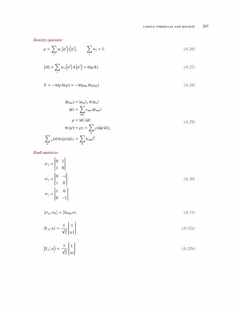
useful formulas and review 297
Density operator
ρ =∑
i
wi∣∣∣αi
⟩ ⟨αi
∣∣∣ , ∑i
wi = 1. (A.26)
[A] =∑
i
wi⟨αi
∣∣∣ A∣∣∣αi
⟩= tr(ρA). (A.27)
S = − tr(ρ ln ρ) = − tr(ρkk ln ρkk) (A.28)
|ψmn〉 = |am〉1 ⊗ |an〉
|ψ〉 =∑mn
cmn |ψmn〉
ρ = |ψ〉 〈ψ|
tr2(ρ) = ρ2 =∑
a2〈a|ρ |a〉2∑
a1〈a| tr2(ρ) |a〉1 =
∑n
|cmn|2
(A.29)
Pauli matrices
(A.30)
σx =
0 1
1 0
σy =
0 −i
i 0
σz =
1 0
0 −1
[σa, σb] = 2iεabcσc (A.31)
(A.32a)|S x;±〉 =1√
2
1
±1
(A.32b)
∣∣∣S y;±⟩
=1√
2
1
±i

298 useful formulas and review
(A.32c)|S z;±〉 =
10 ,
01
For n = (sin θ cos φ, sin θ sin φ, cos θ), the eigenkets of S · n are
|n; +〉 =
cos (θ/2) e−iφ/2
sin (θ/2) eiφ/2
= e−iσzφ/2e−iσyθ/2 |z; +〉 (A.33)
|n;−〉 =
− sin (θ/2) e−iφ/2
cos (θ/2) eiφ/2
= e−iσzφ/2e−iσy(θ+π)/2 |z; +〉 (A.34)
H = −e
mcS ·B = −
eBmc
S z (A.35)
Harmonic oscillator
(A.36)x20 =
hmω
(A.37)p20 = mω h
(A.38)x(t) =x0√
2
(ae−iωt + a†eiωt
)
(A.39)p(t) =i h√
2x0
(a†eiωt − ae−iωt
)a, a† =
1√
2x0
(x ∓ x2
0ddx
)(A.40)
(A.41)a |n〉 =√
n |n − 1〉
(A.42)a† |n〉 =√
n + 1 |n + 1〉
(A.43)x(t) = x(0) cosωt +p(0)mω
sinωt

useful formulas and review 299
(A.44)p(t) = p(0) cosωt − mωx(0) sinωt
(A.45)x(t)2 =hω2
(ae−iωt + a†eiωt
)2
(A.46)p(t)2 =hω2
(ae−iωt − a†eiωt
) (a†eiωt − ae−iωt
)
N = a†a (A.47)
N |n〉 = n |n〉 (A.48)
[N, a] = −a (A.49)
[N, a†
]= a† (A.50)
(A.51)H = hω(N +
12
)
(A.52)[a, a†
]= 1
(A.53)a =1
x0√
2
(x +
ipmω
)
〈x|n〉 =1
π1/4√
2nn!x−(n+1/2)
0
(x − x2
0ddx
)n
e−(x/x0)2/2 (A.54)
|n〉 =
(a†
)n
√n!|0〉 (A.55)

300 useful formulas and review
Coherent states
a |z〉 = z |z〉 (A.56)
|z〉 = e−|z|2/2+za† |0〉 (A.57)
〈z| aa† |z〉 = 〈z| 1 + a†a |z〉 (A.58)
(A.59)〈x〉 (0) = x0 ≡
√2 hmω
Re z =
√h
2mω(z + z∗)
〈p〉 (0) = p0 ≡√
2m hω Im z = −i
√m hω
2(z − z∗) .
Electromagnetism
(A′, φ′) = (A +∇χ, φ − ∂tχ) (A.60)
E = −∂A∂t−∇φ
B = ∇ ×A(A.61)
(A.62)A =
Bρ2
a2ρ φ if ρ ≥ ρa =⇒ B = 0
Bρ2 φ if ρ < ρa =⇒ B = Bz
Φ ≡∮
A · dl (A.63)
Aharonov-Bohm and Magnetic fields
H =1
2m
(p −
qc
A)
+ qφ (A.64)

useful formulas and review 301
Π = p −ec
A
[Πx,Πy] =ie hc
Bz
H =1
2mΠ2 = hω
(b†b +
12
)ω =
eB0
mc
b =1
√2mω h
(Πx + iΠy)
(A.65)
A =B0
2(−y, x, 0) ,A = B0 (0, x, 0) =⇒ B = B0z (A.66)
Dirac equation
H =
pc + V mc2
mc2 −pc + V
= pcσz + mc2σx + V (A.67)
ψ = e±ikx−iEt/ h
|+k;±ε〉 =
cos θ
sin θ
,− sin θ
cos θ
|−k;±ε〉 =
sin θ
cos θ
,− cos θ
sin θ
tan(2θ) = mc/ h|k|
ε2 =(mc2
)2+ ( hkc)2
(A.68)
ψ = e∓kx−iEt/ h
|±〉 =1√
2
±e±iφ/2
e∓iφ/2
ε2 =
(mc2
)2− ( hkc)2
eiφ =ε ± ik hc
mc2
(A.69)
j = cΨ†σzΨ (A.70)

302 useful formulas and review
Generators
Ta = e−ip·a/ h (A.71)
Tp = eip·x/ h (A.72)
(A.73)D(n, φ) = exp (−iJ · nφ/ h)
Calculus
∇2ψ =
1ρ∂ρ (ρ∂ρψ) +
1ρ2 ∂φφψ + ∂zzψ (A.74)
∇2ψ =
1r2 ∂r
(r2∂rψ
)+
1r2 sin θ
∂θ (sin θ∂θψ) +1
r2 sin2 θ∂φφ (A.75)
∫ ∞
−∞
exp(ax2)dx =
√−π
a(A.76)
Γ(t) =
∫ ∞
0xt−1e−xdx = (t − 1)! (A.77)
∫ ∞
0e−αrrndr =
n!αn+1 (A.78)
(A.79)limN →∞
(1 +
xN
)N= ex
Symmetries
(A.80)π† = π
= π−1
(A.81)π†xπ = −x
(A.82)π†pπ = −p

useful formulas and review 303
π |x〉 = |−x〉 (A.83)
〈x| π |ψ〉 = 〈−x|ψ〉 = ψ(−x) (A.84)
(A.85)[π, J] = 0
(A.86)ΘH = HΘ
(A.87)ΘpΘ−1 = −p
(A.88)ΘJΘ−1 = −J
(A.89)ΘxΘ−1 = x
(A.90)〈x|Θ |α〉 = 〈α|x〉
(A.91)Θ | j,m〉 = i2m | j,−m〉
(A.92)Θ2 = (−1)2 j
(A.93)
Θ = −iσyηK, η = i
Ki = −i
Θ |n; +〉 = η |n;−〉
Θ |n;−〉 = −η |n; +〉
Spin
(A.94)[Jx, Jy
]= i hJz
(A.95)[Jr, Js] = i hεrst Jt
(A.96)[J2, J±
]= 0
(A.97)[Jz, J±
]= ± hJ±
(A.98)[J+, J−] = 2 hJz
(A.99)J = L ⊗ 1 + 1 ⊗ S= L + S
(A.100)Jz | j,m〉 = m h | j,m〉
(A.101)J2 | j,m〉 = j( j + 1) h2 | j,m〉
(A.102)J± | j,m〉 = h√
( j ∓ m)( j ± m + 1) | j,m〉
(A.103)D(R) = exp (−iL · nφ/ h) ⊗ exp (−iS · nφ/ h)

304 useful formulas and review
Spin one representation
(A.104)Jx =h√
2
0 1 0
1 0 1
0 1 0
(A.105)Jy =hi√
2
0 −1 0
1 0 −1
0 1 0
(A.106)Jz = h
1 0 0
0 0 0
0 0 −1
.Angular momentum
(A.107)
L2 = L2z +
12
(L+L− + L−L+)
= − h2(
1sin2 θ
∂φφ +1
sin θ∂θ (sin θ∂θ)
)= x2p2 − (x · p)2 + i hx · p= r2p2 + h2
(r2∂rr + 2r∂r
)
Lx = −i h (− sin φ∂θ − cot θ cos φ∂φ)
Ly = −i h (cos φ∂θ − cot θ sin φ∂φ)
Lz = −i h∂φ
(A.108)
(A.109)[Lx, Ly
]= i hLz
L+, L− = 2(L2x + L2
y) = 2(L2 − L2z ) (A.110)
L± = −i he±iφ (±i∂θ − cot θ∂φ) = Lx ± iLy (A.111)

useful formulas and review 305
L± |l,m〉 = h√
(l ∓m)(l ±m + 1) |l,m ± 1〉 (A.112)
L2 |l,m〉 = l(l + 1) h2 |l,m〉 (A.113)
Lz |l,m〉 = m h |l,m〉 (A.114)
Spherical harmonics
Y00 =1
2√π
Y10 =12
√3π
cos(θ)
Y20 =14
√5π
(3 cos2(θ) − 1
)Y30 =
14
√7π
(5 cos3(θ) − 3 cos(θ)
)Y40 =
3((35 cos4(θ) − 30 cos2(θ) + 3
)16√π
Y50 =1
16
√11π
(63 cos5(θ) − 70 cos3(θ) + 15 cos(θ)
)Y60 =
132
√13π
(231 cos6(θ) − 315 cos4(θ) + 105 cos2(θ) − 5
)Y70 =
132
√15π
(429 cos7(θ) − 693 cos5(θ) + 315 cos3(θ) − 35 cos(θ)
)Y80 =
1256
√17π
(6435 cos8(θ) − 12012 cos6(θ) + 6930 cos4(θ) − 1260 cos2(θ) + 35
)
(A.115)
(A.116)Yl,−m = (−1)mY∗lm
FIXME: complete this table.

306 useful formulas and review
Hydrogen wavefunctions From [14], with the a0 factors added in.
ψ1s = ψ100 =1√π
(Za0
)3/2
e−Zr/a0 (A.117a)
ψ2s = ψ200 =1
4√
2π
(Za0
)3/2 (2 −
rZa0
)e−Zr/2a0 (A.117b)
ψ2px =1√
2(ψ2,1,−1 − ψ2,1,1) =
1
4√
2π
(Za0
)3/2 rZa0
e−rZ/2a0 sin θ cos φ (A.117c)
ψ2py =i√
2(ψ2,1,−1 + ψ2,1,1) =
1
4√
2π
(Za0
)3/2 rZa0
e−rZ/2a0 sin θ sin φ (A.117d)
ψ2pz = ψ210 =1
4√
2π
(Za0
)3/2 rZa0
e−rZ/2a0 cos θ. (A.117e)
I looked to [7] to see where to add in the a0 factors.Energy levels are n dependent only
(A.118)En = −Z2e2
2n2a0.
a0 =4πε0 h2
me2 (A.119)
Perturbation
H = H0 + λV (A.120a)
|n〉 =∑j=0
λ j∣∣∣n j
⟩(A.120b)
∆n =∑j=1
λ j∆n j (A.120c)

useful formulas and review 307
Pn =∑m,n
|m〉 〈m| (A.120d)
|n0〉 =∣∣∣n(0)
⟩|n1〉 =
Pn
E(0)n − H0
V |n0〉
|n2〉 =Pn
E(0)n − H0
(V − ∆n1) |n1〉
|n3〉 =Pn
E(0)n − H0
(V |n2〉 − ∆n1 |n2〉 − ∆n2 |n1〉)
∣∣∣n j⟩
=Pn
E(0)n − H0
V ∣∣∣n j−1⟩−
j−1∑k=1
∆nk
∣∣∣n j−k⟩
(A.121)
∆n j = 〈n0|V∣∣∣n j−1
⟩(A.122)
(A.123)f (|x|) = Θ(x) f (x) + Θ(−x) f (−x)
(A.124)ddxδ(x) = −
δ(x)x
Clebsch Ex. l1 = 2, l2 = 1
|3, 3〉 = |2, 2〉 ⊗ |1, 1〉
|3, 2〉 =1
〈3, 2| L− |3, 3〉((L− |2, 2〉) ⊗ |1, 1〉 + |2, 2〉 ⊗ L− |1, 1〉)
|2, 2〉 : a |1〉 + b |2〉 → −b |1〉 + a |2〉
|1, 1〉 = |3, 1〉 × |2, 1〉
(A.125)


BO D D S A N D E N D S
b.1 schwartz inequality in bra-ket notation
Motivation In [11] the Schwartz inequality
〈a|a〉 〈b|b〉 ≥ |〈a|b〉|2, (B.1)
is used in the derivation of the uncertainty relation. The proof of the Schwartz inequality usesa sneaky substitution that doesn’t seem obvious, and is even less obvious since there is a typoin the value to be substituted. Let’s understand where that sneakiness is coming from.
Without being sneaky My ancient first year linear algebra text [8] contains a non-sneaky proof,but it only works for real vector spaces. Recast in bra-ket notation, this method examines thebounds of the norms of sums and differences of unit state vectors (i.e. 〈a|a〉 = 〈b|b〉 = 1.)
(B.2)〈a − b|a − b〉 = 〈a|a〉 + 〈b|b〉 − 〈a|b〉 − 〈b|a〉 = 2 − 2 Re 〈a|b〉 ≥ 0,
so
(B.3)1 ≥ Re 〈a|b〉 .
Similarly
(B.4)〈a + b|a + b〉 = 〈a|a〉 + 〈b|b〉 + 〈a|b〉 + 〈b|a〉 = 2 + 2 Re 〈a|b〉 ≥ 0,
so
(B.5)Re 〈a|b〉 ≥ −1.
This means that for normalized state vectors
−1 ≤ Re 〈a|b〉 ≤ 1, (B.6)
or
(B.7)|Re 〈a|b〉| ≤ 1.
Writing out the unit vectors explicitly, that last inequality is
309

310 odds and ends
(B.8)
∣∣∣∣∣∣Re⟨
a√〈a|a〉
∣∣∣∣∣∣ b√〈b|b〉
⟩∣∣∣∣∣∣ ≤ 1,
squaring and rearranging gives
(B.9)|Re 〈a|b〉|2 ≤ 〈a|a〉 〈b|b〉 .
This is similar to, but not identical to the Schwartz inequality. Since |Re 〈a|b〉| ≤ |〈a|b〉| theSchwartz inequality cannot be demonstrated with this argument. This first year algebra methodworks nicely for demonstrating the inequality for real vector spaces, so a different argument isrequired for a complex vector space (i.e. quantum mechanics state space.)
Arguing with projected and rejected components Notice that the equality condition holdswhen the vectors are colinear, and the largest inequality (0 ≤ 1) holds when the vectors arenormal to each other. Given those geometrical observations, it seems reasonable to examine thenorms of projected or rejected components of a vector. To do so in bra-ket notation, the correctform of a projection operation must be determined. Care is required to get the ordering of thebra-kets right when expressing such a projection (or rejection)
Suppose we wish to calculation the rejection of |a〉 from |b〉, that is |b − αa〉, such that
(B.10)0 = 〈a|b − αa〉= 〈a|b〉 − α 〈a|a〉 ,
or
(B.11)α =〈a|b〉〈a|a〉
.
Therefore, the projection of |b〉 on |a〉 is
Proj|a〉 |b〉 =〈a|b〉〈a|a〉
|a〉 =〈b|a〉∗
〈a|a〉|a〉 . (B.12)
The conventional way to write this in QM is in the operator form
(B.13)Proj|a〉 |b〉 =|a〉 〈a|〈a|a〉
|b〉 .
In this form the rejection of |a〉 from |b〉 can be expressed as
(B.14)Rej|a〉 |b〉 = |b〉 −|a〉 〈a|〈a|a〉
|b〉 .
This state vector is normal to |a〉 as desired
B.2 an observation about the geometry of pauli x ,y matrices 311
(B.15)⟨a∣∣∣∣∣b − 〈a|b〉〈a|a〉
a⟩
= 〈a|b〉 −〈a|b〉
〈a|a〉〈a|a〉 = 0.
How about it’s length? That is
⟨b −〈a|b〉〈a|a〉
a∣∣∣∣∣b − 〈a|b〉〈a|a〉
a⟩
= 〈b|b〉 − 2|〈a|b〉|2
〈a|a〉+|〈a|b〉|2
〈a|a〉2〈a|a〉
= 〈b|b〉 −|〈a|b〉|2
〈a|a〉.
(B.16)
Observe that this must be greater to or equal to zero, so
〈b|b〉 ≥|〈a|b〉|2
〈a|a〉. (B.17)
Rearranging this gives eq. (B.1) as desired. The Schwartz proof in [11] obscures the geometryinvolved and starts with
(B.18)〈b + λa|b + λa〉 ≥ 0,
where the “proof” is nothing more than a statement that one can “pick” λ = − 〈b|a〉 /〈a|a〉.The Pythagorean context of the Schwartz inequality is not mentioned, and without thinkingabout it, one is left wondering what sort of magic hat that λ selection came from.
b.2 an observation about the geometry of pauli x ,y matrices
Motivation The conventional form for the Pauli matrices is
σx =
0 1
1 0
σy =
0 −i
i 0
σz =
1 0
0 −1
. (B.19)
In [2] these forms are derived based on the commutation relations
[σr, σs] = 2iεrstσt, (B.20)
by defining raising and lowering operators σ± = σx ± iσy and figuring out what form thematrix must take. I noticed an interesting geometrical relation hiding in that derivation if σ+ isnot assumed to be real.

312 odds and ends
Derivation For completeness, I’ll repeat the argument of [2], which builds on the commuta-tion relations of the raising and lowering operators. Those are
(B.21)
[σz, σ±
]= σz
(σx ± iσy
)−
(σx ± iσy
)σz
=[σz, σx
]± i
[σz, σy
]= 2iσy ± i(−2i)σx
= ±2(σx ± iσy
)= ±2σ±,
and
(B.22)
[σ+, σ−] =(σx + iσy
) (σx − iσy
)−
(σx − iσy
) (σx + iσy
)= −iσxσy + iσyσx − iσxσy + iσyσx
= 2i[σy, σx
]= 2i(−2i)σz
= 4σz
From these a matrix representation containing unknown values can be assumed. Let
(B.23)σ+ =
a b
c d
.The commutator with σz can be computed
(B.24)
[σz, σ+
]=
1 0
0 −1
a b
c d
−a b
c d
1 0
0 −1
=
a b
−c −d
−a −b
c −d
= 2
0 b
−c 0
Now compare this with eq. (B.21)
(B.25)
2
0 b
−c 0
= 2σ+
= 2
a b
d d
.

B.2 an observation about the geometry of pauli x ,y matrices 313
This shows that a = 0, and d = 0. Similarly the σz commutator with the lowering operator is
(B.26)
[σz, σ−
]=
1 0
0 −1
0 −c∗
b∗ 0
− 0 −c∗
b∗ 0
1 0
0 −1
=
0 −c∗
−b∗ 0
− 0 c∗
b∗ 0
= −2
0 c∗
b∗ 0
Again comparing to eq. (B.21), we have
(B.27)
−2
0 c∗
b∗ 0
= −2σ−
= −2
0 −c∗
b∗ 0
,so c = 0. Computing the commutator of the raising and lowering operators fixes b
(B.28)
[σ+, σ−] =
0 b
0 0
0 0
b∗ 0
− 0 0
b∗ 0
0 b
0 0
=
|b|2 0
0 0
− [0 00 −|b|2
]= |b|2
1 0
0 −1
= |b|2σz.
From eq. (B.22) it must be that |b|2 = 4, so the most general form of the raising operator is
(B.29)σ+ = 2
0 eiφ
0 0
.Observation The conventional choice is to set φ = 0, but I found it interesting to see the formof σx, σy without that choice. That is

314 odds and ends
(B.30)σx =
12
(σ+ + σ−)
=
0 eiφ
e−iφ 0
(B.31)
σy =12i
(σ+ − σ−)
=
0 −ieiφ
−ie−iφ 0
=
0 ei(φ−π/2)
e−i(φ−π/2) 0
.Notice that the Pauli matrices σx and σy actually both have the same form as σx, but the
phase of the complex argument of each differs by 90. That 90 separation isn’t obvious in thestandard form eq. (B.19).
It’s a small detail, but I thought it was kind of cool that the orthogonality of these matrix unitvector representations is built directly into the structure of their matrix representations.
b.3 operator matrix element
Weird dreams I woke up today having a dream still in my head from the night, but it was astrange one. I was expanding out the Dirac notation representation of an operator in matrix form,but the symbols in the kets were elaborate pictures of Disney princesses that I was drawing withforestry scenery in the background, including little bears. At the point that I woke up from thedream, I noticed that I’d gotten the proportion of the bears wrong in one of the pictures, andthey looked like they were ready to eat one of the princess characters.
Guts As a side effect of this weird dream I actually started thinking about matrix elementrepresentation of operators.
When forming the matrix element of an operator using Dirac notation the elements are ofthe form 〈row| A |column〉. I’ve gotten that mixed up a couple of times, so I thought it would behelpful to write this out explicitly for a 2 × 2 operator representation for clarity.
To start, consider a change of basis for a single matrix element from basis |q〉 , |r〉, to basis|a〉 , |b〉

B.4 generalized gaussian integrals 315
(B.32)
〈q| A |r〉 = 〈q|a〉 〈a| A |r〉 + 〈q|b〉 〈b| A |r〉
= 〈q|a〉 〈a| A |a〉 〈a|r〉 + 〈q|a〉 〈a| A |b〉 〈b|r〉
+ 〈q|b〉 〈b| A |a〉 〈a|r〉 + 〈q|b〉 〈b| A |b〉 〈b|r〉
= 〈q|a〉[〈a| A |a〉 〈a| A |b〉
] 〈a|r〉〈b|r〉
+ 〈q|b〉[〈b| A |a〉 〈b| A |b〉
] 〈a|r〉〈b|r〉
=
[〈q|a〉 〈q|b〉
] 〈a| A |a〉 〈a| A |b〉〈b| A |a〉 〈b| A |b〉
〈a|r〉〈b|r〉
.Suppose the matrix representation of |q〉 , |r〉 are respectively
(B.33)
|q〉 ∼
〈a|q〉〈b|q〉
|r〉 ∼
〈a|r〉〈b|r〉
,
then
(B.34)〈q| ∼
〈a|q〉〈b|q〉
†
=[〈q|a〉 〈q|b〉
].
The matrix element is then
(B.35)〈q| A |r〉 ∼ 〈q|
〈a| A |a〉 〈a| A |b〉〈b| A |a〉 〈b| A |b〉
|r〉 ,and the corresponding matrix representation of the operator is
(B.36)A ∼
〈a| A |a〉 〈a| A |b〉〈b| A |a〉 〈b| A |b〉
.b.4 generalized gaussian integrals
Both [11] and [16] use Gaussian integrals with both (negative) real, and imaginary arguments,which give the impression that the following is true:
(B.37)∫ ∞
−∞
exp(ax2
)dx =
√−π
a,

316 odds and ends
even when a is not a real negative constant, and in particular, with values a = ±i. Clearlythis doesn’t follow by just making a substitution x → x/
√a, since that moves the integration
range onto a rotated path in the complex plane when a is ±i. However, with some care, it can beshown that eq. (B.37) holds provided Re a ≤ 0.
To show this, this integral will be considered for the pure real case, purely imaginary, andfinally the complex case with non-zero real and imaginary parts for a.
Real (negative) case. The first special case is∫ ∞−∞
exp(−x2
)dx =
√π which is easy to derive
using the usual square it and integrate in circular coordinates trick.
Purely imaginary cases. Let’s handle the a = ±i cases next. These can be evaluated by con-sidering integrals over the contours of fig. B.1, where the upper plane contour is used for a = iand the lower plane contour for a = −i.
Figure B.1: Contours for a = ±i.
Since there are no poles, the integral over either such contour is zero. Credit for figuring outhow to tackle that integral and what contour to use goes to Dr MV, on stackexchange [6].
For the upper plane contour we have
(B.38)0 =
exp
(iz2
)dz
=
∫ R
0exp
(ix2
)dx +
∫ π/4
0exp
(iR2e2iθ
)Rieiθdθ +
∫ 0
Rexp
(i2t2
)eiπ/4dt.
Observe that ie2iθ = i cos(2θ) − sin(2θ) which has a negative real part for all values of θ , 0.Provided the contour is slightly deformed from the axis, that second integral has a term of theform ∼ Re−R2
which tends to zero as R→ ∞. So in the limit, this is

B.4 generalized gaussian integrals 317
(B.39)∫ ∞
0exp
(ix2
)dx =
√πeiπ/4/2,
or
(B.40)∫ ∞
−∞
exp(ix2
)dx =
√iπ,
a special case of eq. (B.37) as desired. For a = −i integrating around the lower plane contour,we have
(B.41)
0 =
exp
(−iz2
)dz
=
∫ R
0exp
(ix2
)dx +
∫ −π/4
0exp
(−iR2e2iθ
)Rieiθdθ +
∫ 0
Rexp
(−i(−i)t2
)e−iπ/4dt.
This time, in the second integral we also have −iR2e2iθ = iR2 cos(2θ) + sin(2θ), which alsohas a negative real part for θ ∈ (0, π/4]. Again the contour needs to be infinitesimally deformed1,placed just lower than the axis.
This time we find
(B.42)∫ ∞
−∞
exp(−ix2
)dx =
√−iπ,
another special case of eq. (B.37).
Completely complex case. A similar trick can be used to evaluate the more general cases,but a bit of thought is required to figure out the contours required. More precisely, while thesecontours will still have a wedge of pie shape, as sketched in fig. B.2, we have to figure out theangle subtended by the edge of this piece of pie.
To evaluate an integral consider
(B.43)0 =
∮exp
(eiφz2
)dz
=
∫ R
0exp
(eiφx2
)dx +
∫ θ
0exp
(eiφR2e2iµ
)Rieiµdµ +
∫ 0
Rexp
(eiφe2iθt2
)eiθdt,
where φ ∈ (π/2, π) ∪ (π, 3π/2). We have a hope of evaluating this last integral if φ + 2θ = π,or
(B.44)θ = (π − φ)/2,
1 Distorting the contour in this fashion seems somewhat like handwaving. A better approach would probably follow[5] where Jordan’s lemma is covered. It doesn’t look like Jordan’s lemma applies as is to this case, but the argumentslook like they could be adapted appropriately.
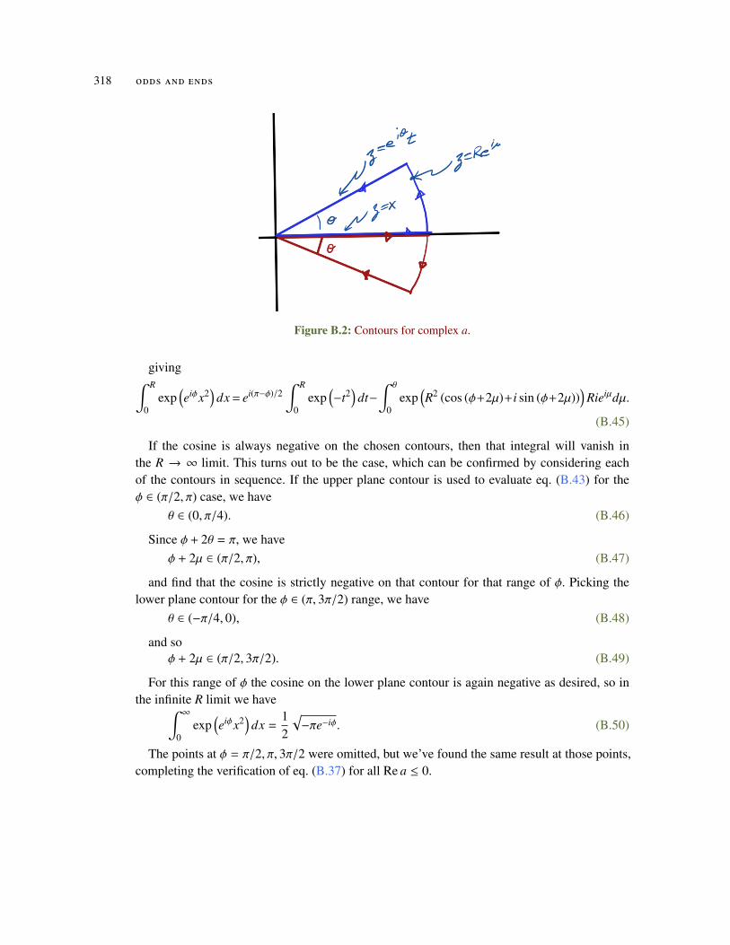
318 odds and ends
Figure B.2: Contours for complex a.
giving∫ R
0exp
(eiφx2
)dx = ei(π−φ)/2
∫ R
0exp
(−t2
)dt−
∫ θ
0exp
(R2 (cos (φ+2µ)+i sin (φ+2µ))
)Rieiµdµ.
(B.45)
If the cosine is always negative on the chosen contours, then that integral will vanish inthe R → ∞ limit. This turns out to be the case, which can be confirmed by considering eachof the contours in sequence. If the upper plane contour is used to evaluate eq. (B.43) for theφ ∈ (π/2, π) case, we have
(B.46)θ ∈ (0, π/4).
Since φ + 2θ = π, we have(B.47)φ + 2µ ∈ (π/2, π),
and find that the cosine is strictly negative on that contour for that range of φ. Picking thelower plane contour for the φ ∈ (π, 3π/2) range, we have
(B.48)θ ∈ (−π/4, 0),
and so(B.49)φ + 2µ ∈ (π/2, 3π/2).
For this range of φ the cosine on the lower plane contour is again negative as desired, so inthe infinite R limit we have
(B.50)∫ ∞
0exp
(eiφx2
)dx =
12
√−πe−iφ.
The points at φ = π/2, π, 3π/2 were omitted, but we’ve found the same result at those points,completing the verification of eq. (B.37) for all Re a ≤ 0.

B.5 a curious proof of the baker-campbell-hausdorff formula 319
b.5 a curious proof of the baker-campbell-hausdorff formula
Equation (39) of [3] states the Baker-Campbell-Hausdorff formula for two operators a, b thatcommute with their commutator [a, b]
(B.51)eaeb = ea+b+[a,b]/2,
and provides the outline of an interesting method of proof. That method is to consider thederivative of
(B.52)f (λ) = eλaeλbe−λ(a+b),
That derivative is
(B.53)
d fdλ
= eλaaeλbe−λ(a+b) + eλabeλbe−λ(a+b) − eλabeλb(a + b)e−λ(a+b)
= eλa(aeλb + beλb − eλb(a + b)
)e−λ(a+b)
= eλa([
a, eλb]
+
[b, eλb
])e−λ(a+b)
= eλa[a, eλb
]e−λ(a+b).
The commutator above is proportional to [a, b]
(B.54)
[a, eλb
]=
∞∑k=0
λk
k!
[a, bk
]=
∞∑k=0
λk
k!kbk−1 [a, b]
= λ
∞∑k=1
λk−1
(k − 1)!bk−1 [a, b]
= λeλb [a, b] ,
so
(B.55)d fdλ
= λ [a, b] f .
To get the above, we should also do the induction demonstration for[a, bk
]= kbk−1 [a, b].
This clearly holds for k = 0, 1. For any other k we have

320 odds and ends
(B.56)
[a, bk+1
]= abk+1 − bk+1a
=([
a, bk]
+ bka)
b − bk+1a
= kbk−1 [a, b] b + bk ([a, b] +ba
)−
bk+1a= kbk [a, b] + bk [a, b]= (k + 1)bk [a, b]
Observe that eq. (B.55) is solved by
(B.57)f = eλ2[a,b]/2,
which gives
(B.58)eλ2[a,b]/2 = eλaeλbe−λ(a+b).
Right multiplication by eλ(a+b) which commutes with eλ2[a,b]/2 and setting λ = 1 recovers
eq. (B.51) as desired.What I wonder looking at this, is what thought process led to trying this in the first place?
This is not what I would consider an obvious approach to demonstrating this identity.
b.6 position operator in momentum space representation
A derivation of the position space representation of the momentum operator −i h∂x is made in[2], starting with the position-momentum commutator. Here I’ll repeat that argument for themomentum space representation of the position operator.
What we want to do is expand the matrix element of the commutator. First using the definitionof the commutator
(B.59)⟨p′
∣∣∣ XP − PX∣∣∣p′′⟩ = i h
⟨p′
∣∣∣p′′⟩= i hδp′ − p′′,
and then by inserting an identity operation in a momentum space basis
(B.60)
⟨p′
∣∣∣ XP − PX∣∣∣p′′⟩ =
∫dp
⟨p′
∣∣∣ X |p〉 〈p| P∣∣∣p′′⟩ − ∫
dp⟨p′
∣∣∣ P |p〉 〈p| X∣∣∣p′′⟩
=
∫dp
⟨p′
∣∣∣ X |p〉 pδ(p − p′′) −∫
dppδ(p′ − p) 〈p| X∣∣∣p′′⟩
=⟨p′
∣∣∣ X∣∣∣p′′⟩ p′′ − p′
⟨p′
∣∣∣ X∣∣∣p′′⟩ .
So we have

B.7 expansion of the squared angular momentum operator 321
(B.61)⟨p′
∣∣∣ X∣∣∣p′′⟩ p′′ − p′
⟨p′
∣∣∣ X∣∣∣p′′⟩ = i hδp′ − p′′.
Because the RHS is zero whenever p′ , p′′, the matrix element 〈p′| X |p′′〉 must also includea delta function. Let
(B.62)⟨p′
∣∣∣ X∣∣∣p′′⟩ = δ(p′ − p′′)X(p′′).
Because eq. (B.61) is an operator equation that really only takes on meaning when applied toa wave function and integrated, we do that∫
dp′′δ(p′ − p′′)X(p′′)p′′ψ(p′′)−∫
dp′′p′δ(p′ − p′′)X(p′′)ψ(p′′) =
∫dp′′i hδp′ − p′′ψ(p′′),
(B.63)
or
(B.64)i hψ(p′) = X(p′)p′ψ(p′) − p′X(p′)ψ(p′).
Provided X(p′) operates on everything to its right, this equation is solved by setting
X(p′) = i h∂
∂p′. (B.65)
b.7 expansion of the squared angular momentum operator
In [11] eq. 6.16 is
L2 = x2p2 − (x · p)2+ i hx · p, (B.66)
and a derivation of the same. The derivation is clear right until the end, where the details forthe last steps are left off. When I attempted those last steps I got a different sign for the x · pterm. I also get that same difference in sign if I do this expansion myself:
(B.67)
L2 = εi jkxi p jεrskxr ps
= δ[rs]i j xi p jxr ps
= xi p jxi p j − xi p jx j pi
= xi(xi p j − i hδi j
)p j − xi p j
(pix j + i hδi j
)= x2p2 − i hx · p − xi p j pix j − i hx · p= x2p2 − 2i hx · p − xi pi p jx j
= x2p2 − 2i hx · p − (x · p)(x j p j − i h
)= x2p2 − i hx · p − (x · p)2.

322 odds and ends
I couldn’t spot an error anywhere above, but Prof Paramekanti spotted it when I asked. Theerror is in the second last step above, since p jx j = p1x1 + p2x2 + p3x3 and flipping the ordermust be done to each.
(B.68)L2 = x2p2 − 2i hx · p − (x · p)(x j p j − 3i h
)= x2p2 + i hx · p − (x · p)2.
The text is correct.

CJ U L I A N OT E B O O K S
These Julia notebooks, can be found inhttps://github.com/peeterjoot/julia.These notebooks are text files. The julia program, available freely at www.julialang.org, is
required to execute them. Some Julia code can also be evaluated with Matlab.
• Sep 24, 2015 phy1520/vectorSolenoid.jl
Plot of solenoid potential for constant interior magnetic field
• Nov 15, 2015 phy1520/rodbalancing.jl
Plug in some numbers for uncertainty time rod balancing calculation.
323


DM AT H E M AT I C A N OT E B O O K S
These Mathematica notebooks, some just trivial ones used to generate figures, others moreelaborate, and perhaps some even polished, can be found in
https://github.com/peeterjoot/mathematica/tree/master/.The free Wolfram CDF player, is capable of read-only viewing these notebooks to some
extent.
• Sep 28, 2015 phy1520/anticommutingWithZeroEigenvalue.nb
Construct and verify an example of a pair of anticommuting matrices each having a zeroeigenvalue, and a shared eigenvector. This was for Sakurai p.1.17, and includes somenumeric commutator expansions to verify the example constructions done with that prob-lem.
• Oct 25, 2015 phy1520/energyVsMomentumForDiracStepPotentialWaveFunctions.nb
A Manipulate to explore the energy vs momentum curves for a stepped potential barrierand the Dirac Hamiltonian.
• Nov 1, 2015 phy1520/spinOneHalfSymbolicManipulation.nb
For a spin one-half system Sakurai leaves it to the reader (and also to problem 3.10)to verify that knowledge of the three ensemble averages 〈S x〉 ,
⟨S y
⟩, 〈S z〉 is sufficient to
reconstruct the density operator. Showing that is algebraically messy, and well suited todo in Mathematica.
• Nov 2, 2015 phy1520/eulerAngleVsNormalRotationPauliMatrices.nb
Comparing a unimodular transformation to an arbitrary rotation matrix was trivial. Todo the same for an Euler angle rotation matrix and arbitrary matrix is less so becauseof sign differences. Here is a dumb symbol expansion of the full rotation on a generalvector in Pauli matrix form to have a look at the two results and see if there is anythingstriking. It turns out there is not anything striking. Both expressions are messy even afterFullSimplify.
• Nov 16, 2015 phy1520/spinOneOperatorRepresentation.nb
Spin one operators. Sakurai only seems to list the S y spin one matrix representation. Seethese in Desai, but need to verify that all my corrections to Desai eq. (27.117) are correct.
325

326 mathematica notebooks
• Nov 19, 2015 phy1520/diracDeltaFunctionIntegrals.nb
Double check the integral done in the Dirac delta function problem, and perform the firstFourier transformation.
• Nov 24, 2015 phy1520/spinOneDensityOperatorRepresentationInTermsOfEnsembleAverages.nb
Solution for Sakurai problem 3.12: What must we know in addition to the ensembleaverages of the spin operators to completely characterize the density matrix of a spin1 system? I guessed that we also needed the ensemble averages of at least the squares,but that and the unit trace, was not enough, since those relations do not provide nineequations, for the nine unknowns. Omitting the trace requirement, but also introducingvariables for the other second order products was enough to solve the problem. Printingout all those products is helpful to show why this is the case: you can see visually thatthese products appear to span the space of 3 × 3 matrices.
• Nov 24, 2015 phy1520/squareOfAngularMomentumOperatorSphericalCoordinates.nb
Expand out L in spherical coordinates in terms of Lx, Ly, Lz operators and compare tostated result (Sakurai (6.15)).
• Nov 26, 2015 phy1520/lecture19integralsAndPlots.nb
Confirm some of the lecture 19 (variational method) integrals, and plot the energy distri-bution.
• Dec 2, 2015 phy1520/visualizationOfEigenvaluesOfTwoByTwoHermitianMatrix.nb
Dynamic visualization of eigenvalues of 2 × 2 Hermitian matrix, as sketched in lecture20, plus some plots with specific values.
• Dec 3, 2015 phy1520/lecture21someSphericalHarmonicsAndTheirIntegrals.nb
Lecture 21. Print out some spherical harmonic functions and their integrals, to look at theconditions for the integral of Ylmz to be zero. Also evaluate the z and z2 brakets mentionedin the lecture.
• Dec 6, 2015 phy1520/sakuraiProblem5.13c.nb
Sakurai. Problem 5.11 (c). Verify hand calculations (diagonalization).
• Dec 8, 2015 phy1520/vanDerWalls.nb
Do a second order expansion of the van der Walls potential to compare to value stated.Did not figure out how to get Mathematica to simplify this gracefully and did it by handmanually instead.

mathematica notebooks 327
• Dec 10, 2015 phy1520/lecture22Integrals.nb
Integrals from lecture 22 (van der Walls potential).
• Dec 11, 2015 phy1520/sakuraiProblem3.17.nb
sakuraiProblem3.17
• Dec 13, 2015 phy1520/sakuraiProblem5.17a.nb
Sakurai pr. 5.17 (a): Find energy eigenvalues for H = AL2 + BLz + CLy.
• Dec 14, 2015 phy1520/commutatorOfRadialPortionOfMomentumSquaredOperator.nb
Compute the commutator[− h2
2mr2 ∂r(r2∂r),−i h∂r]
= − h2
2mr2 pr. The first operator is a com-ponent of p2/2m with the L2 contribution removed.
• Dec 14, 2015 phy1520/sakuraiProblem5.16bSHO.nb
Verify the relation from Sakurai pr. 5.16(a) using the ground state of the 3D SHO. Veri-fication of the potential derivative expectations for higher values of n do not complete inreasonable times.
• Dec 15, 2015 phy1520/sakuraiProblem3.33.nb
Spin three halves operator question (Sakurai 3.33). Implement operators for S +, S −, S z
that act on kets |±3/2〉 , |±1/2〉. These operators act on only a single basis element, but areused to construct the matrix representations for these operators (which are more general).Use those matrices to compute the representation of the Hamiltonian for the problem andcompute its energy eigenvalues. Display the end result and the representations for all ofS +, S −, S x, S y, S z,H = A(3S 2
z − S2) + B(S 2+ + S 2
−).
• Dec 15, 2015 phy1520/spinMatrices.nb
Compute and display S +, S −, S x, S y, S z, S 2 for a given spin (with h = 1). Use this todisplay the matrix representations of these operators for each of: spin 1/2, spin 1, spin3/2, spin 2, spin 5/2. Use this to solve the (spin one) eigensystem in Sakurai pr. 4.12.


Part III
I N D E X


I N D E X
Abelian group, 179Aharonov-Bohm effect, 75, 135, 137angular momentum, 189, 232
addition, 213, 214, 231azimthual quantum number, 205commutators, 224expectation, 234magnetic quantum number, 205Pauli matrix, 211perturbation, 288rotation operator, 210Schwinger, 206
angular momentum operator, 201anharmonic oscillator, 244, 272anti-unitary, 172anticommuting, 189applied electric field, 236approximation methods, 239associated Legendre polynomials, 213
basis, 4boost, 188braket, 4, 21
central force potential, 36classical Hamiltonian
Lorentz force, 91classical harmonic oscillator, 63Clebsch-Gordan, 219, 231coherent state, 65, 134
position operator, 69time evolution, 67uncertainty, 70
commutator
classical, 296polynomial functions, 51
correlation function, 112crystal spin, 198
degeneracy, 35, 47, 81, 263Stark effect, 263
density matrix, 55density operator, 10, 57
left observable, 15observable expectation, 14
dipole moment, 259Dirac equation, 145
boundary conditions, 155current, 161current density, 151diagonalization, 148free particle, 148plane wave, 147potential step, 163probability density, 151right going solution, 158scattering, 152, 163with potential, 148
Dirac sea, 149dispersion, 98distinguishable particles, 189double well potential, 246, 268
electric field, 73entanglement entropy, 16Euler angle, 230expectation, 4
coherent state, 68
331

332 Index
field theory, 71free particle, 128free particle propagator
momentum space, 127
gauge invariance, 72, 92gauge transformation, 93, 128
probability current, 132Gaussian integral, 315generator
translation, 179ground state, 126group, 173
Hamiltonian, 7non-Hermitian, 96symmetric real, 104two state, 29
harmonic oscillator, 63, 106anharmonic perturbation, 273ground state, 115perturbation, 266translation operator, 106variational method, 269xy perturbation, 275
Heisenberg picture, 10, 102coherent state, 67
helium-4, 269Hermite polynomial, 120hyperfine levels, 274
idempotent, 11infitesimal rotation, 179irreducible, 173
Jackiw-Rebbi problem, 162
Klein-Gordon equation, 146Kramer’s degeneracy, 187Kramer’s theorem, 188
ladder operator, 64Landau levels, 82
symmetric gauge, 136Little-Parks superconductor, 79Lorentz force, 131lowering operator, 64
magnetic field, 72, 73, 79, 226Mathematica, 58, 234, 238, 259, 265, 287,
290, 325matrix element, 314matrix representation, 24measurement, 8momentum
basis, 4expectation, 119operator, 6
momentum basis, 4
non-commuting observables, 35normalization, 4null operator, 26number operator, 64
orbital angular momentum, 201
pair creation, 149parity, 173, 189parity operator, 175particle in a box, 189partition function, 126Pauli matrix, 18, 59
orthonality, 311trace, 18
perturbation, 239, 248non-degenerate, 251simplest, 249
Poisson bracket, 50, 296probability
amplitude, 4
Index 333
current, 132density function, 4flux, 119
projection operator, 58propagator
free particle, 124
quadrupolar potential, 272
raising operator, 64reduced density
matrix, 56operator, 15
rotation, 19, 231determinant, 19
rotation invariance, 180
Schrödinger equationmomentum space, 109
Schrödinger picture, 9Schwartz inequality, 309similarity transformation, 49simultaneous eigenstate, 34, 47, 189spherical harmonics, 196, 212spherically symmetric potential
derivative, 284spin half, 56, 189, 225
dispersion, 30, 98ensemble averages, 56expectation, 62states, 28time reversal, 187two particles, 15
spin one, 188, 231spin precession, 93spin three halves, 236spin wave, 210Stark effect, 255state vector, 4Stern-Gerlach, 32
superconductor, 78symmetry
classical, 171group, 173unitary, 172
time evolution, 7, 9time reversal, 181, 188, 189, 196, 198
plane wave, 194properties, 183spinor, 194squared, 187
trace, 14translation
expectation, 54, 106generator, 188operator, 50, 177symmetry, 177
two stateperturbation, 280
uncertainty, 41unimodular transformation, 227unitary, 172unitary transformation, 48
van der Walls, 260multipole expansion, 265
variational method, 239, 244, 270vector operator, 201virial theorem, 104, 106
wave function, 4momentum space, 111
Zeeman effectquadratic, 290
zitterbewegung, 150, 162


Part IV
B I B L I O G R A P H Y


B I B L I O G R A P H Y
[1] Ronald M. Aarts. Commuting Matrices, 2015. URL http://mathworld.wolfram.com/CommutingMatrices.html. [Online; accessed 22-Oct-2015]. (Cited on page 39.)
[2] BR Desai. Quantum mechanics with basic field theory. Cambridge University Press, 2009.(Cited on pages 269, 311, 312, and 320.)
[3] Roy J Glauber. Some notes on multiple-boson processes. Physical Review, 84(3):395,1951. (Cited on page 319.)
[4] Eli Lansey. The Quantum Harmonic Oscillator Ladder Operators, 2009. URL http://eli.lansey.net/btg01-qhm.pdf. [Online; accessed 18-August-2015]. (Cited onpage 82.)
[5] W.R. Le Page and W.R. LePage. Complex Variables and the Laplace Transform for Engi-neers, chapter 8-10. A Theorem for Trigonometric Integrals. Courier Dover Publications,1980. (Cited on page 317.)
[6] Dr. MV. Evaluating definite integral of exp(i t^2), 2015. URL http://math.stackexchange.com/a/1411084/359. [Online; accessed 10-September-2015]. (Citedon page 316.)
[7] Carl R. Nave. Hydrogen Wavefunctions, 2015. URL http://hyperphysics.phy-astr.gsu.edu/hbase/quantum/hydwf.html. [Online; accessed 03-Dec-2015]. (Cited onpage 306.)
[8] W Keith Nicholson. Elementary linear algebra, with applications. PWS-Kent PublishingCompany, 1990. (Cited on page 309.)
[9] RK Pathria. Statistical mechanics. Butterworth Heinemann, Oxford, UK, 1996. (Cited onpage 127.)
[10] Jun John Sakurai and Jim J Napolitano. Errata: Typographical Errors, Mistakes, and Com-ments, Modern Quantum Mechanics, 2nd Edition, 2013. URL http://www.rpi.edu/dept/phys/Courses/PHYS6520/Spring2015/ErrataMQM.pdf. (Cited on page 88.)
[11] Jun John Sakurai and Jim J Napolitano. Modern quantum mechanics. Pearson Higher Ed,2014. (Cited on pages 16, 18, 19, 21, 24, 26, 28, 29, 30, 32, 34, 35, 41, 47, 48, 50, 51, 54,56, 87, 89, 93, 96, 98, 102, 104, 106, 109, 112, 115, 120, 121, 124, 126, 127, 128, 129,
337

338 bibliography
132, 134, 137, 189, 192, 194, 196, 198, 225, 226, 227, 230, 232, 234, 236, 266, 270, 275,280, 284, 288, 290, 309, 311, 315, and 321.)
[12] Jun John Sakurai and Jim J Napolitano. Modern quantum mechanics, chapter Time De-velopment of the Oscillator. Pearson Higher Ed, 2014. (Cited on page 82.)
[13] J Schwinger. Quantum theory of angular momentum. biedenharn l., van dam h., editors,1955. URL http://www.ifi.unicamp.br/~cabrera/teaching/paper_schwinger.pdf. (Cited on page 206.)
[14] Robert Field Troy Van Voorhis. Hydrogen Atom, 2013. URL http://ocw.mit.edu/courses/chemistry/5-61-physical-chemistry-fall-2013/lecture-notes/
MIT5_61F13_Lecture19-20.pdf. [Online; accessed 03-Dec-2015]. (Cited onpage 306.)
[15] Wikipedia. Baker-campbell-hausdorff formula — wikipedia, the free encyclope-dia, 2015. URL https://en.wikipedia.org/w/index.php?title=Baker%E2%80%93Campbell%E2%80%93Hausdorff_formula&oldid=665123858. [Online; accessed16-August-2015]. (Cited on page 106.)
[16] A. Zee. Quantum field theory in a nutshell. Universities Press, 2005. (Cited on page 315.)