peer influence and adolescent substance … · data for the study are from the ... health). the...
TRANSCRIPT

PEER INFLUENCE AND ADOLESCENT SUBSTANCE
USE: A SOCIAL NETWORKS ANALYSIS
By
MIYUKI VAMADEVAN ARIMOTO
A Dissertation submitted in partial fulfillment of the requirements for the degree of
Doctor of Philosophy
Washington State University Department of Sociology
MAY 2010
© Copyright by MIYUKI VAMADEVAN ARIMOTO, 2010
All Rights Reserved

© Copyright by MIYUKI VAMADEVAN ARIMOTO, 2010 All Rights Reserved
ii
To the Faculty of Washington State University:
The members of the Committee appointed to examine the dissertation of MIYUKI
VAMADEVAN ARIMOTO find it satisfactory and recommend that it be accepted.
___________________________________ Steven R. Burkett, Ph.D., Chair
____________________________________
Jennifer Schwartz, Ph.D.
____________________________________ Monica Kirkpatrick Johnson, Ph.D.

iii
ACKNOWLEDGMENTS
This research uses data from Add Health, a program project directed by Kathleen
Mullan Harris and designed by J. Richard Udry, Peter S. Bearman, and Kathleen Mullan Harris
at the University of North Carolina at Chapel Hill, and funded by grant P01-HD31921 from the
Eunice Kennedy Shriver National Institute of Child Health and Human Development, with
cooperative funding from 23 other federal agencies and foundations. Special acknowledgment
is due Ronald R. Rindfuss and Barbara Entwisle for assistance in the original design.
Information on how to obtain the Add Health data files is available on the Add Health website
(http://www.cpc.unc.edu/addhealth). No direct support was received from grant P01-HD31921
for this analysis.
My chair, Steven R. Burkett, has devoted his countless time and inexhaustible effort to
help me going through the entire process. His patience, professional advice and knowledge,
and academic as well as emotional support led me to reach this point. I could not ask for Steve
more than what he has offered. I am very proud to have been under his supervision during the
course of my graduate life at WSU.
My other two committee members, Jennifer Schwartz and Monica Kirkpatrick Johnson
have always shown their concerns about my progress and encouraged me to complete my
dissertation. Monica provided me with her statistical skills to deal with the complicated data.
Jennifer’s emotional support guided me to cross the finishing line.
My dearest friends, Fiona and Clint Cole, deserve many thanks. They are my best
friends ever and are an important part of my life. Without Fiona and Clint, I could not have
reached this stage. Last but not least, I would like to thank to my family who always spurred,
emotionally supported, and loved me as I sought to complete the degree.

iv
PEER INFLUENCE AND ADOLESCENT SUBSTANCE
USE: A SOCIAL NETWORK ANALYSIS
Abstract
By Miyuki Vamadevan Arimoto, Ph.D. Washington State University
May 2010
Chair: Steven R. Burkett
The relationship between delinquency involvement and association with delinquent
peers is well known among theorists and researchers. Although friendship relations are an
important aspect of adolescent life, only rarely is the structure of these relations examined
systematically. This study uses social network analysis as a tool to examine how association
with peers affects adolescent substance use.
Data for the study are from the National Longitudinal Study of Adolescent Health (Add
Health). The network characteristics examined include Centrality, Prestige, Density, and
Heterogeneity. Two types of analyses are presented: a quantitative analysis and a case study.
The quantitative study includes a regression analysis of the effects of the social network
variables on imminent and later substance use, and an analysis of use trajectory. The case
study provides a visual representation of the link between friendship groups and substance use.
The results from the quantitative study suggest that of the four network variables
examined only Prestige and Density have significant short-term effects on substance use.
Prestige has a positive effect and Density has a negative effect. The results regarding
Centrality and Heterogeneity are inconclusive although Centrality does appear to have a
v
negative effect on substance use when the race/ethnicity of the respondents is controlled.
Heterogeneity has a significant positive effect only for future illegal substance use. The
trajectory analyses reveal that trajectories for alcohol use and marijuana use trend in opposite
directions. The trajectory for alcohol use shows an increasing number of users and levels of
individual use, while that for marijuana use shows a decrease in both numbers of users and
levels of use. The case study examines the entire network of a small school. The results are
generally consistent with and illustrative of the results from the quantitative study. In addition,
the results suggest that individuals who are in structurally similar positions in a friendship
group engage in similar levels of substance use.
The research highlights the importance of peer network structures for understanding the
relationship between peer association and substance use. Limitations of the study are discussed
as are policy implications. Recommendations for future research are also suggested.

vi
TABLE OF CONTENTS
page ACKNOWLEDGMENTS .................................................................................................. iii
ABSTRACT ....................................................................................................................... iv
LIST OF TABLES ............................................................................................................. ix
LIST OF FIGURES ............................................................................................................ xi
DEDICATION .................................................................................................................. xii
CHAPTER
1. INTRODUCTION ............................................................................................. 1
2. THE THEORETICAL CONNECTIONS BETWEEN PEERS AND SUBSTANCE USE ........................................................................................... 5
Introduction ................................................................................................. 5
Friendships and delinquency ....................................................................... 5
Theoretical explanations of peer influence and co-offending ..................... 7
Patterns of youthful offending ................................................................... 16
Career Offending ....................................................................................... 21
Empirical Studies using Social Network Analysis .................................... 26
3. HYPOTHESES ................................................................................................ 33
4. METHODS ...................................................................................................... 42
Introduction ............................................................................................... 42
Study Design and Sample .......................................................................... 42
Dependent Variables ................................................................................. 45
Independent Variables ............................................................................... 47
Control Variables ....................................................................................... 51

vii
Analytical Strategy .................................................................................... 52
5. QUANTITATIVE STUDY: FINDINGS AND DISCUSSION ...................... 56
Introduction ............................................................................................... 56
Hypothesis 1 .............................................................................................. 56
Alcohol Use ................................................................................... 58
Marijuana Use ............................................................................... 68
Hypothesis 2 .............................................................................................. 77
Alcohol Use ................................................................................... 77
Marijuana Use ............................................................................... 80
Drinking Related Problems ........................................................... 82
Drug Use ........................................................................................ 86
Hypothesis 3 .............................................................................................. 90
Summary .................................................................................................. 102
6. CASE STUDY: FINDINGS AND DISCUSSION ........................................ 104
Introduction ............................................................................................. 104
Findings ................................................................................................... 106
Description of Sociograms for Alcohol Use and Marijuana Use ............ 106
The Effects of Network Variables on Alcohol and Marijuana Use ......... 108
Structural Equivalence ............................................................................. 113
Summary and Conclusion ........................................................................ 118
7. SUMMARY AND CONCLUSION .............................................................. 120
Discussion .................................................................................... 120
Limitations ................................................................................... 126
viii
Policy Implications ...................................................................... 128
Conclusion ................................................................................... 132
BIBLIOGRAPHY ........................................................................................................... 134
APPENDIX
A. Variable Descriptions ..................................................................................... 144
B. Measurement of Alcohol Related Problems ................................................... 145
C. Illicit Drug Use ............................................................................................... 146

ix
LIST OF TABLES
1. Multicollinearity Diagnostic .......................................................................................... 50
2. Logistic Regression Diagnostics for Specification Error .............................................. 51
3. Descriptive Statistics for the Quantitative Study (N=8,085) ......................................... 52
4. Descriptive Statistics for the Case Study (N=61) .......................................................... 53
5. Correlation Matrix for All Variables ............................................................................. 59
6. Network Characteristics on Alcohol Use at Wave II (N=7,106) ................................... 60
7. The Effects of the Network Variables on Alcohol Use When Attachment to Parents is Held Constant (N=7,040) .............................................................................. 62 8. ANOVA for Difference in Alcohol Use at Wave II (N=8,036) .................................... 64
9. Interaction Effects with Network Characteristics on Alcohol Use at Wave II (N=7,040) ................................................................................................... 65 10. Network Effects on Alcohol Use at Wave II by Race/Ethnicity ................................. 66
11. Network Characteristics on Marijuana Use at Wave II (N=6,943) ............................. 69
12. The Effects of the Network Variables on Marijuana Use When Attachment to Parents is Held Constant (N=6,943) ............................................................................ 72 13. ANOVA for Difference in Marijuana Use at Wave II (N=7,942) .............................. 73
14. Interaction Effects with Network Characteristics on Marijuana Use at Wave II (N=6,943) .................................................................................................. 74 15. Network Effects on Marijuana Use at Wave II by Race/Ethnicity ............................. 76
16. Correlation Matrix among Dependent Variables at Waves II and III ......................... 78
17. Network Effects on Alcohol Use at Wave III (N=6,845) ............................................ 79
18. Network Effects on Marijuana Use at Wave III (N=6,526) ........................................ 81
19. The Effect of Early Alcohol Use on Binge Drinking at Wave III ............................... 82
20. The Effect of Early Alcohol Use on Binge Drinking at Wave III by Race/Ethnicity ........................................................................................................ 83

x
21. Network Effects on Binge Drinking at Wave III (N=6,436) ....................................... 83
22. The Effect of Early Alcohol Use on Alcohol-Related Problems at Wave III (N=7,404) ................................................................................................. 85
23. The Effect of Early Alcohol Use on Alcohol-Related Problems at Wave III by Race/Ethnicity ........................................................................................................ 85
24. The Effect of Early Alcohol Use on Alcohol-Related Problems at Wave III Attenuated by Network Variables (N=6,436) ............................................................. 86
25. The Effect of Early Marijuana Use on Other Drug Use at Wave III (N=7,659) ......... 87
26. The Effect of Early Marijuana Use on Other Drug Use at Wave III by Race/Ethnicity ........................................................................................................ 87
27. Network Effects on Other Drug Use at Wave III (N=6,436) ...................................... 88
28. The Effect of Alcohol Use at Wave II on Alcohol Use at Wave III by Race/Ethnicity ........................................................................................................ 91
29. The Effect of Marijuana Use at Wave II on Marijuana Use at Wave III by Race/Ethnicity ........................................................................................................ 91
30. Fit Indices from One-trajectory to Five-trajectory Mixture Models for Alcohol Use ........................................................................................................... 94
31. Fit Indices from One-trajectory to Five-trajectory Mixture Models for Marijuana Use ........................................................................................................ 99
32. Hypothetical Non-Directional Network Matrix ........................................................ 104 33. Hypothetical Directional Network Matrix ................................................................. 105 34. Network Characteristics Held by Actors ................................................................... 111 35. Levels of Attachment to Parents ................................................................................ 113 36. Structural Equivalence Matrix (Pearson Correlation) ............................................... 115
xi
LIST OF FIGURES
1. Selection vs. Socialization Model ................................................................................. 13
2. The Growth Trajectory for Alcohol Use for the One-trajectory Latent Variable Growth Mixture Model ........................................................................ 92
3. Observed Levels of Alcohol Use ................................................................................... 93
4. The Three-trajectory Latent Variable Growth Mixture Model for Alcohol Use ........... 95
5. Trajectories of Alcohol Use among White Youth ......................................................... 96
6. Trajectories of Alcohol Use among African American Youth ...................................... 96
7. Trajectories of Alcohol Use among Asian Youth ......................................................... 97
8. Trajectories of Alcohol Use among Hispanic Youth .................................................... 98
9. Trajectories of Alcohol Use among Native American Youth ....................................... 99
10. The Three-trajectory Latent Variable Growth Mixture Model for Marijuana Use ... 100
11. Trajectories of Marijuana Use among White Youth ................................................. 100
12. Trajectories of Marijuana Use among African American Youth .............................. 101
13. Trajectories of Marijuana Use among Asian Youth .................................................. 101
14. Trajectories of Marijuana Use among Hispanic Youth ............................................. 102
15. Trajectories of Marijuana Use among Native American Youth ................................ 102
16. A Non-Directional Sociogram ................................................................................... 105
17. A Directional Sociogram ........................................................................................... 106
18. School-based Friendships and Alcohol Use .............................................................. 109
19. School-based Friendships and Marijuana Use .......................................................... 110
20. Example of Structural Equivalence ........................................................................... 114
21. Structural Equivalence among Substance Users ....................................................... 116

xii
Dedication
This dissertation is dedicated to my mother, father, brother, and maternal relatives who
provided both emotional and financial support.
1
CHAPTER ONE
INTRODUCTION
For decades, the relationship between peers and delinquency involvement has occupied
the attention of theorists and researchers (see Shaw and McKay 1931; Sutherland 1947; Glueck
and Glueck 1950; Cohen 1955; Shaw 1966; Hirschi 1969; Jensen 1972; Akers et al. 1979;
Krohn et al. 1982; Haynie 2001, 2002; Warr and Stafford 1991; Akers and Lee 1996, 1999; Lee
et al. 2004). A wide range of criminological or delinquency theories have been offered to
explain various forms of substance use either in general or specific (Akers 1992). It is clear
that most youthful offending, including substance use, is group or companion-based (Erickson
1971, 1973; Erickson and Jensen 1977; Reiss 1988; Warr 2002). Not only is there a strong
correlation between delinquency involvement and association with delinquent peers, but
typically juveniles commit delinquent acts in the company of others (Warr 2002).
In the case of substance use, youthful offenders rely on a social network to access
alcohol and/or drugs (Wagenaar et al. 1993; U.S. Department of Health and Human Services
2004; Finn 2006). Therefore, understanding how peer groups are formed and maintained is
vital to understanding much youthful substance use. However, although friendship relations
are an important aspect of an adolescent’s life, only rarely are the structures of these relations
examined systematically. In this study, I examine the structures of these associations as they
relate to youthful substance use.
Although both substance use and delinquency in general contravene legal and societal
standards for adolescents, these behaviors appear to exhibit distinct differences. According to
Maggs and Hurrelmann (1998: 370-371), there are five distinctions between substance use and

2
delinquency: 1) substance use is statistically normative while delinquent behavior is relatively
infrequent for adolescents; 2) substance use is considered a developmental task that may be
considered by some to be “healthy exploration” whereas delinquent behavior is not; 3) some
substance use such as drinking is a status offense while most delinquent behaviors including the
use of other substances such as marijuana are criminal offenses; 4) some substance use such as
drinking can be viewed as prosocial behavior whereas most delinquent behavior is considered
to be antisocial behavior; and, 5) substance use is categorized as a victimless crime while most
delinquent behavior is against other people, property, or environment.
The most recent Monitoring the Future survey in 2006 showed an overall decline in
substance use. However, certain drugs such as prescription drugs and tranquilizers continue to
have relatively high rates of use (see Johnston et al. 2007). Further, as McCurley and Snyder
(2008) note, 35 percent of youth between ages 15 and 17 report using alcohol and 14 percent
report marijuana use. These rates suggest that adolescents no doubt consider low levels of
alcohol and marijuana use to be relatively acceptable behavior.
Association with one’s peers is no doubt an important aspect of an adolescent’s life.
However, traditional measures of peer influence such as the number of delinquent friends youth
may have are often criticized because such measures say little about the quality of these
relationships or one’s location in a group (see, Zhang and Messner 2000). An alternative
measurement of peer influence is based on proximity to others in friendship structures using a
social network approach as a tool (see Snijders and Baerveldt 2003). The structures of
friendship relations are translated into several network variables that describe how adolescents
are enmeshed in different groups. The network variables are then quantified based on one’s

3
relational ties to others. By doing so, the relationship between peer association and substance
use can be examined systematically.
In addition, network variables are measured not only in terms of an individual’s
perceptions of where they may fit in a group, but also how others think the individual is
embedded in a particular network. Adolescents do not co-offend with mere acquaintances, but
with others who recognize and acknowledge them as members of a group. Therefore, network
variables tap into the nature of one’s interpersonal relationships and should aid in our
understanding of the dynamics of co-offending including the use of illegal substances.
This research addresses a central concern and several related questions. The primary
question is: How do social network characteristics affect substance use? That is, does the way
friendships form provide greater opportunities for some to learn about and engage in substance
use; and, do individuals who share similar or structurally equivalent positions in a group
demonstrate similar levels of substance use? A related issue is whether and how early
friendship network structures influence later substance use and, if they do, do those early peer
networks function as a facilitating or constraining factor over time? That is, is one’s structural
position in adolescent friendship groups related to substance use in one’s early to mid-twenties;
and, is the correlation between early alcohol and marijuana use and subsequent more serious
substance use attenuated by these early network characteristics? Finally, are the trajectories for
different types of substance use over time the same or different?
To answer these research questions, this study includes two separate analyses: a
quantitative analysis and a case study. In the quantitative analysis, I examine the relationships
between a set of peer network characteristics and adolescent substance use. I subsequently
focus on identifiable friendship groups within one school to illustrate the results of the
4
quantitative study. In the case study, I examine how individuals are connected and determine
the levels of substance use among and within peer groups. I also examine whether individuals
who have structurally similar positions in their peer group exhibit similar levels of substance
use.
Chapter 2 includes a review of past research that examines how friendships influence
delinquency involvement in general and substance use in particular. Theories that can be used
within a network approach to explain substance use are examined as well. This review includes
previous research on co-offending and gang studies, both of which focus on peer group
structures. The hypotheses to be examined in this study are presented in Chapter 3. A
description of data, the measurement of social network and other variables, and the analytical
procedures to be used are discussed in Chapter 4. The analysis and findings are presented in
Chapters 5 and 6. In the final chapter, limitations of this study are discussed as are the policy
implications of the findings.

5
CHAPTER TWO
THE THEORETICAL CONNECTIONS BETWEEN PEERS AND SUBSTANCE USE
Introduction
In general, research suggests that peer associations strongly influence delinquency
involvement, though the nature of that influence remains a matter of debate. For some,
delinquent behavior is a result of socialization to peer group norms that support delinquency
involvement (Akers 1998). For example, Warr (1993b) reports that exposure to delinquent
friends at an early age predicts subsequent delinquency involvement (see also, Akers et al.
1979; Krohn et al. 1984; Akers 1992; Akers and Lee 1999). Thus, the influence of delinquent
peers is considered to be a primary factor that leads juveniles to learn values that support
delinquent behavior (Akers 1998). On the other hand, some note that delinquent youth do not
associate exclusively with delinquent peers. For example, Matza (1964) argues that juveniles
“drift” between the conventional and unconventional relationships. In other words, some youth
maintain conventional relationships with their parents and non-delinquent peers, while entering
into often transitory relationships with delinquent peers. Thus, for some, friendship networks
overlap providing a bridge connecting relationships with both delinquent and non-delinquent
youth.
Friendships and Delinquency
Although friendship relations are an important, though variable, aspect of adolescent
life, only rarely are the structures of these relations examined systematically. Compared to
kinship relations (Willmott 1986), friendships are based upon personal choice and mutual
agreement to be in a relationship. Further, friendship relations are dynamic over time, that is,
6
some are maintained while others change or dissolve depending on circumstances (Zeggelink
1993: 7-8). It would seem that people can more easily walk away from friendships by
following their emotions or due to disinterest. Nevertheless, it seems likely that friendships
play some role both in facilitating and constraining delinquent behavior.
McAdams (1988) characterizes friendship as providing an individual with a sense of
belonging and as a source of emotional or physical support and reassurance of self-worth.
Although friendships may be prompted by different motives including profit or coercion
(Zeggelink 1993: 9), they nevertheless reflect a person’s lifestyle, gender, and cognitive state of
development (Hays 1988). Depending upon the context, all these factors can be a “drive” to
enter into a friendship group. Friendships are also affected by context. For example, for many
adolescents, friendships are school-based (see Coleman 1961; Polk and Schafer 1972). Youth
tend to form friendships with peers who attend the same school where they spend much of their
time interacting with one another in classes and school related activities. These friendships are
no doubt influenced at least in part by the various forms of evaluation that occur in the school
context, such as grades, as well as common interests that attract youth to specialized school-
sponsored interest groups and activities. In addition, since school districts typically determine
what school an adolescent will attend, friendship networks are likely to be relatively
homogeneous in terms of demographics such as race and social class.
A handful of studies focus specifically on “friendships” and delinquency (see Krohn
1986; Sarnecki 1986; Warr and Stafford 1991; Krohn and Thornberry 1993; Baerveldt and
Snijders 1994; Thornberry et al. 1994; Haynie 2002, 2001; Haynie and Osgood 2005). For
example, Warr (1993b) reports that peer culture provides an environment that is tolerant of
delinquency. Thornberry et al. (1994) examine the relationship between peer association and

7
delinquency involvement. Consistent with Warr’s findings (1993b), they report that social
environments in which peer culture encourages delinquency leads to delinquent behavior.
Although these studies suggest that juveniles learn from or are influenced by friendship groups,
how and what they learn is not always entirely clear.
In one recent study, Haynie (2002) examines the impact of the role of friendship
networks on delinquency and reports findings consistent with the central proposition of
Sutherland’s (1947) theory of differential association. That is, juveniles learn antisocial
behavior through direct contact with others in their age group. Baerveldt and Sniders (1994)
also find that pupils whose networks include friends who commit offenses are more likely to
commit offenses themselves. Similarly, Warr and Stafford (1991) report that the behavior of
delinquent friends has a greater effect on juveniles’ delinquency than friends’ attitudes toward
delinquency. Sarnecki (1986) also finds that juveniles who belong to delinquent groups are
more actively engaged in delinquency when they associate with other delinquents as members
of a group. They show an even greater risk of persistent offending than those who used to, but
no longer belong to a delinquent group. In sum, the concept “friendship” refers to something
more than a simple association with peers. It refers to structural connections among group
members that may be important to our understanding of the statistical association between peer
involvement and delinquency, including substance use.
Theoretical Explanations of Peer Influence and Co-offending
Like many criminological theories, Akers’ social learning theory (1998) focuses
specifically on the role of peers. He notes that typically the primary learning source for youth
is their parents or family, but that friends become more influential as youth grow older and gain
independence and autonomy from parents. According to Akers (1998), adolescents learn
8
antisocial behavior through the association with delinquent peers who reinforce definitions
favorable to involvement in such behavior. As they are socialized within peer groups, they
develop and adhere to group norms that support delinquent behavior.
Following the lead of Sutherland (1947), Akers’ key concept is “definitions favorable to
the violation of the law,” which refers to one’s attitudes toward certain behaviors as legal or
illegal, right or wrong (Akers 2000: 76). Extending Sutherland’s theory of differential
association, Akers argues that these “definitions” are acquired through three processes:
differential association, differential reinforcement, and imitation. Unlike Sutherland, Akers’
position is that youth learn behavior through both direct and indirect interaction with peers.
Differential association refers to “the process whereby one is exposed to normative
definitions favorable or unfavorable to” a certain behavior (Akers 2000: 76). Akers argues that
differential association refers to direct and indirect “association and interaction with others”
(76). Sutherland (1947: 6-7) stated in his seventh proposition in the theory of differential
association that the effect of such associations are greater when they are formed early in life
(“priority”), when the period of time such associations are maintained is extended (“duration”),
and more frequent (“frequency”), and when the other involved are important to them
(“intensity”). Consistent with Sutherland’s position, but with revisions based on behavioral
concepts and propositions, Akers extends the theory of differential association by introducing
the concept of “differential reinforcement” (Akers 1998: 45).
Differential reinforcement refers to the balance between the anticipated rewards and
costs derived from a behavior. That is, people behave in certain ways depending on the ratio of
rewards/costs. When the costs, such as punishment, are greater than the anticipated rewards,
juveniles are less likely to engage in delinquent behavior (Akers 1998: 68). Reinforcement that

9
increases the probability of committing delinquent behavior may be given positively or
negatively. This includes positive reinforcement such as praise that encourages delinquent
behavior. It may also include negative reinforcement such as negative comments in the form of
name calling directed toward youth who initially resist participating in delinquent acts.
Reinforcement is provided through the amount of profit that juveniles gain, the frequency of
reinforcement, and the probability of alternative options (68).
Similarly, punishment may be given both positively and negatively. Positive
punishment refers to the presentation of an unpleasant event such as being arrested, whereas
negative punishment refers to reduction or loss of privileges such as restrictions on TV time or
a reduction of monthly allowance. Punishment may come from within or from others, and may
include feeling sick after using drugs or drinking (see also Akers 1998: 66-75). Punishment,
especially that given by others, may make juveniles restrain from delinquent behaviors.
However, even when punishment is given, if the amount is too little compared to positive
reinforcement, juveniles are likely to engage in delinquent behavior and to do so continuously.
Finally, imitation refers to engaging in certain behaviors after observing similar
behaviors by others (Akers 2000: 79). Although most past research has focused on differential
association and differential reinforcement, a few scholars note that peer pressure to conform to
group norms is often acquired largely through imitation with or without much in the way of
reinforcement from others (see, for example, Warr and Stafford 1991). The question is, under
what conditions do youth observe and imitate the antisocial behavior of their peers? The
answer may be that structural proximity to delinquent friends increases the opportunity to be
exposed to delinquent behavior and that close observation results in delinquency involvement.
In other words, structurally core members may have more opportunities to witness certain

10
behaviors than with fringe members. For example, in his study of delinquent gangs, Fleisher
(2002) reports that core members were more likely to engage in antisocial behaviors due to
their proximity within the group.
Past research provides strong empirical support for social learning theory when
explaining substance use (Akers 2000: 89). For example, in the first of a series of empirical
studies, Akers et al. (1979) closely examined the effect of social learning variables. They
report that combined, the four key social learning variables, that is, differential association,
definition, differential reinforcement, and imitation, explain 55 percent of the variance in
alcohol use and 68 percent in marijuana use by adolescents. Further, Akers argues that we
learn both conventional and unconventional behavior, and that initiation and desistance of
substance use are the products of learning.
Although it is inarguable that there is a strong correlation between involvement with
delinquent peers and substance use (see Warr and Stafford 1991), it is questionable whether
youth are “transformed” by mere association with delinquent peers. For example, peer
influence is an important predictor of substance use, but when it comes to co-offending, that is,
the joint participation in illegal activities (Reiss 1988), juveniles do not commit these acts with
mere acquaintances (Warr 1996; Weerman 2003). However, “being friends” is not a necessary
condition to co-offend. Rather, a common incentive or reward gained from an offense must
exist between co-offenders (Weerman 2003). It seems likely that at least part of the correlation
between delinquency and association with delinquent peers is a function of social selection.
That is, juveniles who have already developed dispositions favorable to delinquent behavior are
more likely to choose delinquents as friends and may eventually commit delinquent acts
together. Morash (1983) reports that boys who belong to delinquent peer groups have above-
11
average rates of previous involvement in delinquent activities. When it comes to substance use,
Warr (2002: 81) notes that “drug use could be the raison d’être that brings a group together.”
Substance use requires co-dependence on others; thus, what may be referred to as “co-
offending” is very common.
“Co-offending,” according to Reiss (1988), refers to joint participation in illegal
behaviors. Therefore, co-offending is different from simple association with delinquent peers
and it is also more common among juveniles than among adults (Warr 1996; Weerman 2003).
Without a strong sense of belonging or connection to delinquent others, juveniles are unlikely
to commit offenses together. Although Hirschi approached delinquency differently by asking
why juveniles do not engage in delinquent behavior, this perspective can be applied to help
explain co-offending. Hirschi’s (1969) notion of social bonds and social selection is, perhaps,
particularly relevant. He explains that social ties to conventional others and/or institutions
restrain delinquent behavior, but when these ties are weakened juveniles are more likely to
“choose the wrong crowd” and engage in delinquent behavior. However, he questions whether
juveniles maintain strong attachments to these unconventional peers (1969: 159).
Hirschi (1969) identifies four elements which he refers to as the “social bond,” that is,
attachment, commitment, involvement, and belief. He argues that when juveniles have strong
attachments to conventional others such as parents or family, the school, and peers, when they
have a strong commitment to conventional goals, and when they are engaged in or spend time
in conventional activities with non-delinquent others, they are less likely to engage in
delinquent behavior. Further, juveniles who have a strong belief in the moral validity of the
law are less likely to engage in delinquent behavior.

12
According to Hirschi (1969), as long as juveniles maintain strong social bonds to
conventional others, they are unlikely to associate with delinquent friends. However, having
conventional ties and associating with delinquent peers are not necessarily mutually exclusive;
rather, they occur in the course of developing friendships. For example, as Cohen (1955)
argued some time ago, youth with similar social and personal problems are attracted to one
another and collectively solve their problems in innovative, sometimes delinquent, ways,
especially in school. This suggests that with respect to causal order, the processes of selection
and socialization cannot be separated from one another. That is, for youth who are predisposed
to engage in delinquent behavior, socialization or at least conformity to expectations within
peer groups may be, at least in part, a consequence of selecting friends who are similarly
predisposed. Thus, association with delinquent peers may at times be a consequence rather
than a cause of delinquency involvement (Liska and Messner 1999: 76; Akers 2000: 83; see
also, Gottfredson and Hirschi 1990; Sampson and Laub 1993). By the same token, weakened
conventional social bonds may not lead juveniles to associate with delinquent peers; rather,
their delinquent behavior may weaken conventional social bonds leaving them vulnerable to the
influence of delinquent peers (Liska and Messner 1999: 76).
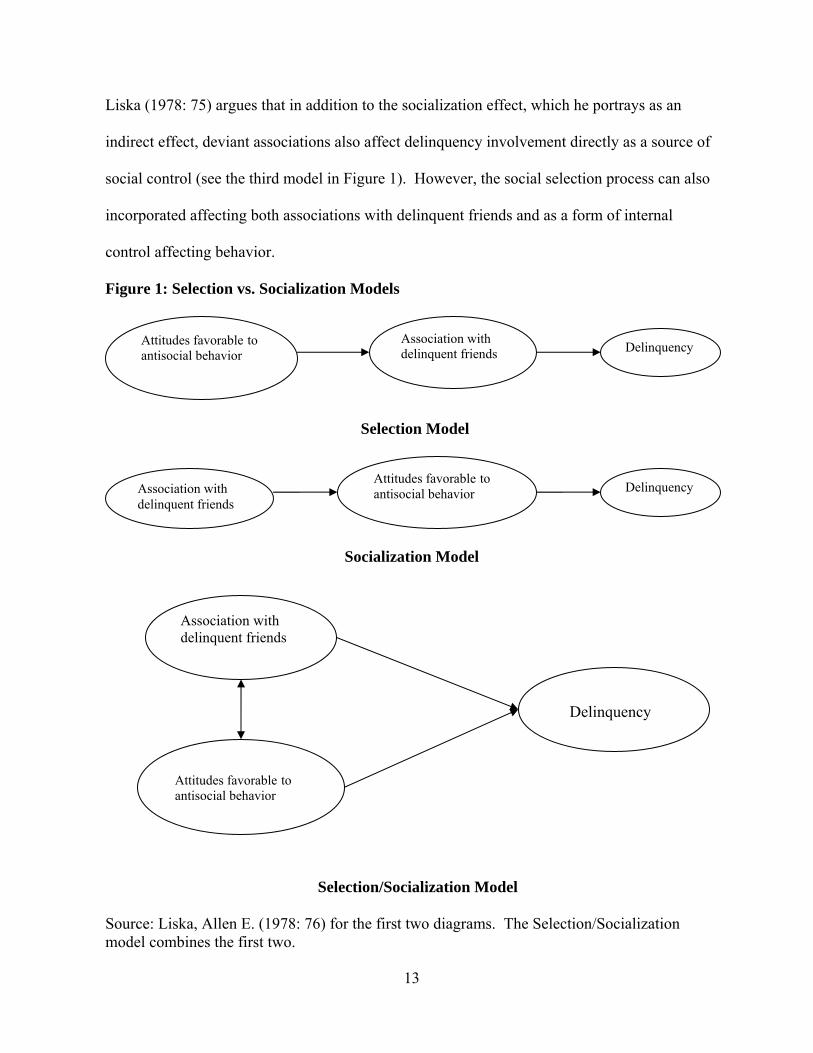
Hirschi’s theory is based on a selection model (see Figure 1 below), which suggests that
youth with weak ties to conventional others are already predisposed to antisocial behavior.
These youth are likely to associate with delinquent friends and then engage in delinquency.
Akers’ theory, on the other hand, is grounded on a socialization model (see Figure 1), which
posits that adolescents develop attitudes favorable to antisocial behavior through the
association with other delinquents; then, after acquiring such attitudes they eventually engage
in delinquency. However, it appears that selection and socialization effects are interrelated.
13
Liska (1978: 75) argues that in addition to the socialization effect, which he portrays as an
indirect effect, deviant associations also affect delinquency involvement directly as a source of
social control (see the third model in Figure 1). However, the social selection process can also
incorporated affecting both associations with delinquent friends and as a form of internal
control affecting behavior.
Figure 1: Selection vs. Socialization Models
Selection Model
Socialization Model
Selection/Socialization Model
Source: Liska, Allen E. (1978: 76) for the first two diagrams. The Selection/Socialization model combines the first two.
Association with delinquent friends
Attitudes favorable to antisocial behavior
Delinquency
Association with delinquent friends
Attitudes favorable to antisocial behavior Delinquency
Attitudes favorable to antisocial behavior
Association with delinquent friends Delinquency
14
Although Hirschi (1969) focuses on conventional relationships to explain what controls
delinquency involvement, some control scholars note the influence of delinquent peers on one’s
delinquency involvement as well as the constraints of conventional peers. To explain peer
influence, these criminologists argue that some aspects of learning theory must be integrated
with social control theory (Sarnecki 2001; see also Krohn and Massey 1980; Le Blanc and
Caplan 1993). Weak attachments to conventional as well as delinquent others make juveniles
feel they have nothing to lose, which in turn contributes to their delinquent behavior.
Although neither of these theories directly addresses the mutual effects of selection and
socialization processes, both point to human interaction, which suggests that “human
connections” or “social networks” play an important role. Further, although most youth no
doubt learn antisocial behavior through interaction with peers, their strong attachments to
conventional others presumably mitigate/constrain their delinquency. As a primary control
agent, it is inarguable that parents have a significant effect on delinquency involvement (see,
for example, Hirschi 1969; Warr 1993a). However, as social learning theorists argue, as
adolescents enter puberty they spend more time with and are influenced by their peers (see, for
example, Sutherland 1947; Akers 2000). When both effects are examined together, research so
far is still inconclusive with regard to the relative importance of each on delinquency
involvement (Warr 1993a). In other words, delinquent behavior is to some extent both learned
and constrained by an individual’s “immediate environment,” which includes parents and peers
(Scott 1991: 85). Thus, we need to know more about these immediate environments.
Social learning theory assumes that there are conflicting social norms and values in our
society, and that one side embraces conventional normative values while the other holds
alternative values. Therefore, a violation of normative values is considered deviant. However,

15
this assumption is problematic because different people belong to different groups. In other
words, what is “normative behavior” depends on one’s reference group. When people have
loyalty to antisocial others, antisocial values are considered “normative” to them and
conformity to conventional normative values can be considered deviant (Liska and Messner
1999: 64). It is necessary, then, to observe both the conventional and the antisocial network
structures in which youth are enmeshed.
Social bonding theory relies on personal perceptions rather than “facts” or actions
(Friday and Hage 1976) as opposed to behaviorists claims that “mental phenomena cannot be
part of scientific inquiry” (Liska and Messner 1999: 63). Of the four social bonds, only
“involvement” is measured by actual behavior and it refers only to time spent in conventional
activities. The quality of one’s relationship to certain individuals or groups is measured by
attachment. However, an individual’s perceived ties are not always the same as what others
perceive. That is, two-way or mutual ties between actors1 do not always exist. Thus, it is
important to look at how individuals acknowledge one another.
The social network approach incorporates others’ perceptions by using directional ties,
that is appointing and nominated ties, and in this way establish the structural connection among
participants. When examining existing ties between juveniles and others qualitatively, we need
to examine the structure of the peer group to identify directional relationships within a given
group. By doing so, we can see how juveniles are positioned within and/or across groups.
Directional, or more specifically reciprocal, relationships may help understand substance use
which is largely peer-oriented and requires others’ resources such as accessibility to substances
and knowledge of methods.
1 The term “actor” is a commonly used term in social network studies. It refers to an individual who is involved in a specific network.

16
Although the notion of friendship formation is not specifically addressed by either
social learning or control theories, understanding how adolescents are connected to and
enmeshed in a peer group may aid our understanding of the dynamics of adolescent substance
use. As noted, substance use often takes the form of co-offending. It is likely then, that one’s
peer group facilitates this behavior. It is also possible that conventional peers can constrain
youth from engaging in delinquent behavior even when delinquent peers are present or
available. As Reckless (1961) argued in his containment theory, there are push/pull factors
to/from delinquency that affect one’s behavior. It seems likely that these factors are functional
only when there is a substantial connection between juveniles, that is, how they are structurally
associated with a particular group.
Social networks can reveal how members are associated with others or where they are
located in a group and how susceptible they may be to group norms or values. How efficiently
juveniles are socialized undoubtedly depends on how they are incorporated into their friendship
network. At the same time, network variables permit examination of the selection process.
Looking at one’s location in a group over time is one way to understand both processes. In
other words, one’s choice of belonging to a certain friendship group, as well as susceptibility to
peer influence within the group is undoubtedly affected by the structure of peer groups. Thus,
by focusing on these structures, we may gain a better understanding of patterns of youthful
offending including substance use.
Patterns of Youthful Offending
According to Agnew (2009: 252), adolescents become more peer-centered as they grow
older; thus, they are more likely to be influenced by their friends and associates, and commit
offenses with friends and associates. Some evidence of this is provided by Burkett (1993) who
17
reports that the direct effect of perceived parental religiosity on one’s choice of friends and
drinking behavior decreases over time (see also Burkett 1977a). Once one chooses delinquent
friends, adolescents are influenced more by these friends than they are by others including
parents (see also, Warr 1993a).
Findings similar to the above are revealed in studies of co-offending. For example,
Weerman (2003) argues that strong attachments or emotional ties to co-offenders are not
necessary; rather, shared motivation to exchange profit may lead juveniles to co-offend. Prior
research suggests that, statistically, most offenses occur in the presence of others. Reiss, for
example, found that about 67 percent of burglary offenders and about 73 percent of robbery
offenders were co-offenders (1988: 121-122). Further, only 16.9 percent of studied juveniles
apprehended for at least one burglary during 7.5-year period were designated as solo-offenders
(1988: 123). Similarly, using official data in Sweden, Sarnecki (2001) reports that almost 60
percent of juveniles committed offenses with someone else. Although the percentage
committed by solo-offenders (41 percent) appears to be high when we focus on incidents, when
we look at offenders, the percentage of solo-offenders remains low (21 percent), consistent
with Reiss’ study (1988: 55). More recently, Warr (1996) notes that 73 percent of all
delinquent behaviors he examined were committed in a group. This was particularly true for
alcohol violations (91 percent) and all drug violations (79 percent).
In an early study focusing on group offending, Erickson (1971) found that 78 percent of
all drinking behavior and 77 percent of narcotics use were committed in group situations.
Erickson (1973) also found that over 80 percent of incidents involving drinking were
committed in groups regardless of the juveniles’ socioeconomic status. Similarly, Erickson and
Jensen (1977) revealed that about 81 to 91 percent of drinking offenses and 86 to 92 percent of

18
marijuana use offenses was committed in group situations regardless of living areas. They also
report that over 85 percent of both male and female offenders engaging in drinking and
marijuana use did so in groups.
Other empirical studies indicate that delinquent behavior is usually committed with
delinquent peers, but that in terms of socializing, delinquent youth are much like non-
delinquent youth. For example, Sarnecki (1986: 53) reports that the predominant reason for co-
offending is what he called “social motive.” That is, co-offending is “a way of socialising with
peers.” Unfortunately, it is not clear how and why these associations are formed, and why
some are socialized to group norms while others are not. Thus, whereas the characteristics of
co-offenders have been identified, the mechanism of co-offending remains largely unexplained
(Reiss 1988; Weerman 2003). This is because, with few exceptions, prior research has ignored
how group structures contribute to co-offending.
Although the number of delinquent friends is frequently used as an indicator of an
individual’s delinquency, Weerman (2003) clearly states that co-offending is different from
having delinquent acquaintances or friends. Weerman argues instead that the notion of co-
offending is useful for the analysis of social interaction and relationships among co-offenders.
He notes that co-offending includes an exchange of any rewards, either material and/or
emotional, that cannot be achieved by solo-offending. Further, social exchange is based on
needs and desires. That is, according to Weerman (2003: 404), “people base their decisions not
only on rewards but also on costs and risks…in the social exchange of co-offending. In general,
people agree to exchange goods when they expect it to be profitable enough. The same is true
for co-offending.”
19
Weerman’s proposal is relevant to understanding the difference between involvement in
networks of co-offending groups and simple association with delinquent peers or accomplice
networks as argued by Warr (1996). In other words, knowing or even associating with
delinquents is qualitatively different from actually committing delinquent acts together. In the
case of co-offending, expected rewards are gained through actual involvement in delinquency.
This suggests that juveniles who are already engaged in or are inclined to engage in delinquent
behavior select as friends those who will abide by group norms that may include engaging in
delinquency together. Thus, as already noted, knowing how an individual is enmeshed into
one’s peer group would appear, then, to be a key factor in understanding of why an individual
co-offends.
Although co-offending groups may not be gangs in the traditional sense of the term
(Sarnecki 1986), gang studies are nevertheless very informative given to the nature of
interpersonal relationships among gang members. For example, in his early study of delinquent
gangs, Thrasher (1927) found that gangs are characterized by relative stability. Youth initially
form spontaneous play-groups through their attachment to local territories and when conflicts
between groups occur they try to solve problems together. On the other hand, Yablonsky
(1973) later questioned the cohesiveness of gangs and focused on the location of members
within gangs by distinguishing between core and marginal members. He notes that even
among marginal members there are several differentiating characteristics. Because marginal
members at the fringe of the gang have no clear identification as a member, Yablonsky argues
that they can quit or shift from one gang to another. This suggests that both membership
participation and the ability to shift affiliation or drop out altogether may be structurally
defined. According to Yablonsky, juveniles who are loosely tied to a delinquent peer group are

20
less likely to engage in group activities unless they are motivated to improve their status in
group or they have any specific personal reason to commit delinquent behavior. Klein (1995)
also found that gangs in general are loosely organized although members of cliques within
gangs show high cohesiveness and tend to engage in delinquency together. Clearly, structural
connections among members affect delinquency involvement.
While gang studies provide insight into the structure of delinquent groups, Warr (1996)
examines both how such groups are structured and the characteristics of the group members.2
In his study of group structure and delinquency involvement, Warr (1996: 33) reports that
“instigators” in a delinquent group tend to be “older, more experienced, and close to other
members.” Particularly noteworthy is the finding that persons in the center of a group are
likely to facilitate the delinquent behavior of others. However, facilitating is not the same as
committing delinquent acts by themselves. Further, a very cohesive delinquent group, which in
terms of network analysis is defined as a group with high density, apparently maximizes
opportunities for members to engage in antisocial behavior.
Until recently, and except for gang research, the structure of peer groups has been
relatively ignored because prominent theories take existing networks for granted (Krohn and
Thornberry 1993: 102). An individual’s association with delinquent peers is not always
intentional or for the purpose of delinquency involvement. If an association with delinquent
peers is the result of external factors such as coercion, being a groupie, or a steady romantic
partner, an actor’s unwillingness to engage in delinquent behavior will, in turn, affect whether
and how that individual is enmeshed in and socialized within the group. On the other hand,
juveniles who chose to join a group are perhaps more likely to be connected to others and, in
2 Warr explores the character of delinquent groups excluding gangs because, he argues, they are conceptually different.
21
turn, to be socialized to the values in the group. This may be especially true for substance use.
Given the matter of access, substance use is heavily peer oriented. By focusing on friendship
network structures, we can examine the proximity between actors, which appears to be one of
the factors that affect socialization (Sutherland, 1947).
Career Offending
Career offending in general refers to lifelong criminal behavior that becomes one’s
livelihood. According to the age-crime curve, most offenders desist from antisocial activities
by the age of 30 with the peaks in the mid to late teens and early twenties (FBI 2008: Table 38).
The arrest data in the 2008 Uniform Crime Reports also show that liquor law violations as well
as drug violations peak in the 19 and 18 year old age groups respectively (2008: Table 38).
Explanations of substance use should include consideration of behavioral changes such as
entrance into, changes in the involvement level, and desistance from this behavior.
Moffitt (1993) identifies two types of offenders: Life-course-persistent (LCP) offenders
and adolescent-limited (AL) offenders, the latter of which is consistent with the age-crime
curve. LCP refers to individuals who “exhibit changing manifestations of antisocial behavior”
throughout their life course (Moffitt 1993: 679). AL refers to individuals who engage in
antisocial behavior during early adolescence, but desist sometime in their late adolescence.
Moffitt’s taxonomy for the age-crime curve suggests the need for further research over the life
course.
It is often assumed that the relationship between age and substance use over time will
exhibit a single predictable direction or trajectory. However, the behavioral trajectories of
youth typically are not singular. Following Moffitt’s lead, researchers have found more
complicated behavioral trajectories. For example, using data from a longitudinal study of

22
Pittsburgh youth, Loeber et al. (1993) identified three distinctive trajectory patterns in
offending careers: the authority conflict pathway, the covert pathway, and the overt pathway.
The authority conflict pathway is the most common and is consistent with the age-crime curve.
This pathway shows that the onset of delinquency begins at early age with stubborn behavior,
which leads to disobedience. Eventually, these adolescents tend to avoid authority figures by
staying out late, skipping school, or running away. The second two pathways show progressive
patterns. The covert pathway refers to a trajectory beginning with minor delinquent behaviors
such as shoplifting but then progress to property damage and ultimately to more serious forms
of theft. The overt pathway refers to a trajectory that begins with aggressive behaviors such as
bullying, which then escalates to more serious violent behavior. Although these three pathways
were found in their study, other evidence suggests that possible behavioral trajectories are
likely to be more complicated (see also D’Unger et al. 1998; Nagin et al. 1995). This may be
particularly true for substance use.
Using the four waves of national panel data from the Monitoring the Future survey,
Schulenberg et al. (2005) found six trajectory groups for marijuana use among adolescents
ranging from abstain (no use in the past 12 months at all four waves) to rare (infrequent
marijuana use at one or more waves), fling (no or infrequent marijuana use at waves 1and 4,
and frequent use at waves 2 and/or 3), as well as those who increased use, those who decreased
use, and some who were chronic users over time. The most common pathway is being
abstainer at all times (47 percent) followed by rare users (28 percent). Later reports using the
same data source substantiate these findings (see Johnston et al. 2007).
According to Sampson and Laub (1993: 2003; see also Laub and Sampson 1993)
behavioral change from unconventional to conventional is often the product of institutional
23
change such as joining the military or getting married. However, as Warr points out (1998),
such institutional changes do not change one’s behavior directly or do not necessarily come
first. Rather, one’s already altered behavior may bring institutional changes through relational
changes. For example, according to Sampson and Laub (1993: 2003) marriage can be a reason
for desistance from antisocial behavior. On the other hand, Warr (1998) argues that we should
consider marriage as a process in one’s life course rather than one single positive transition
point. He found that the effect of getting married on criminal behavior is largely diminished
when peer influence is held constant (202). Instead, he argues, changes in friendships before
marriage seem to explain the effect of marriage on desistance (204). Warr suggests alternative
arguments that challenge the general effect of marriage on desistence: delinquents who cease
their antisocial behaviors become more attractive as potential mates (210).
Friendship networks may contribute to these changes in behavior over time. Prior
research suggests that over time substance use often progresses through different
developmental stages. For example, Maggs and Hurrelmann (1998) examine adolescent
substance use focusing on peer relations. They include measures of the respondents’ perceived
peer group closeness and perceived position in the peer group as relational variables. Perceived
peer group closeness is positively correlated with substance use only among students who are
in higher grades (ninth and tenth), whereas perceived central position is positively correlated
with substance use among adolescents who are in middle grades (eighth and ninth). In addition,
their findings reveal that among eighth to tenth graders substance use is associated with an
increase in frequency of peer involvement whereas among tenth graders substance use is
associated with an increase in perceived peer group closeness. This suggests that adolescents’
willingness to be a part of groups, affects substance use.

24
Later, in their four-wave panel study of adolescent problem behaviors such as substance
use, Wiesner and Windle (2004) reveal that individuals show that adolescents can be classified
into distinct offending patterns resulting from changes in interaction with different types of
reference groups. Although it is almost impossible to follow the life histories of large numbers
of subjects, we can focus on certain life stage periods and conduct qualitative research to
understand whether friendships or changes in friendships affect substance use, or whether one’s
tendency to choose certain groups or one’s position in a group affects substance use.
Another example is found in the landmark study of the careers of drug smugglers by
Adler and Adler (1983). They provide an understanding of the possible role of peer networks
in their explaining of why dealers do not desist from their business. Although there are surface
factors such as resistance to giving up a hedonistic life style, they found that the social network
of underworld dealers is the strongest reason for their persistent drug dealing. Clearly, old
social networks keep pulling dealers back. Although Adler and Adler are not entirely clear on
how this social network is organized and how it affects the criminal behavior of dealers, they
do note that dealers who are already deep into the business are no longer capable of
withdrawing from the drug world. In other words, the social networks of drug smugglers are
too strong and supersede any conventional networks they may have. This study informs us that
social networks can affect one’s behavior over time and suggests the need to incorporate
network variables into the analyses.
Past studies have identified how friendship networks influence the development of
substance use. Using a three-wave panel of Ohio youth in a state-level correctional facility,
Schroeder et al. (2007) classify subjects into three groups: “desisters” who were free from
serious and/or frequent offenses and were not incarcerated during the two follow-up periods;

25
“persisters” who exhibited serious and/or frequent offending patterns and/or were incarcerated
during both follow-up periods; and, those in an “unstable” group categorized as “desisters” at
the first follow-up period but “persisters” at the second follow-up period. They report a strong
relationship between substance use and peer’s engagement in criminal activity. They also note
that when “persisters” are compared to “desisters,” friends’ criminal acts significantly lowered
the odds of desistance from use over time. This suggests that continued association with
deviant friends reduces exposure to conventional others and values that might alter their
behavior.
Clearly, individuals may not behave in the same manner throughout life. That is, they
can adopt or abolish certain values in their life and change their behavior in a manner consistent
with their “new” value system as it develops through peer association. Some are involved in
delinquency at an early age, quit offending for a period of time and then go back to offending
while others exhibit different patterns such as progressive involvement in illicit activities (see
Hawkins and Weis 1985; Loeber and LeBlanc 1990; Laub and Sampson 1993; Sampson and
Laub 1993; Catalano and Hawkins 1996; Loeber 1996; Loeber et al. 1998; etc).
Past research such as that by Garnier and Stein (2002) supports the notion that peers
exert a signification influence on initial substance use. If, as Akers claims (for example, 1998,
2000), human beings can learn and adapt conventional behavior, it seems reasonable to apply
this notion to the desistance process as well. Mere acquaintances are unlikely to affect one’s
attitude toward substance use, provide an opportunity to imitate others’ behavior, or receive
differential reinforcement. In other words, mere acquaintances are less likely to either facilitate
or constrain one’s behavior. As noted by Sutherland (1947), how we learn is weighted by
priority, duration, frequency, and intensity of one’s associations. This again suggests that we

26
should pay attention to how individuals are enmeshed into a social group. This leads us to
develop the core notion that network characteristics such as structural proximity may affect
antisocial behavior over the life course.
Empirical Studies using Social Network Analysis
Some recent research suggests that social networks provide a useful organizing concept
to bridge the theoretical concerns addressed above by focusing on identifiable relational ties or
relationships among actors within certain groups (Fischer 1977: 24). The social network
approach views actors as active subjects with choices rather than as passive objects (28-29).
Fleisher (2002: 200) argues that the social network analysis is a method of “describing and
analyzing webs of social relations.” The focus is on dynamic human interaction. Unlike
traditional delinquency studies, with the possible exception of gang studies, the social network
approach focuses on individuals as members of specific groups and how those groups are
structured.
A social network is often represented by a sociogram in which actors are dots and the
ties between them are expressed by lines. Since researchers deal with relational ties, the data
must be collected within small groups of people on a non-random basis. Graphic descriptions,
from simple sociograms to more complicated descriptions, may be useful to our understanding
of interpersonal connections within groups by measuring links (ties) among actors. In this way
they illustrate how groups are formed and how the individuals within them are connected. The
social network approach can be used in both quantitative/statistical and qualitative/descriptive
analyses.
According to Krohn (1986: S82-S83), a primary assumption underlying this approach is
that “a social network constrains individual behavior…and the probability of behavior
27
consistent with the continuance of their network relationships will increase.” That is, what
facilitates or restrains one’s behavior is not just whom one knows, but how one is related to
others in the network. Social network variables consistent with social learning and control
theories allow us to examine the effect peer relationships have on substance use.
In a subsequent study, Krohn et al. (1988) examine the relationship between specific
characteristics in adolescent social network structures and cigarette smoking to test Friday and
Hage’s (1976) notion that “role overlap” accounts for much delinquent behavior. Friday and
Hage (1976: 355) argue that the number of opportunities to be socialized to conform to social
norms will depend on the types of relationships an actor has. Krohn et al. (1988) hypothesize
that greater multiplexity, that is involvement in multiple groups with different social roles
between any two actors in different social contexts, constrains a member’s behavior within
given groups because his/her antisocial behavior is more likely to be detected. Krohn et al.
report that joint participation in conventional activities with peers or parents reduces the risk of
cigarette smoking. Their findings support the notion that network multiplexity may constrain
an actor’s antisocial behavior. Similarly, Burkett (1977a, b; see also Burkett and Jensen 1975)
reports that isolation from conventional activities may lead to heavy involvement in alcohol
and drug use. However, it is highly unlikely that individuals belong to only one institution,
organization, or group. As a counter argument, simply joining multiple groups will not in itself
exert much control over one’s behavior. Rather, how well individuals are recognized by other
members within those groups is likely to be more important. Nonetheless, Thornberry et al.
(2003: 15) later declare that a network perspective assumes that “all social networks constrain
the behavior of their participants to some extent depending on the structure of the social
network.”
28
Although Krohn et al. (1988) provide some supportive evidence for multiplexity; their
study is not limitation-free. First, certainly one’s association with groups may change over
time. However, whether such changes in association affects antisocial behavior or the tendency
of an individual to take a similar position in a new group regardless of changes in friendship is
not known, which suggests the need for longitudinal data. Second, the quality of relationships,
that is, mutual acknowledgements within groups, is often overlooked. In other words, joining
multiple groups does not determine the quality of relationship. Thus, the nature of each
association within and/or across groups should be examined as well as how joint participation
in conventional activity impacts one’s behavior.
While there is evidence that multiplexity within friendship networks plays an important
role in substance use, another network characteristic, that is, the cohesiveness of groups, must
be examined (see also, Baeveldt and Snijders 1994 and Haynie 2001). For example, using data
from the Rochester Youth Development Study, Krohn and Thornberry (1993) examine the
effects of network characteristics on the stability in alcohol and marijuana use. Although they
find that cohesiveness does not show any significant difference between drug users and non-
users, different levels of cohesiveness appear to be related to race/ethnicity. They find that
both African American and Hispanic alcohol and marijuana users are likely to be in more
intimate relationships than are non-users. This suggests that within certain racial/ethnic groups
substance user groups are relatively cohesive, and therefore provide greater opportunities for
involvement in substance use. Determining levels of cohesiveness may be a key to
understanding substance use that often takes the form of co-offending.
Fleisher’s (2000) ethnographic research in Kansas City is based on a social network
approach. This study documents how gang members get involved in delinquency. His findings

29
suggest that youth engaged in serious delinquency are more likely to be located in the center of
the gangs. The closer and stronger the ties between members, especially among core members,
the more troubles in any way they have in life. This is consistent with Warr’s (1996) findings
that with the exception of assault the instigators of offenses are more likely to have committed
prior offenses than are joiners.
Haynie (2001) reports that among popular youth, peer’s delinquency involvement is
strongly associated with one’s own delinquency. While instigators tend to be in the center of a
group and more actively engage in delinquency, the questions remain about who initiates
crime/delinquency. Haynie’s findings suggest that the more popular an individual is, the more
opportunities for antisocial behavior they have and the more likely they are to be influenced by
their peers. Although there is a measurement flaw in her research3 popularity is an important
network characteristic that needs further examination.
Using National Youth Survey data, Wright and Cullen (2004: 186) report that
respondents who obtained “new sets of peers” at one’s workplace are more likely to disrupt old
delinquent relationships and to alter their past antisocial behavior through newly formed
associations. The change in social network alters one’s delinquent behavior and prevents future
offending because offending would risk losing the new relationships. Unfortunately, the
quality of relationships between subjects and their prosocial coworkers is not taken into
account. In other words, a mere change in association may not be enough to convince the actor
to quit antisocial behavior. How they are connected, that is, the quality of their relationships
should be considered.
3 The number of appointments from others as a friend is not standardized by the number of group members. Because the maximum appointment is conditioned by the group size, we have to adjust the number of appointments by the group size.

30
As noted, Weerman (2003) and Warr (1996) claim that mere association with
delinquent peers is not adequate to explain co-offending. Rather, how juveniles are tied
together in a friendship group and how they are enmeshed into the group may explain co-
offending. Also, Fleisher (2000) reports that gang members who are located in the center of the
group are more likely to commit offenses. In addition, a leader, who tends to be in the center of
a group, commits more offenses and those who commit recognizable amount of offenses would
gain a position near center. As already noted above, a popular person may have opportunities
for delinquent activities brought to their attention by other members.
As already alluded to, another factor that may affect offending is group cohesion. As
Klein (1971) observes, less cohesive gangs are more likely to engage in a greater variety of
delinquent behaviors, whereas more specialized gangs are more likely to be characterized by
group solidarity as Thrasher (1927) described. Also, Warr (1996: 33) reports that juveniles
commonly “belong to multiple delinquent groups over their careers and they change their
accomplices frequently,” which would suggest that such groups tend not to be terribly cohesive.
Given this, the evidence that group cohesiveness is a major factor regarding engagement in
delinquent activities is inconclusive. If juveniles constantly “drift” (Matza 1964) between the
conventional and unconventional, identifying how they become enmeshed in a certain group at
the point of offending may help us understand the nature and role of these groups.
The above empirical research suggests three issues regarding social networks: 1) mere
association with delinquent peers is not enough to explain either individual behavior or co-
offending; 2) core members who are located close to the center of a delinquent group appear to
be more likely to commit delinquent behavior; and 3) although there is conflicting support for
the notion, it appears that individuals in cohesive groups are less likely to engage in delinquent

31
behavior. With regard to the latter, social control theory seems to suggest that groups in which
members are strongly attached to one another are likely to support conventional norms. Less
cohesive groups may facilitate delinquency or substance use given weak conventional controls
that are likely to exist.
In addition to the above, it appears from the review of the literature that some attention
should be paid to diversity within groups. Early on, adolescents tend to develop their
friendship networks in school and are likely to choose same-sex friends. Depending upon the
composition of the school or neighborhood, they may also choose friends in terms of
racial/ethnic similarities and differences (see, for example, Cairns and Cairns 1994). If we
assume that groups that are heterogeneous in terms of race/ethnicity are likely to be less
cohesive and therefore exert weak conventional controls, then members of such groups are
more likely to engage in substance use. In other words, members of such groups may enjoy
more freedom in their behavior, which may increase the likelihood of substance involvement.
As control theory suggests, members of less cohesive groups may not be subject to
conventional controls that would prohibit substance use.
I should also note that Cairns and Cairns (1994: 109) report that during mid-
adolescence, social groups tend to be homogeneous with regard to age, gender, and race. A
major property of school systems is segregation by age. Thus, as long as individuals participate
in traditional school systems, age similarities in one’s peer group are likely to exist over time
all other things being equal. Regarding gender, such homogeneity diminishes to some extent
as youth grow older, but it is likely to remain a strong factor in terms of choice of friends
during adolescence. However, compared to gender, racial homogeneity appears to increase as
youth advance through the adolescent years. Cairns and Cairns (109) argue that adolescents

32
compared to young children are aware of differences, are under strong pressure to choose
friends who are similar to themselves, and are more likely to have opportunities to achieve
similarities as a function of development, and this may extend to race/ethnicity. Although they
report lower incidence of substance use among African Americans, how this affects substance
use in the context of diversity in groups remains to be seen.
Finally, past theories and research suggest that how an individual is associated with a
group may affect delinquency involvement, and a change in relationships over time may alter
one’s behavioral trajectory. The notion of social networks appears to be important to
understanding substance use at any stage of one’s life. In the following chapter, several
hypotheses derived from social learning and control theories and past research are presented.

33
CHAPTER THREE
HYPOTHESES
As noted in the previous chapter, the majority of youth engaged in delinquent behaviors
including substance uses are involved with other youth engaged in similar behaviors. Social
learning theory suggests that youth involved in friendship groups that include “delinquent”
peers are socialized by those peers, and as a result, come to share definitions favorable to illegal
behavior including substance use and to engage in behaviors consistent with those attitudes
(Akers, 1998: 2000). Some extend this idea to include consideration of co-offending, which
according to Sarnecki (1986:53) represents “a way of socialising with peers.”
On the other hand, social control or bonding theory (Hirschi 1969) suggests that youth
with weak bonds to conventional others and who do not maintain strong beliefs in the moral
validity of the law are likely to select as friends those who drink or use drugs. However,
choosing the “wrong crowd” does not necessarily mean that juveniles will actually engage in
substance use. Whether they do or not engage in these behaviors is likely to depend on how
they are enmeshed in or connected to a group of substance users. In other words, the strength
of peer group socialization effects and the likelihood that youth will engage in these behaviors
will depend upon where an individual is located within a group, that is, how the actor is
recognized by his/her peers and where they locate themselves.
Although social learning and control theories tend to ignore these structural and
organizational aspects of peer groups, it has been suggested by some that criminologists should
direct their attention to the relationship between the structure of social networks and the
processes of social selection and socialization. Cairns and Cairns (1994), for example, aptly

34
describe how social networks function, and emphasize the importance of examining selection
and socialization effects together:
Within the clusters of adolescence, strong reciprocal forces operate on all members toward conformity...A systematic account of social clusters and friendship must take into account the powerful effects of reciprocal influence demonstrated in experimental studies and observational analyses. The message from these investigations is that reciprocal interactions lead to high levels of behavioral and attitudinal similarity, regardless of the initial status of the people involved. The evidence on adolescent group dynamics strongly points to the operation of both differential selection factors and reciprocal influences (1994: 128-9) [Emphasis added].
Here substance use will be examined using social network variables that incorporate both
selection and socialization effects. By doing so, I hope to determine whether certain
characteristics of friendship groups render juveniles more or less susceptible to substance use.
Coleman (1961) argues that over several decades the school has become a major
institution affecting adolescent behavior. Because most youth spend considerable time in
school with people their own age, it makes sense to examine school-based friendship groups.
Polk and Schafer (1972), like Coleman note that a major characteristic of school is “the age
segregation and cloistering” that occurs in that context, and that the “high school has come to
dominate the life of the adolescents and many of the free-time activities of the student are also
school-based.” (13) As Sutherland (1947) proposed several decades ago, how juveniles learn
certain values is weighted by four factors: frequency, duration, priority, and intensity. With
regard to their peers, these four factors are likely to be affected by their involvement in the
school system. Given the nature of schools, youth spend considerable time in structural
proximity to each other through both formal and informal activities. The school is the source
of various social evaluations that often affect their choice of friends. Thus, youth tend to
become involved with friendship groups that develop within the school they attend. An

35
individual’s susceptibility to peer influence is likely to depend on one’s position in one or more
of the many groups that exist within the school context.
Whether one is centrally or marginally connected to a friendship group or how close
one is to other members is also likely to impact one’s involvement in both conventional and
“illegal” behavior. In other words, one’s position in a social network is expected to affect one’s
use or non-use of alcohol and/or other drugs and if the former the level of one’s use. However,
one’s involvement in friendship groups is also influenced by other factors. For example, a key
institution affecting one’s friendships and behavior is the family. Parents in particular exert
considerable and typically conventional control over adolescent behavior. Attachment to
parents helps shape adolescent friendship networks by influencing the selection of friends who,
in turn, influence substance use. If true, the effects of the network characteristics should
become stronger when the effect of attachment to parents is held constant. Furthermore, given
the increased frequency of involvement, the importance attached to various activities and
individuals as well as the intensity of school-based networks, it is expected that this influence
will endure over time as other sources of control such as attachment to parents diminish over
time relative to the influence of peers with whom they become increasingly involved.
Warr (2002: 130) notes that most delinquency theories focus primarily on individual
differences rather than group differences. Group characteristics are rarely paid attention to
when we try to understand individual differences for antisocial behavior (see also Krohn and
Thornberry, 1993; Fleisher, 2000; Haynie, 2001). It seems likely that social network variables
such as Centrality, Prestige, Density, and Heterogeneity can be used to explain the level of
substance use. From a structural viewpoint, Centrality, that is, an actor’s perception of his/her
position in a group and his/her Prestige or popularity within a friendship group are argued to be
36
predictors of substance use to the extent that they provide increased opportunities to engage in
such behaviors. According to Warr (1996), location in the center of a group may facilitate
engagement in substance use.
On the other hand, Density or cohesiveness may be expected as a constraining factor.
That is, from control perspective, cohesiveness may produce conformity to normative behavior.
In other words, in cohesive groups, members are likely to monitor others’ behavior not to
deviate. However, some may argue that cohesion in groups facilitate antisocial behavior
because cohesiveness must be present for secrecy when adolescents engage in illegal behavior.
Thus, when a peer group is cohesive enough to show loyalty to group norms, substance use is
likely to occur. Although past gang research at least suggests the opposite consequences of
Density (see Thrasher 1927; Klein 1995), I argue that substance use is less likely to occur in
cohesive groups.
Two types of directional ties are used to quantify an actor’s location in a group: out-
degree and in-degree. Out-degree refers to an actor nomination of others as friends, while in-
degree refers to actor being appointed as a friend by another actor. Centrality is defined in
terms of out-degree, that is, the number times an actor nominates others as friends. Centrality
refers to an actor’s “activeness” or willingness to be a part of one friendship group rather than
another.
Prestige measures one’s popularity. Using network terminology, popularity is called
Prestige, which refers to appointed ties from others, that is, in-degree. An offending event
within a group context suggests that availability of opportunity to engage in substance use is a
key variable. In other words, a popular actor in a given group is likely to be informed and
invited to participate in offending opportunities if they occur.

37
Density refers to the cohesiveness of a group. Within the context of gang studies,
Thrasher (1927) suggests that when gangs encounter external conflicts, they exhibit high
cohesiveness or solidarity in order to resolve the conflicts. Therefore group members are likely
to expect similar behaviors from one another in the future. On the other hand, there is at least
some evidence which suggests that gang members are loosely connected to one another (Klein
1995). Thus, in some cases a lack of group cohesion may increase the likelihood that group
members will engage in antisocial behavior including substance use.
Apart from gang studies, Krohn (1986: S82-83) found that social networks typically
constrain one’s behavior. In a subsequent study, Krohn et al. (1988) examined how
multiplexity may produce conformity. Their findings suggest that one’s antisocial behavior is
easily detected if an individual is a member of multiple groups that constrain one’s behavior.
They also note that as constraints decrease, the probability that people will engage in
unacceptable behaviors increases. However, although it is common that individuals belong to
multiple groups, institutions, or organizations, simply joining multiple groups is unlikely to
produce conformity. If no one recognizes an individual or cares about his/her behavior, one
might question whether group participation serves as a constraining factor. Multiplexity as
identified by Kohn et al. (1988) may constrain individuals’ antisocial behavior only when
members recognize each other within such groups.
If this is the case, recognition by other group members or Density is expected to
produce conformity to normative behaviors of the group. Consistent with findings by Krohn
(1986) and Krohn et al. (1988), Haynie (2001) reports that high cohesiveness in a group will
reduce the level of delinquency involvement. However, Krohn and Thornberry (1993) report
that cohesiveness among African American and Hispanic alcohol and marijuana users is higher

38
than what is found for other racial/ethnic user groups. Since substance use is a prohibited
behavior, loyalty to a membership group or secrecy may be essential for these youth. Although
cohesiveness may serve as a monitoring function within some groups thus controlling
members’ antisocial behavior, it may allow higher levels of substance use in groups in which it
is acceptable behavior. Although findings from past research are mixed, it is expected that
greater Density will be negatively associated with substance use.
Given the above, it seems clear that Heterogeneity or diversity in a group, may affect
one’s substance use though perhaps indirectly. As mentioned in the previous chapter,
adolescents may choose friends in terms of racial/ethnic similarities and differences depending
upon the composition of the school or neighborhood (see, for example, Cairns and Cairns 1994).
Control theory suggests that members of less cohesive groups may not be exposed to consistent
conventional controls that would prohibit substance use. Therefore, in general, it is expected
that racially/ethnically heterogeneous groups will be less cohesive and therefore less
constraining in terms of substance use.
In addition to the network variables I also examine whether the effect of attachment to
parents plays a significant role on adolescent substance use. Haynie and Osgood (2005) report
that while youth are more likely to engage in delinquent behaviors if their friends are highly
delinquent, youth who spend considerable unsupervised time with friends are more likely to
engage in delinquent behaviors even after controlling for peer delinquency. Further, as Warr’s
(1993a) finding that parental attachment has little effect on delinquency involvement once
adolescents are already exposed to delinquent peers, suggests that for some youth parental
control is often limited to the time period before adolescents start to associate with their peers.
Past research suggests that parents may be a strong contender to the influence of peers, but that
39
this effect appears to be conditional. I argue that peer influence is determined by where an
individual is located in a peer group. Here, I examine whether one’s structural position in a
friendship group remains when controlling for the effect of attachment to parents. Thus, when
attachment to parents is held constant, the more likely it is that one will be influenced by peers
in terms of peer group Centrality, Prestige, and Density and that these youth are more likely to
be involved in substance use.
The first set of hypotheses focuses on immediate or short-term network effects. The
second set focuses on long-term effect of early network variables.
H1-a: The greater the Centrality of an actor’s location in his/her peer group, the greater
the likelihood the actor will engage in substance use.
H1-b: The greater an actor’s Prestige in his/her peer group, the greater the likelihood
the actor will engage in substance use.
H1-c: The greater the group Density of an actor’s peer group, the less the likelihood that
the actor will engage in substance use.
H1-d: The greater the racial/ethnic Heterogeneity of a group, the greater the likelihood
of substance use.
H1-e: The effects of Centrality, Prestige, Density, and Heterogeneity on substance use
will be stronger when the attachment to parents is held constant.
Although the strong correlation between early substance use and later use is often noted,
the long-term effects of friendship networks on substance use have not been systematically
examined. As noted earlier, Sutherland (1947: 7) argued associations leading to the learning of
definitions favorable to the violation of the law would vary in terms of frequency, priority,
duration, and intensity. It was also noted, particularly in reference to Coleman (1961) that
40
school-oriented peer relationships occupy a significant part of the life of adolescents (see also
Polk and Schafer 1972). Furthermore, this comes with the added element of increased
separation from adults, and perhaps most notably parents, who traditionally have been the
primary source of conventional social control with respect to youthful behavior.
Given the role of schools in the lives of adolescents, it may be argued that social
network relationships that develop from middle school through high school are likely to play a
significant role in the development of social and behavioral patterns that will impact extend at
least into early adulthood. If true, then early network relationships may help explain the strong
correlation between early and later substance use. Thus, we can expect that the social network
variables will help explain the apparent causal effect of early substance use on later use. This is
the focus of the second set of hypothesis.
H2: The effect of early alcohol and marijuana use on future alcohol, marijuana, and
other illicit/unauthorized drug use in early adulthood is attenuated by early network
variables, Centrality, Prestige, Density, and Heterogeneity.
If H2 is true, we can expect that when we control for effects of the early social network
variables the statistical relationship between early and later use will be mitigated. That is, the
early social network variables also account for later substance use.
Finally, it is often assumed that the relationship between age and the level of substance
use over time will follow a single predictable direction or trajectory. However, the behavioral
trajectories of youth typically are not singular. For example, as already noted, some past
research (see D’Unger et al. 1998; Nagin et al. 1995; Loeber et al. 1993) has identified multiple
trajectory patterns in career offending. Whether multiple and meaningful pathways exist in
terms of changes in the level of substance use among youth in this study is at this point an open

41
question. However, since alcohol is a legal for adults we can expect that with age many will
begin use and some will increase the level of use. On the other hand, because marijuana use is
illegal for both youth and adults it is expected that the number of users will decrease as youth
move into adulthood and have more to lose by getting caught. Thus, different trajectory
patterns between alcohol and marijuana use are expected.
H3: Over time the trajectory for alcohol use will show an increase in drinking behavior,
while that for marijuana use will show a decrease.
In summary, the focus of this study is on how the network variables, Centrality,
Prestige, Density, and Heterogeneity, which incorporate both selection and socialization effects,
influence substance use. Because most youth attend school, friendships developed there are
perhaps particularly important because they spend considerable time in structural proximity to
one another in formal or informal activities. Therefore, these hypotheses will be tested using
data from a study of in-school youth. In the following chapter, the data will be described along
with the measurement of the variables and the analytical strategy to be used.
42
CHAPTER FOUR
METHODS
Introduction
The central question for this research is: How do peer network characteristics affect
substance use among adolescents? The selection of friendship groups and an actor’s structural
position in a group are used to explain the relationship between peer involvement and substance
use. This study includes two separate analyses: a quantitative analysis and a case study. In the
quantitative analysis, I examine the relationships between a set of peer network characteristics
and adolescent substance use. I then focus on identifiable friendship groups within one school
to illustrate the results of the quantitative study. In the case study, I examine how individuals
are connected and determine the level of substance use among and within peer groups. The
case study is performed to visualize the interrelationships among peers and the level of
substance use and to observe structural equivalence among them that is not accomplished by
the quantitative study. The visual results revealed in sociometric diagrams allow us to
understand of the association between one’s structural position and substance use. The data,
methods, and measurement are described below.
Study Design and Sample
This study uses data from the National Longitudinal Study of Adolescent Health (Add
Health),4 which focuses on adolescent health and risk-taking behaviors in the context of social
networks such as families, friends and other peers, schools, neighborhoods, and communities.
The Add Health study was initiated in 1994 “under a grant from the National institute of Child
4 The Add Health study was designed by J. Richard Udry (Carolina Population Center, UNC-Chapel Hill), Peter S. Bearman (Department of Sociology, Columbia University) and Kathleen Mullan Harris (Department of Sociology, and Carolina Population Center Faculty Fellow, UNC-Chapel Hill).

43
Health and Human Development (NICHD) with co-funding from 17 other federal agencies (see
Harris et al. 2009).” The study initially involved youth enrolled in grades 7-12 in a nationally
representative sample of 145 schools. Waves I and II were conducted in 1994-1995 and 1996
respectively and explored factors that influence adolescent behavior. These factors included
personal characteristics, comprehensive information about families and friends, romantic
relationships, peer group involvement, and school, neighborhood, and community
characteristics. Wave III consisted of interviews conducted in 2001-2002 when the original
respondents were between ages 18 and 26.
The Wave I data consist of responses to a self-administered in-school survey completed
by approximately 90,000 students enrolled in grades 7 through 12 with a high school
participation response rate of more than 70 percent. Slightly over 20,000 students were then
selected from the rosters of the participating schools for a second phase of Wave I. This
involved an in-home interview with the respondents and their parents. In the home-interviews,
students were asked questions about sensitive issues such as sexual orientation and criminal
activities that were not included on the in-school questionnaire. Friendship network data were
collected as a part of the in-school survey. Respondents were asked to nominate up to five
male and female friends. Valid nominations are friends whose name appeared on the
respondent’s school roster. The Wave II data consist of an in-home interview with 14,738
students who participated in Wave I.5 Follow up data were gathered in 2001-2002 with 15,170
respondents6 participating in the Wave III in-home interview.
5 For details, consult with UNC Carolina Population Center: Add Health website—study design. 6 A fourth in-home interview (Wave IV) was conducted using a nationally representative sample of over 20,000 adolescents who were first interviewed in Wave I. However, as of September 2009 the Wave IV data had not been released.

44
Embedded within these cross-sectional surveys is a three-wave panel study design that
included students who participated in both the in-school survey and the in-home interviews at
all three time periods (N=8,503). From this number, 334 respondents whose ages7 were not
reported or were younger than 13 and older than 18 at Wave I, were excluded to include the
common age range at junior high and high school. In addition, 84 respondents who did not
identify their race/ethnicity were dropped. The resulting sample includes 8,085 respondents
from 132 schools.8
Identification of a school to be selected for the case study was limited to schools in
which the entire student body participated in the in-home interview. The questionnaire
completed by school administrators was used to identify a “saturated sample.”9 This saturated
sample allows us to identify friendship groups within a given school. Sixteen schools met the
criteria for a “saturated school.” Although all students from these schools were interviewed at
home, not all students participated in the in-school survey in which the network questions were
asked, and some did not participate in the Wave II in-home interview. In addition, ten schools
in which less than 70 percent of the students participated in the in-school survey during Wave I
and/or Wave II interview were eventually dropped because most of the network and/or
substance use information was not available. The number of respondents in the five schools in
which more than 70% of students participated in all of the in-school surveys and Wave I and
Wave II in-home interviews, were 20, 43, 53, 55, 61, and 161, respectively.
7 Age is calculated based on the date the students were interviewed. Some discrepancies in self-reported sex are corrected. 8 In addition to the above, a picture vocabulary test was also given to the respondents, and spatial data that identify the respondents’ household in a community were included in the Wave I data. The picture vocabulary test, the interviews with the parents, and the spatial data are not used in the current study. 9 School information was collected from school administrators. One question asked whether “all students at this school were selected for the In-Home Interview” (Add Health School Information Codebook). Responses to this question were used to identify saturated schools.

45
Because the purpose of case study is to provide a visual understanding of the
relationship between friendship connections and substance use, a school with sufficient data in
terms of friendship networks and substance use but small enough to diagram was selected. The
sample school consists of 61 respondents. Consistent with the quantitative sample, the age
range is limited to the initial 13 to 18 year old group. Although the quantitative and case study
samples are similar in terms of age and sex distributions there is, unfortunately, almost no
racial variation in the case study sample (see Tables 3 and 4).
Dependent Variables
Three types of substance use and two types of alcohol related problems are examined:
Frequency of alcohol and marijuana use reported at Waves II and III; other drug use at Wave
III; and binge drinking and problems caused by drinking reported at Wave III (see Appendix A).
Frequency of alcohol use is measured by the following question: “During the past 12
months, on how many days did you drink alcohol?”10 Drinking under parental supervision or
having just a sip is not counted as experience. Responses are collapsed into seven categories
ranging from “Never” (0) to “Every day or almost every day” (6).
During Wave II, marijuana use is measured by the following question: “Since the last
interview, how many times have you used marijuana?” Frequency of marijuana use is
converted into three categories: “Never” (0), “1-10 times” (1), and “More than 11 times” (2).
At Wave III, marijuana use is measured by the question: “In the past year, have you used
marijuana?” The response alternatives were: Yes (1) or No (0). Unfortunately, given this
change in wording, the variation in the level of marijuana use at Wave III is different from that
at Wave II.
10 All questions presented in the text are directly cited from the codebooks.
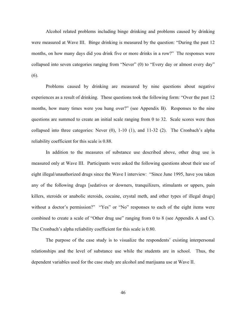
46
Alcohol related problems including binge drinking and problems caused by drinking
were measured at Wave III. Binge drinking is measured by the question: “During the past 12
months, on how many days did you drink five or more drinks in a row?” The responses were
collapsed into seven categories ranging from “Never” (0) to “Every day or almost every day”
(6).
Problems caused by drinking are measured by nine questions about negative
experiences as a result of drinking. These questions took the following form: “Over the past 12
months, how many times were you hung over?” (see Appendix B). Responses to the nine
questions are summed to create an initial scale ranging from 0 to 32. Scale scores were then
collapsed into three categories: Never (0), 1-10 (1), and 11-32 (2). The Cronbach’s alpha
reliability coefficient for this scale is 0.88.
In addition to the measures of substance use described above, other drug use is
measured only at Wave III. Participants were asked the following questions about their use of
eight illegal/unauthorized drugs since the Wave I interview: “Since June 1995, have you taken
any of the following drugs [sedatives or downers, tranquilizers, stimulants or uppers, pain
killers, steroids or anabolic steroids, cocaine, crystal meth, and other types of illegal drugs]
without a doctor’s permission?” “Yes” or “No” responses to each of the eight items were
combined to create a scale of “Other drug use” ranging from 0 to 8 (see Appendix A and C).
The Cronbach’s alpha reliability coefficient for this scale is 0.80.
The purpose of the case study is to visualize the respondents’ existing interpersonal
relationships and the level of substance use while the students are in school. Thus, the
dependent variables used for the case study are alcohol and marijuana use at Wave II.

47
Independent Variables
The independent variables include the network characteristics, which refer to how
individuals are enmeshed into friendship groups. In addition, the respondents’ attachment to
parents is also included as an independent variable. Because I am examining future substance
use, the independent variables must be measured prior to the dependent variables (see Elliott
and Voss, 1974; Farrington, 1986; Liska and Messner, 1999). Therefore, all independent
variables are measured at Wave I.
Four key network variables are used to explain substance use. These include: Centrality,
Density, Prestige, and Heterogeneity. Unfortunately, there is little agreement on terminology
and definition among network scholars. Therefore, Wasserman and Faust’s (1994) terminology
and analytical orientation are used here.
The key network element, Degree indicates the extent to which an actor is related to
others in his/her social network and is measured by the number of non-directional ties an actor
possesses. Degree can be differentiated into two types of directional ties: 1) In-degree, which
refers to the number of nominations as a friend received from others; and, 2) Out-degree, which
refers to the number of nominations as a friend that the actor directs to others. As noted,
Degree itself is non-directional, which means that mutual nominations between two actors are
not necessary. However, because directional ties suggest a stronger link between two actors
than does a one-way connection, directional ties are used to measure the four network variables.
Centrality assumes that an actor who is in the center of the network is active,
independent, and has options from which to choose in terms of behavior. Therefore, Centrality
is measured using the actor’s nomination of others, that is, Out-degree standardized by all
possible nominations within a group. Centrality is quantified by the following formula:

48
CENTRALITY = Out-degree
g-1
Where g = The number of group members or group size11
Prestige refers to how popular and/or important an actor is within a given network.
This is measured by the proportion of appointed ties or In-degree to the maximum number of
possible appointed ties. For example, the maximum number of possible appointed ties in a
group of ten is nine. Thus, an individual who is appointed as a friend from nine members the
actor is considered very popular in the group. Prestige is calculated by the following formula:
PRESTIGE = In-degree g-1
Where g = The number of group members or group size
Density refers to the cohesiveness of a group and is defined as the proportion of the
number of existing ties in a group to all possible ties in that group. Density is calculated by the
following formula:
DENSITY = The sum of total send- and receive-network12 g * (g -1)
Where g = The number of group members or group size
Where g * (g -1) = The number of possible ties
Lastly, Heterogeneity refers to how diverse a group is. Here Heterogeneity in a group is
based on the racial/ethnic attributes of the group members. Heterogeneity is a group-based
variable quantified by the following formula:
Where A = the categorical attribute: race
Ak = the number of nodes with trait k in the ego network en = the number of nodes in the ego network with valid data on A n = the total number of traits of A represented in the ego network
11 Group size can be measured by several ways: based on nominating ties, appointed ties, and nominating-appointed (non-directional) ties. Since a group usually consists of both nominating ties and appointed ties, group size in this study is determined by both nominating and appointed ties. 12 This refers to directional ties.
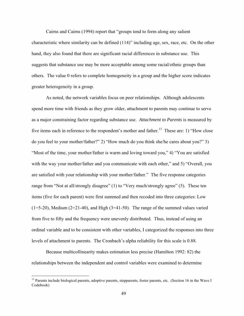
49
Cairns and Cairns (1994) report that “groups tend to form along any salient
characteristic where similarity can be defined (114)” including age, sex, race, etc. On the other
hand, they also found that there are significant racial differences in substance use. This
suggests that substance use may be more acceptable among some racial/ethnic groups than
others. The value 0 refers to complete homogeneity in a group and the higher score indicates
greater heterogeneity in a group.
As noted, the network variables focus on peer relationships. Although adolescents
spend more time with friends as they grow older, attachment to parents may continue to serve
as a major constraining factor regarding substance use. Attachment to Parents is measured by
five items each in reference to the respondent’s mother and father.13 These are: 1) “How close
do you feel to your mother/father?” 2) “How much do you think she/he cares about you?” 3)
“Most of the time, your mother/father is warm and loving toward you,” 4) “You are satisfied
with the way your mother/father and you communicate with each other,” and 5) “Overall, you
are satisfied with your relationship with your mother/father.” The five response categories
range from “Not at all/strongly disagree” (1) to “Very much/strongly agree” (5). These ten
items (five for each parent) were first summed and then recoded into three categories: Low
(1=5-20), Medium (2=21-40), and High (3=41-50). The range of the summed values varied
from five to fifty and the frequency were unevenly distributed. Thus, instead of using an
ordinal variable and to be consistent with other variables, I categorized the responses into three
levels of attachment to parents. The Cronbach’s alpha reliability for this scale is 0.88.
Because multicollinearity makes estimation less precise (Hamilton 1992: 82) the
relationships between the independent and control variables were examined to determine
13 Parents include biological parents, adoptive parents, stepparents, foster parents, etc. (Section 16 in the Wave I Codebook)
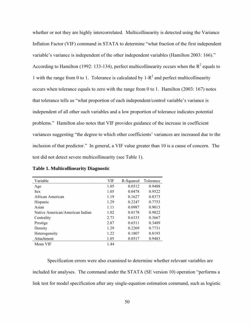
50
whether or not they are highly intercorrelated. Multicollinearity is detected using the Variance
Inflation Factor (VIF) command in STATA to determine “what fraction of the first independent
variable’s variance is independent of the other independent variables (Hamilton 2003: 166).”
According to Hamilton (1992: 133-134), perfect multicollinearity occurs when the R2 equals to
1 with the range from 0 to 1. Tolerance is calculated by 1-R2 and perfect multicollinearity
occurs when tolerance equals to zero with the range from 0 to 1. Hamilton (2003: 167) notes
that tolerance tells us “what proportion of each independent/control variable’s variance is
independent of all other such variables and a low proportion of tolerance indicates potential
problems.” Hamilton also notes that VIF provides guidance of the increase in coefficient
variances suggesting “the degree to which other coefficients’ variances are increased due to the
inclusion of that predictor.” In general, a VIF value greater than 10 is a cause of concern. The
test did not detect severe multicollinearity (see Table 1).
Table 1. Multicollinearity Diagnostic
Variable VIF R-Squared Tolerance Age 1.05 0.0512 0.9488 Sex 1.05 0.0478 0.9522 African American 1.19 0.1627 0.8373 Hispanic 1.29 0.2247 0.7753 Asian 1.11 0.0987 0.9013 Native American/American Indian 1.02 0.0178 0.9822 Centrality 2.73 0.6333 0.3667 Prestige 2.87 0.6511 0.3489 Density 1.29 0.2269 0.7731 Heterogeneity 1.22 0.1807 0.8193 Attachment 1.05 0.0517 0.9483 Mean VIF 1.44
Specification errors were also examined to determine whether relevant variables are
included for analyses. The command under the STATA (SE version 10) operation “performs a
link test for model specification after any single-equation estimation command, such as logistic

51
regression and regression.” It provides an initial diagnosis that indicates whether a model is
properly specified by the predictor variables (see Table 2). This test is run after the logit or
logistic regression is estimated. To determine whether the model in which necessary variables
are included is properly specified, the “linktest” creates two variables: the linear predicted
value (_hat) and linear predicted value squared (_hatsq). The first coefficient (_hat) must be
significant because this value reflects the significance of the model itself. The second
coefficient (_hatsq) suggests that we might omit relevant variable(s), usually interaction terms,
if the value is significant. The linear predicted value (_hatsq) indicates that the linktest failed
to reject the assumption that the model is properly specified without removing any variables.
Thus, specification error is not a concern (UCLA Academic Technology Services,
http://www.ats.ucla.edu/stat/stata/webbooks/reg/chapter2/statareg2.htm). The test confirmed
that independent and control variables indicated in Table 1 can be meaningfully selected for
this study (see Table 2).
Table 2. Logistic Regression Diagnostics for Specification Error
Variable Coefficient P>|z| _hat 1.07 0.007
_hatsq -0.0112 0.863
Control Variables
Control variables include: Age, sex, and race/ethnicity. Age and sex were determined
from the Wave I interview. The sample for the quantitative study consists of 49% males and
51% females. The mean age is 15.3 years old. The sample school in the case study consists of
47.5% males, 52.5% females, and the mean age is 15.1 years old.

52
Race/ethnicity includes: Non-Hispanic Whites, African Americans, Hispanics, Asians
or Pacific Islanders, and American Indians or Native Americans.14 The descriptive statistics for
the two samples including the racial/ethnic distributions are presented in Tables 3 and 4 (see
Appendix A for a detailed variable description).
Table 3. Descriptive Statistics for the Quantitative Study (N=8,085)
Variables Mean Std. Dev. Min Max Independent Variables Centrality 0.61 0.31 0 1 Prestige 0.63 0.29 0 1 Density 0.30 0.15 0.06 1 Heterogeneity 0.28 0.22 0 0.80 Attachment to Parents 2.46 0.63 1 3 Control Variables Age 15.33 1.46 13 18 Male (=1) 0 1 Male 46.10%
Female 53.90% Race Non-Hispanic White 52.99% African American 22.20% Hispanic 15.34% Asian 7.74% American Indian or
1.73% Native Americans Dependent Variables Drinking level at Wave II in the past 12 months 1.88 1.41 0 6 Marijuana use at Wave II in the past 12 months 0.33 0.64 0 2 Drinking level at Wave III in the past 12 months 2.19 1.74 0 6 Marijuana use at Wave III in the past 12 months 0.31 0.46 0 1 Binge drinking at Wave III in the past 12 months 1.24 1.57 0 6 Problem drinking at Wave III in the past 12 months 0.69 0.64 0 2 Drug use at Wave III in the past 12 months 0.73 1.47 0 8
Analytical Strategy
Because the dependent variables are ordered categories, the hypotheses are examined
using ordered logistic regression. The statistical software STATA is used in the quantitative
analysis. For the analyses, weight variables are incorporated to correct for design effects. For
14 Hereafter, these racial/ethnic groups are referred as to Whites, Asians, and Native Americans.
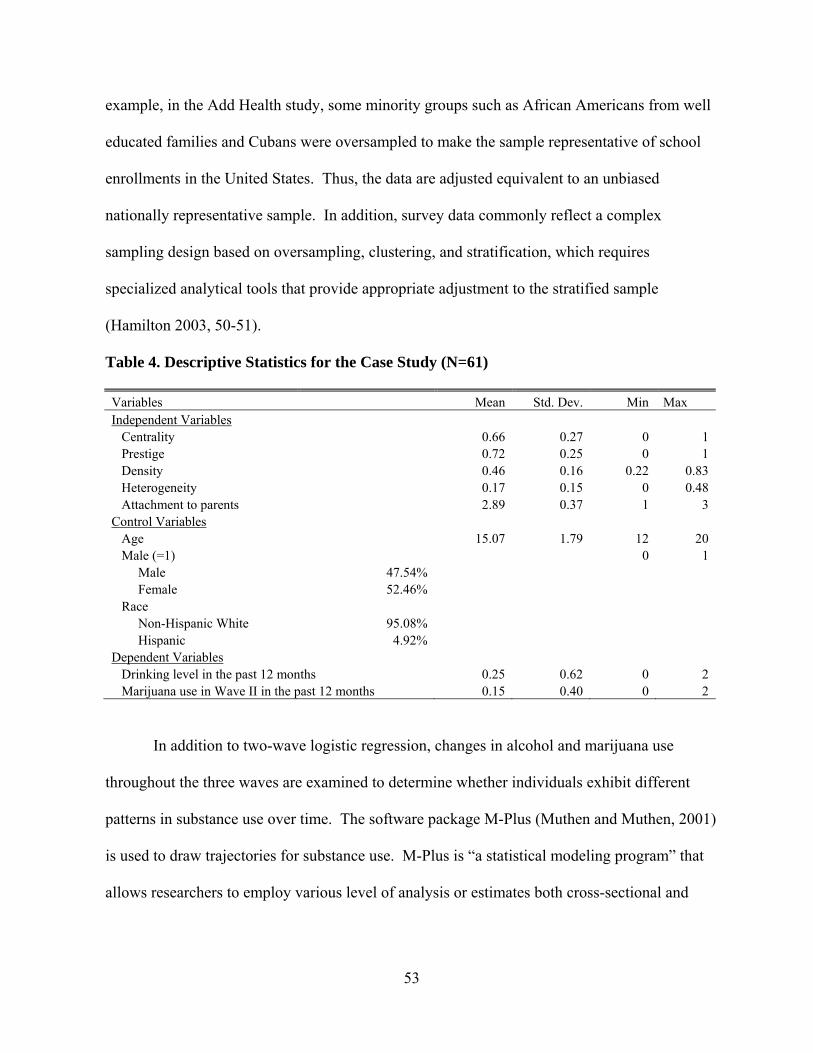
53
example, in the Add Health study, some minority groups such as African Americans from well
educated families and Cubans were oversampled to make the sample representative of school
enrollments in the United States. Thus, the data are adjusted equivalent to an unbiased
nationally representative sample. In addition, survey data commonly reflect a complex
sampling design based on oversampling, clustering, and stratification, which requires
specialized analytical tools that provide appropriate adjustment to the stratified sample
(Hamilton 2003, 50-51).
Table 4. Descriptive Statistics for the Case Study (N=61)
Variables Mean Std. Dev. Min Max Independent Variables Centrality 0.66 0.27 0 1 Prestige 0.72 0.25 0 1 Density 0.46 0.16 0.22 0.83 Heterogeneity 0.17 0.15 0 0.48 Attachment to parents 2.89 0.37 1 3 Control Variables Age 15.07 1.79 12 20 Male (=1) 0 1 Male 47.54% Female 52.46% Race Non-Hispanic White 95.08% Hispanic 4.92% Dependent Variables Drinking level in the past 12 months 0.25 0.62 0 2 Marijuana use in Wave II in the past 12 months 0.15 0.40 0 2
In addition to two-wave logistic regression, changes in alcohol and marijuana use
throughout the three waves are examined to determine whether individuals exhibit different
patterns in substance use over time. The software package M-Plus (Muthen and Muthen, 2001)
is used to draw trajectories for substance use. M-Plus is “a statistical modeling program” that
allows researchers to employ various level of analysis or estimates both cross-sectional and
54
longitudinal data (see Muthen and Muthen, M-Plus homepage, retrieved on February 15, 2010:
http://www.statmodel.com/features.shtml).
In terms of changes in the level of substance use, a Latent Growth Mixture Model
(LGMM) is used to draw meaningful trajectories of substance use from late teens to mid-
twenties among the entire sample. Selecting models that exhibit significant difference in
behavioral patterns is sought within a Bayesian context (Bayes 1763).15 Here Schwartz’s
Bayesian information Criterion (BIC)16 is used because it maximizes the function of models to
choose from others that include different numbers of models.
A conventional growth model estimates a developmental trajectory for the population
based on individual differences. In contrast, the LGMM (see Wiesner and Windle 2004: 435)
assumes that “the population is composed of a mixture of distinct subgroups, each defined by a
prototypical growth curve.” Since each individual is supposed to have a different level of
substance involvement and trajectory pattern, I attempt to identify a number of distinct
pathways in substance use based on the characteristics of one’s friendship network. The
LGMM is better suited to the task than Hierarchical Linear Model (HLM). Although HLM
captures within- and between-person differences such as gender and race (Horney et al. 1995)
LGMM identifies the full variation of the data, that is, multiple unobserved trajectories.
Because individual differences beyond the traditional demographic differences listed above are
of interest here, the LGMM is most appropriate.
15 Responding to Schwartz’s criticism that “the maximum likelihood (ML) principle invariably leads to choosing the highest possible dimension (1978, 461)” to fit observations, Akaike (1974) expanded the ML principle to choose a best-fit model among different parameters by running ML separately for different models. However, Akaike’s expansion, which is referred to as the Akaike Information Criterion (AIC), has been criticized for its inconsistency (see Kashyap, 1980). 16 BIC=-2logL+r ln n where L=the maximized value of the likelihood function for an estimated model: r=the number of free parameters to be estimated; and n=the number of observations.

55
For the case study, UCINET (by Roberta Chase and Steve Borgatti) is used to create a
sociomatrix and sociogram to describe interpersonal and structural connections within a given
group. UCINET, which allows us to grasp the individuals’ positions within their networks, is
an excellent tool to provide detailed network connections graphically. Further, according to
Scott (1991: 117), it also offers us an instrument to divide the sample into subgroups such as
cliques that consist of a subset of nodes of three of more in which “every possible pair of nodes
is directly connected by a line and the clique is not contained in any other clique.”

56
CHAPTER FIVE
QUANTITATIVE STUDY: FINDINGS AND DISCUSSION
Introduction
In this chapter I examine the relationship between network characteristics and substance
use. The focus of the regression analyses relating to Hypothesis 1 is on how structural
proximity to one’s friends at Wave I affects the use of alcohol and marijuana at Wave II. This
hypothesis is tested using different models to determine the effects of the network variables
Centrality, Prestige, Density, and Heterogeneity. I also examine whether the effects of the
network variables on substance use increase when the level of attachment to parents is held
constant.
Although a positive relationship between early and later substance use has been well-
documented by criminologists (for discussions, see Cairns and Cairns 1994; Barnes et al. 1992),
the potential long-term effects of early friendships on later substance use has not been
examined systematically. The analyses testing Hypothesis 2 examine the relationship between
the respondents’ positions in early friendship networks and substance use at Wave III as
respondents move into adulthood. Finally, I examine Hypothesis 3, which deals with long-term
behavioral trajectories for alcohol and marijuana use.
Hypothesis 1
Four initial models are used to address Hypothesis 1, which states that the greater the
Centrality, Prestige, and Heterogeneity of an individual’s location in a social network, the
greater the likelihood the individual will engage in substance use; and, the greater the Density
57
of an individual’s social network, the less likely it is that the individual will engage in
substance use.
Model 1 addresses the role of Centrality, which refers to an actor’s activeness in
nominating others as friends. Greater Centrality is expected to be associated with higher levels
of substance use because these individuals are assumed to have greater opportunities to engage
in substance use. Model 2 examines Prestige, which refers to the popularity of an actor. If we
assume that alcohol or drug use is acceptable behavior among adolescents, then the more often
an actor is nominated as a friend by others, or is popular in one’s peer group, the more likely it
is that the actor will be a substance user. Model 3 addresses the Density or cohesiveness of an
actor’s friendship groups. If we assume that cohesiveness in groups reflects strong attachment
to conventional peers, then youth in less cohesive groups should have greater freedom to
engage in prohibited behaviors and therefore have higher levels of substance use. Model 4
examines the effect of the degree of racial/ethnic Heterogeneity within groups. Here it is
assumed that heterogeneous groups will be characterized by a diversity of values or attitudes
toward substance use. As such, these groups are less likely than homogeneous groups to be
cohesive and less consistent in the enforcement of conventional controls. Actors in such
groups are expected to have higher levels of substance use.
Finally, Models 5 through 7 explore whether the effects of the network variables are
increased when attachment to parents is controlled. Because attachment to parents is assumed
to be a source of conventional social control, it is expected that strong attachment to parents
will serve as a constraining factor with respect to substance use. If true, and assuming that
everyone equally attached to their parents, the effects of the network variables should be
strengthened.
58
As the intercorrelations among the variables reported in Table 5 reveal, all of the
independent variables are correlated with both alcohol and marijuana use. In addition, age is
positively correlated with substance use while sex is positively correlated with these behaviors
indicating that substance users are most likely to be older and male. It should be noted that
although the correlation coefficients are statistically significant most are small. This is no
doubt due in part to the skewed distributions of the substance use measures, which is typical in
this type of study. Nevertheless, these findings suggest some initial support for Hypothesis 1.
For example, Prestige is positively associated with both alcohol and marijuana use and Density
is negatively associated with both substances. On the other hand, the correlation between
Centrality and substance use is just the opposite from the hypothesized direction, and
Heterogeneity varies by substance type. A somewhat different picture emerges when I turn to
the regression analysis.
Alcohol Use
The results for Model 1 are reported in Table 6 and indicate that Centrality does not
have the expected positive effect on alcohol use. Greater Centrality of an actor in a group, at
least as measured here, has no apparent effect on alcohol use.
Similarly, Model 2 reveals that like Centrality, Prestige has no effect on alcohol use.
Prestige, or popularity, was expected to be associated with a greater likelihood of underage
drinking. It may be that because alcohol is an easily accessible substance, one’s position in a
network makes little difference. An alternative explanation is that popular individuals are more
likely to be law-abiding and thus nominated by non-delinquent friends who represent the
majority of respondents. Some suggestive evidence of this can be seen given the findings
regarding Density.
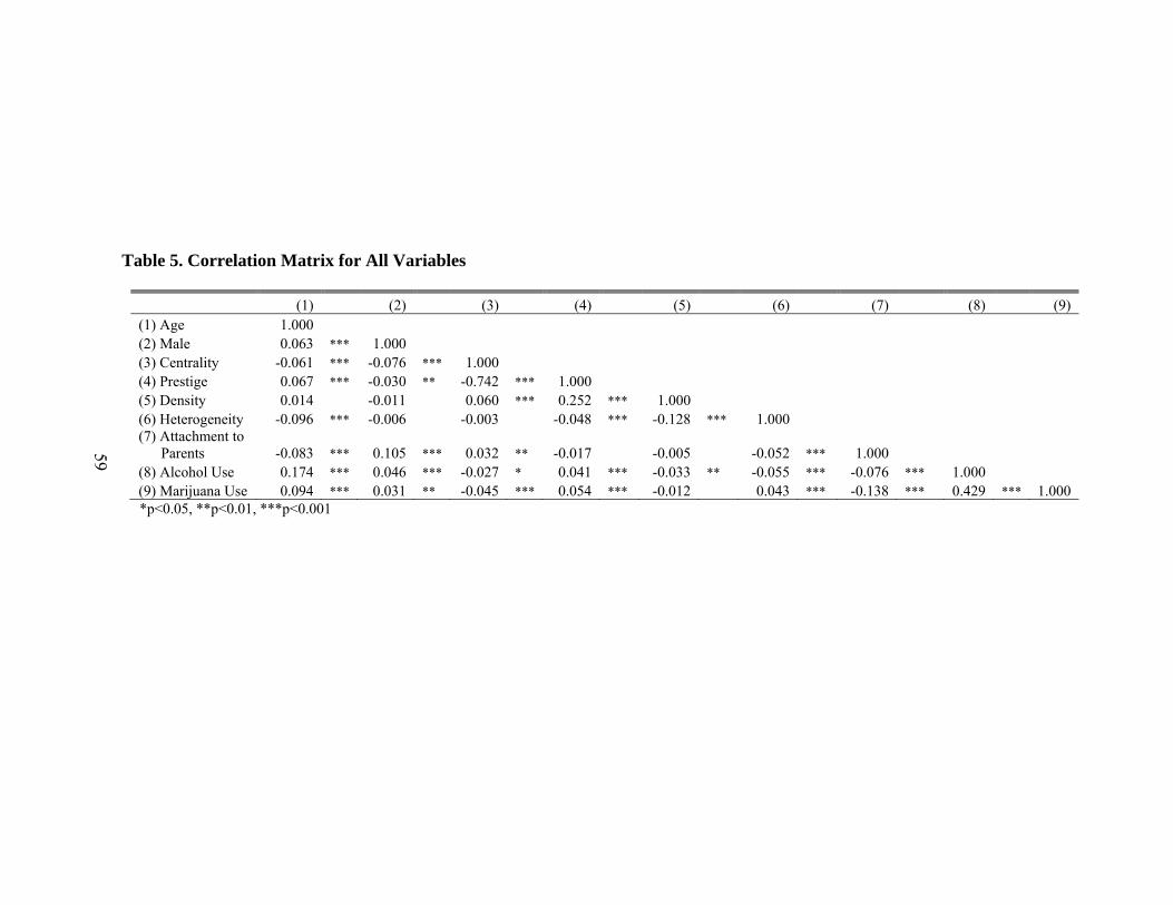
59
Table 5. Correlation Matrix for All Variables
(1) (2) (3) (4) (5) (6) (7) (8) (9) (1) Age 1.000 (2) Male 0.063 *** 1.000 (3) Centrality -0.061 *** -0.076 *** 1.000 (4) Prestige 0.067 *** -0.030 ** -0.742 *** 1.000 (5) Density 0.014 -0.011 0.060 *** 0.252 *** 1.000 (6) Heterogeneity -0.096 *** -0.006 -0.003 -0.048 *** -0.128 *** 1.000 (7) Attachment to Parents -0.083 *** 0.105 *** 0.032 ** -0.017 -0.005 -0.052 *** 1.000 (8) Alcohol Use 0.174 *** 0.046 *** -0.027 * 0.041 *** -0.033 ** -0.055 *** -0.076 *** 1.000 (9) Marijuana Use 0.094 *** 0.031 ** -0.045 *** 0.054 *** -0.012 0.043 *** -0.138 *** 0.429 *** 1.000
*p<0.05, **p<0.01, ***p<0.001

60
Table 6. Network Characteristics on Alcohol Use at Wave II (N=7,106)
Variable Model 1 Model 2 Model 3 Model 4 Age 0.26 *** 0.26 *** 0.27 *** 0.26 ***
(0.02) (0.02) (0.02) (0.02)
Male -0.09 -0.07 -0.08 -0.08
(0.07) (0.07) (0.07) (0.07)
African American -0.83 *** -0.82 *** -0.83 *** -0.81 ***
(0.12) (0.12) (0.13) (0.12)
Hispanic -0.09 -0.08 -0.07 -0.06
(0.11) (0.11) (0.12) (0.12)
Asian -0.82 *** -0.83 *** -0.78 *** -0.81 ***
(0.19) (0.19) (0.19) (0.19)
Native American -0.28 -0.27 -0.29 0.27
(0.28) (0.28) (0.28) (0.28)
Centrality -0.16
(0.11)
Prestige 0.25
(0.13)
Density -0.77 *
(0.33)
Heterogeneity -0.09
(0.22)
F 0.00 *** 0.00 *** 0.00 *** 0.00 *** *p<0.05, **p<0.01, ***p<0.001 Race/ethnicity is in reference to Whites. Values in parentheses are linearized standard errors.
Consistent with my hypothesis, Model 3 shows that group Density or cohesiveness has a
significant negative effect on alcohol use. Individuals who belong to cohesive groups are less
likely to drink. Cohesive groups appear to serve as a source of conventional social control and
thus constrain rather than facilitate adolescent drinking. This is consistent with the findings
reported by Burkett (1977b) that isolation from conventional social activities may lead to heavy
involvement of alcohol and drug use. The finding is also consistent with Haynie’s (2001) study,
which suggests that Density is negatively associated with delinquency involvement when all
other variables are controlled.
Groups characterized by racial/ethnic heterogeneity were hypothesized to be less
constraining with regard to adolescent drinking than more homogeneous groups. That is,

61
racial/ethnic heterogeneous groups are expected to lack solidarity with respect to the
enforcement of conventional social controls relating to substance use. In the absence of such
controls substance use is more likely to occur. As noted in Table 5, Heterogeneity is negatively
correlated with Density, which suggests that heterogeneous groups are less cohesive. However,
the findings do not support the hypothesis that Heterogeneity increases the likelihood of
drinking. Model 4 shows that Heterogeneity has no apparent effect on underage drinking.
Interestingly, when the network characteristics are examined together (see Model 5 in
Table 7) still another picture emerges. In addition to Density, Prestige now shows a significant
effect on drinking. It appears that popular individuals are more likely to engage in underage
drinking, but that those in cohesive groups are less likely to drink. In other words, someone
who is popular, but belongs to a loosely organized group is most likely to engage in underage
drinking. Furthermore, although individuals are recognized and nominated by others, they
rarely reciprocate by nominating others as friends. This may contribute to the appearance of a
lack of cohesiveness in the groups to which they belong. This appears to be similar to what
Yablonsky (1959) refers to as a “near-group,” which is loosely organized around a sometimes
charismatic “leader.”
Consistent with past research, these findings show that youth who drink tend to be
somewhat older than those who do not. However, in these models differences by sex appear to
be negated. This discrepancy between the correlations and the regression analysis is explained
by the effects of other independent variables.
Among the network variables, attachment to parents is positively correlated with
Centrality and negatively correlated with Heterogeneity (see Table 5). Social control theory
suggests that youth who are strongly attached to their parents are unlikely to choose friends

62
who are substance users, whereas those who do not have such ties are more likely to do so.
The network variables, which are generally consistent with social learning theory, suggest that
those who are involved with substance users are likely to be subject to socialization to within
friendship group expectations. Therefore, it is necessary to examine how the effects of the
network variables change when attachment to parents is controlled.
Table 7. The Effects of the Network Variables on Alcohol Use When Attachment to Parents is Held Constant (N=7,040)
Variable Model 5 Model 6 Model 7 Age 0.26 *** 0.25 *** 0.24 ***
(0.02) (0.02) (0.02)
Sex -0.05 -0.04 0.00
(0.07) (0.07) (0.07)
African American -0.78 *** -0.91 *** -0.88 ***
(0.12) (0.12) (0.12)
Hispanic 0.00 -0.10 -0.01
(0.12) (0.11) (0.11)
Asian -0.70 *** -0.81 *** -0.70 ***
(0.19) (0.19) (0.19)
Native American -0.27 -0.31 -0.31
(0.28) (0.27) (0.28)
Centrality 0.36 0.39 *
(0.18) (0.19)
Prestige 0.65 ** 0.69 ***
(0.21) (0.21)
Density -1.16 ** -1.22 **
(0.37) (0.38)
Heterogeneity -0.22 -0.27
(0.23) (0.23)
Attachment to Parents -0.32 *** -0.34 ***
(0.06) (0.06)
F 0.00 *** 0.00 *** 0.00 *** * p<0.05, **p<0.01, ***p<0.001 Race/ethnicity is in reference to Whites. Values in parentheses are linearized standard errors.
Attachment to parents has, as expected, a strong negative effect on alcohol use (see
Model 6 in Table 7). As control theory suggests, attachment to parents serves as a constraining
factor. When the effect of attachment to parents is included in Model 7 (Table 7), Centrality
shows a significant positive effect on alcohol use. In addition, the positive effect of Prestige

63
and the negative effect of Density are stronger. Clearly attachment to parents has a significant
impact on adolescent alcohol use, but when attachment to parents is controlled the effects of the
network variables on alcohol use are stronger. For example, the significance level of Density
increased, and Centrality became significant. Although the coefficient of attachment to parents
is marginally increased by controlling for the network variables, the change is not statistically
significant.17 Overall, Hypothesis 1 for alcohol use is partially supported.
Although not addressed to this point, it is apparent from the models examined that with
the possible exception of Native Americans, there are significant differences in levels of
alcohol use by race/ethnic groups. For example, the mean drinking level of Whites is
significantly greater than for African Americans and Asians (Table 8). The findings also reveal
that as a group, Hispanic youth drink significantly more than either African American or Asian
youth. These differences are borne out when I examine racial/ethnic differences in alcohol use
using One-Way Analysis of Variance or ANOVA. Because there are five racial/ethnic
categories in the sample, the Scheffé multiple-comparison test is used to determine the
differences between each pair of means (Hamilton, 1998: 117). As noted, the results reveal
significant racial/ethnic differences in the levels of alcohol use. To understand to role of
racial/ethnic differences, interaction terms are examined for each of the previous models (see
Table 9, Models 1a-4a).
When the interaction terms are examined, Centrality becomes significant and serves as
constraining factor for some youth. For example, Centrality has a significant positive effect on
drinking among African Americans. Thus, the initial hypothesis regarding Centrality is
supported, but only among African Americans. For these youth, the general effect of
17 Although it is not within the scope of this study, when the effects of the network variables are examined by the levels of attachment to parents, the results are inconsistent or non-significant.
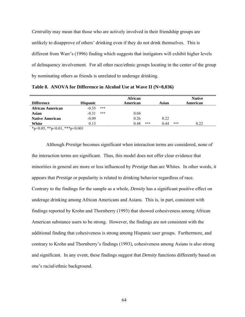
64
Centrality may mean that those who are actively involved in their friendship groups are
unlikely to disapprove of others’ drinking even if they do not drink themselves. This is
different from Warr’s (1996) finding which suggests that instigators will exhibit higher levels
of delinquency involvement. For all other race/ethnic groups locating in the center of the group
by nominating others as friends is unrelated to underage drinking.
Table 8. ANOVA for Difference in Alcohol Use at Wave II (N=8,036)
Difference Hispanic African
American Asian Native
American African American -0.35 *** Asian -0.31 *** 0.04 Native American -0.09 0.26 0.22 White 0.13 0.48 *** 0.44 *** 0.22 *p<0.05, **p<0.01, ***p<0.001
Although Prestige becomes significant when interaction terms are considered, none of
the interaction terms are significant. Thus, this model does not offer clear evidence that
minorities in general are more or less influenced by Prestige than are Whites. In other words, it
appears that Prestige or popularity is related to drinking behavior regardless of race.
Contrary to the findings for the sample as a whole, Density has a significant positive effect on
underage drinking among African Americans and Asians. This is, in part, consistent with
findings reported by Krohn and Thornberry (1993) that showed cohesiveness among African
American substance users to be strong. However, the findings are not consistent with the
additional finding that cohesiveness is strong among Hispanic user groups. Furthermore, and
contrary to Krohn and Thornberry’s findings (1993), cohesiveness among Asians is also strong
and significant. In any event, these findings suggest that Density functions differently based on
one’s racial/ethnic background.

65
Table 9. Interaction Effects with Network Characteristics on Alcohol Use at Wave II (N=7,040)
Variable
Centrality
Prestige
Density
Heterogeneity
Model 1-a Model 2-a Model 3-a Model 4-a Age 0.27 *** 0.26 *** 0.27 *** 0.26 ***
(0.02) (0.02) (0.02) (0.02) Male -0.09 -0.07 -0.08 -0.08
(0.07) (0.07) (0.07) (0.07)
African American -1.30 *** -0.47 -1.34 *** -0.78 ***
(0.24) (0.25) (0.30) (0.18)
Hispanic -0.25 0.19 -0.37 0.16
(0.20) (0.26) (0.26) (0.25)
Asian -1.35 ** -0.10 -1.52 *** -1.18 ***
(0.42) (0.47) (0.36) (0.21)
Native American -0.60 -0.03 -0.78 -1.37 *
(0.59) (0.75) (0.54) (0.63)
Network variable -0.35 * 0.41 * -1.26 ** -0.19
(0.15) (0.17) (0.41) (0.26) Network variable x African American 0.81 * -0.56 1.84 * -0.09
(0.33) (0.34) (0.85) (0.42) Network variable x Hispanic 0.26 -0.28 1.02 -0.41
(0.33) (0.35) (0.69) (0.57) Network variable x Asian 0.86 -1.13 2.24 * 1.02
(0.51) (0.70) (0.78) (0.68) Network variable x Native American 0.52 -0.39 1.82 3.71
(0.98) (1.12) (2.01) (1.93)
F 0.00 *** 0.00 *** 0.00 *** 0.00 *** *p<0.05, **p<0.01, ***p<0.001 Race/ethnicity is in reference to Whites. Values in parentheses are linearized standard errors.
When the variable Heterogeneity is examined, I find virtually no interaction effects on
drinking. However, drinking among Native Americans does appear to be significantly different
from Whites. When all other variables including the interaction terms are controlled (see
Model 4-a) the drinking level among Native Americans is significantly lower than Whites.
This is, perhaps somewhat surprising given the fact that according to the 2008 population
statistics (see U.S. Census Bureau 2000: Table 3), Native Americans comprise only 1.01
percent of total population in the United States. However, given the even smaller number who
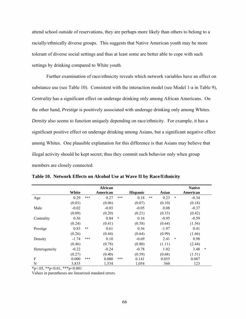
66
attend school outside of reservations, they are perhaps more likely than others to belong to a
racially/ethnically diverse groups. This suggests that Native American youth may be more
tolerant of diverse social settings and thus at least some are better able to cope with such
settings by drinking compared to White youth.
Further examination of race/ethnicity reveals which network variables have an effect on
substance use (see Table 10). Consistent with the interaction model (see Model 1-a in Table 9),
Centrality has a significant effect on underage drinking only among African Americans. On
the other hand, Prestige is positively associated with underage drinking only among Whites.
Density also seems to function uniquely depending on race/ethnicity. For example, it has a
significant positive effect on underage drinking among Asians, but a significant negative effect
among Whites. One plausible explanation for this difference is that Asians may believe that
illegal activity should be kept secret; thus they commit such behavior only when group
members are closely connected.
Table 10. Network Effects on Alcohol Use at Wave II by Race/Ethnicity
White African
American Hispanic Asian Native
American Age 0.29 *** 0.27 *** 0.18 ** 0.23 * -0.34
(0.03) (0.06) (0.07) (0.10) (0.18)
Male -0.02 -0.03 -0.05 0.08 -0.37
(0.09) (0.20) (0.21) (0.33) (0.42)
Centrality 0.36 0.84 * 0.16 -0.95 -0.59
(0.24) (0.41) (0.58) (0.64) (1.56)
Prestige 0.83 ** 0.61 0.36 -1.97 0.41
(0.26) (0.44) (0.64) (0.99) (1.66)
Density -1.74 *** 0.10 -0.69 2.41 * 0.98
(0.46) (0.78) (0.80) (1.11) (2.44)
Heterogeneity -0.22 -0.24 -0.78 1.02 3.48 *
(0.27) (0.40) (0.59) (0.68) (1.51) F 0.000 *** 0.000 *** 0.141 0.055 0.087 N 3,835 1,534 1,054 560 123
*p<.05, **p<0.01, ***p<0.001 Values in parentheses are linearized standard errors.
67
Finally, when I examine alcohol use within race/ethnicity, Heterogeneity has a
significant positive effect on underage drinking only among Native Americans. Furthermore,
when the social network variables are examined together, the effect of Heterogeneity continues
to show a significant positive association with underage drinking among Native Americans.
There are at least two plausible explanations for this finding. First, based on socialization
model, members of heterogeneous groups are more likely to be exposed to and possibly accept
different values and therefore behave accordingly. For Native Americans, Heterogeneity in
groups may create different opportunities to engage in alcohol use, which in turn, may increase
the likelihood of drinking when other social network factors are taken into account. Second, it
is also possible that Native Americans are likely to experience social isolation and when
possible, selectively choose other Native Americans as friends. However, failing that due to
the small number of choices, such negative experiences may result in more drinking as a means
of coping with social isolation and a lack of conventional social controls even though they may
still drink less than Whites.
As noted earlier, when drinking by Native Americans is compared to Whites and
Heterogeneity is examined alone, Native Americans drink less than Whites (Table 9).
However, when Heterogeneity is examined within race/ethnicity it appears to have no
significant effect among White youth (Table 10). This may be due to the fact that given their
large numbers, White youth are less likely to be in racially/ethnically diverse friendship groups.
My interpretation with the findings in these two Tables is that Heterogeneity in general does
not have an effect on underage drinking among White youth, but when they happen to be in a
racially/ethnically diverse group Whites are more likely to drink. On the other hand, because
Native Americans are more likely to be in racially/ethnically diverse groups when attending
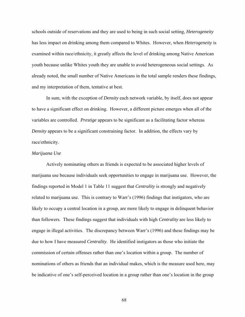
68
schools outside of reservations and they are used to being in such social setting, Heterogeneity
has less impact on drinking among them compared to Whites. However, when Heterogeneity is
examined within race/ethnicity, it greatly affects the level of drinking among Native American
youth because unlike Whites youth they are unable to avoid heterogeneous social settings. As
already noted, the small number of Native Americans in the total sample renders these findings,
and my interpretation of them, tentative at best.
In sum, with the exception of Density each network variable, by itself, does not appear
to have a significant effect on drinking. However, a different picture emerges when all of the
variables are controlled. Prestige appears to be significant as a facilitating factor whereas
Density appears to be a significant constraining factor. In addition, the effects vary by
race/ethnicity.
Marijuana Use
Actively nominating others as friends is expected to be associated higher levels of
marijuana use because individuals seek opportunities to engage in marijuana use. However, the
findings reported in Model 1 in Table 11 suggest that Centrality is strongly and negatively
related to marijuana use. This is contrary to Warr’s (1996) findings that instigators, who are
likely to occupy a central location in a group, are more likely to engage in delinquent behavior
than followers. These findings suggest that individuals with high Centrality are less likely to
engage in illegal activities. The discrepancy between Warr’s (1996) and these findings may be
due to how I have measured Centrality. He identified instigators as those who initiate the
commission of certain offenses rather than one’s location within a group. The number of
nominations of others as friends that an individual makes, which is the measure used here, may
be indicative of one’s self-perceived location in a group rather than one’s location in the group

69
as defined by others. Those that an individual selects as friends may not provide greater
opportunities to engage in marijuana use.
Table 11. Network Characteristics on Marijuana Use at Wave II (N=6,943)
Variable Model 1 Model 2 Model 3 Model 4 Age 0.17 *** 0.17 *** 0.18 *** 0.20 ***
(0.03) (0.03) (0.03) (0.03) Male -0.08 -0.05 -0.05 -0.05 (0.11) (0.10) (0.11) (0.11) African American -0.14 -0.10 -0.11 -0.17 (0.14) (0.14) (0.14) (0.14) Hispanic 0.13 0.16 0.18 -0.03 (0.14) (0.14) (0.14) (0.15) Asian -0.77 ** -0.77 ** -0.74 ** -0.91 ***
(0.25) (0.25) (0.25) (0.25)
Native American 0.70 ** 0.72 ** 0.71 ** 0.68 *
(0.26) (0.25) (0.26) (0.26)
Centrality -0.45 ***
(0.13)
Prestige 0.51 ***
(0.12) Density -0.50 (0.30) Heterogeneity 0.75 ***
(0.22)
F 0.00 *** 0.00 *** 0.00 *** 0.00 *** *p<0.05, **p<0.01, ***p<0.001 Race/ethnicity is in reference to Whites. Values in parentheses are linearized standard errors.
As expected, Prestige does have a significant positive effect on marijuana use (Model
2). One’s popularity in a friendship network is perhaps more likely to play a crucial role for
marijuana use because compared to alcohol, marijuana is not as readily accessible. Therefore,
juveniles who are the center of attention may have greater opportunities to experience
marijuana with their friends. It may also be the case that those who already use marijuana are
perceived as “cool” and are selected as friends for this reason.
Unlike alcohol use, Density does not have a significant effect on marijuana use (Table
11, Model 3). Within group cohesiveness is apparently unrelated to the use of marijuana.

70
Although network connections may be necessary for an initial experience, once involved in
marijuana use, adolescents do not appear to be bound to a cohesive group.
Finally, the findings regarding Heterogeneity are consistent with my expectation that
members of heterogeneous groups are more likely to use marijuana. This is indicated by the
significant positive effect on marijuana use (see Model 4 in Table 11). Racial/ethnic
heterogeneity in friendship groups may weaken the level of cohesiveness in group, which in
turn, facilitates marijuana use due to the lack of conventional control from others (r between
Density and Heterogeneity=-0.128). Racial/ethnic heterogeneity may also be indicative of
diverse and possibly competing value/belief systems within such groups. If true, this finding is
consistent with the notion that adolescents in heterogeneous groups are more likely to be
exposed to values supportive of marijuana use.
The above makes a little more sense when I examine what happens when all of the
independent variables are included. When all the network variables are included the effect of
Centrality is canceled out. Consistent with Models 1 through 4, Prestige and Heterogeneity
have significant positive effects on marijuana use. The entire model is consistent with the
notion that friendship networks are necessary for individuals to develop attitudes favorable to
marijuana use and to engage in the behavior. For example, in heterogeneous groups where
diverse values or definitions favorable toward marijuana use are potentially more likely,
individuals are also more likely to be users. Given exposure to normative values different from
their own, marijuana use may very well be based on newly developed attitudes as a product of
socialization. At the same time, it may be that some may choose to belong to heterogeneous
groups that appear to have normative values and standards similar to their own. Furthermore,

71
popular individuals are more likely to engage in marijuana use or alternatively, marijuana users
tend to be popular among non-users who aspire to be like them.
As was true for alcohol use, Model 6 in Table 12 shows that attachment to parents has a
significant negative effect on marijuana use. Consistent with alcohol use, when all independent
variables are incorporated in Model 7, Centrality remains non-significant. However, Density is
significantly and negatively related to marijuana use. Prestige has a significant positive effect
on marijuana use and its effect is stronger. The differences from the findings for alcohol use
are that Heterogeneity has a significant positive effect on marijuana use while Centrality has no
effect. This seems to be consistent with Orcutt’s study (1978) of alcohol and marijuana use in
which he found that marijuana use is more acceptable than alcohol when the subject’s
motivation is “personal” rather than “social.” That is, smoking marijuana is acceptable in a
small though not necessarily cohesive group of friends as a means of coping with the stresses of
school or not “fitting in” compared to drinking alcohol to withdraw from a boring party.
The entire model shows that attachment to parents still has a significant negative effect
on marijuana use, but the effect is virtually the same when the network variables are included.
That is, among adolescents, attachment to parents is not affected by the network variables
whereas the network variables are influenced when attachment to parents is controlled. Among
adolescents, friendship networks are undoubtedly a major socialization agency, and when the
impact of parents is controlled youth are more likely to be affected by the friendship network
position with regard to marijuana use.
As with alcohol use, age is clearly related to individual use of marijuana, that is, youth
who engage in marijuana use tend to be older than non-users. When age is controlled, all of the
network variables except for Centrality show a significant influence on marijuana use.
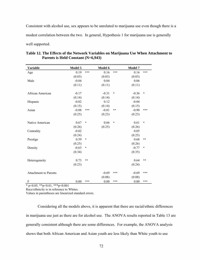
72
Consistent with alcohol use, sex appears to be unrelated to marijuana use even though there is a
modest correlation between the two. In general, Hypothesis 1 for marijuana use is generally
well supported.
Table 12. The Effects of the Network Variables on Marijuana Use When Attachment to Parents is Held Constant (N=6,943)
Variable Model 5 Model 6 Model 7 Age 0.19 *** 0.16 *** 0.16 ***
(0.03) (0.03) (0.03)
Male -0.04 0.04 0.06
(0.11) (0.11) (0.11)
African American -0.17 -0.31 * -0.36 *
(0.14) (0.14) (0.14)
Hispanic -0.02 0.12 -0.04
(0.15) (0.14) (0.15)
Asian -0.88 *** -0.81 ** -0.90 ***
(0.25) (0.23) (0.23)
Native American 0.67 * 0.66 * 0.61 *
(0.26) (0.25) (0.26)
Centrality -0.02 0.05
(0.24) (0.25)
Prestige 0.59 * 0.68 **
(0.25) (0.26)
Density -0.63 * -0.77 *
(0.34) (0.35)
Heterogeneity 0.73 ** 0.64 **
(0.23) (0.24)
Attachment to Parents -0.69 *** -0.69 ***
(0.08) (0.08)
F 0.00 *** 0.00 *** 0.00 *** * p<0.05, **p<0.01, ***p<0.001 Race/ethnicity is in reference to Whites. Values in parentheses are linearized standard errors.
Considering all the models above, it is apparent that there are racial/ethnic differences
in marijuana use just as there are for alcohol use. The ANOVA results reported in Table 13 are
generally consistent although there are some differences. For example, the ANOVA analysis
shows that both African American and Asian youth are less likely than White youth to use

73
marijuana. The fact that there are differences between groups suggests that the interaction
effects of the network variables with race/ethnicity need to be examined.
Table 13. ANOVA for Difference in Marijuana Use at Wave II (N=7,942)
Difference
Hispanic African
American Asian Native
American African American -0.08 * Asian -0.13 ** -0.05 Native American 0.10 0.18 * 0.23 ** White -0.01 0.07 ** 0.12 *** -0.11
*p<0.05, **p<0.01, ***p<0.001
When the interaction terms are included in each model, all of the network variables are
significantly related to marijuana use though the direction varies. Centrality continues to have
a significant negative effect on marijuana use (Table 14, Model 1-a). Unlike alcohol use,
Centrality does not have any effect for marijuana use among African Americans. On the other
hand, Prestige has a significant positive effect on marijuana use regardless of race/ethnicity
(Model 2-a) and popular individuals are more likely to use marijuana.
In general, Density (see Model 3-a) appears to be a constraining factor for the sample as
a whole. Since the sample is predominantly White, the overall effect may be due to their large
numbers. However, whereas the general effect of Density is negative, it is positively associated
with marijuana use among African American and Hispanic youth. This is consistent with the
findings reported by Krohn and Thornberry (1993) that both African American and Hispanic
alcohol and marijuana users are more intimately related to one another than are non-users. For
these racial/ethnic groups, adolescents that use marijuana are likely to be members of relatively
cohesive groups. Why and how these differences occur is beyond the scope of this
investigation, but a plausible explanation is that certain racial/ethnic groups are more likely to
hide their illegal behavior from those outside their group and to demand loyalty to the group.

74
Table 14. Interaction Effects with Network Characteristics on Marijuana Use at Wave II (N=6,943)
Variable Centrality
Prestige
Density
Heterogeneity
Model 1-a Model 2-a Model 3-a Model 4-a Age 0.17 *** 0.17 *** 0.18 *** 0.20 ***
(0.03) (0.03) (0.03) (0.03)
Male -0.08 -0.05 -0.05 -0.05
(0.11) (0.11) (0.11) (0.11)
African American -0.40 0.04 -0.76 *** -0.05
(0.24) (0.25) (0.21) (0.23)
Hispanic -0.05 0.30 -0.27 0.57
(0.26) (0.30) (0.23) (0.38)
Asian -0.81 -0.58 -0.69 -1.09
(0.41) (0.54) (0.61) (0.55)
Native American -0.06 1.15 -0.29 0.98 * (0.53) (0.61) (0.56) (0.46)
Network variable -0.61 *** 0.60 *** -1.10 ** 0.96 ***
(0.17) (0.16) (0.38) (0.26) Network variable x African American 0.45 -0.22 2.30 *** -0.42
(0.31) (0.37) (0.63) (0.55) Network variable x Hispanic 0.31 -0.23 1.50 * -1.36
(0.37) (0.41) (0.63) (0.73) Network variable x Asian -0.06 -0.30 -0.04 0.31
(0.57) (0.81) (2.01) (1.21) Network variable x Native American 1.25 -0.70 1.52 -1.11
(0.81) (0.91) (1.99) (1.39)
F 0.00 *** 0.00 *** 0.00 *** 0.00 *** *p<0.05, **p<0.01, ***p<0.001 Race/ethnicity is in reference to Whites. Values in parentheses are linearized standard errors.
Whereas Density has a negative effect on marijuana use, Heterogeneity has a significant
positive effect on marijuana use regardless of racial/ethnic group (Model 4-a). That is, an actor
in a heterogeneous group is more likely to use marijuana due at least in part to the lack of
cohesiveness characteristic of such groups. In addition, due to the different cultural
backgrounds of the group members, different value systems regarding certain behaviors are
perhaps more likely to co-exist in racially/ethnically heterogeneous groups. In such settings,
we can assume that individuals are more likely to accept rather than reject different values.
75
This appears inconsistent with the earlier findings, which suggested that African American and
Hispanic youth are more likely to engage in marijuana use in cohesive groups.
When interaction effects are considered, the network variables appear to have stronger
effects on marijuana use than was the case for alcohol use. The major difference between
alcohol and marijuana use is that only Heterogeneity has a significant positive effect on
marijuana use regardless of race/ethnicity. The reason for this difference is beyond the scope
of this study, but we can assume that because alcohol is a legal substance and underage
drinking is a status offense, competing normative values related to alcohol use are less likely to
exist.
Although we know how network variables function when the interaction terms are
embedded in these models, the independent effects of the network variables across racial/ethnic
groups are not entirely clear. For example, African American and Hispanic youth engage in
marijuana use in cohesive groups while the sample as a whole suggests that Heterogeneity
increases the likelihood for marijuana use. Thus, the effects of network variables by
race/ethnicity need to be examined more closely (see Table 15).
Among Whites, Prestige and Heterogeneity have significant positive effects on
marijuana use whereas Density has a significant negative effect. As already noted, Whites
typically belong to homogeneous groups in terms of race/ethnicity. Once the level of
Heterogeneity is controlled, they are likely to be susceptible to any diversity of values to which
they may be exposed and thus more likely to engage in marijuana use. None of the network
variables is significant among any of the other racial/ethnic groups.
In sum, Hypothesis 1 is relatively well supported for marijuana use. The findings
suggest that the network variables examined here have significant effects on substance use

76
although these effects vary by substance. That is, Centrality, Prestige, and Heterogeneity have
significant effects on marijuana use. Only Density has a significant effect on alcohol use. It is
also notable that for the sample as a whole the effects of Density and racial Heterogeneity are in
opposite directions. As the simple correlations suggest, these two variables are strongly and
negatively correlated. It appears then, that heterogeneous groups are less cohesive than are
homogeneous groups. Given within-group diversity, members are likely to be exposed to
different normative expectations or standards. At the same time, and perhaps due to competing
values, members are less likely to be constrained by conventional expectations. In the absence
of such controls, they are more likely to engage in marijuana use.
Table 15. Network Effects on Marijuana Use at Wave II by Race/Ethnicity
White African
American Hispanic Asian Native
American Age 0.24 *** 0.15 * 0.09 0.03 -0.46 *
(0.03) (0.06) (0.08) (0.14) (0.17) Male -0.12 0.69 *** -0.43 -0.18 -0.27 (0.14) (0.21) (0.22) (0.39) (0.44) Centrality -0.09 0.62 -0.29 -0.58 0.65 (0.32) (0.45) (0.51) (1.01) (1.02) Prestige 0.65 * 0.79 0.08 0.41 0.74 (0.32) (0.52) (0.65) (1.23) (1.42) Density -1.19 ** 0.93 0.18 -1.26 -0.74 (0.43) (0.54) (0.87) (2.41) (2.20) Heterogeneity 0.10 *** 0.53 -0.27 0.38 -0.37 (0.28) (0.45) (0.80) (1.50) (1.21) F 0.000 *** 0.001 *** 0.270 0.546 0.333 N 3,791 1,528 1,037 555 121
*p<.05, **p<0.01, ***p<0.001 Values in parentheses are linearized standard errors.
Finally, it should be noted again that among the four network variables, only Centrality
is based solely on an actor’s active nominations or wish to be a part of a group. In other words,
the negative effect of Centrality on marijuana use may reflect an actor’s one-way connection to
others. However, when dealing with an illegal substance, Prestige may be the most important

77
factor that affects marijuana use because recognition from others provides a wider range of
opportunities to engage in this behavior.
Hypothesis 2
Here I examine the extent to which one’s position in high school social networks
impacts the relationship between early and later substance use. Substance use in this case
includes alcohol and marijuana use, problem drinking, and the use of other illicit/unauthorized
drugs during the subjects’ mid-twenties as measured at Wave III.
Alcohol Use
It is common knowledge among criminologists and sociologists that underage drinking
is positively associated with later drinking behavior. The Add Health data are consistent with
this long-standing observation. The correlations between early and later alcohol use, and early
use and binge drinking and problems related to drinking are all significant (see Table 16).
Further, as noted in Model 1 in Table 17, the regression analysis reveals that early alcohol use
is positively associated with later alcohol use and related problems.
When Model 1 is expanded to include the network variables (see Model 2), the effect of
early drinking does not change. Furthermore, all of the network variables except Heterogeneity
are significant. Centrality and Prestige appear to predict later drinking whereas Density is
negatively associated with later drinking behavior. There is, however, some initial evidence
that there may be some differences by race/ethnicity. For example, by their mid- twenties, all
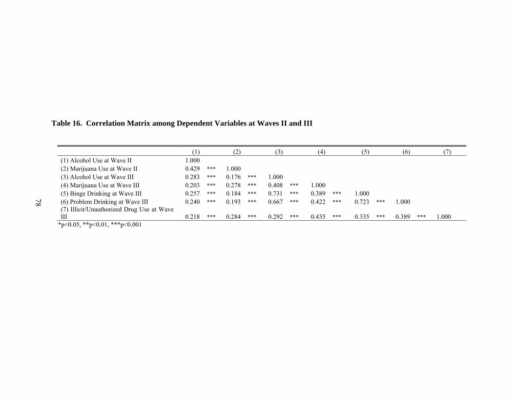
78
Table 16. Correlation Matrix among Dependent Variables at Waves II and III
(1) (2) (3) (4) (5) (6) (7) (1) Alcohol Use at Wave II 1.000 (2) Marijuana Use at Wave II 0.429 *** 1.000 (3) Alcohol Use at Wave III 0.283 *** 0.176 *** 1.000 (4) Marijuana Use at Wave III 0.203 *** 0.278 *** 0.408 *** 1.000 (5) Binge Drinking at Wave III 0.257 *** 0.184 *** 0.731 *** 0.389 *** 1.000 (6) Problem Drinking at Wave III 0.240 *** 0.193 *** 0.667 *** 0.422 *** 0.723 *** 1.000 (7) Illicit/Unauthorized Drug Use at Wave III 0.218 *** 0.284 *** 0.292 *** 0.435 *** 0.335 *** 0.389 *** 1.000
*p<0.05, **p<0.01, ***p<0.001
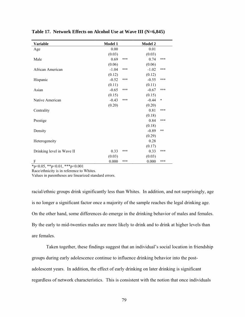
79
Table 17. Network Effects on Alcohol Use at Wave III (N=6,845)
Variable Model 1 Model 2 Age 0.00 0.01 (0.03) (0.03) Male 0.69 *** 0.74 ***
(0.06) (0.06)
African American -1.04 *** -1.02 ***
(0.12) (0.12)
Hispanic -0.52 *** -0.55 ***
(0.11) (0.11)
Asian -0.65 *** -0.67 ***
(0.15) (0.15)
Native American -0.43 *** -0.44 *
(0.20) (0.20)
Centrality 0.81 ***
(0.18)
Prestige 0.84 ***
(0.18)
Density -0.89 **
(0.29)
Heterogeneity 0.28
(0.17)
Drinking level in Wave II 0.33 *** 0.33 ***
(0.03) (0.03)
F 0.000 *** 0.000 *** *p<0.05, **p<0.01, ***p<0.001 Race/ethnicity is in reference to Whites. Values in parentheses are linearized standard errors.
racial/ethnic groups drink significantly less than Whites. In addition, and not surprisingly, age
is no longer a significant factor once a majority of the sample reaches the legal drinking age.
On the other hand, some differences do emerge in the drinking behavior of males and females.
By the early to mid-twenties males are more likely to drink and to drink at higher levels than
are females.
Taken together, these findings suggest that an individual’s social location in friendship
groups during early adolescence continue to influence drinking behavior into the post-
adolescent years. In addition, the effect of early drinking on later drinking is significant
regardless of network characteristics. This is consistent with the notion that once individuals
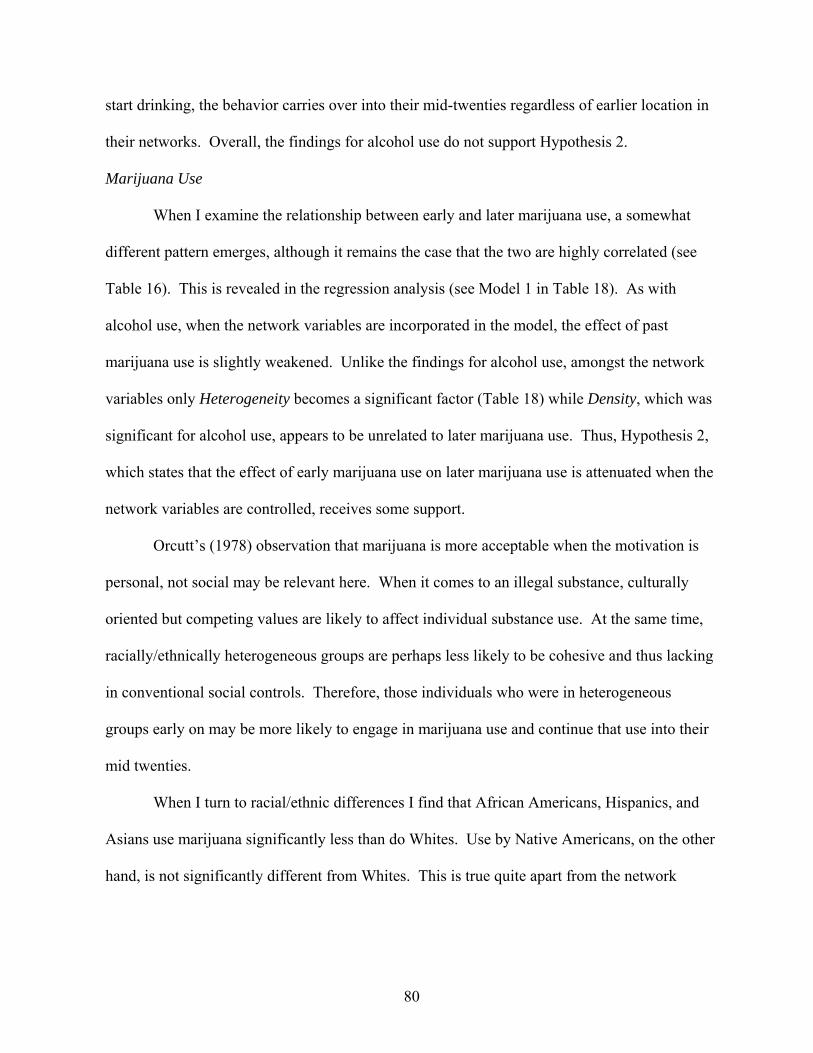
80
start drinking, the behavior carries over into their mid-twenties regardless of earlier location in
their networks. Overall, the findings for alcohol use do not support Hypothesis 2.
Marijuana Use
When I examine the relationship between early and later marijuana use, a somewhat
different pattern emerges, although it remains the case that the two are highly correlated (see
Table 16). This is revealed in the regression analysis (see Model 1 in Table 18). As with
alcohol use, when the network variables are incorporated in the model, the effect of past
marijuana use is slightly weakened. Unlike the findings for alcohol use, amongst the network
variables only Heterogeneity becomes a significant factor (Table 18) while Density, which was
significant for alcohol use, appears to be unrelated to later marijuana use. Thus, Hypothesis 2,
which states that the effect of early marijuana use on later marijuana use is attenuated when the
network variables are controlled, receives some support.
Orcutt’s (1978) observation that marijuana is more acceptable when the motivation is
personal, not social may be relevant here. When it comes to an illegal substance, culturally
oriented but competing values are likely to affect individual substance use. At the same time,
racially/ethnically heterogeneous groups are perhaps less likely to be cohesive and thus lacking
in conventional social controls. Therefore, those individuals who were in heterogeneous
groups early on may be more likely to engage in marijuana use and continue that use into their
mid twenties.
When I turn to racial/ethnic differences I find that African Americans, Hispanics, and
Asians use marijuana significantly less than do Whites. Use by Native Americans, on the other
hand, is not significantly different from Whites. This is true quite apart from the network
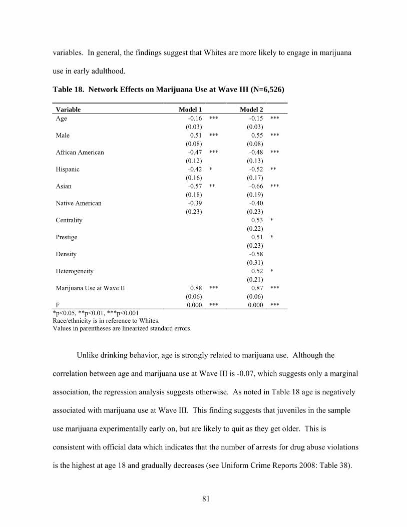
81
variables. In general, the findings suggest that Whites are more likely to engage in marijuana
use in early adulthood.
Table 18. Network Effects on Marijuana Use at Wave III (N=6,526)
Variable Model 1 Model 2 Age -0.16 *** -0.15 ***
(0.03) (0.03)
Male 0.51 *** 0.55 ***
(0.08) (0.08)
African American -0.47 *** -0.48 ***
(0.12) (0.13)
Hispanic -0.42 * -0.52 **
(0.16) (0.17)
Asian -0.57 ** -0.66 ***
(0.18) (0.19)
Native American -0.39 -0.40
(0.23) (0.23)
Centrality 0.53 *
(0.22)
Prestige 0.51 *
(0.23)
Density -0.58
(0.31)
Heterogeneity 0.52 *
(0.21)
Marijuana Use at Wave II 0.88 *** 0.87 ***
(0.06) (0.06)
F 0.000 *** 0.000 *** *p<0.05, **p<0.01, ***p<0.001 Race/ethnicity is in reference to Whites. Values in parentheses are linearized standard errors.
Unlike drinking behavior, age is strongly related to marijuana use. Although the
correlation between age and marijuana use at Wave III is -0.07, which suggests only a marginal
association, the regression analysis suggests otherwise. As noted in Table 18 age is negatively
associated with marijuana use at Wave III. This finding suggests that juveniles in the sample
use marijuana experimentally early on, but are likely to quit as they get older. This is
consistent with official data which indicates that the number of arrests for drug abuse violations
is the highest at age 18 and gradually decreases (see Uniform Crime Reports 2008: Table 38).
82
As with drinking, differences by sex emerge in terms of marijuana use with males being more
likely than females to be users.
Drinking Related Problems
Hypothesis 2 also states that the effect of early alcohol use is diminished when the
network variables are controlled. Two measures of problem drinking are examined: binge
drinking and negative experiences caused by drinking. As reported in Table 19, early alcohol
use has a significant positive effect on later binge drinking. However, the findings in Table 20
suggest that this relationship does not hold for Native Americans.18 As already noted, one
possible explanation for this is that Native Americans are able to cope with adverse situations
as they grow older.
Table 19. The Effect of Early Alcohol Use on Binge Drinking at Wave III
Variable Coefficient Age -0.11 *** 0.03 Male 0.88 *** 0.06 Drinking at Wave II 0.34 *** 0.02 F 0.000 ***
*p<0.05, **p<0.01, ***p<0.001 Values in parentheses are linearized standard errors.
Consistent with expectations, the results show those individuals who engaged in
underage drinking during their teens are more likely to develop binge drinking later on and that
this can be predicted by one’s location in early friendship networks. When network variables
are incorporated into the analysis (see Table 21), the effect of early alcohol use becomes
weaker although it is still significant. That is, the network variables appear to attenuate the
18 The low level of significance is no doubt due to the small sample size. A coefficient of this magnitude would be statistically significant with a larger N.
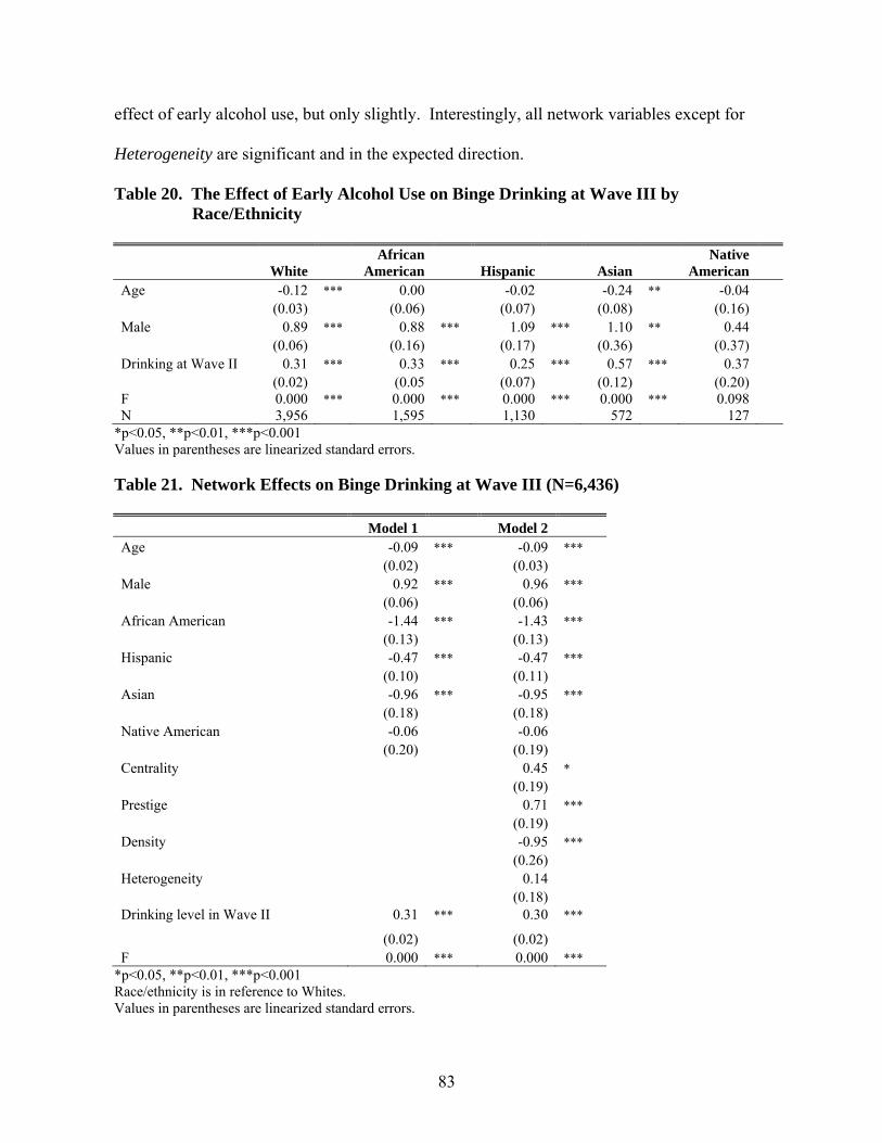
83
effect of early alcohol use, but only slightly. Interestingly, all network variables except for
Heterogeneity are significant and in the expected direction.
Table 20. The Effect of Early Alcohol Use on Binge Drinking at Wave III by Race/Ethnicity
White African
American
Hispanic
Asian Native
American Age -0.12 *** 0.00 -0.02 -0.24 ** -0.04 (0.03) (0.06) (0.07) (0.08) (0.16) Male 0.89 *** 0.88 *** 1.09 *** 1.10 ** 0.44 (0.06) (0.16) (0.17) (0.36) (0.37) Drinking at Wave II 0.31 *** 0.33 *** 0.25 *** 0.57 *** 0.37 (0.02) (0.05 (0.07) (0.12) (0.20) F 0.000 *** 0.000 *** 0.000 *** 0.000 *** 0.098 N 3,956 1,595 1,130 572 127
*p<0.05, **p<0.01, ***p<0.001 Values in parentheses are linearized standard errors. Table 21. Network Effects on Binge Drinking at Wave III (N=6,436)
Model 1 Model 2 Age -0.09 *** -0.09 ***
(0.02) (0.03)
Male 0.92 *** 0.96 ***
(0.06) (0.06)
African American -1.44 *** -1.43 ***
(0.13) (0.13)
Hispanic -0.47 *** -0.47 ***
(0.10) (0.11)
Asian -0.96 *** -0.95 ***
(0.18) (0.18)
Native American -0.06 -0.06
(0.20) (0.19)
Centrality 0.45 *
(0.19)
Prestige 0.71 ***
(0.19)
Density -0.95 ***
(0.26)
Heterogeneity 0.14
(0.18) Drinking level in Wave II 0.31 *** 0.30 ***
(0.02) (0.02)
F 0.000 *** 0.000 *** *p<0.05, **p<0.01, ***p<0.001 Race/ethnicity is in reference to Whites. Values in parentheses are linearized standard errors.

84
As already noted the earlier results suggest that Centrality and Prestige are facilitating
factors while Density is a constraining factor. Individuals who actively nominated others as
friends and were popular while in high school are more likely to drink heavily later on.
Adolescents who were in cohesive groups are less likely to engage in binge drinking later
apparently due to relatively strong conventional social controls. This can no doubt be
explained by their attachment to conventional peers. Cohesiveness represents a collective
effort to produce conformity to conventional expectations.
With regard to race/ethnicity, when all other variables are controlled Whites are more
likely to engage in binge drinking at Wave III (see Table 21). The levels of binge drinking
among all other race/ethnicity groups are significantly lower than the levels for Whites. Whites
are also more likely to be members of racially/ethnically homogeneous groups. However, once
the level of Heterogeneity is controlled, Whites in heterogeneous groups are more likely to
drink.
It is also apparent that males are more likely to engage in binge drinking. The mean
values of binge drinking for males and females, which are related to network variables, are 1.64
and 0.89 respectively. The t-value is 21.19, which is statistically significant (p<0.001, output
not presented).
The findings in Table 22 reveal that underage drinking is positively associated with
alcohol-related problems in early adulthood. Consistent with expectations, youth who engaged
in underage drinking during adolescence are more likely to experience problems caused by
drinking in their mid-twenties. However, unlike binge drinking, all racial/ethnic groups show a
significant positive relationship between early alcohol use and later alcohol-related problems
(see Table 23). The findings in Table 24 suggest that when the network variables are

85
incorporated, the effect of early drinking behavior on problems caused by drinking is weakened,
but again only slightly. Not surprisingly, as with binge drinking, the effects of all of the
network variables other than Heterogeneity are significant.
Table 22. The Effect of Early Alcohol Use on Alcohol-Related Problems at Wave III (N=7,404)
Variable Coefficient Age -0.10 ** 0.03 Male 0.58 *** 0.07 Drinking at Wave II 0.37 *** 0.03 F 0.000 ***
*p<0.05, **p<0.01, ***p<0.001 Values in parentheses are linearized standard errors.
Table 23. The Effect of Early Alcohol Use on Alcohol-Related Problems at Wave III by Race/Ethnicity
African Native White American Hispanic Asian American Age -0.11 ** -0.03 0.02 -0.16 * -0.06 (0.04) (0.05) (0.07) (0.08) (0.15) Male 0.50 *** 0.58 *** 0.92 *** 0.99 ** 0.57 (0.08) (0.15) (0.16) (0.34) (0.41) Drinking at Wave II 0.35 *** 0.30 *** 0.22 * 0.71 *** 0.76 ***
(0.03) (0.07) (0.08) (0.11) (0.19)
F 0.000 *** 0.000 *** 0.000 *** 0.000 *** 0.000 ***
N 3,966 1,597 1,141 574 121 *p<0.05, **p<0.01, ***p<0.001 Values in parentheses are linearized standard errors.
Centrality and Prestige serve as facilitating factors whereas Density functions as a
constraining factor. Males are more likely to experience problems associated with drinking
than females, and age is negatively associated with problems associated with by drinking at
Wave III. Although age is not a significant factor for drinking in general, perhaps because
drinking after age 21 is no longer prohibited, it is negatively associated with problem drinking.
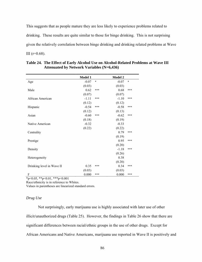
86
This suggests that as people mature they are less likely to experience problems related to
drinking. These results are quite similar to those for binge drinking. This is not surprising
given the relatively correlation between binge drinking and drinking related problems at Wave
III (r=0.68).
Table 24. The Effect of Early Alcohol Use on Alcohol-Related Problems at Wave III Attenuated by Network Variables (N=6,436)
Model 1 Model 2
Age -0.07 * -0.07 *
(0.03) (0.03)
Male 0.62 *** 0.68 ***
(0.07) (0.07)
African American -1.11 *** -1.10 ***
(0.12) (0.12)
Hispanic -0.54 *** -0.58 ***
(0.12) (0.13)
Asian -0.60 *** -0.62 ***
(0.18) (0.19)
Native American -0.32 -0.33
(0.22) (0.22)
Centrality 0.79 ***
(0.19)
Prestige 0.95 ***
(0.20)
Density -1.18 ***
(0.26)
Heterogeneity 0.38
(0.20)
Drinking level in Wave II 0.35 *** 0.34 ***
(0.03) (0.03)
F 0.000 *** 0.000 *** *p<0.05, **p<0.01, ***p<0.001 Race/ethnicity is in reference to Whites. Values in parentheses are linearized standard errors. Drug Use
Not surprisingly, early marijuana use is highly associated with later use of other
illicit/unauthorized drugs (Table 25). However, the findings in Table 26 show that there are
significant differences between racial/ethnic groups in the use of other drugs. Except for
African Americans and Native Americans, marijuana use reported in Wave II is positively and

87
significantly associated with illicit/unauthorized drug use in Wave III. How the effect of early
marijuana use on other illegal/unauthorized drug use is attenuated by the network variables is
examined in Table 27.
Table 25. The Effect of Early Marijuana Use on Other Drug Use at Wave III (N=7,659)
Variable Coefficient
Age -0.13 ***
(0.03)
Male 0.39 ***
(0.07)
Level of marijuana use at Wave II 0.89 ***
(0.06)
F 0.000 *** *p<0.05, **p<0.01, ***p<0.001 Values in parentheses are linearized standard errors.
Table 26. The Effect of Early Marijuana Use on Other Drug Use at Wave III by Race/Ethnicity
White African
American
Hispanic
Asian Native
American Age -0.15 *** -0.03 0.05 -0.29 ** -0.33 *
(0.04) (0.05) (0.07) (0.09) (0.17)
Male 0.46 *** 0.12 0.26 0.40 0.57
(0.09) (0.20) (0.20) (0.28) (0.54)
Marijuana Use at Wave II 0.97 *** 0.15 1.04 *** 0.97 *** 0.53
(0.06) (0.14) (0.14) (0.26) (0.39) F 0.000 *** 0.5123 0.000 *** 0.000 *** 0.1285 N 4,075 1,680 1,173 600 121
*p<0.05, **p<0.01, ***p<0.001 Values in parentheses are linearized standard errors.
As expected, it appears that the network variables tend to attenuate the effect of early
marijuana use on illicit/unauthorized drug use in one’s mid-twenties. When I focus on the
effect of early marijuana use in Model 1, males are more likely to engage in illicit/unauthorized
drug use. With regard to racial/ethnic differences, African Americans and Hispanics
experience illicit/unauthorized drug use significantly less than Whites, but Asians and Native
Americans are not significantly different from Whites.

88
Table 27. Network Effects on Other Drug Use at Wave III (N=6,436)
Model 1 Model 2 Age -0.12 *** -0.12 ***
(0.03) (0.03)
Male 0.39 *** 0.37 ***
(0.08) (0.08)
African American -0.93 *** -0.98 ***
(0.10) (0.10)
Hispanic -0.36 ** -0.50 ***
(0.12) (0.14)
Asian -0.39 * -0.49 **
(0.18) (0.19)
Native American 0.1 -0.01
(0.25) (0.25)
Centrality -0.05
(0.23)
Prestige 0.15
(0.21)
Density -0.11
(0.31)
Heterogeneity 0.52 *
(0.21)
Marijuana Use at Wave II 0.87 *** 0.86 ***
(0.06) (0.06)
F 0.000 *** 0.000 *** *p<0.05, **p<0.01, ***p<0.001 Race/ethnicity is in reference to Whites. Values in parentheses are linearized standard errors.
When the network variables are incorporated into the general model, not only do they
attenuate the effect of early marijuana use, but unlike alcohol related problems only
Heterogeneity appears to be a significantly related to the use of illegal drugs. The tendency for
adolescents in racially heterogeneous groups to accept different opinions from their own may
result in engaging in drug use rather than rejecting use in the future. A lack of cohesiveness in
racially/ethnically heterogeneous groups suggests an absence of conventional social control,
which may in turn facilitate drug use if the actors adopt new value systems to which they have
been exposed.
When Heterogeneity is controlled, Asians exhibit significantly lower
illicit/unauthorized drug involvement than Whites. For Asians, Heterogeneity may weaken

89
group cohesiveness or control resulting in a greater likelihood of illicit/unauthorized drug use.
Since Asians consist of only 4.35 percent of total population in the United States according to
population estimates by the U.S. Census Bureau in 2008, it might be a rare for them to belong
to homogeneous groups in natural social settings except for certain cities where the population
of Asians is high. Thus, any kind of socialization for them is likely to be in heterogeneous
setting. This explanation is based on the racial/ethnic composition in the United States and
similar to the one given for Native Americans given for alcohol use. Due to racial/ethnic
composition in the United States, Asians exhibit significantly lower drug use experience than
Whites when Heterogeneity is set equal. This may be because Asians are less susceptible to
diverse situations and conformity to conventional social norms that may be weakened in a
heterogeneous setting.
In general, Hypothesis 2 is supported by the data. As expected, early network
characteristics appear to attenuate the relationship between early substance use and later
substance use. In fact, how individuals are enmeshed into a group in their adolescent years
seems to have greater long-term compared to short-term effect. In other words, there is some
evidence that network characteristics that develop during the adolescent years carry over into
the respondents’ early adult years. However, there are some differences by substance type.
With regard to alcohol use, Centrality and Prestige have positive long-term effects
while Density tends to have a long-term negative effect. Heterogeneity on the other hand
appears to be unrelated to alcohol use. However, Heterogeneity does show a positive effect for
marijuana and other drug use. In one’s mid-twenties, alcohol use appears to be associated with
popularity while marijuana/other drugs are used among those who are in heterogeneous groups

90
that are assumed to be less cohesive. This suggests that marijuana/other drug users are likely to
engage in such behaviors independently regardless of early friendship networks.
Hypothesis 3
Here I examine whether multiple and meaningful pathways exist in terms of changes in
the level of substance use among youth. Hypothesis 3 states that due to different legal
definitions for alcohol and marijuana use, many will begin to use alcohol and some will
increase their levels of use while the number of marijuana users is likely to decrease as youth
move into adulthood and have more to lose by getting caught.
As already noted, early substance use is associated with later substance use. When the
relationship between early and later substance use is examined by race/ethnicity, the findings in
Tables 28 and 29 reveal that early alcohol use is positively associated with later use across all
race/ethnic groups. Since alcohol is a legal substance and by Wave III the majority of
respondents are no longer minors, this progression is to be expected. On the other hand,
marijuana is an illegal substance regardless of age. Nevertheless, early marijuana use is also
positively associated with later use over the five to six year span between Waves II and III. In
general, the regression analysis shows a positive association between early and later alcohol
and marijuana use. However, I cannot address levels of use or behavioral change until
examining trajectories over time.
Below a one-trajectory growth curve is shown using an unconditional analysis that
specifies the model without a predictor variable (see Figure 2). Because the interval of three
waves is not equidistant, specific commands are given to adjust such differences when the M-
Plus software is used. The same analysis is processed from two- to five-trajectories models to

91
determine the number of trajectories that provides the best fit with the data. The model fitting
statistics for each trajectory-model are presented in Table 30.
Table 28. The Effect of Alcohol Use at Wave II on Alcohol Use at Wave III by Race/Ethnicity
Variable
White African
American
Hispanic
Asian Native
American
Age 0.00 0.03 -0.01 -0.11 0.00
(0.03) (0.05) (0.06) (0.07) (0.15)
Sex 0.66 *** 0.44 *** 0.87 *** 0.91 ** 0.00
(0.07) (0.13) (0.15) (0.29) (0.34)
Alcohol Use at Wave II 0.34 *** 0.35 *** 0.29 *** 0.51 *** 0.35 *
(0.03) (0.05) (0.06) (0.13) (0.18)
F 0.000 *** 0.000 *** 0.000 *** 0.000 *** 0.264 *p<0.05, **p<0.01, ***p<0.001 The values are regression coefficients of alcohol use at Wave II on alcohol use at Wave III for each variable. Values in parentheses are linearized standard errors.
Table 29. The Effect of Marijuana Use at Wave II on Marijuana Use at Wave III by Race/Ethnicity
Variable
White African American
Hispanic
Asian
Native American
Age -0.16 *** -0.13 * -0.09 -0.30 * -0.44 *
(0.03) (0.06) (0.09) (0.12) (0.19)
Sex 0.49 *** 0.65 *** 0.27 0.74 0.20
(0.10) (0.18) (0.22) (0.40) (0.54)
Marijuana use at Wave II 0.85 *** 1.09 *** 0.94 *** 1.45 *** 1.06 **
(0.07) (0.14) (0.15) (0.28) (0.35)
F 0.000 *** 0.000 *** 0.000 *** 0.000 *** 0.001 *** *p<0.05, **p<0.01, ***p<0.001 The values are regression coefficients of marijuana use at Wave II on marijuana use at Wave III for each variable. Values in parentheses are linearized standard errors.
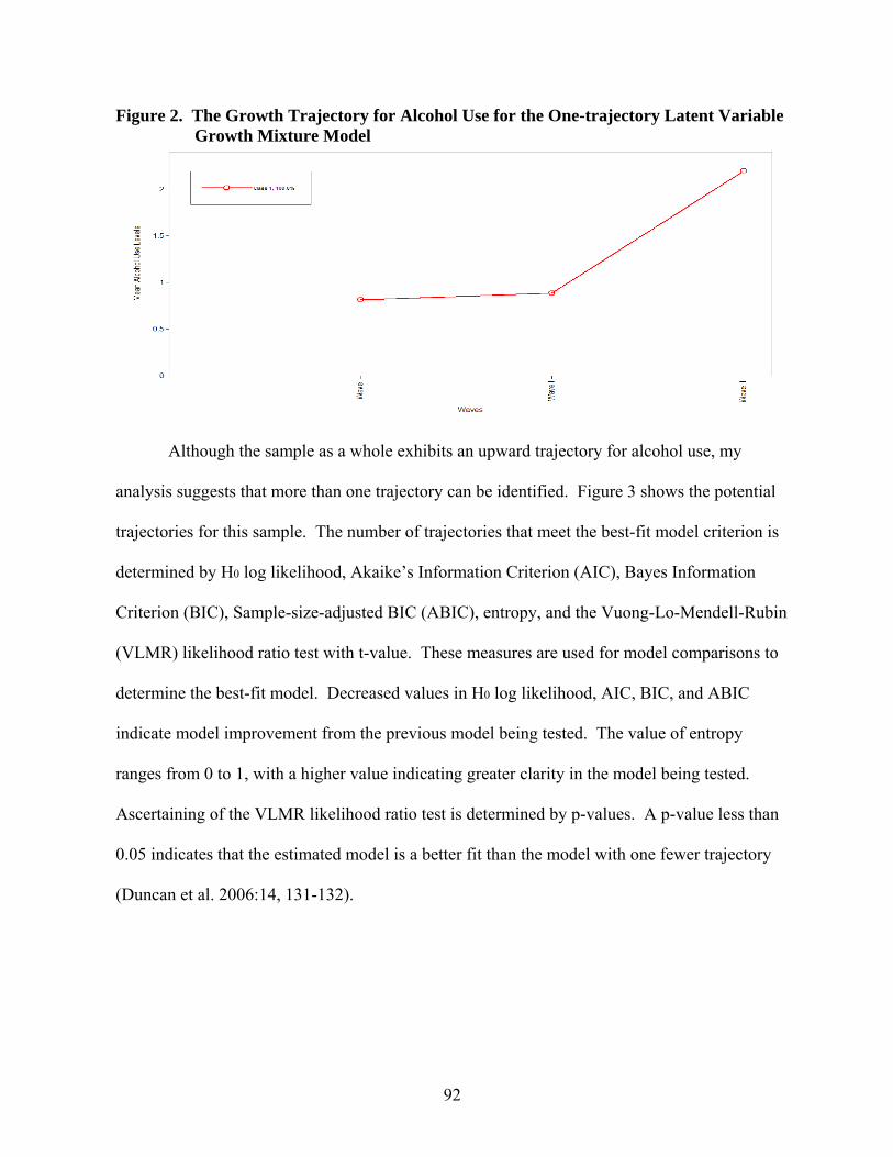
92
Figure 2. The Growth Trajectory for Alcohol Use for the One-trajectory Latent Variable Growth Mixture Model
Although the sample as a whole exhibits an upward trajectory for alcohol use, my
analysis suggests that more than one trajectory can be identified. Figure 3 shows the potential
trajectories for this sample. The number of trajectories that meet the best-fit model criterion is
determined by H0 log likelihood, Akaike’s Information Criterion (AIC), Bayes Information
Criterion (BIC), Sample-size-adjusted BIC (ABIC), entropy, and the Vuong-Lo-Mendell-Rubin
(VLMR) likelihood ratio test with t-value. These measures are used for model comparisons to
determine the best-fit model. Decreased values in H0 log likelihood, AIC, BIC, and ABIC
indicate model improvement from the previous model being tested. The value of entropy
ranges from 0 to 1, with a higher value indicating greater clarity in the model being tested.
Ascertaining of the VLMR likelihood ratio test is determined by p-values. A p-value less than
0.05 indicates that the estimated model is a better fit than the model with one fewer trajectory
(Duncan et al. 2006:14, 131-132).
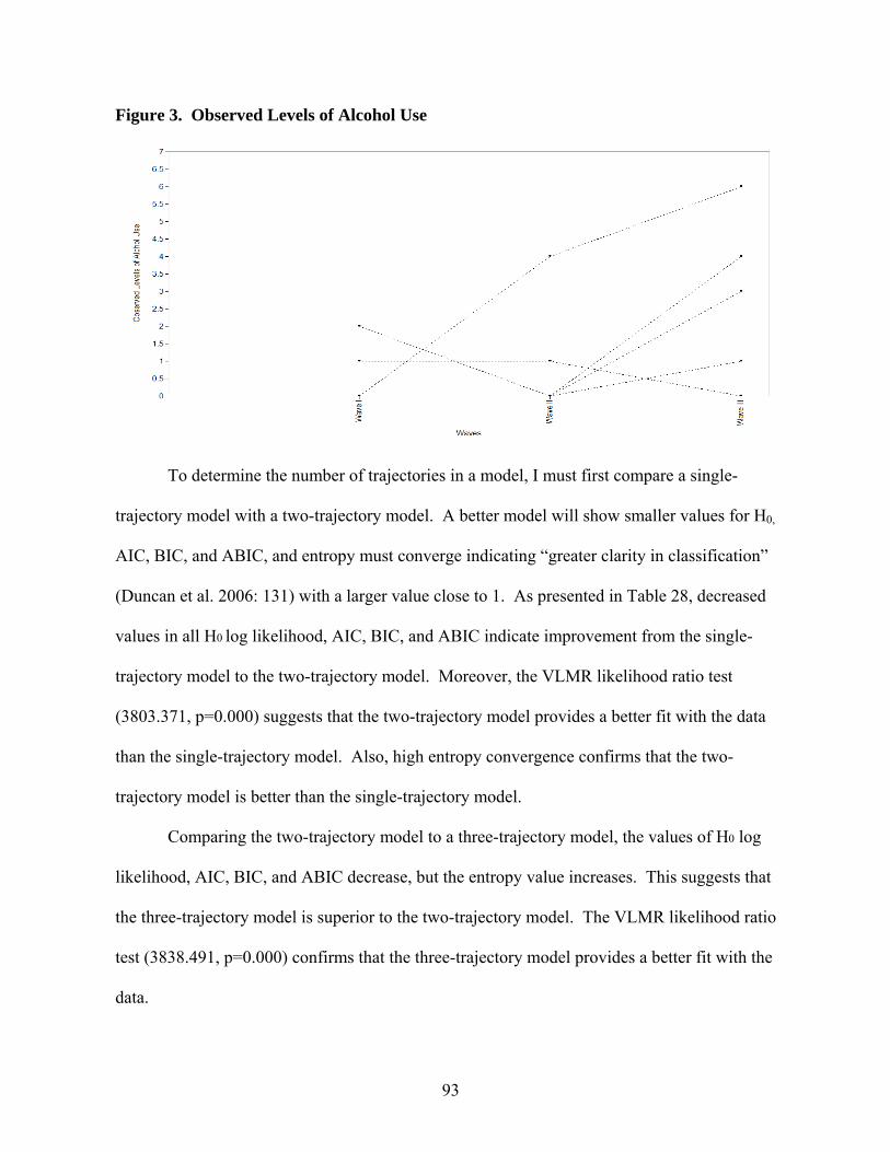
93
Figure 3. Observed Levels of Alcohol Use
To determine the number of trajectories in a model, I must first compare a single-
trajectory model with a two-trajectory model. A better model will show smaller values for H0,
AIC, BIC, and ABIC, and entropy must converge indicating “greater clarity in classification”
(Duncan et al. 2006: 131) with a larger value close to 1. As presented in Table 28, decreased
values in all H0 log likelihood, AIC, BIC, and ABIC indicate improvement from the single-
trajectory model to the two-trajectory model. Moreover, the VLMR likelihood ratio test
(3803.371, p=0.000) suggests that the two-trajectory model provides a better fit with the data
than the single-trajectory model. Also, high entropy convergence confirms that the two-
trajectory model is better than the single-trajectory model.
Comparing the two-trajectory model to a three-trajectory model, the values of H0 log
likelihood, AIC, BIC, and ABIC decrease, but the entropy value increases. This suggests that
the three-trajectory model is superior to the two-trajectory model. The VLMR likelihood ratio
test (3838.491, p=0.000) confirms that the three-trajectory model provides a better fit with the
data.
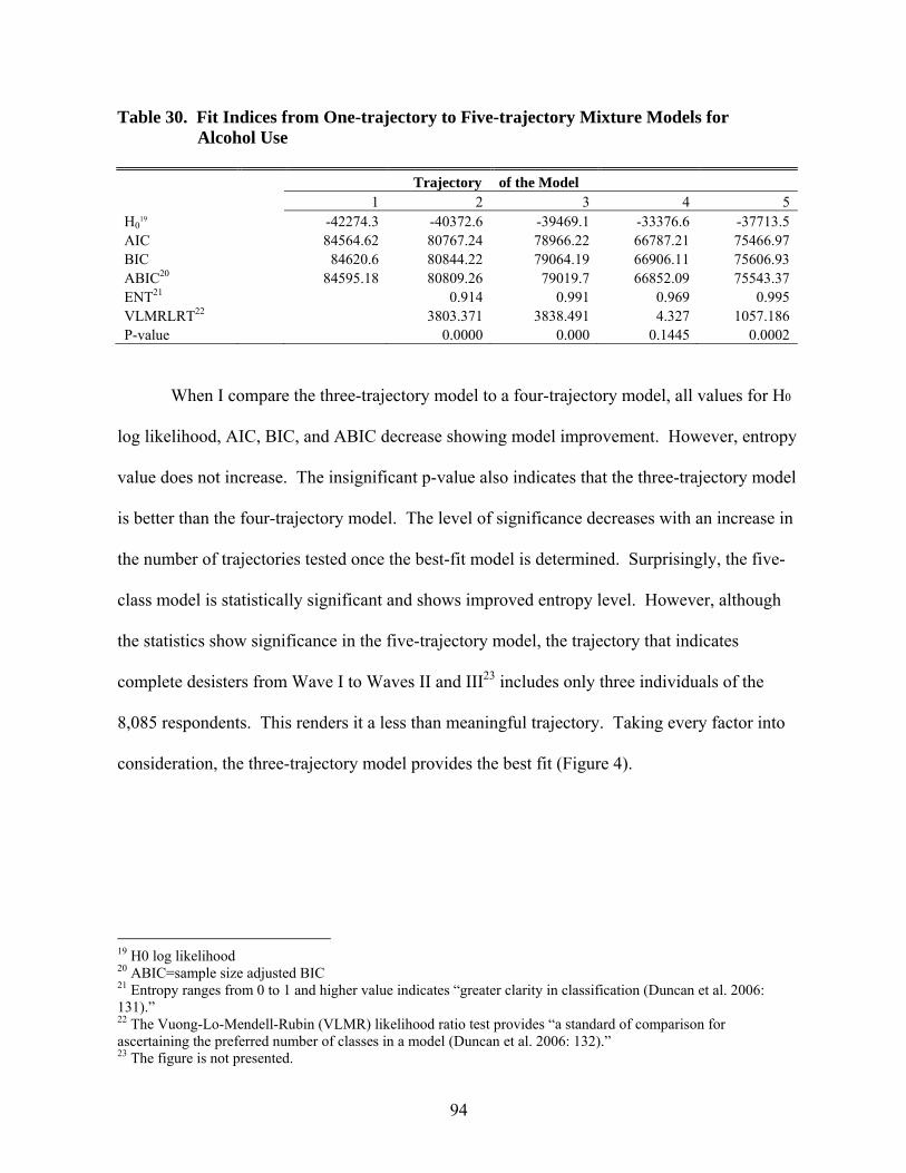
94
Table 30. Fit Indices from One-trajectory to Five-trajectory Mixture Models for Alcohol Use
Trajectory of the Model 1 2 3 4 5 H0
19 -42274.3 -40372.6 -39469.1 -33376.6 -37713.5 AIC 84564.62 80767.24 78966.22 66787.21 75466.97 BIC 84620.6 80844.22 79064.19 66906.11 75606.93 ABIC20 84595.18 80809.26 79019.7 66852.09 75543.37 ENT21 0.914 0.991 0.969 0.995 VLMRLRT22 3803.371 3838.491 4.327 1057.186 P-value 0.0000 0.000 0.1445 0.0002
When I compare the three-trajectory model to a four-trajectory model, all values for H0
log likelihood, AIC, BIC, and ABIC decrease showing model improvement. However, entropy
value does not increase. The insignificant p-value also indicates that the three-trajectory model
is better than the four-trajectory model. The level of significance decreases with an increase in
the number of trajectories tested once the best-fit model is determined. Surprisingly, the five-
class model is statistically significant and shows improved entropy level. However, although
the statistics show significance in the five-trajectory model, the trajectory that indicates
complete desisters from Wave I to Waves II and III23 includes only three individuals of the
8,085 respondents. This renders it a less than meaningful trajectory. Taking every factor into
consideration, the three-trajectory model provides the best fit (Figure 4).
19 H0 log likelihood 20 ABIC=sample size adjusted BIC 21 Entropy ranges from 0 to 1 and higher value indicates “greater clarity in classification (Duncan et al. 2006: 131).” 22 The Vuong-Lo-Mendell-Rubin (VLMR) likelihood ratio test provides “a standard of comparison for ascertaining the preferred number of classes in a model (Duncan et al. 2006: 132).” 23 The figure is not presented.
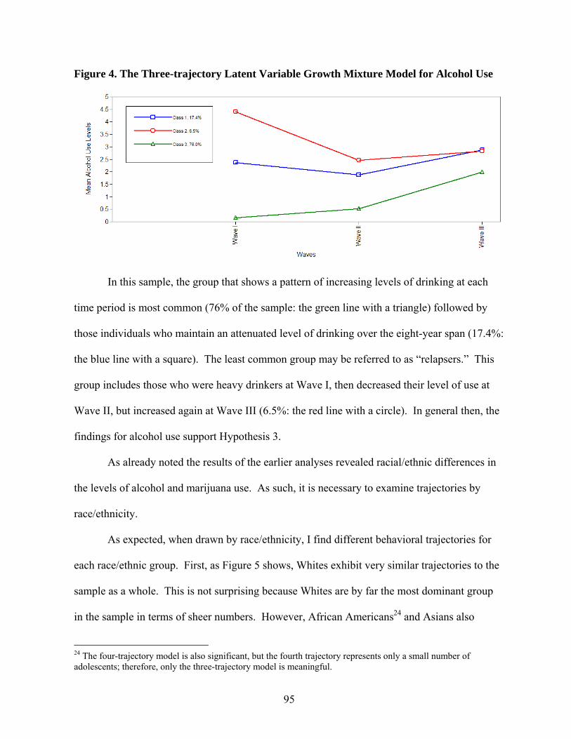
95
Figure 4. The Three-trajectory Latent Variable Growth Mixture Model for Alcohol Use
In this sample, the group that shows a pattern of increasing levels of drinking at each
time period is most common (76% of the sample: the green line with a triangle) followed by
those individuals who maintain an attenuated level of drinking over the eight-year span (17.4%:
the blue line with a square). The least common group may be referred to as “relapsers.” This
group includes those who were heavy drinkers at Wave I, then decreased their level of use at
Wave II, but increased again at Wave III (6.5%: the red line with a circle). In general then, the
findings for alcohol use support Hypothesis 3.
As already noted the results of the earlier analyses revealed racial/ethnic differences in
the levels of alcohol and marijuana use. As such, it is necessary to examine trajectories by
race/ethnicity.
As expected, when drawn by race/ethnicity, I find different behavioral trajectories for
each race/ethnic group. First, as Figure 5 shows, Whites exhibit very similar trajectories to the
sample as a whole. This is not surprising because Whites are by far the most dominant group
in the sample in terms of sheer numbers. However, African Americans24 and Asians also
24 The four-trajectory model is also significant, but the fourth trajectory represents only a small number of adolescents; therefore, only the three-trajectory model is meaningful.
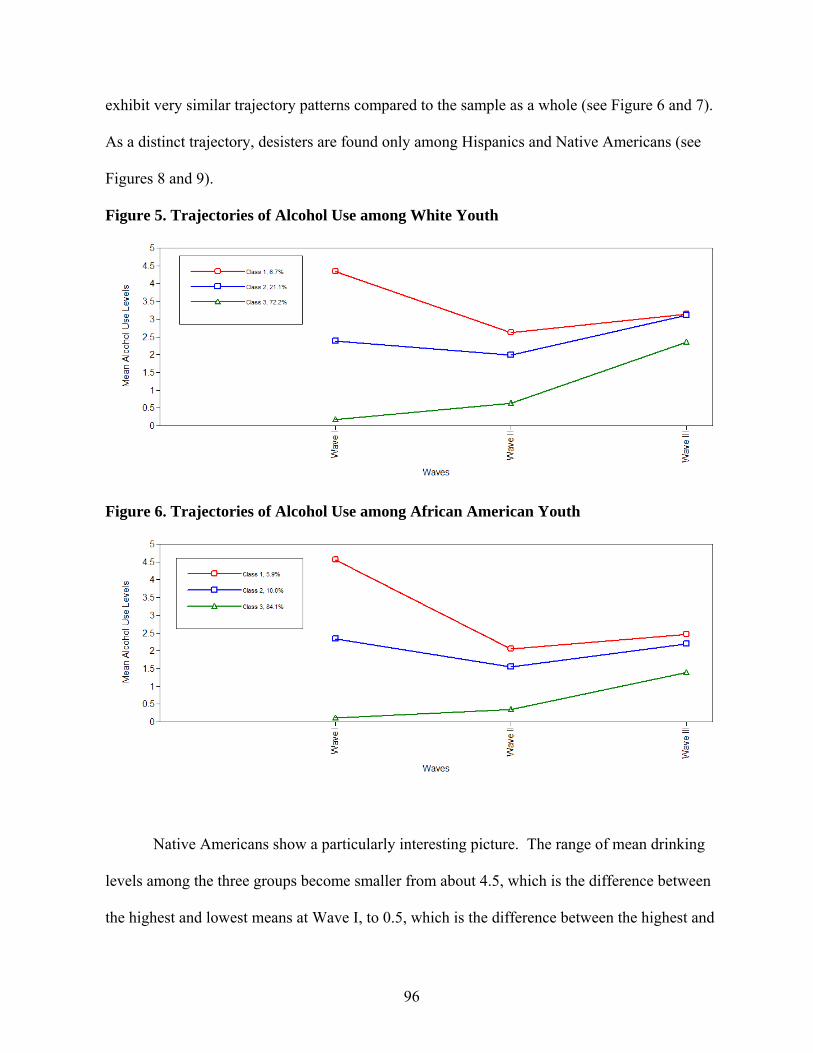
96
exhibit very similar trajectory patterns compared to the sample as a whole (see Figure 6 and 7).
As a distinct trajectory, desisters are found only among Hispanics and Native Americans (see
Figures 8 and 9).
Figure 5. Trajectories of Alcohol Use among White Youth
Figure 6. Trajectories of Alcohol Use among African American Youth
Native Americans show a particularly interesting picture. The range of mean drinking
levels among the three groups become smaller from about 4.5, which is the difference between
the highest and lowest means at Wave I, to 0.5, which is the difference between the highest and

97
lowest means at Wave III. That is, their drinking behavior became extremely similar at Wave
III. In the three-trajectory model, Native American youth who exhibit the lowest levels of
drinking at Wave I pass over the levels of the other two trajectories by Wave III (Figure 9).
The existence of desisters may contribute to the convergence in the drinking level at Wave III.
The levels of marijuana use in the past 30 days at Waves I through III are used to draw
trajectories for marijuana use. The findings reveal that a three-trajectory model provides the
best fit for marijuana use (Table 31 and Figure 10).25 The majority of users (76.6%: the blue
line with a triangle) appear to be experimental users at Wave II and non-users by Wave III.
About one-fourth of the sample (23.1%: the green line with a triangle) show an increase in
marijuana use over time and only a small group of individuals (0.3%: the red line with a circle)
desist from marijuana use over time. As with alcohol use, the findings for marijuana use
provide support for Hypothesis 3.
Figure 7. Trajectories of Alcohol Use among Asian Youth
When examining marijuana use by race/ethnicity, three trajectories were observed only
among Whites (Figure 11). These trajectories appear to account for the three different
25 The model did not converge into four trajectories, but started to do again into five-class trajectories. Although entropy value increased, trajectory 1 and 5 contained only a small number of individuals which resulted in 0.01percenr (6 individuals) and 0.02 percent (16 individuals) of this model.

98
trajectories for the sample as a whole. One group (77.9%: the blue line with a square)
gradually increased their marijuana use while the other (12.8%: the red line with a circle)
slowly decreased the level of marijuana use over time. The final group (9.3%: the green line
with a triangle) exhibits sharp increase in marijuana use over time. This group includes youth
who were non-users at Wave I, then, rapidly increased their use over time. The findings related
to Hypothesis 2 suggested that Heterogeneity in groups is related to an increase in the level of
marijuana use; thus, White individuals who exhibit a decrease in the level of marijuana use are
assumed to be in homogeneous and therefore cohesive groups as they get older.
Figure 8. Trajectories of Alcohol Use among Hispanic Youth
African American and Asian Youth exhibit trajectories consistent with my expectation
(see Figures 12 and 13). Less than 15 percent of each racial group shows progression into
marijuana use. The only difference between African American and Asian Youth is that the
majority of African American youth appear to continue marijuana use at the very low level
over three waves whereas the majority of Asian youth actually desist from marijuana use at
Wave III.
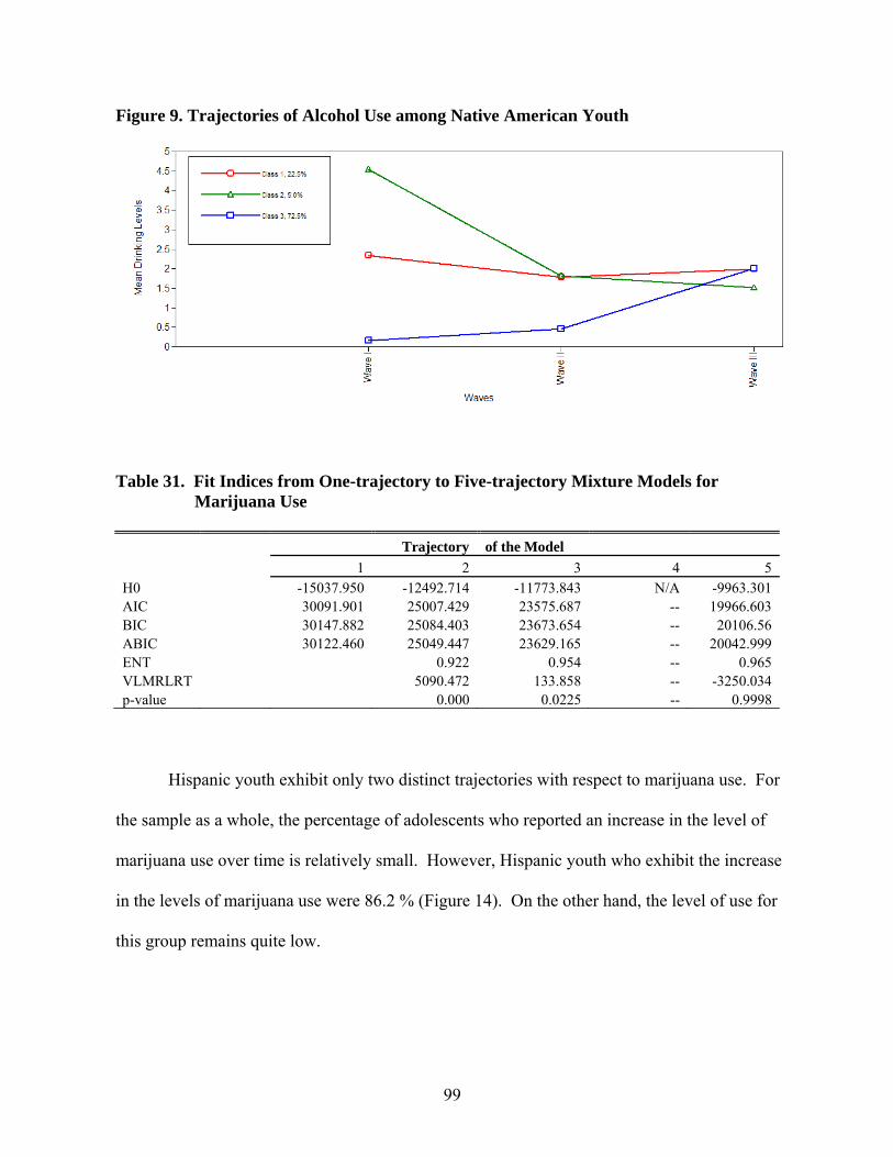
99
Figure 9. Trajectories of Alcohol Use among Native American Youth
Table 31. Fit Indices from One-trajectory to Five-trajectory Mixture Models for Marijuana Use
Trajectory of the Model
1 2 3 4 5 H0 -15037.950 -12492.714 -11773.843 N/A -9963.301 AIC 30091.901 25007.429 23575.687 -- 19966.603 BIC 30147.882 25084.403 23673.654 -- 20106.56 ABIC 30122.460 25049.447 23629.165 -- 20042.999 ENT 0.922 0.954 -- 0.965 VLMRLRT 5090.472 133.858 -- -3250.034 p-value 0.000 0.0225 -- 0.9998
Hispanic youth exhibit only two distinct trajectories with respect to marijuana use. For
the sample as a whole, the percentage of adolescents who reported an increase in the level of
marijuana use over time is relatively small. However, Hispanic youth who exhibit the increase
in the levels of marijuana use were 86.2 % (Figure 14). On the other hand, the level of use for
this group remains quite low.

100
Figure 10. The Three-trajectory Latent Variable Growth Mixture Model for Marijuana Use
Figure 11. Trajectories of Marijuana Use among White Youth
It is also noteworthy that among Native American youth there are two distinct
trajectories (Figure 15). Although these groups show very similar marijuana use level at Wave
I, they eventually take very divergent trajectories: Some become non-users while others
become heavy users by Wave III. As the results relating to Hypotheses 2 revealed,
Heterogeneity in one’s early friendship has a significant positive effect on later marijuana use.
As already noted, Native American youth in this study tend to be in heterogeneous groups.
Thus, although it is not surprising that the Native Americans show an increase in use over time
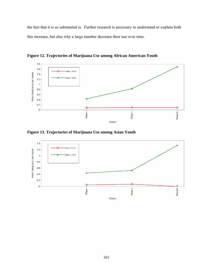
101
the fact that it is so substantial is. Further research is necessary to understand or explain both
this increase, but also why a large number decrease their use over time.
Figure 12. Trajectories of Marijuana Use among African American Youth
Figure 13. Trajectories of Marijuana Use among Asian Youth
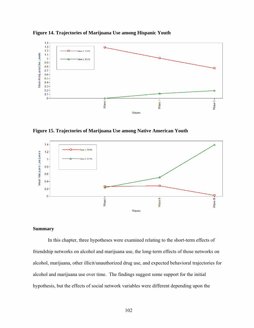
102
Figure 14. Trajectories of Marijuana Use among Hispanic Youth
Figure 15. Trajectories of Marijuana Use among Native American Youth
Summary
In this chapter, three hypotheses were examined relating to the short-term effects of
friendship networks on alcohol and marijuana use, the long-term effects of those networks on
alcohol, marijuana, other illicit/unauthorized drug use, and expected behavioral trajectories for
alcohol and marijuana use over time. The findings suggest some support for the initial
hypothesis, but the effects of social network variables were different depending upon the
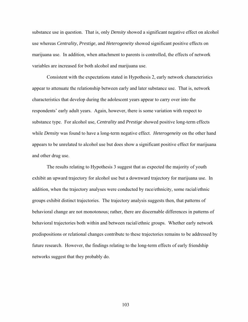
103
substance use in question. That is, only Density showed a significant negative effect on alcohol
use whereas Centrality, Prestige, and Heterogeneity showed significant positive effects on
marijuana use. In addition, when attachment to parents is controlled, the effects of network
variables are increased for both alcohol and marijuana use.
Consistent with the expectations stated in Hypothesis 2, early network characteristics
appear to attenuate the relationship between early and later substance use. That is, network
characteristics that develop during the adolescent years appear to carry over into the
respondents’ early adult years. Again, however, there is some variation with respect to
substance type. For alcohol use, Centrality and Prestige showed positive long-term effects
while Density was found to have a long-term negative effect. Heterogeneity on the other hand
appears to be unrelated to alcohol use but does show a significant positive effect for marijuana
and other drug use.
The results relating to Hypothesis 3 suggest that as expected the majority of youth
exhibit an upward trajectory for alcohol use but a downward trajectory for marijuana use. In
addition, when the trajectory analyses were conducted by race/ethnicity, some racial/ethnic
groups exhibit distinct trajectories. The trajectory analysis suggests then, that patterns of
behavioral change are not monotonous; rather, there are discernable differences in patterns of
behavioral trajectories both within and between racial/ethnic groups. Whether early network
predispositions or relational changes contribute to these trajectories remains to be addressed by
future research. However, the findings relating to the long-term effects of early friendship
networks suggest that they probably do.
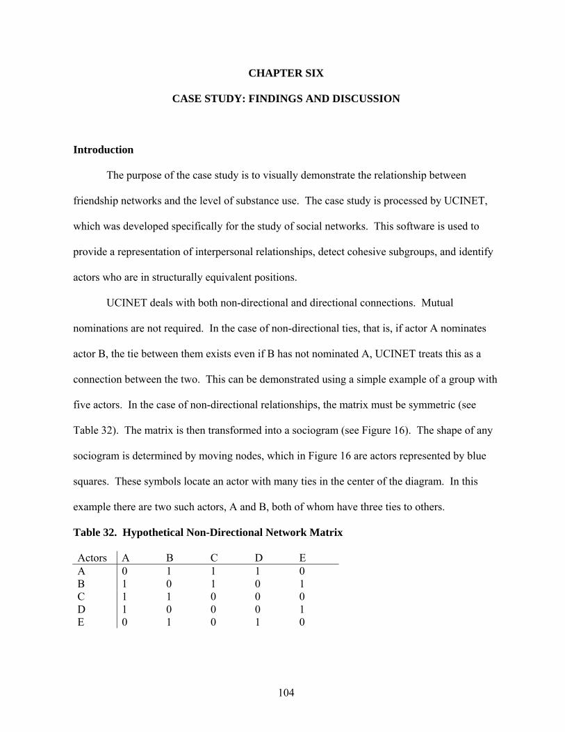
104
CHAPTER SIX
CASE STUDY: FINDINGS AND DISCUSSION
Introduction
The purpose of the case study is to visually demonstrate the relationship between
friendship networks and the level of substance use. The case study is processed by UCINET,
which was developed specifically for the study of social networks. This software is used to
provide a representation of interpersonal relationships, detect cohesive subgroups, and identify
actors who are in structurally equivalent positions.
UCINET deals with both non-directional and directional connections. Mutual
nominations are not required. In the case of non-directional ties, that is, if actor A nominates
actor B, the tie between them exists even if B has not nominated A, UCINET treats this as a
connection between the two. This can be demonstrated using a simple example of a group with
five actors. In the case of non-directional relationships, the matrix must be symmetric (see
Table 32). The matrix is then transformed into a sociogram (see Figure 16). The shape of any
sociogram is determined by moving nodes, which in Figure 16 are actors represented by blue
squares. These symbols locate an actor with many ties in the center of the diagram. In this
example there are two such actors, A and B, both of whom have three ties to others.
Table 32. Hypothetical Non-Directional Network Matrix
Actors A B C D E A 0 1 1 1 0 B 1 0 1 0 1 C 1 1 0 0 0 D 1 0 0 0 1 E 0 1 0 1 0
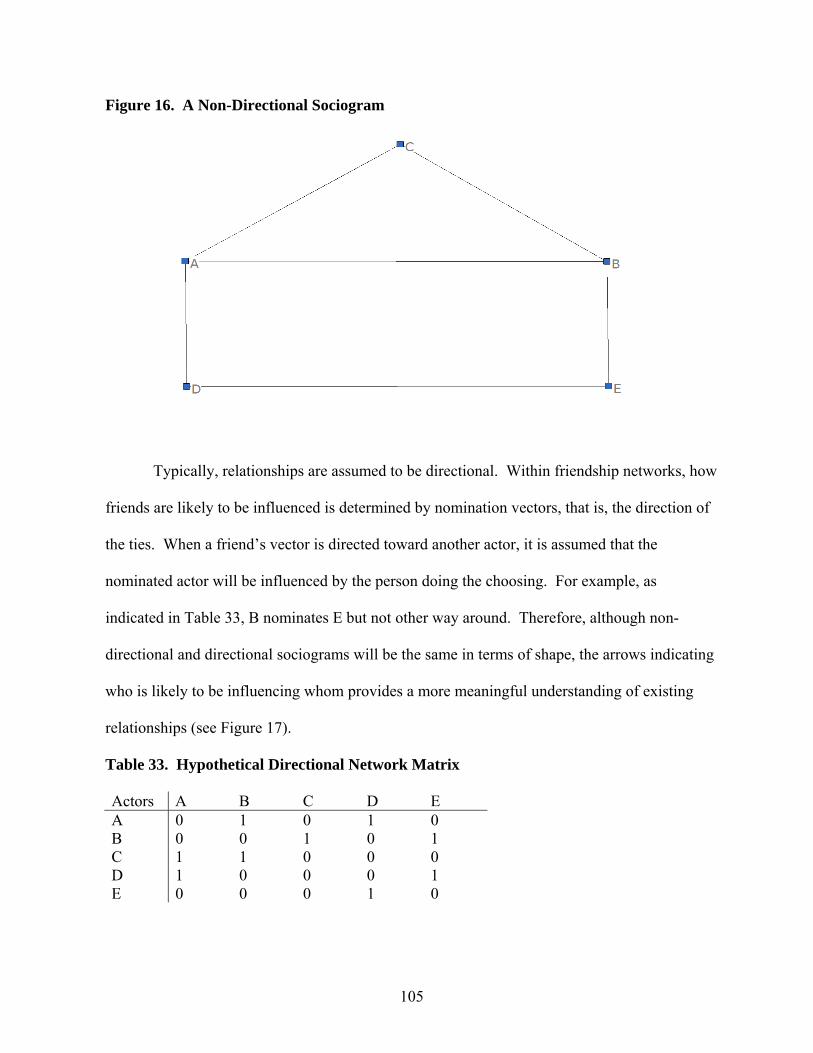
105
Figure 16. A Non-Directional Sociogram
Typically, relationships are assumed to be directional. Within friendship networks, how
friends are likely to be influenced is determined by nomination vectors, that is, the direction of
the ties. When a friend’s vector is directed toward another actor, it is assumed that the
nominated actor will be influenced by the person doing the choosing. For example, as
indicated in Table 33, B nominates E but not other way around. Therefore, although non-
directional and directional sociograms will be the same in terms of shape, the arrows indicating
who is likely to be influencing whom provides a more meaningful understanding of existing
relationships (see Figure 17).
Table 33. Hypothetical Directional Network Matrix
Actors A B C D E A 0 1 0 1 0 B 0 0 1 0 1 C 1 1 0 0 0 D 1 0 0 0 1 E 0 0 0 1 0
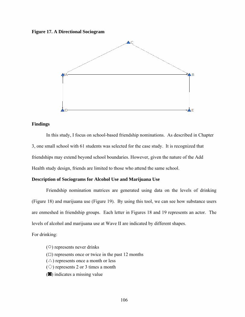
106
Figure 17. A Directional Sociogram
Findings
In this study, I focus on school-based friendship nominations. As described in Chapter
3, one small school with 61 students was selected for the case study. It is recognized that
friendships may extend beyond school boundaries. However, given the nature of the Add
Health study design, friends are limited to those who attend the same school.
Description of Sociograms for Alcohol Use and Marijuana Use
Friendship nomination matrices are generated using data on the levels of drinking
(Figure 18) and marijuana use (Figure 19). By using this tool, we can see how substance users
are enmeshed in friendship groups. Each letter in Figures 18 and 19 represents an actor. The
levels of alcohol and marijuana use at Wave II are indicated by different shapes.
For drinking:
(○) represents never drinks
(□) represents once or twice in the past 12 months (△) represents once a month or less (◇) represents 2 or 3 times a month
(◙) indicates a missing value

107
For marijuana use:
(○) represents never used marijuana
(□) represents low level of use (△) represents high level of marijuana use
(◙) represents missing values
As can be seen in Figures 18 and 19, all students are tied to others except for three who
may be described as social isolates. These three are located in the top left corners of the two
Figures. In general, there are two major groups in this school as illustrated in both diagrams,
and these groups are bridged by one actor U. This person is in a convenient location to
maintain contact with any other student in either of the two groups. In other words, without
this person, the two groups would be separate.
In terms of alcohol use, we can identify one user subgroup on the far left of the diagram
in Figure 18. This group includes actors D, AB, AP, and BA. The sociogram suggests that
alcohol users are likely to be directly linked to other users. The one apparent exception is the
relationship between actors D and AP. These two are indirectly linked through actor AB who
happens to be a non-drinker.
In addition to the above, it should be noted that the mean age of the alcohol users is 16.7
and that two of the three drinkers are female. Because the number of alcohol users is very
small the fact that the larger proportion of female drinkers compared to the quantitative results
is not particularly meaningful. However, the age factor is generally consistent with the
quantitative results, which suggested that older youth may socialize younger youth with regard
to substance use.
For marijuana use, all of the users again appear to be connected to one another. It is
also interesting to note that, as expected there is overlap between the alcohol and marijuana

108
users (Figure 19). This is perhaps understandable because alcohol use is a status offense and
marijuana is illegal for adults. Therefore, marijuana users are more likely to use alcohol than
the other way around. However, it seems clear that in this school substance use is limited to a
small group. It is also noteworthy that there are no extreme users. Rather, all users maintain
similar levels of substance use. This may reflect the small school size, which serves as a source
of conventional control.
The Effects of Network Variables on Alcohol and Marijuana Use
Since the three substance users identified above, that is D, AP, and BA, are in the same
group, the number of directional ties is used to examine Centrality and Prestige without
standardizing by the users’ network size. Among attenuate level alcohol users, that is, actors D,
AP, and BA, neither D nor AP nominated anyone as a friend, but each is appointed as a friend
by other classmates (see Figures 18 or 19). Actor D has four appointed ties and actor AP has
two. Actor BA, who is in close proximity to actors D and AP, nominated four classmates and
received five nominations. Except for actor BA, the proportion of appointing ties over
nominating ties is very high. This consistent with the earlier finding that Centrality, at least as
measured here, is not associated with alcohol use. Also, consistent with the earlier findings, is
the fact that alcohol users tend to be popular as indicated by their high Prestige standing. The
fourth student AB is a non-drinker, but is in a group of alcohol users D, AP, and BA and
nominated all three as friends. Interestingly, none of the alcohol users nominated AB as a
friend.
This group, including AB, seems similar to what Yablonsky (1959: 109) referred to as a
“near group” which is characterized as one in which there is “diffuse role definition, limited
cohesion, shifting membership, or limited definition of membership expectations.” In the near
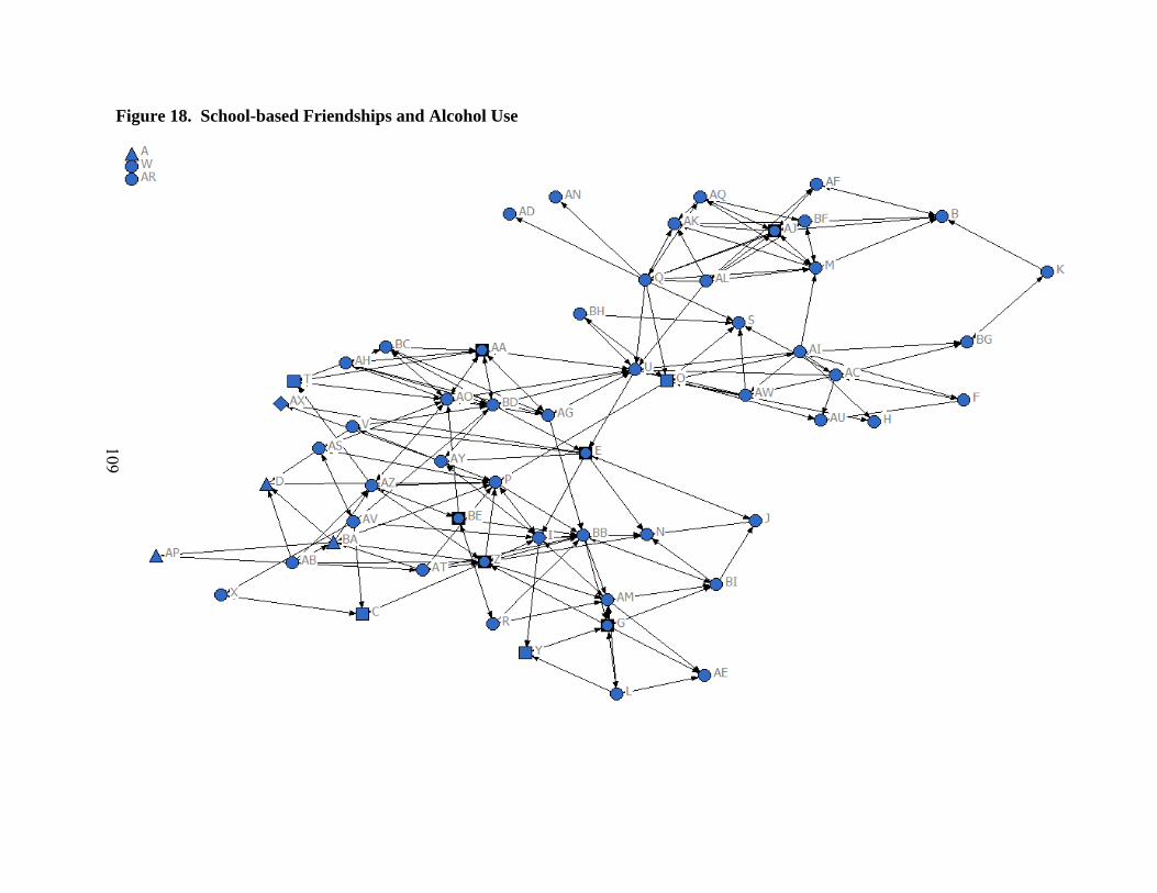
109
Figure 18. School-based Friendships and Alcohol Use
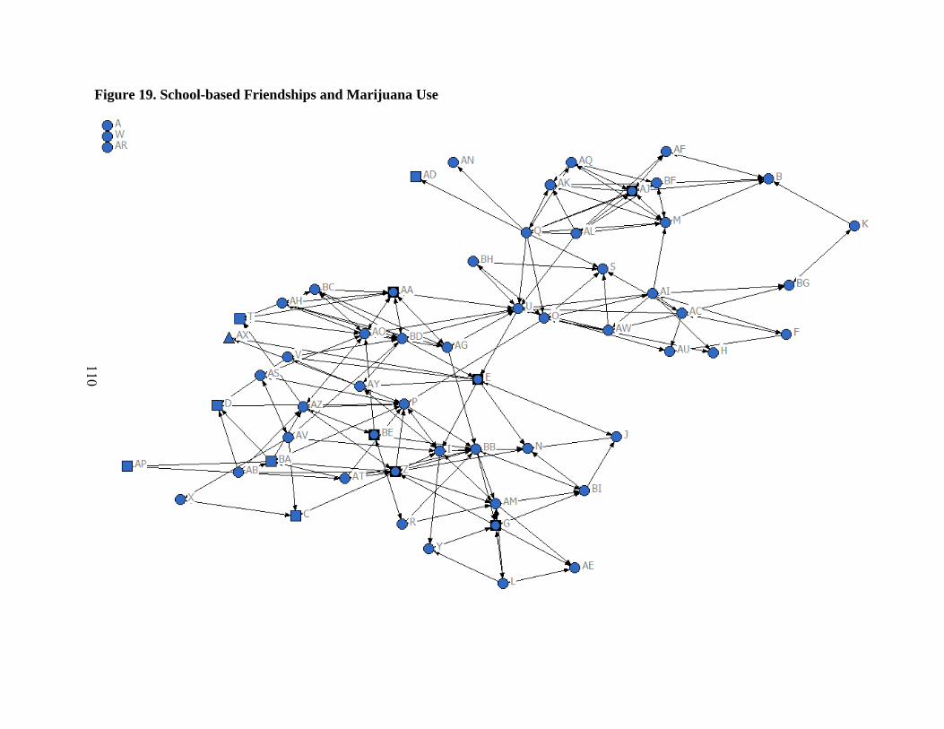
110
Figure 19. School-based Friendships and Marijuana Use

111
group, marginal members are those who “claim affiliation in the gang but only participate in it
according to their emotional needs at given times” or are “never defined by themselves or
others as a gang member.” (113) Actor AB appears to take on this role in this group.
When examining Density, or cohesiveness, using the density measure from the
quantitative study (see Table 34),26 it appears that students who have ever used alcohol or
marijuana show approximately the same density levels as the average for all students in this
school (Mean Density level=0.46).27 For example, the Density level of actor D is 0.5 and for
actor BA it is 0.45. This appears to reflect the results for alcohol use in the quantitative study
although some qualifications are necessary. In the user group, the average level of Density for
actors D, AB, AP, and BA is 0.42 (5/4*(4-1)), which is lower than the average individual
Density levels for all youth attending this school.28 This is again consistent with the results in
the quantitative study, which showed that users are likely to be members of groups that are less
cohesive than most.
Table 34. Network Characteristics Held by Actors
Actors Indegree Outdegree Centrality Prestige Density D 4 0 0 1 0.5 AB 0 6 1 0 0.43
AP (2) BA 5 4 0.57 0.71 0.45
* Blank refers to missing values due to non-participation in the network survey. * The value in parentheses is based on manual counting.
26 The full table, which includes all respondents in the Case Study school, is too large to reproduce here. It is available from the author upon request. 27 Average Density is calculated based on the Density values for each individual. This was calculated as follows: The sum of Density is divided by the number of students. Those who did not participate in the school survey were not included. 28 Because actor AP did not participate in school survey, all four network variables for AP are recorded as missing. However, because the actor AP is appointed as a friend from others, we can count the incoming ties manually as indicated in the parentheses in Table 34.
112
As noted above, there are no extreme substance users in the substance user group.
There are at least two plausible explanations for this. One explanation is that the substance
user group effectively controls the upper limits of use. This involves the notion of socialization
to group norms that place limits on the level of substance use the members will tolerate. An
alternative explanation is that substance users choose as friends others who exhibit similar
levels of substance use. This involves the notion of social selection and suggests that users are
more likely to choose others whose substance use levels are similar to their own. Thus, either
or both selection and socialization effects may account for the absence of extreme users.
As noted in Chapter 3 the Case Study sample includes very few minority students (three
out of 61 students). Therefore, the network variable Heterogeneity cannot be examined.
However, among the substance group members identified above, actor D is Hispanic. Thus,
this user group can be considered to be a heterogeneous group and is consistent with the
findings in the quantitative study although this holds only for marijuana use.
When I turn to the level of attachment to parents, actors D, AB, and BA express
attenuate attachment to their parents, and actor AP reports low attachment (Table 35). The fact
that none of the alcohol and marijuana users express high attachment to parents suggests that
they are less constrained in choosing other substance users as friends. This is also consistent
with Warr’s (1993a) findings that the strength of one’s attachment to parents influences friend
selection. These findings are also consistent with the results from the quantitative study where
I found that high attachment to parents was negatively associated with both alcohol and
marijuana use.
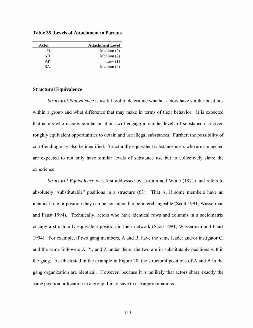
113
Table 35. Levels of Attachment to Parents
Actor Attachment Level D Medium (2)
AB Medium (2) AP Low (1) BA Medium (2)
Structural Equivalence
Structural Equivalence is useful tool to determine whether actors have similar positions
within a group and what difference that may make in terms of their behavior. It is expected
that actors who occupy similar positions will engage in similar levels of substance use given
roughly equivalent opportunities to obtain and use illegal substances. Further, the possibility of
co-offending may also be identified. Structurally equivalent substance users who are connected
are expected to not only have similar levels of substance use but to collectively share the
experience.
Structural Equivalence was first addressed by Lorrain and White (1971) and refers to
absolutely “substitutable” positions in a structure (63). That is, if some members have an
identical role or position they can be considered to be interchangeable (Scott 1991; Wasserman
and Faust 1994). Technically, actors who have identical rows and columns in a sociomatrix
occupy a structurally equivalent position in their network (Scott 1991; Wasserman and Faust
1994). For example, if two gang members, A and B, have the same leader and/or instigator C,
and the same followers X, Y, and Z under them, the two are in substitutable positions within
the gang. As illustrated in the example in Figure 20, the structural positions of A and B in the
gang organization are identical. However, because it is unlikely that actors share exactly the
same position or location in a group, I may have to use approximations.

114
Figure 20. Example of Structural Equivalence
There are several alternative measures of Structural Equivalence, but the most widely
used are Euclidean distance and Pearson correlation. Euclidean distance was developed by
Burt (1976; 1978) and structural equivalence between actors is determined using geodesic
distance, which refers to the shortest path between actors (Wasserman and Faust 1994: 367).
The Euclidean distance is computed for all pairs in the networks. The second measure uses the
“Pearson product-moment” (368) correlation coefficient to determine the degree of similarity
or dissimilarity between every pair of actors. When two actors are structurally equivalent, the
correlation between pairs of actors is +1; when two actors are completely dissimilar the
correlation is -1. When a network is large as is the case here, it is likely that two actors are
located some distance from each other. Therefore, Euclidean distance is not the best measure.
Thus, I have used Pearson correlation.
Since the majority of students in this school are not substance users, I can focus on
similarities in the positions of actors D, AP, and BA, the few substance users identified in the
analysis. The correlations between actors D and AP, D and BA, and AP and BA are 0.7, 0.42,
C
A B
X Y Z X Y Z

115
and 0.37 respectively (see Table 36).29 These correlations are strong enough to suggest
similarity rather than dissimilarity. This is especially true for actors D and AP. The other
substance user pairs D and BA, and AP and BA exhibit similarity, but at somewhat lower level.
Figure 21 illustrates the direct ties among six substance users who engage in both
alcohol and marijuana use and allows us to examine their structural equivalence. For example,
when I compare D to AP I find that both actors are connected through AB and BA. This is one
aspect of the similarity between D and AP. Second, these connections are made based on
nominations from AB and BA. Third, both D and AP do not nominate anyone else. In addition,
and as already noted, the Pearson correlations indicate strong similarity between D and AP
(r=0.70, Table 36). A second example showing similarity involves actors AP and BA. Both are
nominated by AB and the appointed ties overweigh nominating ties. Actors AP and BA hold
relatively similar positions (r=0.37). Finally, with regard to dissimilarity, I can compare the
relationship between AX and BA. They are completely detached from each other and there are
no overlapped actors. In this case, the Pearson correlation is only -0.04, which indicates that
AX and BA are not structurally similar.
Table 36. Structural Equivalence Matrix (Pearson Correlation)
C D T AP AX BA C 1.00 D -0.04 1.00 T -0.04 -0.04 1.00 AP -0.02 0.70 -0.03 1.00 AX -0.02 -0.02 -0.03 -0.02 1.00 BA 0.14 0.42 -0.06 0.37 -0.04 1.00
29 The full matrix is too large to reproduce here. It is available from the author upon request.
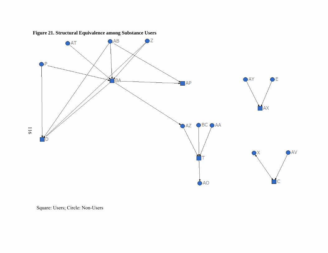
116
Figure 21. Structural Equivalence among Substance Users
Square: Users; Circle: Non-Users

117
Whereas actors D and AP who occupy structurally similar positions show similar levels
of substance use for both alcohol and marijuana, actors AX and BA occupy structurally
dissimilar positions and engage in very different levels of substance use. Taken together, these
findings provide evidence that allows us to conclude, at least tentatively, that substance users
with structurally similar, if not equivalent, positions are more likely to exhibit the similar levels
of substance use than will those who do not. Further, there may be more variation with regard
to the level of substance use among those who are in the less structurally equivalent positions.
Not only do actors who have structurally equivalent or similar positions exhibit similar
levels of substance use, but these structurally equivalent actors are also likely to be directly
connected to each other. This is similar to what Akers (2000: 83) refers to as “a bird joining a
flock and changing its feathers.” That is, one actor who associates with a substance user begins
use and then maintains a level of use similar to the other. However, as Akers admits (83)
differential association with substance users is often more likely to a consequence rather than a
cause. Thus, some might argue, as Hirschi (1969) no doubt would, that the findings here are
more an outcome of the process of social selection. That is, “birds of a feather flock together.”
Although this does not go beyond speculation due to the absence of friendship information in
Waves II and III, the results offer evidence of a selection effect.
Considering the presence of ties between substance users, co-offending is no doubt
likely to occur. However, although having similar positions may be necessary for co-offending,
it is not sufficient to explain it. Similarly, having ties between actors is essential to co-offend,
but again is not sufficient to explain it. Both conditions must exist simultaneously for co-
offending to occur. In this example, actors D and AP are in the roughly equivalent positions,
but the two not connected. Without a direct tie between D and AP, they are less likely to co-
118
offend. On the other hand, actors D and BA and AP and BA have relatively similar positions
and each pair is connected. In this case, each pair of actors has greater likelihood of co-
offending.
Examining Structural Equivalence allows us to understand that most of the group
members engage in substance use at similar level. Moreover, the connections among actors
imply the possibility of co-offending. Here I can only conclude that individuals who share
similar positions within a group tend to engage in similar levels of substance use.
Summary and Conclusion
The purpose of the case study is to enhance our understanding of substance use by
providing a visual representation of the findings in the quantitative study. In general, this case
study reflects the findings from the quantitative study. The correlation between network
characteristics and substance use puts substance users in center of relatively well defined
subgroups. Although there is no way to determine definitively whether these users co-offend
or offend individually, substance use and in particular marijuana use tends to take the form of
co-offending. In this sense, the results are at least consistent with the notion of co-offending
among substance users.
As discussed in the quantitative study, higher Centrality may reflect the tendency of
some youthful actors to “show-off” or engage in “groupie” type behavior. Without recognition
from others, it is perhaps questionable whether opportunities for substance use exist for fringe
members. On the other hand, Prestige directly reflects opportunities for substance use given
the nature of their connections to others. It is also possible that their experience with substance
use is the reason for their popularity, which in turn may provide additional opportunities for
substance use. Finally, not only do actors who have structurally equivalent or at least similar

119
positions exhibit similar levels of substance use, but also these actors are likely to be directly
connected to each other. This again suggests that the possibility of co-offending.
It is important to note that there are only a few substance users in the school chosen for
the case study. There are a few plausible reasons for this. First, given the nature of the
“saturated sample,” students who responded may be very conventional and thus willing to
participate in the lengthy in-home interview with less concern about the confidentiality of their
responses than would frequent users. In addition, as with any study using self-reported
behavior and attitudes, it is possible that their responses reflect expected rather than actual
behavior and attitudes. Second, this school includes students in grades 7 through 12 grades and
this may have limited the distribution of substance use given the inclusion of a large proportion
of younger students. This may also reflect a potential school size effect. For example, the
function of density can be applied to the school as a whole. In a small school, students are
more likely to know each other which may result in fewer substance users than in the general
adolescent population. Further, the racial/ethnic homogeneity of the school may contribute to a
small number of substance users and the relatively low level of substance use even among users.
Despite these caveats, it appears that overall the findings from the case study are generally
consistent with the results in the quantitative study.

120
CHAPTER SEVEN
SUMMARY AND CONCLUSION
Discussion
This study has focused on the structure of adolescent friendship networks and examined
how one’s position in these structures affects substance use. Using data from a national panel
study of in-school youth, I examined the effects of four network variables, Centrality, Prestige,
Density, and Heterogeneity on substance use during high school and then again when the
respondents were in their mid-twenties. It is clear from the findings that although the structure
of friendship networks impact substance use the effects vary by race/ethnicity, and substance
type, and time.
Contrary to expectations, my initial analysis revealed that the network variables showed
little overall effect on underage drinking. However, when interactions with race/ethnicity were
taken into account the effects of Centrality, Prestige, and Density were found to be statistically
significant although direction of the effects varied somewhat by group. For example, whereas
the overall effect of Density on alcohol use was negative, it had a significant positive effect on
alcohol use among both African American and Asian youth. Centrality showed a significant
positive effect only among African Americans. On the other hand, Prestige or popularity had a
significant positive effect regardless of racial/ethnic group while Heterogeneity was found to be
not significant even after race/ethnicity was taken into account. However, it is possible that the
small sample size may account lack of statistical significance for Native Americans.
The findings for marijuana use were somewhat different. Contrary to expectations,
Centrality was negatively associated with marijuana use. However, and consistent with the

121
findings for alcohol use, Prestige was positively associated with use. These results suggest that
within their friendship groups, marijuana users tended to be popular individuals who rarely
nominated others as friends. This combined with the finding that Heterogeneity was also
positively associated with marijuana would seem to suggest that these groups tend not to be
very cohesive. In fact, Density had no significant effect on marijuana use. The picture that
emerges is one in which marijuana users tend to be in the center of loosely organized groups.
This seems consistent with Orcutt’s (1978) observation that individuals engage in marijuana
use for personal rather than social reasons.
As with alcohol use when interactions with race/ethnicity were taken into account, all
network variables were significant and again the direction of these effects on marijuana use
again varied somewhat across groups. Density appeared to serve as a facilitating factor only
among African Americans and Hispanics. Consistent with alcohol use, Centrality had a
significant negative effect whereas Prestige had a significant positive effect regardless of
race/ethnicity. Unlike the findings for alcohol use, Heterogeneity appeared to have a strong
facilitating effect across all racial/ethnic groups.
What both alcohol and marijuana use have in common is that when the interaction terms
between race/ethnicity and network variables are incorporated, Centrality, Prestige, and
Density had significant effects for the sample as a whole although the importance of Centrality
and Density did vary by race/ethnicity. Apart from that the major difference is that
Heterogeneity appeared to have a strong facilitating effect across all racial/ethnic groups for
marijuana use but not for alcohol.
As expected the results revealed that attachment to parents is a strong constraining
factor with regard to both alcohol and marijuana use. When the attachment to parents is
122
controlled, the effects of the network variables became stronger. Because juveniles can be
attached both to parents and to peers, the principal influence here is not entirely clear.
However, the findings seem consistent with Warr’s (1993a) conclusion that attachment to
parents may discourage adolescents from developing initial friendships with delinquent peers,
but those ties are less constraining once exposure to delinquent youth occurs. In this study,
peer influence is measured in terms of structural proximity. The findings indicate that
adolescents are more likely to be affected by the friendship structure when attachment to
parents is held equal. This further indicates that adolescents who report strong attachment to
their parents are less likely to be involved in and therefore less influenced by their location in
peer group structures. This suggests that when parental control is strong youth are less likely to
select friends or be selected by others who are engaged in substance use. Given that, they
should be less affected by peer group socialization processes.
The most salient finding for short-term alcohol and marijuana use is the effect of
Prestige. Prestige shows a consistent positive effect on substance use regardless of
race/ethnicity. This is partially consistent with Kreager and Staff’s (2009) finding based on
Cohen’s (1955) theory of how subcultures are formed. According to Kreager and Staff, peer
acceptance level is associated with the number of sexual partners boys have and especially boys
from lower socioeconomic status backgrounds. Both findings suggest the possibility of a
reverse causal effect, that is, because of one’s past antisocial behavior an adolescent may be
popular among peers.
When I examined the effects of network variables on later substance use, the findings
with respect to alcohol use provide strong support for the hypothesis that adolescent friendship
networks will impact future use as people enter their mid-twenties. For alcohol, Centrality and
123
Prestige were found to be positively associated with future use while Density showed a
negative effect. This is also true for the measures of binge drinking and problem drinking at
Wave III. Interestingly, the findings for later marijuana use and other illegal/unauthorized drug
use are somewhat different. Here Heterogeneity in adolescent friendship groups is related to
only for the use of these substances when the respondents were in their mid-twenties.
Involvement in these more serious offenses appears to have less to do with one’s position in
early friendship groups than the type of groups in which they were involved. Nevertheless, the
findings suggest that the effect of early alcohol and marijuana use on later alcohol, marijuana,
and other illicit/unauthorized drug use is weakened, though only slightly, when adolescent
network variables are controlled.
The major difference between alcohol and marijuana use is that the short-term network
variables are more likely to be significant for marijuana use whereas the long-term network
effects are relatively greater for both substances. In addition, Density affects both short-term
and long-term alcohol use and Heterogeneity affects both short-term and long-term marijuana
use. It is interesting to examine these differences in light of Sutherland’s (1947) position that
exposure to definitions favorable to the violation of the law vary in terms of frequency,
duration, intensity and priority. These findings suggest that friendship networks established
during the adolescent years will affect later drinking behavior because the associations with
peers, and in this case those formed in school, are frequent and take on increasing importance
through the adolescent years. These effects are perhaps particularly important for those who at
some point begin using alcohol, which though illegal for youth, will eventually be “approved.”
In a sense, once peer groups are established this pattern is likely to continue over time.
Because alcohol is generally considered to be a socially approved substance one’s positions in

124
early friendship networks appear to be more important for later use. Marijuana use, on the
other hand, is less likely to receive the same level of social approval from others. That is, any
socialization to group expectations that occurred during early networks appears to carry over to
later marijuana use.
The above appears to be related to the general trajectories identified for these
substances. As adolescents reach legal age, drinking behavior is more likely to be approved;
thus alcohol use in general showed an upward trajectory. On the other hand, marijuana use is
illegal regardless of age; therefore, and consistent with Hirschi’s notion of commitment, as
individuals grow older and as they develop stakes in conformity, the trajectory for marijuana
shows a downward direction. These trajectory patterns are generally consistent with the
regression analyses.
As already noted, these data suggest that marijuana use is most likely to occur among
isolated individuals located in less cohesive groups. If Orcutt (1978) is correct these
individuals are likely engage in marijuana use over time for personal reasons. Individuals who
were in heterogeneous groups during high school appear to be less likely to nominate others as
friends. In heterogeneous groups, which are less cohesive, individuals may develop
predisposition such as “going one’s way” and the effect of Heterogeneity appeared to continue
over time. However, there is some evidence that this relationship differs by race/ethnic group.
For example, the effect of early drinking on later drinking and binge drinking was not found
among Native Americans. Also, early marijuana use was not associated with later
illicit/unauthorized drug use among African American and Native American youth.
Despite some limitations due to the composition of the school involved, the case study
findings were generally consistent with those in the quantitative analyses. Centrality or active
125
nominations is not related to substance use whereas users are likely to have greater Prestige
among their peers. Furthermore, the Density measure for users was lower than average, which
is also consistent with findings from the quantitative analysis. Although the prevalence of
substance use among the case study sample was very low, the results nevertheless revealed at
least one unique function of network variables that was not apparent in the quantitative analysis.
That is, substance users who shared structurally similar positions had similar levels of
substance use whereas users who held dissimilar positions showed different levels of use.
Identifying individuals who are in the similar positions in groups, particularly within school,
may be useful for intervention strategies designed to assist substance uses.
As noted throughout, past research has rarely paid attention to structural proximity
within friendship groups as this relates to substance use and perhaps delinquent behavior in
general. Warr and Stafford (1991) report that one’s delinquency involvement is not just the
result of friends’ attitudes; rather, other social learning concepts such as imitation may also
influence one’s behavior. Structural proximity would seem to be essential for an actor to
observe and then imitate others’ antisocial behavior. However, the findings from this study
revealed that for the most part the effects of network variables on alcohol and marijuana use do
not overlap in either the short-term or the long-term despite the strong correlation between the
two. This may be explained by the fact marijuana users are more likely to use alcohol while
alcohol users are not necessarily marijuana users. The data showed that 67 percent of
marijuana users used alcohol as well whereas only 45 percent of alcohol users used marijuana
concurrently. It would seem then, that there may be important differences between alcohol and
marijuana use due to different legal definitions and general notions of acceptability. In addition,
126
and consistent with Orcutt’s (1978) findings, the motivation for alcohol use tends to be social
whereas the motivation for marijuana is likely to be personal.
Network analysis should help explain both the process of social selection as well as
socialization based on structural proximity. Although both Centrality and Prestige identify
one’s position in a group, the effect of Centrality on behavior was not found to be as consistent
as the effect of Prestige. While Prestige always indicates that an individual is the center of
attention, Centrality does not. This may mean, of course, that Prestige is a better measure of
one’s location in a group. Whether or not that is the case it does appear, as Reckless (1961)
argued, that Prestige serves as a “push” factor. Heterogeneity, it would seem, is also likely to
function as a facilitating or “push” factor in the sense that it is associated with a lack of
cohesion or Density within groups and therefore a lack of conventional social controls (see for
example, Shaw and McKay 1942). On the other hand, Density appears to serve as a
constraining or “pull” factor.
Limitations
Several limitations of the present study need to be addressed. First, as with most studies
of delinquency and substance use, the distributions of these behaviors are highly skewed. As
with studies of delinquency involvement (see Haynie 2001), the distributions of the dependent
variables are highly skewed. This is particularly true for in-school self-report surveys because
many serious delinquents and substance users have dropped out of school (Cernkovich et al.
1985). In this study, adolescents who participated in both the in-school survey and the at-home
interviews at all three waves are perhaps even more unlikely to have engaged in or to report
serious and excessive substance use.
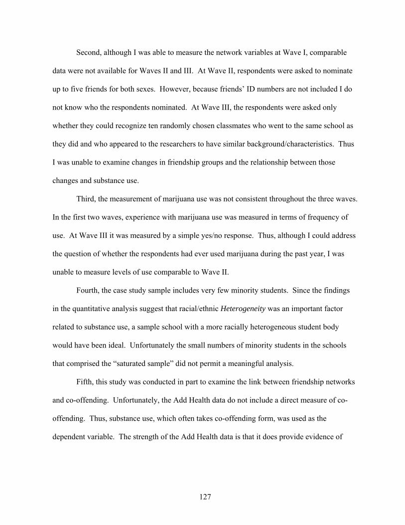
127
Second, although I was able to measure the network variables at Wave I, comparable
data were not available for Waves II and III. At Wave II, respondents were asked to nominate
up to five friends for both sexes. However, because friends’ ID numbers are not included I do
not know who the respondents nominated. At Wave III, the respondents were asked only
whether they could recognize ten randomly chosen classmates who went to the same school as
they did and who appeared to the researchers to have similar background/characteristics. Thus
I was unable to examine changes in friendship groups and the relationship between those
changes and substance use.
Third, the measurement of marijuana use was not consistent throughout the three waves.
In the first two waves, experience with marijuana use was measured in terms of frequency of
use. At Wave III it was measured by a simple yes/no response. Thus, although I could address
the question of whether the respondents had ever used marijuana during the past year, I was
unable to measure levels of use comparable to Wave II.
Fourth, the case study sample includes very few minority students. Since the findings
in the quantitative analysis suggest that racial/ethnic Heterogeneity was an important factor
related to substance use, a sample school with a more racially heterogeneous student body
would have been ideal. Unfortunately the small numbers of minority students in the schools
that comprised the “saturated sample” did not permit a meaningful analysis.
Fifth, this study was conducted in part to examine the link between friendship networks
and co-offending. Unfortunately, the Add Health data do not include a direct measure of co-
offending. Thus, substance use, which often takes co-offending form, was used as the
dependent variable. The strength of the Add Health data is that it does provide evidence of
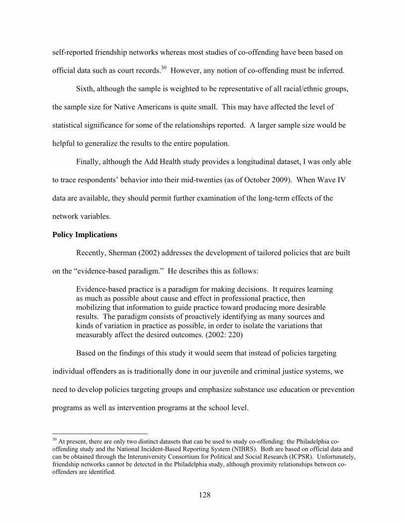
128
self-reported friendship networks whereas most studies of co-offending have been based on
official data such as court records.30 However, any notion of co-offending must be inferred.
Sixth, although the sample is weighted to be representative of all racial/ethnic groups,
the sample size for Native Americans is quite small. This may have affected the level of
statistical significance for some of the relationships reported. A larger sample size would be
helpful to generalize the results to the entire population.
Finally, although the Add Health study provides a longitudinal dataset, I was only able
to trace respondents’ behavior into their mid-twenties (as of October 2009). When Wave IV
data are available, they should permit further examination of the long-term effects of the
network variables.
Policy Implications
Recently, Sherman (2002) addresses the development of tailored policies that are built
on the “evidence-based paradigm.” He describes this as follows:
Evidence-based practice is a paradigm for making decisions. It requires learning as much as possible about cause and effect in professional practice, then mobilizing that information to guide practice toward producing more desirable results. The paradigm consists of proactively identifying as many sources and kinds of variation in practice as possible, in order to isolate the variations that measurably affect the desired outcomes. (2002: 220) Based on the findings of this study it would seem that instead of policies targeting
individual offenders as is traditionally done in our juvenile and criminal justice systems, we
need to develop policies targeting groups and emphasize substance use education or prevention
programs as well as intervention programs at the school level.
30 At present, there are only two distinct datasets that can be used to study co-offending: the Philadelphia co-offending study and the National Incident-Based Reporting System (NIBRS). Both are based on official data and can be obtained through the Interuniversity Consortium for Political and Social Research (ICPSR). Unfortunately, friendship networks cannot be detected in the Philadelphia study, although proximity relationships between co-offenders are identified.
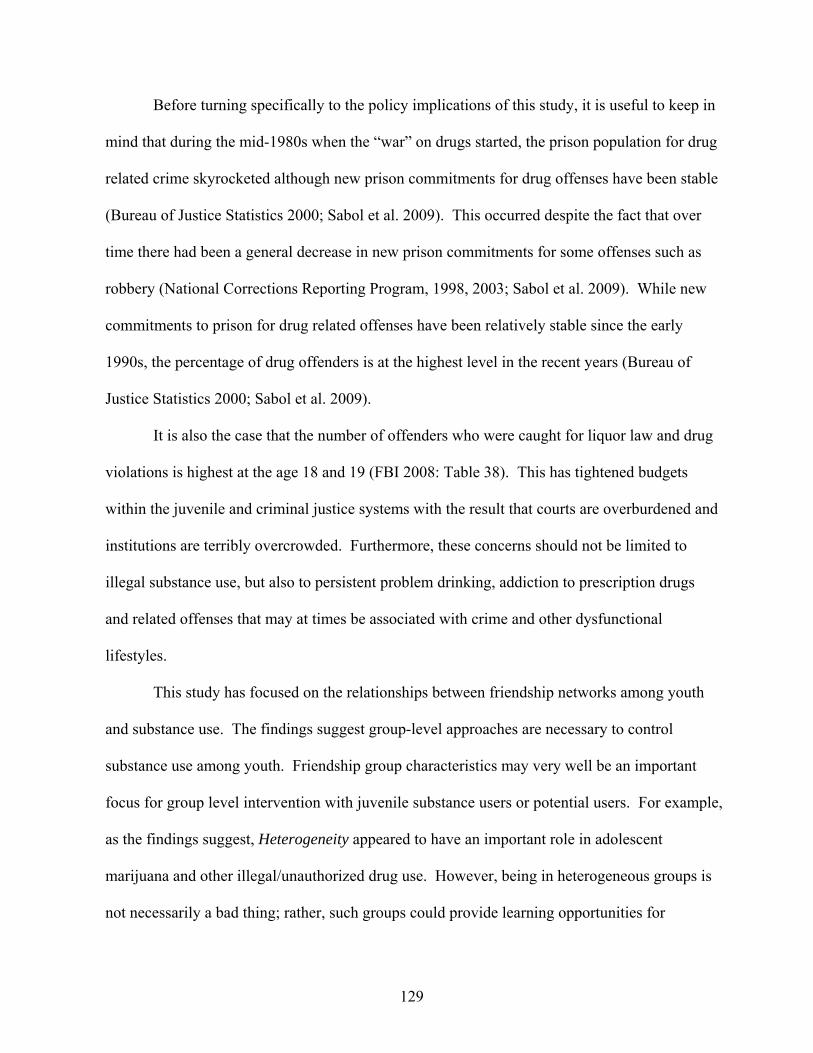
129
Before turning specifically to the policy implications of this study, it is useful to keep in
mind that during the mid-1980s when the “war” on drugs started, the prison population for drug
related crime skyrocketed although new prison commitments for drug offenses have been stable
(Bureau of Justice Statistics 2000; Sabol et al. 2009). This occurred despite the fact that over
time there had been a general decrease in new prison commitments for some offenses such as
robbery (National Corrections Reporting Program, 1998, 2003; Sabol et al. 2009). While new
commitments to prison for drug related offenses have been relatively stable since the early
1990s, the percentage of drug offenders is at the highest level in the recent years (Bureau of
Justice Statistics 2000; Sabol et al. 2009).
It is also the case that the number of offenders who were caught for liquor law and drug
violations is highest at the age 18 and 19 (FBI 2008: Table 38). This has tightened budgets
within the juvenile and criminal justice systems with the result that courts are overburdened and
institutions are terribly overcrowded. Furthermore, these concerns should not be limited to
illegal substance use, but also to persistent problem drinking, addiction to prescription drugs
and related offenses that may at times be associated with crime and other dysfunctional
lifestyles.
This study has focused on the relationships between friendship networks among youth
and substance use. The findings suggest group-level approaches are necessary to control
substance use among youth. Friendship group characteristics may very well be an important
focus for group level intervention with juvenile substance users or potential users. For example,
as the findings suggest, Heterogeneity appeared to have an important role in adolescent
marijuana and other illegal/unauthorized drug use. However, being in heterogeneous groups is
not necessarily a bad thing; rather, such groups could provide learning opportunities for

130
adolescents by exposure to diverse culture. An understanding of differences may promote
adolescent prudence, interest in others, and maturity. Thus, we have to find ways to integrate
those involved in heterogeneous groups into mainstream activities. Efforts to involve
adolescents in homogeneous groups in terms of common interests and goals and that maintain
conventional values/norms would seem to be a productive approach to temper current and
future use if this approach creates a sense of belonging among adolescents. Along with
common interests and goals, race/ethnicity may be particularly important because network
characteristics appear to function uniquely in some racial/ethnic groups. Whatever the
approach, it does seem clear that some form of intervention is necessary to be effective for
certain groups. However, we should consider that different approaches for alcohol and other
illegal drug use are necessary given the different legal definitions involved.
McCurley and Snyder (2008) report that 32 percent of alcohol users also used marijuana
and 81 percent of marijuana users also report alcohol use. The percentage of co-occurrence of
substance use in this study is, as noted earlier, slightly different from this report (45 percent of
alcohol users engaged in marijuana use while 67 percent of marijuana users also engaged in
alcohol use). However, this is close enough to suggest that co-occurrence of substance use
among youth is likely, and leads some legitimacy to concluding that early discovery of
substance problems and intervention at a group level may work by targeting high-risk
offending groups that include concurrent and higher level substance users at the school level if
this can be accomplished by not stigmatizing those involved.
Some suggest that legal/political interventions that crack down on juvenile offenses
committed by co-offenders will decrease the likelihood of substance use among adolescents.
However, based on the results of this research, cracking down on marijuana use is probably not
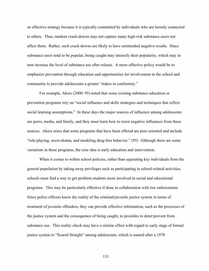
131
an effective strategy because it is typically committed by individuals who are loosely connected
to others. Thus, random crack-downs may not capture many high-risk substance users nor
affect them. Rather, such crack-downs are likely to have unintended negative results. Since
substance users tend to be popular, being caught may intensify their popularity, which may in
turn increase the level of substance use after release. A more effective policy would be to
emphasize prevention through education and opportunities for involvement in the school and
community to provide adolescents a greater “stakes in conformity.”
For example, Akers (2000: 95) noted that some existing substance education or
prevention programs rely on “social influence and skills strategies and techniques that reflect
social learning assumptions.” In these days the major sources of influence among adolescents
are peers, media, and family, and they must learn how to resist negative influences from these
sources. Akers notes that some programs that have been offered are peer-oriented and include
“role-playing, socio-drama, and modeling drug-free behavior.” (95) Although there are some
variations in these programs, the core idea is early education and intervention.
When it comes to within school policies, rather than separating key individuals from the
general population by taking away privileges such as participating in school-related activities,
schools must find a way to get problem students more involved in social and educational
programs. This may be particularly effective if done in collaboration with law enforcement.
Since police officers know the reality of the criminal/juvenile justice system in terms of
treatment of juvenile offenders, they can provide effective information, such as the processes of
the justice system and the consequence of being caught, to juveniles to deter/prevent from
substance use. This reality check may have a similar effect with regard to early stage of formal
justice system to “Scared Straight” among adolescents, which is named after a 1978
132
documentary film (Akers 2000). Although we must keep in mind that many youth are not
seriously involved in school activities, school administrators may nevertheless create appealing
extracurricular activities and/or give positive incentives or rewards to increase their stakes in
conformity. I believe that education rather than formal sanctions will be more effective and
give adolescents a second chance for their future without stigmatizing them.
Lastly, identifying structurally equivalent or similar individuals within groups is
important for early intervention. The case study revealed that substance users share similar
positions. Once one substance user is identified, schools can provide early intervention with a
group of youth by creating structural dissimilarity in a group by increasing the level of
closeness between members or by introducing new non-delinquent members to the group to
instill some positive effects.
Conclusion
As Sarnecki (2001: 168) notes, network analysis is “a theoretically neutral
methodological tool” that appears to be particularly appropriate for studies of substance use.
Network characteristics not only indicate how actors think about their relationships with others
but also how others think about them. Unfortunately, although network scholars share core
concepts, there is little agreement on definitions, specific features of social networks, and
terminology (Fischer 1977, 33). With that in mind, researchers are required to provide their
own definitions of terms and features before moving into analyses. They must specify the
scope of the research, and what they want to measure and analyze. In order for network
analyses to be used widely in the discipline of criminology/delinquency, scholars must work
together to clarify their terminology and concepts.

133
The effect of social selection and socialization effects should be understood in the
context of group dynamics rather than differences in personal characteristics. Peers or
friendship groups are a major part of adolescent life as they grow older. The findings in this
study suggest that much of what goes on during the adolescent years impacts both current and
future behavior.
134
BIBLIOGRAPHY Adler, Patricia A. and Peter Adler. 1983. ‘Shifts and Oscillations in Deviant Careers: The Case
of Upper-Level Drug Dealers and Smugglers.” Social Problems 31 (2): 195-207. Agnew, Robert. 2009. Juvenile Delinquency: Causes and Control (third edition). Roxbury
Publishing Company: CA Akaike, H. 1974. “A New Look at the Statistical Identification Model,” IEEE Trans. Auto Control 19: 716-723. Akers, Ronald L. 2000. (third edition) Criminological Theories: Introduction, Evaluation, and Application. Roxbury Publishing Company: CA Akers, Ronald L. 1998. Social learning and Social Structure: A General Theory of Crime and
deviance. Northeastern University Press: MA Akers, Ronald L. 1992. Drugs, Alcohol, and Society: Social Structure, Process, and Policy.
Wadsworth Publishing Company: CA Akers, Ronald L. 1992. “Linking Sociology and its Specialties: The Case of Criminology.”
Social Forces 71: 1-16. Akers, Ronald L., Marvin D. Krohn, Lonn Lanza-Kaduce, and Marcia Radosevich. 1979.
“Social Learning and Deviant Behavior: A Specific Test of a General Theory.” American Sociological Review 44: 636-655.
Akers, Ronald L. and Gang Lee. 1999. “Age, Social Learning, and Social Bonding in
Adolescent Substance Use.” Deviant Behavior 19: 1-25. Akers, Ronald L. and Gang Lee. 1996. “A Longitudinal Test of Social Learning Theory:
Adolescent Smoking.” Journal of Drug Issues 26:317-343. Baerveldt, Chris and Tom Snijders. 1994. “Influences on and from the Segmentation of
Networks: Hypotheses and Tests.” Social Networks 16 (3): 213-232. Barnes, Grace M., John W. Welte, and Barbara Dintcheff. 1992. “Alcohol Misuse Among
College Students and Other Young Adults: Findings from a General Population Study in New York state.” International Journal of the Addictions 27 (8): 917-934.
Bayes, Thomas. 1763. “An essay towards solving a problem in the doctrine of chances.”
Philosophical Transactions 53: 370-418. Borgatti, S.P., M.G. Everett, and L.C. Freeman. 2002. UCINET for Windows: Software for
Social Network Analysis http://www.analytictech.com. Analytic Technologies: MA
135
Bureau of Justice Statistics. 2003. “National Corrections Reporting Program, 2003.” U.S. Department of Justice, Office of Justice Programs: DC
Bureau of Justice Statistics. 2000. “Correctional Populations in the United States, 1997.” U.S.
Department of Justice, Office of Justice Programs: DC Bureau of Justice Statistics. 1998. “National Corrections Reporting Program, 1998.” U.S.
Department of Justice, Office of Justice Programs: DC Burkett, Steven R. 1993. “Perceived Parents’ Religiosity, Friends’ Drinking, and Hellfire: A
Panel Study of Adolescent Drinking.” Review of Religious Research 35 (2): 134-154. Burkett, Steven R. 1977a. “Religion, Parental Influence, and Adolescent Alcohol and
Marijuana Use.” Journal of Drug Issues 7 (3): 263-273. Burkett, Steven R. 1977b. “School Ties, Peer Influence and Adolescent Marijuaana Use.”
Pacific Sociological Review 20: 181-195. Burkett, Steven R. and Eric L. Jensen. 1975. “Conventional Ties, Peer Influence and Fear of
Apprehension: A Study of Adolescent Marijuana Use.” Sociological Quarterly 16: 522-533.
Burt, Ronald S. 1978. “Cohesion versus Structural Equivalence as a Basis for Network
Subgroups.” Sociological Methods and Research 7 (2): 189-212. Burt, Ronald S. 1976. “Position in Networks.” Social Forces 55 (1): 93-122. Cairns, Robert B. and Beverly D. Cairns. 1994. Lifelines and Risks: Pathways of Youth in Our
Time. Cambridge University Press: NY or UK Catalano, Richard and J. David Hawkins. 1996. “The social development model: a theory of
antisocial behavior,” Pp. 149-197 In Delinquency and Crime: Current Theories, edited by J. David Hawkins, Cambridge University Press: NY
Cernkovich, Stephen, Peggy Giordano, and Meredith Pugh. 1985. “Chronic Offenders: The
Missing Cases in Self-Report Delinquency Research.” Journal of Criminal Law and Criminology 76 (3): 705-732.
Cohen, Albert, K. 1955. Delinquent Boys. Free Press: IL Coleman, James S. 1961. The Adolescent Society: The Social Life of the Teenager and its
Impact on Education. The Free Press of Glencoe: NY Duncan, Terry E., Susan C. Duncan, and Lisa A. Strycker. 2006. An Introduction to Latent
Variable Growth Curve Modeling: Concepts, Issues, and Applications. (Second Edition) Lawrence Erlbaum Associates, Inc.: NJ
136
D’Unger, Amy V., Kenneth C. Land, Patricia L. McCall, and Daniel S. Nagin. 1998. “How Many Latent Classes of Delinquent/Criminal Careers? American Journal of Sociology 103 (6): 1593-1630.
Elliott, Delbert and Harwin Voss. 1974. Delinquency and Dropout. D.C. Health: MA Erickson, Maynard L. 1973. “Group Violations, Socioeconomic Status and Official
Delinquency.” Social Forces 52(1): 41-52. Erickson, Maynard L. 1971. “The Group Context of Delinquent Behavior.” Social Problems
19: 114-129. Erickson, Maynard L. and Gary F. Jensesn. 1977. “Delinquency Is Still Group Behavior!:
Toward Revitalizing the Group Premise in the Sociology of Deviance.” Journal of Criminal Law and Criminology 68: 262-273.
Federal Bureau of Investigation. 2008. “Crimes in the United States Table 38”
http://www.fbi.gov/ucr/cius2008/data/table_38.html Farrington, David P. 1986. “Age and Crime,” Pp. 189-250. In Crime and Justice: An Annual
Review of Research, Vol. 7, edited by Michael Tonry and Norval Morris, The University of Chicago Press: IL
Finn, Kristin V. 2006. “Patterns of Alcohol and Marijuana Use at School.” Journal of Research
on Adolescence 16 (1): 69-77. Fischer, Claude S. 1977. “Network Analysis and Urban Studies.” Networks and Places: Social
Relations in the Urban Setting. The Free Press: NY Fleisher, Mark S. 2002. “Doing Field Research on Diverse Gangs: Interpreting Youth Gangs as Social Networks.” In Gangs in America III, edited by C. Ronald Huff, Sage
Publications: CA Fleisher, Mark S. 2000. Dead End Kids: Gang Girls and the Boys They Know. The University
of Wisconsin Press: WI Friday, Paul C. and Jerald Hage. 1976. “Youth Crime in Postindustriaal Societies: An
Integrated Perspective.” Criminology 14: 347-68. Garnier, Helen E. and Judith A. Stein. 2002. “An 18-Year Model of Family and Peer Effects on
Adolescent Drug Use and Delinquency,” Journal of Youth and Adolescence 31 (1): 45-56.
Glueck, Sheldon and Eleanor Glueck. 1950. Unraveling Juvenile Delinquency. Commonwealth
Fund: New York

137
Gottfredson, Michael R. and Travis Hirschi. 1990. A General Theory of Crime. Stanford University Press: CA
Hamilton, Lawrence C. 2003. Statistics with STATA 7. Duxbury Press: CA Hamilton, Lawrence C. 1992. Regression with Graphics: A Second Course in Applied Statistics.
Duxbury Press: CA Harris, K.M., C.T. Halpern, E. Whitsel, J. Hussey, J. Tabor, P. Entzel, and J.R. Udry. 2009.
The National Longitudinal Study of Adolescent Health: Research Design [WWW document]. URL: http://www.cpc.unc.edu/projects/addhealth/design.
Harris, Kathleen Mullan, and J. Richard Udry. National Longitudinal Study of Adolescent
Health (Add Health), 1994-2002 [Computer file]. ICPSR21600-v2. Ann Arbor, MI: Inter-university Consortium for Political and Social Research [distributor], 2008-10-31. doi:10.3886/ICPSR21600.
Hawkins, J. David and Joseph G. Weis. 1985. “The social development model: an integrated
approach to delinquency prevention.” Journal of Primary Prevention 6:73-97. Haynie, Dana L. 2002. “Friendship Networks and Delinquency: The Relative Nature of Peer
Delinquency.” Journal of Quantitative Criminology 18 (2): 99-134. Haynie, Dana L. 2001. “Delinquent Peers Revisited: Does Network Structure Matter?”
American Journal of Sociology 106 (4): 1013-1057. Haynie. Dana L. and D.Wayne Osgood. 2005. “Reconsidering Peers and Delinquency: How Do
Peers Matter?” Social Forces 84 (2): 1109-1130. Hays, R.B. 1988. “Friendship,” in Handbook of Personal relationships: Theory, Research, and
Interventions, edited by S.W. Duck, Wiley: NY Hirschi, Travis. 1969. Causes of Delinquency. University of California Press: CA Horney, Julie, D. Wayne Osgood, and Ineke Haen Marshall. 1995. “Criminal Careers in the
Short-term: Intra-individual Variability in Crime and Its Relation to Local Life Circumstances.” American Sociological Review 60 (5): 655-673.
Jensen, Gary F. 1972. “Parents, Peers, and Delinquent Action: A Test of the Differential
Association Perspective.” American Journal of Sociology 78: 562-575. Johnston, L. D., P. M. O’Malley, J. G. Bachman, and J. E. Schulenberg. 2007. “Monitoring the
Future National Results on Adolescent Drug Use: Overview of Key Findings, 2006 (NIH Publication Number 07-6202).” National Institute on Drug Abuse: MD
138
Kashyap, R. 1980. “Inconsistency of the AIC Rule for Estimating the Order of Autoregressive Models.” IEEE Tans. Auto Control 25 (5): 996-998.
Kim-Cohen, Julia Terrie E. Moffitt, Avshalom Caspi, and Alan Taylor. 2004. “Genetic and
Environmental Processes in Young Children’s Resilience and Vulnerability to Socioeconomic Deprivation.” Child Development 75 (3): 651-668.
Klein, Malcolm W. 1995. The American Street Gang: Its Nature, Prevalence, and Control.
Oxford University Press: NY Klein, Malcolm W. 1971. Street Gangs and Street Workers. Prentice Hall: NJ Kreager, Derek A. and Jeremy Staff. 2009. “The Sexual Double Standard and Adolescent Peer
Acceptance.” Social Psychology Quarterly 72 (2): 143-164. Krohn, Marvin D. 1986. “The web of conformity: A network approach to the explanation of delinquent behavior.” Social problems 33: S81—S93. Krohn, Marvin D., Ronald L. Akers, Marcia J. Radosevich, and Lonn Lanza-Kaduce. 1982.
“Norm Qualities and Adolescent Drinking and Drug Behavior.” Journal of Drug Issues 12: 343-359.
Krohn, Marvin D., Lonn Lanza-Kaduce, and Ronald L. Akers. 1984. “Community Context and
Theories of Deviant Behavior: An Examination of Social Learning and Social Bonding Theories.” Sociological Quarterly 25: 353-371.
Krohn, Marvin D. and James L. Massey. 1980. “Social Control and Delinquent Behavior: An
Examination of the Elements of the Social Bond.” The Sociological Quarterly 21 (4): 529-543.
Krohn, Marvin D., James L. Massey, and Mary Zielinski. 1988. “Role Overlap, Network
multiplexity, and Adolescent Deviant behavior.” Social Psychology Quarterly 51 (4): 346-356.
Krohn, Marvin D. and Terence P. Thornberry. 1993. “Network Theory: A Model for
Understanding Drug Abuse Among African-American and Hispanic Youth.” In Drug Abuse Among Minority Youth: Advances in Research and Methodology (NIDA Research Monograph 130), edited by Mario R. De La Rosa and Juan-Luis Recio Adrados, National Institute on Drug Abuse: MD
Laub, John H. and Robert J. Sampson. 1993. “Turning points in the life course: why change
matters to the study of crime.” Criminology 31: 301-326. Lee, Gang, Ronald L. Akers, and Marian J. Borg. 2004. “Social Learning and Structural
Factors in Adolescent Substance Use.” Western Criminology Review 5 (1): 17-34.

139
Liska, Allen E. 1978. “Deviant Involvement, Associations and Attitudes: Specifying the Underlying Causal Structures.” Sociology and Social Research 63: 73-88.
Liska, Allen E. and Steven F. Messner. 1999. Perspectives on Crime and Deviance. Prentice
Hall: NJ Le Blanc, Marc and Aaron Caplan. 1993. “Theoretical Formalization, a Necessity: The
Example of Hirschi’s Bonding Theory.” In Freda Adler and William S. Laufer, ed., New Directions is Criminological Theory Transaction Publishers: NJ
Loeber, Rolf. 1996. “Developmental continuity, change, and pathways in male juvenile
problem behaviors and delinquency.” Pp.1-27 in Delinquency and Crime: Current Theories, edited by J. David Hawkins, Cambridge University Press: NY
Loeber, Rolf, David P. Farrington, Magda Stouthamer-Loeber, Terrie Moffitt, and Avshalom
Caspi. 1998. “The development of male offending: key findings from the first decade of the Pittsburgh Youth Study.” Studies on Crime and Crime Prevention 7: 141-172.
Loeber, Rolf and M. LeBlanc. 1990. “Toward a developmental criminology,” Pp. 375-475 in
Crime and Justice: A Review of Research Vol.12. edited by Michael Tonry and Norvel Morris, University of Chicago Press: IL
Loeber, Rolf, Phen Wung, Kate Keenan, Bruce Giroux, Magda Stouthamer-Loeber, Wemoet
Van Kammen, and Barbara Maughan. 1993. “Developmental Pathways in Disruptive Behavior.” Development and Psychopathology 23: 12-48.
Lorrain, François and Harrison C. White. 1971. “Structural Equivalence of Individuals in
Social Networks.” Journal of Mathematical Sociology 1: 49-80. Maggs, Jennifer L. and Klaus Hurrelmann. 1998. “Do Substance Use and Delinquency Have
Differential Association with Adolescents’ Peer Relations?” International Journal of Behavioral Development 22 (2): 367-388.
Matza, David. 1964. Delinquency and Drift. John Wiley and Sons: NY McAdams, D. P. 1988. “Personal Needs and Personal Relationships,” In Handbook of Personal
relationships: Theory, Research, and Interventions. Edited by S.W.Duck, Wiley: NY McCord, Joan and Kevin P. Conway. 2002. “Patterns of Juvenile Delinquency and Co-
Offending.” In Crime and Social Organization edited by Elin Waring and David Weisburd, Transaction Publishers: NJ
McCurley, Carl and Howard N. Snyder. 2008. “Co-occurrence of Substance Use Behaviors in
Youth.” U.S .Department of Justice: Office of Justice Programs, and Office of Juvenile Justice and Delinquency Prevention. http://www.ncjrs.gov/pdffiles1/ojjdp/219239.pdf
140
Moffitt, Terrie E. 1993. “Adolescence-limited and life-course-persistent antisocial behavioral: a developmental taxonomy.” Psychological Review 100: 674-701.
Morash, M. 1983. “Gangs, Groups, and Delinquency.” British Journal of Criminology 23: 309-
331. Muthen, L. K. and B. O. Muthen. 2001. Mplus User’s Guide ***CA Nagin, Daniel S., David P. Farrington, and Terrie E. Moffitt. 1995. “Life-Course Trajectories
of Different Types of Offenders.” Criminology 33 (1): 111-139. Office of Juvenile Justice and Delinquency Prevention. 2008. “Juvenile Court Statistics 2005,”
http://www.ncjjservehttp.org/NCJJWebsite/pdf/jcsreports/jcs2005.pdf Orcutt, James D. 1978. “Deviance as a Situated Phenomenon: Variations in the Social
Interpretation of Marijuana and Alcohol Use.” Social Problems 22: 346-356. Polk, Kenneth and Walter E. Schafer. 1972. Schools and Delinquency. Prentice Hall: NJ Reckless, Walter C. 1961. “A New Theory of Crime and Delinquency.” Federal Probation 25:
42-46. Reiss, Albert J. Jr. 1988. “Co-Offending and Criminal Careers,” Pp. 117-170 in Crime and
Justice: A Review of Research (Volume 10), edited by Michael Tonry and Norval Morris, University of Chicago Press: IL Sabol, William J., Heather C. West, and Matthew Cooper. 2009. “Bureau of Justice Statistics
Bulletin, Prisoners in 2008.” U.S. Department of Justice, Office of Justice Programs: Washington DC
Sampson, Robert J. and John H. Laub. 2003. “Desistance from Crime over the Life Course,” pp.
295-309 in Handbook of the Life Course. Edited by Jeylan T. Mortimer and Michael J. Shanahan, Kluwer Academic/Plenum Publishers: NY
Sampson, Robert J. and John H. Laub. 1993. Crime in the Making: Pathways and Turning
Points Through Life. Harvard University Press: MA Sarnecki, Jerzy. 2001. Delinquent Networks: Youth Co-Offending in Stockholm. Cambridge University Press: UK Sarnecki, Jerzy. 1986. Delinquent Networks. The National Council for Crime Prevention: Sweden Schroeder, Ryan D., Peggy C. Giordano, and Stephen A. Cernkovich. 2007. “Drug Use and
Desistance Processes.” Criminology 45 (1): 191-222.

141
Schulenberg, John E., Alicia C. Merline, Lloyd D. Johnston, Patrick M. O’Malley, Jerald G. Bachman, and Virginia B. Laetz. 2005. “Trajectories of Marijuana Use During the Transition to Adulthood: The Big Picture Based on National Panel Data.” The Journal of Drug Issues 35 (2): 255-279.
Schwartz, Gideon. 1978. “Estimating the Dimension of a Model.” The Annals of Statistics 6
(2): 461-464. Scott, John. 1991. Social Network Analysis: A Handbook. Sage Publications: CA Shaw, Clifford R. 1966. The Jack-Roller: A Delinquent Boy’s Own Story. The University of
Chicago Press: IL Shaw, Clifford R. and Henry D. McKay. 1942. Juvenile Delinquency and Urban Areas.
University of Chicago Press: IL Shaw, Clifford R. and henry D. McKay. 1931. Report on the Causes of Crime, Volume II. U.S.
Government Printing Office: Washington D.C. Sherman, Lawrence W. 2002. “Evidence-Based Policing: Social Organization of Information
for Social Control.” In Elin Waring and David Weisburd eds., Crime and Social Organization, Transaction Publishers: NJ
Sutherland, Edwin H. 1947. Principles of Criminology, 4th Edition. J.P.Lippincolt: PA Thornberry, Terence P., Alan J. Lizotte, Marvin D. Krohn, Carolyn A. Smith, and Pamela K.
Porter. 2003. “Causes and Consequences of Delinquency: Findings from the Rochester Youth Development Study.” Pp. 11-46 in Taking Stock of Delinquency: An Overview of Findings from Contemporary Longitudinal Studies, edited by Terence P. Thornberry and Marvin D. Krohn, Plenum Publishers: NY
Thornberry, Terence P., Alan J. Lizotte, Marvin D. Krohn, Margaret Farnworth, and Sung Joon
Jang. 1994. “Delinquent Peers, Beliefs, and Delinquent Behavior: A Longitudinal Test of Interactional Theory.” Criminology 32 (1): 47-83.
Thornberry, Terence P., Marvin D. Krohn, Alan J. Lizotte, and Deborah Chard-Wierschem.
1993. “The Role of juvenile Gangs in Facilitating Delinquent Behavior.” Journal of Research in Crime and Delinquency, 30 (1): 55-87.
Thrasher, Frederic M. 1927. The Gang. The University of Chicago Press: IL UCLA Academic Technology Services. STATA Web Books: Regression with Stata.
http://www.ats.ucla.edu/stat/stata/webbooks/reg/chapter2/statareg2.htm U.S. Census Bureau. 2000. http://www.census.gov/prod/2002pubs/c2kprof00-us.pdf
142
U.S. Department of Health and Human Services: Substance Abuse and Mental Health Services Administration, Office of Applied Studies. 2004 (March). “How Youths Obtain Marijuana,” The NSDUH Report http://www.oas.samhsa.gov/2k4/MJsource/MJsource.pdf
Wagenaar, Alexander C., John R. Finnegan, Mark Wolfson, Pamela S. Anstine, Carolyn L.
Williams, Cheryl L. Perry. 1993. “Where and How Adolescents Obtain Alcoholic Beverages.” Public Health Reports 108(4):459-464.
Warr, Mark. 2002. Companions in Crime: The Social Aspects of Criminal Conduct. Cambridge University Press: NY
Warr, Mark. 1998. “Life-course transitions and desistance from crime.” Criminology 36 (2):
183-216. Warr, Mark. 1996. “Organization and Instigation in Delinquent Group.” Criminology 34 (1):
11-37. Warr, Mark. 1993a. “Parents, Peers, and Delinquency.” Social Forces 72 (1): 247-264. Warr, Mark. 1993b. “Age, Peers, and Delinquency.” Criminology 31: 17-40. Warr, Mark and Mark Stafford. 1991. “The Influence of Delinquent Peers: What they think or what they do?” Criminology 29 (4): 851-866. Wasserman, Stanley and Katherine Faust. 1994. Social Network Analysis. Cambridge
University Press: Cambridge, UK Weerman, Frank M. 2003. “Co-Offending as Social Exchange: Explaining Characteristics of
Co-Offending.” British Journal of Criminology 43 (2): 398-416. Wiesner, Margit and Michael Windle. 2004. “Assessing Covariates of Adolescent Delinquency
Trajectories: A Latent Growth Mixture Modeling Approach.” Journal of Youth and Adolescence 33 (5): 431-442.
Willmott, Peter. 1986. Social Networks, informal care and public policy. Policy Studies
Institute: UK Wright, John Paul and Francis T. Cullen. 2004. “Employment, Peers, and Life-course
Transitions.” Justice Quarterly 21 (1): 183-205. Yablonsky, Lewis. 1973. The Violent Gang. Penguin Books, Inc.: MD Yablonsky, Lewis. 1959. “The Delinquent Gang as a Near-Group.” Social Problems 7 (2): 108-
117. Zhang, Lening and Steven F. Messner. 2000. “The effects of alternative measures of delinquent

143
peers on self-reported delinquency.” Journal of Research in Crime & Delinquency. 7(3): 323-337.
Zeggelink, Evelien. 1993. Strangers into Friends: The Evolution of Friendship networks Using
an Individual Oriented Modeling Approach. Thesis Publishers: Netherlands
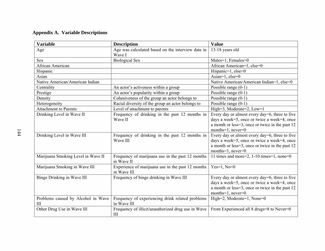
144
Appendix A. Variable Descriptions
Variable Description Value Age Age was calculated based on the interview date in
Wave I 13-18 years old
Sex Biological Sex Males=1, Females=0 African American African American=1, else=0 Hispanic Hispanic=1, else=0 Asian Asian=1, else=0 Native American/American Indian Native American/American Indian=1, else=0 Centrality An actor’s activeness within a group Possible range (0-1) Prestige An actor’s popularity within a group Possible range (0-1) Density Cohesiveness of the group an actor belongs to Possible range (0-1) Heterogeneity Racial diversity of the group an actor belongs to Possible range (0-1) Attachment to Parents Level of attachment to parents High=3, Moderate=2, Low=1 Drinking Level in Wave II Frequency of drinking in the past 12 months in
Wave II Every day or almost every day=6, three to five days a week=5, once or twice a week=4, once a month or less=3, once or twice in the past 12 months=1, never=0
Drinking Level in Wave III Frequency of drinking in the past 12 months in Wave III
Every day or almost every day=6, three to five days a week=5, once or twice a week=4, once a month or less=3, once or twice in the past 12 months=1, never=0
Marijuana Smoking Level in Wave II Frequency of marijuana use in the past 12 months in Wave II
11 times and more=2, 1-10 times=1, none=0
Marijuana Smoking in Wave III Experience of marijuana use in the past 12 months in Wave III
Yes=1, No=0
Binge Drinking in Wave III Frequency of binge drinking in Wave III Every day or almost every day=6, three to five days a week=5, once or twice a week=4, once a month or less=3, once or twice in the past 12 months=1, never=0
Problems caused by Alcohol in Wave III
Frequency of experiencing drink related problems in Wave III
High=2, Moderate=1, None=0
Other Drug Use in Wave III Frequency of illicit/unauthorized drug use in Wave III
From Experienced all 8 drugs=8 to Never=0
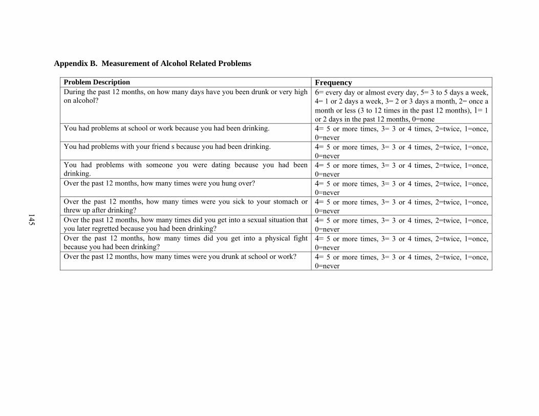
145
Appendix B. Measurement of Alcohol Related Problems
Problem Description Frequency During the past 12 months, on how many days have you been drunk or very high on alcohol?
6= every day or almost every day, 5= 3 to 5 days a week, 4= 1 or 2 days a week, 3= 2 or 3 days a month, 2= once a month or less (3 to 12 times in the past 12 months), 1= 1 or 2 days in the past 12 months, 0=none
You had problems at school or work because you had been drinking. 4= 5 or more times, 3= 3 or 4 times, 2=twice, 1=once, 0=never
You had problems with your friend s because you had been drinking. 4= 5 or more times, 3= 3 or 4 times, 2=twice, 1=once, 0=never
You had problems with someone you were dating because you had been drinking.
4= 5 or more times, 3= 3 or 4 times, 2=twice, 1=once, 0=never
Over the past 12 months, how many times were you hung over? 4= 5 or more times, 3= 3 or 4 times, 2=twice, 1=once, 0=never
Over the past 12 months, how many times were you sick to your stomach or threw up after drinking?
4= 5 or more times, 3= 3 or 4 times, 2=twice, 1=once, 0=never
Over the past 12 months, how many times did you get into a sexual situation that you later regretted because you had been drinking?
4= 5 or more times, 3= 3 or 4 times, 2=twice, 1=once, 0=never
Over the past 12 months, how many times did you get into a physical fight because you had been drinking?
4= 5 or more times, 3= 3 or 4 times, 2=twice, 1=once, 0=never
Over the past 12 months, how many times were you drunk at school or work? 4= 5 or more times, 3= 3 or 4 times, 2=twice, 1=once, 0=never

146
Appendix C. Illicit Drug Use
Types of Drug Value Since June 1995, have you taken any of the following drugs without a doctor’s permission? Sedatives or downers, such as barbiturates, sleeping pills, or Seconal? Yes=1, No=0 Tranquilizers, such as Librium, Valium, or Xanax? Yes=1, No=0 Stimulants or uppers, such as amphetamines, Prelud in, or speed? Yes=1, No=0 Pain killers, such as Darvon, Demerol, Percodan, or Tylenol with codeine? Yes=1, No=0 Steroids or anabolic steroids? Yes=1, No=0 Since June 1995, have you used any kind of cocaine—including crack, freebase, or powder? Yes=1, No=0 Since June 1995, have you used crystal meth? Yes=1, No=0 Since June 1995, have you used any other types of illegal drugs, such as LSD, PCP, ecstasy, Yes=1, No=0 mushrooms, inhalants, ice, heroin, or prescription medicines not prescribed for you?