steering performance dependence on...
TRANSCRIPT

STEERING PERFORMANCE DEPENDENCE ONFRONT SUSPENSION DESIGNMaster’s thesis in Automotive Engineering
JOACIM GILLBERGDIEGO ZAPARDIEL
Department of Applied MechanicsCHALMERS UNIVERSITY OF TECHNOLOGYGoteborg, Sweden 2015


MASTER’S THESIS IN AUTOMOTIVE ENGINEERING
STEERING PERFORMANCE DEPENDENCE ON FRONT SUSPENSIONDESIGN
JOACIM GILLBERGDIEGO ZAPARDIEL
Department of Applied MechanicsDivision of Vehicle Engineering and Autonomous Systems
Vehicle Dynamics GroupCHALMERS UNIVERSITY OF TECHNOLOGY
Goteborg, Sweden 2015

STEERING PERFORMANCE DEPENDENCE ON FRONT SUSPENSION DESIGNJOACIM GILLBERGDIEGO ZAPARDIEL
c© JOACIM GILLBERG, DIEGO ZAPARDIEL, 2015
Master’s thesis 2015:64ISSN 1652-8557Department of Applied MechanicsDivision of Vehicle Engineering and Autonomous SystemsVehicle Dynamics GroupChalmers University of TechnologySE-412 96 GoteborgSwedenTelephone: +46 (0)31-772 1000
Cover:Regression surface for maximum force in the rack.
Chalmers ReproserviceGoteborg, Sweden 2015

STEERING PERFORMANCE DEPENDENCE ON FRONT SUSPENSION DESIGNMaster’s thesis in Automotive EngineeringJOACIM GILLBERGDIEGO ZAPARDIELDepartment of Applied MechanicsDivision of Vehicle Engineering and Autonomous SystemsVehicle Dynamics GroupChalmers University of Technology
Abstract
’Steering performance parameters’ are the measures defined in this thesis to quantify the steering behaviorof vehicles. The parameters are important for the earlier stages of the design process and therefore a goodunderstanding on how these parameters may change when designing the suspension is vital. The objective ofthis work is to establish a general frame that describes the relation between the steering performance parametersand the suspension design factors regardless of the suspension type.
The work was done by studying one steering performance parameter, namely forces in the steering rackunder a simulated driving condition. A population of different suspension configurations with different designfactors was studied. A model of a McPherson suspension, including both kinematics and steering forces, wasdeveloped in Matlab to simulate these scenarios and gather all the necessary data for the study. Differentsuspension configurations with different design factors were simulated in this environment and the output forcesand other steering parameters were statistically post processed to find trends and confidence intervals to findthe relations.
The objective of the statistical analysis was to find a model that isolated the effect of each suspensiondesign factor on the different steering performance parameters. Linear regression models were used to fit thedata and variability of the estimators was specially studied.
The result of the study evidenced the difficulty of this problem. There is only statistically significant re-lation between castor trail and castor angle with all the steering performance parameters studied. Thestatistical study also reveals a close relation of the suspension design factors between themselves and the samefor the steering performance parameters.
Keywords: Steering, Suspension, McPherson, Steering performance, Suspension design factors, On-centre steer,Simulation.


Preface
This thesis is done as a part of the Master of Science in Automotive Engineering programme at ChalmersUniversity of Technology, Gothenburg. The project topic is proposed by LeanNova Engineering A.B., Trollhattan.The thesis work was performed between January 2015 and June 2015 at LeanNova and Chalmers.
Acknowledgements
First of all, we would like to express our gratitude to LeanNova and especially Gunnar Olsson for initiatingthe project. Also, we would like to thank our supervisors Oskar Eklund and Erik Hartelius, at LeanNova, forvaluable inputs and guidance during the thesis work.
Moreover we would like to extend our appreciation to Anders Bostrom at Chalmers for the guidance ofrigid body dynamics and Sergei Zuyev at Chalmers for the support around the statistical study part of thework.
Last but not least we would like to thank Bengt Jacobson at Chalmers for his help and guidance throughoutthe work.
iii


Nomenclature
Symbols
ay - Lateral acceleration [m/s2]B - Euler-Rodrigues rotation matrixf - Constraints vectorFly - Lateral force from Pacejka (Y-direction) left wheel[N]Flz - Vertical normal force (Z-direction) left wheel[N]Fry - Lateral force from Pacejka (Y-direction) right wheel [N]Frz - Vertical normal force (Z-direction) right wheel [N]Fsteering - Force in track rod [N]Fy - Lateral force (y-direction) [N]g - Gravity constant [m/s2]h1...h8 - Hardpoint coordinates in global reference system~h4′ - New position of the strut upper mount point when body rollhCoG - Centre of gravity height [m]Jf - Jacobian of fk - Longitudinal slip [%]L′ - New strut length after roll [mm]Lst - Strut length [mm]m - Mass of the whole car [kg]MZ - Self-aligning torque [Nm]~Mδ - Moment around the steering axis [Nm]O′ - Origin of local reference system after rollpx - Roll gradient [deg/g]~q1... ~q8 - Position vector for the hard points in the local referance systemR2 - Coefficient of determinationR - Rotation matrix for body rollRchassis - Reaction force upper strut mounting point [N]Re - Loaded wheel radiusRlca - Reaction force lower control arm outer ball joint [N]−−→rOm - Position vector for the origin of the local reference systemRw - Characteristic length of the lower control armtol - Tolerance value for Newton-Raphsonv - Velocity [km/h]w - Track width [m]X - Solution vector for Newton-Raphson
α - Slip angle [deg]δ - Steering axis~λ - Steering axis direction unit vectorφ - Roll angle [deg]
v

Abbreviations
CAD - Computer Aided DesignCoG - Centre of GravityEHPS - Electro-Hydraulic Power SteerEPS - Electric Power SteerGND - GroundHP - Hard Points (suspension/steering)HPS - Hydraulic Power SteerKPIA - Kingpin Inclination AngleKPO - Kingpin OffsetPSO - Particle Swarm OptimizationRC - Roll CentreSDF - Suspension Design FactorsSPP - Steering Performance ParameterSUV - Sport Utility VehicleVIF - Variability Inflation FactorWC - Wheel Centre
vi

Contents
Abstract i
Preface iii
Acknowledgements iii
Nomenclature v
Contents vii
1 Introduction 11.1 Background . . . . . . . . . . . . . . . . . . . . . . . . . . . . . . . . . . . . . . . . . . . . . . . . . 11.2 Problem Definition . . . . . . . . . . . . . . . . . . . . . . . . . . . . . . . . . . . . . . . . . . . . . 11.3 Objective . . . . . . . . . . . . . . . . . . . . . . . . . . . . . . . . . . . . . . . . . . . . . . . . . . 21.4 Deliverables . . . . . . . . . . . . . . . . . . . . . . . . . . . . . . . . . . . . . . . . . . . . . . . . . 21.5 Delimitations . . . . . . . . . . . . . . . . . . . . . . . . . . . . . . . . . . . . . . . . . . . . . . . . 21.6 Method . . . . . . . . . . . . . . . . . . . . . . . . . . . . . . . . . . . . . . . . . . . . . . . . . . . 2
2 Theory 52.1 Coordinate Systems . . . . . . . . . . . . . . . . . . . . . . . . . . . . . . . . . . . . . . . . . . . . 52.2 Suspension Design Factors . . . . . . . . . . . . . . . . . . . . . . . . . . . . . . . . . . . . . . . . . 62.3 Suspension Layout . . . . . . . . . . . . . . . . . . . . . . . . . . . . . . . . . . . . . . . . . . . . . 82.4 Steering Performance Parameters . . . . . . . . . . . . . . . . . . . . . . . . . . . . . . . . . . . . . 92.5 Mathematical Problem . . . . . . . . . . . . . . . . . . . . . . . . . . . . . . . . . . . . . . . . . . . 92.5.1 Numerical Methods For Equations Solving . . . . . . . . . . . . . . . . . . . . . . . . . . . . . . 102.6 Pacejka Tire Model . . . . . . . . . . . . . . . . . . . . . . . . . . . . . . . . . . . . . . . . . . . . . 11
3 Kinematic Model 133.1 Kinematic Study Purpose . . . . . . . . . . . . . . . . . . . . . . . . . . . . . . . . . . . . . . . . . 133.2 Geometrical Relations . . . . . . . . . . . . . . . . . . . . . . . . . . . . . . . . . . . . . . . . . . . 133.3 SDF Calculation . . . . . . . . . . . . . . . . . . . . . . . . . . . . . . . . . . . . . . . . . . . . . . 153.4 Matlab Implementation for the Kinematic Model . . . . . . . . . . . . . . . . . . . . . . . . . . . . 173.5 Validation of the Kinematic Model . . . . . . . . . . . . . . . . . . . . . . . . . . . . . . . . . . . . 18
4 Front Axle Model 194.1 Quarter Car Model . . . . . . . . . . . . . . . . . . . . . . . . . . . . . . . . . . . . . . . . . . . . . 194.2 Front Axle Study . . . . . . . . . . . . . . . . . . . . . . . . . . . . . . . . . . . . . . . . . . . . . . 204.3 Tire Model Calculation . . . . . . . . . . . . . . . . . . . . . . . . . . . . . . . . . . . . . . . . . . 214.4 Matlab Implementation for the Force Model . . . . . . . . . . . . . . . . . . . . . . . . . . . . . . . 224.5 Total Calculation Setup . . . . . . . . . . . . . . . . . . . . . . . . . . . . . . . . . . . . . . . . . . 23
5 Analyzing the Gathered Data 275.1 Data Analysis and parameters selection . . . . . . . . . . . . . . . . . . . . . . . . . . . . . . . . . 275.2 Statistical Study . . . . . . . . . . . . . . . . . . . . . . . . . . . . . . . . . . . . . . . . . . . . . . 28
6 Results 316.1 Suspension Model . . . . . . . . . . . . . . . . . . . . . . . . . . . . . . . . . . . . . . . . . . . . . 316.2 Statistic Result . . . . . . . . . . . . . . . . . . . . . . . . . . . . . . . . . . . . . . . . . . . . . . . 31
7 Conclusions and Future Work 357.1 Conclusions . . . . . . . . . . . . . . . . . . . . . . . . . . . . . . . . . . . . . . . . . . . . . . . . . 357.2 Future Work . . . . . . . . . . . . . . . . . . . . . . . . . . . . . . . . . . . . . . . . . . . . . . . . 36
Bibliography 37
vii
A Vehicle data 3
B Matlab Program Manual 5
C Matlab Model Code 7C.1 Matlab main program . . . . . . . . . . . . . . . . . . . . . . . . . . . . . . . . . . . . . . . . . . . 7C.2 Initial condition . . . . . . . . . . . . . . . . . . . . . . . . . . . . . . . . . . . . . . . . . . . . . . . 15C.3 SDF . . . . . . . . . . . . . . . . . . . . . . . . . . . . . . . . . . . . . . . . . . . . . . . . . . . . . 16C.4 Roll to travel . . . . . . . . . . . . . . . . . . . . . . . . . . . . . . . . . . . . . . . . . . . . . . . . 17C.5 myfunsyms . . . . . . . . . . . . . . . . . . . . . . . . . . . . . . . . . . . . . . . . . . . . . . . . . 17C.6 Newton-Raphson . . . . . . . . . . . . . . . . . . . . . . . . . . . . . . . . . . . . . . . . . . . . . . 18C.7 Transformation . . . . . . . . . . . . . . . . . . . . . . . . . . . . . . . . . . . . . . . . . . . . . . . 19C.8 Lateral load transfer . . . . . . . . . . . . . . . . . . . . . . . . . . . . . . . . . . . . . . . . . . . . 19C.9 Magic formula . . . . . . . . . . . . . . . . . . . . . . . . . . . . . . . . . . . . . . . . . . . . . . . 20C.10 Force in the rack . . . . . . . . . . . . . . . . . . . . . . . . . . . . . . . . . . . . . . . . . . . . . . 21C.11 interpo . . . . . . . . . . . . . . . . . . . . . . . . . . . . . . . . . . . . . . . . . . . . . . . . . . . . 22
D Statistical Data 23D.1 Lateral acceleration at maximum force . . . . . . . . . . . . . . . . . . . . . . . . . . . . . . . . . . 23D.2 Drop rate (acceleration) . . . . . . . . . . . . . . . . . . . . . . . . . . . . . . . . . . . . . . . . . . 27D.3 Drop rate (slip angel) . . . . . . . . . . . . . . . . . . . . . . . . . . . . . . . . . . . . . . . . . . . 30D.4 Maximum force in the steering rack . . . . . . . . . . . . . . . . . . . . . . . . . . . . . . . . . . . 33D.5 On-centre slip angle . . . . . . . . . . . . . . . . . . . . . . . . . . . . . . . . . . . . . . . . . . . . 37D.6 On-centre rate (acceleration) . . . . . . . . . . . . . . . . . . . . . . . . . . . . . . . . . . . . . . . 40D.7 Slip angle for maximum force . . . . . . . . . . . . . . . . . . . . . . . . . . . . . . . . . . . . . . . 43
viii

Chapter 1
Introduction
1.1 Background
Steering performance is an important field of study among automotive engineers since it is a key factor invehicle handling and driver feel. Steering performance can be divided into vehicle steering response andsteering feel. Steering performance is measured in Steering performance parameters (SPP). The industryprovides steering assistance solutions such as Hydraulic power steering (HPS), electric power steering (EPS)and electro-hydraulic power steering (EHPS) which reduces driver effort, thereby increasing driver comfort. Theinterest on sustainable transportation in cities is making car manufacturers invest in small, light-weight andcheap vehicles where HPS, EPS and EHPS are desirably avoidable to reduce costs. This makes it interesting tostudy how to influence the steering performance characteristics just by changing suspension hardpoints andthus suspension design factors (SDF). Exampels of SDFs are given in 2.2.
These SDF can be seen as an universal communication vehicle between automotive engineers. This is veryuseful when sharing information regardless of the platform or suspension type you are working with as it ispossible to define these factors for all of them through their different geometries.
Literature on this topic is not abundant, and even less so for the approach presented in this work. Ro-hit Vaidya et al. [1] studied the on-centre handling behavior of vehicles depending on six different vehiclecharacteristics although not suspensions design factors. Ragnar Ledesma and Shan Shih [2] studied the effectof steering axis inclination angle and wheel offset on medium-duty truck handling and found clear relationsbetween these two factors and the steering responses that they studied. R. P. Rajvardhan et al. [3] studied theeffect of wheel geometry parameters on vehicle steering using a model of a SUV type vehicle in ADAMS/CAR,a multibody dynamics software used in the automotive industry. Skip Essma [4] wrote about the steering effortevaluation and modification for a Champ Car type of vehicle. He studied the change in steering effort whilemodifying camber, castor and castor trail. Yung-Hsiang Judy Hsu and J. Christian Gerdes [5] studied the peaklateral performance and handling limit estimation through steering torque. The lack of information on SDFsimpact on SPPs motivates this study. It is important to highlight that this work tries to find a general frameto describe the relation between SDFs and SPPs for any kind of vehicle, independent of suspension type.
1.2 Problem Definition
All car manufacturers have their own ideas and philosophies when setting the targets for the suspension designfactors. For achieving these target numbers based on the suspension design different computer software isavailable. However, these computer software do not give a clear general correlation between the SDFs andthe SPPs. Therefore this master thesis project is proposed to provide this correlation of suspension designfactors and steering performance parameters of a vehicle. This is useful for the engineers designing suspensionsystems and will help them to set these design targets in the future. With this knowledge the engineers can,independent of the suspension type, find what to change in the suspension to achieve a desired value for asteering performance parameter. Also the communication between engineers will be improved due to the factthat SDFs says more of a suspension than just hardpoints positions and configurations in space. A benefit ofSDF as opposed to hardpoints is that suspensions of different suspension types can be compared, e.g. a certainMcPherson can be compered with a certain Double Wishbone.
1

In Figure 1.1 a basic scheme shows how the suspension and steering hardpoints (HP) gives the SDFs which thengives a specific steering performance. Some examples of SDFs are toe angle, camber angle and the kinematicvariations of these, like ride camber, ride toe, track width change, etc..
Figure 1.1: Vehicle Steering Performance Parameters, SPPs.
1.3 Objective
The main purpose of this master thesis is to create an understanding of how the suspension design factors, givenby the front suspension geometry, affect the steering performance of the vehicle. This understanding is providedby studying trends in steering performance when changing suspension hardpoints for a fixed suspension type ina statistical environment.
1.4 Deliverables
The deliverables of this thesis are:
• Computer program to simulate/calculate SDF from HP
• Computer program to sweep HP and analyze correlation between SDF and SPP
• Computer program to simulate/calculate SPP from SDF
• A report summarizing the study and the results
• A manual for the computer programs
1.5 Delimitations
Although the study is intended for all suspension types in this project a McPherson suspension of a front wheeldriven car is used as a base. The study only focuses on front steering cars without power steering systems andthe effects produced in the intermediate shaft and steering column. The focus of the study lies on the frontaxle, thus the theoretical model in this thesis will be a half-car model.
In this thesis only steering force related SPPs were studied and at a significant velocity (v > 25km/h)[6], so no parking forces or low speed manoeuvrability is taken into account. The scenarios studied and modelused applied to passenger vehicles.
To get a real in-depth understanding of the suspension and steering system functionality the suspensionmodel will be developed in Matlab instead of using a commercial multi-body (black box) software.
1.6 Method
A complete model was done in Matlab. Starting from a set of hardpoints (of an already existing suspension)the first step was to create a kinematic model. the next step was to calculate the SDFs for the entire movementof the suspension. This included bump, rebound and steering motions, both individual and combinations ofthem. Multi body simulation data was provided by LeanNova Engineering AB to verify the results.
By implementing the tire and input forces (in this case a high speed turning driving scenario) the car
2

experiences a lateral acceleration and roll motion. The correct suspension travel left/right shall be calculatedfor this roll and then the net force in the rack can be calculated using the resulting suspension geometry.
By varying the hardpoints of the suspension model, resulting in changed SDFs, it was possible to studythe net rack force versus lateral acceleration and thereby find the relation between SPPs and SDFs. A databasewith all the different suspension configurations was created. Each entry contained information about thehardpoints, the SDFs and the SPPs for a certain configuration. This database was statistically post processedto find a model that directly relates SPPs and SDFs.
An alternative method that could have been used is to use a conventional multi body program to cre-ate the database that then could be evaluated using statistical methods. This was never an option because itwas set as a delimitation. This was because it would not give a good enough understanding of the relationbetween suspension hardpoints and suspension characteristics (SDFs) and their correlation [7]. Real vehicletesting methods could have also been thought of for this work but since the intention was to obtain a generalframe valid for any type of suspension and configuration it would take a huge amount of time and money totest a sufficient population of vehicles to draw conclusions.
3


Chapter 2
Theory
2.1 Coordinate Systems
The coordinate systems used in this thesis follow the ISO 8855-standard [8] as defined below.
Intermediate axis system
The X and Y axis are parallel to the ground plane and the Z axis is orthogonal to this one. The X-axis ispointing forward in the car’s direction and the Y-axis is pointing left of the car’s direction. The Z-axis ispointing upwards. This is illustrated in Figure 2.1.
Figure 2.1: ISO 8855 vehicle and intermediate axis systems.
Tire and wheel axis system
The tire and wheel axis system in this thesis is according to ISO 8855 and is illustrated in Figure 2.2. Thesubscript T stands for the tire and the subscript W stands for wheel.
Figure 2.2: ISO 8855 tire and wheel axis system.
5

2.2 Suspension Design Factors
The suspension design factors are defined by the suspension hardpoints. The relevant SDFs for this thesis aredefined in this section. These SDFs are chosen mostly for their direct relation with the steering axis. Camberand toe are included for validation purposes and future implementation in a tire model.
Camber angle at design loadThe camber angle is the angle between the Z-axis and the centreline through the wheel in the car’s Y-Zplane. If the wheel is leaning inwards to the car this angle is defined negative and if it is leaning outwardsit is positive. This is illustrated in Figure 2.3.
Figure 2.3: Wheel seen in the Y-Z plane to illustrate camber.
Steering axisThe steering axis is defined as the axis around which the steering takes places. For example in a McPhersonsuspension the upper mounting point is the top strut and the lower outer hardpoint is the lower controlarm outer ball joint.
CastorCastor angle is the angle between the steering axis (seen in the X-Z plane) and the Z-axis. This is illustratedin Figure 2.4.
Figure 2.4: Wheel seen in the X-Z plane to illustrate castor.
Castor offset at wheel centreSpindle trail
The castor offset is the distance given by the centre line of the wheel (Z-axis) and the steering axis seen inthe X-Z plane (castor axis). Therefore the castor offset at wheel centre is the distance orthogonal to thewheel centre line in Z-direction to the castor axis in the wheel centre point. This is illustrated in Figure2.4.
6

Castor offset at groundCastor trail, kinematic trail
The castor offset at ground is the orthogonal distance to the centre line of the wheel in Z-direction to thecastor axis at ground level. This is illustrated in Figure 2.4.
Steering axis inclination angleKingpin inclination angle, KPIA
The steering axis inclination angle is the angle given by steering axis seen in the Y-Z plane and the centreline through the wheel. This is illustrated in Figure 2.5.
Figure 2.5: Wheel seen in the Y-Z plane to illustrate steering axis inclination angle and its offsets.
Steering axis offset at wheel centreKingpin offset at wheel centre
The kingpin offset is the distance given by the centre line of the wheel (Z-axis) and steering axis seen inthe Y-Z plane. Therefore the kingpin offset at wheel centre is the distance orthogonal to the wheel centreline in Z-direction to the kingpin axis in the wheel centre point. This is illustrated in Figure 2.5.
Steering axis offset at groundKingpin offset at ground
The kingpin offset at ground is the distance orthogonal to the centre line of the wheel in Z-direction to thekingpin axis at ground level. This is illustrated in Figure 2.5.
7

Static toe angle
The Static toe angle is the angle generated by the offset of the wheel centerline (X-direction) and theX-axis of the vehicle, see Figure 2.6. It is considered positive when the wheel centreline leans towardsthe vehicle and negative when it leans outwards. Total static toe angle is defined for steering rack in thecentre position, meaning that is a design measure for the axle, not the wheel.
Figure 2.6: Wheel seen in the X-Y plane to illustrate toe, sign definition valid for both view from above (leftwheel) and from under (right wheel).
2.3 Suspension Layout
The suspension used as base in this thesis is a front suspension of McPherson type. The base hardpoints arefrom a front wheel drive car. There are eight different hardpoints that are of significant interest for the studyof this thesis. With these hardpoints it is possible to reproduce the whole suspension movement and calculateall the SDFs described in chapter 1. They are specified in Table 2.1 and illustrated in Figure 2.7.
Figure 2.7: Figure of suspension with hardpoints.
Table 2.1: Table showing the hardpoints
h1 Lower wishbone front pivoth2 Lower wishbone rear pivoth3 Lower wishbone outer ball jointh4 Strut upper mount pointh5 Strut slider upper axis pointh6 Outer track rod ball jointh7 Inner track rod ball jointh8 Wheel centre point
It is possible to divide the hardpoints in two different groups depending on whether they are part of the sprungor unsprung mass. This is of importance further in the thesis to calculate the position of the suspension whenthe car rolls. h1, h2, h4 and h7 are the hardpoints fixed to the body (sprung mass). The rest of the hardpoints,h3, h5, h6 and h8, form part of the unsprung mass and will remain in their position with body roll (since ridetoe effect is not considered).
8

2.4 Steering Performance Parameters
The steering performance parameters to be studied in this thesis are all related to steering force in the rack,Figure 2.8. This means that the study is more driver-focused than vehicle-focused. Maximum force in the rackis an interesting parameter to study because it can be useful for design engineers to dimension the steeringsystem. Force increment rate is also studied at low slip angles. This rate works as a parameter to measure theon centre steering feel and it is representative for most of the time driving a passenger vehicle at high speed.The rate at which force goes down when the vehicle loses grip is another parameter studied. This rate is usefulto provide a measure of how the driver feels that the steering torque decreases, and although this is not such acommon situation as straight driving, it occurs when driving in icy conditions or during evasive maneuvers.The last parameter studied is the maximum acceleration before losing grip. This last one is more performanceorientated and tells how much grip is possible to gain through the suspension geometry. Depending on theintention of the vehicle, race car or passenger vehicle, the objective for these parameters may vary. This thesisis focused on passenger vehicles.
Figure 2.8: SPPs in Rack force VS slip angle.
2.5 Mathematical Problem
In a McPherson suspension all the links are joined to the knuckle. The real system is constrained so that everyposition of the knuckle corresponds to a unique position of the whole suspension system. By knowing theposition and orientation of the knuckle the coordinates of all hardpoints can then be found.
The knuckle has six degrees of freedom, three translational motions in X, Y, Z and three rotational mo-tions around X, Y, Z. The local system defined in chapter 3 has the same degrees of freedom since it is fixed tothe knuckle. To know the position and orientation of this local system a system of six equations is needed. Sincerotation is also involved there will be trigonometrical equations between these six so the mathematical problemto solve is a system of six non-linear equations. To make the formulation in Matlab easier the parametricvariant of the Euler-Rodrigues rotation matrix is used instead of the angular one. This matrix uses the classicRodrigues’ rotation formula but including Euler notation, and is used to calculate rotation of bodies in threedimensional space. This parametrical formulation gives both an extra variable and an extra equation so thefinal problem is a system of seven non-linear equations. Further study of this kinematic problem is presented inChapter 3.
9

2.5.1 Numerical Methods For Equations Solving
In numerical analysis there are different types of algorithms to solve mathematical problems, from simplelinear equations to complex large systems of non-linear equations. The simplex method is the most usedfor linear problems but it is of no interest for this thesis since the problem to solve here is non-linear. It ispossible to separate the non-linear algorithms in two groups: gradient-free algorithms and gradient-basedalgorithms. The first kind is used when the constraints cannot be differentiated well from the objective andare generally approximation models that start with a random input and look for trends that improve theinitial input iteratively until a satisfactory solution is found. Some examples of gradient-free algorithms arethe Pattern search algorithm, Particle swarm optimization (PSO) and genetic or evolutionary algorithms [9].Since the mechanical problem studied in this thesis is well constrained, and the equations are differentiable, agradient-based algorithm is employed since it is way faster and accurate. The most used method in this group,and the one chosen for this project, is the Newton-Raphson method. This algorithm requires an initial pointclose to the solution to assure convergence and that the solution found is the one looked for (see Figure 2.9).
Figure 2.9: Importance of initial conditions for non-linear functions
Since the initial design layout of our problem is given, and the movement starts from this position in a continuousway, the initial point is not an issue. An iteration example is shown in Figure 2.10. The mathematical formulationfor this algorithm is shown in Equations 2.1-2.2.
Xn+1 = Xn − [Jf (Xn)]−1 · f(Xn) (2.1)
||[Jf (Xn)]−1 · f(Xn)|| < tol (2.2)
10

Figure 2.10: Algorithm approximation to solution
Where X is the vector of solutions (or initial conditions in the first iteration), f is the vector containing theconstraint functions and J is the jacobian matrix of f. tol is the value of the maximum tolerance desired.
2.6 Pacejka Tire Model
It is necessary for this study to adopt a tire model capable to give lateral force and self-aligning torque for acertain vertical load and slip angle. This force and torque is used to calculate the SPPs. Other authors havestudied tire behavior and have developed different tire models like Dugoff et al. [10] and Bernard et al. [11].Existing models vary from empirical to purely physical and the purpose of the study determines which methodis best. In this thesis the objective is not to study the tire itself so the in depth physical study of the tire isnot of interest. The tire model adopted is the Magic Formula [12], of the semi-empirical type. This modelis conceived to present the tire as a component for a simulation environment, thus is computationally fastand intended for the steady-state calculations carried away in this work. Since only high speed maneuvers areaimed for (chapter 1) it is not necessary to include the spin torque and the Magic Formula is sufficient to coverthe thesis needs.
Pacejka’s model is solely based in empirical data from tire tests. The data is statistically treated so thatfinally a regression model that adjusts to the reality is created. The coefficients of the regression model have aphysical meaning making the magic formula a very used model as it provides physical information about tirecharacteristics as well as it faithfully reproduces the tire behavior. Expression 2.3 shows the simplest variant ofthe magic formula. This expression can be equalled to longitudinal force, lateral force or self-aligning torquedepending on the coefficients used.
D sin(C arctan(B α+ E (arctan(B α)−B α))) (2.3)
with stiffness factor B, peak factor D, cornering stiffness factor C and curvature factor E. Depending on thevalues used for the different coefficients the magic formula yields longitudinal force, lateral force or self-aligningtorque. Equations 2.4 to 2.8 show how these factors are calculated for lateral force and self-aligning torque [13].
D = a1 · FZ2 + a2 · FZ (2.4)
11

C =
{1.3 Numerical value for Lateral force
2.4 Numerical value for Self-aligning torque(2.5)
B · C ·D =
{a3 sin (a4 tan (a5 · FZ)) Lateral forcea3·FZ
2+a4·FZ
ea5·FZ
Self-aligning torque(2.6)
B =B · C ·DC ·D
(2.7)
E = a6 · FZ2 + a7 · FZ + a8 (2.8)
Where a1. . . a8 are the coefficients that give the dependency with normal load (see Table 2.2) [13].
Table 2.2: Normal load coefficients.
a1 a2 a3 a4 a5 a6 a7 a8Fy -22.1 1011 1078 1.82 0.208 0 -0.354 0.707Mz -2.72 -2.28 -1.86 -2.73 0.110 -0.07 0.643 -4.04
12

Chapter 3
Kinematic Model
3.1 Kinematic Study Purpose
Given a set of hardpoints for the front suspension, the kinematics of all these hardpoints has to be calculatedin order to know the position of the suspension throughout the wheel travel and steering maneuver. Thehardpoints positions (X-, Y- and Z-positions) were taken from a CAD software and the programs made in thethesis were made with these hardpoints as the main input.
3.2 Geometrical Relations
The knuckle is the solid body in which the interest is focused since this is the part that carries the wheel andwill define its movement. To study the movement of this part (that will immediately give the movement of thewhole suspension system) a typical approach in rigid body dynamics was used [14]. A local reference systemwas defined so it was possible to work with both global and local coordinates. To ease the calculations thislocal reference system was defined as fixed to the knuckle. The Z’ direction was chosen to be the one of thestrut, the X’ was obtained as the cross product of the directional vector of the track rod and the Z’ and finally,the Y’ was defined as the cross product of Z’ and X’ to make the reference system orthogonal and right handed.This is illustrated in Figure 3.1.
Figure 3.1: Ilustration of the local reference system in the knuckle, front view.
It is possible to determine the movement of the knuckle by knowing, for each instant, the position andorientation of the local reference system, given a series of constraints. The local reference system has six degreesof freedom so a set of six constraint equations must be found. Using the Euler-Rodrigues rotation matrix Bin its parametric form (eq. 3.1) introduced another variable in the system. The new equation needed is thetrigonometry relation between this new variable and the other three Euler parameters (eq. 3.2).
B =
2 e02 + 2 e1
2 − 1 2 e1 e2 − 2 e0 e3 2 e0 e2 + 2 e1 e32 e0 e3 + 2 e1 e2 2 e0
2 + 2 e22 − 1 2 e2 e3 − 2 e0 e1
2 e1 e3 − 2 e0 e2 2 e0 e1 + 2 e2 e3 2 e02 + 2 e3
2 − 1
(3.1)
e02 + e1
2 + e22 + e3
2 = 1 (3.2)
13

where e0 is the cosine of half the rotated angle and [e1 e2 e3] is the unit vector of the rotation axis times thesine of half of the rotated angle.
These movement constraints were mathematically treated using vectors. The length constraints were specifiedby the magnitude of certain vectors and the fixed movements were set by means of scalar product as is shownin the following equations. “q” vectors were referred to the local system and “r” vectors to the global system.Figure 3.2 shows the points used in the calculations
Figure 3.2: Points used in the movement and SDFs calculations.
For the lower control arm there are two constraints (equations 3.3 and 3.4): the fixed length of the arm andthe plane of the movement respectively. This plane is the one whose normal is the axis defined by the controlarm front and rear pivots in the chassis and passes through h3.
∣∣∣∣∣∣−−→rOm− ~rO + B · ~q3∣∣∣∣∣∣− Rw = 0 (3.3)
(~h1− ~h2
) (−−→rOm− ~rO + B · ~q3
)∣∣∣∣∣∣ ~h1− ~h2
∣∣∣∣∣∣ = 0 (3.4)
14

For the track rod the length is set as a fixed value (equation 3.5).
∣∣∣∣∣∣−−→rOm− ~h7 + B · ~q6∣∣∣∣∣∣− Rs = 0 (3.5)
The remaining three constraints come from the strut (equations 3.6 - 3.8). The length of the strut, even thoughit was the parameter that varied during the simulation itself, it was a fixed value in each simulation step. Thelast two constraints came from the orientation of the strut in the local reference system. The strut has to beperpendicular in every step to the Y’ and X’ axis so this gave the two remaining constraints.
∣∣∣∣∣∣ ~h4−−−→rOm
∣∣∣∣∣∣− Lst2 = 0 (3.6)
B · (1, 0, 0)′ · ( ~h4−−−→rOm) = 0 (3.7)
B · (0, 1, 0)′ · ( ~h4−−−→rOm) = 0 (3.8)
The variable parameter selected as input for the mathematical model was the length from the strut toppoint to the origin of the local reference system. By changing this parameter, which can be viewed as a changein the spring length (compression caused by a change in road elevation for instance), the different positions ofthe suspension system were calculated.
3.3 SDF Calculation
According to the objective of the thesis (Chapter 1) it was necessary to calculate the suspension design factorsto investigate how the SPPs are related to them and draw conclusions regarding this relation. The main SDFsof interest for this study were the ones directly related to the steering axis. Change in steering axis producesthe most significant change in steering performance of the vehicle. Steering axis inclination angle as well asits ground offset and wheel centre offset were studied. Separating front view and side view it was possible todifferentiate six different SDFs. Seen in the X-Z plane (side view) these were the castor angle, castor offset atground and castor offset at wheel centre. For the front view the SDFs were the steering axis inclination angle,steering axis offset at ground and steering axis offset at wheel centre [8].
Apart from the mentioned parameters and for validation purposes the toe and camber angles were alsocalculated to compare them with the data from the multi body software. The results of the calculations ofthese SDFs are the ones illustrated in Figure 3.3.
15

Figure 3.3: How the SDFs change due to positive (> 0) and negative (< 0) wheel travel
The steering axis offsets at wheel centre were calculated using the normal vector to the axis that passes throughthe wheel centre (rsteerWC). This vector was calculated by finding the intersection point between the steering
axis and a plane containing the wheel centre, with the steering axis unit vector (~λ) as its normal vector.Equations 3.9 to 3.11 shows how this point was calculated.
~λ =~h4− ~h3∣∣∣∣∣∣ ~h4− ~h3
∣∣∣∣∣∣ (3.9)
A =
1 0 0 −λ(1)0 1 0 −λ(2)0 0 1 −λ(3)
λ(1) λ(2) λ(3) 0
(3.10)
b =
h3Xh3Yh3Z~λ · ~h8
(3.11)
The first three rows of A and b correspond to the parametric equations of the steering axis in 3-D andthe fourth row to the equation of the plane. By solving the system of equations in equation 3.12 it was possibleto obtain the wheel center point, OWC , by taking the first three components of x.
A · x = b (3.12)
16

The vector used to calculate the SDFs later on was calculated in equation 3.13
rsteerWC = (OWC − h8) (3.13)
All of these SDFs were calculated as follows (equations 3.14 - 3.19):
Steering axis inclination angle (KPIA) = arctan
(h4Y − h3Yh4Z − h3Z
)(3.14)
Steering axis offset at WC =√rsteerWC(3)2 + rsteerWC(2)2 (3.15)
Steering axis offset at GND = tan(KPIA) ·(Re − h8Z − h3Z +
(h3Y − h8Ytan(KPI)
))(3.16)
Castor angle = − arctan
(h3X − h4Xh4Z − h3Z
)(3.17)
Castor offset at WC =√rsteerWC(3)2 + rsteerWC(1)2 (3.18)
Castor offset at GND = tan
(Castorangle ·
(Re +
(h3X − h8Xtan(castor)
)+ h8Z − h3Z
))(3.19)
3.4 Matlab Implementation for the Kinematic Model
Figure 3.4 shows the process followed with the Matlab script to calculate the coordinates of the suspensionthroughout the wheel travel. This flowchart with the loop is meant to calculate the hardpoints for a wheeltravel of ±100mm from the design positions just for plotting and validation purposes. Further on in the projectwhen a certain position was needed to make calculations the loop was no longer needed since it was only usedfor calculating a whole range. If the length parameter L0 was known beforehand for a certain position it couldbe directly used as an input without starting from the beginning and doing all the loops. This length parameterwas the distance between the strut top mount point and the origin of the local reference system, as defined onchapter 2
Figure 3.4: Flowchart for the Kinematic Model
17

The first function (block A) calculates the seven constraints for the mechanism given a series of hardpoints andlengths. The points fixed to the chassis were expressed in global coordinates and the ones in the unsprungmass were expressed in the local reference system. The lengths defined were the track rod, the lower controlarm characteristic length and the strut input length parameter L0. The output of this function was a vector ofseven equations and seven unknowns that made a system to be solved in the next step.
The Newton-Raphson function (block B) calculates the solution for the constraints system of equationsusing the iterative Newton-Raphson calculation process explained in the theory chapter 2. A vector X0 wasused as initial position and from this point the algorithm iterated until the error became smaller than thetolerance value and at that point the solution was given. For each step in the simulation of the suspensionmovement, the initial position vector X0 used was the position calculated in the previous step. By doing thisthe number of iterations the solver requires was reduced and computation time was saved. It was also a way toensure the convergence of the algorithm.
The output of the Newton-Raphson function was a seven components vector containing the global posi-tion of the local system of reference and the coefficients in the rotation matrix for the local reference system fora certain amount of wheel travel.
Finally this vector was used as an input for the last function (block C). This transformation function calculatesthe moving hardpoint coordinates first in the local system and then transforms the coordinates to the globalsystem. The final output was a matrix with the global coordinates of all eight hardpoints used.
3.5 Validation of the Kinematic Model
The validation process was necessary to be able to rely on the created model and use the data extracted from itwith confidence. The validation process chosen involved both visual and numerical procedures. For the visualpart an animation of the suspension moving in bump and steer was performed to confirm/verify the model.This first verification permited to check in a quick glimpse if there were major errors and it was not compareddirectly with any real animation from multi body software. The comparisons with the multi body softwarewere done through the SDF plots gotten from our Matlab model and the ones from the multi body softwareshown in figure 3.5.
Figure 3.5: Kinematic SDF for developed Matlab model (blue) and multi body simulation (red).
By inspecting that the kinematic model worked correctly it was possible to proceed with the study and startlooking into the forces in the rack. With the maximum lateral acceleration the roll of the body produced abump/rebound of 38mm in the suspension. In this range of wheel travel (±38mm) the maximum relative errorfor camber was 1.7% and for toe 2%. This deviation far from zero travel might be explained by the fact thatthe multibody simulation includes bushing deflections while the Matlab model did not include them. The restof the SDFs were in the same range of relative error.
18

Chapter 4
Front Axle Model
4.1 Quarter Car Model
To ease the calculations, and since the origin of the tire forces is not a main part of this thesis, an ideal scenariowas used to calculate the forces into the system. The front axle was modeled as fixed to a fictitious test rig,Figure 4.2. This rig sits on a directional rolling band which gives the wheel both slip angle and angular speed.The steering was locked so there was no translation of the rack when the forces were calculated.
If the wheel and spindle were considered as a continuous solid system (this is neglecting the stiffness ofthe tire) it was possible to define its two degrees of freedom: wheel travel and rotation around steering axis.Since longitudinal forces and torques in the hub or brake discs were not studied the rotation of the wheel wasnot considered.
The system had an applied force and three reaction forces applied in four points: tire patch, lower control armball joint, track rod outer ball joint and strut top point. To get the steering rack force, the force at the track rodwas the one that needed to be calculated. Tire patch forces and self-aligning torque were known but the rest werenot. This problem was solved by doing the momentum equilibrium study around the steering axis (Equation 4.1).
∑~Mδ = ( ~MZ · ~λ)~λ+ ~F × ~r + ~Fsteering × ~r2 = 0 (4.1)
Since the forces from the strut and the lower control arm to the spindle were applied in points of the steeringaxis (momentum equals zero) this left the force in the track rod as the only unknown. With the force in thetrack rod calculated, the force in the rack was obtained just by projecting the former on the rack axis (Y-axis).
Figure 4.1: Free body diagram of one side of the suspension
19

4.2 Front Axle Study
To compute the net force in the rack it was necessary to take into account both right and left wheels. Withlateral force and lateral acceleration comes body roll and load transfer which broke the symmetry and caused anet force to appear in the rack that was felt in the steering wheel. Due to body roll the geometry of the innerand outer suspension was different (bump and rebound) and due to load transfer the inner and outer lateralforce and self-aligning torque were also different. Figure 4.2 shows the fictitious rig that provides this load case.
Figure 4.2: Illustration of the half-car rig
For the body roll study, and since the objective of this thesis was not getting exact values but trends,a roll gradient (px) of 4 deg/g was used in the calculations [7]. The roll centre changed from one set ofhardpoints to another. On the other hand roll centre was assumed to be constant with body roll. Thisassumption was made due to time limitations [7] and taking into account that the conditions of the simulationsdid not involve body rolls greater than 3◦. Roll angle (φ) was calculated as in Equation 4.2:
Roll angle, φ = px ·ayg
(4.2)
With the roll angle it was possible to geometrically know the position of the strut upper point, h4′, since thispoint was fixed to the chassis. The origin of the local reference system (Om) did not move with the roll so withthese two points’ coordinates it was possible to obtain the length parameter to use in the kinematic model andobtain the rest of the points’ coordinates (Equations 4.3 – 4.5).
R =
(cos(φ) − sin(φ)sin(φ) cos(φ)
)(4.3)
20

~h4′ = R · ~h4 + ~RC (4.4)
L′ = ||h4′ −O′|| (4.5)
Figure 4.3: Illustration of the change of the suspension due to roll
R is the rotation matrix for the rolling chassis and RC is the position vector of the roll centre in the global system.
For a given lateral acceleration (ay) the lateral load transfer was calculated as in Equation 4.6 and Equation4.7 [15]:
Flz = m ·(g
2− ay ·
(hCoGw
))(4.6)
Frz = m ·(g
2+ ay ·
(hCoGw
))(4.7)
4.3 Tire Model Calculation
There are a lot of different variants of the basic magic formula which allows studying different tire situations.One example of this is the conicity and ply-steer effects of the tire that may introduce offsets near the origin ofcoordinates into the formula. These effects were not taken into account for the purpose of this thesis and sincethe work was done at zero camber the most basic version of the magic formula with no horizontal or verticalshifts was used. The lateral force Fy was then calculated from the magic formula in Equation 4.8.
Fy = DF sin(CF arctan(BF α+ EF (arctan(BF α)−BF α))) (4.8)
For the self-aligning torque MZ the same formula was used but with different coefficients, equation 4.9
MZ = DM sin(CM arctan(BM α+ EM (arctan(BM α)−BM α))) (4.9)
21

To calculate the input forces in the model this formula was used with the vertical load previously calcu-lated taking the load transfer into account and for a sweep of slip angles. Figures 4.4 and 4.5 show thecharacteristic lateral force and self-aligning torque for pure slip condition (longitudinal slip (k) = 0, no combinedslip).
Figure 4.4: Fy and MZ for the outer tire. Figure 4.5: Fy and MZ for the inner tire.
4.4 Matlab Implementation for the Force Model
The dynamic part of the Matlab program is meant to calculate the force in the rack. Figure 4.6 shows aflowchart of this Matlab model.
Figure 4.6: Flowchart for Force Model
The first function (block A) calculates the load transfer and the total vertical load in the two wheels given thelateral acceleration and vehicle data (centre of gravity height, track width, mass, et cetera.) given as inputs.
With the vertical load for both wheels in the front axle the second function (block B) implements themagic formula to calculate the lateral force and self-aligning torque that the wheel produced for that amount
22

of vertical load for a sweep of slip angles. According to the driving situation described both inner and outerwheels have the same slip angle since the road was the surface that changed direction. The lateral force in eachtire was calculated so that the sum of both tires at the same slip angles gave the total amount of lateral forceneeded to cope with the inertia of the vehicle (Equation 4.10).
Fly + Fry = m · ay (4.10)
The calculated force and self-aligning torque for the slip angle were used as input forces in the suspen-sion system and the third function (block C), using again the geometry from the vehicle data, calculates thenet force in the rack as shown in section 4.1.
4.5 Total Calculation Setup
The Matlab program as a whole works as described in the flowchart shown in Figure 4.7. The objective of theprogram is to gather data to see how forces in the rack change when changing hardpoints (and in consequencethe SDFs). To gather a database with a variation of SDFs and load cases, hardpoints in the base suspensionsystem were changed. There are three hardpoints that directly affect the chosen SDFs for this study: h3, h4and h8. The position of these three hardpoints was changed in each iteration of the script. H3 and h4 move inall X,Y and Z directions while h8 only moves in X and Y, as a movement in Z direction could be interpreted asa change in wheel size rather than in suspension geometry.
Figure 4.7: Flowchart for the general simulation
There are different design of experiments approaches to study a statistical phenomena. The most used are thefactorial experiments (full or fractional) and the randomized blocks.
For these movements a fractional factorial design was discarded since there was no clear variable or cor-relation that could be discarded at first hand. Besides, the low calculation time of the full factorial designmade the latter the chosen one.
Randomized blocks experiments such as the ones performed with latin hypercube generated data were alsodiscarded due to the low calculation time of the full factorial and the easiness of data analysis since all thefactors had a clearly stated variation values rather than random possibilities in a range. This type of experimentcould reduce the simulation runs to the half but as stated before, the time was not a problem. Furthermore, touse a Latin hypercube model the level two and three interactions had to be zero and it was not possible toaffirm it in this stage of the analysis.
23

The simulations were then carried out with a full factorial methodology in two phases. First the hard-points were changed 10mm in positive directions and then 10mm in negative directions, h3 and h4 were movedin X-, Y- and Z-direction but h8 was only changed in the X-Y plane (see Figure 4.8). The changing hardpointsmoved along the corners of the cubes and planes.
Figure 4.8: Illustration of how the hardpoints changes
This specific movement was chosen to remain in the design space of a vehicle. The changes could not be toobig but big enough to appreciate variation in the output. This gave 512 configurations of the suspension whichwas more than sufficient for the study [16].
Figure 4.9 shows an example of how the force in the rack changed when moving h3 +10mm in Z-direction. Thepeak force increased by ≈ 100N and both initial and final slope were steeper.
Figure 4.9: Different force in the rack when changing h3 in Z-direction
24
All this data was tabulated and for each hardpoints configuration it gave a certain value for the studied SDFsas well as the SPPs. The tabulated data was afterwards processed using JMP, a statistics software package, tosee the relation between the SPPs and the SDFs and to study how good a regression model could describethese phenomena.
25


Chapter 5
Analyzing the Gathered Data
5.1 Data Analysis and parameters selection
To evaluate the steering performance parameters it was necessary to define them. Figure 4.9 shows the netforce in the rack plotted against lateral acceleration for two hardpoints’ configurations. The shape of the curvesdoes not change from one set of hardpoints to the other. It was possible then to compare steering performancebetween different configurations by calculating the maximum values and rates. These parameters of study areshown in Figures 5.1 and 5.2. The first three values to study have to do with the maximum net force in therack. These are the maximum value of the force (A in Figure 5.1 and 5.2) as well as the slip angle and lateralacceleration at which this maximum force occurs (B in Figure 5.2 and E in Figure 5.1 respectively). Observingthe slopes it was possible to get information for the initial and final rates. Studying the region with small slipangles it was possible to define another parameter (C in Figure 5.2). This is the ascending force/slip rate anddescribes the on-centre feel. Studying the region with high slip angles the fifth and last parameter was defined,the drop rate (D in Figure 5.2). This last parameter is a way to identify the feeling in the steering wheel whenthe grip in the tires is lost.
Figure 5.1: SPPs in Rack force VS lateral acceleration. Figure 5.2: SPPs in Rack force VS slip angle.
Table 5.1: Table describing the SPPs
A Maximum force in the rackB Slip angle at which this maximum force is obtainedC Ascending force/slip angle rateD Drop rateE Lateral acceleration at which this maximum force is obtained
27

5.2 Statistical Study
The mechanical complexity of the problem made it really hard to isolate the effect of a particular SDF onthe SPPs (which is the main objective of the thesis). Taking this into account, the best way to approach theproblem and draw results was to statistically treat the obtained database and, through regression models, drawconclussions on the relation between SDFs and SPPs.
After running the simulations a database of 512 different suspension configurations was created with in-formation about the value of SPPs and SDFs for each and all of them.
The objective of the statistical study was to find a model that fitted the results obtained in the 512 Matlabsimulations and explained the correlation between each SDF and each SPP individually. Different models weremade for each SPP. The response variable of each regression model was the SPP studied and the regressors orestimators were the SDFs.
A regrassion model with all SDFs and significant interactions up to fourth grade is created for all theSPPs. The first thing to study was the coefficient of determination R2, which measures how well the data fittedthe model. As a general guideline it is possible to classify regression models oriented to prediction as shown inTable 5.2 [16].
Table 5.2: R square values classification.
< 0, 3 0, 3− 0, 4 0, 4− 0, 5 0, 5− 0, 85 > 0, 85Very bad Bad Regular Good Suspicious
Figure 5.3 shows the graphical representation of these regression models for maximum force. After eliminatingall estimators with t-statistic value under 2 (p-value > 0.05) it presented an R2 of 0.46 and adjusted R2 of0.44. This model was able to predict half of the variability of actual cases, and the prediction formula could beuseful but not a hundred percent reliable. In any case the aim of this thesis was not that much the predictionpotential of the model because it is obvious that a general formula capable of giving the SPP for any vehicledoes not exist. The focus was more in the structural behavior and the impact that the estimators have onthe response. Studying the p-value column in Table 5.3 it was possible to observe that all the SDFs have asignificant influence in the model except for the interactions Castor ∗ Castor offset at WC and Castor trail ∗Castor offset at WC. These two were not removed from the model because the adjusted R2 decreases by doingso.
Figure 5.3: Regression model for maximal force with all SDFs.
28

Table 5.3: Parameter estimates table.
The Correlation or Pearson matrix (Figure 5.4) was studied to find the relation and dependence of the designfactors and performance parameters in the raw data. A high correlation between the different SDFs was found.Taking only the submatrix for the SDFs it was possible to check for linear dependence between them by lookingat the value of the determinant of the matrix. For this case the value is in the order of magnitude of 10−5 whichclearly means that some of the estimators are strongly dependent [17]. This dependency was even emphasizedwhen observing the SPPs submatrix where the determinant value is approximately 10−10.
Table 5.4: Person matrix for raw data.
The Pearson matrix gives a hint of possible multicollinearity in the model. This is precisely what was notdesired in the results. Multicollinearity does not affect the predictability potential of the model but makes itharder to interpret the results and separate the role that the different estimators have in it. The model tries toseparate the effect of the estimators when in reality they are bound and redundant [17]. To go deeper intothis analysis and tell whether multicollinearity was present or not it was possible to look into diagnosis toolslike the VIF (variability inflation factor) for each estimator. This factor tells how much the standard errorof an estimator increases due to the effect of collinearity. Values above 10 for this factor are worrisome andindicate presence of collinearity [18]. Figure 5.3 shows the VIF value for the different estimators in the modeland it exceeded by far the value of 10 in practically all the cases. Leaving only the estimators with VIF valuebelow 10 in the model and eliminating the rest the coefficient of determination goes drastically down to 0.25which was a very poor value (Table 5.2). The estimators left out were castor and castor trail which are theonly two SDF moderately correlated with the SPPs according to the Pearson correlation matrix for the raw data.
The space for the data is a seven dimension space (six estimators and one response for each model). Reducingthe dimension of the study space coulde be useful for the comprehension of the problem and to get rid of someof the dependence of the variables. The scatter plots for different SDFs were studied to find patterns or rangesof values to divide the first big model into several models of smaller dimension. Scatter plots for castor (Figure
29

5.4) clearly presented three different ranges so new regression models were made for each different level.
Figure 5.4: Scatter plot for castor angle VS max net force in the rack.
These models seemed to give a better fit (between 0.65 and 0.85) but looking carefully into the estimators itwas found that they have high VIF values and unusually high coefficients values in the prediction formula. Thisis because the variance of the estimators depends on the inverse value of the determinant of the Pearson matrixfor the estimators which for this new model is around 10−13. This makes the variance approach infinity andmakes the estimators very sensitive to the sample and thus not accurate or precise. At this point, estimators donot give any relevant information. This can basically mean that the response variable has really no relation withthe estimators (which is not true because there is a physical relation) or it can also mean that the estimatorsused were redundant and highly correlated. Removing these estimators with high VIF from the model madethe trust curves tend asymptotically to the average as shown in Figure 5.5, which indicates that the model isnot significant.
Figure 5.5: Regression for 2◦, 3◦ and 4◦ castor angle
The 3◦ castor level is not that sensitive to removal of castor because the correlation between force and thisSDF at the 3◦ castor angle range is not significant.
30

Chapter 6
Results
6.1 Suspension Model
A working kinematic model has been made from scratch including the correct movement of the unsprungmass as well as the calculation of the forces in steering rack when applying a load case for a simulated lateralacceleration. As this thesis focuses on the study of trends and not exact values the model presented in thisthesis should be good enough to give an insight on what forces the steering rack feels under the simulatedscenarios.
6.2 Statistic Result
The scatter plots shown in Figure 6.1 confirm that there is only relation of the SPPs with castor and castortrail.
Figure 6.1: Scatter plots for Castor angle and Castor trail VS maximum force in rack.
Observing the correlation matrix for the raw data with all the SPPs and the SDFs, it was possible to see thatthe SPPs depend only with a correlation of 0.45 and 0.3 with the castor and castor trail. With the rest ofSDFs the correlation is less than 0.15 in most cases. These correlation values support the results given by themodels studied when cutting by planes of constant castor and castor trail. The relation left between the SDFsand the SPPs is so small, when taking out of the equation castor and castor trail, that the model loses itssignificance as shown in Figure 5.4. Another interesting result that could be obtained from the Pearson matrixis that all the studied SPPs are highly correlated with a value for the correlation coefficient above 0.9 for allcases, so the study of the trends and the structural behavior of the problem could be done studying only one ofthe different SPPs. The individual study of all of them would only make sense if the objective was obtainingthe different coefficients for the prediction formulas but since the models explain only the 25% of the variabilitythis formulas were better not used.
31

Figure 6.2 shows the regression model for max force with only castor and castor trail as regressors. Bothregressors are significant in this model and there is no trace of collinearity. The numerical values of thecoefficients for the estimators lack of interest because of the low R2.
Figure 6.2: Regression model for max force with castor and castor trail as regressors.
The response surface of this model (Figure 6.3) tells that the relation of the maximum force in the rack, and byextension of all the SPPs, is positive with castor angle and castor trail. This means that increasing these twoSDFs will result in an increased value of maximum force in the rack.
Figure 6.3: Regression surface for maximum force in the rack.
32

Another result derived from the statistical study is the evidence of correlation existence between SDFs. Figure6.4 shows both the relation between KPO at ground and KPO at wheel centre and the absence of relationbetween these two SDFs and the SPPs.
Figure 6.4: Correlation between KPO at WC and KPO at GND.
33

Chapter 7
Conclusions and Future Work
7.1 Conclusions
The results shown in Chapter 6 may suggest that different SDFs should have been chosen when preparingthe study or that there is no general correlation between the SDFs and SPPs studied. It is logical that theestimators are highly correlated because they are all geometric parameters of the wheel steering axis. It is thenobvious that changing angles will have an effect in offsets and the other way around. Thus it is difficult toisolate the effect of only one parameter.
The study of the correlation of the SDFs leaves only two variables (castor and castor trail) to study aphenomenon that depends on a lot of different things, and the model shows that two variables is not sufficientto explain most of the variability of the SPPs (only 25%). It will be necessary to introduce new SDFs to use asestimators to create a better model capable of explaining the relation between SPPs and SDFs. This argumentsupports the idea that the poor results obtained, in terms of explaining the correlation, are more likely causedby the lack of studied SDFs than the evidence of a non existing relation.
It is important to not forget that this master thesis tries to explain how SPPs vary in a very generalframework. That is regardless of the type of suspension and other parameters. It is clear that, within a vehicle,conclusions can be drawn about each and every one of the SDFs leaving the rest fixed. For example an increasein suspension arm’s length will mean higher forces, et cetera. But in a general case you cannot establish a directrelation based on a database that does not take into account all the parameters that affect the system. In thiswork for example the steering arm length, which is a key parameter, is not being taken into account so thereforeis not possible to say with confidence what the dependence is between the different SPPs with the SDFs aswe cannot know the relation between these SDFs and the steering arm (or the rest of the non-consideredparameters). There are two different ways of acting on this problem: keeping all the non studied SDFs constantor monitoring their changes and include them in the statistical study.
It is possible to discuss whether the method chosen for the realization of the thesis has been adequate.A lot of time has been invested preparing the Matlab model capable of generating all the data required for thestudy. This has made the time available to prepare simulations very limited. Having started from scratch usinga multi body program would have been beneficial to obtain the necessary database for the study and the timeand effort could have been focused more on results than on preparing the Matlab model. On the other handfollowing this methodology would imply losing the learning advantages in using Matlab. Making a simulationenvironment of a suspension helps to understand how it works and this learning is very beneficial facing thedesign of these systems.
The results obtained are not quite the ones expected at the begining of the work. The lack of literatureregarding this topic makes it necessary to dig into an unknown field and the expectations change quickly.Rather than conclude that the results are bad it is possible to say that this thesis is only the tip of the icebergof a way bigger problem and with this previous study done, and the computer models already developed itstands like a good starting point to keep working on the project.
35

7.2 Future Work
It is possible to improve the method in all its stages and keep going on obtaining more valuable results out ofthe topic of this master thesis. The primary points where it is necessary to take action are:
• Introduce more SDFs in the study and analyze their effect, the steering arm being the most relevant
• Verify the force calculations to be sure of its outcome
• Rethink the way of obtaining the statistical population. Aim for a random distribution to avoid repeatedand ranged output.
• Minor implementations to the calculation such as including camber, ride toe, rear axle, roll centremovement, etc.
There are more design factors that affect the steering performance parameters than the ones studied in thisthesis. By implementing these desing factors the result will be more accurate and will show relations that arehidden when only studying the six SDFs chosen for this work. The main new design factor to take into accountis the steering arm lenght. Adding this new design factor will add the most effective information that will havea positive impact on the results. A validation of the force model similar to the one made with the kinematicmodel is needed to get more trustworthy results.
A new way of getting the statistical population to analyze is needed to further improve the results. Therecommendation here is to forget the full factorial design and go for a bigger population of random configurationsin a wider range of movement for each hardpoint ( ±20mm instead of ±10mm for example). This way repeatedoutput is avoided and the complete database will have more useful information.
There are several other things that can be implemented into the model. The change of camber that iscreated by the wheel travel is one thing that can be implemented by expanding the tire model. The kinematicsof this change is already in the model but was not considered due to time limitations. To be able to investigatemore SDFs and SPPs a whole car should be implemented into the model, this meaning implementing a rearaxle. It will be possible then to add the effect of ride toe to the steering of the wheels. Ride toe already existsin the kinematic model but without a rear axle it cannot be implemented. Roll centre movement with roll isanother improvement to implement into the model.
36

Bibliography
[1] R. Vaidya, P. Seshu, G. Arora, Study of on-center handling behaviour of a vehicle.
[2] R. Ledesma, S. Shih, The effect of kingpin inclination angle and wheel offset on medium-duty truckhandling, Tech. Rep. 2001-01-2732, SAE technical paper series (2001).
[3] R. Rajvardhan, Effect of wheel geometry parameters on vechilce steering, Master’s thesis, Ramaiah Schoolof Advanced Studies, Bangalore (09 2010).
[4] S. Essma, Steering effort analysis of an oval racing track setup champ car (2000).
[5] Y.-H. J. Hsu, J. C. Gerdes, The predictive nature of pneumatic trail: tire slip angle and peak forceestimation using steering torque, Tech. rep., Stanford University (2008).
[6] B. Jacobson, Professor in Vehicle Dynamics, Chalmers University of Technology, 2015.
[7] G. Olsson, Senior Integration Engineer, Adjunct Professor of Vehicle Dynamics, LeanNova EngineeringAB, Chalmers University of Technology, 2015.
[8] J. Y. Wong, Road vehicles – Vehicle dynamics and road-holding ability – Vocabulary (ISO 8855:2011,IDT), 2nd Edition, Swedish Standards Institude, 2012.
[9] P. Y. Papalambros, D. J. Wide, Principles of Optimal Design : Modeleing and Computation, Cambridge :Cambridge University Press, 2000.
[10] D. et al., Tire performance characteristics affecting vehicle response to steering and braking control inputs,final report, Tech. rep., Highway Safety Research Institute, Ann Arbor, Michigan (1969).
[11] B. et al., Tire shear force generation during combined steering and braking maneuvers, Tech. Rep. 770852,SAE technical paper (1977).
[12] H. B. Pacejka, Tyre and vehicle dynamics, Elsevier Butterworh-Heinemann, 2004.
[13] J. G. de Jalon, Formula magica de pacejka, Lecture notes for the course Metodos Matematicos deEspecialidad (2007).
[14] A. B. et al, Rigid body dynamics, Chalmers University of Technology, 2013.
[15] B. J. et al, Vehicle Dynamics, Compendium for Course MMF062, Chalmers University of Technology,2012.
[16] J. M. R. Abuin, Regresion lineral multiple, Tech. rep., Instituto de Economia y Geografia, Madrid, Spain(2007).
[17] R. Stine, Colinearity and multiple regression (2001).
[18] S. O’Halloran, Lecutre 5: Model checking.
37


Appendices


Appendix A
Vehicle data
Table A.1: Table showing Vehicle data
mass (front) 945 kgroll gradient 4 deg/gwheel radius loaded 289 mmtrack width 1.5 mCOG height 0.5 m
Table A.2: Table showing the hard points original position (NOT ACCORDING TO ISO)
Hard point X-coordinate [mm] Y-coordinate [mm] Z-coordinate [mm]h1 1660.748 -393.961 151.0192h2 1959 -378 160.5h3 1721.542 -724.545 142.444h4 1758.84 -572.697 798.379h5 1735.09 -600.87 377.53h6 1862.58 -693.74 239.33h7 1898.0 -317.5 245.0h8 1728.1 -756.71 259.1
3


Appendix B
Matlab Program Manual
This appendix is a manual for the usage of the matlab code for further development. In chapters threeand four we explained the flow of the matlab script with the help of several flowcharts. This manual isuseful to let the user know where to change parameters and which parts to keep untouched. The code iscommented so most of the information can be directly extracted from the program. The script starts withthe definition of the constants that will take part in the program. Here it is possible to change vehiclecharacteristics such as mass, CoG height, etc. Base hard points should also be changed here. H3, h4 and h8can be directly modified in the main script. To modify the rest of the hard points step in function ‘initcondition’.
The preallocation of matrices should not be changed unless the number of the steps for the simulationsis changed. In that case just adjust each case for the number of simulations desired. All the For..if..else loopsthat come after are just to change the hard points to get all the simulations. All this loops can be taken outand changed for some other kind of code capable of generate different hard point’s configurations to do thecalculations. If the loops are to be kept it is possible to change the amplitude of the movement by changing the‘10’ for any other value.
Here the main part of the program where all the calculations are done starts. First of all the ‘SDF’ functioncalculates the SDFs for the configuration of hard points for an iteration. You can add more SDFs as output forthis function if desired and add more points or geometrical information if it is necessary to calculate these newSDFs.
After the SDFs for the static case are calculated we proceed to apply lateral acceleration. The positionof the body due to body roll is obtained with the function ‘roll2travel’. This function gives the length parameterfor both inner and outer wheels to use later in the kinematics and obtain the whole suspension position for acertain amount of lateral acceleration.
The next two sections calculate the position of the suspension for inner and outer wheel as described onchapter 3. Nothing must be changed here unless the user wants to change the type of suspension to study.After the suspension position is known we proceed to calculate the forces in the system. Lateral load transferis calculated and the output values of vertical load for inner and outer wheel are used as inputs for the‘magicformula’ function to calculate lateral force and self-aligning torque that the wheel is capable of generatingfor that load and a sweep of slip angles. The range of slip angles studied is specified in the ‘magicformula’function. To change this value go into the function and change the alpha value set for default as linspace(0,15).In the ‘magicformula’ function the shifts Sh and Sv can be uncommented to add camber effect and other wheeleffects. The camber should be declared as the second input variable for this function. With the forces andself-aligning torque in the tire patch now we calculate the forces into the suspension system as described onchapter 4. The function ‘forceinrack’ calculates the force in the rack with the previously calculated M innerand suspension position. Same is done for the outer wheel.
With both calculated it is possible to calculate the overall force in the rack and plot it against lateralacceleration. Add or comment plots in the plots section and the same for entries to be done in the database
5

Appendix C
Matlab Model Code
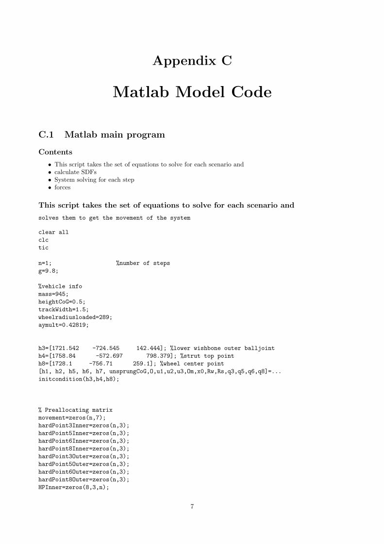
C.1 Matlab main program
Contents
• This script takes the set of equations to solve for each scenario and• calculate SDFs• System solving for each step• forces
This script takes the set of equations to solve for each scenario and
solves them to get the movement of the system
clear all
clc
tic
n=1; %number of steps
g=9.8;
%vehicle info
mass=945;
heightCoG=0.5;
trackWidth=1.5;
wheelradiusloaded=289;
aymult=0.42819;
h3=[1721.542 -724.545 142.444]; %lower wishbone outer balljoint
h4=[1758.84 -572.697 798.379]; %strut top point
h8=[1728.1 -756.71 259.1]; %wheel center point
[h1, h2, h5, h6, h7, unsprungCoG,O,u1,u2,u3,Om,x0,Rw,Rs,q3,q5,q6,q8]=...
initcondition(h3,h4,h8);
% Preallocating matrix
movement=zeros(n,7);
hardPoint3Inner=zeros(n,3);
hardPoint5Inner=zeros(n,3);
hardPoint6Inner=zeros(n,3);
hardPoint8Inner=zeros(n,3);
hardPoint3Outer=zeros(n,3);
hardPoint5Outer=zeros(n,3);
hardPoint6Outer=zeros(n,3);
hardPoint8Outer=zeros(n,3);
HPInner=zeros(8,3,n);
7

HPOuter=zeros(8,3,n);
uWheel=zeros(n,3);
factor=zeros(256,9);
maxforce=zeros(256,1);
slip=zeros(256,1);
slope=zeros(256,1);
ForceInner=zeros(100,3);
M_Inner=zeros(100,3);
ForceOuter=zeros(100,3);
M_Outer=zeros(100,3);
slipVSay=zeros(21,1);
ForceVSay=zeros(21,1);
latacc=zeros(21,1);
for i=1:2
if i==1
h8(1)=h8(1)-10;
else
h8(1)=h8(1)+10;
end
for j=1:2
if j==1
h8(2)=h8(2)-10;
else
h8(2)=h8(2)+10;
end
for k=1:2
if k==1
h4(1)=h4(1)-10;
else
h4(1)=h4(1)+10;
end
for l=1:2
if l==1
h4(2)=h4(2)-10;
else
h4(2)=h4(2)+10;
end
for ii=1:2
if ii==1
h4(3)=h4(3)-10;
else
h4(3)=h4(3)+10;
end
for jj=1:2
if jj==1
h3(1)=h3(1)-10;
else
8

h3(1)=h3(1)+10;
end
for kk=1:2
if kk==1
h3(2)=h3(2)-10;
else
h3(2)=h3(2)+10;
end
for ll=1:2
if ll==1
h3(3)=h3(3)-10;
else
h3(3)=h3(3)+10;
end
calculate SDFs
[steeringAxisInclinationAngle,steeringAxisOffsetwc,castor,...
castorTrail,steeringAxisOffsetgnd,...
steeringAxisInclinationAngleSide,steeringAxisOffsetwcSide]=...
SDF(h3,h4,h8,n,uWheel,wheelradiusloaded);
for iiii=0:20
%initialize conditions
[ LstInner, LstOuter, h4Outer, h4Inner ] = roll2travel( aymult*iiii,h1,h3,h4,h5,Om );
h4Outer=[h4(1); h4Outer]’; h4Inner=[h4(1); h4Inner]’;
System solving for each step
for iii=1:1
[phi1, phi2, phi3, phi4, phi5, phi6, phi7]=...
myfunsyms(LstInner,O,Rw,Rs,q3,q6,h1,h2,h4,h7);
F=vpa([phi1, phi2, phi3, phi4, phi5, phi6, phi7]);
movement(iii,:)=newtonraphson(F,x0,0.000001,20);
[HPInner(:,:,iii),uWheel(iii,:)]=...
transformation(movement(iii,:),q3,q5,q6,q8,h1,h2,h4,h7,u3,u2,u1);
hardPoint3Inner(iii,:) = HPInner(3,:,iii);
hardPoint5Inner(iii,:) = HPInner(5,:,iii);
hardPoint6Inner(iii,:) = HPInner(6,:,iii);
hardPoint8Inner(iii,:) = HPInner(8,:,iii);
end
for iii=1:1
[phi1, phi2, phi3, phi4, phi5, phi6, phi7]=myfunsyms(LstOuter,O,Rw,Rs,q3,q6,h1,h2,h4,h7);
F=vpa([phi1, phi2, phi3, phi4, phi5, phi6, phi7]);
movement(iii,:)=newtonraphson(F,x0,0.000001,20);
[HPOuter(:,:,iii),uWheel(iii,:)]=...
transformation(movement(iii,:),q3,q5,q6,q8,h1,h2,h4,h7,u3,u2,u1);
hardPoint3Outer(iii,:) = HPOuter(3,:,iii);
hardPoint5Outer(iii,:) = HPOuter(5,:,iii);
hardPoint6Outer(iii,:) = HPOuter(6,:,iii);
9

hardPoint8Outer(iii,:) = HPOuter(8,:,iii);
end
forces
LateralForce=mass*aymult*iiii;
[normalLoadLeft, normalLoadRight] =...
lateralLoadTransfer(mass,heightCoG,trackWidth,aymult*iiii);
[FxInner,FyInner,MzInner,~,~] = magicFormula(normalLoadLeft/1000,0,1);
uw=(h4Inner-hardPoint3Inner)/norm(h4Inner-hardPoint3Inner); %steering axis
A=[ 1 0 0 -uw(1)
0 1 0 -uw(2)
0 0 1 -uw(3)
uw(1) uw(2) uw(3) 0];
b=[ hardPoint3Inner(1) hardPoint3Inner(2) hardPoint3Inner(3) ...
dot(uw,hardPoint8Inner-[0 0 wheelradiusloaded])]’;
M1=A\b;
O_tp=(M1(1:3))’;
r_steer_tirepatchInner= (O_tp-(hardPoint8Inner-[0 0 wheelradiusloaded]));
for q=1:100
ForceInner(q,:)=[0 FyInner(q) normalLoadLeft];
momentInner=(cross(ForceInner(q,:),r_steer_tirepatchInner)*uw’)*uw;
selfAligningInner=([0 0 -MzInner(q)*1000]*uw’)*uw;
% moment_coordinatesInner=dot(momentInner,uw);
M_Inner(q,:)= selfAligningInner+momentInner;
end
f_rackInner=...
forceinrack(M_Inner,ForceInner,hardPoint3Inner,h4Inner,hardPoint5Inner,...
hardPoint6Inner,h7,hardPoint8Inner);
[FxOuter,FyOuter,MzOuter,~,alphaRange] = magicFormula(normalLoadRight/1000,0,1);
uwO=(h4Outer-hardPoint3Outer)/norm(h4Outer-hardPoint3Outer); %steering axis
uwO(2)=-uwO(2);
A2=[ 1 0 0 -uwO(1)
0 1 0 -uwO(2)
0 0 1 -uwO(3)
uwO(1) uwO(2) uwO(3) 0];
b2=[ hardPoint3Outer(1) -hardPoint3Outer(2) hardPoint3Outer(3)...
dot(uwO,[hardPoint8Outer(1) -hardPoint8Outer(2) hardPoint8Outer(3)]-[0 0 wheelradiusloaded])]’;
M2=A2\b2;
O_tp_Outer=(M2(1:3))’;
r_steer_tirepatchOuter= (O_tp_Outer-([hardPoint8Outer(1) -hardPoint8Outer(2) hardPoint8Outer(3)]-...
[0 0 wheelradiusloaded]));
for q=1:100
ForceOuter(q,:)=[0 FyOuter(q) normalLoadRight];
momentOuter=(cross(ForceOuter(q,:),r_steer_tirepatchOuter)*uwO’)*uwO;
selfAligningOuter=([0 0 -MzOuter(q)*1000]*uwO’)*uwO;
% moment_coordinatesOuter=dot(momentOuter,uwO);
10

M_Outer(q,:)=selfAligningOuter+momentOuter;
end
f_rackOuter=...
forceinrack(M_Outer,ForceOuter,hardPoint3Outer,h4Outer,...
hardPoint5Outer,hardPoint6Outer,h7,hardPoint8Outer);
f_rack= f_rackInner-f_rackOuter;
LateralForceTire=FyOuter+FyInner;
x=find(LateralForceTire>=LateralForce,1);
slipVSay(iiii+1)=alphaRange(x);
ForceVSay(iiii+1)=f_rack(x);
latacc(iiii+1)=iiii*aymult;
end
ayFine = 0:0.005:aymult*20;
forceVSayFine = spline(latacc,ForceVSay,ayFine);
slipVSayFine = spline(latacc,slipVSay,ayFine);
figure (1)
plot(ayFine,forceVSayFine)
title(’Force in Rack against lateral acceleration’)
xlabel(’lateral acceleration [m/s^2]’)
ylabel(’Rack force [N]’)
grid on
hold on
figure (2)
plot(slipVSayFine,forceVSayFine)
title(’Force in Rack against slip angle’)
xlabel(’slip angle [deg]’)
ylabel(’Rack force [N]’)
grid on
hold on
figure (3)
plot(slipVSayFine,ayFine)
title(’lateral acceleration against slip angle’)
xlabel(’slip angle [deg]’)
ylabel(’lateral acceleration [m/s^2]’)
grid on
hold on
[F_max,pos]=max(forceVSayFine(:,:));
indexx=(i-1)*2^7+(j-1)*2^6+(k-1)*2^5+(l-1)*2^4+(ii-1)*2^3+(jj-1)*2^2+(kk-1)*2+(ll-1)*1;
index=[ ’id’, num2str(indexx)];
DATA.(index).HardPointsInner=HPInner;
DATA.(index).HardPointsOuter=HPOuter;
DATA.(index).SDF=[steeringAxisInclinationAngle,steeringAxisOffsetwc,castor,...
castorTrail,steeringAxisOffsetgnd,...
steeringAxisInclinationAngleSide,steeringAxisOffsetwcSide];
DATA.(index).A=F_max;
DATA.(index).B=ayFine(pos);
DATA.(index).C=(forceVSayFine(1713)-forceVSayFine(1635))/(slipVSayFine(1713)-slipVSayFine(1635));
11
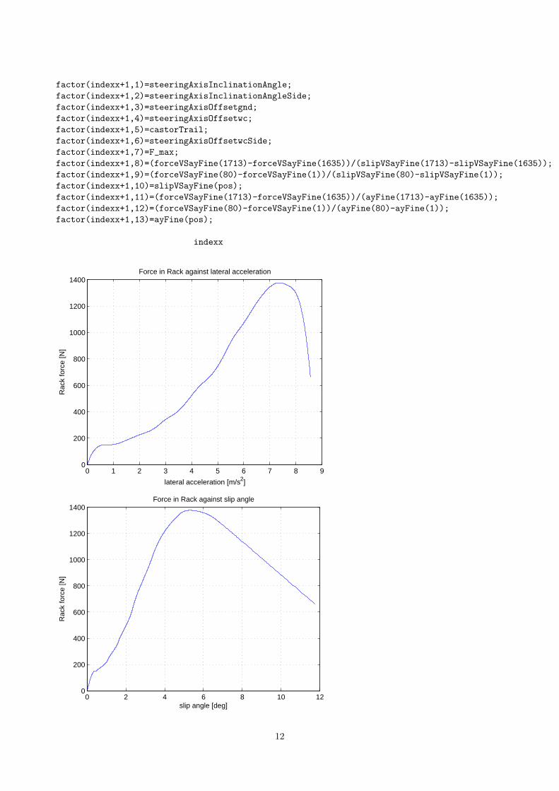
factor(indexx+1,1)=steeringAxisInclinationAngle;
factor(indexx+1,2)=steeringAxisInclinationAngleSide;
factor(indexx+1,3)=steeringAxisOffsetgnd;
factor(indexx+1,4)=steeringAxisOffsetwc;
factor(indexx+1,5)=castorTrail;
factor(indexx+1,6)=steeringAxisOffsetwcSide;
factor(indexx+1,7)=F_max;
factor(indexx+1,8)=(forceVSayFine(1713)-forceVSayFine(1635))/(slipVSayFine(1713)-slipVSayFine(1635));
factor(indexx+1,9)=(forceVSayFine(80)-forceVSayFine(1))/(slipVSayFine(80)-slipVSayFine(1));
factor(indexx+1,10)=slipVSayFine(pos);
factor(indexx+1,11)=(forceVSayFine(1713)-forceVSayFine(1635))/(ayFine(1713)-ayFine(1635));
factor(indexx+1,12)=(forceVSayFine(80)-forceVSayFine(1))/(ayFine(80)-ayFine(1));
factor(indexx+1,13)=ayFine(pos);
indexx
0 1 2 3 4 5 6 7 8 90
200
400
600
800
1000
1200
1400Force in Rack against lateral acceleration
lateral acceleration [m/s2]
Rac
k fo
rce
[N]
0 2 4 6 8 10 120
200
400
600
800
1000
1200
1400Force in Rack against slip angle
slip angle [deg]
Rac
k fo
rce
[N]
12

0 2 4 6 8 10 120
1
2
3
4
5
6
7
8
9lateral acceleration against slip angle
slip angle [deg]
late
ral a
ccel
erat
ion
[m/s
2 ]
0 1 2 3 4 5 6 7 8 90
200
400
600
800
1000
1200
1400
1600Force in Rack against lateral acceleration
lateral acceleration [m/s2]
Rac
k fo
rce
[N]
13

0 2 4 6 8 10 120
200
400
600
800
1000
1200
1400
1600Force in Rack against slip angle
slip angle [deg]
Rac
k fo
rce
[N]
0 2 4 6 8 10 120
1
2
3
4
5
6
7
8
9lateral acceleration against slip angle
slip angle [deg]
late
ral a
ccel
erat
ion
[m/s
2 ]
end
end
end
end
end
end
end
end
t=toc
% plot(F_max,ForceVSay)
% figure (2)
% plot(latacc,slipVSay)
14

% title(’Force in Rack against slip angle at design height’)
% xlabel(’slip angle [deg]’)
% ylabel(’Rack force [N]’)
% grid on
% hold on
C.2 Initial condition
Contents
• point O• point Om• fixed lengths• Movable hardpoints coordinates in Local system
function [h1, h2, h5, h6, h7, unsprungCoG,O,u1,u2,u3,Om,x0,Rw,Rs,q3,q5,q6,q8]=initcondition(h3,h4,h8)
h1=[1660.748 -393.961 151.0192]; %lower wishbone front pivot
h2=[1959. -378. 160.5]; %lower wishbone rear pivot
h5=[1735.09 -600.87 377.53]; %strut slider upper axis point
h6=[1862.58 -693.74 239.33]; %outer track rod ball joint
h7=[1898.0 -317.5 245.0]; %inner track rod ball joint 317.5
unsprungCoG=[1728.1-1 -756.71+5 259.1]; %wheel center point
point O
uw=(h1-h2)/norm(h1-h2); %Rotation axis of the wishbone
% wpn=cross(h1-h3,h2-h3)/norm(cross(h1-h3,h2-h3)); %normal vetor of wishbone plane
% nplane=cross(uw,wpn); %vector normal to the wishbone axis and contained in the plane
A=[ 1 0 0 -uw(1)
0 1 0 -uw(2)
0 0 1 -uw(3)
uw(1) uw(2) uw(3) 0
];
b=[ h2(1) h2(2) h2(3) dot(uw,h3)]’;
M=A\b;
O=(M(1:3))’;
% Point calculated as an intersection of axis 1-2 and a plane perpendicular and containing h3
point Om
u1=(h4-h5)/norm(h4-h5);
uaux=(h7-h6)/norm(h7-h6);
u3=cross(uaux,u1);
u2=cross(u1,u3);
A2=[ 1 0 0 -u1(1)
0 1 0 -u1(2)
0 0 1 -u1(3)
u1(1) u1(2) u1(3) 0
];
b2=[h4(1) h4(2) h4(3) dot(u1,h6)]’;
M2=A2\b2;
Om=(M2(1:3))’;
% Point calculated as an intersection of axis 4-5 and a plane perpendicular and containing h6
15

x0=[1726.391 -611.190 223.473 1 0 0 0]; %initial conditions for the solver
fixed lengths
Rw=norm(h3-O); % wishbone caracteristic length
Rs=norm(h6-h7); % steering rod length
Movable hardpoints coordinates in Local system
q3=[u3’ u2’ u1’]’*(h3-Om)’; %Base change matrix * vector in global coordinates
q5=[u3’ u2’ u1’]’*(h5-Om)’;
q6=[u3’ u2’ u1’]’*(h6-Om)’;
q8=[u3’ u2’ u1’]’*(h8-Om)’;
C.3 SDF
function [steeringAxisInclinationAngle,steeringAxisOffsetwc,castor,...
castorTrail,steeringAxisOffsetgnd,...
steeringAxisInclinationAngleSide,steeringAxisOffsetwcSide]=...
SDF(hardPoint3,h4,hardPoint8,~,~,wheelradiusloaded)
% camber=-atand((hardPoint8(:,2)-hardPoint3(:,2))./(hardPoint8(:,3)-hardPoint3(:,3)));
% toe=asind(uWheel(:,1)./sqrt((uWheel(:,1)).^2+(uWheel(:,2)).^2));
steeringAxisInclinationAngle=atand((h4(2)-hardPoint3(:,2))./(h4(3)-hardPoint3(:,3)));
steeringAxisInclinationAngleSide=atand((h4(1)-hardPoint3(:,1))./(h4(3)-hardPoint3(:,3)));
% steeringAxisOffsetwc=sind(steeringAxisInclinationAngle(:)).*(hardPoint8(:,3)...
% -hardPoint3(:,3)+((hardPoint8(:,2)-hardPoint3(:,2))./tand(steeringAxisInclinationAngle(:))));
uw=(h4-hardPoint3)/norm(h4-hardPoint3); %steering axis
A=[ 1 0 0 -uw(1)
0 1 0 -uw(2)
0 0 1 -uw(3)
uw(1) uw(2) uw(3) 0
];
b=[ hardPoint3(1) hardPoint3(2) hardPoint3(3) dot(uw,hardPoint8)]’;
M1=A\b;
O_wc=(M1(1:3))’;
r_steer_wc= (O_wc-hardPoint8);
steeringAxisOffsetwc=sqrt((r_steer_wc(3))^2+(r_steer_wc(2))^2);
steeringAxisOffsetwcSide=sqrt((r_steer_wc(3))^2+(r_steer_wc(1))^2);
% steeringAxisOffsetwcSide=sind(steeringAxisInclinationAngleSide(:)).*(hardPoint8(:,3)...
% -hardPoint3(:,3)+((hardPoint8(:,1)-hardPoint3(:,1))./tand(steeringAxisInclinationAngleSide(:))));
castor=-atand((hardPoint3(:,1)-h4(1))./(h4(3)-hardPoint3(:,3)));
castorTrail=tand(castor(:)).*(wheelradiusloaded+(((hardPoint3(:,1)-hardPoint8(:,1))./...
tand(castor(:)))+hardPoint8(:,3)-hardPoint3(:,3)));
steeringAxisOffsetgnd=tand(-steeringAxisInclinationAngle(:)).*(wheelradiusloaded-...
((hardPoint8(:,3)-hardPoint3(:,3))+((+hardPoint3(:,2)-hardPoint8(:,2))./...
tand(steeringAxisInclinationAngle))));
16

C.4 Roll to travel
function [ LstInner, LstOuter, h4_outer, h4_inner ] = roll2travel( ay,h1,h3,h4,h5,Om )
%UNTITLED Summary of this function goes here
% Detailed explanation goes here
g=9.81;
K=4; %roll gradient [deg/g]
ay_g=ay/g;
alpha=K*ay_g;
h1=[h1(2) h1(3)];
h3=[h3(2) h3(3)];
h4=[h4(2) h4(3)];
h5=[h5(2) h5(3)];
ground=[-756.71 259.1-289];
Om=[Om(2) Om(3)];
a_1=(h5(2)-h4(2))/(h5(1)-h4(1)); %previous calculations for Roll center height
a=-1/a_1; %previous calculations for Roll center height
b= ((h3(2)-h1(2))/(h3(1)-h1(1))); %previous calculations for Roll center height
A1=zeros(2,2); %previous calculations for Roll center height
A1(1,1)=1; %previous calculations for Roll center height
A1(1,2)=-a; %previous calculations for Roll center height
A1(2,1)=1; %previous calculations for Roll center height
A1(2,2)=-b; %previous calculations for Roll center height
B=[((-a*h4(1))+h4(2)),((-b*h3(1)+h3(2)))];
X=linsolve(A1,B’); %intersection point wishbone-perpendicular to strut
rch=[0 (X(1)-((ground(2)-X(1))/((ground(1)-X(2))))*X(2))-ground(2)];
%Roll centre height above ground [mm]
R_outer=[cosd(alpha) -sind(alpha)
sind(alpha) cosd(alpha)
];
h4_outer=R_outer*h4’+rch’;
LstOuter=norm(h4_outer-Om’);
R_inner=[cosd(-alpha) -sind(-alpha)
sind(-alpha) cosd(-alpha)
];
h4_inner=R_inner*h4’+rch’;
LstInner=norm(h4_inner-Om’);
end
C.5 myfunsyms
Contents
• Unknowns: Euler rodrigues rotation matrix and origin of local reference system• wishbone restrictions• Steering rod equation• Strut equations• Euler constraint
function [phi1, phi2, phi3, phi4, phi5, phi6, phi7]=myfunsyms(Lst,O,Rw,Rs,q3,q6,h1,h2,h4,h7)
17

digits(50) %set number of decimals when using sym
% coder.extrinsic(’syms’); %in case the script is used in simulink
X = sym(’X’,’real’);
Y = sym(’Y’,’real’);
Z = sym(’Z’,’real’);
e0 = sym(’e0’,’real’);
e1 = sym(’e1’,’real’);
e2 = sym(’e2’,’real’);
e3 = sym(’e3’,’real’);
Unknowns: Euler rodrigues rotation matrix and origin of local reference system
B=2*[ e0^2+e1^2-0.5 e1*e2-e0*e3 e1*e3+e0*e2
e1*e2+e0*e3 e0^2+e2^2-0.5 e2*e3-e0*e1
e1*e3-e0*e2 e2*e3+e0*e1 e0^2+e3^2-0.5
];
rOm=[X Y Z];
wishbone restrictions
a=(h1-h2)/norm(h1-h2); %wishbone rotation axis
phi1=(norm(rOm+(B*q3)’-O))-Rw; %length constraint
phi2=dot(a,(rOm+(B*q3)’-O)); %plane of movement perpendicular to axis constraint
Steering rod equation
phi3= (norm(rOm+(B*q6)’-h7))-Rs; %Length constraint
Strut equations
phi4=B(:,1)’*((h4-rOm))’; %normal to x’’ and y’’ (Local reference axis)
phi5=B(:,2)’*((h4-rOm))’;
phi6=(norm(h4-rOm))^2-Lst^2; %length constraint
Euler constraint
phi7=e0^2+e1^2+e2^2+e3^2-1;
end
C.6 Newton-Raphson
solution by the Newton-Raphson iteration method
f is the functions vector x0 is the initial conditions vector tol is the tolerance of the algorithm c is maximumnumber of iterations until reaching a solution
function sol=newtonraphson(f,x0,tol,c)
digits(50)
i=0;
jac=jacobian(f);
vars=findsym(f);
deltax=x0;
while norm(deltax)>norm(x0)*tol && i<c
18

fx0=vpa(subs(f,vars,x0));
dfx0=vpa(subs(jac,vars,x0));
deltax=dfx0\(-fx0)’;
x0=x0+deltax’;
i=i+1;
end
if i<c
sol=x0;
else
sol= ’no convergence’;
end
C.7 Transformation
Contents
• new set of hardpoints
function [HP,uWheel] =transformation(movement,q3,q5,q6,q8,h1,h2,h4,h7,u3,u2,u1)
B=2*[ movement(4)^2+movement(5)^2-0.5, ...
movement(5)*movement(6)-movement(4)*movement(7), ...
movement(5)*movement(7)+movement(4)*movement(6);
movement(5)*movement(6)+movement(4)*movement(7), ...
movement(4)^2+movement(6)^2-0.5, ...
movement(6)*movement(7)-movement(4)*movement(5);
movement(5)*movement(7)-movement(4)*movement(6), ...
movement(6)*movement(7)+movement(4)*movement(5), ...
movement(4)^2+movement(7)^2-0.5];
new set of hardpoints
h3=movement(1:3)+(B*q3)’;
h5=movement(1:3)+(B*q5)’;
h6=movement(1:3)+(B*q6)’;
h8=movement(1:3)+(B*q8)’;
HP = [h1
h2
h3
h4
h5
h6
h7
h8
];
b=[0 -1 0]’;
uWheelM=[u3’ u2’ u1’]*b;
uWheel=B’*uWheelM/norm(B’*uWheelM);
end
C.8 Lateral load transfer
function [normalLoadLeft, normalLoadRight] = lateralLoadTransfer(mass,hightCoG,trackWidth,ay)
19
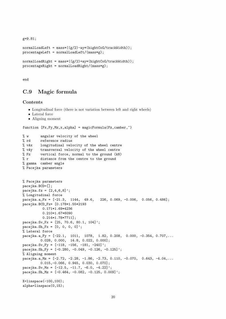
g=9.81;
normalLoadLeft = mass*((g/2)-ay*(hightCoG/trackWidth));
procentageLeft = normalLoadLeft/(mass*g);
normalLoadRight = mass*((g/2)+ay*(hightCoG/trackWidth));
procentageRight = normalLoadRight/(mass*g);
end
C.9 Magic formula
Contents
• Longitudinal force (there is not variation between left and right wheels)• Lateral force• Aligning moment
function [Fx,Fy,Mz,x,alpha] = magicFormula(Fz,camber,~)
% w angular velocity of the wheel
% rd reference radius
% vAx longitudinal velocity of the wheel centre
% vAy transversal velocity of the wheel centre
% Fz vertical force, normal to the ground (kN)
% r distance from the centre to the ground
% gamma camber angle
% Pacejka parameters
% Pacejka parameters
pacejka.BCD=[];
pacejka.fz = [2,4,6,8]’;
% Longitudinal force
pacejka.a_Fx = [-21.3, 1144, 49.6, 226, 0.069, -0.006, 0.056, 0.486];
pacejka.BCD_Fx= [0.178*1.55*2193
0.171*1.69*4236
0.210*1.67*6090
0.214*1.78*7711];
pacejka.Sv_Fx = [25, 70.6, 80.1, 104]’;
pacejka.Sh_Fx = [0, 0, 0, 0]’;
% Lateral force
pacejka.a_Fy = [-22.1, 1011, 1078, 1.82, 0.208, 0.000, -0.354, 0.707,...
0.028, 0.000, 14.8, 0.022, 0.000];
pacejka.Sv_Fy = [-118, -156, -181, -240]’;
pacejka.Sh_Fy = [-0.280, -0.049, -0.126, -0.125]’;
% Aligning moment
pacejka.a_Mz = [-2.72, -2.28, -1.86, -2.73, 0.110, -0.070, 0.643, -4.04,...
0.015,-0.066, 0.945, 0.030, 0.070];
pacejka.Sv_Mz = [-12.5, -11.7, -6.0, -4.22]’;
pacejka.Sh_Mz = [-0.464, -0.082, -0.125, 0.009]’;
X=linspace(-100,100);
alpha=linspace(0,15);
20

Longitudinal force (there is not variation between left and right wheels)
D = pacejka.a_Fx(1)*Fz^2+pacejka.a_Fx(2)*Fz;
C = 1.65;
% The BCD values for Fx are obtained by means of interpolation
BCD = (pacejka.a_Fx(3)*Fz^2+pacejka.a_Fx(4)*Fz)/(exp(pacejka.a_Fx(5)*Fz));
B = BCD/(C*D);
E = pacejka.a_Fx(6)*Fz^2+pacejka.a_Fx(7)*Fz+pacejka.a_Fx(8);
Sv = interpo2(pacejka.fz,pacejka.Sv_Fx,Fz);
Sh = interpo2(pacejka.fz,pacejka.Sh_Fy,Fz);
x=X+Sh;
Fx = D*sin(C*atan(B*x-E*(B*x-atan(B*x))))+Sv;
Lateral force
D = pacejka.a_Fy(1)*Fz^2+pacejka.a_Fy(2)*Fz;
C = 1.30;
BCD = pacejka.a_Fy(3)*sin(pacejka.a_Fy(4)*atan(pacejka.a_Fy(5)*Fz));
B = BCD/(C*D);
E = (pacejka.a_Fy(6)*Fz^2+pacejka.a_Fy(7)*Fz+pacejka.a_Fy(8))/(1-pacejka.a_Fy(13)*abs(camber));
% Sh = interpo2(pacejka.fz,pacejka.Sh_Fy,Fz)+pacejka.a_Fy(9)*camber;
% Sv = interpo2(pacejka.fz,pacejka.Sv_Fy,Fz)+(pacejka.a_Fy(10)*Fz^2+pacejka.a_Fy(11)*Fz)*camber;
xd = alpha; %Sh+alpha;
Fy = D*sin(C*atan(B*xd-E*(B*xd-atan(B*xd))));
Fy = Fy; %+ Sv;
Aligning moment
D = (pacejka.a_Mz(1)*Fz.^2+pacejka.a_Mz(2)*Fz);
C = 2.40;
BCD = (pacejka.a_Mz(3)*Fz^2+pacejka.a_Mz(4)*Fz)/(exp(pacejka.a_Mz(5)*Fz));
B = BCD/(C*D);
E = (pacejka.a_Mz(6)*Fz^2+pacejka.a_Mz(7)*Fz+pacejka.a_Mz(8))/(1-pacejka.a_Mz(13)*abs(camber));
% Sh = interpo2(pacejka.fz,pacejka.Sh_Mz,Fz)+pacejka.a_Mz(9)*camber;
% Sv = interpo2(pacejka.fz,pacejka.Sv_Mz,Fz)+(pacejka.a_Mz(10)*Fz^2+pacejka.a_Mz(11)*Fz)*camber;
xd = alpha; %Sh+alpha;
Mz = D*sin(C*atan(B*xd-E*(B*xd-atan(B*xd))));
Mz = Mz; %+ Sv;
C.10 Force in the rack
function f_rack=forceinrack(M,Force,h3,h4,h5,h6,h7,h8)
uw=(h4-h3)/norm(h4-h3); %steering axis
A=[ 1 0 0 -uw(1)
0 1 0 -uw(2)
0 0 1 -uw(3)
uw(1) uw(2) uw(3) 0
];
b=[ h3(1) h3(2) h3(3) dot(uw,h6)]’;
M1=A\b;
O_st=(M1(1:3))’;
% Point calculated as an intersection of axis 3-4 and a plane perpendicular and containing h6
r_steer_str= (O_st-h6);
u_steer=(h6-h7)/norm(h6-h7);
21

% chi1=zeros(100,3);
R_steer=zeros(100,3);
f_rack=zeros(1,100);
for i=1:100
% chi1(i,:)=-dot(M(i,:),uw)*uw-cross(Force(i,:),r_tireforce);
% R_steer(i,:)=-u_steer*norm(chi1(i,:))/(norm(r_steer_str)*norm(cross(u_steer,r_steer_str))/...
% (norm(u_steer)*norm(r_steer_str)));
% f_rack(i)=R_steer(i,2);
% dir=cross(u_steer,r_steer_str);
% R_steer(i,:)=[M(i,1)/dir(1) M(i,2)/dir(2) M(i,3)/dir(3)];
% f_rack(i)=R_steer(i,2);
R_steer=norm(M(i,:))/(sin(acos(dot(r_steer_str,u_steer)/norm(r_steer_str)))*norm(r_steer_str));
f_rack(i)=R_steer*u_steer(2);
end
C.11 interpo
function y = interpo2(X,Y,x)
n=length(X);
b=Y;
for j=2:n
for i=n:-1:j
b(i)=(b(i)-b(i-1))/(X(i)-X(i-j+1));
end
end
y=b(1)+b(2)*(x-X(1))+b(3)*(x-X(1))*(x-X(2))+b(4)*(x-X(1))*(x-X(2))*(x-X(3));
22
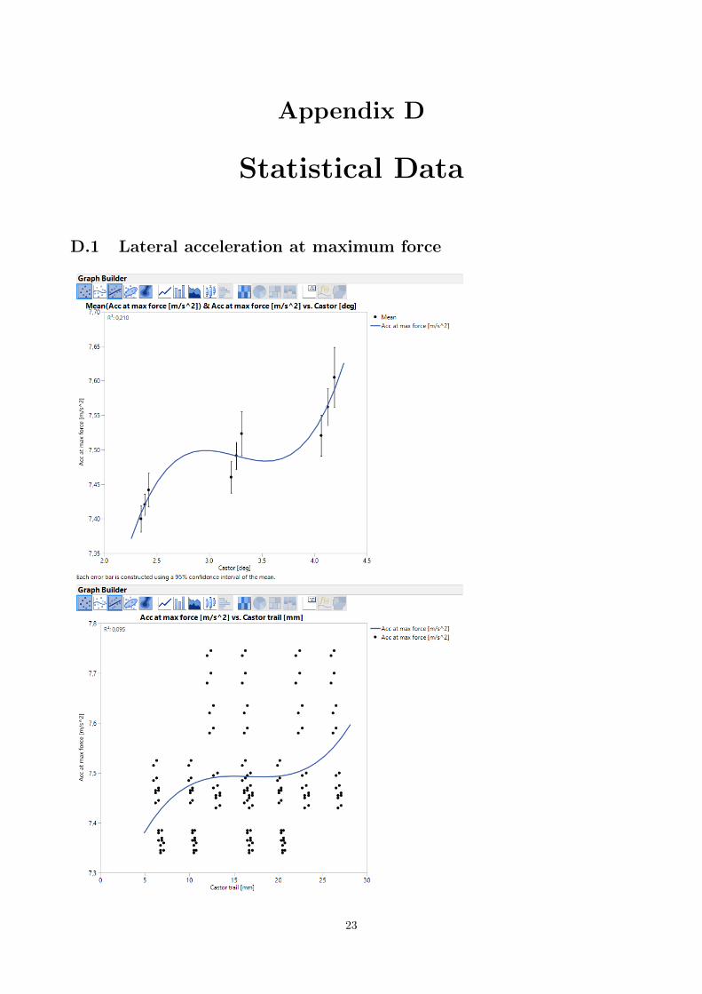
Appendix D
Statistical Data
D.1 Lateral acceleration at maximum force
23

24

25

26
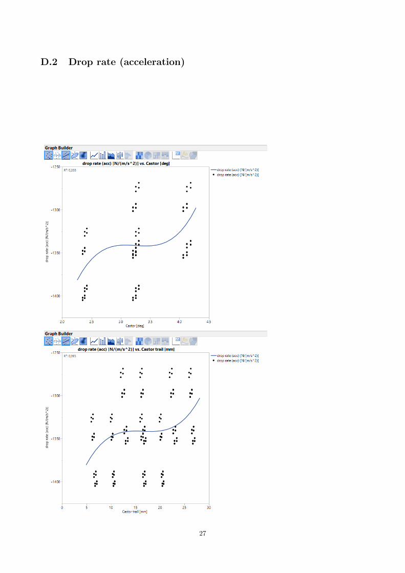
D.2 Drop rate (acceleration)
27

28

29

D.3 Drop rate (slip angel)
30
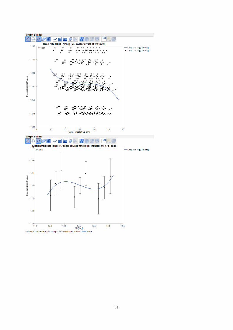
31
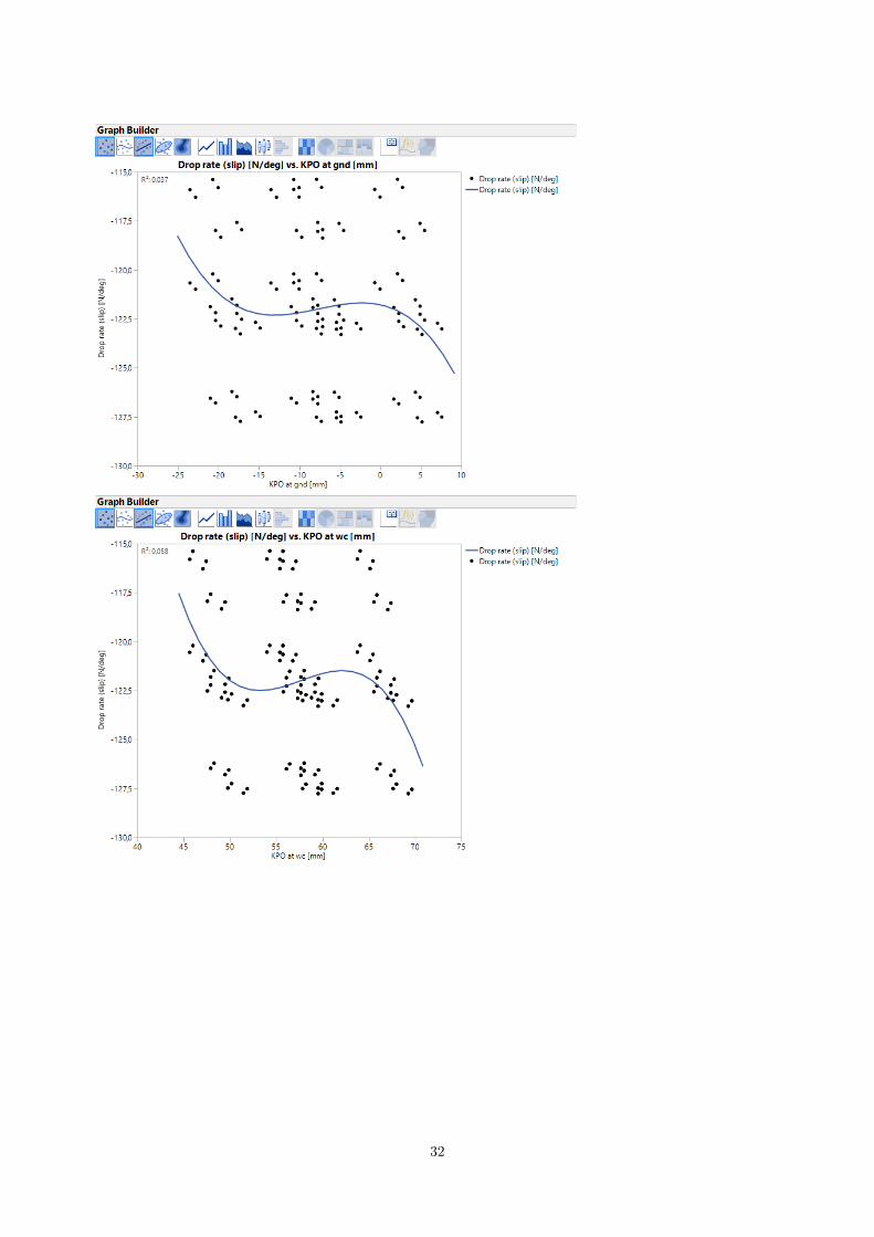
32
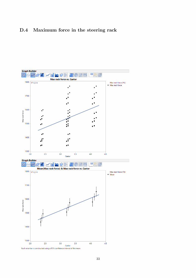
D.4 Maximum force in the steering rack
33

34

35

36

D.5 On-centre slip angle
37

38
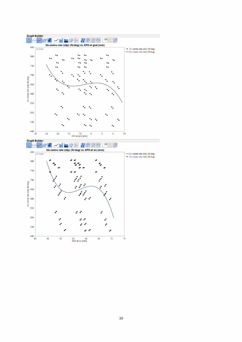
39

D.6 On-centre rate (acceleration)
40

41

42
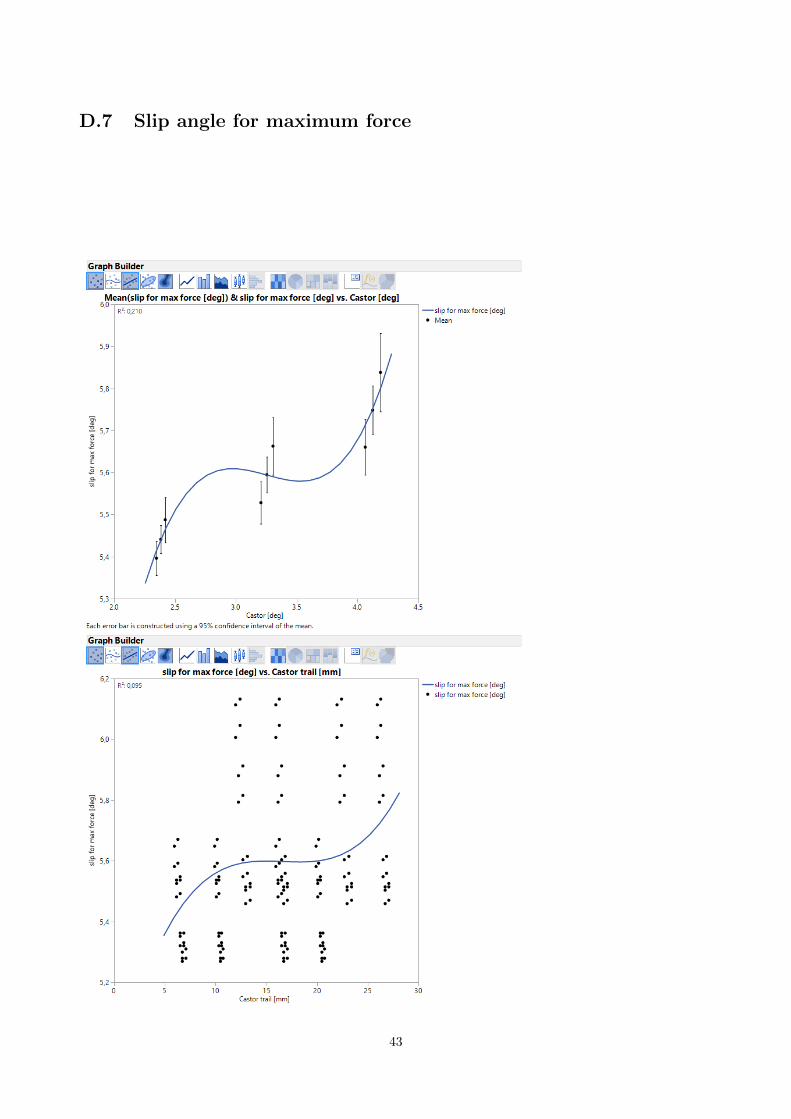
D.7 Slip angle for maximum force
43

44

45