learning-based route management in …cs.brown.edu/~mlittman/theses/russell.pdflearning-based route...

LEARNING-BASED ROUTE MANAGEMENT IN WIRELESSAD HOC NETWORKS

BY BRIAN RUSSELL

A dissertation submitted to the

Graduate School—New Brunswick

Rutgers, The State University of New Jersey

in partial fulfillment of the requirements

for the degree of

Doctor of Philosophy

Graduate Program in Computer Science

Written under the direction of

Michael Littman and Wade Trappe

and approved by

New Brunswick, New Jersey

October, 2008

c© 2008

Brian Russell

ALL RIGHTS RESERVED

ABSTRACT OF THE DISSERTATION

Learning-Based Route Management in Wireless Ad Hoc Networks

by Brian Russell

Dissertation Director: Michael Littman and Wade Trappe

The nodes in a wireless ad hoc network must act as routers in a self-configuring network

without infrastructure. An application running on nodes in the ad hoc network may require that

intermediate nodes act as routers, receiving and forwarding data packets to other nodes to over-

come limitations of noise, router congestion and limited transmission power. In existing routing

protocols, the “self-configuring” aspect of network construction hasgenerally been limited to

route selection using a shortest-path routing metric as a predictor of routing efficiency. This

limited, network-layer predictor fails to consider the effects of existing traffic on router loads

and fails to consider the effects of noise experienced at the MAC layer. Not all network topolo-

gies are suited to efficient routing using a shortest-path metric. The location of the nodes and

physical characteristics of the network environment can create topologies where shortest-path

routing overloads some routers and underutilizes others. Similarly, noise sources can under-

mine the quality of wireless links depending on the relative distance between thenoise sources

and the receiving nodes. This dissertation presents a cross-layer predictor that combines the

effects of noise and router congestion into a single time-based routing metric based on statis-

tical estimation from recent experience. Also presented is a new cross-layer, adaptive routing

protocol, called Warp-5, that not only uses the new routing metric to make better initial routing

decisions in a noisy or congested network, but can also adjust previously existing routes as new

routes or new noise sources are added to the network. Simulation results for Warp-5 are pre-

sented and compared to the existing shortest-path routing protocol AODV. The results show the

cross-layer approach of Warp-5 to be superior to shortest-path routing protocols for managing

router congestion and noise in wireless ad hoc networks.

ii

Dedication

This dissertation is dedicated to my wife,

Susan,

who never did get used to the mess.

And to

Irv

I came back, just like I promised.

iii

Table of Contents

Abstract . . . . . . . . . . . . . . . . . . . . . . . . . . . . . . . . . . . . . . . . . ii

Dedication . . . . . . . . . . . . . . . . . . . . . . . . . . . . . . . . . . . . . . . . iii

List of Tables . . . . . . . . . . . . . . . . . . . . . . . . . . . . . . . . . . . . . . viii

List of Figures . . . . . . . . . . . . . . . . . . . . . . . . . . . . . . . . . . . . . . ix

1. Introduction . . . . . . . . . . . . . . . . . . . . . . . . . . . . . . . . . . . . . 1

1.1. Wireless Ad Hoc Networks . . . . . . . . . . . . . . . . . . . . . . . . . . . . 1

1.2. Routing Protocols . . . . . . . . . . . . . . . . . . . . . . . . . . . . . . . . . 2

1.3. Coordinating Communication in Wireless Networks . . . . . . . . . . . . . . . 4

1.3.1. Basic Access Method . . . . . . . . . . . . . . . . . . . . . . . . . . . 5

1.3.2. RTS/CTS Protocol . . . . . . . . . . . . . . . . . . . . . . . . . . . . 6

1.4. Wireless Transmission Rates and Packet Forwarding Capacity . . . . .. . . . 7

1.5. Applications of Wireless Ad Hoc Networks . . . . . . . . . . . . . . . . . . . 9

1.5.1. Military Applications . . . . . . . . . . . . . . . . . . . . . . . . . . . 9

1.5.2. Industrial Applications . . . . . . . . . . . . . . . . . . . . . . . . . . 10

1.5.3. Wireless Ad Hoc Networks At Home . . . . . . . . . . . . . . . . . . 11

1.6. Thesis Statement . . . . . . . . . . . . . . . . . . . . . . . . . . . . . . . . . 12

1.7. Organization of Dissertation . . . . . . . . . . . . . . . . . . . . . . . . . . . 13

2. Previous Work . . . . . . . . . . . . . . . . . . . . . . . . . . . . . . . . . . . 14

2.1. Transmission Rate Selection . . . . . . . . . . . . . . . . . . . . . . . . . . . 16

2.1.1. Automatic Rate Fallback (ARF) . . . . . . . . . . . . . . . . . . . . . 17

2.1.2. Receiver-Based AutoRate (RBAR) . . . . . . . . . . . . . . . . . . . . 17

2.1.3. Adaptive Automatic Rate Fallback (AARF) . . . . . . . . . . . . . . . 18

iv

2.1.4. SampleRate . . . . . . . . . . . . . . . . . . . . . . . . . . . . . . . . 18

2.1.5. Discussion . . . . . . . . . . . . . . . . . . . . . . . . . . . . . . . . 19

2.2. Routing Protocols For Wireless Ad Hoc Networks . . . . . . . . . . . . . . .. 19

2.2.1. Destination-Sequenced Distance Vector (DSDV) Routing Protocol .. . 20

2.2.2. Ad-hoc On-Demand Distance Vector (AODV) Routing Protocol . . . .21

2.2.3. Dynamic Source Routing (DSR) Protocol . . . . . . . . . . . . . . . . 22

2.2.4. Optimized Link State Routing (OLSR) Protocol . . . . . . . . . . . . . 23

2.2.5. Zone Routing Protocol (ZRP) . . . . . . . . . . . . . . . . . . . . . . 23

2.2.6. Sharp Hybrid Adaptive Routing Protocol (SHARP) . . . . . . . . . . .24

2.2.7. Discussion and Other Previous Work . . . . . . . . . . . . . . . . . . 24

2.3. Machine-Learning Based Routing Protocols . . . . . . . . . . . . . . . . .. . 25

2.3.1. Q-Routing . . . . . . . . . . . . . . . . . . . . . . . . . . . . . . . . 27

2.3.2. Predictive Q-Routing . . . . . . . . . . . . . . . . . . . . . . . . . . . 28

2.3.3. Dual Reinforcement Q-Routing . . . . . . . . . . . . . . . . . . . . . 29

2.3.4. Policy-Gradient Q-Routing . . . . . . . . . . . . . . . . . . . . . . . . 30

2.3.5. Gradient Ascent Q-Routing . . . . . . . . . . . . . . . . . . . . . . . 31

2.3.6. Least Squares Policy Iteration Q-Routing . . . . . . . . . . . . . . . . 31

2.3.7. CMAC-Based Q-Routing . . . . . . . . . . . . . . . . . . . . . . . . . 32

2.3.8. Ant-Based Q-Routing . . . . . . . . . . . . . . . . . . . . . . . . . . 33

2.3.9. Q-Routing in Mobilized Ad hoc Networks . . . . . . . . . . . . . . . . 34

2.3.10. Discussion . . . . . . . . . . . . . . . . . . . . . . . . . . . . . . . . 35

3. Mathematical Models For Communication and Routing . . . . . . . . . . . . . 38

3.1. A Mathematical Model For Noise And Packet Loss . . . . . . . . . . . . . .. 38

3.2. A Time-Based Routing Metric . . . . . . . . . . . . . . . . . . . . . . . . . . 41

3.3. Calibrating Noise Sources for Specific Packet Loss Effects . . . . .. . . . . . 43

4. The Warp-5 Routing Algorithm . . . . . . . . . . . . . . . . . . . . . . . . . . 48

4.1. Route Requests . . . . . . . . . . . . . . . . . . . . . . . . . . . . . . . . . . 49

4.2. Route Construction . . . . . . . . . . . . . . . . . . . . . . . . . . . . . . . . 50

v

4.2.1. Route Construction Example . . . . . . . . . . . . . . . . . . . . . . . 52

4.3. Route Table Management in Routers . . . . . . . . . . . . . . . . . . . . . . . 53

4.4. Route Improvement and Detangling . . . . . . . . . . . . . . . . . . . . . . . 54

4.4.1. Route Detangling Example . . . . . . . . . . . . . . . . . . . . . . . . 56

4.4.2. Discussion . . . . . . . . . . . . . . . . . . . . . . . . . . . . . . . . 64

5. Machine Learning in Warp-5 . . . . . . . . . . . . . . . . . . . . . . . . . . . . 65

5.1. Selecting Link-level Transmission Rates . . . . . . . . . . . . . . . . . . . . .68

5.2. Estimating Probability of Unicast Failure . . . . . . . . . . . . . . . . . . . . 69

5.3. Learning Data Packet Arrival Rates . . . . . . . . . . . . . . . . . . . . .. . . 71

5.4. Estimating Time For Route Stabilization . . . . . . . . . . . . . . . . . . . . . 72

6. Noise and Congestion Simulations. . . . . . . . . . . . . . . . . . . . . . . . . 76

6.1. Simulation Environment . . . . . . . . . . . . . . . . . . . . . . . . . . . . . 77

6.2. Scientific Properties For Investigation . . . . . . . . . . . . . . . . . . . . . .79

6.2.1. Preventing Data Packet Loss Due To Router Congestion . . . . . . . .81

6.2.2. Responding to Router Congestion To Prevent Data Packet Loss . .. . 82

6.2.3. Preventing Data Packet Loss Due To Noise . . . . . . . . . . . . . . . 84

6.2.4. Responding To Noise To Minimize Data Packet Loss . . . . . . . . . . 86

6.3. Experimental Scenarios . . . . . . . . . . . . . . . . . . . . . . . . . . . . . . 87


6.3.2. Responding To Router Congestion To Minimize Data Packet Loss . . . 89



6.4. Simulation Results and Discussion . . . . . . . . . . . . . . . . . . . . . . . . 92


6.4.2. Responding To Router Congestion To Minimize Data Packet Loss . . . 98



6.5. Summary and Key Findings . . . . . . . . . . . . . . . . . . . . . . . . . . . 111

vi

7. Current Status and Future Work . . . . . . . . . . . . . . . . . . . . . . . . . 114

7.1. Detecting Link Failure . . . . . . . . . . . . . . . . . . . . . . . . . . . . . . 115

7.2. Mobile Ad Hoc Networks . . . . . . . . . . . . . . . . . . . . . . . . . . . . . 117

7.3. Quality Of Service . . . . . . . . . . . . . . . . . . . . . . . . . . . . . . . . 118

7.4. Extensions To The Detangling Algorithm . . . . . . . . . . . . . . . . . . . . 119

7.5. Conclusion . . . . . . . . . . . . . . . . . . . . . . . . . . . . . . . . . . . . 120

References. . . . . . . . . . . . . . . . . . . . . . . . . . . . . . . . . . . . . . . . 121

vii

List of Tables

1.1. Maximum packet forwarding rate (in packets per second) for 802.11 a/b/g

transmission rates for packet sizes 50, 100, 500, 100 and 1500 bytes.. . . . . . 8

viii

List of Figures

4.1. Topology for Route Construction Example With Links Between Adjacent Nodes. 51

4.2. The first route request is a route from Node 3 to Node 4, called the 3→4 route.

In a topology with no pre-existing routes, Warp-5 simply finds the shortest path,

as shown in the right side topology. Routers in the network have seen the RREP

packets for the 3→4 route and know that the 3→4 route is the first route created. 57

4.3. The second route request is a 1→6 route. The nodes on the 3→4 route have

established traffic, so Warp-5 finds a 1→6 route that avoids nodes used by

the previous route. The 1→6 and 3→4 routes do not overlap, no routers are

overloaded, so no router takes any corrective action. Routers in the network

know that 1→6 is the second route created. The right side topology shows the

least expensive 2→5 route, which overlaps the 3→4 route at nodes 3, 9, 15, 16,

17, 10 and 4. Routers in the network know that 2→5 is the third route created.

Given the existing 3→4 and 1→6 routes, it is impossible to create a 2→5 route

without overloading some router in the network. . . . . . . . . . . . . . . . . . 57

4.4. The left side topology shows Node 3 is overloaded as both a source of traffic for

the 3→4 route and an intermediate node for the 2→5 route. In response to the

overload, Node 3 modifies the 2→5 route. The modified 2→5 route will ignore

the other routes in the network. The right side topology shows the modified

2→5 route. By ignoring the other routes, the modified 2→5 route is a shortest

path between Node 2 and Node 5. . . . . . . . . . . . . . . . . . . . . . . . . 58

4.5. Node 8 responds to overload by modifying the 1→6 route. The modification

considers only the 2→5 route. The modified 1→6 route in the left side topology

now avoids the 2→5 route. . . . . . . . . . . . . . . . . . . . . . . . . . . . . 58

ix

4.6. Node 16 is overloaded and responds by modifying the 3→4 route. The mod-

ification considers the 2→5 and 1→6 routes. The 3→4 route could not be

improved under current circumstances and is shown unchanged in the left side

topology. . . . . . . . . . . . . . . . . . . . . . . . . . . . . . . . . . . . . . 59

4.7. Node 16 is still overloaded. Node 16 changes the shared routeList to(3→4,2→5,1→6)

and modifies the 1→6 route, ignoring all other routes. The resulting shortest-

path modification is actually worse. . . . . . . . . . . . . . . . . . . . . . . . 59

4.8. Node 10 is overloaded and responds by modifying the 2→5 route. The modifi-

cation considers only the 1→6 route and ignores the 3→4 route. The resulting

modification is not an improvement. . . . . . . . . . . . . . . . . . . . . . . . 59

4.9. Node 10 is still overloaded and responds by modifying the 3→4 route. The

modification considers the 2→5 and 1→6 routes. The 3→4 route could not be

improved under current circumstances and is shown unchanged in the left side

topology. . . . . . . . . . . . . . . . . . . . . . . . . . . . . . . . . . . . . . 60

4.10. Node 4 is overloaded. Node 4 changes the shared routeList to (2→5,3→4,1→6)


path modification is not an improvement. . . . . . . . . . . . . . . . . . . . . 60

4.11. Node 2 is overloaded and responds by modifying the 3→4 route. The modi-

fication considers only the 1→6 route. Note that the 3→4 route was selected

from the routeList as the next route to modify and does not directly affectNode

2. No change results from this modification. . . . . . . . . . . . . . . . . . . . 61


modification considers the 1→6 and 3→4 routes. The modified route is shown

in the left side topology. . . . . . . . . . . . . . . . . . . . . . . . . . . . . . . 61

4.13. Node 2 is still overloaded. Node 2 changes the shared routeList to (1→6,3→4,2→5)



4.14. Node 2 is still overloaded and responds by modifying the 3→4 route. The mod-

ification considers only the 2→5 route. The 3→4 route could not be improved

under current circumstances and is shown unchanged in the left side topology. . 62

x

4.15. Node 2 is still overloaded and responds by modifying the 1→6 route. The mod-

ification considers the 2→5 and 3→4 routes. The modification is premature,

and the modified route does not change significantly. . . . . . . . . . . . . . . 62

4.16. Node 2 is still overloaded. Node 2 changes the shared routeList to (1→6,2→5,3→4)




modification considers only the 3→4 route. The resulting modification is an

improvement. . . . . . . . . . . . . . . . . . . . . . . . . . . . . . . . . . . . 63

4.18. Node 15 is overloaded and responds by modifying the 1→6 route. The mod-

ification considers the 2→5 and 3→4 routes. The result is a stable detangled

network with no overloaded nodes. . . . . . . . . . . . . . . . . . . . . . . . . 63

5.1. Warp-5 Estimating Probability of Unicast Failure. . . . . . . . . . . . . . . . .71

5.2. Warp-5 Learning Data Packet Arrival Rates. . . . . . . . . . . . . . .. . . . . 72

5.3. Calculation of Gaussian values . . . . . . . . . . . . . . . . . . . . . . . . . . 75

5.4. Warp-5 Expectation Management Algorithm. . . . . . . . . . . . . . . . . . . 75

6.1. Castle Topology for Congestion Problems . . . . . . . . . . . . . . . . . . . .77

6.2. Square Topology With Active Noise Sources . . . . . . . . . . . . . . . . .. . 78

6.3. Preventable Router Congestion. . . . . . . . . . . . . . . . . . . . . . . . . .81

6.4. Correctable Router Congestion. . . . . . . . . . . . . . . . . . . . . . . . . .. 83

6.5. Square Topology With Poorly Chosen Routes . . . . . . . . . . . . . . . . .. 85

6.6. Square Topology Before Noise Source Activation . . . . . . . . . . . .. . . . 86

6.7. AODV and Warp-5 Data Packet Arrival Rates For Low Offered Load Simulations 93

6.8. AODV and Warp-5 Data Packet Arrival Rates For Medium OfferedLoad Sim-

ulations . . . . . . . . . . . . . . . . . . . . . . . . . . . . . . . . . . . . . . 95

6.9. AODV and Warp-5 Data Packet Arrival Rates For High Offered Load Simulations 96

6.10. Preventing Router Congestion. . . . . . . . . . . . . . . . . . . . . . . . . .. 97

6.11. AODV and Warp-5 Data Packet Arrival Rates For Router Congestion Problems

(single-radio nodes). . . . . . . . . . . . . . . . . . . . . . . . . . . . . . . . 98

xi

6.12. AODV and Warp-5 Data Packet Arrival Rates For Router Congestion Problems

(dual-radio nodes). . . . . . . . . . . . . . . . . . . . . . . . . . . . . . . . . 100

6.13. Adjusting to Router Congestion. . . . . . . . . . . . . . . . . . . . . . . . . . 101

6.14. AODV and Warp-5 Data Packet Arrival Rates For 54 Mbits/sec in a noisy en-

vironment. . . . . . . . . . . . . . . . . . . . . . . . . . . . . . . . . . . . . . 103

6.15. AODV and Warp-5 Data Packet Arrival Rates For 6 Mbits/sec in a noisy envi-

ronment. . . . . . . . . . . . . . . . . . . . . . . . . . . . . . . . . . . . . . . 104

6.16. Preventing Data Packet Loss In Noisy Environment . . . . . . . . . . .. . . . 106

6.17. AODV and Warp-5 Data Packet Arrival Rates For 54 Mbits/sec Response to

Noise. . . . . . . . . . . . . . . . . . . . . . . . . . . . . . . . . . . . . . . . 108

6.18. AODV and Warp-5 Data Packet Arrival Rates For 6 Mbits/sec Response to Noise.109

6.19. Adjusting to Noise. . . . . . . . . . . . . . . . . . . . . . . . . . . . . . . . . 110

xii

1

Chapter 1

Introduction

Establishing and maintaining routes in a wireless ad hoc network is an essentialcomponent

to supporting communications across a broad geographical area when individual nodes have

limited communication range. Although many wireless routing protocols exist, the problem of

supporting efficient and effective communication by establishing appropriate routes is a chal-

lenging task for which there is no completely adequate protocol in the literature. This disser-

tation seeks to address this problem by applying machine-learning techniques to wireless ad

hoc routing. In particular, this dissertation shows that machine learning is feasible and useful

in managing noise and router congestion in wireless ad hoc networks to improve distributed

application throughput.

1.1 Wireless Ad Hoc Networks

A wireless ad hoc network is a collection of nodes exchanging information through radio or

infrared wireless adapters. Such a network functions without an established infrastructure. In

infrastructure-based wireless networks, there is no direct peer-to-peer communication between

nodes; all communication between nodes is managed by the network infrastructure. One exam-

ple of an infrastructure-based network is the wireless local area network, or wireless LAN. The

infrastructure of a wireless LAN consists of access points connected bythe Internet. Wireless

nodes communicate with the access points and the access points provide networking function-

ality to the wireless nodes. Another example of an infrastructure-based network is the cellular

system. In cellular systems, a geographical area is divided intocells, each with abase station

at the center of the cell. The base stations are connected to a backbone wired network. The

base stations and the backbone wired network form the infrastructure for the cellular system.

Wireless nodes communicate with the base stations, and the base stations in combination with

2

the backbone wired network perform the networking functions and direct communication to

other wireless nodes.

Nodes in an ad hoc wireless network, on the other hand, communicate with each other on a

peer-to-peer basis, and the networking functions are distributed among the nodes in the ad hoc

network. Without an infrastructure, the nodes in a wireless ad hoc network must act as routers

in a self-configuring network. A distributed application running on nodes inthe wireless ad hoc

network, such as a video feed between two parties separated by a large distance, may require

that intermediate nodes act as routers, receiving and forwarding data packets to other nodes as

needed.

The use of radio or infrared adapters as links in wireless ad hoc networks introduces char-

acteristics that are not present in wired networks. Given a powerful enough transmission, any

two nodes in a wireless ad hoc network can communicate directly. However, for a fixed trans-

mit power, the received signal power decreases rapidly as the distancebetween sender node

and receiver node increases. When sender and receiver nodes are separated by a large dis-

tance, the high-powered transmissions required for direct wireless communication can cause

interference in other links in the network, degrading their performance or breaking the other

links altogether. Using intermediate nodes with limited communication range as forwarding

relays can reduce the sum of transmit power at the source and intermediatenodes needed for

source-to-destination communication. Routing using intermediate nodes allows geographically

dispersed nodes to communicate with less power expenditure and less interference with other

links in the wireless ad hoc network.

1.2 Routing Protocols

The need for routing protocols in wireless ad hoc networks is prompted by the limited commu-

nication range used by radio and infrared wireless adapters. Limitations onthe direct commu-

nication range between nodes and the need for many nodes to cover an area much larger than

the limited direct communication range means that nodes in an ad hoc network have to act as

intermediaries, forwarding information to destination nodes that could not bereached directly

3

by the original sending nodes. The purpose of a routing protocol is to find a sequence of inter-

mediate nodes from a source node to a destination node. A sequence of nodes from source to

destination is called aroute.

Previous routing protocols such as DSDV use frequent system-wide broadcasts of global

routing information to maintain current connectivity between all nodes in the adhoc net-

work [46]. A complete global picture held by all nodes almost always exceeds the needs of

the application in the ad hoc network. Further, with each node having to sendand maintain

routing information for the entire network, the amount of routing overhead grows in proportion

to the square of the number of nodes in the network, which limits the scalability of the approach.

Later approaches to route construction, such as AODV [47] and DSR [30], employed an on-

demand approach in response to scalability issues, where routes are constructed as needed, and

eliminated the need for maintaining and broadcasting global connectivity information. Both

AODV and DSR are distance-vector protocols [36] that seek to find the best routes from the

source to a destination, where “best route” is generally defined to be the route with the fewest

intermediate nodes (“hops”) between source and destination.

Each route consumes some of the finite forwarding capacity of the routers ituses as packets

are sent from source to destination, reducing the speed at which all traffic moves through the

routers. Using the minimal hop count as a routing metric ignores the effects ofexisting routes

on router forwarding. The same metric also does not consider the quality oflinks connecting

neighbors, which may be affected by packet collisions on crowded links or noise. Congested

routers drop packets, reducing the number of application data packets that reach their intended

destination. Transmission of packets over lossy links forces either retransmission of packets

with concomitant loss of time, or loss of data packets altogether. In order to support better

communication, what is needed is a routing metric that considers router loadingand link qual-

ity. Such a routing metric would make it possible to avoid bottlenecks caused by forcing too

many routes through too few routers and increase overall application datathroughput.

4

1.3 Coordinating Communication in Wireless Networks

This section discusses the mechanics of how wireless nodes share a singlecommunication

channel for data packet transfer in wireless networks.

Routers in wired networks have multiple adapters, one for each neighboring node. A wired

router receives a data packet for a remote destination through one adapter, extracts the final

destination of the data packet from the IP address in the packet network header, consults a

routing table to determine the appropriate outgoing adapter and then transmits thedata packet

through the outgoing adapter. With the proper internal switching fabric, a wired router can

receive and forward data packets through different adapters simultaneously.

Routers in wireless networks forward data packets in a different fashion. The wireless

router has a single adapter for all incoming and outgoing data packet transmissions. All wire-

less routers in the wireless network exchange data packets through the same communication

channel. An incoming data packet is received on the adapter, which determines that the re-

ceiving neighbor is the intended intermediate destination from the destination address in the

Medium Access Control (MAC) header. The wireless router then extracts the final destination

of the data packet from the IP address in the packet network header, and consults a routing table

to determine the appropriate next hop for the packet and then transmits the data packet through

the wireless adapter to the next hop node.

The difference between the router in the wired network and the router in thewireless net-

work is while the router in the wired network can receive and forward datapackets through each

of its multiple adapters simultaneously, the router in the wireless network can onlyreceive or

transmit one data packet at a time through a single wireless adapter. Worse still, the data packets

in the wireless network are communicated through omnidirectional transmissionsreceived by

all nodes within communication range. Multiple overlapping transmissions render themselves

unintelligible to the receivers, so the nodes in a wireless network have to cooperatively coordi-

nate which node can transmit and when that node can transmit on the communication channel

shared by all the nodes in the wireless network. The coordination of communication in 802.11

wireless networks is performed by the 802.11 Distributed Coordination Function (DCF), orig-

inally defined in the IEEE 802.11 standard [24]. The DCF uses carrier sensing multiple access

5

with collision avoidance (CSMA/CA). There are two protocols in the DCF: the basic access

method and the RTS/CTS protocol. This dissertation focuses on wireless ad hoc networks built

on the 802.11 MAC layer.

1.3.1 Basic Access Method

A node with a packet to transmit must monitor the communication medium to ensure thatit

has been idle for a period of at least DIFS (DCF InterFrame Space). Ifthe medium has been

idle for DIFS or longer, the node is free to transmit the packet immediately. If the medium

is not idle or has been idle for a period less than DIFS, the node must wait untilthe medium

has been idle for at least DIFS time. The node then selects a discrete random backoff counter

before transmitting the packet. The underlying assumption here is that there may be multiple

nodes in the same area waiting to transmit. Once the nodes detect the medium becoming idle

after a transmission, independently selected random backoff period will minimize the chance

of overlapping transmissions. The backoff counter is uniformly selected from a contention

window value initially set by a value specific to the individual PHY layer implementation.

The backoff counter is decremented at the end of a discrete time slot if the communication

medium is still idle. The duration of the slot is the time required for the node to sense the

medium to determine if it is still idle. The backoff counter is not decremented when the node

determines that the medium is busy. When the backoff counter is decrementedto zero, the node

transmits the packet.

In this dissertation, a packet transmission intended for a single receiver iscalled aunicast

1. Unicast packets must be acknowledged by the receiver. To do so, thereceiver sends a

small (14 byte) acknowledgement (ACK) packet to the sender after an interval SIFS (Short

InterFrame Space), which must be smaller than DIFS to ensure that the ACK packet can be

transmitted before another node attempts to transmit a packet. If the sending node receives the

ACK packet, then the unicast is considered successful and no furtheraction is taken by the

sender for that packet. If the sender does not receive an ACK packet within a fixed timeout

interval, it doubles the value of the contention window and selects a new random backoff value,

1The termunicastalso refers to any communication from a source to a single receiver.

6

at the end of which, it will retransmit the unicast packet. This retransmissionprocedure is

repeated, doubling the contention window each time until either the sending node receives an

ACK packet from the receiver or the contention window reaches some maximum size specific

to the individual PHY layer implementation. In the latter event, the packet is dropped and the

unicast is considered a failure.

The wireless network simulations documented in Chapter 6 use a simulation of the 802.11

MAC layer based on Direct Sequence Spread Spectrum (DSSS) with a SIFS of 10 microsec-

onds, a DIFS of 50 microseconds, an initial contention window size of 32 and a maximum

contention window size of 1024. The slot size used for random backoffis 20 microseconds.

The timeout for ACK packet return is 300 microseconds.

The random binary exponential backoff mechanism described in the 802.11 standard is an

effective means of managing contention for the communication medium [3]. Thealgorithm

self-adjusts to small or large numbers of contending nodes in a few steps. The same algorithm

is less applicable for responding to noise. While some sort of distributed randomized waiting is

an effective means of sharing the communication medium, the same waiting response to noise

when there is little contention leads to stretches where no node is transmitting, even when there

are multiple nodes with packets to transmit. A more effective response to noise isthe immediate

retransmission of the failed unicast to increase the likelihood of correct reception of the packet.

1.3.2 RTS/CTS Protocol

A node with a packet to transmit must monitor the communication medium to ensure thatis

has been idle for at least DIFS time, and after that choose a random backoff counter, just as

it would for the basic access method. When the backoff counter is decremented to zero, the

transmitting node sends a 20 byte Request To Send (RTS) packet to the receiver. The RTS

packet contains the duration that the sender wants for exclusive access to the communication

medium in microseconds. The duration in the RTS packet is the time required to send a data

packet, a clear to send (CTS) packet, and an ACK packet plus three SIFS intervals. The receiver

of the RTS packet responds to the RTS packet after a SIFS interval by transmitting a CTS packet

containing a duration to the sender. The duration in the CTS packet is the time required to send

the data packet, and an ACK packet plus two SIFS intervals, in microseconds. When the sender

7

receives the CTS packet, it transmits its packet after a SIFS interval.

Any node in communication range of the RTS and CTS transmissions will also receive the

RTS or CTS packets. Nodes other than the receiver that overhear onlythe RTS packet will

not transmit during the duration specified in the RTS packet. Nodes other than the sender or

receiver that overhear the CTS packet will not transmit during the duration specified in the CTS

packet.

The RTS/CTS protocol is an effective means of dealing withhidden nodes, where there may

be other nodes within communication range of the receiver, but not the sender. The RTS/CTS

protocol also reduces the chances of packet collisions, since the only potential for collision is

during the transmission of the short RTS packet.

1.4 Wireless Transmission Rates and Packet Forwarding Capacity

There are three different 802.11 PHY layers currently available, designated 802.11b, 802.11a

and 802.11g. Each layer offers multiple transmission rates. The maximum packet transfer

capacity for each transmission rate for all three 802.11 PHY layers is shown in Table 1.1. The

first and second column identify a specific PHY layer and transmission rate,the transmission

rate expressed in megabits per second. The next five columns shown different packet sizes, with

50 bytes being considered a small packet and 1500 bytes a large packet.Individual entries under

each of the packet size columns is the maximum number of packets per secondthat can be sent

for that PHY/transmission rate combination for that packet size given the overhead required by

the DCF for that PHY implementation. The individual rates for maximum number ofpackets

per second transfer are based on a 50 microsecond DIFS, an initial contention window size of

32, a maximum contention window size of 1024, a 20 microsecond slot size andan average

random backoff time of 320 microseconds.

The fastest 802.11b transmission rate is eleven times faster than the slowest 802.11b trans-

mission rate. However, the communication medium coordination overhead imposed by the

DCF reduces the potential packet transfer rate for the 11 Mbits/sec transmission rate to less

than twice the potential packet transfer rate for the 1 Mbits/sec transmission rate for 50 byte

packets and a little over eight-fold for 1500 byte packets. The increase in bandwidth for packets

8

Protocol Rate 50 bytes 100 bytes 500 bytes 1000 bytes 1500 bytes802.11b 1 Mbits/sec 1265.80 840.33 227.79 119.19 80.71802.11b 2 Mbits/sec 1694.90 1265.80 418.41 227.79 156.49802.11b 5.5 Mbits/sec 2161.10 1867.60 895.04 542.14 388.83802.11b 11 Mbits/sec 2345.40 2161.10 1326.90 895.04 675.26802.11a/g 6 Mbits/sec 2189.78 1910.80 946.40 580.27 418.41802.11a/g 9 Mbits/sec 2301.79 2088.20 1198.40 781.93 580.27802.11a/g 12 Mbits/sec 2362.20 2189.78 1382.59 946.37 719.40802.11a/g 18 Mbits/sec 2425.88 2301.79 1633.39 1198.40 946.37802.11a/g 24 Mbits/sec 2459.02 2362.20 1796.41 1382.49 1123.60802.11a/g 36 Mbits/sec 2493.07 2425.80 1995.57 1633.39 1382.49802.11a/g 48 Mbits/sec 2510.46 2459.02 2112.68 1796.41 1562.50802.11a/g 54 Mbits/sec 2516.31 2470.27 2154.83 1858.22 1633.39

Table 1.1: Maximum packet forwarding rate (in packets per second) for802.11 a/b/g transmis-sion rates for packet sizes 50, 100, 500, 100 and 1500 bytes.

of a particular size is not directly proportional to the increase in transmissionrate due to the

overhead imposed by the 802.11 DCF.

The fastest 802.11a transmission rate is nine times faster than the slowest 802.11a transmis-

sion rate. Increasing the transmission rate for 50 byte packets from 6 Mbits/sec to 54 Mbits/sec

results in only a 14.91 percent increase in data transfer speed, again due to overhead imposed

by the 802.11 DCF. Increasing the transmission rate for 1500 byte packetsfrom 6 Mbits/sec to

54 Mbits/sec results in a 290.38 percent increase in data transfer speed,much greater than the

increase gained for 50 byte packets. Although the contention control overhead imposed by the

802.11 DCF does reduce data transfer rates regardless of transmission rate, larger packets get

greater benefits from faster transmission rates than smaller packets.

The slowest 802.11b wireless transmission rate provides a link capacity of approximately

0.6 Mbits/sec for 1500 byte packets after correcting for overhead required by the 802.11 Dis-

tributed Coordination Function. The fastest 802.11g wireless transmission rate provides a link

capacity of approximately 20 Mbits/sec for 1500 byte packets after correcting for DCF over-

head. In contrast, a wired 802.3z Ethernet link has a capacity of 1 gigabit/sec and a wired

802.3ae Ethernet link has a capacity of 10 gigabits/sec [15], [25]. The 10 gigabit 802.3ae

wired Ethernet link provides 500 times the capacity of the fastest 802.11 wireless link. The

magnitude of the disparity between wired and wireless links, and the wide variety of current

and developing applications for wireless ad hoc networks in different areas underscores the

9

importance of using the limited bandwidth of wireless links effectively. The effective use of

wireless links in ad hoc networks is the motivation for the research in this dissertation.

1.5 Applications of Wireless Ad Hoc Networks

The self-configuring capabilities of wireless ad hoc networks coupled withthe lack of costly

infrastructure, makes them appealing for many applications in a variety of circumstances. The

success of wireless ad hoc networks comes from their flexibility, making themuseful for new

circumstances as the need arises. The lack of infrastructure and ease of reconfigurability must

be balanced against the performance penalties inherent to wireless ad hoc networks including

wireless communication, multi-hop routing and distributed routing control. The very flexibility

means that research into wireless ad hoc networks must balance flexibility ofdesign against

varying application needs. A network designed to meet a wide variety of circumstances may

not be able to meet stringent performance requirements for some distributedapplications. Con-

versely, a network designed to meet specific stringent requirements may beless useful in gen-

eral. The ideal wireless ad hoc network design would be flexible enough tosupport a variety of

distributed applications while being capable of meeting high performance requirements when

needed.

This section describes some of the common applications for wireless ad hoc networks.

There are distributed applications on the battlefield, in industry and in the home.

1.5.1 Military Applications

The inherent lack of infrastructure makes wireless ad hoc networks desirable for military sit-

uations where networks must be dropped (literally) into remote and often hostile areas where

network infrastructure is nonexistent and cannot be developed. Suchnetworks have to be built,

configured and torn down quickly. Military scenarios require sensor networks and intelligence

gathering mechanisms placed close to potential targets. A sensor network consists of small

nodes with sensing, computation and wireless networking capabilities. The nodes in the sensor

network could contain passive optical, electromagnetic, audio, chemical, orbiological sensors.

Optical sensors could be used to coordinate unmanned aircraft in flight, or provide networked

10

navigation on the ground by routing vehicles effectively through complex terrain and constantly

changing hazards. Electromagnetic sensors could be used to monitor hostilecommunications

as well as detect military hazards like land mines and active radar signals. Chemical and bio-

logical sensors can be used to monitor the presence of chemical and biological warfare agents

to provide vital information necessary to the planning of troop movement on thebattlefield.

The potential threat to the network devices is quite high, and the network mustbe robust to

hazardous conditions and loss of nodes with minimal human intervention.

The United States military plans to use networked communication on a grand scale.The

Department of Defense wants to assign a unique IP address to every piece of equipment and ev-

ery soldier on the electronic battlefield [53]. The Defense Advanced Research Project Agency

(DARPA) project GLOMO (GLObal MObile information system), intended to develop high-

speed metropolitan area networks for multimedia communication, has met with limited suc-

cess [40], [51].

1.5.2 Industrial Applications

Networking without the overhead of infrastructure installation and maintenance costs makes

wireless ad hoc networks attractive in the industrial world. Wireless ad hocnetworks can

support distributed control applications with sensors and actuators connected with wireless

networks. Wireless sensor networks can be deployed in mines, nuclear power plants and other

hazardous industrial environments. In less dangerous industrial environments, analog control

systems for heating, ventilation and cooling (HVAC) systems can be replacedwith more energy

efficient digital controls that communicate through wireless ad hoc networks. Similarly, large-

scale lighting systems and motor controls could also be made more energy efficient by replacing

the analog control systems with digital controls that communicate through wireless ad hoc

networks [21].

Wireless ad hoc networks can be used to coordinate automated vehicles in industrial envi-

ronments and the control of industrial and manufacturing processes. Wireless ad hoc networks

could provide the coordination, sensing and control of industrial processes while the lack of in-

frastructure provides reconfigurability and scalability on an economical basis as the industrial

environment changes and expands.

11

1.5.3 Wireless Ad Hoc Networks At Home

Wireless ad hoc networks can be employed in the day-to-day operation of individual homes.

Sensor networks using metering devices can regulate residential appliances that consume large

amounts of energy like hot-water heaters, air conditioners, furnaces and refrigerators [29]. In-

dividual appliances could be monitored through wireless metering devices attached to power

outlets. Information on residential energy consumption could be monitored through the home

computer. The home computer could also monitor the state of the family automobile thatwould

have its own IP address [42]. The residential network could include intelligent appliances that

coordinate with each other and the Internet for software upgrades andmaintenance scheduling,

again under the supervision of the owner through the home computer [54].

Wireless ad hoc networks can also be used to detect and manage abnormalresidential situa-

tions. A home-based sensor network utilizing video, thermal sensors or motion detectors could

coordinate and interpret sensor data to detect abnormal or potentially dangerous situations in-

cluding intruder detection, property damage or fire in the earliest stages. The result of such

detection could be alerting the home owner, the police or the fire department asappropriate

for the specific situation. Information relevant to the emergency situation including location

relative to the home blueprints could be conveyed as part of the automated response [43], [23].

One design challenge for wireless ad hoc networks in the home is the need for standardiza-

tion, since all of the networking devices in the home must be able to communicate in accord

with the same standards. Another challenge is the ability to provide the desired functionality

in a cost-efficient fashion. A third challenge is the need to support different Quality of Service

(QoS) requirements for different home networking applications, includingdelay constraints

and data throughput rates. Another challenge is power management. Some devices will have

an external power source and have no real power constraints, while other devices will have to

conserve limited battery power. Effective power management would place the heaviest power

demands on the devices with the external power sources and minimize the demands placed on

the battery-powered components of the home network.

12

1.6 Thesis Statement

Noise and router congestion can affect application data throughput in wireless ad hoc networks.

Noise can corrupt packets transmitted between wireless nodes, resulting inloss of data. The

location of a noise source tends to be beyond the control of the applicationsrunning on a wire-

less ad hoc network. The timing and strength of the noise transmissions, whether accidental

or deliberately hostile, are also likely to be beyond the control of the applications running on

the ad hoc network. The location of nodes in the network and the timing of whenany node

chooses to send data to a possibly distant node affects the router congestion of the intermediate

nodes in ways that could not always have been predicted beforehand. The dynamic and un-

predicatable nature of noise and congestion suggests the need to adapt tochanging noise and

congestion conditions as they arise. Mechanically observable factors related to wireless ad hoc

networks can provide enough information to machine-learning mechanisms to allow nodes to

automatically manage noise and router congestion. Such machine learning is possible and can

be used to improve the throughput of distributed applications. The thesis of this dissertation is:

Machine learning is feasible and useful in managing noise and router congestion

in wireless ad hoc networks to improve application throughput for distributedap-

plications.

There are two contributions of this dissertation. The first is a new time-based, cross-layer

routing metric that takes recent learned experience from the network andMAC layers into con-

sideration when making routing decisions in wireless ad hoc networks. The second contribution

is a new cross-layer wireless routing protocol, called Warp-5, that usesthe new routing metric

and other machine-learning mechanisms to establish new routes and to adjust existing routes

when they overload routers. The new routing metric and routing protocol are significant for

commercial or military distributed applications that exchange large amounts of audio, video or

sensor data between nodes or where there is a need to make the best use of available router

capabilities. The exchange of large amounts of data through wireless links underscores the

importance of well-constructed routes in a wireless ad hoc network.

13

1.7 Organization of Dissertation

Chapter 1 has introduced the ideas of wireless ad hoc networks, routing protocols, applications

of wireless ad hoc networks, how communication is coordinated in wireless networks, wireless

transmission rates in relation to communication capacity and the thesis statement. Chapter 2

covers previous work in the areas of link-level transmission rate selection, routing protocols

and routing protocols that use machine learning. Chapter 3 presents mathematical models for

noise and packet loss, the machine-learning based routing metric and a discussion of how noise

sources are calibrated for specific noise loss effects in simulated wirelessad hoc networks.

Chapter 4 describes the Warp-5 routing protocol, including route requests, route construction

and route management in response to noise and congestion. Chapter 5 describes the machine

learning mechanisms used by Warp-5 and where those mechanisms are used. Chapter 6 con-

tains simulation results for noise and congestion problems, which show improvements in dis-

tributed application throughput in noisy and congested environments, thus proving the thesis.

Chapter 7 presents the current status and future work done for this research area along with the

conclusion.

14

Chapter 2

Previous Work

Nodes in a wireless network communicate digital data through radio signals. Digital data bits

and extra error detection and recovery bits are encoded into a radio signal waveform by the

transmitter in one node, and decoded back into digital data by receiver nodes within com-

munication range of the transmitter. How many data bits and how many error detection and

recovery bits are encoded per unit time determines thetransmission rate. Faster transmission

rates encode more data bits and fewer error detection and recovery bits into a signal waveform,

resulting in a trade-off between speed of data communication and robustness to noise. Faster

transmission rates carry more data, but are more susceptible to noise. Lower transmission rates

carry less data, but are more resilient to noise.

Digital communication between nodes in a wireless network may take the form of abroad-

castor a unicast. A broadcast is an omnidirectional radio transmission from one node to all

nodes within communication range, where all the receiving nodes are the intended recipients.

A unicast is an omnidirectional radio transmission from one node to all nodeswithin commu-

nication range, where only one node is the intended recipient. After receiving a unicast, the

intended receiver must acknowledge the unicast by transmitting an acknowledgement packet

(ACK) back to the sender. The unicast is complete when the sender receives the ACK packet.

Some wireless communication protocols, including 802.11, will retransmit a unicast packet if

the sending node does not receive an ACK packet within a specific time limit [24]. The 802.11

MAC layer will retransmit a unicast packet some maximum number of times beforeabandon-

ing the unicast attempt. Broadcast packets do not require acknowledgement from the receiver

nodes.

The challenge of transmission rate selection is to find a transmission rate that maximizes

data communication speeds by balancing the trade-off between maximizing how many data

15

bits are transmitted per unit time and minimizing the probability of data corruption and loss

in digital transmissions due to noise in the radio communication environment. Noise sources

may be anywhere in the network environment and affect each node differently due to individual

proximity to the noise sources. Each node has to find a transmission rate that most efficiently

communicates unicast packets given the noise characteristics of the environment local to the

sender and receiver nodes.

The purpose of a routing protocol is to find a sequence of intermediate nodes from a source

node to a destination node. Nodes are selected or rejected to be part of thesequence of interme-

diate nodes according to arouting metriccommunicated between nodes as part of the routing

protocol. The routing metric used by many of the routing protocols describedin Section 2.2

is the number of intermediate nodes (called “hops”) between the source anddestination nodes.

The objective of the routing protocols using this metric is to find the sequence with the fewest

hops between the source and destination nodes. Other routing metrics exist,such as length of

router input queues, total data packet arrival rate in the network and source-to-destination tran-

sit time for data packets. Regardless of the routing metric used, the goal of the routing protocol

is to find routes that best fit the routing metric.

Multiple routes in the same wireless network contend for routers using whatever metrics

are defined by the routing protocol in use. The intermediate nodes forwarding data packets for

currently existing routes are that much less able to handle the data traffic forlater routes, should

they occur. Network topologies can exist where multiple routes forward data traffic through

intermediate nodes whose routing capacity is exceeded by the levels of incoming traffic (see

the example “castle” topology described in Chapter 6). Data traffic levels that exceed the ability

of the intermediate nodes to forward data packets result in loss of data packets when incoming

packets are dropped from router input queues. Noise levels along the shortest route may cause

significant corruption and loss of data packets transmitted from node to node. The combined

problems of noise and router congestion in wireless ad hoc networks emphasize that shortest

path between source and destination is not always the best route.

The first section in this chapter discusses previous work in the area of transmission rate se-

lection. The second section in this chapter discusses previous work in wireless routing protocols

16

that are not based on machine learning. The third section covers previous work in machine-

learning based routing protocols and how these protocols attempt to address router congestion.

The effects of noise are not considered in either the non-machine-learning based routing proto-

cols or the machine-learning based routing protocols.

2.1 Transmission Rate Selection

There are currently three different 802.11 PHY layers available, designated 802.11b, 802.11a

and 802.11g [24]. Each layer offers the ability to transmit packets at multiple rates. Under ideal

(and physically unattainable) noiseless conditions [49], all unicasts between neighboring nodes

would be completed in a single transmission and the fastest available transmissionrate would

always provide superior performance in terms of application throughput.In the real world,

background noise exists and can be augmented by artificially generated noise, either accidental

or deliberate. The problem is that the higher the transmission rates, the more susceptible the

transmission is to corruption and loss from noise. Unicast packets lost in thisfashion have

to be retransmitted to ensure correct reception, but the retransmission takes time that reduces

application throughput.

Transmission rates are either chosen automatically at the PHY level to reflectcurrent noise

conditions or are set manually at a higher level in the protocol stack [22].The individual

PHY layer hardware determines how the transmission rate is set and varies according to the

hardware implementation, but higher levels of the protocol stack could determine the quality

of the unicast link. When the PHY layer selects the transmission rate, the wireless card would

have to provide the total number of transmission attempts, the transmission rate selected and

whether the unicast was successful or not as feedback to the higher levels of the protocol stack.

In hardware situations where the transmission rate is set manually, the wireless card would have

to provide the number of transmission attempts and whether the unicast was successful or not

as feedback.

Previous work in the area of transmission rate selection addresses adjustments of link-level

transmission rates in response to changing environmental noise conditions.The individual mer-

its of the transmission rate selection algorithms are judged by the responsiveness to changing

17

conditions and relative efficiency in stable environmental conditions.

2.1.1 Automatic Rate Fallback (ARF)

The Automatic Rate Fallback (ARF) algorithm was one of the first published rate adaptation al-

gorithms [33]. It was originally developed for WaveLAN-II 802.11 network cards, which were

one of the earliest multi-rate 802.11 cards, capable of transmitting at 1 and 2 Mbits/sec. ARF

also worked on later WaveLAN cards with more than two transmission rates. Thealgorithm on

the sending node initially selects the highest available transmission rate. If a unicast transmit-

ted at the selected rate is not acknowledged, the algorithm drops to the nextlower transmission

rate. If ten successive unicasts are successful, the algorithm selects the next higher transmis-

sion rate. If the first unicast at the higher transmission rate is not successful, then the algorithm

returns to the previous lower transmission rate.

The algorithm does not adapt to rapidly changing conditions and the first packet transmitted

at a higher transmission rate (called theprobing packet) will require more retransmissions than

packets sent at a lower rate if the environmental conditions change slowly or are stable. The

failed retransmissions at the higher transmission rate reduce application throughput.

2.1.2 Receiver-Based AutoRate (RBAR)

The Receiver-Based AutoRate (RBAR) transmission rate selection algorithm shifts responsi-

bility for selecting the appropriate transmission rate from the sender to the receiver of the uni-

cast [22]. The sender is required to use a modified RTS/CTS protocol to unicast a data packet

of any size, even in the absence of hidden nodes. Instead of containingthe length of the data

transmission in microseconds, the RBAR RTS packet contains the length of thedata in bytes

and a candidate transmission rate. The receiver must then use the signal-to-noise ratio of the

RTS packet to select the appropriate transmission rate from pre-calculated tables. The selected

transmission rate is returned to the sender as part of the RBAR CTS packet.Upon receipt of

the CTS packet, the sender transmits the data packet at the transmission rate specified in the

CTS packet.

Nodes that overhear only the RTS packet do not transmit for a duration calculated from

18

the data length and candidate transmission rate in the RTS packet. Nodes that overhear the

CTS packet do not transmit for a duration calculated from the data length and the selected

transmission rate in the CTS packet.

RBAR performs well, but it does present some problems. The first is that the RTC/CTS

packet formats must be changed to contain data that is not compatible with the 802.11 standard,

which means that RBAR cannot be used with existing 802.11 systems. The second is that SNR

information may not always be available in all PHY hardware. The third is thatthe RTS/CTS

protocol must be used for all unicasts, regardless of size, which is inefficient when data packets

are small. The fourth problem is that SNR information, even when it is available, is not a good

predictor of packet delivery probability over some SNR ranges [4].

2.1.3 Adaptive Automatic Rate Fallback (AARF)

The Adaptive Automatic Rate Fallback (AARF) algorithm addresses the inefficiency of the

ARF algorithm by doubling the number of consecutive unicasts before attempting to increase

the transmission rate if the attempted rate increase proves unsuccessful [37]. The exponential

increase in the number of consecutive successful unicasts at the same transmission rate before

attempting a higher rate reduces the frequency of unicast retransmissionsunder stable or slowly

changing noise conditions and improves overall application throughput.

2.1.4 SampleRate

The SampleRate algorithm selects the transmission rate that will minimize the expectedunicast

transmission time, including the time used in detecting failed transmissions and subsequent re-

transmissions in noisy environments [4]. After every ten consecutive successful unicasts, the

SampleRate algorithm randomly selects an alternative transmission rate whose lossless ex-

pected transmission time is less than the current (and possibly lossy) transmission rate. A loss-

less transmission will complete a unicast in a single transmission. The SampleRate algorithm

directly tries to minimize MAC-to-MAC unicast transmission time.

The SampleRate algorithm will not use transmission rates whose lossless transmission time

is greater than the transmission time of the current transmission rate, since doing so would only

19

increase the expected transmission time. It will also not use an alternate transmission rate that

has experienced four successive failed unicasts. Bicket [4] does not state whether SampleRate

ever tries the transmission rates excluded under this later condition. The excluded transmission

rates might provide better throughput under different conditions, whichis especially relevant if

the noise conditions change.

2.1.5 Discussion

ARF rigidly attempts to send at a higher transmission rate after every ten consecutive suc-

cessful unicasts. AARF does better, but still sends a packet at a highertransmission rate even

when environmental conditions change more slowly than AARF increases its threshold for a

new transmission rate change. The tables used by RBAR may be poorly constructed and lead

to the selection of the wrong transmission rate from an observed SNR. SampleRate tries ran-

domly selected transmission rates that may reduce application throughput in thewireless ad

hoc network. The evolutionary pattern of these transmission rate selection algorithms shows a

greater tendency to use information gained from recent experience in making better decisions

about selecting transmission rates for a given link. What is missing is the use of link-quality

information to choose among different neighbors in trying to forward packets from a source to

a destination when multiple neighbors are available. The new machine-learningbased routing

protocol introduced in Chapter 4 makes use of link-quality information to select and maintain

efficient routes in wireless ad hoc networks operating in noisy environments. The simulations

in Chapter 6 comparing this new routing protocol to previously existing routingprotocols will

demonstrate the basic statement of this thesis–that machine learning is feasible and useful in

managing noise in wireless ad hoc networks to improve application throughput.

2.2 Routing Protocols For Wireless Ad Hoc Networks

Routing protocols fall into two categories based on how routing information is made available

to nodes in a network.Proactiveprotocols attempt to continuously maintain routes for all

nodes in the network by regularly disseminating routing information between nodes. When

a node needs to send data to a destination, the route is immediately available and ready for

20

use. Reactiveprotocols will discovera route only when it is needed. Proactive protocols

entail high overhead in communicating routing information, but offer low latency in providing

routing information. Reactive protocols have lower routing overhead, since they communicate

information only for routes that are actually needed, but suffer higher latency in providing

routing information.

There are three kinds of routing algorithms. Inlink-statealgorithms, each node in the net-

work knows the entire network topology and the cost of every link in the network. Nodes share

routing information by broadcasting the topology and link-cost information to their neighbors.

Neighbors receiving these broadcasts update their own network topologyand link-cost infor-

mation and then perform a shortest-path algorithm to select the next hop foreach destination.

In distance-vectoralgorithms, each node in the network knows the cost of every neighbor for

each destination. When a node receives routing information for a specificdestination from a

neighbor, the receiving node updates its own cost to the destination using that neighbor as a

link. If the cost to the destination for that neighbor is now smaller than the previous smallest

cost to that destination, the receiving node broadcasts its new estimate of thesmallest cost to

the destination to its neighbors. Inpath-vectoralgorithms, each node maintains routing infor-

mation that consists of a list of one or morepathsto each destination. A path defines a sequence

of intermediate nodes to the destination node. The paths to a specific destinationare ordered

by a routing metric, with one path designated as the “best” path. Nodes shareinformation by

broadcasting routing tables to their neighbors. Neighbors that receive routing table information

add their own address to the paths, discard paths with loops, add the remaining paths to their

own routing tables and sort the paths by the routing metric.

Previous work in wireless routing protocols shows an evolution toward balancing a reduc-

tion in the amount of routing information communicated through the wireless ad hocnetwork

and an increased responsiveness to changing conditions.

2.2.1 Destination-Sequenced Distance Vector (DSDV) Routing Protocol

The Destination-Sequenced Distance Vector routing protocol is a proactive distance-vector

routing protocol designed specifically for wireless ad hoc networks [46]. The DSDV proto-

col requires each node to periodically broadcast its own routing information to ensure that

21

every node in the ad hoc network always has a route to every other nodein the network in

light of potentially changing network topology. Each entry in the routing table of each node is

tagged with a sequence number set by the destination node. Nodes use the sequence numbers

to quickly distinguish new routing information and older routing information, andthus prevent

the formation of routing loops. The requirement that each node carry routing information for

every other node means the size of each routing information broadcast isO(n) wheren is the

number of nodes in the ad hoc network. With every node periodically transmitting its own

routing information, the routing information message overhead isO(n2). The high routing in-

formation overhead limits the usefulness of DSDV to small networks, where even the authors

of the DSDV paper acknowledge that the communication bandwidth is the most precious and

scarce resource in the wireless medium [46]. An important contribution of DSDV is the use

of sequence numbers to express relative freshness of routing information. The routing met-

ric is the number of intermediate nodes (“hops”) between source and destination nodes. The

objective of DSDV is to find the shortest path between source and destination nodes.

2.2.2 Ad-hoc On-Demand Distance Vector (AODV) Routing Protocol

AODV is a reactive routing protocol that builds routes as needed [45], [47]. Nodes in the wire-

less ad hoc network are assumed to have no initial routing information. A nodethat needs to

communicate with a destination node for which it has no routing information initiates abroad-

cast flood of route request packets in an expanding ring search algorithm. The request packet

contains a sequence number that is used by intermediate nodes to compare relative freshness of

routing information. Routing decisions by intermediate nodes will always reflect a preference

for newer routing information over older routing information, even when thenewer information

defines a longer path to the destination. A destination node or other node with ahigher sequence

number than the one in the received route request unicast reply packetsupstream toward the

source node. Other recipients of the route request build the shortest route back to the source

node (for bidirectional routes) as well as propagating the route request within the constraints

of the expanding ring. Recipients of the route reply packets select the route that either has the

larger (and thus later) sequence number or the shorter path from multiple neighbors when the

22

sequence numbers are equal. Routing information for neighbors with olderrouting informa-

tion or longer paths is discarded. AODV also has an aging algorithm that discards forwarding

information for neighboring nodes that are not selected to receive forwarded data packets. The

routing metric is the number of hops between source and destination nodes. The objective of

AODV is to find the shortest path between source and destination nodes.

2.2.3 Dynamic Source Routing (DSR) Protocol

DSR is a reactive path-vector protocol that builds routes as needed [30], [31]. Nodes in the

wireless ad hoc network are assumed to have no initial routing information. A node that needs

to communicate with a destination node for which it has no routing information initiatesa

broadcast flood of route request packets. The route request packet contains path information,

initially empty. Intermediate nodes without routing information for the requested destination

that receive the request propagate the request if the request does not contain the address of the

intermediate node, otherwise the intermediate node drops the request. The intermediate node

adds its own address to the path in the propagated request packet. Destination nodes or nodes

with routing information to the destination node unicast reply packets to the source node. The

reply packets contain a complete path to the destination, built from the path in the route request

packets. Routing loops are prevented by disallowing the same node from appearing in a path

more than once.

The source node receives reply packets containing a complete path fromsource to desti-

nation. The extended IP header of each data packet sent from the source node contains the

complete source to destination path, which is used by the intermediate nodes to make forward-

ing decisions. The source node has the ability to cache multiple routes to the samedestination,

giving it the ability to send data packets to the same destination using different routes. The

source nodes have no information regarding how other routes are movingpackets through the

ad hoc network, so the source nodes have no basis for making useful route selections other than

finding the shortest path between source and destination nodes. The length of the alternative

routes is determined from the number of node addresses in the route reply packet.

23

2.2.4 Optimized Link State Routing (OLSR) Protocol

OLSR is a proactive routing protocol that propagates route request broadcasts through a subset

of the neighbors of each node [28], [12]. These nodes are called themultipoint relays. The

multipoint relays for a given node are the minimal set of neighbors that can reach all nodes two

hops away from the given node. Other neighbors that are not part ofthe multipoint relay set do

not participate in route request propagation. Limiting route request propagation to multipoint

relays reduces duplicate retransmissions of the route request packets.All routes resulting from

the route request are paths through the multipoint relays from source to destination. Expressing

paths in terms of the multipoint relays also reduces the amount of routing information trans-

mitted in the periodic route exchange broadcasts, and reduces the demand on network capacity

used to maintain current routing information. The routing metric is the number of hops be-

tween source and destination nodes. The objective of OLSR is to find the shortest path between

source and destination nodes.

2.2.5 Zone Routing Protocol (ZRP)

ZRP is a hybrid routing protocol that is proactive in localizedzonesand reactive between zones

in wireless ad hoc networks [20]. The zone for a given node in the network consists of the

nodes that are at most some fixed number of hops away from the given node. Routing changes

are proactively propagated with the zone for each node and each nodeis required to know the

network topology within its zone. Route requests with a zone are handled by the proactively

available routing information. Route requests between zones are reactively handled by multi-

casting the route request directly to the nodes on the periphery of the zone, where the request

then propagates through the network to nodes at the periphery of the zone of the destination

node. The nodes at the periphery of the zone of the destination node thensend the reply packets

back to the sender node. Proactive zones are maintained for all nodes inthe network.

The protocol requires the MAC layer provide immediate neighbor connectivity information.

The routing metric is the number of hops between source and destination nodes. The objective

of ZRP is to find the shortest path between source and destination nodes.

24

2.2.6 Sharp Hybrid Adaptive Routing Protocol (SHARP)

SHARP is another hybrid routing protocol that is proactive in localized zones and reactive

between zones in wireless ad hoc networks [52]. In contrast to ZRP, only the destination nodes

have proactive routing zones, other nodes do not have zones. The proactive routing protocol

with a zone maintains only routes to the central destination node. The zone radius is the number

of hops away from the central node. The zone radius is automatically increased in response to

link failures or increases in the amount of data traffic for the destination node. The increase

in zone radius increases the packet overhead to maintain the larger zone.Reductions in zone

radius decrease proactive routing overhead. The routing metric is the number of hops between

source and destination nodes. The objective of SHARP is to find the shortest path between

source and destination nodes.

2.2.7 Discussion and Other Previous Work

All of the routing protocols described in this section select routes that minimize the number of

intermediate nodes between source and destination nodes, using path lengthas a routing metric.

Gelenbe, Liu and Laine [16] present a generic basis for other routing metrics by defining a

goal functionfor different paths between a given source and destination node. Example goal

functions for a given path include number of packets lost, delay in packetdelivery, variance

in packet delay, power consumed in forwarding a packet, or overall security level. Router

congestion in wireless networks is not addressed. Noise is not explicitly addressed, although it

does affect packet delay as shown in Chapter 3.

Legendre, de Amorim and Fdida present possible requirements for how initially separate

wireless ad hoc networks using different routing protocols could merge [39]. Physically merg-

ing wireless ad hoc networks using heterogeneous routing protocols would still be able to pro-

vide loop-free routing through the use of aNeighborhood Routing Protocol Discovery Protocol

(NRPDP). Nodes at the periphery of the merging networks would use an NRPDP to determine

the routing protocol used by the other network and translate routing messages from one proto-

col to another as routing protocol control messages pass from one network to the other. The

operational assumption is that the routing protocols use the same routing metric indifferent

25

forms (e.g. hop count), and does not address how heterogeneous routing metrics like those

enumerated by Gelenbe, et al. could be translated.

2.3 Machine-Learning Based Routing Protocols

The problem of routing in a wireless ad hoc network is one of finding and selecting a sequence

of intermediate nodes from source node to destination node. The sequence of intermediate

nodes from the source node to the destination node is called apath. There may be many paths

between the source and destination nodes and the selection of a route is determined by a routing

metric. The most common routing metric is the number of intermediate nodes (“hops”) between

the source and destination nodes, as discussed in the previous section. When the routing metric

is the number of hops, the most common objective of the routing protocol is to find the shortest

path between source and destination nodes. Other routing metrics exist, such as length of router

input queues, total data packet arrival rate in the network and source-to-destination transit time

for data packets. Chapter 3 introduces a new routing metric combining the effects of noise

and router congestion into a single value for nodes with heterogeneous forwarding capacities

in wireless ad hoc networks. Regardless of the routing metric used, the routing problem is one

of finding routes that best fit the routing metric.

Previous work in the application of machine learning to routing in wireless networks has

treated the problem as a kind of Markov Decision Process (MDP). The subfield of machine

learning that deals with sequential control problems is called reinforcementlearning [57]. In

reinforcement learning, the control mechanism is called theagentwith an explicit goal it can

achieve by taking a variety ofactions. The agent is also capable of perceiving its environment

in some means relevant to the goal and from these perceptions the agent determines thestate

of the system. Thestate transition model, denoted byT (s, a, s′), defines the probability of

entering states′ after taking actiona in states. The reward is a quantification of the result

of an actiona taken from states as it relates to the goal, denoted byR(s, a). The result of

an action can also be represented as acost, denoted byC(s, a) for the actiona taken from

states. The difference between reward and cost is that the agent wants to maximize reward

and minimize cost. The state transition model and reward functions depend onlyon the current

26

state and not on any preceding state. The total reward an agent can acquire in the long run when

taking actiona in states is denoted by the Q-valueQ(s, a).

The goal of solving an MDP is to find a decision rule, called anoptimal policy, that deter-

mines which action to take in each state to maximize the total reward (or minimize the total

cost) as the agent progresses from state to state in the system. TheQ-learningalgorithm [62]

iteratively improves theQ(s, a) estimates as the agent gains experience after taking each action

in the system. The Q-learning algorithm begins with the agent in states. TheQ(s, a) values are

initially set to arbitrary values. The agent in states selects the actiona that maximizesQ(s, a)

over all actions in states:

a ← argmaxa′

Q(s, a′).

From the actiona, the agent gains experience in the form of an immediate reward,R(s, a),

received after taking actiona when the agent is in states. The agent uses the immediate reward

and the expected maximum long-term reward to update theQ(s, a) estimate. The Q-learning

update used after obtaining each reward is:

Q(s, a) ← (1 − α)Q(s, a) + α(R(s, a) + γ maxa′

Q(s′, a′)),

whereα ∈ (0, 1] is a learning rate andγ ∈ (0, 1] is a discount factor that makes immediate

reward more desirable than later rewards. The updatedQ(s, a) estimate influences future ac-

tion selections made by the agent. The state-transition and reward functions are underlying

parts of the system environment and are not necessarily known to the agent. The ability of

the Q-learning agent to discover its reward and new state from the environment after taking

each action makes Q-learning applicable to the problem of finding routes in wireless ad hoc

networks.

All of the Q-routing based protocols described in the following subsectionsuseQ(s, a) as a

routing table. The states is the current node and the actiona is the downstream neighbor. The

state transition functions are deterministic in that forwarding a packet to a specific neighbory

always forwards the packet toy and not some other node. The reward functions will vary for

each Q-learning based protocol and can be stochastic.

27

2.3.1 Q-Routing

Littman and Boyan [41], [6] introduced the Q-routing routing algorithm based on Q-learning [62].

The distributed Q-routing algorithm treats the nodes in a network as a collectionof learners,

each responsible for learning part of the routing problem. The routing problem is treated as a

Markov decision process (MDP). The goal of Q-routing is to minimize the time-to-destination

cost of routing data packets. Each nodex in the network keeps an estimated time-to-destination

valueQx(d, y) for each of its neighbors. The Q-learning protocol is reactive. In response to a

route request, each Q-learning nodex sets the initial value ofQx(d, y) to an arbitrary value for

each neighbory of nodex for the destinationd. The Q-routing state is the intermediate node

x forwarding the packet to destinationd. The action is the selection of a neighbory with the

lowest estimated time to destinationd and the link-level unicast of a data packet toy:

y ← argminy′∈neighbors of x

Qx(d, y′).

The downstream neighbory returns its best time-to-destination estimate for the destinationd

to x:

minz∈neighbors of y

Qy(d, z).

The nodex uses the received estimate fromy as a Q-value estimate to update its ownQx(d, y)

estimate

Qx(d, y) ← (1 − α)Qx(d, y) + α

(

minz∈neighbors of y

Qy(d, z) + Txy + Wx

)

whereα is a learning rate,Txy is the link-level transmission time fromx to y andWx is the

time the packet spent waiting inx’s input queue.

The time-to-destination estimates are transmitted backward from downstream neighbor to

upstream neighbor after every link-level unicast. The effect of the link-level time-to-destination

transmissions is the propagation of time-to-destination estimates backward fromthe destination

node toward the originator of the data packet.

The Q-routing algorithm proved similar to the Bellman-Ford shortest path algorithm [1],

[14] under low-load conditions where many routes could share the shortest paths without router

congestion. Under high-load conditions where the use of the shortest path metric resulted in

router congestion and packet loss, the Q-routing algorithm adapted to the increased routing

28

times by selecting paths around congested routers and demonstrated better performance than

pure shortest-path routing algorithms.

TheQx(d, y) values were initially implemented as a lookup table [6] and later as a neural

network [41], but the neural network implementation did not provide consistent results.

2.3.2 Predictive Q-Routing

Choi and Yeung presented a modification of Q-routing called Predictive Q-routing [11] to ad-

dress two shortcomings of the original Q-routing algorithm. The first shortcoming is that Q-

routing does not always find the shortest path under low-load conditions. If one path has a

Q-value less than the Q-value of a shorter path, the Q-routing algorithm will select the path

with the smaller Q-value, with resulting updates to the Q-value of the selected path. The Q-

value of the unexplored shorter path will not be selected and its Q-value willnot be updated

until the Q-value of other selected paths grow larger than the Q-value of theshorter path. The

second shortcoming is the inability of the Q-routing algorithm to adapt to shorterpaths when

the offered load is lowered. When the Q-value of a path increases because of an increased

queue waiting time, the Q-value of an alternate, longer path may become preferable. Unicasts

on the longer path result in updates on that path, while the Q-value of the shorter path remains

unchanged, even after reductions in offered load on the shorter path.

The Predictive Q-routing (PQ-routing) algorithm remembers the smallest Q-values of each

neighbor. When the Q-value of these neighbors later increases, the algorithm occasionally

sends data packets to the shortest paths (identified by the remembered small Q-value) in an

exploratory activity Choi and Yeung callprobing. The goal of probing is to reduce the average

delivery time in a changing environment. If the updated Q-value of the probed path remains

high, then PQ-routing behaves like Q-routing. If the updated Q-value of the probed path de-

creases, PQ-routing adapts by selecting the shorter path.

Frequent probing increases offered load to routers on congested paths and infrequent rout-

ing provides performance no different from Q-routing. The PQ-routing algorithm attempts to

balance these extremes by predicting when probing should occur as a function of current of-

fered load, the probability of link failure and the magnitude of the downward trend in Q-value

from recent probes. By exploring paths that have been inactive, PQ-routing can recover from

29

reductions in offered load.

2.3.3 Dual Reinforcement Q-Routing

Kumar and Miikkulainen [35] proposed Dual Reinforcement Q-routing (DRQ-routing) as a

modification to Q-routing. DRQ-routing does not address any potential shortcoming of Q-

routing. DRQ-routing is based on Dual Reinforcement Learning, which was initially devel-

oped for adaptive signal equalizers in satellite communications [17]. Both ends of a satellite

communication system have equalizers that change signals prior to transmission to cancel out

atmospheric distortion. The receiver evaluates the performance of the sender’s equalizer to

modify its own equalizer. The equalizers at both ends of the communication system learn on-

line.

The DRQ-routing algorithm uses the sameQx(d, y) time-to-destination estimates as in Q-

routing. TheQx(d, y) estimates are updated with a new estimate from the downstream neighbor

after each data packet is unicast. The novel contribution of DRQ-routingis that information

about the time to the source node is carried on the data packets. The downstream neighbor

receiving the data packets updates its knowledge about the path already traversed. The update

information carried downstream is

minz∈neighbors of x

Qx(s, z).

The downstream neighbory updates its own estimateQy(s, x) for the time needed to send a

packet to node S through the neighborx:

Qy(s, x) ← (1 − α)Qy(s, x) + α

(

minz∈neighbors of x

Qx(s, z) + Wy

)

,

whereα is a learning rate, andWy is the time the packet spent waiting iny’s input queue.

The experiments run by Kumar and Miikkulainen showed that DRQ-routing adapted to

routes almost twice as fast as Q-routing in handling low offered loads and found better routes

twice as fast as Q-routing under high offered loads. These increasesare attributed to the en-

hanced exploration in DRQ-routing.

30

2.3.4 Policy-Gradient Q-Routing

Tao, Baxter and Weaver proposed the use of stochastic gradient ascent as an enhancement

to Q-routing [60]. The goal of the enhancement is to balance offered load and minimize

source-to-destination trip time for all routes in a wireless ad hoc network. Where Q-routing

treats routing as a distributed Markov Decision Process (MDP), Tao et al.treat routing as a

partially observable Markov Decision Process (POMDP). Each node is an independent agent

that sees only some of the packets moving through the network, making the decision problem

partially observable. The forwarding decision facing each intermediate node is unaffected by

the previous path the packets have taken, making the problem a POMDP.

In Q-routing, the reward signal was the estimated time-to-destination from the downstream

neighbor. The proposed enhancement uses the negative source-to-destination trip time for all

packets in the network as the reward signal sent from downstream neighbor y to upstream

neighborx for destinationd. Upstream nodex uses policy-gradient reinforcement learning to

adjust theQx(d, y) value in the direction of the gradient of the average reward. The authors

acknowledge that it is unrealistic to instantly communicate the sum of the packet trip times

from the unconnected destination nodes as a reward signal to all the nodes in a wireless ad hoc

network. They offer the alternative of having the destination nodes periodically broadcast their

component of the reward signal throughout the network. Routers take the sum of the values

from the received broadcasts as the reward signal. The reward signals sent as broadcasts are

not instantaneous, but the long-term average reward can still be calculated.

The gradient-ascent modification is intended to speed up convergence ofroutes in a sta-

tionary routing environment, but provides no added value in non-stationary routing environ-

ments where offered load or noise conditions vary. The dependence oncontinual network-wide

broadcasts of reward signal information increases contention for the limitedcommunication

bandwidth of wireless network communication, which distorts the source-to-destination trip

time used to formulate the reward signal. The source-to-destination calculationitself assumes

completely synchronized clocks in all nodes in the network, which is an impossibility given

that there is no guarantee that all clock oscillators will run at exactly the samefrequency [58].

31

2.3.5 Gradient Ascent Q-Routing

Peshkin and Savova [48] proposed the use of a stochastic gradient ascent policy search as

an enhancement to Q-routing. The goal of the enhancement was to balance offered load and

maximize the total data packet arrival rate for all routes in a wireless ad hocnetwork. Like the

work of Tao et al. [60], Peshkin and Savova treat the routing problem as a partially observable

Markov Decision Process. Each node in the wireless network is an independent agent that sees

only some of the packets moving through the network, making the decision problem partially

observable.

The reward signal is the total data packet arrival rate. The reward signal is propagated

throughout the wireless network by broadcasting an acknowledgement packet when a data

packet reaches its intended destination node. Nodes that receive the reward signal update their

Q(d, y) values in the direction of the empirically estimated gradient of the aggregate datapacket

arrival rate. The authors acknowledge some of the unrealistic assumptions used in their experi-

ments, including fixed unit cost of unicast transmission from neighbor to neighbor and routing

time as fixed unit cost equivalent to neighbor-to-neighbor unicast cost.

The gradient-ascent modification is intended to speed up convergence ofroutes in a sta-

tionary routing environment, but provides no added value in non-stationary routing environ-

ments where offered load or noise conditions vary. The dependence oncontinual network-wide

broadcasts of reward signal information increases contention for the limitedcommunication

bandwidth of wireless network communication, which distorts the total packet arrival rate cal-

culation used to formulate the reward signal. The packet arrival rate reward signal information

can be calculated by independent clocks in the destination nodes, avoidingthe need for syn-

chronized clocks to compute the source-to-destination time metric used by Tao et al.

2.3.6 Least Squares Policy Iteration Q-Routing

Wang and Wang [61] used a least-squares policy iteration (LSPI) [38] enhancement to Q-

routing. The least-squares policy iteration algorithm uses a weighted linear combination of

numerical features to approximate Q-values using a fixed policy. The features represent known

information about theQ(s, a) action pairs. The LSPI algorithm uses the known information to

32

estimate the unknownQ(s, a) information, and in so doing makes better policy improvement

decisions after collecting several actual reward signals.

There are two goals of using LSPI as an enhancement to Q-routing. The first goal is to

reduce the number of iterations before converging to an optimal solution. The time lost in

learning may outweigh the benefits of finding optimal routes. The second goal is to reduce the

sensitivity to differences in how the learning rate parameter is set.

The reward signal is a weighted linear combination of hop count, remaining battery power

in the downstream node, the number of routes sending data packets through the downstream

node, and the reliability of the link to the downstream node. The weights are updated by a

central base station using the LSPI algorithm. The updated weights are broadcast through the

ad hoc network. The requirement of a central base station to calculate andpropagate updated

weight information violates the basic concept of an infrastructure-free ad hoc network. Nodes

receiving the weight update broadcasts will update their ownQ(s, a) estimates and make rout-

ing decisions by selecting the neighbor with the highestQ(s, a) value.

The LSPI modification is intended to speed up convergence of routes in a stationary routing

environment, but provides no added value in non-stationary routing environments where offered

load or noise conditions vary. The dependence on continual network-wide broadcasts of weight

update information increases contention for the limited communication bandwidth ofwireless

network communication, and further reduces battery power levels in the nodes, distorting the

calculations used to create the reward signal.

2.3.7 CMAC-Based Q-Routing

Chetret, Tham and Wong proposed the use of neural networks as an enhancement for Q-

routing [10]. The authors used a neural network variation called a Cerebellar Model Artic-

ulation Controller (CMAC) in a modified AODV implementation. The motivating advantage

was that a neural network stores data in a constant-size memory block rather than a block whose

size is linearly proportional to the number of entries in a table. Instead of storing values, neural

networks reconstruct values as needed. Routes are discovered as needed with AODV Route

Request (RREQ) and Route Reply (RREP) packets.

The reward signal consists of the time used to unicast the data packet to the downstream

33

neighbor and the time to destination from the downstream neighbor. The authors do not state

how the downstream neighbors calculate the unicast time, especially when theupstream neigh-

bor can calculate the unicast time from the ACK packet required under 802.11. The reward is

communicated with a new reward packet, called QREP, sent to the upstream sender node from

the downstream receiver node. The QREP packet contains an estimate ofthe delay from the

downstream neighbor to the destination, based on the Q-values held by the downstream neigh-

bor. The upstream sender updates itsQ(s, a) estimate, which represents the estimated time to

destination for the downstream neighbor. A node that sends or forwards a data packet selects a

neighbor stochastically according to a Boltzmann distribution

p(a) ← eβQ(s,a)

∑

a′∈ACTIONS eβQ(s,a′)

to balance exploration and exploitation.β is a parameter that controls the exploration of alter-

native paths.

The AODV route discovery algorithm sets up initial routes faster than the random trial-

and-error exploration used by Q-routing. The CMAC enhancement is a means of dealing with

routing metrics other than hop count, but does not speed up convergence of routes in a stationary

routing environment. The dependence on unicasts of reward signal information after every

link-level unicast increases contention for the limited communication bandwidth of wireless

network communications, which distorts the time-to-destination calculation used to formulate

the reward signal.

2.3.8 Ant-Based Q-Routing

Subramanian, Druschel and Chen [56] proposed an approach inspired by ant colonies to ad-

dress some of the shortcomings of Q-routing. The primary shortcoming is thatQ-routing does

not always find the shortest path. Assume that the Q-routing metric is estimatedtime to desti-

nation and the goal is to minimize the time required to deliver data packets to their destination.

If one path has a Q-value less than the Q-value of a shorter path, the Q-routing algorithm will

select the path with the smaller Q-value, with resulting updates to the Q-value of the selected

path. The Q-value of the unexplored shorter path will not be selected andits Q-value will

not be updated until the Q-value of other selected paths grows larger thanthe Q-value of the

34

shorter path. A secondary shortcoming is the number of reward signal packets. Unicasting a

reward signal packet from receiver to sender after every link-level unicast increases contention

for the limited communication bandwidth of wireless network communications, which distorts

the time-to-destination estimates used to formulate the reward signal.

The proposed solution to these shortcomings is to send small messages calledantsthrough

the wireless network to provide reinforcement of network conditions. Instead of each node

sending a reward signal after every link-level unicast, ant messages are sent periodically from

source to destination. The purpose of the ant message is to assess the cost of traversing links

between nodes. The ant message contains the identity of the source and destination nodes, and

path cost information. Nodes receiving an ant message use the cost information to update the

weights associated with different neighbors. The weights are used in the stochastic selection of

neighbors for routing data packets.

There are two kinds of ant messages. Theregular ant messages are forwarded through

the network from source to destination probabilistically according to the routing tables in each

intermediate node. The paths traveled by the regular ants converge to the best path in the

network, assuming stable network conditions. Theuniform antmessages are forwarded to any

neighbor with equal probability. The uniform ants continue to explore the network to find better

routing alternatives under changing network conditions.

The Q-routing algorithm requires a receiver node to send a reward signal packet to the

sender node after every link-level unicast. Subramaniam et al. replacethe frequent transmis-

sion of reward signal packets with a less-frequent periodic propagation of ant packets through

the network. The lower number of ant packets reduces the contention forthe limited commu-

nication bandwidth of wireless network communication, but does not eliminate it.

2.3.9 Q-Routing in Mobilized Ad hoc Networks

Chang, Ho and Kaelbling [8] presented the idea of themobilized ad hoc network. In the more

generally knownmobile ad hoc network, the nodes move with a purpose beyond the control of

the routing mechanisms. In mobilized ad hoc networks, some nodes move solely tomaintain

network connectivity. There are therefore two learning problems: routing data packets through

the ad hoc network, and movement of nodes to support network connectivity.

35

The node movement problem is treated as a partially observable Markov decision process

(POMDP). Nodes can only observe the local conditions of the overall network state. The

length of the training phase led the authors to solve the problem of finding a motion policy

for the node motion as an off-line policy done in simulation before the nodes are actually de-

ployed. The mobilized agent node can perceive its neighbors by “sniffing” packet transmissions

sent by neighbor nodes, and from the sniffed packets determine the routes passing through the

neighbor nodes. The mobilized node determines it local state from the perceived neighbors and

perceived routes. The reward signal is the percentage of successful transmissions during each

time period. In a real-world situation, information on successful transmissions is not available,

but the information can be supplied during the training simulation.

The Q-routing algorithm retains the original goal of minimizing estimated packet delivery

time. Node mobility is handled with two modifications to the Q-routing algorithm. When

nodey moves out of direct communication range of nodex, nodex sets the time-to-destination

estimateQx(d, y) to ∞ to suppress use of that link in neighbor selection. When a previously

unknown neighborz moves into direct communication range of nodex, nodex sets the time-

to-destination estimateQx(d, z) to 0 to encourage exploration through the new neighborz. If

forwarding data packets through nodez results in long estimated delivery time, nodex reverts to

its previous routing policy. If forwarding data packets through nodez results in short estimated

delivery time, nodex will continue to forward data packets through the new neighborz.

Simulations run by the authors showed that the modified Q-routing algorithm performed

satisfactorily in mobilized ad hoc networks. Potential future work stated that alearning algo-

rithm could manage both routing and node movement.

2.3.10 Discussion

The purpose of a routing protocol is to find a sequence of intermediate nodes from a source

node to a destination node. The objective of routing protocols using the number of intermediate

nodes as a routing metric is to find the sequence with the smallest number of intermediate nodes

between source and destination nodes. The shortest path metric is not always the best routing

metric. In some network topologies, multiple routes forward data traffic through intermediate

nodes whose routing capacity is exceeded by the levels of incoming data traffic, resulting in

36

router congestion and loss of data packets. Noise sources can affectdata packet transmission

between nodes, resulting in corrupted data and lost data packets.

The previous work in this section covers routing protocols that used machine learning to

deal with router congestion in limited-bandwidth wireless ad hoc networks. The initial Q-

routing algorithm is an adaptation of Q-learning to network routing problems. The Q-routing

algorithm, like the underlying Q-learning algorithm, requires a great deal ofdata and is slow

to arrive at a stable solution for routing. Data packets get lost while the Q-routing algorithm

tries to arrive at stable routes, reducing application throughput. Subsequent modifications to Q-

routing included stochastic gradient ascent, least-squares policy iterationand neural networks,

all with the goal of improving convergence speed with less acquired data. Another Q-routing

modification was the ability to build bidirectional routes between the source and destination

nodes.

Another limitation of Q-routing is the reliance on Q-values to represent the estimated time

to destination. A high offered load through a node increases the Q-value used by the upstream

neighbor, who will choose a different downstream neighbor that has alower Q-value for data

packet forwarding. A later reduction in the offered load through the now-unused neighbor

does not result in a reduction of the Q-value held by the upstream neighbor and less than

optimal forwarding decisions continue. Subsequent routing protocols either retained small Q-

values from the past to select unused paths, forwarded data packets stochastically to different

neighbors or introduced ant-like reconnaissance packets that explored unused paths to detect

and respond to changing congestion conditions in wireless networks.

The dependency on reward signal packets is another limitation of Q-routingand the rout-

ing protocols based on Q-routing. The radio communication bandwidth between nodes in a

wireless network is limited. Sending a reward packet from downstream receiver node to an

upstream sender node after every link-level unicast reduces the bandwidth available for data

packets and reduces data packet throughput in high offered load situations. The inherent vari-

ability in unicast packet transmission time due to the random exponential backoff algorithm in

802.11 MAC layer can result in an occasional long wait time to complete a unicast. The long

wait time is an artifact of the 802.11 MAC protocol and does not reflect a change in network

conditions. Communicating a long unicast completion time in a reward signal increases the

37

Q-value estimate in the upstream node, which can distort the forwarding selections made by

the upstream node. These transient extended wait times to complete the occasional unicast can

be seen in the noise simulation results documented in Chapter 6.

The previous work in Q-routing and the routing protocols based on Q-routing consider the

effects of router congestion, but do not adequately address the effects of noise in the wireless

network environment. In a noisy environment, a link-level unicast packetsent by a node may

not reach its intended downstream neighbor. The downstream neighbor fails to send a reward

signal packet back to the sender. Even if the data packet does arriveat the downstream neighbor,

the corresponding reward signal packet may be lost and not reach theupstream neighbor. The

inability to complete the feedback loop after each link-level unicast undermines the efficacy of

the Q-routing algorithms in noisy environments.

Taking the prior work into consideration, what is needed is a routing protocol that manages

both noise and router congestion in wireless ad hoc networks. This dissertation focuses on this

problem. A new routing protocol introduced in Chapter 4 uses machine learning mechanisms

to manage noise and router congestion. The design of this new protocol and the results of noise

and congestion simulations in Chapter 6 will prove the basic thesis of this dissertation–that

machine learning is feasible and useful in managing noise and router congestion in wireless ad

hoc networks.

38

Chapter 3

Mathematical Models For Communication and Routing

There are many factors that affect the performance of routing schemesfor wireless ad hoc

networks. Noise undermines the quality of transmitted signals and corrupts packets transmitted

between wireless nodes. Corrupted packets are detected and droppedby the receiving node,

resulting in the loss of application data packets. A router becomes congestedwhen packets are

sent to a node faster than the router on the node can forward them. Congested routers drop

packets, reducing the number of application data packets that reach their intended destinations.

This chapter defines a model for noise and its effect on packet transmissions. It also presents

a time-based routing metric that combines the effects of noise and congestion tomake routing

decisions that reflect previously existing routes and noise in the communications medium. A

final section is devoted to calibrating noise sources to achieve specific packet loss rates, which

will play an essential part in setting up noise sources in the simulation environments in Chap-

ter 6.

3.1 A Mathematical Model For Noise And Packet Loss

Radio transceivers communicate through electromagnetic signals. An analogversion of a sig-

nal is defined by the three characteristics of amplitude, frequency and phase. The transmission

of digital data requires that the signal bemodulatedover an analog bandpass channel by appro-

priately modifying the characteristics of the analog carrier signal. The binary data is translated

into a sequence ofsymbolsfor transmission by appropriately modifying amplitude, frequency

or phase of the carrier signal to convey these symbols. The number of bitsencoded into the

symbol is determined by themodulation scheme. The symbols are transmitted at thesymbol

rateand thedata rateis determined by how many data bits are encoded in each symbol. Higher

data rates are achieved by encoding more data bits in each transmitted symbol [50].

39

The quality of the transmitted signal can be reduced at the receiver by signal attenuation,

fading and interference in the form of noise from other sources. The lower the signal-to-noise

ratio (SNR), the more difficult it is for the receiver to decode the received signal. Forward error

correction (FEC) protects the transmitted data from the effects of noise by inserting controlled

redundant bits into the data stream, making it possible for the receiver to detect and correct bit

errors [63]. Higher data rate modulation schemes encode more data bits into asignal waveform

and use fewer error detection and error recovery bits in the transmitted symbols, resulting in a

trade-off between the data rate and robustness to noise in preserving theintegrity of the encoded

data. Higher data rate modulation schemes carry more data, but are less resilient to noise.

Conversely, lower data rate modulation schemes are more resilient to noise. The performance

of the modulation scheme is determined by the strength of the received signal and the noise

experienced by the receiver.

Noise is present in the real world at levels directly proportional to the ambient temper-

ature of the communication environment. Interference may also be viewed as atransmitted

signal, sharing the same characteristics of amplitude, frequency and phase. In practical terms, a

transmitted interference signal is subject to the same behaviors as any othertransmitted signal,

including the constructive and destructive effects of multipath fading. Theeffects of an interfer-

ence signal affected by multipath fading or transmission from multiple sourcescan range from

complete cancellation by half-cycle out-of-phase reception to reinforcedin-phase reception at

the receiver. The interference capacity of time-varying fading is unknown in general [18].

An additive white Gaussian noise (AWGN) channel is time-invariant and the level of noise

can be calculated by summing the noise from the various transmission sources at the receiver

disregarding fading or phase-shifting effects. The virtue of AWGN noise modeling is that ap-

propriately defined, AWGN modeling can capture a worst-case situation, representing an upper

bound on noise effects in real-world situations.

The IEEE 802.11 wireless standard uses a variety of different modulationschemes, all

based on modulating the phase of the signal carrier wave. The 802.11b LAN standard [26]

uses differentially encoded binary phase-shift keying (DBPSK) at thelowest rate of 1 Mbit/sec

with one bit per symbol. For higher data rates, differentially encoded quadrature phase-shift

keying (DQPSK) is used with two bits encoded per symbol. The higher speed802.11a and

40

802.11g standards [27] use binary phase-shift keying (BPSK) for 6and 9 Mbits/sec. The 12

and 18 Mbits/sec rates use quadrature phase-shift keying (QPSK) andthe remaining rates use

quadrature amplitude modulation (QAM) as the modulation scheme.

There are other coherent modulation schemes, including BFSK, QPSK, 4-QAM, MPAM,

MPSK and MQAM [18]. The focus of the work in this dissertation was to showthe efficacy

of machine learning approaches in managing noise and router congestion inwireless ad hoc

networks. This work assumes the use of the BPSK modulation scheme, but thechoice of

modulation scheme should not affect the overall behavior of the machine learning mechanisms.

The transmission of digital packets is subject to loss from signal attenuation,noise, col-

lisions with other packet transmissions and multipath fading. The likelihood of collisions is

managed and minimized by random exponential backoff at the Medium Access Control (MAC)

layer [24]. Bit errors in packets are detected by receiving nodes through the use of Cyclic Re-

dundancy Check (CRC) codes [55]. Any received packet failing CRC is considered lost at the

MAC layer and is not delivered to the higher levels of the protocol stack. Multipath fading

may preclude direct wireless communication between nodes that are otherwise within normal

communication range. The effects of multipath fading are similar to those of noise–the receiver

cannot receive the transmitted packet.

The model for packet loss in this dissertation assumes that the signal-to-noise ratio is con-

stant over the transmission of each bit in the packet and that each bit is affected by noise

independently of the other bits in the packet. With a probability of bit errorPb, the probability

that a packet of lengthn bits is successfully transmitted is the probability that every bit in the

packet is transmitted successfully:

(1 − Pb)n,

wheren is the number of bits in the packet. From this, the probability of packet error,PPE, is

PPE= 1 − (1 − Pb)n.

For coherent modulation schemes, the probability of bit error takes the form Pb = Q(z). The

Q(z) function1 is defined to be the probability that a Gaussian random variablex with mean 0

1The Q function as it appears here is taken from the literature of wireless communications, notably Gold-smith [18], and is unrelated to Q-learning in the area of artificial intelligence.

41

and variance 1 is greater thanz:

Q(z) =

∫ ∞

z

1√2π

e−x2

2 dx =1

2erfc

(

z√2

)

.

The signal-to-noise ratio for digital transmissions isEb/N0, whereEb is the energy per bit at

the receiver andN0 is the total noise [50]. For the BPSK modulation scheme,

Pb = Q

(

√

2Eb

N0

)

.

By substituting the complimentary error function, we get:

Pb =1

2erfc

√

2Eb

N0√2

=1

2erfc

(

√

Eb

N0

)

,

for the probability of bit error expressed as a function of energy per bit at the receiver and total

noise. A final substitution back into the earlier packet loss formula gives theprobability of

packet loss in terms of energy per bit and total additive white Gaussian noise at the receiver:

PPE= 1 −(

1 − 1

2erfc

(

√

Eb

N0

))n

.

The probability of packet error is a real value between 0.0 and 1.0. Chapter 6 documents net-

work simulations based on these models for noise and packet loss. The simulator architecture

uses a real-valued random number generator (drand48() on Linux/UNIX systems) to make ran-

dom success/failure decisions using this model for probability of packet error at the receiver of

each simulated transmission.

3.2 A Time-Based Routing Metric

A route consists of a sequence of nodes from a source node sending data to the intended des-

tination node. A unicast along one link is actually an omnidirectional radio transmission from

one node to all its neighboring nodes, where only one node is the intended recipient. Upon re-

ceipt of the unicast packet, the recipient must transmit an ACK packet back to the sender. The

unicast is complete when the sender receives the ACK packet. The 802.11a/b/g MAC layer

automatically retransmits a unicast packet if the sending node does not receive an ACK within

a specific time limit [24]. The 802.11 MAC layer will retransmit a unicast packeta maximum

number of times before dropping the packet. The unicastsucceedswhen the sender receives

42

an ACK packet, otherwise the unicastfails. The finite time from the first unicast transmission

to the determination of success or failure is called theunicast time. The nodes along the route

incur a time penalty as forwarding decisions are made for each packet received. The time a

packet takes to travel from source to destination is the sum of routing time in thenodes and

unicast time of the links. Throughput is the measure of how many packets aresuccessfully

delivered to their destination per unit time.

Routing time is affected by the router load (the packet arrival rate relativeto the routers’

packet forwarding capability). Unicast time is affected by packet transmission collisions and

the level of noise in the packet communication channel. Packet collisions occur due to the

hidden terminal problem [36], [59]. The combination of time spent in the router, the time

required to complete the unicast and the time effects of packet loss due to noise comprise a

time-based routing metric.

Router congestion increases as the packet arrival rate increases, thus increasing the delay

time packets spend in router input queues. The factors affecting router congestion are the mean

packet forwarding rateµ and the rate that packets enter the router input queueλq. A router

follows a work-conservingqueueing discipline, where the router is not idle when there are

packets in the input queue and the time required to process each incoming packet is not affected

by the queueing discipline [34]. The component of the routing metric that represents the mean

time a packet spends in the router before it is forwarded is1/(µ−λq) under a work-conserving

queueing discipline [7].

Unicasts along a link may not always succeed, so the probability of unicastfailure Pf and

the mean time to complete a unicastTm are factors in determining the estimated time required

to complete a link-level unicast. The higher the probability of unicast failure,the less desirable

the link becomes. The time-based metric used here treats link time as if each unicast was

repeated until it succeeded before starting the next unicast.

A unicast will succeed without retransmissions with probability(1−Pf ) and takeTm time.

A unicast that succeeded after one retransmission would occur with probability (1 − Pf )Pf

and takeTm time for the initial failed unicast andTm for the second successful unicast. More

generally, a unicast that succeeds aftern (wheren = 0, 1, ... ) retransmissions occurs with

probability(1 − Pf )(Pf )n and takes(n + 1)Tm time.

43

The routing metric is the expected timex required to move a packet through a router to the

next hop, which combines the expected timey to complete a unicast and the expected routing

overhead1/(µ−λq). The number of unicast attempts is a discrete random variable. In general

terms, the expected value for the time to complete a unicast is:

E[y] =∞

∑

i=0

yiP (yi).

Applying the general formula for the expected value to the time required to complete a unicast

when multiple link-level retransmissions are required yields:

E[y] = (1 − Pf )Tm

∞∑

i=0

i(Pf )i + (1 − Pf )Tm

∞∑

i=0

(Pf )i.

Calculating the values of the sums yields:

E[y] = (1 − Pf )Tm

Pf

(1 − Pf )2+ (1 − Pf )Tm

1

(1 − Pf )

and algebraic simplification and the addition of the expected routing overheadtime results in

the routing metric for the expected timex to move a packet through a router to the next hop:

E[x] = Tm

Pf

1 − Pf

+ Tm +1

µ − λq.

The probability of unicast failurePf and the mean time required to complete a unicastTm are

both learned values calculated from link-level feedback from recent unicast attempts to the next

hop. The current packet arrival rateλq is calculated from network-level observations of recent

packet arrivals at the router. Chapter 5 describes the exponential weighted average mechanism

used to calculatePf as well as the sliding window mechanisms used to calculateTm andλq.

3.3 Calibrating Noise Sources for Specific Packet Loss Effects

Before discussing the calibration of noise to disrupt data packet transmissions, it is first neces-

sary to discuss how wireless communication can be modeled.

One model for wireless communication between nodes assumes that signals transmitted

from the sender travel through free space to a receiver at distanced from the sender. The

signal propagates unobstructed in a straight line to the receiver. Thefree-spaceattenuation

model defines the power of the received signal,Pr, as a function of the transmission power,

44

Pt. Received signal power is inversely proportional to the square of the distance from the

transmitter with the following formula:

Pr = PtGtGrλ

2

(4πd)2,

whereGt andGr are the gain of the transmitting and receiving antennas, respectively [44].

The wavelength of the transmitted signal in meters is also part of the formula. The higher

the frequency (and the shorter the wavelength), the greater signal attenuation. In this work,

the antenna gain valuesGt andGr have been treated as 1 assuming omnidirectional transmit

and receive antennas, without loss of generality to different antenna configurations. The same

formula that determines the power of received data signals is also applicablein determining the

power of transmitted interference noise.

The free-space attenuation model is only one of many analytical signal attenuation models

for wireless networks. The analytical models define signal attenuation as afunction of the

distanced between transmitter and receiver with the general formula

Pr = PtK

dα,

wherePr is the power of the received signal,Pt is the power of the transmitted signal,K is

a constant that depends on antenna characteristics and signal frequency, andα is an exponent.

The choice ofα is determined by factors in the communication environment. The free-space

attenuation model is based on the inverse-square relationship of radiated power in an unob-

structed environment and uses an exponentα = 2. Thetwo-raysignal attenuation model places

transmitters and receivers on a simulated ground, rather than floating in space. The received

signal in the two-ray model consists of two components, calledrays. The first ray is the signal

transmitted directly through free space to the receiver, and the second is the transmitted signal

reflected off the ground. The exponentα for the two-ray model is 4 [18]. Indoor corridor and

urban environment models useα ≤ 2 as a result of wave-guide effects when antenna heights

are significantly less than building heights in the surrounding environment [19].

The wireless ad hoc networks simulations in Chapter 6 use the free-space attenuation model

for radio communication between nodes. The use of other attenuation models does not invali-

date the simulation results.

45

One factor relevant to the ability of a wireless node to actually decode a transmitted signal

is the signal-to-noise ratio. If noise power at the receiver is greater thanthe received signal

power, then no transmission can be successfully received. Near the opposite extreme, if the

noise level is too low, communication in the wireless network will not be significantly affected.

Both extremes are uninteresting with regard to managing routes and responding to noise in

an ad hoc wireless network. Investigation and experimentation with the effects of noise on

wireless ad hoc networks requires the ability to create noise sources that can disrupt link-level

unicasts by causing target levels of the probability of packet error at thereceiver.

The calibration of a noise source is based on controlling the probability of packet error

between a specific sender and a specific receiver. This calibration requires knowing the trans-

mitter powerPt from the sender, the distance from the sender to the receiver, and the signal

wavelengthλ so that the received signal power,Pr, can be computed. FromPr, the energy per

bit Eb is calculated by dividingPr by the transmission rate, expressed in bits per second.

At the MAC layer, each unicast transmission requires the receipt of an ACK signal from the

intended receiver node. Failure to receive an ACK signal causes the sender MAC layer to re-

peat the transmission some small number of times before concluding that the unicast has failed.

Given that the MAC layer in use by the nodes in the wireless network retransmits a unicastk

times before giving up, thekth root of the desired probability of packet error should be calcu-

lated to ensure that the unicast fails the desired proportion of the time overk retransmissions at

the MAC layer.

Given a desired probability of packet error and a packet size expressed asn bits, the goal

is to calculate the proper transmission power at the noise source transmitter. The first task is to

calculate the necessary noise power at the receiverN0.

The initial formula for the probability of packet error is the starting point:

k√

PPE= 1 −(

1 − 1

2erfc

(

√

Eb

N0

))n

.

Some algebraic rearrangement yields:

1 − k√

PPE=

(

1 − 1

2erfc

(

√

Eb

N0

))n

.

46

Taking thenth root of both sides (where n is the packet size in bits) yields:

n

√

1 − k√

PPE= 1 − 1

2erfc

(

√

Eb

N0

)

.

Algebraic rearrangement and multiplying both sides of the equation by 2 yields:

2 − 2n

√

1 − k√

PPE= erfc

(

√

Eb

N0

)

.

The inverfc() function is defined as the inverse complimentary error function:

inverfc

(

2 − 2n

√

1 − k√

PPE

)

=

√

Eb

N0.

Squaring both sides removes the square root:

inverfc2(

2 − 2n

√

1 − k√

PPE

)

=Eb

N0.

Rearranging to solve forN0 yields:

N0 =Eb

inverfc2(

2 − 2n√

1 − k√

PPE) .

The calculatedN0 value is the noise power at the receiver. For a noise source at distanced from

the receiver, the noise source should be transmitting at the following powerlevel:

Pt = N0(4πd)2

λ2,

again assuming omnidirectional antennas for both the receiver and the noise transmitter.

The design of the wireless network simulator used to run the noise and congestion simu-

lations documented in Chapter 6 incorporates these mathematical models for noiseand packet

loss along with the model for calibrated noise sources to cause predetermined, targeted packet

loss effects in simulated wireless networks. A targeted stochastic packet loss effect is set for

the unicast packets sent from a specific sender node to a specific receiver node. Given the lo-

cation of the sender and receiver nodes, the data transmission frequency and the transmission

power from the sender node, it is possible to calculate the received signal power,Pr. Dividing

received signal power by the number of bits transmitted per second givesenergy per bit,Eb.

Taking the maximum number of transmissions the MAC layer will attempt to complete a single

link-level unicast,k, the length of the transmitted packet in bits,n, and the probability of packet

47

loss, PPE, it is possible to determine the noise power required at the receiver node,N0 that will

cause the desired rate of packet loss. The noise transmitter can then be placed anywhere in

the simulated topology and its transmit power set as a function of the distance from the noise

source to the receiver node.

48

Chapter 4

The Warp-5 Routing Algorithm

This chapter introduces a new on-demand route acquisition algorithm, called Warp-5 (wire-

less adaptive routing protocol, version 5). In Warp-5, nodes in the ad hoc networks start with

no knowledge of neighbors or any pre-existing routing information. Further, nodes do not

hold or transmit complete path information for any route. Each node performsall route dis-

covery, packet forwarding and route management functions knowing only the upstream and

downstream neighbors for established routes.

The design goals of the Warp-5 protocol are intended to maximize application data through-

put. Specifically, the objectives of Warp-5 involve:

1. Selection of routes that minimize source-to-destination packet travel time based on link-

level unicast transmission time and router load.

2. Modification of established routes to maximize distributed application data throughput

as new routes are added to the ad-hoc network.

3. Minimize the transmission of routing control packets consistent with efficient application

data routing.

The goal of improving and adjusting routes in a network is accomplished by having the

network act as a distributed agent to discover the best routes as neededand to improve the

routes used in the ad hoc network.

The Warp-5 route discovery mechanism uses route request broadcasts, similar to the Ad-hoc

On-Demand Distance Vector protocol (AODV) [47] and the Dynamic Source Routing protocol

(DSR) [30]. Instead of selecting routes that have the smallest hop countand ignoring existing

traffic on those routes, Warp-5 selects routes that have the smallest expected time to move a

49

packet through a router based on experience gained from previous recent traffic through the

nodes themselves. During the route discovery, the nodes learn the cost of forwarding to each

neighbor to reach a specific destination. Packet forwarding is accomplished by selecting the

neighbor that is currently expected to reach the destination in the least amount of time.

Warp-5 also supports route freshness. Each node uses a monotonicallyincreasing sequence

number to maintain the most recent routing information. Route discoveries use larger sequence

numbers to supercede routing information associated with lower sequence numbers and to pre-

vent routing loops.

4.1 Route Requests

A node that needs to communicate with a destination for which it does not have routing in-

formation will initiate a route discovery by broadcasting a route request (RREQ) packet to its

neighbors:

S→ all neighbors,[S, D, Seqnum, hopCount, F]

where S is the source IP address, D is the destination IP address, Seqnumis a sequence number,

hopCount is a hopcount and F is a set of flags. The sequence number isincremented before

each new route discovery. The hop count is incremented by each recipient and is used to control

the propagation of route reply (RREP) packets.

The recipient of a RREQ packet either is the desired destination, an intermediate node that

has route information that is not earlier than the route request, an intermediatenode that does

not have route information that is earlier than the route request, an intermediate node that does

not have route information for the desired destination, or is the original sender of the RREQ

packet. Whether or not route information is older than the request is determined by comparing

the sequence number in the RREQ packet to the sequence number associated with the route

information held by the intermediate node.

If an intermediate node does not have routing information for the destination inthe RREQ

packet or the routing information it does have is from an earlier time than the RREQ packet, the

intermediate node propagates the request by broadcasting the RREQ packet to its neighbors.

If the recipient of the RREQ packet is either the destination or is an intermediatenode that

50

has routing information to the destination that is not earlier that the request, then the node

broadcasts a route reply (RREP) packet. If the originator receives its own RREQ packet, it

drops it.

A node may receive the same RREQ packet from different neighbors. Nodes that propagate

RREQ packets are required to limit rebroadcasts of the same RREQ packet toa parameterized

value. A node that receives any more than the parameterized number of identical RREQ pack-

ets would drop the extra RREQ packets. This parameter is set by the networkdesigner and

is intended to assure reasonable propagation of RREQ packets in noisy orcollision-prone en-

vironments. For example, in the experiments documented in Chapter 6, the parameter is set

to 2. The hop count value is incremented by one when the RREQ packet is propagated by an

intermediate node.

4.2 Route Construction

A RREQ packet will eventually reach either the desired destination node or an intermediate

node that contains current routing information to the desired destination. Under these condi-

tions, the node broadcasts a route reply packet (RREP):

D → all neighbors,[S, D, Seqnum, TTD, F]

where S is the source IP address, D is the destination IP address, Seqnumis a sequence number

greater than the sequence number in the RREQ packet, TTD is an estimated time-to-destination

value and F is a set of flags. The TTD value in a RREP packet broadcastfrom a destination

node is always zero. The TTD value in a RREP packet broadcast froman intermediate node is

the sum of its own overhead (routing time and unicast time) and the TTD of its least expensive

next hop to the destination.

The recipient of a RREP packet may be an intermediate node, the node that sent the original

request or the desired destination node. The destination node always ignores the RREP packet

and drops it. A source or intermediate node uses the received RREP packet to update its own

routing table. A node that has no routing entry for the desired destination adds a routing entry

that contains the sender of the RREP packet as next hop and the TTD from the RREQ packet.

A node that already has routing information for the desired destination fromthe sender of the

51

&%'$

6

��

TTTTTT

&%'$

3

TT

TT

TT

��

��

��

&%'$

5 &%'$

4

&%'$

1 &%'$

2

Figure 4.1: Topology for Route Construction Example With Links Between Adjacent Nodes.

RREP packet updates the TTD value if either the RREP contains a higher sequence number

than the existing entry or the TTD from the RREP packet is less than the TTD in the existing

entry. The hop count value from the RREQ packet is used to determine a time-to-live value in

the broadcast RREP packet to control its propagation through the network.

An intermediate node propagates the first RREP it receives for a given destination. Later

RREP packets are propagated if the RREP packet contains either a largersequence number or

the same sequence number with a lower TTD. This design ensures propagation of the least ex-

pensive and most recent routing information while preventing the transmission of unnecessary

RREP packets.

An originating node that receives a RREP packet may start sending packets immediately.

Subsequent RREP packets may change the route to the destination without affecting packets

already sent.

52

4.2.1 Route Construction Example

To illustrate how Warp-5 works, consider the example topology of Figure 4.1. In this example,

the nodes are far enough apart so that only the two nodes that numericallyprecede and follow

that node are its neighbors. Nodes 1 and 6 are also neighbors. Initially, no nodes have any rout-

ing information. At time 0, node 1 requests a route to Node 3 by broadcasting aRREQ packet.

The neighbors receive the RREQ, and having no routing information to the destination node,

re-broadcast the RREQ. When node 1 receives a re-broadcast RREQ, it recognizes itself as the

source and ignores the packet. Intermediate nodes receiving a re-broadcast, will propagate the

re-broadcast a small number of times, afterward ignoring the packet. TheRREQ propagates

through the topology until it reaches the destination, Node 3.

Node 3 recognizes itself as the requested destination and broadcasts a RREP with a cost

field of 0. Neighboring nodes that receive the RREP may or may not propagate the RREP by

adding their own routing and unicast transmission time to the cost field from the RREP and

re-broadcasting the RREP. Nodes that receive the RREP for the first timealways add the sender

of the RREP as a possible next hop and associate the cost field from the RREP with the next

hop and re-broadcast a RREP with the larger time cost. Nodes that receive a RREP for the same

destination update their list of next hops and destination costs and propagate the RREP only

if it offers a lower time cost to the destination. Since there are no routes in useinitially, only

the time cost is added to propagated RREP packets. This cost would be 0.0203916 seconds

per hop in the simulated runs from Chapter 6. The 0.0203916 second costis the minimum

possible time required to forward and successfully complete the unicast of a500-byte packet.

The minimum time cost is attained when the unicast is completed in a single transmission at

the fastest 802.11g transmission rate of 54 Mbits/sec.

Shortly, the originating node, Node 1 receives a RREP packet with a costof 0.0407832

seconds from Node 2 and a RREP from Node 6 with a cost of 0.0611748 seconds. Node 1

selects Node 2 as the neighbor with the lowest time cost to the destination and starts sending

data packets to Node 2. The data traffic on the Node 1→ Node 2→ Node 3 route takes half

of the forwarding capacity of the routers, which increases the time cost along that route. If the

router forwarding capacity were 50 packets per second, the traffic load of 25 packets per second

53

would result in an expected time to get a packet through a router of 0.4 seconds.

Suppose that Node 6 also wants to send data to Node 3. The RREQ for this request prop-

agates to the destination as before and the destination again broadcasts a RREP with a cost

field of 0. From the picture, Node 6 would seem to have two routes of equallength to Node 3

available. However, the RREP packets that propagate back through Nodes 2 and 1 show a cost

of 0.8407832 seconds (reflecting the routing cost through the previous route), while the RREP

packet that propagates back through Nodes 4 and 5 would show a costof 0.0407832 seconds

because of the lack of router overhead. When Node 6 receives the RREP packets from Nodes 4

and 5, Node 5 will offer a lower time cost than Node 1, and Node 5 will be selected as the next

hop.

4.3 Route Table Management in Routers

Each router is required to track recent packet arrival rate informationfor all routes sending

application data packets through that node. The sum of the packet arrival rates is theλq com-

ponent of the dynamic calculation of the expected time to move a packet throughthe router to

the next hop. This aggregate packet arrival rate may fluctuate due to variations in the packet

transmission patterns and packet loss due to noise or collisions. The routersamples the aggre-

gate data packet arrival rate every 0.1 seconds and calculates an average arrival rate over the

ten most recent sampled arrival rates. Averaging the ten most recent sampled rates smooths out

transient bursts of data packets that do not actually overflow the router input queue. Limiting

the averaging window to the most recent ten samples also provides reasonable responsiveness

to sustained overloads when they occur. An average data packet arrival rate equal to or greater

than the router forwarding capacity is a trigger for the route detangling algorithm described in

Section 4.4.

The router maintains packet forwarding information for each destination from received

RREP packets. This information consists of entries containing a time-to-destination value and

a sequence number for each neighbor. A new entry is for a particular neighbor added the first

time a node receives a RREP packet from that neighbor. The TTD information is updated when

the node receives a RREP packet from the neighbor that has either a later sequence number or

54

when the RREP packet has same sequence number with a lower TTD.

The router also dynamically tracks recent mean time to complete a unicast (successful and

unsuccessful) and recent unicast failure probability for all neighbors being sent forwarded pack-

ets. These values are estimated from experience with recent unicasts. The mean time to com-

plete a unicast is theTm component of the expected time to move a packet through a router to

the next hop used as a routing metric. The probability of unicast failure is thePf component

of the same metric expression. These quantities are estimated using the methods described in

Sections 5.1 and 5.2.

Holding forwarding information for all neighbors gives a node the ability to select new

forwarding neighbors dynamically as link conditions change without a rediscovery process. A

formerly inexpensive link could become undesirable as the neighbor movesout of communica-

tion range, suffers increasing noise or packet transmission collisions.

Routers also keep track of the order in which routes are created, by observing incoming

RREP packets. The order in which routes are created is useful in the detangling of existing

routes, as described in the next subsection.

4.4 Route Improvement and Detangling

Routes contend for routers in the network using whatever metrics are defined by the routing

protocol in use. Using the expected time to move a packet through a router asa metric gives

the protocol the ability to make routing decisions based on the forwarding overhead created

by previously existing routes currently using the network. Route discovery is an inherently

selfish process, with each discovery trying to find the best route from source to destination and

consuming the forwarding resources of whatever routers are selected. The effect of route selec-

tion is that the traffic forwarding through intermediate routers selected makesthose routers that

much less able to handle the traffic for later routes, should they occur. Theprocess of route dis-

covery is therefore chronological and sequential. A route discovery that occurs before another

route exists may select a different route than if the same route discovery had occurred after the

other route had existed with potentially different effects on overall application throughput.

The effects on application throughput are apparent when two or more routes actively send

55

traffic through the same intermediate nodes. The forwarding rate of the intersecting routers is

slowed down as the combined rate of incoming packets increases. When the combined rate of

incoming packets exceeds the forwarding capacity of an intersecting router, the result is packet

loss and reduction in overall application throughput. The term “tangled route” refers to one of

the multiple routes actively sending traffic through some set of intermediate nodes. The term

“detangling” refers to the act of improving or separating overlapping routes in a network.

Each node monitors the rate at which packets enter its routing queue. Any router R that has

traffic for two or more routes and experiences an aggregate packet arrival rate that exceeds its

routing capacity can act to detangle overlapping routes in the network. Therouter R increments

its sequence number, selects a route in reverse order of creation and broadcasts a RREQ packet

with the new sequence number and a “detangling” flag.

R→ all neighbors,[S, D, Seqnum, hopCount, F, routeList]

where S is the source IP address of the selected route, D is the destination IP address of the

selected route and routeList is a list of routes, each consisting of a [source IP address, desti-

nation IP address] pair. Note than any router can broadcast such a request for any source or

destination sending packets through that node. The detangling RREQ packets propagate like

regular RREQ packets during a regular route discovery until they reachthe destination node.

The destination node broadcasts a RREP packet also flagged “detangling”:

D → all neighbors,[S, D, Seqnum, hopCount, F, routeList].

The routeList contains a list of the routes that were created after the source and destination

IP addresses specified in the detangling RREQ packet. Routers that receive the “detangling”

RREQ packet remember which route has been selected and will try another route to detangle

should conditions warrant further detangling efforts.

The receiver of a detangling RREP packet recalculates the expected time tomove a packet

through its router to the next hop considering only the forwarding overhead of the newer routes

listed in the detangling RREP packet. The detangling RREP packet for the mostrecently cre-

ated route would have an empty list of newer routes and the route calculation would act as

if there were no other active routes in the network. Making routing decisions for a particu-

lar route in this fashion forces route selection that accommodates more recentlycreated routes

while ignoring routes older than the route being detangled. As a result, the detangled route

56

may intersect routes older than itself, which may result in the selection from theolder set of

routes for the broadcast of another detangling RREQ packet. The detangling ends when either

all tangled routes cease to overlap or the detangling RREQ packet broadcasts do not result in

further route changes.

The result of the detangling algorithm is not necessarily the elimination of multiple routes

sharing intermediate nodes. The new detangled route may still share intermediate nodes with

other routes if such a decision is best for the route being detangled. The routing decisions of the

newer routes were made considering the effects of the older route and thisdetangling causes

routing decisions for an older route that are reciprocally affected by theroutes newer than itself.

Allowing each routing decision to selfishly act for its own benefit by considering the effects of

routes both older and newer than itself, the result is maximized throughput for the distributed

application.

4.4.1 Route Detangling Example

To illustrate how Warp-5 manages router congestion, consider a single example taken from the

congestion simulations documented in Chapter 6. The example uses thecastletopology where

the shortest path is not always the best path for three routes. The effective communication

radius for all nodes is 10 meters, while the nodes were placed 9 meters apart, limiting direct

communication between nodes to the neighbors above, below, left and rightof the transmitting

node. The nodes are numbered left-to-right, top-to-bottom as shown in thetopology. In the

castle topology example, Node 3 wants a route to Node 4, Node 1 wants a routeto Node 6 and

Node 2 wants a route to Node 5, in that order. Each of the three routes requires two-thirds of the

forwarding capacity of each router, so the greatest application throughput is achieved when no

routes share any routers. The nodes in the topology use one radio for data communication and

a separate radio for routing information. Further information on single- anddual-radio nodes

appears in Chapter 6.

In the initial topology, nodes have no routing information and no awarenessof their neigh-

bors. The example begins with the initial topology.

57

��

��

��

��

��

��

��

��

��

��

��

��

��

��

��

��

��

��

��

��

��

��

��

��

��

��

��

��

��

��

��

��

��

1 2 3 4 5 6

7 8 9 10 11 12

13 14 15 16 17 18 19

20 21 22 23 24 25 26

27 28 29 30 31 32 33

��

��

��

��

��

��

��

��

��

��

��

��

��

��

��

��

��

��

��

��

��

��

��

��

��

��

��

��

��

��

��

��

��

?

?- -

6

6

1 2 3 4 5 6

7 8 9 10 11 12

13 14 15 16 17 18 19

20 21 22 23 24 25 26

27 28 29 30 31 32 33

Initial topology. 3→4 route added.

Figure 4.2: The first route request is a route from Node 3 to Node 4, called the 3→4 route. Ina topology with no pre-existing routes, Warp-5 simply finds the shortest path, as shown in theright side topology. Routers in the network have seen the RREP packets for the 3→4 route andknow that the 3→4 route is the first route created.

��

��

��

��

��

��

��

��

��

��

��

��

��

��

��

��

��

��

��

��

��

��

��

��

��

��

��

��

��

��

��

��

��

?

?- -

6

6?

-

?

?- - - -

6

-

6

6

1 2 3 4 5 6

7 8 9 10 11 12

13 14 15 16 17 18 19

20 21 22 23 24 25 26

27 28 29 30 31 32 33

��

��

��

��

��

��

��

��

��

��

��

��

��

��

��

��

��

��

��

��

��

��

��

��

��

��

��

��

��

��

��

��

��

?

?- -

6

6?

-

?

?- - - -

6

-

6

6

-

?

?- -

6

6

-1 2 3 4 5 6

7 8 9 10 11 12

13 14 15 16 17 18 19

20 21 22 23 24 25 26

27 28 29 30 31 32 33

1→6 route added. 2→5 route added.

Figure 4.3: The second route request is a 1→6 route. The nodes on the 3→4 route haveestablished traffic, so Warp-5 finds a 1→6 route that avoids nodes used by the previous route.The 1→6 and 3→4 routes do not overlap, no routers are overloaded, so no router takes anycorrective action. Routers in the network know that 1→6 is the second route created. The rightside topology shows the least expensive 2→5 route, which overlaps the 3→4 route at nodes 3,9, 15, 16, 17, 10 and 4. Routers in the network know that 2→5 is the third route created. Giventhe existing 3→4 and 1→6 routes, it is impossible to create a 2→5 route without overloadingsome router in the network.

58

��

��

��

��

��

��

��

��

��

��

��

��

��

��

��

��

��

��

��

��

��

��

��

��

��

��

��

��

��

��

��

��

��

?

?- -

6

6?

-

?

?- - - -

6

-

6

6

-

?

?- -

6

6

-1 2 3 4 5 6

7 8 9 10 11 12

13 14 15 16 17 18 19

20 21 22 23 24 25 26

27 28 29 30 31 32 33

��

��

��

��

��

��

��

��

��

��

��

��

��

��

��

��

��

��

��

��

��

��

��

��

��

��

��

��

��

��

��

��

��

?

?- -

6

6?

-

?

?- - - -

6

-

6

6?

?- - - -

6

6

1 2 3 4 5 6

7 8 9 10 11 12

13 14 15 16 17 18 19

20 21 22 23 24 25 26

27 28 29 30 31 32 33

Node 3 modifies 2→5 route. Modified 2→5 route.

Figure 4.4: The left side topology shows Node 3 is overloaded as both a source of traffic forthe 3→4 route and an intermediate node for the 2→5 route. In response to the overload, Node3 modifies the 2→5 route. The modified 2→5 route will ignore the other routes in the network.The right side topology shows the modified 2→5 route. By ignoring the other routes, themodified 2→5 route is a shortest path between Node 2 and Node 5.

��

��

��

��

��

��

��

��

��

��

��

��

��

��

��

��

��

��

��

��

��

��

��

��

��

��

��

��

��

��

��

��

��

?

?- -

6

6?

-

?

?- - - -

6

-

6

6?

?- - - -

6

6

1 2 3 4 5 6

7 8 9 10 11 12

13 14 15 16 17 18 19

20 21 22 23 24 25 26

27 28 29 30 31 32 33

��

��

��

��

��

��

��

��

��

��

��

��

��

��

��

��

��

��

��

��

��

��

��

��

��

��

��

��

��

��

��

��

��

?

?- -

6

6?

?

?- - - - - -

6

6

6?

?- - - -

6

6

1 2 3 4 5 6

7 8 9 10 11 12

13 14 15 16 17 18 19

20 21 22 23 24 25 26

27 28 29 30 31 32 33


Figure 4.5: Node 8 responds to overload by modifying the 1→6 route. The modification con-siders only the 2→5 route. The modified 1→6 route in the left side topology now avoids the2→5 route.

59

��

��

��

��

��

��

��

��

��

��

��

��

��

��

��

��

��

��

��

��

��

��

��

��

��

��

��

��

��

��

��

��

��

?

?- -

6

6?

?

?- - - - - -

6

6

6?

?- - - -

6

6

1 2 3 4 5 6

7 8 9 10 11 12

13 14 15 16 17 18 19

20 21 22 23 24 25 26

27 28 29 30 31 32 33

��

��

��

��

��

��

��

��

��

��

��

��

��

��

��

��

��

��

��

��

��

��

��

��

��

��

��

��

��

��

��

��

��

?

?- -

6

6?

?

?- - - - - -

6

6

6?

?- - - -

6

6

1 2 3 4 5 6

7 8 9 10 11 12

13 14 15 16 17 18 19

20 21 22 23 24 25 26

27 28 29 30 31 32 33


Figure 4.6: Node 16 is overloaded and responds by modifying the 3→4 route. The modificationconsiders the 2→5 and 1→6 routes. The 3→4 route could not be improved under currentcircumstances and is shown unchanged in the left side topology.

��

��

��

��

��

��

��

��

��

��

��

��

��

��

��

��

��

��

��

��

��

��

��

��

��

��

��

��

��

��

��

��

��

?

?- -

6

6?

?

?- - - - - -

6

6

6?

?- - - -

6

6

1 2 3 4 5 6

7 8 9 10 11 12

13 14 15 16 17 18 19

20 21 22 23 24 25 26

27 28 29 30 31 32 33

��

��

��

��

��

��

��

��

��

��

��

��

��

��

��

��

��

��

��

��

��

��

��

��

��

��

��

��

��

��

��

��

��

?

?- -

6

6?

- -

?- -

6

6

- -

?

?- - - -

6

6

1 2 3 4 5 6

7 8 9 10 11 12

13 14 15 16 17 18 19

20 21 22 23 24 25 26

27 28 29 30 31 32 33


Figure 4.7: Node 16 is still overloaded. Node 16 changes the shared routeList to(3→4,2→5,1→6) and modifies the 1→6 route, ignoring all other routes. The resulting shortest-path modification is actually worse.

��

��

��

��

��

��

��

��

��

��

��

��

��

��

��

��

��

��

��

��

��

��

��

��

��

��

��

��

��

��

��

��

��

?

?- -

6

6?

- -

?- -

6

6

- -

?

?- - - -

6

6

1 2 3 4 5 6

7 8 9 10 11 12

13 14 15 16 17 18 19

20 21 22 23 24 25 26

27 28 29 30 31 32 33

��

��

��

��

��

��

��

��

��

��

��

��

��

��

��

��

��

��

��

��

��

��

��

��

��

��

��

��

��

��

��

��

��

?

?- -

6

6?

- -

?- -

6

6

- -

?

?- - -

6

-

6

1 2 3 4 5 6

7 8 9 10 11 12

13 14 15 16 17 18 19

20 21 22 23 24 25 26

27 28 29 30 31 32 33


Figure 4.8: Node 10 is overloaded and responds by modifying the 2→5 route. The modificationconsiders only the 1→6 route and ignores the 3→4 route. The resulting modification is not animprovement.

60

��

��

��

��

��

��

��

��

��

��

��

��

��

��

��

��

��

��

��

��

��

��

��

��

��

��

��

��

��

��

��

��

��

?

?- -

6

6?

- -

?- -

6

6

- -

?

?- - -

6

-

6

1 2 3 4 5 6

7 8 9 10 11 12

13 14 15 16 17 18 19

20 21 22 23 24 25 26

27 28 29 30 31 32 33

��

��

��

��

��

��

��

��

��

��

��

��

��

��

��

��

��

��

��

��

��

��

��

��

��

��

��

��

��

��

��

��

��

?

?- -

6

6?

- -

?- -

6

6

- -

?

?- - -

6

-

6

1 2 3 4 5 6

7 8 9 10 11 12

13 14 15 16 17 18 19

20 21 22 23 24 25 26

27 28 29 30 31 32 33


Figure 4.9: Node 10 is still overloaded and responds by modifying the 3→4 route. The modifi-cation considers the 2→5 and 1→6 routes. The 3→4 route could not be improved under currentcircumstances and is shown unchanged in the left side topology.

��

��

��

��

��

��

��

��

��

��

��

��

��

��

��

��

��

��

��

��

��

��

��

��

��

��

��

��

��

��

��

��

��

?

?- -

6

6?

- -

?- -

6

6

- -

?

?- - -

6

-

6

1 2 3 4 5 6

7 8 9 10 11 12

13 14 15 16 17 18 19

20 21 22 23 24 25 26

27 28 29 30 31 32 33

��

��

��

��

��

��

��

��

��

��

��

��

��

��

��

��

��

��

��

��

��

��

��

��

��

��

��

��

��

��

��

��

��

?

?- -

6

6

- -

?

?- -

6

6

- -

?

?- - -

6

-

6

1 2 3 4 5 6

7 8 9 10 11 12

13 14 15 16 17 18 19

20 21 22 23 24 25 26

27 28 29 30 31 32 33


Figure 4.10: Node 4 is overloaded. Node 4 changes the shared routeList to (2→5,3→4,1→6)and modifies the 1→6 route, ignoring all other routes. The resulting shortest-path modificationis not an improvement.

61

��

��

��

��

��

��

��

��

��

��

��

��

��

��

��

��

��

��

��

��

��

��

��

��

��

��

��

��

��

��

��

��

��

?

?- -

6

6

- -

?

?- -

6

6

- -

?

?- - -

6

-

6

1 2 3 4 5 6

7 8 9 10 11 12

13 14 15 16 17 18 19

20 21 22 23 24 25 26

27 28 29 30 31 32 33

��

��

��

��

��

��

��

��

��

��

��

��

��

��

��

��

��

��

��

��

��

��

��

��

��

��

��

��

��

��

��

��

��

?

?- -

6

6

- -

?

?- -

6

6

- -

?

?- - -

6

-

6

1 2 3 4 5 6

7 8 9 10 11 12

13 14 15 16 17 18 19

20 21 22 23 24 25 26

27 28 29 30 31 32 33


Figure 4.11: Node 2 is overloaded and responds by modifying the 3→4 route. The modificationconsiders only the 1→6 route. Note that the 3→4 route was selected from the routeList asthe next route to modify and does not directly affect Node 2. No change results from thismodification.

��

��

��

��

��

��

��

��

��

��

��

��

��

��

��

��

��

��

��

��

��

��

��

��

��

��

��

��

��

��

��

��

��

?

?- -

6

6

- -

?

?- -

6

6

- -

?

?- - -

6

-

6

1 2 3 4 5 6

7 8 9 10 11 12

13 14 15 16 17 18 19

20 21 22 23 24 25 26

27 28 29 30 31 32 33

��

��

��

��

��

��

��

��

��

��

��

��

��

��

��

��

��

��

��

��

��

��

��

��

��

��

��

��

��

��

��

��

��

?

?- -

6

6

- -

?

?- -

6

6

- -

?

?

?- -

6

-

6

6

-1 2 3 4 5 6

7 8 9 10 11 12

13 14 15 16 17 18 19

20 21 22 23 24 25 26

27 28 29 30 31 32 33


Figure 4.12: Node 2 is still overloaded and responds by modifying the 2→5 route. The mod-ification considers the 1→6 and 3→4 routes. The modified route is shown in the left sidetopology.

62

��

��

��

��

��

��

��

��

��

��

��

��

��

��

��

��

��

��

��

��

��

��

��

��

��

��

��

��

��

��

��

��

��

?

?- -

6

6

- -

?

?- -

6

6

- -

?

?

?- -

6

-

6

6

-1 2 3 4 5 6

7 8 9 10 11 12

13 14 15 16 17 18 19

20 21 22 23 24 25 26

27 28 29 30 31 32 33

��

��

��

��

��

��

��

��

��

��

��

��

��

��

��

��

��

��

��

��

��

��

��

��

��

��

��

��

��

��

��

��

��

?

?- -

6

6

- -

?

?- -

6

6

- -

?

?- - -

6

6

-1 2 3 4 5 6

7 8 9 10 11 12

13 14 15 16 17 18 19

20 21 22 23 24 25 26

27 28 29 30 31 32 33


Figure 4.13: Node 2 is still overloaded. Node 2 changes the shared routeList to(1→6,3→4,2→5) and modifies the 2→5 route, ignoring all other routes. The resulting shortest-path modification is not an improvement.

��

��

��

��

��

��

��

��

��

��

��

��

��

��

��

��

��

��

��

��

��

��

��

��

��

��

��

��

��

��

��

��

��

?

?- -

6

6

- -

?

?- -

6

6

- -

?

?- - -

6

6

-1 2 3 4 5 6

7 8 9 10 11 12

13 14 15 16 17 18 19

20 21 22 23 24 25 26

27 28 29 30 31 32 33

��

��

��

��

��

��

��

��

��

��

��

��

��

��

��

��

��

��

��

��

��

��

��

��

��

��

��

��

��

��

��

��

��

?

?- -

6

6

- -

?

?- -

6

6

- -

?

?- - -

6

6

-1 2 3 4 5 6

7 8 9 10 11 12

13 14 15 16 17 18 19

20 21 22 23 24 25 26

27 28 29 30 31 32 33


Figure 4.14: Node 2 is still overloaded and responds by modifying the 3→4 route. The mod-ification considers only the 2→5 route. The 3→4 route could not be improved under currentcircumstances and is shown unchanged in the left side topology.

��

��

��

��

��

��

��

��

��

��

��

��

��

��

��

��

��

��

��

��

��

��

��

��

��

��

��

��

��

��

��

��

��

?

?- -

6

6

- -

?

?- -

6

6

- -

?

?- - -

6

6

-1 2 3 4 5 6

7 8 9 10 11 12

13 14 15 16 17 18 19

20 21 22 23 24 25 26

27 28 29 30 31 32 33

��

��

��

��

��

��

��

��

��

��

��

��

��

��

��

��

��

��

��

��

��

��

��

��

��

��

��

��

��

��

��

��

��

?

?- -

6

6

- -

?

?- - - -

6

6?

?- - -

6

6

-1 2 3 4 5 6

7 8 9 10 11 12

13 14 15 16 17 18 19

20 21 22 23 24 25 26

27 28 29 30 31 32 33


Figure 4.15: Node 2 is still overloaded and responds by modifying the 1→6 route. The modi-fication considers the 2→5 and 3→4 routes. The modification is premature, and the modifiedroute does not change significantly.

63

��

��

��

��

��

��

��

��

��

��

��

��

��

��

��

��

��

��

��

��

��

��

��

��

��

��

��

��

��

��

��

��

��

?

?- -

6

6

- -

?

?- - - -

6

6?

?- - -

6

6

-1 2 3 4 5 6

7 8 9 10 11 12

13 14 15 16 17 18 19

20 21 22 23 24 25 26

27 28 29 30 31 32 33

��

��

��

��

��

��

��

��

��

��

��

��

��

��

��

��

��

��

��

��

��

��

��

��

��

��

��

��

��

��

��

��

��

?

?- -

6

6

- -

?

?- - - -

6

6?

?- - -

6

6

-1 2 3 4 5 6

7 8 9 10 11 12

13 14 15 16 17 18 19

20 21 22 23 24 25 26

27 28 29 30 31 32 33


Figure 4.16: Node 2 is still overloaded. Node 2 changes the shared routeList to(1→6,2→5,3→4) and modifies the 3→4 route, ignoring all other routes. The resulting shortest-path modification is not an improvement.

��

��

��

��

��

��

��

��

��

��

��

��

��

��

��

��

��

��

��

��

��

��

��

��

��

��

��

��

��

��

��

��

��

?

?- -

6

6

- -

?

?- - - -

6

6?

?- - -

6

6

-1 2 3 4 5 6

7 8 9 10 11 12

13 14 15 16 17 18 19

20 21 22 23 24 25 26

27 28 29 30 31 32 33

��

��

��

��

��

��

��

��

��

��

��

��

��

��

��

��

��

��

��

��

��

��

��

��

��

��

��

��

��

��

��

��

��

?

?- -

6

6

- -

?

?- - - -

6

6?

?

?- - - -

6

6

6

1 2 3 4 5 6

7 8 9 10 11 12

13 14 15 16 17 18 19

20 21 22 23 24 25 26

27 28 29 30 31 32 33


Figure 4.17: Node 2 is still overloaded and responds by modifying the 2→5 route. The modi-fication considers only the 3→4 route. The resulting modification is an improvement.

��

��

��

��

��

��

��

��

��

��

��

��

��

��

��

��

��

��

��

��

��

��

��

��

��

��

��

��

��

��

��

��

��

?

?- -

6

6

- -

?

?- - - -

6

6?

?

?- - - -

6

6

6

1 2 3 4 5 6

7 8 9 10 11 12

13 14 15 16 17 18 19

20 21 22 23 24 25 26

27 28 29 30 31 32 33

��

��

��

��

��

��

��

��

��

��

��

��

��

��

��

��

��

��

��

��

��

��

��

��

��

��

��

��

��

��

��

��

��

?

?- -

6

6?

?

?

?- - - - - -

6

6

6

6?

?

?- - - -

6

6

6

1 2 3 4 5 6

7 8 9 10 11 12

13 14 15 16 17 18 19

20 21 22 23 24 25 26

27 28 29 30 31 32 33


Figure 4.18: Node 15 is overloaded and responds by modifying the 1→6 route. The modifi-cation considers the 2→5 and 3→4 routes. The result is a stable detangled network with nooverloaded nodes.

64

4.4.2 Discussion

The nodes in the example network detangled the initially very tangled routes using only local

information. No node ever had complete or even partial source-to-destination path information

about any route. The nodes acted as sensors, detecting their own overloaded routers and re-

sponding by modifying individual routes. Each route modification selectively considered the

effects of some routes while deliberately ignoring the effects of other routes. The occasional re-

sult of deliberately ignoring some routes was that some routes caused overloads in other nodes

after the modification, leading to new situations after each route was modified. The nodes

shared information about what routes to consider and what routes to ignore by modifying and

sharing an ordered list of routes. The route an overloaded node chose to modify was deter-

mined by the shared ordered list of routes. Overloaded nodes modified thenext route in the

shared list, sometimes modifying routes that did not directly overload them, thus seeming to

act altruistically.

The example also showed some nodes occasionally acting prematurely, with ineffectual

results. Learning how long changes in the network take to stabilize is one of the learning

tasks described in greater detail in Chapter 5. Even when some nodes do not have enough

experience to learn an accurate estimate of how long a route change takes tostabilize, the

Warp-5 detangling algorithm has proven robust and consistently able to successfully detangle

the congestion problems documented in Chapter 6.

65

Chapter 5

Machine Learning in Warp-5

There are many challenges in wireless ad hoc networking that are well-suited to machine learn-

ing algorithms. New routes may be introduced into the network as needed in response to

external circumstances, and the routing metric used in route discovery requires information

based on the existing offered load of previously existing routes. The timing and level of offered

load on those routes may be determined by circumstances that could not havebeen predicted

beforehand, but may be consistent over time. Noise sources may be present or be introduced

into the communication environment at times and intensities that are beyond the control of the

distributed applications running on the wireless ad hoc network. The unpredictability and dy-

namism of circumstances that can affect traffic in a wireless ad hoc network are what makes

them appropriate control problems for machine learning techniques.

The subfield of machine learning that deals with adaptation and control is called reinforce-

ment learning. In the world of reinforcement learning, the control mechanism is called the

agent, with an explicit goal it can achieve by taking a variety ofactions. The agent is also capa-

ble of perceiving its environment in some means relevant to the goal and from these perceptions

the agent determines thestateof the system. Thepolicy is the decision rule that determines the

action the agent will take as a function of its state. Thereward is a quantification of the result

of an action as it relates to the goal. Thevalueof a state is the total reward an agent can acquire

in the long run starting from that state. The agent can learn these values and compare them to

decide which actions better achieve the goal. Some situations require that an agent maximize

the total acquired reward. Other situations require that the agent minimize someaspect of the

situation to best achieve the goal. Most work in reinforcement learning adopts a Markov deci-

sion process view of the problem [57], [32]. This work takes a broader view that defines as

reinforcement learning any task that can be seen as learning from experience combined with

66

optimization of behavior based on what is learned.

In systems where the effects of actions are not known beforehand or where circumstances

change in unpredictable ways, the learning agent has to find a policy that best achieves the de-

sired goal. Two classes of approaches to learning an effective policy areon-policyandoff-policy

methods. On-policy methods use experience gained from the agents’ actions to evaluate and

modify the policy it is currently using to make decisions. Off-policy methods useexperience

gained from one policy to evaluate and modify a separate policy for later use. The advantage of

off-policy methods is that the exploration policy used to gain experience may randomly sample

all possible actions while generating a separate exploitation policy [57]. Theadvantage of

a fixed exploitation policy can be realized only in stable environments. In dynamicenviron-

ments, on-policy methods allow the agent to learn from recent experience tobetter respond to

changing circumstances.

The learning agent may start out knowing little or nothing about the effects of its actions.

It will take an action, observe an effect and make a decision about the next action to take. By

selecting different actions, the agent learns that some actions achieve a better result than others.

If an agent is to do the best possible job, it must explore the effects of all available actions

and be reasonably sure of the effects of those actions. This explorationconflicts with exploit-

ing the knowledge it has already acquired to select the action that is expected to produce the

best results in achieving its explicit goal. The trade-off between exploration and exploitation

is a central challenge in reinforcement-learning systems. Neither pure exploration nor pure ex-

ploitation are useful in effectively achieving the goal. An agent that only explores alternative

actions that result in poor results underachieves by failing to use the knowledge it has gained to

make more effective choices. Conversely, an agent that sticks rigidly to alimited set of actions

underachieves by failing to find better options, especially in a dynamic or stochastic environ-

ment. The learning agent is most effective when it can balance explorationand exploitation by

preferring the actions with better results, but trying other actions that might achieve even better

results when appropriate.

In a deterministic environment, the results of a single specific action would provide useful

information to a learning agent. In stochastic environments, the results of a specific action

would be affected by some unknown probability distribution that representsexternal behaviors

67

that are not directly observable. It could take many repetitions of the same action before the

agent would have a reasonable expectation of what the action accomplishes (or how potentially

counterproductive the action is). The time spent on the exploration of less productive actions is

wasted in comparison to taking actions known to produce better results.

In stationary environments, the information gained at some early point in the process may

be applied to the same problem at any later point with equally good results. In non-stationary

environments, what worked well in the past may not work well under current circumstances. A

learning agent can manage changing circumstances by using what it has learned from its most

recent experience and discarding conflicting experience from the distant past. In environments

that are both stochastic and non-stationary, the learning agent must make predictions based on

multiple previous experiences that are sufficient to accurately reflect current conditions while

not reflecting the now out-of-date conditions. This work uses learning agents that give greater

consideration to more recent experiences, either by discarding or discounting data gathered

from earlier experiences.

In the context of the work presented in this dissertation, the Warp-5 protocol seeks to mini-

mize the time data packets spend between source and destination in wireless ad hoc networks.

To do so effectively, it decomposes the task into a set of learning problemsand correspond-

ing optimization algorithms. Each node uses its experience to estimate the time it takes to

complete a link-level unicast from the number of retransmissions done by theMAC layer at

different transmission rates. Each node also learns the probability of unicast failure from its

experience sending unicast packets to specific neighbors. The time to complete a unicast and

the probability of unicast failure are necessary inputs to the Warp-5 routing metric. Each node

has to track data packet arrival rates for different routes to be able torecognize its own conges-

tion and changes in the congestion level for specific routes as the routes are modified. Routers

have to learn estimated time-to-destination for different neighbors as part of the route discovery

process. The time-to-destination estimates are based on current offeredloads, the time required

to complete unicasts and the probability of unicast failure as used in the Warp-5 routing metric.

Routers also have to estimate the time between cause events and later effects onroute modifi-

cations as part of the route detangling algorithm to alleviate router congestion. The methods

used for all of these cope with the uncertain and changing network conditions.

68

The remaining sections in this chapter describe how Warp-5 performs each of these duties

and how the relevant machine learning mechanisms are applied.

5.1 Selecting Link-level Transmission Rates

Each of the 802.11 a/b/g MAC protocols offer a fixed number of link-level transmission rates.

The experiments documented in Chapter 6 modeled the 802.11g protocol that offered eight

different transmission rates all expressed in Mbits/sec: 6, 9, 12, 18, 24, 36, 48 and 54. The faster

rates take less time to transmit a packet, but the faster the rate, the greater the susceptibility to

noise and loss of the packet in a single transmission. In practice, the network interface card

(NIC) has a MAC layer that automatically retransmits a unicast packet if the sending node does

not receive an ACK within a specific time limit as part of the 802.11 Distributed Coordination

Function (DCF) [3]. The number of MAC-level unicast transmission attemptswith delays

between attempts required by the DCF means that the fastest transmission rate isnot always

the rate that takes the least amount of time to complete a unicast. A mechanism has tolearn

which transmission rate takes the shortest time.

Warp-5 uses anǫ-greedymechanism to control transmission rate selection. The transmis-

sion rate selection problem is a case of the “n-armed bandit” problem, wherean agent with an

explicit goal is repeatedly faced withn different choices to achieve that goal [57]. Each action

results in a different result, evaluated by the agent. The agent has to do itsbest to meet the long-

term goal by making the choices that get the best immediate results. What the agent doesn’t

initially know is what result to associate with each available choice. For anǫ-greedy control

mechanism, the action that is currently known to produce the best results is called the “greedy”

action. Initially, the greedy action may be arbitrary or there may be no greedyaction where all

actions are equally likely to be chosen. The policy is to select the greedy action with probability

1 − ǫ and with probabilityǫ to randomly select one of the other actions with equal likelihood.

Whenǫ is small, the agent exploits its current knowledge by selecting the best choiceknown

most of the time and exploring for better choices the rest of the time.

The design of the Warp-5 transmission rate selection mechanism takes advantage of some

characteristics of the available transmission rates. If a unicast can be successfully completed in

69

one transmission at the fastest available transmission rate, the mechanism stops exploring and

consistently selects that rate. In this case, the combination of one unicast transmission at the

fastest rate is known to be the best possible result, making further exploration unnecessary and

counterproductive. In other cases, the mechanism randomly selects the rate that it currently

knows has completed a unicast in the shortest time with probability of 0.95 and theother rates

with probability 0.05. Any transmission rate found to complete a unicast transmission in the

least amount of time becomes the new greedy choice. The feedback used tocalculate perfor-

mance measures for any transmission rate is the number of MAC-level transmissions that were

performed in completing a link-level unicast and whether or not the unicastwas successfully

received.

The mechanism also controls the set of transmission rates available for exploration. If a

unicast is completed with more than one transmission or if the unicast fails, the set of available

rates is extended by the next slower transmission rate. If a unicast is completed in a single

transmission, the slower transmission rates are excluded from the exploration set. This mecha-

nism eliminates transmission rates that could not perform as well as currentconditions would

support, while allowing adaptation to new conditions.

The calculated mean time to complete a unicast component,Tm, of the Warp-5 routing

metric used during route discoveries is the average of the time to complete a unicast at each

transmission rate currently in the set of rates available for exploration weighted by the proba-

bilities assigned to each rate. The resulting value thus reflects the balance between exploration

and exploitation in transmission rate learning.

5.2 Estimating Probability of Unicast Failure

The wireless 802.11 MAC Distributed Coordination Function [24] makes multiple attempts

to complete a unicast by repeating the packet transmission until either acknowledgment of the

transmission by the receiver or a maximum number of transmission attempts have been made.

The network layer considers the unicast a success when the transmitting node receives an ACK

packet from the receiving neighbor, regardless of the number of transmissions made at the MAC

layer. When the transmitting node fails to receive an ACK packet after the MAC-level timeout,

70

the unicast is considered a failure.

The result of any single unicast attempt is less significant than knowing the probability that

the next unicast to a given neighbor will fail. According to the mathematical model of Section

3.1, the probability of unicast failure increases as the level of noise increases. In simulations

using the model of Section 3.1, the routers would not know the underlying mathematical model

for noise and packet loss, nor would routers in a real-world situation be able to makea priori

success/failure predictions for any single unicast. It is possible for a learning mechanism to

estimate the probability of packet loss based on recent success/failure experiences in making

unicasts.

Warp-5 uses an exponential weighted average update mechanism to estimatethe probability

of unicast failure using information returned from the MAC layer. The mechanism initially

assumes (optimistically) a zero probability of unicast failure and modifies its estimatewith the

success/failure result obtained after each link-level unicast. The formula used for updating the

estimated probabilityPf of unicast failure is:

Pf ← (1 − α)Pf + α(R),

whereR is the outcome of the most recent unicast attempt expressed as 1 for failure, 0 for

success. The learning rateα smooths the effect of each success/failure result on the probability

estimate and favors more recent experiences over older experiences by exponentially reducing

the contribution of the previous estimate ofPf as new results are obtained. The effect of the

formula is that many closely occurring failures push the estimated probability ofunicast failure

toward 1.0, and many closely occurring successes push the estimated probability toward zero.

In the Warp-5 experiments documented in Chapter 6,α was set to 0.05, meaning that an occa-

sional success after many failures decreases the probability only slightly, while an occasional

failure after many successes increases the probability only slightly. Many failures after a series

of failures will quickly increase the estimated probability, and many successes after a series of

failures will quickly decrease the estimated probability.

The estimated failure probability is thePf component of the Warp-5 routing metric used

during route discoveries. ThePf estimate could be made to converge to the true value in a

stationary environment by makingα decay to zero at a rate that makes the sum of theα’s

71

When a router sees a RREP from some previously unknown neighborx do:Pfx

← 0.0α ← 0.05

When a link-level unicast to neighborx succeeds do:Pfx

← (1 − α)Pfx

When a link-level unicast to neighborx fails do:Pfx

← (1 − α)Pfx+ α

Figure 5.1: Warp-5 Estimating Probability of Unicast Failure.

infinite and the sum of the squares of theα’s finite, according to stochastic approximation

theory [57], [2]. However, the communication medium is a non-stationary environment with

changing noise conditions. In a non-stationary environment,α remains a fixed constant to make

the learning responsive to changing noise conditions.

5.3 Learning Data Packet Arrival Rates

Applications running on wireless ad hoc networks may send data packets to distant nodes at

any time. A node that needs to send packets to a destination for which it does not have routing

information will initiate a route discovery and buffer accumulated packets forthat destination

until a route is found. Once a route is found, the buffered data packets then travel through the

network as fast as they can be individually unicast through the MAC layer. When routes are

known and no data packets have been buffered, the 802.11 MAC exponential backoff algorithm

introduces variability in traffic levels for data packets generated at a constant rate. Variability

in data packet arrival rates is inevitable in wireless ad hoc networks.

Infrequent and short bursts of packets arriving at a high rate that do not overflow the input

queue of the affected router requires no action on the part of the routerbecause no packets

are lost. A sustained offered load high enough to exceed the router’s forwarding capacity and

cause loss of data packets is a problem that needs to be corrected. Routers using Warp-5 monitor

the arrival rate of all data packets to detect their own congestion and react by detangling the

incoming routes. The Warp-5 routers also have to track the arrival ratesof individual routes

to be able to add the combined arrival rates of selected routes during the detangling process.

Warp-5 routers must be able to distinguish between short bursts of packets arriving at a high

72

rate and sustained periods of high offered load.

Warp-5 routers use a sliding time window containing recent packet arrival times to calculate

data packet arrival rates. The calculated arrival rate is the number ofpacket arrival times divided

by the size of the window. The size of the sliding window is a span of time that getsupdated

every 0.1 seconds of simulated time. Packet arrival times that no longer fit in the updated win-

dow are discarded. The window size has to be large enough to smooth infrequent short bursts

of arriving packets, but small enough to be responsive to sustained changes in packet arrival

rates. A sliding window width of 1.0 seconds proved effective in the experiments documented

in Chapter 6.

When a router sees a data packet for some previously unknown router do:Create empty list of data packet arrival timesrateTrackerr for routerAdd time of data packet arrival torateTrackerr

When a router sees a data packet for some known router do:Add time of data packet arrival torateTrackerr

When a router’s timer goes off every 1/10 second do:earliest ← currenttime − windowsizeforeach rateTrackerr ∈ All active routesdo

Discard all data packet arrival times prior toearliest from rateTrackerr

end

Figure 5.2: Warp-5 Learning Data Packet Arrival Rates.

Each Warp-5 router uses the sum of the smoothed data packet arrival rates for all active

routes in a wireless ad hoc network as theλq component of the Warp-5 routing metric used

during route discoveries.

5.4 Estimating Time For Route Stabilization

Warp-5 routers make routing decisions using a metric based on multiple learnedfactors, includ-

ing the mean time to complete a link-level unicast, the probability of unicast failure and data

packet arrival rates. For the routing decisions to be effective, the learned inputs must reflect

stable routes in the wireless ad hoc network. Nodes that are heavily used inrelation to their

forwarding capacity or experiencing trouble forwarding data packets that under-estimate their

own routing metric may result in routes that send more traffic through those nodes, not less.

73

Underutilized nodes that over-estimate their own routing metric may fail to attracttraffic that

offloads other more heavily loaded nodes in the network.

The addition of new routes or the modification of existing routes requires route discovery

in a Warp-5 ad hoc network. A RREQ packet is broadcast from a node and propagates through

the network, which is followed by the propagation of RREP packets containing new routing

information through the network. Even with Warp-5 propagation rules that force the propaga-

tion of newer or better routing information, the RREP packets that first reach individual nodes

may not offer the best routing information. Data packets can be forwarded before the route

stabilizes, causing transient changes in the packet arrival rates for nodes that will not be part of

the stabilized route. As the RREP packets finish propagating through the network, the routes

and corresponding data packet arrival rates will stabilize, given constant or close to constant

rate data packet generation from the source node. The time required to propagate RREQ and

RREP packets through the network, the time required for the route to stabilize and the time

the individual routers need to learn the new packet arrival rates are determined by the network

topology, router forwarding capacities, the offered load of other routes in the network and am-

bient noise conditions. The time required to stabilize a new or changed route ina wireless ad

hoc network therefore can be estimated, and the time estimate can be used to predict how long

it takes a new or modified route to stabilize.

The value of knowing the time required for a new or modified route to stabilize becomes

apparent when considering the Warp-5 detangling process. A congested node selects a route

and broadcasts a detangling RREQ packet to change the selected route. The selected route may

or may not change as a result. If the route does not change, the data packet arrival rates do

not change. If the route does change, the congested node may continueto receive data packets

forwarded from upstream intermediate nodes that are no longer part ofthe stabilized route.

The data packet arrival rate observed at the congested node changes only after the upstream

nodes no longer have packets on the now-changed route to forward. The effect, if any, of any

detangling action will not be immediately apparent to the nodes in the network. Any congested

node should attempt to change a route only after other routes have stabilizedin the network.

Nodes in a wireless ad hoc network can estimate the time it takes new and changed routes

74

to stabilize with an Expectation-Maximization (EM) algorithm [9]. The term “Expectation-

Maximization” does not refer to a single algorithm; it instead defines a class of algorithms

that iteratively improve estimated parameters of a probabilistic model. The first step of an EM

algorithm assigns arbitrary values to the parameter estimates. The EM algorithmthen performs

an “expectation” step that calculates the expected value of the parameters from observed data

under the assumption that the parameter estimates are accurate. This step is followed by a

“maximization” step that calculates new maximum likelihood estimates of the parametersfrom

the values calculated in the expectation step. The expectation step and maximization steps

are repeated with the new parameter estimates. The algorithm increases the likelihood at each

repetition, thus guaranteeing convergence of the parameter estimates [13], [5].

The Warp-5 EM algorithm calculates Gaussian distribution mean and variancevalues for

the time between cause and effect events. Acause eventis the first appearance of a specific

RREQ packet identified by a route and sequence number. Aneffect eventoccurs when the data

packet arrival rate for that route goes from a positive value to zero.No one-to-one correspon-

dence exists between cause and effect events. A router may attempt to change a route more

than once (with other route changes attempted in between) before packets for that route stop

coming to that router. Similarly, a router may not receive a RREQ packet fora particular route

and still recognize that packets for a route have been diverted away from that router.

Each node using Warp-5 starts with an initial estimate for the mean and varianceof 10.0

and 1.0, respectively. The arrival time of each unique RREQ is saved asa cause event. When

an effect event occurs, the router performs the expectation and maximization steps to generate

new mean and variance estimates. The variance estimate has no utility, but the estimated mean

is used when a router detects its own congestion. If the time between the most recent cause

event and the current time is greater than the estimated mean, the congested router selects a

route and broadcasts a detangling RREQ under the assumption that all routes have stabilized

in the network. The congested router does not broadcast a detangling RREQ when the time

between the most recent cause event and the current time is less than the estimated mean, under

the assumption that some route has not yet stabilized in the network. Routers check the data

packet arrival rates for incoming routes every 0.1 seconds, so a router that remains congested

after the estimated mean time has passed will then broadcast a detangling RREQ.The Warp-5

75

expectation maximization algorithm is shown in Figure 5.4.

p ← 1σ√

2πe

−(x−µ)2

2σ2

Figure 5.3: Calculation of Gaussian values

When a router sees a RREQ for some previously unknown router do:1

µr ← 10.02

σr ← 1.03

Create a newcauseListr for router4

Add the time RREQ for router arrived tocauseListr5

Create a neweffectListr for router6

When a router sees a distinct RREQ for some previously known router do:7

Add the time RREQ for router arrived tocauseListr8

When a router sees the packet arrival rate for router go to zero do:9

Add the time the arrival rate for router went to zero toeffectListr10

foreach effecti ∈ effectListr do11

sum ← 0.012

foreach causek ∈ causeListr prior to effecti do13

causek.prob ← p(effecti − causek.time, µr, σr)14

sum ← sum + causek.prob15

end16

if sum ≥ 1e − 12 then17

estimate ← 0.018

foreach causek ∈ causeListr prior to effecti do19

estimate ← estimate+(causek.prob)/sum ∗ (effecti − causek.time)20

end21

Add estimate to estimateList22

end23

end24

µr ← mean of estimateList25

σr ← standard deviation of estimateList26

Figure 5.4: Warp-5 Expectation Management Algorithm.

A Warp-5 router tracks cause/event sequences for multiple routes. Thelargest estimated

mean time was used as the minimum time required to stabilize a new or modified route in the

network in the experiments documented in Chapter 6. The largest estimated meantime may

shrink as new cause/effect experience is gained.

76

Chapter 6

Noise and Congestion Simulations

The author implemented an event-driven network simulator to support the evaluation of the

Warp-5 protocol. The flexible simulator design supports multiple routing protocols, different

ad hoc network topologies and varying traffic generators to model different scenarios. The

simulator also supports noise sources at varying operating frequenciesand intensity levels.

The objective of the simulations is to show that Warp-5 can effectively prevent and correct

noise and router congestion problems in wireless ad hoc networks. For comparison purposes, an

implementation of AODV was run on the same simulator to see how it performed in responding

to the same routing challenges. The widely-used DSR routing protocol was not used in these

simulations because of its similarity to AODV. Both are reactive protocols that use minimal

hop count as a routing metric. The two protocols are sufficiently similar that Legendre, et al.

[39] gave a partial description of how one protocol can be translated intothe other. Thus, any

simulation results based on a comparison of Warp-5 to AODV are equally applicable to DSR.

Since routing information is communicated in packets, how the packets are communicated

and how the routing control packets are queued on arrival are relevant considerations in dealing

with router congestion. If data packets and router control packets share the same communica-

tion channel and router input queues, they can have detrimental effectswhen the routers are

congested. Router control packets displace data packets, causing lossof data. Data packets

can displace routing control packets, preventing the control packets from reaching all available

neighbors possibly resulting in less than ideal routing decisions. Communicating routing con-

trol information and application data on separate channels and using separate routing queues

can avoid these problems, but the value of the approach needs to be explored with regard to

both Warp-5 and AODV. Thus, the simulator design supports both single-radio and dual-radio

nodes.

77

6.1 Simulation Environment

The Warp-5 and AODV simulations were run on static topologies where the nodes are num-

bered left to right, top to bottom as shown in Figure 6.1 and Figure 6.2. The effective com-

munication radius for all nodes was 10 meters, while the nodes were placed so that the nearest

neighbors were 9 meters away. The effect is that the transmission from a node would reach the

neighbors above, below, left and right of the transmitting node.

��

��

��

��

��

��

��

��

��

��

��

��

��

��

��

��

��

��

��

��

��

��

��

��

��

��

��

��

��

��

��

��

��

1 2 3 4 5 6

7 8 9 10 11 12

13 14 15 16 17 18 19

20 21 22 23 24 25 26

27 28 29 30 31 32 33

Figure 6.1: Castle Topology for Congestion Problems

The simulations encompass a variety of topology scenarios that are challenging for routing

protocols. Thecastletopology was created to model congestion situations where the shortest

path is not always the best route. In the real world, congestion situation might come about

because nodes may be placed in a landscape whose topography causesconstrictions in node

dispersal and/or obstacles to wireless communication. One could easily imaginemany nodes

on one side of a mountain range trying to communicate with nodes on the other sideof the

mountain range through nodes in a mountain pass, or nodes in an urban environment trying to

78

��

��

��

��

��

��

��

��

��

��

��

��

��

��

��

��

��

��

��

��

��

��

��

��

��

��

��

��

tgk� ��

��

sgk� ��

sgk� ��

1 2 3 4 5 6

7 8

9 10 11 12 13 14

15 16 17 18 19 20

21 22

23 24 25 26 27 28

Figure 6.2: Square Topology With Active Noise Sources

communicate despite the presence of buildings. In the castle topology, Node 1wants to send

data packets to Node 6, Node 2 wants to send data packets to Node 5, and Node 3 wants to

send data packets to Node 4. The shortest path for all three routes is through the intermediate

nodes 15, 16 and 17. The castle topology models the conflict between shortest path and best

path when the offered load of the routes are sufficiently high to demand a significant portion of

the routing capacity of the intermediate nodes.

Although the castle topology has only 33 nodes, it is enough to illustrate a complex set of

routing problems, listed as follows:

1. Many routes overloading a router.

2. Some routes overloading a router while a set of older routes does not affect the router.

3. Some routes overloading a router while a set of newer routes does notaffect the router.

4. Old and new routes overloading a router while routes of intermediate age do not affect

79

the router.

Another topology used in the simulations is thesquaretopology that models noise prob-

lems, again where the shortest path may not always be the best route. Noise problems might

come about in the real world in military scenarios where an opponent placesnoise transmit-

ters intended to disrupt communication on a battlefield, or in more benign urban environments

where non-hostile environmental noise transmissions interfere with the wireless communica-

tion of an ad hoc network. In the square topology, nodes on the left side of the topology want

to send data packets to nodes on the right side. Node 1 wants to send data packets to Node

6, Node 7 wants to communicate with Node 8, Node 9 wants to communicate with node 14,

Node 15 wants to communicate with node 20, Node 21 wants to communicate with Node22,

and Node 23 wants to communicate with Node 28. The square topology models the conflict

between shortest path and best path when noise sources (represented by the radiating dots in

Figure 6.2), effectively disrupt wireless communication enough to make longer alternate paths

more productive.

The routers in the simulations transmit packets using an emulation of the 802.11 MAC

protocol [24]. Large data packets (500 bytes) were used because the large packets help to

congest the network and are more susceptible to noise than smaller packets.

Even though the nodes in the castle and square topologies are the same distance apart and

the routing and communication radii are the same for all nodes, the purpose of this work is to

evaluate the Warp-5 routing protocol with respect to noise and router congestion. There are

no assumptions in the design of the Warp-5 protocol that preclude different data transmitter

powers, router queue lengths, receiver sensitivities or routing speeds, thus the experiments and

results in this work can be expected to apply generally to ad hoc networks consisting of nodes

with different and more heterogeneous characteristics operating in more varied and challenging

environments.

6.2 Scientific Properties For Investigation

Application data throughput in wireless ad hoc networks is affected by noise, router congestion

and packet collisions. Collision loss is managed by the random exponential backoff algorithm

80

in the 802.11 MAC layer [24]. Router congestion is determined by the packetarrival rate and

the forwarding capacity of the router. As the packet arrival rate at a router increases, the mean

length of the router input queue increases and the time the router requires toforward packets

increases. When the packet arrival rate equals or exceeds the forwarding capacity of the router,

the router input queue fills up and the router drops incoming packets it is unable to put in

its input queue. Noise causes corruption of packets, which is detected byMAC layer cyclic

redundancy checks in the receiving node. The corrupted packets are dropped at the MAC layer

and not delivered to the higher layers of the protocol stack. The loss ofdata packets from router

congestion or noise reduces overall application data throughput.

The properties investigated in this work are noise and router congestion. Noise can be a

pre-existing condition in the wireless communication environment before the adhoc network

begins to function or it can be introduced after the network has establishedroutes and begun

to transmit application data packets. Router congestion can occur when routes initially form in

an ad hoc network or when new routes are added to an ad hoc network that did not formerly

suffer from router congestion. The problems of noise and congestion lead to the four properties

investigated in this work:

1. What actions and learning can prevent data packet loss due to routercongestion in a

wireless ad hoc network?

2. What actions and learning are effective in responding to router congestion that occurs in

a wireless ad hoc network?

3. What actions and learning can prevent packet loss due to noise in a wireless ad hoc

network?

4. What actions and learning are effective in responding to noise that occurs in a wireless

ad hoc network?

The key feature of all of these properties is that they aredynamic. The location of a noise

source and the strength of the noise transmissions tend to be beyond the control of the dis-

tributed applications running on the wireless ad hoc network and the noise sources may in fact

be hostile to those applications. The location of nodes in the network and the timingof when

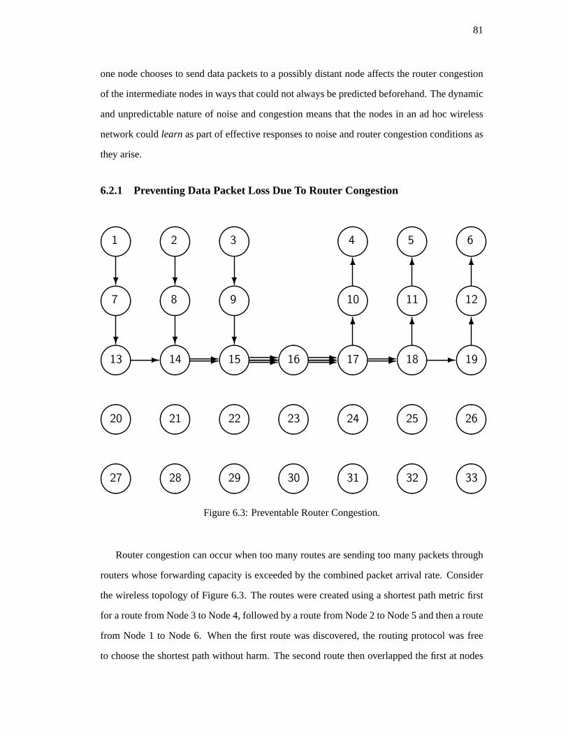
81

one node chooses to send data packets to a possibly distant node affectsthe router congestion

of the intermediate nodes in ways that could not always be predicted beforehand. The dynamic

and unpredictable nature of noise and congestion means that the nodes in an ad hoc wireless

network couldlearn as part of effective responses to noise and router congestion conditions as

they arise.

6.2.1 Preventing Data Packet Loss Due To Router Congestion

��

��

��

��

��

��

��

��

��

��

��

��

��

��

��

��

��

��

��

��

��

��

��

��

��

��

��

��

��

��

��

��

��

1 2 3 4 5 6

7 8 9 10 11 12

13 14 15 16 17 18 19

20 21 22 23 24 25 26

27 28 29 30 31 32 33

?

?- -- -- -

6

6?

?-- - - --

6

6?

?- -

6

6

Figure 6.3: Preventable Router Congestion.

Router congestion can occur when too many routes are sending too many packets through

routers whose forwarding capacity is exceeded by the combined packetarrival rate. Consider

the wireless topology of Figure 6.3. The routes were created using a shortest path metric first

for a route from Node 3 to Node 4, followed by a route from Node 2 to Node5 and then a route

from Node 1 to Node 6. When the first route was discovered, the routing protocol was free

to choose the shortest path without harm. The second route then overlapped the first at nodes

82

15, 16 and 17, requiring those nodes to forward packets for both routes. The third route then

overlapped the second at nodes 14 and 18, requiring them to forward packets for both routes

and adding to the workload of nodes 15, 16 and 17 by requiring them to nowforward packets

for three routes. Data packets start getting lost if the combined arrival rates at any node exceeds

its forwarding capacity. The loss of data packets could have been prevented because there are

other underutilized nodes available that could carry packets for all the routes without packet

loss.

The loss of data packets could be prevented during route discovery if thenodes sending

and forwarding data packets in the ad hoc network learned the combined data packet arrival

(and sending) rates. This rate is theλq portion of the formula for the component of the routing

metric described in Section 3.1 that represents the mean time a packet spends inthe router

before it is forwarded. Adding this component to the time it takes to forward apacket at the

MAC layer gives the time cost of moving data through the node. Later route discoveries using

Warp-5 would use the time cost in deciding the time-to-destination cost of each neighbor.

The time cost calculation Warp-5 uses in calculating time-to-destination comes from infor-

mation learned from experience with earlier routes in the ad hoc network.

6.2.2 Responding to Router Congestion To Prevent Data Packet Loss

Routers can still become congested, even when experience-based routing metrics are used in

the process of route discovery. Each route discovery attempts to find the best route from source

to destination without considering possible future routes. The potential forrouter congestion

arises when new routes are added to an otherwise congestion-free network. Consider the situa-

tion in the wireless ad hoc network depicted in Figure 6.4.

Here, the route from Node 3 to Node 4 was discovered first, followed by the router from

Node 1 to Node 6. The routes do not overlap and the traffic level does not exceed the forwarding

capacity of the routers. The problem of router congestion arises when Node 2 wants to send

data to Node 5. There is no route from Node 2 to Node 5 that does not use routers from a

previous route. If the combined traffic level on any node sending or forwarding data packets

for multiple routes exceeds its forwarding capacity, data packets will be dropped. The loss of

data packets is unnecessary and the router congestion can be repairedbecause there are other

83

��

��

��

��

��

��

��

��

��

��

��

��

��

��

��

��

��

��

��

��

��

��

��

��

��

��

��

��

��

��

��

��

��

1 2 3 4 5 6

7 8 9 10 11 12

13 14 15 16 17 18 19

20 21 22 23 24 25 26

27 28 29 30 31 32 33

?

?

?- - - - - -

6

6

6?

?

?

?- - - -

6

6

6

6?

?- -

6

6

Figure 6.4: Correctable Router Congestion.

underutilized nodes available that could carry packets for all the routes without packet loss.

A wireless ad hoc network using Warp-5 could resolve this problem using learned informa-

tion. The nodes would learn the order that routes were created, the data packet arrival rates for

specific routes, the link-level unicast times and the estimated time between the first appearance

of a detangling RREQ and the time the node stops receiving packets for a specific route. A node

whose data packet arrival rate exceeds its forwarding capacity will broadcast a special detan-

gling RREQ packet for one of the routes overloading it. Other nodes receiving this packet will

make routing decisions based only on the packet arrival rates for routes that were created after

the route specified in the detangling RREQ. It takes time for the detangling RREQto propagate

through the wireless network, for the route to change (if it changes at all)and for the nodes in

the network to recognize that the route has actually changed and not just experienced a brief

lull in offered load. The overloaded node that initially broadcast the detangling RREQ packet

will only detect a change in the route if the data arrival rate for that route reduces to zero. Other

84

nodes may experience overloading while the previous route is changing. In either event, further

detangling actions may be needed to alleviate router congestion, but each detangling effort re-

quires stable routes to ensure correct router load information. Nodes experiencing congestion

therefore have to estimate the time from the initial appearance of a detangling RREQ packet

until routes stabilize before attempting to detangle another route.

Nodes in a wireless ad hoc network using Warp-5 would also learn the data packet arrival

times for specific routes and recognize the time between the first appearance of a RREQ packet

for a specific route and the time the arrival rate for that route reduces to zero. An overloaded

node would use its learned time for the changed routes to stabilize before taking the next route

detangling step by broadcasting another RREQ packet. The subsequentroute re-discovery

would make use of link-level unicast times and data packet arrival rates,both learned from

recent experience of the nodes in the wireless network.

6.2.3 Preventing Data Packet Loss Due To Noise

Pre-existing noise sources in the wireless communication environment can cause the loss of

data packets. A weak noise source may not have a measurable effect ondata packet transmis-

sions. A very strong noise source may completely disrupt some links and prevent routers from

using these links. The problem is most interesting when the noise sources are strong enough to

interfere with data packet transmissions, but not strong enough to completely prevent the for-

mation of routes in the wireless ad hoc network. Consider the situation in the square topology

of Figure 6.5.

The noise source in the center of the topology is strong enough to disrupt data traffic trans-

mitted at high transmission rates and only partially disrupt data traffic transmitted at lower

transmission rates due to the greater resilience of modulations at lower transmission rates. The

routes were created using a shortest path metric, ignoring proximity to the disruptive noise

source. Many of the data packets transmitted along these routes are subsequently lost. The

loss of data packets is unnecessary and preventable because there are other underutilized nodes

available that could carry packets to their destination with smaller likelihood of packet loss.

A wireless ad hoc network using Warp-5 could minimize data packet loss usinginformation

learned from experience with link-level unicasts. In a noisy environment,the probability of a

85

Figure 6.5: Square Topology With Poorly Chosen Routes

link-level unicast transmission failing increases in relation to the signal-to-noise ratio. The

802.11 MAC wireless hardware automatically retries unicast transmission somefixed number

of times until the transmission is acknowledged. The probability of unicast failure and the

time taken to complete a unicast (whether resulting in success or failure) can be learned from

recent experience with link-level unicast transmissions. These factorsare part of the time-based

routing metric Warp-5 uses to select the next hop when forwarding data packets. In the square

topology, Nodes 9 and 15 have more than one neighbor available to select as the next hop.

Increasing packet loss from unicasts to Nodes 10 and 16 will increase the time cost of using

those nodes. Eventually, the time cost will be greater than the time cost of forwarding to Nodes

7 and 21, and the data packets will be directed away from the noise source.

86

6.2.4 Responding To Noise To Minimize Data Packet Loss

Noise sources that dynamically appear in the wireless environment used bya wireless ad hoc

network can also cause the loss of data packets. When the noise sourcesare strong enough to

interfere with data packet transmissions, but not strong enough to completely prevent the for-

mation of routes in the wireless ad hoc network, the loss of data packets neednot be inevitable.

Consider the situation in the square topology of Figure 6.6, which shows routes established

under noise-free conditions and three potential noise sources.

��

��

��

��

��

��

��

��

��

��

��

��

��

��

��

��

��

��

��

��

��

��

��

��

��

��

��

��

t

s

s

1 2 3 4 5 6

7 8

9 10 11 12 13 14

15 16 17 18 19 20

21 22

23 24 25 26 27 28

?- - - - -- - - - -

6

6

- - - - -- - - - -

?

- - - - -

- - - - -

Figure 6.6: Square Topology Before Noise Source Activation

Suppose that once activated, the noise source in the center of the topology is strong enough

to disrupt data traffic transmitted at high transmission rates, yet only partially disrupt data traffic

transmitted at lower transmission rates. Also, assume the routes were createdusing a shortest

path metric, before the noise sources were activated. When the noise sources become active,

many of the data packets transmitted along these routes would be lost. The loss of data packets

is unnecessary and correctable because there are other underutilizednodes available that could

87

carry packets to their destination with smaller likelihood of packet loss.

A wireless ad hoc network using Warp-5 could minimize data packet loss usinginformation

learned from experience with link-level unicasts when the noise levels change. The probability

of unicast failure and the time taken to complete a unicast (whether resulting in success or fail-

ure) can be learned from recent experience with link-level unicast transmissions in the changed

environment. These factors are part of the time-based routing metric Warp-5 uses to select the

next hop when forwarding data packets. In the square topology, Nodes 9 and 15 have more than

one neighbor available to select as the next hop. Increasing packet loss from unicasts to Nodes

10 and 16 will increase the time cost of using those nodes. Shortly thereafter, the time cost

will be greater than the time cost of forwarding to Nodes 7 and 21, and the data packets will be

directed away from the noise source. This example demonstrates how an adhoc network using

Warp-5 would adjust to changing environmental noise conditions.

6.3 Experimental Scenarios

This section describes the experimental scenarios used to investigate the noise and congestion

properties described in the previous section.


The first property to investigate is the prevention of data packet loss due torouter congestion

in wireless ad hoc networks. The exploration scenario for this problem requires that multiple

routes are established in a wireless topology simulation where the shortest path metric results in

router congestion and data packet loss. Warp-5 and AODV congestion-avoidance simulations

run on the static “castle” topology shown in Figure 6.1. The effective communication radius for

all nodes is 10 meters. The nodes are placed so that the nearest neighbors are 9 meters away.

The effect is that the transmission from a node will reach the neighbors above, below, left and

right of the transmitting node.

The nodes in the congestion-avoidance simulations are homogeneous with regard to packet

forwarding capacity and routing queue size. There are three routes to discover and use during

the simulation: Node 3 to Node 4, Node 2 to Node 5, and Node 1 to Node 6, all discovered

88

in that order for all simulations. Four router/radio configurations are runin the simulations:

AODV on single-radio nodes, AODV on dual-radio nodes, Warp-5 on single-radio nodes and

Warp-5 on dual-radio nodes. For each router/radio configuration, three simulations are run,

each with the routes taking a different proportion of the router forwarding capacity. The offered

load of each route in the “low” simulations is equivalent to 20 percent of the router forwarding

capacity, the offered load of each route in the “medium” simulations is equivalent to 40 percent

of router forwarding capacity and the offered load of each route in the “high” simulations is

equivalent to 66.67 percent of router forwarding capacity, making a dozen simulations in all.

The low, medium and high offered loads represent distinctly different congestion behaviors

relative to the router forwarding capacity rather than specific percentages. The route discovery

from Node 3 to Node 4 begins at the start of the simulation, the route discovery from Node 2 to

Node 5 begins 4.0 seconds into the simulation and the route discovery from Node 1 to Node 6

begins 8.0 seconds into the simulation. Each source node generates data packets at a constant

rate.

The offered load of the low simulations means that three routes could multiplex packets

through one or more nodes without packet loss because the combined packet arrival rate is still

less than the router forwarding capacity. Only two routes could multiplex the offered load of

the medium simulations without loss of packets. The offered load of each route in the high

simulations is large enough to mean that packet loss is minimized when no more than one node

is used in any single route. Each node has a non-zero time to forward and transmit a node to the

next hop on a route, so the first Warp-5 route discovery is free to select a node with the fewest

hops between source and destination. The second Warp-5 route discovery will have to consider

the effects of the first route when selecting a route that minimizes source-to-destination time.

The third Warp-5 route discovery will have to consider the effects of the first two routes when

selecting the route with the smallest source-to-destination time. Depending on theoffered load

offered by each route, the second and third routes may not always have the fewest hops in the

simulated topology.

Routers using AODV will always select the shortest visible route, which leads to intersect-

ing routes regardless of the load offered by the routes involved. Nodes15, 16 and 17 in the

castle topology are bottlenecks, suffering loss of data packets when the offered load exceeded

89

the router forwarding capacity.

Each simulation in this scenario runs for 120 (simulated) seconds.

6.3.2 Responding To Router Congestion To Minimize Data Packet Loss

The second property to investigate is the protocol’s response to router congestion and the mini-

mization of packet loss in wireless ad hoc networks. The exploration scenario for this problem

requires that multiple routes are established in a wireless topology simulation where the shortest

path metric results in router congestion and data packet loss. Warp-5 and AODV congestion-

response simulations run on the castle topology with the same effective communication radius

of 10 meters for all nodes. The nodes for the simulations are placed so thatthe nearest neigh-

bors are 9 meters away. The effect is that the transmission from a node reaches the neighbors

above, below, left and right of the transmitting node.

The nodes in the congestion-response simulations are homogeneous with regard to packet

forwarding capacity and routing queue size. There are three routes to establish and use during

the simulation: Node 3 to Node 4, Node 2 to Node 5, and Node 1 to Node 6. Simulations

run with four router/radio configurations: AODV on single-radio nodes,AODV on dual-radio

nodes, Warp-5 on single-radio nodes and Warp-5 on dual-radio nodes. Six different simulations

run for each router/radio configuration with the three different routes discovered in different

orders for a total of 24 simulations in all. The first route discovery begins at the start of the

simulation, the second discovery begins 4.0 seconds into the simulation and the third route

discovery begins 8.0 seconds into the simulation. Each source node generates data packets

at a constant rate equal to two-thirds of the router forwarding capacity.Thus, any two routes

using the same node send traffic at a combined rate that exceeds the forwarding capacity of

that node’s router by 33.33 percent, resulting in a 25 percent loss of data packets. Three routes

sharing the name node send traffic at a combined rate twice that of the forwarding capacity of

the router, resulting in a 50 percent loss of data packets.

Setting the offered load for each route at two-thirds of router forwarding capacity means

that expected time to move a packet from source to destination for each routein the simulated

topology is minimized when all three routes do not overlap (i.e. no node is usedin more than

one route). Each node has a non-zero time to forward and transmit a nodeto the next hop

90

on a route, so the first Warp-5 route discovery is free to select a node with the fewest hops

between source and destination. The second Warp-5 route discovery will have to consider

the effects of the first route when selecting a route that minimizes source-to-destination time.

The third Warp-5 route discovery will have to consider the effects of the first two routes when

selecting the route with the smallest source-to-destination time. Depending on theorder in

which the routes were created, the three routes may intersect and result incongested routers in

the simulation topology.

Routers using AODV will always select the shortest visible route, which leads to intersect-

ing routes and congested routers in the simulation topology, regardless of the order in which

the routes were created. The nodes 15, 16 and 17 will be bottleneck nodes when the shortest

route is selected for more than one of the desired routes.

Each simulation for this scenario runs for 300 (simulated) seconds.


The third property to investigate is the prevention of data packet loss due to noise in the wireless

network environment. The exploration scenario for this problem requiresthat multiple routes

are established in a wireless topology simulation where the shortest path metric results in data

packet loss due to proximity to a noise source. Warp-5 and AODV noise-avoidance simulations

run on the square topology with an effective communication radius for all nodes of 10 meters.

The nodes are placed so that the nearest neighbors are 9 meters away.The effect is that the

transmission from a node reaches the neighbors above, below, left andright of the transmitting

node.

The nodes in the noise-avoidance simulations are homogeneous with regardto packet for-

warding capacity and routing queue size. There are six routes to establishand use during the

simulations. The route discoveries for Node 1 to Node 6, Node 9 to Node 14 and Node 21

to Node 22 begin at the start for the simulation and the route discoveries for Node 7 to Node

8, Node 15 to Node 20 and Node 23 to Node 28 begin 1.0 seconds into the simulation. Each

node generates data packets at a constant rate. A noise source is placed at the geometric center

of the topology, between Nodes 11, 12, 17 and 18. The noise source is calibrated to cause

a 50 percent loss of 500 byte packets transmitted at 6 Mbits/sec on links between Nodes 11,

91

12, 17 and 18. Two other less powerful noise sources are placed in twocorners of the square

topology. These sources are calibrated to cause a 10 percent loss of 500 byte data packets

transmitted at 54 Mbits/sec on the links between the nearest nodes. Simulations run with four

router/radio configurations: AODV on single-radio nodes, AODV on dual-radio nodes, Warp-5

on single-radio nodes and Warp-5 on dual-radio nodes. For each router/radio configuration, one

simulation runs with the default transmission rate of 54 Mbits/sec, and another simulation runs

with the default transmission rate of 6 Mbits/sec. The 54 Mbits/sec rate is the fastest 802.11g

transmission rate, and it is the rate that is the least resilient to noise. The 6 Mbits/sec rate is the

slowest 802.11g transmission rate, but it is the rate that is the most resilient to noise.

The performance issue explored in these simulations is how many application data packets

actually arrive at their intended destination. Warp-5 is free to select alternate routes for any

source-to-destination pair as needed using routing information from the RREQ/RREP packets

not lost due to noise. AODV will always choose the shortest route constructible from the

RREQ/RREP control packets not lost due to noise.



The fourth property to investigate is the response to new noise sources and the minimization

of data packet loss in the wireless ad hoc network. The exploration scenario for this problem

requires multiple route discoveries in an initially noise-free wireless topology simulation envi-

ronment. Once the routes were established and data traffic was moving through the network,

multiple noise sources are then activated. Warp-5 and AODV noise-injectionsimulations run

on the square topology with an effective communication radius for all nodesof 10 meters.

The nodes are placed so that the nearest neighbors are 9 meters away.The effect is that the

transmission from a node reaches the neighbors above, below, left andright of the transmitting

node.

The nodes are homogeneous with regard to packet forwarding capacityand routing queue

size. There are six routes to establish and use during the simulations. The route discoveries

for Node 1 to Node 6, Node 9 to Node 14 and Node 21 to Node 22 begin at thestart for the

simulation and the route discoveries for Node 7 to Node 8, Node 15 to Node 20and Node 23 to

92

Node 28 begin 1.0 seconds into the simulation. Each node generates data packets at a constant

rate. A noise source is placed at the geometric center of the topology, between Nodes 11, 12, 17

and 18. The noise source is be calibrated to cause a 50 percent loss of 500 byte packets trans-

mitted at 6 Mbits/sec on links between Nodes 11, 12, 17 and 18. Two other lesspowerful noise

sources are placed in two corners of the square topology. These sources are calibrated to cause

a 10 percent loss of 500 byte data packets transmitted at 54 Mbits/sec on the links between the

nearest nodes. The three noise sources activate 4.0 seconds into the simulation. Simulations

run with four router/radio configurations: AODV on single-radio nodes,AODV on dual-radio

nodes, Warp-5 on single-radio nodes and Warp-5 on dual-radio nodes. For each router/radio

configuration, one simulation runs with the default transmission rate of 54 Mbits/sec, and an-

other simulation runs with the default transmission rate of 6 Mbits/sec. The 54 Mbits/sec rate

is the fastest 802.11g transmission rate, but the least resilient to noise while the 6 Mbits/sec rate

is the slowest 802.11g transmission rate, and the most resilient to noise.

The performance issue explored in these simulations is how many application data packets

actually arrive at their intended destination. Warp-5 is free to select alternate routes for any

source-to-destination pair as needed using routing information learned during the initial route

discoveries. AODV will always choose the shortest routes between source and destination.


6.4 Simulation Results and Discussion

This section contains descriptions of the simulation results related to managing noise and con-

gestion in wireless ad hoc networks. There are several problems explored in the simulations.

The first problem concerns the prevention of data packet loss due to improper route construc-

tion. The second concerns the response to router congestion when it occurs. The third concerns

the construction of routes in a noisy environment to minimize data packet loss, and the fourth

concerns the response to noise that arises in the wireless environment after routes have been

established.

93


The objective of the congestion-avoidance simulations was to show that Warp-5 could effec-

tively prevent router congestion and packet loss in wireless ad hoc networks. Figures 6.7, 6.8

and 6.9 plot application data packet arrival rate over time throughout the 120-second simula-

tion runs. The packet arrival rate was sampled every 1/10 of a (simulated) second. Both Warp-5

and AODV used expanding ring searches with identical interval and time-to-live parameters to

find initial routes. Each router forwarded packets as an exponential server with a mean service

capacity of 50 packets per second (i.e. an average of 0.02 seconds between packets). For the

low offered load simulations, each source node generated 500-byte datapackets at a constant

rate of 10 per second. For the medium offered load simulations, each source node generated

500-byte data packets at a constant rate of 20 per second. For the highoffered load simulations,

each source node generated 500-byte data packets at a constant rateof 33.33 per second.

0

20

40

60

80

100

120

140

0 20 40 60 80 100 120

Tot

al d

ata

pack

et a

rriv

al r

ate

(pac

kets

per

sec

ond)

Time (seconds)

AODV one radioAODV two radios

0

20

40

60

80

100

120

140

0 20 40 60 80 100 120

Tot

al d

ata

pack

et a

rriv

al r

ate

(pac

kets

per

sec

ond)

Time (seconds)

Warp-5 one radioWarp-5 two radios

(a) AODV on single-radio and dual-radio (b) Warp-5 on single-radio and dual-radionodes nodes

��

��

��

��

��

��

��

��

��

��

��

��

��

��

��

��

��

��

��

��

��

��

��

��

��

��

��

��

��

��

��

��

��

?- -

?- -

6

- -

6?

-

?- -

6

6

-

?

?- -

6

6

1 2 3 4 5 6

7 8 9 10 11 12

13 14 15 16 17 18 19

20 21 22 23 24 25 26

27 28 29 30 31 32 33

��

��

��

��

��

��

��

��

��

��

��

��

��

��

��

��

��

��

��

��

��

��

��

��

��

��

��

��

��

��

��

��

��

?-

?- - - - -

6

6

-

?

?- - -

6

6?

?- -

6

6

1 2 3 4 5 6

7 8 9 10 11 12

13 14 15 16 17 18 19

20 21 22 23 24 25 26

27 28 29 30 31 32 33

(c) Typical AODV routes (d) Typical Warp-5 routes

Figure 6.7: AODV and Warp-5 Data Packet Arrival Rates For Low Offered Load Simulations

94

The plots of data packet arrival rates for three routes as a function oftime are shown for

AODV in Figure 6.7(a) and for Warp-5 in Figure 6.7(b) for the low offered load simulations

using single-radio and dual-radio nodes. With the total offered load for the three routes being

less than the router forwarding capacity, all three routes can share the shortest path from source

to destination in Warp-5. For AODV, the shortest path was sufficient for all three routes without

router congestion. All four router/radio configurations maintained a total data packet arrival rate

of 30 packets per second in the 120-second simulation run. The route discovery for the third

route under AODV on single-radio nodes conflicted with the surge of packets initially buffered

from the second route, delaying the completion of the third route discovery briefly as visible in

the figure. If the offered load is low enough, as they were in this simulation, Warp-5 selected the

shortest route. Castle topologies for AODV in Figure 6.7(c) and for Warp-5 in Figure 6.7(d)

show typical routes from the low offered load simulations. The routes selected by AODV and

Warp-5 in the low offered load simulations deliver data packets at the same rate and are not

significantly different.


AODV in Figure 6.8(a) and for Warp-5 in Figure 6.8(b) for the medium offered load simula-

tions using single-radio and dual-radio nodes. The total offered load for all three routes was 60

data packets per second. AODV chose the shortest path for all three routes, with some routers

receiving data packets at a rate that exceeded their forwarding capacity of only 50 packets per

second. With the medium offered load, AODV fell short of the offered load by 10 packets

per second. For the Warp-5 simulations, the router forwarding capacity was high enough for

Nodes 15, 16 and 17 to support the first two routes with minimal time cost. The third route

did not intersect the previous two routes at all, resulting in a sustained data packet arrival rate

that matched the offered load of 60 packets per second. Castle topologies for AODV in Fig-

ure 6.8(c) and for Warp-5 in Figure 6.8(d) show typical routes from themedium offered load

simulations.


AODV in Figure 6.9(a) and for Warp-5 in Figure 6.9(b) for the high offered load simulations

using single-radio and dual-radio nodes. With each of the three routes requiring more than

half of the router forwarding capacity, none of the three routes could share a router without

95

0

20

40

60

80

100

120

140

0 20 40 60 80 100 120

Tot

al d

ata

pack

et a

rriv

al r

ate

(pac

kets

per

sec

ond)

Time (seconds)


0

20

40

60

80

100

120

140

0 20 40 60 80 100 120

Tot

al d

ata

pack

et a

rriv

al r

ate

(pac

kets

per

sec

ond)

Time (seconds)



��

��

��

��

��

��

��

��

��

��

��

��

��

��

��

��

��

��

��

��

��

��

��

��

��

��

��

��

��

��

��

��

��

- -

?

?- -

6

-

6

--

?

?- -

6

6

-

?

?- -

6

6

1 2 3 4 5 6

7 8 9 10 11 12

13 14 15 16 17 18 19

20 21 22 23 24 25 26

27 28 29 30 31 32 33

��

��

��

��

��

��

��

��

��

��

��

��

��

��

��

��

��

��

��

��

��

��

��

��

��

��

��

��

��

��

��

��

��

?

?

?- - - - - -

6

6

6?

?- - - -

6

6?

?- -

6

6

1 2 3 4 5 6

7 8 9 10 11 12

13 14 15 16 17 18 19

20 21 22 23 24 25 26

27 28 29 30 31 32 33

(c) Typical AODV routes (d) Typical Warp-5 routes

Figure 6.8: AODV and Warp-5 Data Packet Arrival Rates For Medium Offered Load Simula-tions

losing data packets. AODV on dual-radio nodes chose the shortest path for all three routes,

with some routers receiving data packets at a rate that exceeded their forwarding capacity of

only 50 packets per second. With the high offered load, AODV on dual-radio nodes lost data

packets at a rate of 50 packets per second.

AODV on single-radio nodes actually outperformed AODV on dual-radio nodes. The of-

fered load of the first two routes repeatedly thwarted route discovery attempts for the third

route, reducing the total data packet arrival rate for almost 50 seconds into the simulation.

The eventual completion of the third route discovery resulted in a route that did not share any

nodes with those used by the first two routes. This example clearly illustrates how AODV im-

plicitly handles congestion. AODV interpreted the highly congested routers as “down” during

the third route discovery and appropriately found a route that avoided thecongested routers.

96

0

20

40

60

80

100

120

140

0 20 40 60 80 100 120

Tot

al d

ata

pack

et a

rriv

al r

ate

(pac

kets

per

sec

ond)

Time (seconds)


0

20

40

60

80

100

120

140

0 20 40 60 80 100 120

Tot

al d

ata

pack

et a

rriv

al r

ate

(pac

kets

per

sec

ond)

Time (seconds)



��

��

��

��

��

��

��

��

��

��

��

��

��

��

��

��

��

��

��

��

��

��

��

��

��

��

��

��

��

��

��

��

��

?

?

?- - - - - -

6

6

6?

-

?- -

6

6

-

?

?- -

6

6

1 2 3 4 5 6

7 8 9 10 11 12

13 14 15 16 17 18 19

20 21 22 23 24 25 26

27 28 29 30 31 32 33

��

��

��

��

��

��

��

��

��

��

��

��

��

��

��

��

��

��

��

��

��

��

��

��

��

��

��

��

��

��

��

��

��

?

?

?

?- - - - - -

6

6

6

6?

?

?- - - -

6

6

6?

?- -

6

6

1 2 3 4 5 6

7 8 9 10 11 12

13 14 15 16 17 18 19

20 21 22 23 24 25 26

27 28 29 30 31 32 33

(c) AODV routes (single radio) (d) Warp-5 routes (single- and dual-radio)

Figure 6.9: AODV and Warp-5 Data Packet Arrival Rates For High Offered Load Simulations

However, because the handling of router congestion is implicit, the use of a second radio ac-

tually makes route discovery worse–AODV wouldn’t notice that some routers are congested

and would continue to assign new routes to congested routers. By explicitly measuring and

considering congestion delays, Warp-5 much more adeptly handled the router congestion.

The total data packet arrival rate for these three routes was 83.33 datapackets per second,

falling short of the offered load by 16.66 data packets per second, butsingle-radio AODV still

outperformed AODV on dual-radio nodes. Warp-5 managed the high offered loads by finding

separate routes that did not share any nodes. The dual-radio configuration of Warp-5 found the

three routes slightly faster than Warp-5 on single-radio nodes, but both Warp-5 configurations

found routes whose total data packet arrival rate matched the total offered load of 100 data

packets per second without data loss. Castle topologies for AODV in Figure6.9(c) and for

Warp-5 in Figure 6.9(d) show typical routes from the high offered load simulations.

97

0

2000

4000

6000

8000

10000

12000

Low Medium High

Tot

al P

acke

ts D

eliv

ered

AODV single−radioAODV dual−radioWarp−5 single−radioWarp−5 dual−radio

Figure 6.10: Preventing Router Congestion.

The results of the individual congestion-avoidance simulations for both protocols using

single-radio and dual-radio nodes are shown in Figure 6.10. The vertical axis is the number of

application data packets delivered during the simulation. AODV and Warp-5 on single-radio

nodes and dual-radio nodes delivered about the same number of data packets in the low load

simulations. With the offered load of each route requiring only 10 packets per second, the use

of single- or dual-radio nodes was not significant for either protocol. In the medium offered

load simulations, AODV added a third route that intersected the previous routes, resulting in

router congestion and data packet loss. Warp-5 outperformed AODV byadding a third route

that did not compete with the previous routes for router resources. AODVon single-radio

nodes outperformed AODV on dual-radio nodes in the high load simulations, but both were

outperformed by Warp-5 on single-radio nodes or dual-radio nodes. By learning the router

forwarding time cost of previously established routes, Warp-5 was able touse this information

to select sensible routes that could deliver data packets at the same rate they were offered in all

three situations.

The results of the congestion-avoidance experiments shows the feasibility and usefulness of

learning router forwarding time cost from recent experience with current network conditions in

98

avoiding router congestion in wireless ad hoc networks and improving distributed application

throughput consistent with the thesis of this dissertation.

6.4.2 Responding To Router Congestion To Minimize Data Packet Loss

The objective of the congestion-response simulations was to show that Warp-5 could effectively

respond to router congestion bottlenecks as they arise in wireless ad hoc networks. Figures 6.11

and 6.12 plot application data packet arrival rate over time throughout the 300-second simula-

tion runs. The packet arrival rate was sampled every 1/10 of a (simulated) second. Both Warp-5

and AODV used expanding ring searches with identical interval and time-to-live parameters to

find initial routes. Each source node generated data packets at a constant rate of 33.33 packets

per second (0.03 seconds between packets). Each router forwarded packets as an exponential

server with a mean service capacity of 50 packets per second (0.02 seconds between packets).

0

20

40

60

80

100

120

140

0 50 100 150 200 250 300

Tot

al d

ata

pack

et a

rriv

al r

ate

(pac

kets

per

sec

ond)

Time (seconds)

AODV one radio 123AODV one radio 132AODV one radio 312AODV one radio 213AODV one radio 231

0

20

40

60

80

100

120

140

0 50 100 150 200 250 300

Tot

al d

ata

pack

et a

rriv

al r

ate

(pac

kets

per

sec

ond)

Time (seconds)

Warp-5 one radio 123Warp-5 one radio 132Warp-5 one radio 312Warp-5 one radio 213Warp-5 one radio 231

(a) AODV on single-radio nodes (b) Warp-5 on single-radio nodes

��

��

��

��

��

��

��

��

��

��

��

��

��

��

��

��

��

��

��

��

��

��

��

��

��

��

��

��

��

��

��

��

��

-

?-

?- -

6

-

6

--

?

?- -

6

6

-

?

?- -

6

6

1 2 3 4 5 6

7 8 9 10 11 12

13 14 15 16 17 18 19

20 21 22 23 24 25 26

27 28 29 30 31 32 33

��

��

��

��

��

��

��

��

��

��

��

��

��

��

��

��

��

��

��

��

��

��

��

��

��

��

��

��

��

��

��

��

��

?

?

?

?- - - - - -

6

6

6

6?

?

?- - - -

6

6

6?

?- -

6

6

1 2 3 4 5 6

7 8 9 10 11 12

13 14 15 16 17 18 19

20 21 22 23 24 25 26

27 28 29 30 31 32 33

(c) Typical AODV routes (d) Detangled Warp-5 routes

Figure 6.11: AODV and Warp-5 Data Packet Arrival Rates For Router Congestion Problems(single-radio nodes).

99

The total data packet arrival rates as a function of time are plotted for fiverouter congestion

tests for AODV on single-radio nodes in Figure 6.11(a). In the AODV simulations, one test

found a route within a couple of seconds and started sending buffered packets through the

network at the maximum forwarding rate of 50 packets per second. The application packet

arrival rate for this test and the other five tests was quickly reduced by the loss of application

data packets due to route discovery packets contending for the same router input queues. The

tests took between 40 and 60 seconds to find routes for all three source-destination pairs. The

delay in some of the tests finding the right route was the result of repeated thwarted attempts

due to the inability to get RREQ and RREP packets past the congested routers. The result is a

data packet arrival rate plot that is far below the expected rate of 50 packets per second for much

of the simulation. The castle topology of Figure 6.11(c) shows the routes forthe single-radio

AODV simulations.

Figure 6.11(b) shows the simulation results for Warp-5 on single-radio nodes. With con-

gested routers, detangling RREQ and RREP packets either took longer to move through the

network or got dropped by some nodes, which slowed the detangling process. The route detan-

gling caused the high variability in data packet arrival rates in the early part of the simulation.

One of the fives tests, actually had the routes detangled correctly a few seconds into the simula-

tion, but because it lacked sufficient experience to estimate how long it tookpacket arrival rates

to stabilize after a route change, prematurely continued to change routes and continued detan-

gling until it returned to the correct route detangling about 150 seconds into the simulation.

Once routes were detangled, the average data packet arrival rate became consistent with the

data packet generation rate of 100 data packets per second. The remaining variability after the

route detangling was due to the exponential service process of the routers. The castle topology

of Figure 6.11(d) shows the detangled routes for the single-radio Warp-5 simulations.

The total data packet arrival rates as a function of time are plotted in Figure6.12(a) for five

router congestion tests for AODV using dual radios. In the AODV simulations, route discovery

is much faster with all three routes in all five tests completed in the first 10 seconds because

the RREQ and RREP packets could move through the network without contentionfrom data

packets for router input queues. The variability in application data packetarrival rates once

routes were established is due to the exponential service function in the router forwarding

100

0

20

40

60

80

100

120

140

0 50 100 150 200 250 300

Tot

al d

ata

pack

et a

rriv

al r

ate

(pac

kets

per

sec

ond)

Time (seconds)

AODV two radios 123AODV two radios 132AODV two radios 312AODV two radios 213AODV two radios 231

0

20

40

60

80

100

120

140

0 50 100 150 200 250 300

Tot

al d

ata

pack

et a

rriv

al r

ate

(pac

kets

per

sec

ond)

Time (seconds)

Warp-5 two radios 123Warp-5 two radios 213Warp-5 two radios 312Warp-5 two radios 213Warp-5 two radios 231

(a) AODV on dual-radio nodes (b) Warp-5 on dual-radio nodes

��

��

��

��

��

��

��

��

��

��

��

��

��

��

��

��

��

��

��

��

��

��

��

��

��

��

��

��

��

��

��

��

��

-

?-

?- -

6

-

6

-

?-

?- -

6

6

-

?

?- -

6

6

1 2 3 4 5 6

7 8 9 10 11 12

13 14 15 16 17 18 19

20 21 22 23 24 25 26

27 28 29 30 31 32 33

��

��

��

��

��

��

��

��

��

��

��

��

��

��

��

��

��

��

��

��

��

��

��

��

��

��

��

��

��

��

��

��

��

?

?

?

?- - - - - -

6

6

6

6?

?

?- - - -

6

6

6?

?- -

6

6

1 2 3 4 5 6

7 8 9 10 11 12

13 14 15 16 17 18 19

20 21 22 23 24 25 26

27 28 29 30 31 32 33

(c) Typical AODV routes (d) Detangled Warp-5 routes

Figure 6.12: AODV and Warp-5 Data Packet Arrival Rates For Router Congestion Problems(dual-radio nodes).

times. AODV on dual-radio nodes found the same routes as AODV on single-radio nodes,

but the dual-radio configuration performed better because the RREQ andRREP packets could

move through the network faster on dual-radio nodes. The castle topologyof Figure 6.12(c)

shows the routes for the dual-radio AODV simulations.

Figure 6.12(b) shows the results for Warp-5 using dual radios. With the ability to move

RREQ and RREP packets through the network unaffected by congested data input queues, all

five tests found stable routes faster than Warp-5 on single-radio nodes.Stable routes with a total

packet delivery rate of 100 data packets per second took between 11 and about 70 seconds to

find, including time for initial route discovery. The higher variability in data packet arrival rates

between 10 and about 70 seconds is due to changing routes during detangling as the network

tried different routes. Any variation after that point in time is due to exponential service rates

in the individual routers. The castle topology of Figure 6.12(d) shows thedetangled routes for

the dual-radio Warp-5 simulations.

101

0

0.5

1

1.5

2

2.5

3x 10

4

123 132 312 213 231

Tot

al P

acke

ts D

eliv

ered


Figure 6.13: Adjusting to Router Congestion.

The results of the individual congestion-response simulations for both protocols using sin-

gle and dual radios are shown in Figure 6.13. The vertical axis is the number of application

data packets delivered during each simulation. The horizontal axis identifies the order of route

discovery in each test. AODV with dual radios slightly outperforms AODV on single-radio

nodes because the route discoveries were not affected by previous traffic in the dual-radio con-

figuration. AODV with either radio configuration found the shortest route between source

and destination regardless of existing data traffic. Warp-5 on single-radio nodes outperformed

AODV in all five test cases, demonstrating that the detangling algorithm workseven when the

propagation of RREQ and RREP packets is hampered by congested routers. Warp-5 on dual-

radio nodes consistently outperformed Warp-5 on single-radio nodes and AODV with single-

or dual-radios.

The superior performance of Warp-5 is attributable to its ability to learn and respond.

Routers learn the order in which routes were created and share different (pretended) route

creation orders during detangling to coordinate detangling efforts within thead hoc network.

Individual routers learn their own data packet arrival rates from recently received unicasts, and

when congested, can alter routes as needed. Routers also learn an estimate of how long it takes

102

for a route alteration to stabilize with the ad hoc network as part of the coordinated route detan-

gling effort. Warp-5 learned from recent learned experience with route creation and congestion

levels to deal with router congestion in a heavily-used network environment.

The results of the congestion-response experiments shows the feasibility and usefulness of

learning router forwarding time cost from recent experience with current network conditions to

adjust existing routes in wireless ad hoc networks to correct for router congestion and improve

distributed application throughput consistent with the thesis of this dissertation.


The purpose of the noise-avoidance simulations was to show that Warp-5 could minimize data

packet loss by building routes for an ad hoc network operating in a noisy environment. Figures

6.14 and 6.15 plot application data packet arrival rate throughout the 20-second simulation

runs. The packet arrival rate was sampled every 1/10 of a (simulated) second. Both Warp-5 and

AODV used expanding ring searches with identical interval and time-to-liveparameters to find

initial routes. Each source node generated data packets at a constant rate of 33.33 packets per

second (i.e. 0.03 seconds between packets). Each router forwardedpackets as an exponential

server with a mean service capacity of 10,000 packets per second (i.e. 0.0001 seconds between

packets), which allowed the routers to potentially share all the routes in the square topology

without becoming congested. The simulations remain valid because the combinedoffered load

of all routes did not approach the maximum packet flow rate for any unicast transmission rate,

much less the high forwarding rate of the routers.

Figure 6.14(a) shows the simulation results for AODV where the default transmission rate

was 54 Mbits/sec. AODV on single- or dual-radio nodes performed poorlybecause the 54

Mbits/sec transmission rate was very susceptible to noise. The single-radio configuration was

able to establish and use only two of the six routes. The powerful noise source at the center of

the topology prevented the completion of most of the route discoveries due to loss of RREQ and

RREP packets. The dual-radio configuration was able to establish all six routes, but the routes

were built using the shortest path metric, which resulted in routes passing near the powerful

central noise source and significant loss of data packets due to that proximity. The data packet

delivery rate for AODV in either configuration was only 7 to 10 packets persecond out of a

103

0

50

100

150

200

250

300

0 2 4 6 8 10 12 14 16 18 20

Tot

al d

ata

pack

et a

rriv

al r

ate

(pac

kets

per

sec

ond)

Time (seconds)

AODV one radio 54 Mbits/secAODV two radios 54 Mbits/sec

0

50

100

150

200

250

300

0 2 4 6 8 10 12 14 16 18 20

Tot

al d

ata

pack

et a

rriv

al r

ate

(pac

kets

per

sec

ond)

Time (seconds)

Warp-5 two radios 54 Mbits/secWarp-5 one radio 54 Mbits/sec


��

��

��

��

��

��

��

��

��

��

��

��

��

��

��

��

��

��

��

��

��

��

��

��

��

��

��

��

tgk� ��

��

sgk� ��

sgk� ��

- - - - -

6

- - - - -

?

6

- - - - -

?

- - - - -

1 2 3 4 5 6

7 8

9 10 11 12 13 14

15 16 17 18 19 20

21 22

23 24 25 26 27 28

��

��

��

��

��

��

��

��

��

��

��

��

��

��

��

��

��

��

��

��

��

��

��

��

��

��

��

��

tgk� ��

��

sgk� ��

sgk� ��

- - - - -

6

- - - - -

?

?

?

?- - - - -

6

6

66

6

6

- - - - -

?

?

?

?- - - - -

6

- - - - -

1 2 3 4 5 6

7 8

9 10 11 12 13 14

15 16 17 18 19 20

21 22

23 24 25 26 27 28

(c) Typical AODV routes (d) Improved Warp-5 routes

Figure 6.14: AODV and Warp-5 Data Packet Arrival Rates For 54 Mbits/sec in a noisy envi-ronment.

total offered load of 200 packets per second. The square topology ofFigure 6.14(c) shows the

routes for the single-radio and dual-radio AODV simulations for the 54 Mbits/sec transmission

rate.

The simulation results for Warp-5 using a default transmission rate of 54 Mbits/sec appear

in Figure 6.14(b). Warp-5 was able to establish all six routes despite the noise, although the

dual-radio configuration did so slightly faster than the single-radio configuration. In both cases,

Warp-5 raised the data packet arrival rate to match the offered load of 200 packets per second.

It did so by finding better unicast transmission rates and selecting better next hops from ex-

perience gained during forwarding. The improved data packet arrival rate continued to vary

throughout the remainder of the simulation. The square topology of Figure 6.14(d) shows the

improved routes for the single-radio and dual-radio Warp-5 simulations forthe 54 Mbits/sec

transmission rate.

104

0

50

100

150

200

250

300

0 2 4 6 8 10 12 14 16 18 20

Tot

al d

ata

pack

et a

rriv

al r

ate

(pac

kets

per

sec

ond)

Time (seconds)


0

50

100

150

200

250

300

0 2 4 6 8 10 12 14 16 18 20

Tot

al d

ata

pack

et a

rriv

al r

ate

(pac

kets

per

sec

ond)

Time (seconds)



��

��

��

��

��

��

��

��

��

��

��

��

��

��

��

��

��

��

��

��

��

��

��

��

��

��

��

��

tgk� ��

��

sgk� ��

sgk� ��

- - - - -

6

- - - - -

?

?- - - - -

6

- - - - -

- - - - -

- - - - -

1 2 3 4 5 6

7 8

9 10 11 12 13 14

15 16 17 18 19 20

21 22

23 24 25 26 27 28

��

��

��

��

��

��

��

��

��

��

��

��

��

��

��

��

��

��

��

��

��

��

��

��

��

��

��

��

tgk� ��

��

sgk� ��

sgk� ��

- - - - -

6

- - - - -

?

6

6

- - - - -

?

?

?

?- - - - -

6

6

?- - - - -- - - - -

1 2 3 4 5 6

7 8

9 10 11 12 13 14

15 16 17 18 19 20

21 22

23 24 25 26 27 28


Figure 6.15: AODV and Warp-5 Data Packet Arrival Rates For 6 Mbits/sec in a noisy environ-ment.


was 6 Mbits/sec. AODV on single-radio nodes was able to establish all six routes, but two of

the routes were in close proximity to the powerful noise source at the centerof the topology,

which resulted in the loss of half the packets on those two routes. The total data packet arrival

rate for AODV on single-radio nodes was about 150 packets per second. AODV on dual-radio

nodes also established all six routes, but three of the routes were near the central noise source

and half the data packets on three routes were lost, which reduced the datapacket arrival rate to

less than the rate experienced with the AODV single-radio simulation. The reduced data packet

arrival rate experienced in the dual-radio AODV simulation was due to the poor arbitrary choice

of three routes with nodes in close proximity to the central noise source and isnot related to

the use of single- or dual-radio nodes. The square topology of Figure 6.15(c) shows the routes

for the single-radio and dual-radio AODV simulations for the 6 Mbits/sec transmission rate.

105

The Warp-5 plots of Figure 6.15(b) shows the higher data packet arrival rate for Warp-5

with single- or dual-radio nodes. Warp-5 on single-radio nodes was ableto establish all six

routes, and raised the data packet arrival rate to 200 data packets persecond by finding better

unicast transmission rates and selecting better next hops from experience gained during packet

forwarding. The improved data packet arrival rate continued to vary throughout the remainder

of the simulation. Warp-5 on dual-radio nodes was able to establish routes somewhat faster

using the second radio and succeeded in establishing all six routes and raising the data packet

arrival rate to about 200 packets per second to match the total offered load. The data packet

arrival rate also continued to vary throughout the remainder of the simulation. Figure 6.15(c)

shows the routes for the single-radio and dual-radio Warp-5 simulations for the 6 Mbits/sec

transmission rate in the square topology.

Both the AODV plots show a stable data packet arrival rate, while the Warp-5 plots are more

variable. The intermittent drops and rises in the Warp-5 data packet arrival rates are caused by

random and transient asymmetries between the data packet arrival rate and the data packet for-

warding rate at the MAC layer for nodes in the wireless network. Such an asymmetry may arise

when there are many packets arriving at an intermediate wireless node with ahigh forwarding

rate. In forwarding a packet to the next hop, the MAC 802.11 random exponential backoff used

to control access to the communications medium sometimes chooses a large backoff counter,

which means a longer wait to transmit the packet to the next hop. The simultaneous arrival of

many packets to the same node during the backoff would delay the decrementing of the back-

off counter, further preventing the forwarding transmission while incomingpackets continue

to arrive and get added to the outgoing packet queue in the MAC card. The MAC outgoing

packet queue would quickly fill to capacity and further outgoing packets would get dropped

at the MAC layer. The delay in transmitting the packet at the front of the queue appears as a

drop in the data packet arrival rate in the Warp-5 plots. Eventually, the MAC layer does trans-

mit the packet and succeeds in transmitting the other packets in the queue quickly because of

small random backoff counters used for the later packets. This effectappears in the plots as

the immediately following increases in data packet arrival rates. Unfortunately, because data

packets were dropped from the outgoing MAC queue, the subsequent increases in data packet

transmissions from the node never compensate for the lost packets, whichreduces the total

106

number of data packets delivered to their destination node. These MAC-level asymmetries

occur randomly and are transient. They do not become less likely over time.

The AODV and Warp-5 routers used the same MAC layer implementation, but theAODV

simulations did not suffer from this random asymmetry because none of the AODV simulations

ever sent a high enough offered load through any intermediate nodes to experience the effect.

The AODV simulations never sent the traffic for more than two routes throughany intermediate

node. The Warp-5 simulations sent as many as four routes of traffic through some intermediate

nodes to avoid noise. The internal forwarding speed of the routers wasmore than fast enough

to handle the offered load from all six routes, but the offered load fromas few as three routes

was sufficient to cause the asymmetry to occur in the simulations.

0

500

1000

1500

2000

2500

3000

3500

54 Mbits/sec 6 Mbits/sec

Tot

al P

acke

ts D

eliv

ered


Figure 6.16: Preventing Data Packet Loss In Noisy Environment

The results of the individual noise-avoidance simulations for both protocols using 6 Mbits/sec

and 54 Mbits/sec as the default transmission rate are shown in Figure 6.16. The vertical axis

is the number of application data packets delivered over the course of the simulation. The

horizontal axis identifies the initial (or for AODV, fixed) link-level transmission rate. AODV

on single-radio nodes outperforms AODV on dual-radio nodes for the slowest and most noise-

resilient transmission rate, because of the effects of noise on route discovery. AODV with the

107

fastest transmission rate performed the worst, on single-radio nodes or dual-radio nodes. Warp-

5 used the ability to make routing decisions based on recent learned experience with link-level

unicasts to outperform AODV overall in dealing with multiple heterogeneous noise sources in

the communication environment, despite the occasional transient asymmetry between packet

arrival rate and packet forwarding rate.

The results of the noise-avoidance experiments shows the feasibility and usefulness of

learning link-level time cost from recent experience with recent link-level unicasts in avoiding

noisy links in wireless ad hoc networks to improve distributed application throughput consistent

with the thesis of this dissertation.


The purpose of the noise-injection simulations was to show that Warp-5 couldminimize data

packet loss by making better routing decisions for a wireless ad hoc network when noise is

introduced into the wireless environment. Figures 6.17 and 6.18 plot application data packet

arrival rate throughout the 20-second simulation runs. The packet arrival rate was sampled

every 1/10 of a (simulated) second. Both Warp-5 and AODV used expanding ring searches

with identical interval and time-to-live parameters to find initial routes. Each source node

generated data packets at a constant rate of 33.33 packets per second(i.e. 0.03 seconds between

packets). Each router forwarded packets as an exponential serverwith a mean service capacity

of 10,000 packets per second (i.e. 0.0001 seconds between packets),which allowed the routers

to potentially handle the total offered load of all the routes in the square topology without

becoming congested.


was 54 Mbits/sec. In both the single- and dual-radio configurations, the data packet arrival rates

for both protocols were identical, briefly leveling off at 200 data packets per second before the

noise sources were activated 4.0 seconds into the simulation. The data packet arrival rates for

AODV dropped off sharply when the noise sources became active, delivering only 7 to 10 data

packets per second out of a total offered load of 200 data packets persecond. The dramatic

drop off in data packet arrival rates in the AODV simulations is due to the consistent use of

54 Mbits/sec as the only unicast transmission rate, which was the most susceptible to noise.

108

0

50

100

150

200

250

300

0 2 4 6 8 10 12 14 16 18 20

Tot

al d

ata

pack

et a

rriv

al r

ate

(pac

kets

per

sec

ond)

Time (seconds)


0

50

100

150

200

250

300

0 2 4 6 8 10 12 14 16 18 20

Tot

al d

ata

pack

et a

rriv

al r

ate

(pac

kets

per

sec

ond)

Time (seconds)



��

��

��

��

��

��

��

��

��

��

��

��

��

��

��

��

��

��

��

��

��

��

��

��

��

��

��

��

tgk� ��

��

sgk� ��

sgk� ��

- - - - -

6

- - - - -

?

- - - - -

- - - - -

?- - - - -

6

- - - - -

1 2 3 4 5 6

7 8

9 10 11 12 13 14

15 16 17 18 19 20

21 22

23 24 25 26 27 28

��

��

��

��

��

��

��

��

��

��

��

��

��

��

��

��

��

��

��

��

��

��

��

��

��

��

��

��

tgk� ��

��

sgk� ��

sgk� ��

- - - - -

6

- - - - -

?

?

?

?- - - - -

6

6

66

6

6

- - - - -

?

?

?

?- - - - -

6

- - - - -

1 2 3 4 5 6

7 8

9 10 11 12 13 14

15 16 17 18 19 20

21 22

23 24 25 26 27 28


Figure 6.17: AODV and Warp-5 Data Packet Arrival Rates For 54 Mbits/sec Response to Noise.

The powerful noise source at the center of the topology caused most ofthe data packet losses.

The simulation results for Warp-5 shown in Figure 6.17(b) also reflect a change in data packet

arrival rates when the noise sources became active. Warp-5 adaptedto the new noise sources

by changing unicast transmission rates and making different routing decisions through links

less affected by noise. The Warp-5 plots show the data packet arrivalrate returning to a level

near 200 data packets per second, close to the total offered load. The variability in the Warp-5

plots is explained by occasional transient asymmetry between packet arrival rate and packet

forwarding rate of intermediate nodes. The square topology of Figure 6.17(c) shows the routes

for the single-radio and dual-radio AODV simulations for the 54 Mbits/sec transmission rate.


was 6 Mbits/sec. In both the single- and dual-radio configurations, the datapacket arrival rates

for both protocols were identical, briefly leveling off at 200 data packets per second before the

noise sources were activated 4.0 seconds into the simulation. The data packet arrival rates for

109

0

50

100

150

200

250

300

0 2 4 6 8 10 12 14 16 18 20

Tot

al d

ata

pack

et a

rriv

al r

ate

(pac

kets

per

sec

ond)

Time (seconds)


0

50

100

150

200

250

300

0 2 4 6 8 10 12 14 16 18 20

Tot

al d

ata

pack

et a

rriv

al r

ate

(pac

kets

per

sec

ond)

Time (seconds)


(a) AODV on single-radio and dual-radio (b) Warp-5 on single-radio and dual-radionode nodes

��

��

��

��

��

��

��

��

��

��

��

��

��

��

��

��

��

��

��

��

��

��

��

��

��

��

��

��

tgk� ��

��

sgk� ��

sgk� ��

- - - - -

6

- - - - -

?

?- - - - -

6

- - - - -

- - - - -

- - - - -

1 2 3 4 5 6

7 8

9 10 11 12 13 14

15 16 17 18 19 20

21 22

23 24 25 26 27 28

��

��

��

��

��

��

��

��

��

��

��

��

��

��

��

��

��

��

��

��

��

��

��

��

��

��

��

��

tgk� ��

��

sgk� ��

sgk� ��

- - - - -

6

- - - - -

?

6

6

- - - - -

?

?

?

?- - - - -

6

6

?- - - - -- - - - -

1 2 3 4 5 6

7 8

9 10 11 12 13 14

15 16 17 18 19 20

21 22

23 24 25 26 27 28


Figure 6.18: AODV and Warp-5 Data Packet Arrival Rates For 6 Mbits/sec Response to Noise.

AODV dropped off less sharply when the noise sources became active,delivering only half of

the packets passing through routes near the powerful noise source in the center of the square

topology. The total data packet arrival rate after the noise sources were activated in the AODV

simulations was around 150 data packets per second out of a total offered load of 200 data

packets per second. The reduction in the data packet arrival rate corresponds to the calibrated

strength of the central noise source and the use of 6 Mbits/sec as the unicast transmission

rate for AODV. The powerful noise source at the center of the topology caused most of the

data packet losses in the 6 Mbits/sec simulations. The simulation results for Warp-5 shown in

6.18(b) also reflect a change in data packet arrival rates when the noise sources became active.

Warp-5 adapted to the new noise sources by changing unicast transmission rates and making

different routing decisions through links less affected by noise. The Warp-5 plots show the data

packet arrival rate returning to a level near 200 data packets per second, close to the total offered

load. The variability in the dual-radio Warp-5 plot is due to two occurrencesof the transient

110

asymmetry between packet arrival rate and packet forwarding rate ofintermediate nodes. The

square topology of Figure 6.17(d) shows the routes for the single-radioand dual-radio Warp-5

simulations for the 54 Mbits/sec transmission rate.

0

500

1000

1500

2000

2500

3000

3500

4000

54 Mbits/sec 6 Mbits/sec

Tot

al P

acke

ts D

eliv

ered


Figure 6.19: Adjusting to Noise.

The results of the individual noise-injection simulations for both protocols using 6 Mbits/sec

and 54 Mbits/sec as the default transmission rate are shown in Figure 6.19. The vertical

axis is the total number of data packets delivered during the simulations. The horizontal axis

identifies the initial (or for AODV, fixed) link-level transmission rate. AODV using the least

noise-resilient rate of 54 Mbits/sec suffered the worst performance, using either single- or dual-

radio nodes. AODV was more successful using the most noise-resilient transmission rate of 6

Mbits/sec using either single- or dual-radio nodes, but was still unable to adapt to the new noise

conditions. Warp-5 offered better performance than any AODV configuration, because of the

ability to change transmission rates and routes in response to noise. The experiments show that

Warp-5 on single-radio nodes offered slightly better performance than Warp-5 on dual-radio

nodes in responding to new noise sources, but the outcomes cannot be considered conclusive

because of transient MAC-level arrival and forwarding asymmetries that occurred during the

simulations. What is clearer from these experiments is that Warp-5 on single-or dual-radio

111

nodes used the ability to make transmission rate and routing decisions based onrecent learned

experience with link-level unicasts to outperform AODV overall in dealing with the introduc-

tion of multiple heterogeneous noise sources into the wireless environment.

The results of the noise-response experiments shows the feasibility and usefulness of learn-

ing link-level time cost from recent experience with recent link-level unicasts to adjust routes as

noise sources are introduced into wireless ad hoc networks to improve distributed application

throughput consistent with the thesis of this dissertation.

6.5 Summary and Key Findings

The simulations presented in this chapter were designed to show that the learning capabilities

of Warp-5 are useful and feasible in managing noise and router congestion in wireless ad hoc

networks. The congestion-avoidance simulations showed that Warp-5 could prevent the loss of

application data packets by constructing routes that avoided congested routers and minimized

the time taken to get packets through the wireless network in an environment where the routers

were congested. The congestion-response simulations showed that the novel Warp-5 detangling

algorithm could correct router congestion by making new routing decisionsthat selectively

considered or ignored the effects of other routes in the network and by observing the effects of

individual route changes on the network. The noise-avoidance simulations showed that Warp-5

could build routes in a wireless ad hoc network that avoided existing noise sources and in so

doing, prevent the loss of application data packets moving on those routes.The noise-injection

simulations showed that Warp-5 could respond to the introduction of new noise sources in a

wireless environment by making different forwarding decisions based on information gained

from experience from the effects of noise sources on link-level unicasts.

The properties investigated in this work that affect data throughput in wireless ad hoc net-

works are noise and router congestion. The approach to minimizing the effects of noise and

router congestion has been to apply machine learning techniques to how routes are formed and

how forwarding decisions are made. The key findings of this work are asfollows:

The time-based routing metric introduced in Section 3.6 has been demonstrated tobe useful

in making routing decisions in wireless ad hoc networks that are superior to the classic shortest

112

path routing metric. Combining the probability of packet loss and unicast transmission time as

effects of noise with router overhead into a single metric allowed routers to avoid data packet

loss from router congestion and noise as well as to respond effectivelyto router congestion and

new noise sources that occur in wireless networks.

A “detangling” algorithm that alleviates router congestion by iteratively changing one route

at a time in a wireless ad hoc network works in simulated topologies that may reflect real-

world situations where nodes need to communicate through intermediate nodes inchallenging

environments. The selective use of recent router overhead informationfor some routes while

deliberately ignoring the same information for other routes allows an ad hoc wireless network

to solve its own congestion problems and minimize the loss of data packets.

The ad hoc network using Warp-5 acts as a distributed agent in responding to router con-

gestion. Individual nodes may experience congestion, but the detangling actions acting on the

network as a whole are coordinated through the route ordering informationcontained in the

detangling RREQ packets.

The detangling algorithm will work in less-than-ideal environments, as shown in the con-

gestion experiments using only single-radio nodes. Not all the nodes in the vicinity of the

congested router(s) have to get the detangling RREQ and RREP packets tomake the detan-

gling work to alleviate router congestion. Perfect communication of detanglingcontrol packets

is not a requirement for the successful alleviation of router congestion.

The action taken by a node to alleviate router congestion may or may not have an effect

that becomes apparent to the node. RREQ and RREP packets have to propagate through the

network, routers in the nodes have to change their forwarding choices and other nodes have

to notice the changes in offered load for specific routes. All of these things take time, and

knowledge of how long these things take is critical. Waiting too long allows data packets to

get dropped by congested routers when further corrective action could be taken. Acting too

soon will result in either changing routes that don’t need to be changed or changing routes

based on transient conditions that do not reflect the stable state of the ad hoc network. The

router congestion experiments have demonstrated that routers can learn an estimate of the time

between the initiation of a detangling action and the time the route actually changes toa new

stable state to make distributed multi-step detangling actions work effectively.

113

The individual node is the agent in managing noise. Experience with recent link-level

unicasts, whether successful or otherwise, is used as part of the dynamically calculated routing

metric used to make forwarding decisions. These decisions are made within thenode and are

not distributed. Forwarding decisions based on noise experience are therefore faster than the

distributed actions taken to alleviate router congestion.

Nodes that use one radio to transmit data packets and another radio to transmit routing

control packets can propagate the routing control information faster andmore effectively than

routers using only one radio for both. The result is shorter latency between the initial route

discovery broadcast and the availability of a viable route. This property has been shown to be

true for both AODV and Warp-5. However, a routing protocol that usesthe shortest path routing

metric will work better on single-radio nodes in a noisy or congested environment, because the

routing control packets tend to get lost near noise sources or droppedby congested routers,

which results in routes that do not go near the affected nodes.

Random and transient asymmetries between data packet arrival rates and packet forwarding

rates at the MAC layer may cause a loss of data packets in an intermediate nodewhen the data

packet arrival rate is high enough. Increasing the internal forwarding speed of the routers does

not alleviate the problem, instead it increases the likelihood of occurrence.These asymmetries

are an artifact of the 802.11 Distributed Coordination Function (DCF).

114

Chapter 7

Current Status and Future Work

Wireless ad hoc networks can be formed from any number of available nodes and can be tai-

lored to a wide variety of specific applications in home, industrial or military environments.

Wireless ad hoc networks can be rapidly deployed and reconfigured without the installation

and maintenance costs of a network infrastructure. Due to their distributed nature, wireless

ad hoc networks can withstand node loss or communication failure in hostile environments,

whether due to battlefield scenarios, disaster relief situations, potentially hazardous industrial

environments, or even benign causes of failure.

The strengths of wireless ad hoc networks that make them so versatile must be contrasted

with the weaknesses inherent in wireless communication. Wireless links are susceptible to

noise or interference, which undermines the reliability of communication between nodes. The

physical layer defines how bits in messages are able to be represented and transmitted. Medium

access control protocols determine when nodes in the network can transmitmessages to other

nodes. Wireless links do not have the capacity to match their wired counterparts, thus while

processor speed has continued to increase, it is the constraints of the physical and MAC layers

that determine the data packet forwarding capabilities of a wireless ad hoc network. Distributed

applications that exchange large amounts of video, audio or sensor data between nodes in a

wireless ad hoc network need to make the best use of the available router capabilities. The

need to exchange of large amounts of data through wireless links emphasizes the importance

of well-constructed routes in a wireless ad hoc network.

The Warp-5 routing protocol was designed to manage noise and router congestion in wire-

less ad hoc networks with the goal of minimizing the time data packets spend between source

and destination nodes. Warp-5 accomplishes its goal by decomposing the task into a set of

115

learning problems and corresponding optimization algorithms. The time to complete alink-

level unicast and the probability of link-level unicast failure are necessary inputs to the Warp-5

routing metric. Nodes in the ad hoc network estimate the time required to complete a link-level

unicast from recent experience gained from observations of the number of retransmissions done

by the MAC layer at different transmission rates. Nodes also learn the probability of link-level

unicast failure from recent experience sending unicast packets to specific neighbors. To man-

age congestion, each node tracks the data packet arrival rate (againfrom recent experience) for

different routes to be able to recognize its own congestion and changes inoffered load level for

specific routes. Routers learn time-to-destination estimates for different neighbors as part of

the route discovery process. The time-to-destination estimates are based onthe Warp-5 routing

metric, which is based on current offered loads, the time required to completelink-level uni-

casts and the probability of link-level unicast failure. Routers also have toestimate the time

between cause events and later effect events as routes are modified as part of the route detan-

gling algorithm to alleviate router congestion. The use of information learned from the wireless

ad hoc network allows Warp-5 to manage noise and router congestion conditions that could not

have been predicted beforehand.

Warp-5 currently has been validated using a simulator written by the author. Further im-

provements to the protocol would extend it to cover varied Quality of Servicerequirements and

demonstrate the scalability of the protocol.

7.1 Detecting Link Failure

In noisy environments, the likelihood of packet loss from a transmitting node toits neighbors

increases as the level of noise increases. Thus, the failure of a single unicast is not sufficient

evidence of link failure. Even when multiple links are available, all alternatives may be prone

to unicast failure to various degrees. The challenge, then, is to decide when a link has failed.

Learning mechanisms that calculate things like probability of packet error, estimated time to

destination or average packet arrival rates use numerical information that isevaluative, but not

instructive. Evaluative information about one option, like a time-to-destination estimate, has

116

no value by itself. Evaluative information about one option can only be compared to evalu-

ative information about another option in order to make a decision. Conversely, instructive

information about one option has value by itself. Unfortunately, no magical mechanism exists

that can inform its upstream neighbor that the link between the two is now broken without re-

quiring feedback in the form of further transmissions. To save on additional communication,

the upstream node has to make that determination on its own. Standard, non-learning routing

protocols and transmission rate selection algorithms use arbitrary decisions like how many suc-

cessive unicasts have to fail before the upstream node infers link failure. Learning algorithms

cannot determine that a link has failed from evaluative information alone. Link failure can only

be inferred using criteria applied to evaluative information. The criteria used to determine link

failure may be application specific.

A future research effort for detecting broken links would involve finding what externally

set criteria best correspond to actual link failures. Experimentation with deliberately broken

links in simulated topologies with nodes using arbitrary link-failure criteria wouldreveal how

well different criteria compare in detecting failed links in terms of speed and accuracy of de-

tection. Different criteria would also have to be considered for different application-specific

performance requirements. The results would remove the arbitrariness ofcurrent link-failure

criteria for wireless networks.

A second issue for investigation is how to best repair a broken link. An intermediate node

may be able to detect a broken link, but a repair would require some sort ofroute re-discovery.

The options for route repair by an intermediate node would include a local repair or a global

repair. The local repair would continue to route data packets through the intermediate node that

discovered the broken link, even if the repaired route is not the most efficient under the changed

network conditions. A global repair could result in an altogether different route that does not

use the node that first detected the broken link. An upstream neighbor is closest to the broken

link, but it would only be able to report the problem through route requestsand not actually

fix the problem with new routing information that is available from route reply packets. The

propagation of route requests takes time to move through the network and, during that time, the

data packets moving to the broken link are not arriving at their destination. Downstream inter-

mediate nodes or the destination nodes themselves might also be better candidates for repair.

117

Nodes that monitor the arrival rate for individual routes could notice the lack of packets for

specific routes and send out route reply packets to repair broken links upstream. The advantage

of downstream repair is that there is no need for route requests once theproblem is detected, the

downstream node can immediately send out route reply packets to fix the broken link without

losing time spent in moving route request packets through the network.

7.2 Mobile Ad Hoc Networks

There are multiple issues related to mobility in ad hoc networks that warrant further inves-

tigation. The first is determining how mobile the nodes can be and still support multi-hop

communication between non-adjacent nodes. Routing protocols for mobile adhoc networks,

whether proactive or reactive, take time to discover or maintain current route information. As

nodes move, the network topology changes and formerly-working routescease to move data

from source to destination when adjacent nodes move out of communication range. Conceiv-

ably, nodes in a mobile ad hoc network could move fast enough to break routes faster than

routes can be discovered or repaired, preventing multihop communication entirely. A research

effort to determine the balance of factors such as mobile node speed, time required to discover

or repair routes and density of mobile nodes (i.e. how many mobile nodes per unit area) and

communication radius would be a useful basis for analyzing routing protocols to isolate fac-

tors that constrain performance. With such information, it would be possibleto improve how

routing protocols are designed, evaluated and improved.

The performance results for routing protocols in mobile ad hoc networks are typically stud-

ied using therandom waypointsimulation model, where some predetermined number of nodes

move in randomly chosen directions within a fixed simulated area to randomly chosen desti-

nations. The speed of the individual nodes is randomly selected with predetermined bounds.

Upon arrival at its destination, each node ceases to move for a certain randomly selected length

of time before choosing another destination and speed. Source nodes choose destination nodes

at random. The random waypoint model is good for evaluating overall performance, but it does

not serve to isolate specific problematic circumstances for routing protocols. Another poten-

tial research effort would be to start with the random waypoint model andthen isolate specific

118

situations for mobile ad hoc networks, much the same way the castle topology isolated conges-

tion bottlenecks in static topologies. A catalog of problematic ad hoc routing situations would

allow researchers to investigate the problems in isolation before using an overall performance

simulation.

Another area for further investigation specific to routing protocols like Warp-5, which mon-

itor data packet arrival rates, would involve finding better ways of measuring data packet arrival

rates. Variability in data packet arrival rates is inevitable in wireless ad hocnetworks, whether

due to exponential service processes within mobile routers or the variability introduced by the

802.11 MAC exponential backoff algorithm. The research effort herewould be to find mech-

anisms that manage the inevitable variability in packet interarrival times with fastdetection of

changes in overall arrival rates. The mechanisms would be evaluated in simulated routing prob-

lems. The results could be applied to reducing the time required for Warp-5 routers to detect

router congestion and the time required for adjusted routes to stabilize, whichwould improve

the Warp-5 detangling algorithm.

7.3 Quality Of Service

The routing metric presented in this dissertation assumes only the minimum of Quality of Ser-

vice (QoS) guarantees, namely that as many application data packets get to the destination

nodes as possible. There are many other QoS criteria including path length,power consump-

tion, variance in packet delay and overall security level [16]. Different QoS criteria may require

the use of different routing metrics, all within the same wireless network. Most current routing

protocols use a single metric, represented as a number with an implicit meaning. Different QoS

criteria in the same wireless network would require explicit description of the required crite-

ria in the routing protocol. Nodes processing such a protocol would haveto decode the QoS

representation and make routing decisions accordingly. The research effort here would require

investigation into the QoS criteria to learn applicable characteristics like minimum require-

ments, maximum levels, etc. For example, a QoS criteria that requires a minimum threshold

may require nodes to disqualify themselves from route discovery and routedetangling if cur-

rent conditions prevent them from fulfilling the QoS criteria. The results would be applied to

119

designing an extensible QoS criteria representation that explicitly describesthe metric applied

in route request and route reply packets.

A closely related area for further investigation is the area of combining multiple QoS cri-

teria in a single route request. A reasonable example of combined QoS criteriawould be a

route request that sets security requirements, maximum variance in packetdelay and mini-

mal packet delivery time. The associated effort would be to design an expression calculus for

multiple combined QoS metrics, possibly as a weighted linear combination of factorsand/or

explicit lists of factors. The weights would possibly be set by the designersof the distributed

application. The result is an explicit expression of QoS needs that the individual nodes would

mathematically evaluate whose result would be the basis of routing decisions.

7.4 Extensions To The Detangling Algorithm

Practical situations may have dozens or hundreds of routes going through a set of nodes before

they become overloaded. Application of the current Warp-5 detangling algorithm to dozens or

hundreds of routes would be time consuming and largely ineffectual when many of the routes

consume only a small fraction of the forwarding capacity of the routers involved. Attempting to

adjust routes that consume the larger portion of the router’s forwardingcapacity would be more

beneficial than adjusting all the routes that overload a router. The focusof further research into

route detangling under conditions where many routes cause router congestion would be to find

suitable criteria for selecting subsets of routes for detangling, possibly limitingthe detangling

to the routes that consume the largest fractions of the routers’ resources.

Another potential area of inquiry would be detangling congested routes in hierarchical wire-

less networks. Hierarchical networks have multiple tiers. Nodes in close physical proximity

create peer-to-peer networks in the lower tier with at least one node actingas “gateway” to the

higher tier. The gateway nodes in the higher tier form a larger peer-to-peer network using more

powerful transmitters to communicate over greater distances than the nodes inthe lower tier.

A future direction for research might involve determining if the Warp-5 detangling algorithm

works for hierarchical wireless networks and what modifications, if any, would be required to

make congestion management work in hierarchical wireless networks.

120

7.5 Conclusion

Application throughput in wireless ad hoc networks can be adversely affected by environmental

noise and router congestion. Distance vector routing protocols have proven superior to link-

state protocols in supporting on-demand route construction. Using minimal hopcount as a

routing metric fails to consider the effects of previous routes on router congestion when new

routes are constructed, thus failing to take advantage of the routing resources that are available

in the ad hoc network. This dissertation has presented a routing metric that factors both envi-

ronmental noise and router congestion into a single time-based routing metric. Also presented

was a new routing protocol, Warp-5, that uses this new routing metric to make better routing

decisions in wireless ad hoc networks.

The Warp-5 protocol also adjusts existing routes to minimize packet loss whenrouters

become overloaded, using a new detangling algorithm. Simulation results have shown that

Warp-5 can adapt to routing problems when they arise and alter routes to adapt to new routing

situations. Simulations of Warp-5 and AODV have demonstrated that the new routing metric

results in better routing decisions than minimal hop count metrics that ignore link quality and

router congestion. The ability to recognize noise and congestion problems based on recent

experience in wireless ad hoc networks demonstrates the feasibility of usingmachine learning

to manage noise and router congestion in wireless ad hoc networks. The improved distributed

application throughput seen in the simulation results demonstrates the usefulness of machine

learning in managing noise and router congestion in wireless ad hoc networks consistent with

the thesis of this dissertation.

121

References

[1] Richard Bellman.Dynamic Programming. Princeton University Press, 1957.

[2] D. P. Bertsekas and J. N. Tsitsiklis.Neuro-Dynamic Programming. Athena Scientific,1996.

[3] Guiseppe Bianchi. Performance analysis of the IEEE 802.11 distributed coordinationfunction. IEEE Journal on Selected Areas In Communication, Vol. 18, No.3, March2000.

[4] John C. Bicket. Bit-rate selection in wireless networks. Master’s Thesis, MIT, February2005.

[5] Sean Borman. The expectation maximization algorithm. July 2004.

[6] Justing Boyan and Michael Littman. Packet routing in dynamically changing networks: Areinforcement learning approach. InAdvances in Neural Information Processing Systems6, pages 671–678. Morgan Kaufmann, 1994.

[7] Brian D. Bunday.Basic Queueing Theory. Edward Arnold Publishing, 1986.

[8] Yu-Han Chang, Tracey Ho, and Leslie Pack Kaelbling. Mobilized ad-hoc networks: Areinforcement learning approach. InFirst International Conference on Autonomic Com-puting (ICAC’04), 2004.

[9] Zhe Chen, Simon Haykin, Jos J. Eggermont, and Suzanna Becker.Correlative Learning– A Basis for Brain and Adaptive Systems. Wiley Interscience, 2007.

[10] David Chetret, Chen-Khong Tham, and Lawrence W. C. Wong. Reinforcement learningand CMAC-based adaptive routing for manets. InProceedings of 2004 IEEE Interna-tional Conference on Networks (ICON 2004), 2004.

[11] Samuel P.M. Choi and Dit-Yan Yeung. Predictive Q-Routing: A memory-based reinforce-ment learning approach to adaptive traffic control. InAdvances in Neural InformationProcessing Systems 8 (NIPS8, pages 945–951. MIT Press, 1996.

[12] Thomas Clausen and Phillippe Jacquet. RFC 3626 - optimized link state routing protocololsr. October 2003.

[13] Frank Dellaert. The expectation maximization algorithm. Technical Report Number GIT-GVU-02-20, Georgia Institute of Technology, February 2002.

[14] Lestor R. Ford.Flows in Networks. Princeton University Press, 1962.

[15] Howard Frazier. The 802.3z gigabit ethernet standard. IEEE Network Magazine,May/June 1998.

122

[16] Erol Gelenbe, Peixiang Liu, and Jeremy Laine. Genetic algorithms forautonomic routediscovery. InProceedings of the IEEE Workshop on Distributed Intelligent Systems: Col-lective Intelligence and Its Applications, 2006.

[17] P. Goetz, S. Kumar, and R. Miikkulainen. On-lne adaptation of a signal predistorterthrough dual reinforcement learning. InMachine Learning: Proceedings of the 13thAnnual Conference (Bari, Italy), 1996.

[18] Andrea Goldsmith.Wireless Communications. Cambridge University Press, 2005.

[19] David J. Goodman.Wireless Personal Communications Systems. Addison Wesley, 1997.

[20] Zygmunt Haas. A new routing protocol for the reconfigurable wireless networks. Pro-ceedings of the IEEE International Conference on Universal Personal Communications,August 2001.

[21] Robert Hinden. IP next generation overview.Communications of the ACM, 39(6), 1996.

[22] Gavin Holland, Nitin Vaidya, and Paramvir Bahl. A rate-adaptive MAC protocol for mul-tihop wireless networks. InACM/IEEE International Conference on Mobile Computingand Networking, May 2001.

[23] Michael N. Huhns. Networking embedded agents. IEEE Internet Computing, Jan-uary/February 1999.

[24] IEEE. IEEE standard for wireless LAN medium access control (MAC) and physical layer(PHY) specifications. November 1997.

[25] IEEE. IEEE media access control (MAC) parameters, physical layers, and managementparameters for 10 gb/s operation. August 2002.

[26] IEEE. IEEE 802.11b higher-speed physical layer extension in the2.4 GHz band. June2003.

[27] IEEE. IEEE 802.11g further higher data rate extension in the 2.4 GHzband. June 2003.

[28] Phillippe Jacquet, Paul Muhlethaler, Thomas Clausen, Anis Laouiti, AmirQayyum, andLaurent Viennot. Optimized link state routing protocol for ad hoc networks.IETFMANET Internet Draft, March 2002.

[29] Antti Jarvinen. Comparing IPv4 and IPv6 mobility and autoconfiguration for residentialnetworks. InResidential and Virtual Home Environments - Seminar on Internetworking,May 2002.

[30] David Johnson, David Maltz, and Yih-Chun Hu. The dynamic sourcerouting protocol formobile ad hoc networks (DSR). Internet Draft, 2004.

[31] David Johnson, David Maltz, and Yih-Chun Hu. RFC 4738 - the dynamic source routingprotocol (dsr) for mobile ad hoc networks for IPv4. Internet Draft, 2007.

[32] Leslie P. Kaelbling, Michael L. Littman, and Andrew W. Moore. Reinforcement learning:A survey.Journal of Artificial Intelligence Research, 4:237–285, 1996.

123

[33] Ad Kamerman and Leo Monteban. WaveLAN-II: A high-performance wireless LAN forthe unlicensed band, Summer 1997.

[34] Hisashi Kobayashi.Modeling and Analysis – An Introduction to System PerformanceEvaluation Methodology. Addison-Wesley, 1978.

[35] Shailesh Kumar and Risto Miikkulainen. Dual Reinforcement Q-Routing: An On-LineAdaptive Routing Algorithm. InProceedings of the Artificial Neural Networks in Engi-neering Conference (St. Louis), pages 231–238, 1997.

[36] James F. Kurose and Keith W. Ross.Computer Networking - A Top-Down ApproachFeaturing the Internet, Third Edition. Addison Wesley, 2005.

[37] Mathieu Lacage, Mohammad Hossein Manshaei, and Thierry Turletti. IEEE 802.11 rateadaptation: A practical approach. Institut National de Recherche en Informatique et enAutomatique (INRIA), October 2004.

[38] Michail Lagoudakis and Ronald Parr. Model-free least squarespolicy iteration. InNIPS,2001.

[39] Franck Legendre, Marcelo Dias de Amorim, and Serge Fdida.Some Requirements forAutonomic Routing in Self-Organizing Networks. Autonomic Communications. SpringerBerlin/Heidelberg, 2005.

[40] Barry Leiner, Robert Ruth, and Ambatipudi Sastry. Goals and challenges of the DARPAglomo program (global mobile information systems). InIEEE Personal CommunicationsMagazine, December 1996.

[41] Michael Littman and Justing Boyan. A distributed reinforcement learning scheme fornetwork routing. InProceedings of the International Workshop on Applications of NeuralNetworks to Telecommunications, 1993.

[42] David Morton. Understanding IPv6. PC Network Advisor, May 1997.

[43] Kevin Negus, Adrian Stephens, and Jim Lansford. HomeRF: Wireless networking for theconnected home. IEEE Personal Communications Magazine, February 2000.

[44] King Ngan, Chi Yap, and Keng Tan.Video Coding for Wireless Communication Systems.Marcel Dekker, Inc, 1978.

[45] Charles Perkins. RFC 3561 - ad hoc on-demand distance vector (AODV) routing. July2003.

[46] Charles Perkins and Pravin Bhagwat. Highly dynamic destination-sequenced distance-vector routing (DSDV) for mobile computers. InACM SIGCOMM’94 Conference onCommunications Architectures, Protocols and Applications, pages 234–244, 1994.

[47] Charles Perkins and Elizabeth Royer. Ad hoc on-demand distance vector routing. Proc.2nd IEEE Wksp. Mobile Comp. Sys. and Apps., February 1999.

[48] Leonid Peshkin and Virginia Savova. Reinforcement learning for adaptive routing. InProceedings of the International Joint Conference on Neural Networks (IJCNN), 2002.

124

[49] K. V. Prasad. Principles of Digital Communication Systems and Computer Networks.Charles River Media, 2004.

[50] John G. Proakis.Digital Comunications, Fourth Edition. McGraw-Hill, 2001.

[51] Ram Ramanathan and Regina Rosales-Hain. Topology control of multihop wireless net-works using transmit power adjustment. InIEEE Infocom Conference, 2000.

[52] Venugopalan Ramasubramanian, Zygmunt Haas, and Emin Gun Sirer.Sharp: A hybridadaptive routing protocol for mobile ad hoc networks. InProceedings of the ACM Inter-national Symposium on Mobile Ad Hoc Networking and Computing, June 2003.

[53] Brian Robinson. IPv6: Built for speed. Federal Computer Week Magazine, August 2004.

[54] Albrecht Schmidt and Kristof Van Laerhoven. How to build smart appliances. IEEEPersonal Communications Magazine, August 2001.

[55] W. Richard Stevens.TCP/IP Illustrated: The Protocols. Addison-Wesley, 1994.

[56] Devika Subramanian, Peter Druschel, and Johnny Chen. Ants andreinforcement learning:A case study in routing in dynamic networks. InIJCAI (2), pages 832–838. MorganKaufmann, 1997.

[57] Richard S. Sutton and Andrew G. Barto.Reinforcement Learning - An Introduction. MITPress, 1998.

[58] Andrew S. Tanenbaum.Distributed Operating Systems. Prentice-Hall, 1995.

[59] Andrew S. Tanenbaum.Computer Networks, Third Edition. Prentice-Hall, 1996.

[60] Nigel Tao, Jonathan Baxter, and Lex Weaver. A multi-agent, policy-gradient approach tonetwork routing. InProc. of the 18th Int. Conf. on Machine Learning, pages 553–560.Morgan Kaufmann, 2001.

[61] Ping Wang and Ting Wang. Adaptive routing for sensor networks using reinforcementlearning. InProceedings of the Sixth IEEE International Conference on Computer andInformation Technology, 2006.

[62] Chris Watkins. Learning from delayed rewards. PhD Thesis, Cambridge University,1989.

[63] Stephen G. Wilson.Digital Modulation and Coding. Prentice-Hall, 1996.

learning-based route management in …cs.brown.edu/~mlittman/theses/russell.pdflearning-based route...

Documents