computer-aided selection of the optimal...

Al-Qadisiya Journal For Engineering Sciences Vol. 4 No. 3 Year 2011

COMPUTER-AIDED SELECTION OF THE OPTIMAL LOTSIZING SYSTEM (CALS)

Farah Kamil Abd MuslimDepartment of Mechanics

Technical Institute/ DewanyaABSTRACTA lot of works have been done by the researchers to solve lot-sizing problems over the past fewdecades. Many techniques and algorithm have been developed to solve the lot-sizing problems.Basically, most of the algorithms are developed either based on heuristic or mathematical approach.Since Computer-Aided has been given attention by the researchers in many areas includingproduction planning, therefore in this paper we implement Computer-Aided to solve single levellot-sizing problem. Five models are developed based on five well known heuristic techniques,which are Lot-For-Lot (LFL), Economic Order Quantity (EOQ), Periodic Order Quantity (POQ),Part Period Balancing (PPB) and Wagner-Within algorithm (WW). The planning period involves inthe model is 5 period where demand in the periods are varies but deterministic. The model wasdeveloped using Visual Basic Version 5 with ACCESS database. Results show that when enteringthe needed inputs through the user interface, which is general inputs and special inputs, the (CALS)system selects the suitable lot size technique that gave optimum solution and easy application to thelot-sizing problem.

KEYWORDS: Lot sizing techniques, Material requirements planning.

)CALS(

/

يب .

یة.

LFL( حا

EOQPOQPPBWW.(


ـ . ه

ACCESS.)

(CALS

.NOMENCLATUREBOM = Bill of MaterialC = Carrying Cost Per Item Per Unit Time.Ci = Duration For Which Inventory is CarriedCALS = Computer aided lot sizingCo = Ordering CostD = Average DemandEOQ = Economic Order QuantityEPP = Economic Part PeriodLFL = Lot For LotLLC = Low Level CodeLS = Lot Size LT = Lead TimeMPS = Master Production ScheduleMRP = Material Requirements PlanningPP = Cumulative Part-Period for periodPPB = Part period balancingPOQ = Periodic Order QuantityQ = Economic Order Quantity.Ri = Requirement for period i.S = Setup Cost Per BatchSM = Silver - MealT =Ordering IntervalWW = Wagner- Within

1. INTRODUCTIONLot sizing is an approach used to determine optimum order or production quantity in each

period in a planning horizon. It is widely used in Material Requirement Planning System. Many lot-sizing techniques have been developed and established by the researchers. The developments of lot-sizing techniques are basically based on either heuristic approach or mathematical modeling. OrderQuantity (EOQ), Periodic order quantity (POQ), Lot-For-Lot (LFL) and Part Period Balancing(PPB) are amongst techniques that adopted heuristic approach. Meanwhile, Wagner-Within (WW)is considered mathematical approach in which it was developed based on dynamic programming.This paper will discuss about implementing computerized model to solve lot-sizing problems. Thepurpose of developing computerized model is to evaluate the performance of computer in solvinglot sizing problems and to overcome the difficulties faced by the user in using either heuristic ormathematical approach.

2. LITERATURE REVIEWThis section gives literature review on lot sizing, computer-Aided and the research that

motivates the author to apply computer-Aided in MRP problem of lot sizing. Problem indetermining the optimum quantities (lot sizes) to order in discrete time periods of a single item over


N periods to satisfy a certain demand pattern with the objective to minimize the sum of orderingand carrying cost is a common problem in keeping inventory always in stock. Method proposed by(Radzi, Haron and Johari 2006) shows neural network to solve single level lot-sizing problem.Three models are developed based on three well known heuristic techniques, which are PeriodicOrder Quantity (POQ), Lot-For-Lot (LFL) and Silver-Meal (SM). The model was developed usingMatLab software. (Hoesell & Wagelmans 1990) study sensitivity analysis of the incapacitatedsingle level economic lot-sizing problem, which was introduced by Wagner and Whitin about thirtyyears ago. (Cheng 1989) tested two other well-known non-cost-based heuristics: the lot-for-lot andfixed period requirement rules, and compared with the Wagner-Within(WW)optimization algorithmthe lot-for-lot proves to be an effective rule to use when inventory cost is high. (De Matteis 1968)developed simpler algorithm that has been such as by PPB. (Saydam & Evans 1990) show therelative performances of four popular heuristic against the (WW). (AL-Juboory 2002) developedComputer-Aided Monitoring of Production Planning System which was built by means of therelational database technology using Visual Basic Version 5 with ACCESS database. (Gaafar2000) applied neural network model in MRP problem of lot sizing. The performance of the model isanalyzed and compared to common heuristic method.

3. REASEARCH METHODOLOGY3.1. Data Preparation: The necessary information for (CALST) system are shown in figure (1).They are:

erial (BOM): for all parent items

-times: for all items

3.2. The developed (CALS) system: The (CALS) system is developed specifically to select thesuitable lot size technique that give optimal solution, also it is easy to be applied in lot-sizingproblems. The developed system can perform several functions as depicted in figure (1). Eachfunction interface with the other functions.

3.2.1. User interface: The user interface main module plays a key role in various (CALST) systemactivities, by providing the possibility of accessing any part of the system. User interface is thecommunication mechanism between the user and other modules of the system. When the user entersthe needed inputs through the user interface, the system selects the suitable techniques relative tothe input.

3.2.2. Common Database: the database must contain high level information about the product,because in such system we need common database that supports the user interface. This databaseconsists of:

1. Item Master Database.The item master database (also called part master database or inventory record database)

contains a record for every item in the company's inventory products, assemblies, components,materials, and supplies. A typical list of the data stored for each item is represented in table (1). Wewill describe the elements on the list.a- Item Number: The item number is a unique number that identifies the item and is the key torecord in the file.b- Projected Inventory on Hand: The projected inventory on hand is the current inventory of theitem.c- Lead times: The lead-time is the time between placing an order and receiving it.d- Scheduled receipt: Scheduled receipt is the previously released orders, either purchased fromthe market or manufactured.


e- Ordering Cost: The cost of order release.f- Holding Cost: the cost of carrying.

2. Bill of Material Database.The bill of material database specifies what materials, components, assemblies, and

subassemblies are used in making the product. We will describe the elements on the list.a- Low Level Code (LLC): Level refers to where an item fits in the product structure. The finalproduct is at level 0. The components used directly in making the final products are at level 1.Components used in making level 1 items are at level 2, and so forth.b- Quantity per Assembly: it is the required number of a part in each assembly.3.2.3. Lot Sizing Module: lot sizing function is the process of determining the quantities in whichorder are placed. This module consists of several lot sizing techniques. Therefore, depending on thetype of inputs that the user enter, the system has been designed and developed to suggest the best lotsizing technique that correspond to these inputs as shown in figure (2).

1. LFL Function: it is the name given to the method that orders exactly what is required ineach period. It should produce units only as needed with no safety stock and no anticipationof future orders. Lot for lot is frequently used for expensive items and high discontinuousdemand item. The LFL function is built as shown in figure (3).

{Net Requirements}= {Gross Requirements} {On-hand Inv.} {Scheduled Receipts}Gross Requirements: The anticipated future usage of the item (MPS).Scheduled Receipts: Previously released orders, either purchased or manufactured.Current: On-hand inventory (end-item, subassembly, or processed parts).Lot-Sizing (LS) Rule: How the jobs will be sized in order to minimize the cost.Planned Lead-Time: The time between placing an order and to receiving it.Planned Order Receipts: Purchase or manufactured items that must be available at the beginning ofa timer bucket.Planned Order Released: Planned orders after offsetting using lead-time.

2. EOQ Function: EOQ module assumes that the demand is constant. In the EOQ formula,annual demand is replaced with average demand per period. A weakness of the EOQtechnique is that large quantities of units, which are not immediately required, are carried instock. The order quantity is specified by the economic order formula:

Q = 2SD/ C (1)

Where:Q= Economic order quantity.S= Setup cost per batch.D= Average demand for item per unit time.C=Carrying cost per item per unit time.

The EOQ function is built as shown in figure (4).

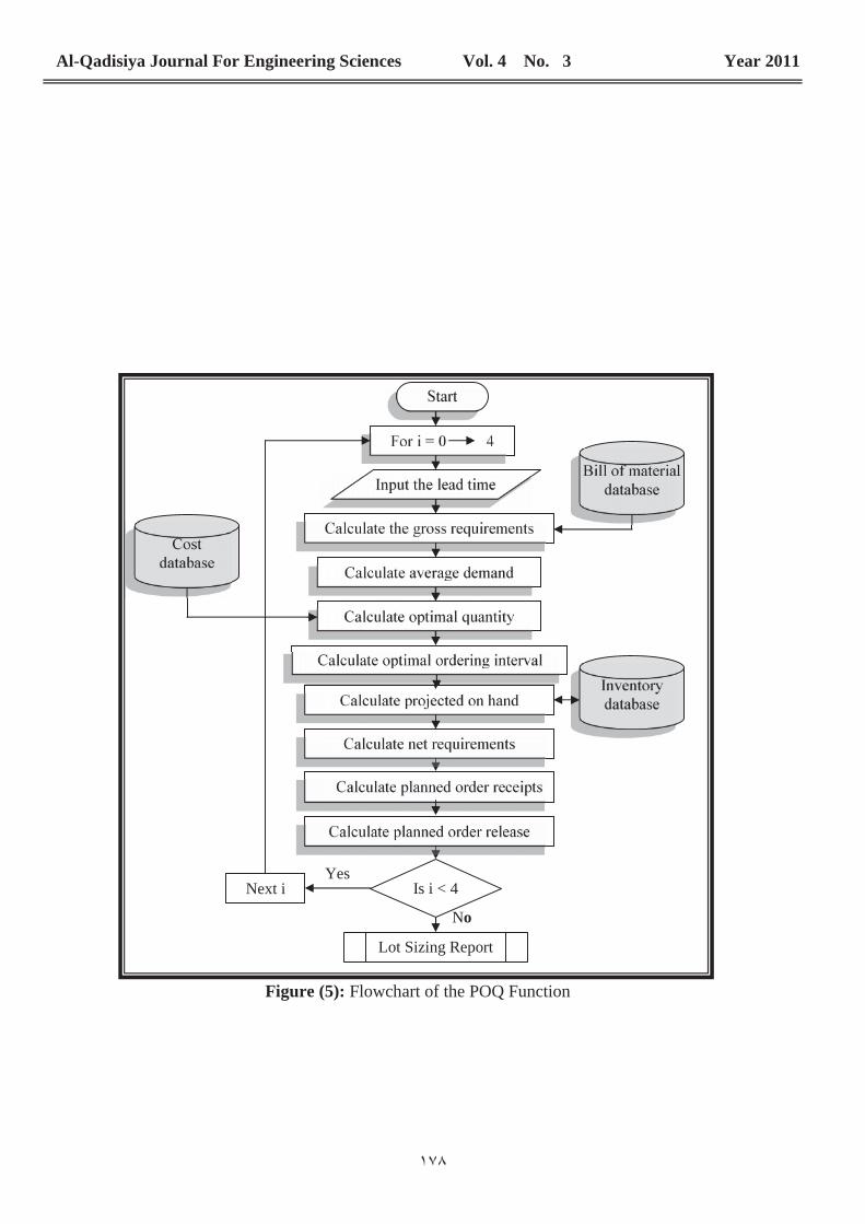
3. POQ Function: The periodic order quantity (POQ) technique is based on the same thinkingas the EOQ method. For the EOQ technique the order quantity is constant while orderinginterval varies. However, for the POQ model the ordering interval is constant while theorder quantity various, thus:

T=Q/D (2)

Where:T=Ordering interval.Q= Economic order quantity.D= Average demand for item per unit time.


The POQ function is built as shown in figure (5).

4. PPB Function: PPB is a more dynamic approach to balance setup and holding cost, PPBuses additional information by changing the lot size to reflect requirements of the next lotsize in the future. It divides demand requirements into order periods such that ordering andholding cost are balanced. Although the technique does not guarantee an optimum solution,it does produce a very good solution. The procedure for PPB is as follows:Calculate an economic part period or EPP, for the problem. This value is expressed as a ratiobetween ordering and holding cost. It is used as a measuring tool to determine when to placean order.

EPP = Ordering cost/ Carrying cost = Co/Cc (3)

This technique selects the order quantity at which the part period cost matches the EPPvalue, most closely

PPi= PPi-1 + (Ri*Ci) (4)

Where:PP: Cumulative Part-Period for period i.Ri: Requirement for period i.Ci: Duration for which inventory is carried.

The PPB function is built as shown in figure (6).5. WW function: The Wagner-Within procedure is a dynamic programming model that addssome complexity to the lot-size computation. Wagner-Within begins with the first period in theplanning horizon and evaluates all possible combinations of orders to meet demand in thatperiod. It then proceeds to period two and does the same, and so on, until the optimal methodfor meeting demand in all periods is determined.

The WW function is built as shown in figure (7).

4. RESULTS AND DISCUSSIONTo show the validity of our approach and for the purpose of completeness, we applied this

system in state company of rubber industries. This company provided us the necessary informationsuch as (production plan, ordering and carrying cost for product, operation time for all theproduction processes, and the inventory information). The company produces several types ofproducts. Product (X) is being selected which consists of (21) part. Planned order is released at thesame time for all the parts. The monthly quantity of product (X) are (1716) for September 2010.

The researcher selected part number (1) of product (X) to test the (CALS) system as follow:By entering the following data(current year, month, monthly quantity, days per period, and

holiday at each period), and by using the bill of material database that consist of(part number,quantity per assembly, and low level code). The cost database provide the system (ordering cost andcarrying cost). The inventory database provide the system (scheduled receipts, projected on handand lead time).the results are master production schedule table from the following equations:

Quantity per day= monthly quantity / number of work days during the month = 1716 / 26= 66Quantity per period= Quantity per day number of work days per period Quantity per period1 = 66 2 = 132Then the system calculate the lot sizing techniques as follow:1- Lot-for-lot:

{ Gross Requirements }= {Quantity per period} { Quantity per assembly } { Gross Requirements for period1}= 132 1 =132


{Net Requirements}= {Gross Requirements} {On-hand Inventory} {ScheduledReceipts}

{Net Requirements for period1}= 132 0 0=132{Planned Order Receipts}={Net Requirements}=132Total cost= Ordering cost for all period+ Carrying cost for all period = (8072.4 5)+ 0 = 40362 $

2- Economic order quantity:{ Gross Requirements }= {Quantity per period} { Quantity per assembly }

{ Gross Requirements for period1}= 132 1 =132Average demand for item per unit time(D)=SUM{ Gross Requirements for allperiods}/ number of periods= (132+396+396+396+396)/ 5=343.2

Economic order quantity (Q )= 2 Ordering cost per batch (S Average demandfor item per unit time(D) / Carrying cost per item per unit time(C)

Economic order quantity (Q )for period1= (2 8072.4 343.2) / 16.1448=586{Net Requirements}= {Gross Requirements} {On-hand Inventory} {ScheduledReceipts}

{Net Requirements for period1}= 132 0 0=132{Planned Order Receipts}={ Economic order quantity }=586Total cost= Ordering cost for all period+ Carrying cost for all period = (8072.4 4)+ (7329.7392+ 7329.7392+ 936.3984+0+9202.536)= 57088.0128 $

3- Periodic order quantity:{ Gross Requirements }= {Quantity per period} { Quantity per assembly }

{ Gross Requirements for period1}= 132 1 =132Average demand for item per unit time(D)=SUM{ Gross Requirements for allperiods}/ number of periods= (132+396+396+396+396)/ 5=343.2

Economic order quantity (Q )= 2 Ordering cost per batch (S Average demandfor item per unit time(D) / Carrying cost per item per unit time(C)

Economic order quantity (Q) for period1= (2 8072.4 343.2) / 16.1448=586Ordering interval(T)=Economic order quantity(Q)/Average demand for item per unittime(D) =586/343.2=2{Net Requirements}= {Gross Requirements} {On-hand Inventory} {ScheduledReceipts}

{Net Requirements for period1}= 132 0 0=132{Planned Order Receipts}={ Planned Order Receipts for pereiod1+ Planned OrderReceipts for pereiod2 }=132+396= 528

Total cost= Ordering cost for all period+ Carrying cost for all period = (8072.4 3)+ (6393.3408 2)= 37003.8816 $

4- Part-Period balancing:{ Gross Requirements }= {Quantity per period} { Quantity per assembly }

{ Gross Requirements for period1}= 132 1 =132Economic part period(EPP)=Ordering cost(Co)/Carrying cost(Cc)= 8072.4/16.1448=500Cumulative Part-Period for period 1 (PP1)= Cumulative Part-Period for period 0(PP0) + {Requirement for period 1 (R1)* Duration for which inventory is carried(C1)}

Cumulative Part-Period for period1(PP1)=0-(132 0)=0 (is this closet match to EPP)? No

{Prospective lot size for period 1 }={Net Requirements for period 1 + NetRequirements for period 0 }=132-0=132


Total cost= Ordering cost for all period+ Carrying cost for all period = (8072.4 4)+ (10655.568+4262.2272+6393.3408)= 53600.736$

5- Wagner-Within:{ Gross Requirements }= {Quantity per period} { Quantity per assembly }

{Gross Requirements for period1}= 132 1 =132{Net Requirements}= {Gross Requirements} {On-hand Inventory} {ScheduledReceipts}

{Net Requirements for period1}= 132 0 0=132

period alternatives Ordering cost Carrying cost Total cost Optimal policy1 (1) 8072.4 0 8072.4 (1)

After calculate all period the optimal policy is (1,2,3,4,5){Planned Order Receipts}=SUM{Net requirements}=132+396+396+396+396=1716Total cost= Ordering cost for all period+ Carrying cost for all period = (8072.4) +(25573.363+19180.022+12786.6811+6393.3408)= 72005.808$

From the above techniques the system selects the best technique (Periodic orderquantity) that have minimum cost

The application of the proposed system is introduced here.Figure (8) shows the proposed input frame and the result ( master production schedule

MPS) depend upon database in figure (9),(10),(11) to calculate the lot sizing technique for the fivetechniques as shows in figures (12),(13),(14),(15),(16).

Figure (17) shows the output of the system and the selected suitable lot sizing techniquedepend on minimum cost.

4. CONCLUSIONS In this paper, we construct a software program that selects the suitable lot sizing techniquedepend upon scientific bases.

The (CALS) system provides with bill of material database, inventory database, and costdatabase that can be updated at any time.

This model can be applied to solve lot sizing problems faster and easier because it can giveoptimum solution and posses certain characteristic that make the model more effective to be used.

From the (CALS) system we conclude the following:Lot-for-lot techniques order just what is required for production based on net requirements andit may not always be feasible. If setup costs are high, costs may be high as wellEOQ using average demand and expects a known constant demand and MRP systems often dealwith unknown and variable demandPart-period balancing tries to make the setup costs as close to the carrying costs as possible.Fixed order quantity method constant lot sizesWagner-Whitin

REFERENCEES[1] AL-Juboory, F.K., "Computer aided monitoring of production planning", M.Sc. thesis, Baghdad,2002.

[2] Cheng, T.C.E., " A Comparative study of some non-cost-based lot-sizing heuristics", ComputersInd. Engng. VOL. 16, No.1, PP87-96,1989, Pergamon Press PLC.

[3] De Matteis, J.J. and Mendoza, A.G., 1968. An economic lot sizing technique. IBM systemsJournal, 7: 30-


[4] Gaafar, L.K. and Choueiki, M.H., 2000, "A neural network model for solving the lot sizingproblem", The International Journal of Management Science, Omega. 28:175-184.

[5] Hoesel, Stan Van, and Wagelmans, Albert, " Sensitivity analysis of the economic lot-sizingproblem" OR 238-90 November 1990.

[6] Radzi,Nor Haizan Mohamed, Haron, Habibollah, and Johari ,Tuan Irdawati Tuan, " Lot SizingUsing Neural Network Approach" School of Mathematical Sciences, Universiti Sains Malaysia,Penang, June 13-15, 2006

[7] SAYDAM, CEM& EVANS, JAMES R., "A Comparative performance analysis of theWagner-Within algorithm and lot-sizing heuristics", Computers Ind. Engng. VOL. 18, No.1, PP.91-93,1990, Pergamon Press PLC.

Table (3): Lot Sizing Report

PeriodItem: LLC:

LS: LT:Current

1 2 3 4 5 6 7 8Gross Requirements

Scheduled Receipts

Projected InventoryBalance

Net Requirements

Planned orderReceipts

Planned OrderReleased

Item No. Projectedon Hand

Lead Time ScheduledReceipt

OrderingCost

HoldingCost

SerialNo.

PartNo.

LLC Quantity PerAssembly

Table (1): Item Master File

Table (2): Bill of Material File


WWfunction

Start

Enter your inputs

PPBfunction

POQfunction

EOQfunction

LFLfunction

Suitable Lot SizingTechnique

Figure (2): Flowchart of the Lot Sizing Module

Item MasterDatabase

Bill of MaterialDatabase

Figure (1): System architecture

User interface

Lot SizingModule

Common Database

Lot SizingReport


Start

For i = 0 4

Input the lead time

Calculate the gross requirements

Calculate projected on hand

Calculate net requirements

Calculate planned order release

Is I < 4

Lot Sizing ReportNo

YesNext i

Bill of materialdatabaseInventory

database

Figure (3): Flowchart of the LFL Function

Calculate planned order receipts

Start

For i = 0 4

Input the lead time


Calculate average demand

Calculate optimal quantity

Calculate net requirements (NR)

Is NR<= 4

Lot Sizing Report

No

Yes

Next i

Bill of materialdatabase

Costdatabase

Planned orderreceipts (POR1)=0

POR1= optimal quantity


Yes

NoIs i < 4

Inventorydatabase

Calculate planned order release (POR2)


Start

For i = 0 4

Input the lead time


Calculate average demand

Calculate optimal quantity

Calculate optimal ordering interval

Lot Sizing Report

Next i


Costdatabase

Figure (5): Flowchart of the POQ Function




Yes

No

Is i < 4

Inventorydatabase



Start

For i = 0 4

Input the lead time


Calculate economic part-period (EPP)



Lot Sizing Report

Next i


Costdatabase

Figure (6): Flowchart of the PPB Function

Calculate part-period (Cumulative)

Calculate prospective part-period

Calculate carried in inventory

Yes

No

Is i < 4

Inventorydatabase

Is PPC >EPPYes

No




Start

For i = 0 4

Input the lead time




Lot Sizing Report

Next i


Costdatabase

Figure (7): Flowchart of the WW Function

Select least total cost probability

Calculate Carrying cost

Calculate Probability

Yes

No

Is j < 4

Inventorydatabase

Is i < 4Yes

No



Calculate Ordering cost

For j = 0 4

Next j


Figure (8): The proposed input frame

Figure (9): Bill of Material Database frame

Figure (9): Cost Database frame

Figure (10): Cost Database frame


Figure (11): Inventory Database frame

Figure (12): Lot For Lot Technique Frame


Figure (14) Periodic Order Quantity Technique Frame

Figure (13) Economic Order Quantity Technique Frame


Figure (15) Part Period Balancing Technique Frame

Figure (16) Wagner -Within Algorithm Technique Frame


Figure (17) Select The Suitable Lot Size Technique Frame

computer-aided selection of the optimal...

Documents