chapter 1 mining time series datajessica/bookchaptertsmining.pdfchapter 1 mining time series data...

Chapter 1

MINING TIME SERIES DATA

Chotirat Ann Ratanamahatana, Jessica Lin, Dimitrios Gunopulos, EamonnKeoghUniversity of California, Riverside

Michail VlachosIBM T.J. Watson Research Center

Gautam DasUniversity of Texas, Arlington

Abstract Much of the world’s supply of data is in the form of time series. In the lastdecade, there has been an explosion of interest in mining time series data. Anumber of new algorithms have been introduced to classify, cluster, segment,index, discover rules, and detect anomalies/novelties in time series. While thesemany different techniques used to solve these problems use a multitude of differ-ent techniques, they all have one common factor; they require some high levelrepresentation of the data, rather than the original raw data. These high levelrepresentations are necessary as a feature extraction step, or simply to make thestorage, transmission, and computation of massive dataset feasible. A multitudeof representations have been proposed in the literature, including spectral trans-forms, wavelets transforms, piecewise polynomials, eigenfunctions, and sym-bolic mappings. This chapter gives a high-level survey of time series data miningtasks, with an emphasis on time series representations.

Keywords: Data Mining, Time Series, Representations, Classification, Clustering, Time Se-ries Similarity Measures

1. Introduction

Time series data accounts for an increasingly large fraction of the world’ssupply of data. A random sample of 4,000 graphics from 15 of the world’s

Ann Ratanamahatana

Text Box

PREVIEW VERSION

2

newspapers published from 1974 to 1989 found that more than 75% of allgraphics were time series (Tufte, 1983). Given the ubiquity of time series data,and the exponentially growing sizes of databases, there has been recently beenan explosion of interest in time series data mining. In the medical domainalone, large volumes of data as diverse as gene expression data (Aach andChurch, 2001), electrocardiograms, electroencephalograms, gait analysis andgrowth development charts are routinely created. Similar remarks apply toindustry, entertainment, finance, meteorology and virtually every other fieldof human endeavour. Although statisticians have worked with time series formore than a century, many of their techniques hold little utility for researchersworking with massive time series databases (for reasons discussed below).

Below are the major task considered by the time series data mining commu-nity.

Indexing (Query by Content): Given a query time seriesQ, and somesimilarity/dissimilarity measureD(Q,C), find the most similar time se-ries in databaseDB (Chakrabartiet al., 2002; Faloutsoset al., 1994;Kahveci and Singh, 2001; Popivanovet al., 2002).

Clustering: Find natural groupings of the time series in databaseDB un-der some similarity/dissimilarity measureD(Q,C) (Aach and Church,2001; Debregeas and Hebrail, 1998; Kalpakiset al., 2001; Keogh andPazzani, 1998).

Classification: Given an unlabeled time seriesQ, assign it to one of twoor more predefined classes (Geurts, 2001; Keogh and Pazzani, 1998).

Prediction (Forecasting): Given a time seriesQ containingn data points,predict the value at timen + 1.

Summarization: Given a time seriesQ containingn data points wheren is an extremely large number, create a (possibly graphic) approxima-tion of Q which retains its essential features but fits on a single page,computer screen, etc. (Indyket al., 2000; Wijk and Selow, 1999).

Anomaly Detection(Interestingness Detection): Given a time seriesQ,assumed to be normal, and an unannotated time seriesR, find all sectionsof R which contain anomalies or “surprising/interesting/unexpected” oc-currences (Guralnik and Srivastava, 1999; Keoghet al., 2002; Shahabiet al., 2000).

Segmentation: (a) Given a time seriesQ containingn data points, con-struct a modelQ, from K piecewise segments(K << n), such thatQ closely approximatesQ (Keogh and Pazzani, 1998). (b) Given a time

Mining Time Series Data 3

seriesQ, partition it intoK internally homogenous sections (also knownas change detection (Guralnik and Srivastava, 1999)).

Note that indexing and clustering makeexplicit use of a distance measure,and many approaches to classification, prediction, association detection, sum-marization, and anomaly detection makeimplicit use of a distance measure.We will therefore take the time to consider time series similarity in detail.

2. Time Series Similarity Measures

2.1 Euclidean Distances andLp Norms

One of the simplest similarity measures for time series is the Euclidean dis-tance measure. Assume that both time sequences are of the same lengthn, wecan view each sequence as a point inn-dimensional Euclidean space, and de-fine the dissimilarity between sequencesC andQ andD(C, Q) = Lp(C,Q),i.e. the distance between the two points measured by theLp norm (whenp = 2,it reduces to the familiar Euclidean distance). Figure 1.1 shows a visual intu-ition behind the Euclidean distance metric.

Figure 1.1. The intuition behind the Euclidean distance metric

Such a measure is simple to understand and easy to compute, which has en-sured that the Euclidean distance is the most widely used distance measure forsimilarity search (Agrawalet al., 1993; Chan and Fu, 1999; Faloutsoset al.,1994). However, one major disadvantage is that it is very brittle; it does not al-low for a situation where two sequences are alike, but one has been “stretched”or “compressed” in theY -axis. For example, a time series may fluctuate withsmall amplitude between 10 and 20, while another may fluctuate in a similarmanner with larger amplitude between 20 and 40. The Euclidean distance be-tween the two time series will be large. This problem can be dealt with easilywith offset translation and amplitude scaling, which requires normalizing thesequences before applying the distance operator1.

In Goldin and Kanellakis (1995) , the authors describe a method where thesequences are normalized in an effort to address the disadvantages of theLp asa similarity measure. Figure 1.2 illustrates the idea.

4

Figure 1.2. A visual intuition of the necessity to normalize time series before measuring thedistance between them. The two sequences Q and C appear to have approximately the sameshape, but have different offsets in Y-axis. The unnormalized data greatly overstate the sub-jective dissimilarity distance. Normalizing the data reveals the true similarity of the two timeseries.

More formally, letµ(C) andσ(C) be the mean and standard deviation ofsequenceC = {c1, . . . , cn}. The sequenceC is replaced by the normalizedsequencesC ′, where

c′i =ci − µ(C)

σ(C)Even after normalization, the Euclidean distance measure may still be un-

suitable for some time series domains since it does not allow for accelerationand deceleration along the time axis. For example, consider the two subjec-tively very similar sequences shown in Figure 1.3A. Even with normalization,the Euclidean distance will fail to detect the similarity between the two signals.This problem can generally be handled by Dynamic Time Warping distancemeasure, which will be discussed in the next section.

2.2 Dynamic Time Warping

In some time series domains, a very simple distance measure such as theEuclidean distance will suffice. However, it is often the case that the twosequences have approximately the same overall component shapes, but theseshapes do not line up inX-axis. Figure 1.3 shows this with a simple example.In order to find the similarity between such sequences or as a preprocessingstep before averaging them, we must “warp” the time axis of one (or both)sequences to achieve a better alignment. Dynamic Time Warping (DTW) is atechnique for effectively achieving this warping.

In Berndt and Clifford (1996) , the authors introduce the technique of dy-namic time warping to the data mining community. Dynamic time warping is


Figure 1.3. Two time series which require a warping measure. Note that while the sequenceshave an overall similar shape, they are not aligned in the time axis. Euclidean distance, whichassumes theith point on one sequence is aligned withith point on the other (A), will producea pessimistic dissimilarity measure. A nonlinear alignment (B) allows a more sophisticateddistance measure to be calculated.

an extensively used technique in speech recognition, and allows acceleration-deceleration of signals along the time dimension. We describe the basic ideabelow.

Consider two sequence (of possibly different lengths),C = {c1, . . . ,cm} andQ = {q1, . . . ,qn}. When computing the similarity of the two time series usingDynamic Time Warping, we are allowed to extend each sequence by repeatingelements.

A straightforward algorithm for computing the Dynamic Time Warping dis-tance between two sequences uses a bottom-up dynamic programming ap-proach, where the smaller sub-problemsD(i, j) are first determined, and thenused to solve the larger sub-problems, untilD(m, n) is finally achieved, asillustrated in Figure 1.4 below.

Figure 1.4. A) Two similar sequences Q and C, but out of phase. B) To align the sequences, weconstruct a warping matrix, and search for the optimal warping path, shown with solid squares.Note that the “corners” of the matrix (shown in dark gray) are excluded from the search path(specified by a warping window of size w) as part of an Adjustment Window condition. C) Theresulting alignment

Although this dynamic programming technique is impressive in its abilityto discover the optimal of an exponential number alignments, a basic imple-mentation runs inO(mn) time. If a warping windoww is specified, as shown

6

in Figure 1.4B, then the running time reduces toO(nw), which is still tooslow for most large scale application. In (Ratanamahatana and Keogh, 2004),the authors introduce a novel framework based on a learned warping windowconstraint to further improve the classification accuracy, as well as to speed upthe DTW calculation by utilizing the lower bounding technique introduced in(Keogh, 2002).

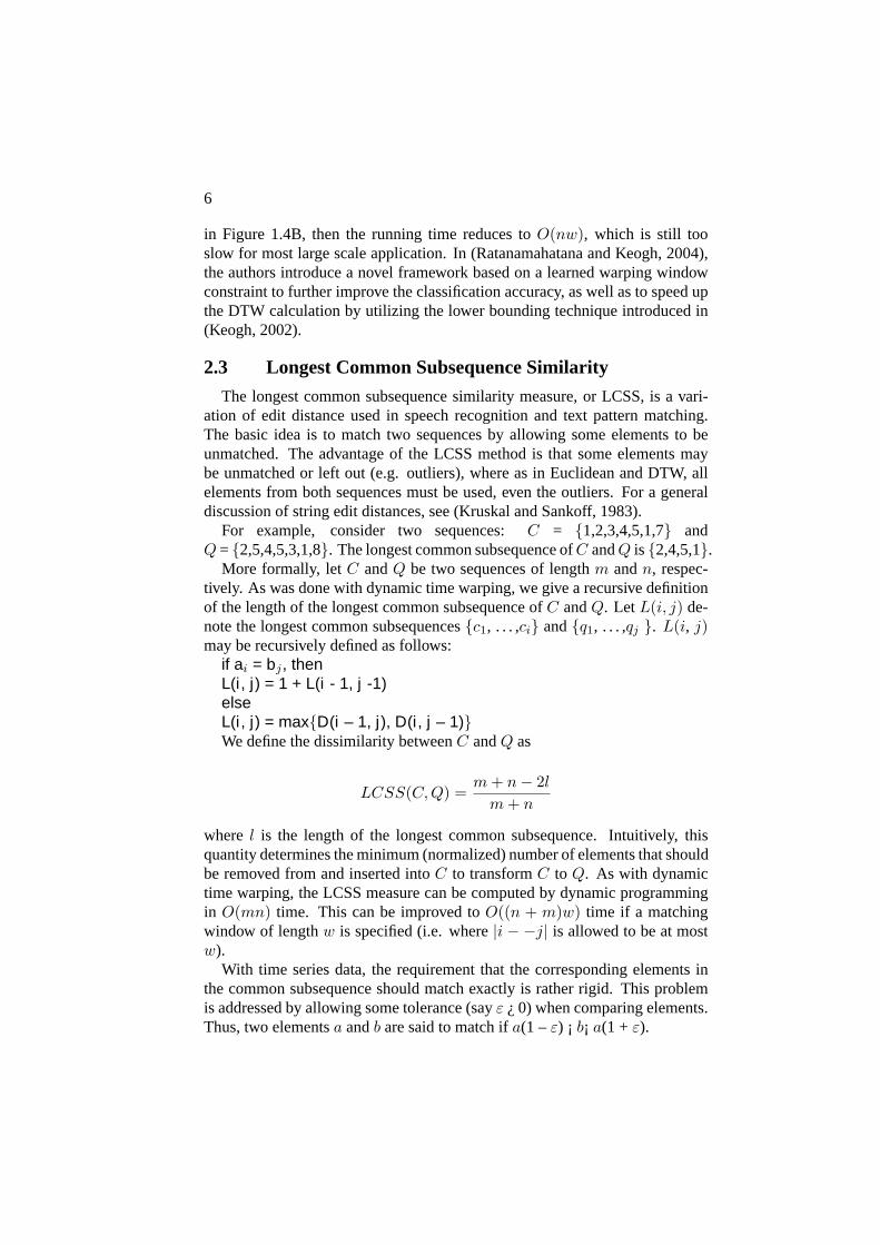
2.3 Longest Common Subsequence Similarity

The longest common subsequence similarity measure, or LCSS, is a vari-ation of edit distance used in speech recognition and text pattern matching.The basic idea is to match two sequences by allowing some elements to beunmatched. The advantage of the LCSS method is that some elements maybe unmatched or left out (e.g. outliers), where as in Euclidean and DTW, allelements from both sequences must be used, even the outliers. For a generaldiscussion of string edit distances, see (Kruskal and Sankoff, 1983).

For example, consider two sequences:C = {1,2,3,4,5,1,7} andQ = {2,5,4,5,3,1,8}. The longest common subsequence ofC andQ is{2,4,5,1}.

More formally, letC andQ be two sequences of lengthm andn, respec-tively. As was done with dynamic time warping, we give a recursive definitionof the length of the longest common subsequence ofC andQ. Let L(i, j) de-note the longest common subsequences{c1, . . . ,ci} and{q1, . . . ,qj }. L(i, j)may be recursively defined as follows:

if ai = bj , thenL(i , j) = 1 + L(i - 1, j -1)elseL(i , j) = max{D(i – 1, j), D(i , j – 1)}We define the dissimilarity betweenC andQ as

LCSS(C, Q) =m + n− 2l

m + n

where l is the length of the longest common subsequence. Intuitively, thisquantity determines the minimum (normalized) number of elements that shouldbe removed from and inserted intoC to transformC to Q. As with dynamictime warping, the LCSS measure can be computed by dynamic programmingin O(mn) time. This can be improved toO((n + m)w) time if a matchingwindow of lengthw is specified (i.e. where|i − −j| is allowed to be at mostw).

With time series data, the requirement that the corresponding elements inthe common subsequence should match exactly is rather rigid. This problemis addressed by allowing some tolerance (sayε ¿ 0) when comparing elements.Thus, two elementsa andb are said to match ifa(1 –ε) ¡ b¡ a(1 + ε).


In the next two subsections, we discuss approaches that try to incorporatelocal scaling and global scaling functions in the basic LCSS similarity measure.

2.3.1 Using local Scaling Functions. In (Agrawalet al., 1995), theauthors develop a similarity measure that resembles LCSS-like similarity withlocal scaling functions. Here, we only give an intuitive outline of the complexalgorithm; further details may be found in the paper.

The basic idea is that two sequences are similar if they have enough non-overlapping time-ordered pairs of contiguous subsequences that are similar.Two contiguous subsequences are similar if one can be scaled and translatedappropriately to approximately resemble the other. The scaling and translationfunction is local, i.e. it may be different for other pairs of subsequences.

The algorithmic challenge is to determine how and where to cut the originalsequences into subsequences so that the overall similarity is minimized. Wedescribe it briefly here (refer to (Agrawalet al., 1995) for further details). Thefirst step is to find all pairs of atomic subsequences in the original sequencesA andQ that are similar (atomic implies subsequences of a certain small size,say a parameterw). This step is done by a spatial self-join (using a spatialaccess structure such as an R-tree) over the set of all atomic subsequences.The next step is to “stitch” similar atomic subsequences to form pairs of largersimilar subsequences. The last step is to find a non-overlapping ordering ofsubsequence matches having the longest match length. The stitching and sub-sequence ordering steps can be reduced to finding longest paths in a directedacyclic graph, where vertices are pairs of similar subsequences, and a directededge denotes their ordering along the original sequences.

2.3.2 Using a global scaling function. Instead of different local scal-ing functions that apply to different portions of the sequences, a simpler ap-proach is to try and incorporate a single global scaling function with the LCSSsimilarity measure. An obvious method is to first normalize both sequencesand then apply LCSS similarity to the normalized sequences. However, thedisadvantage of this approach is that the normalization function is derived fromall data points, including outliers. This defeats the very objective of the LCSSapproach which is to ignore outliers in the similarity calculations.

In (Bollobaset al., 2001), an LCSS-like similarity measure is described thatderives a global scaling and translation function that is independent of outliersin the data. The basic idea is that two sequencesC andQ are similar if thereexists constantsa andb, and long common subsequencesC ′ andQ′ such thatQ′ is approximately equal toaC’ + b. The scale+translation linear function(i.e. the constantsa andb) is derived from the subsequences, and not from theoriginal sequences. Thus, outliers cannot taint the scale+translation function.

8

Although it appears that the number of all linear transformations is infinite,Bollobaset al. (2001) shows that the number of different unique linear trans-formations isO(n2). A naive implementation would be to compute LCSS onall transformations, which would lead to an algorithm that takesO(n3) time.Instead, in (Bollobaset al., 2001), an efficient randomized approximation al-gorithm is proposed to compute this similarity.

2.4 Probabilistic methods

A different approach to time-series similarity is the use of a probabilis-tic similarity measure. Such measures have been studied in (Ge and Smyth,2000; Keogh and Smyth, 1997). While previous methods were “distance”based, some of these methods are “model” based. Since time series similar-ity is inherently a fuzzy problem, probabilistic methods are well suited forhandling noise and uncertainty. They are also suitable for handling scaling andoffset translations. Finally, they provide the ability to incorporate prior knowl-edge into the similarity measure. However, it is not clear whether other prob-lems such as time-series indexing, retrieval and clustering can be efficientlyaccomplished under probabilistic similarity measures.

Here, we briefly describe the approach in (Ge and Smyth, 2000). Givena sequenceC, the basic idea is to construct a probabilistic generative modelMC , i.e. a probability distribution on waveforms. Once a modelMC has beenconstructed for a sequenceC, we can compute similarity as follows. Given anew sequence patternQ, similarity is measured by computingp(Q|MC), i.e.the likelihood thatMC generatesQ.

2.5 General Transformations

Recognizing the importance of the notion of “shape” in similarity computa-tions, an alternate approach was undertaken by Jagadishet al. (1995) . In thispaper, the authors describe a general similarity framework involving a trans-formation rules language. Each rule in the transformation language takes aninput sequence and produces an output sequence, at a cost that is associatedwith the rule. The similarity of sequenceC to sequenceQ is the minimumcost of transformingC to Q by applying a sequence of such rules. The actualrules language is application specific.

3. Time Series Data Mining

The last decade has seen the introduction of hundreds of algorithms to clas-sify, cluster, segment and index time series. In addition, there has been muchwork on novel problems such as rule extraction, novelty discovery, and depen-dency detection. This body of work draws on the fields of statistics, machinelearning, signal processing, information retrieval, and mathematics. It is in-


teresting to note that with the exception of indexing, researches in the tasksenumerated above predate not only the decade old interest in data mining, butin computing itself. What then, are the essential differences between the classicand the data mining versions of these problems? The key difference is simplyone of size and scalability; time series data miners routinely encounter datasetsthat are gigabytes in size. As a simple motivating example, consider hierarchi-cal clustering. The technique has a long history and well-documented utility.If however, we wish to hierarchically cluster a mere million items, we wouldneed to construct a matrix with1012 cells, well beyond the abilities of the av-erage computer for many years to come. A data mining approach to clusteringtime series, in contrast, must explicitly consider the scalability of the algorithm(Kalpakiset al., 2001).

In addition to the large volume of data, most classic machine learning anddata mining algorithms do not work well on time series data due to their uniquestructure; it is often the case that each individual time series has a very high di-mensionality, high feature correlation, and large amount of noise (Chakrabartiet al., 2002), which present a difficult challenge in time series data miningtasks. Whereas classic algorithms assume relatively low dimensionality (forexample, a few measurements such as “height, weight, blood sugar, etc.”),time series data mining algorithms must be able to deal with dimensionalitiesin the hundreds or thousands. The problems created by high dimensional dataare more than mere computation time considerations; the very meanings ofnormally intuitive terms such as “similar to” and “cluster forming” become un-clear in high dimensional space. The reason is that as dimensionality increases,all objects become essentially equidistant to each other, and thus classificationand clustering lose their meaning. This surprising result is known as the “curseof dimensionality” and has been the subject of extensive research (Aggarwalet al., 2001). The key insight that allows meaningful time series data miningis that although the actual dimensionality may be high, theintrinsic dimen-sionality is typically much lower. For this reason, virtually all time series datamining algorithms avoid operating on the original “raw” data; instead, theyconsider some higher-level representation or abstraction of the data.

Before giving a full detail on time series representations, we first briefly ex-plore some of the classic time series data mining tasks. While these individualtasks may be combined to obtain more sophisticated data mining applications,we only illustrate their main basic ideas here.

3.1 Classification

Classification is perhaps the most familiar and most popular data miningtechnique. Examples of classification applications include image and patternrecognition, spam filtering, medical diagnosis, and detecting malfunctions in

10

industry applications. Classification maps input data into predefined groups. Itis often referred to as supervised learning, as the classes are determined priorto examining the data; a set of predefined data is used in training process andlearn to recognize patterns of interest. Pattern recognition is a type of classifi-cation where an input pattern is classified into one of several classes based onits similarity to these predefined classes. Two most popular methods in timeseries classification include the Nearest Neighbor classifier and Decision trees.Nearest Neighbor method applies the similarity measures to the object to beclassified to determine its best classification based on the existing data that hasalready been classified. For decision tree, a set of rules are inferred from thetraining data, and this set of rules is then applied to any new data to be classi-fied. Note that even though decision trees are defined for real data, attemptingto apply raw time series data could be a mistake due to its high dimensionalityand noise level that would result in deep, bushy tree. Instead, some researcherssuggest representing time series as Regression Tree to be used in Decision Treetraining (Geurts, 2001).

The performance of classification algorithms is usually evaluated by mea-suring the accuracy of the classification, by determining the percentage of ob-jects identified as the correct class.

3.2 Indexing (Query by Content)

Query by content in time series databases has emerged as an area of ac-tive interest since the classic first paper by Agrawal et al. (1993) . This alsoincludes a sequence matching task which has long been divided into two cat-egories: whole matching and subsequence matching (Faloutsoset al., 1994;Keoghet al., 2001).

Whole Matching: a query time series is matched against a database ofindividual time series to identify the ones similar to the query

Subsequence Matching: a short query subsequence time series is matchedagainst longer time series by sliding it along the longer sequence, looking forthe best matching location.

While there are literally hundreds of methods proposed for whole sequencematching (See, e.g. (Keogh and Kasetty, 2002) and references therein), inpractice, its application is limited to cases where some information about thedata is knowna priori.

Subsequence matching can be generalized to whole matching by dividingsequences into non-overlapping sections by either a specific period or, morearbitrarily, by its shape. For example, we may wish to take a long electro-cardiogram and extract the individual heartbeats. This informal idea has beenused by many researchers.


Most of the indexing approaches so far use the original GEMINI framework(Faloutsoset al., 1994) but suggest a different approach to the dimensionalityreduction stage. There is increasing awareness that for many data mining andinformation retrieval tasks, very fast approximate search is preferable to slowerexact search (Changet al., 2002). This is particularly true for exploratorypurposes and hypotheses testing. Consider the stock market data. While itmakes sense to look for approximate patterns, for example, “a pattern thatrapidly decreases after a long plateau”, it seems pedantic to insist onexactmatches. Next we would like to discuss similarity search in some more detail.

Given a database of sequences, the simplest way to find the closest matchto a given query sequenceQ, is to perform alinear or sequentialscan of thedata. Each sequence is retrieved from disk and its distance to the queryQis calculated according to the pre-selected distance measure. After the querysequence is compared to all the sequences in the database, the one with thesmallest distance is returned to the user as the closest match.

This brute-force technique is costly to implement, first because it requiresmany accesses to the disk and second because it operates or the raw sequences,which can be quite long. Therefore, the performance of linear scan on the rawdata is typically very costly.

A more efficient implementation of the linear scan would be to store twolevels of approximation of the data; the raw data and their compressed version.Now the linear scan is performed on the compressed sequences and alowerboundto the original distance is calculated for all the sequences. The raw dataare retrieved in the order suggest by the lower bound approximation of theirdistance to the query. The smallest distance to the query is updated after eachraw sequence is retrieved. The search can be terminated when the lower boundof the currently examined object exceeds the smallest distance discovered sofar.

A more efficient way to perform similarity search is to utilize anindexstructurethat will cluster similar sequences into the same group, hence pro-viding faster access to the most promising sequences. Using various pruningtechniques, indexing structures can avoid examining large parts of the dataset,while still guaranteeing that the results will be identical with the outcome oflinear scan. Indexing structures can be divided into two major categories: vec-tor based and metric based.

3.2.1 Vector Based Indexing Structures. Vector based indices workon the compressed data dimensionality. The original sequences are compactedusing a dimensionality reduction method, and the resulting multi-dimensionalvectors can be grouped into similar clusters using some vector-based indexingtechnique, as shown in Figure 1.5.

12

Figure 1.5. Dimensionality reduction of time-series into two dimensions

Vector-based indexing structures can also appear in two flavors; hierarchicalor non-hierarchical. The most common hierarchical vector based index is theR-tree or some variants. The R-tree consists of multi-dimensional vector onthe leaf levels, which are organized in the tree fashion using hyper-rectanglesthat can potentially overlap, as illustrated in Figure 1.6.

In order to perform the search using an index structure, the query is also pro-jected in the compressed dimensionality and then probed on the index. Usingthe R-tree, only neighboring hyper-rectangles to the query’s projected locationneed to be examined.

Other commonly used hierarchical vector-based indices are the kd-B-trees(Robinson, 1981) and the quad-trees (Tufte, 1983). Non-hierarchical vectorbased structures are less common and are typically known as grid files (Niev-ergeltet al., 1984). For example, grid files have been used in (Zhu and Shasha,2002) for the discovery of the most correlated data sequences.

However, such types of indexing structures work well only for low com-pressed dimensionalities (typically¡5). For higher dimensionalities, the prun-ing power of vector-based indices diminishes exponentially. This can be exper-imentally and analytically shown and it is coined under the term ‘dimension-ality curse’ (Zhu and Shasha, 2002). This inescapable fact suggests that evenwhen using an index structure, the complete dataset would have to be retrievedfrom disk for higher compressed dimensionalities.

3.2.2 Metric Based Indexing Structures. Metric based structurescan typically perform much better than vector based indices, even for higherdimensionalities (up to 20 or 30). They are more flexible because they require


Figure 1.6. Hierarchical organization using an R-tree

only distances between objects. Thus, they do not cluster objects based ontheir compressed features but based on relative object distances. The choice ofreference objects, from which all object distances will be calculated, can varyin different approaches. Examples of metric trees include the Vantage Point(VP) tree (Yianilos, 1992), M-tree (Ciacciaet al., 1997) and GNAT (Brin,1995). All variations of such trees, exploit the distances to the reference pointsin conjunction with the triangle inequality to prune parts of the tree, where nocloser matches (to the ones already discovered) can be found. A recent useof VP-trees for time-series search under Euclidean distance using compressedFourier descriptors can be found in (Vlachoset al., 2004).

3.3 Clustering

Clustering is similar to classification that categorizes data into groups; how-ever, these groups are not predefined, but rather defined by the data itself, basedon the similarity between time series. It is often referred to as unsupervisedlearning. The clustering is usually accomplished by determining the similarityamong the data on predefined attributes. The most similar data are groupedinto clusters, but the clusters themselves should be very dissimilar. And sincethe clusters are not predefined, a domain expert is often required to interpretthe meaning of the created clusters. The two general methods of time seriesclustering are Partitional Clustering and Hierarchical Clustering. HierarchicalClustering computes pairwise distance, and then merges similar clusters in a

14

bottom-up fashion, without the need of providing the number of clusters. Webelieve that this is one of the best (subjective) tools to data evaluation, by cre-ating a dendrogram of several time series from the domain of interest (Keoghand Pazzani, 1998), as shown in Figure 1.7. However, its application is limitedto only small datasets due to its quadratic computational complexity.

Figure 1.7. A hierarchical clustering of time series

On the other hand, Paritional Clustering typically uses theK-means algo-rithm (or some variant) to optimize the objective function by minimizing thesum of squared intra-cluster errors. While the algorithm is perhaps the mostcommonly used clustering algorithm in the literature, one of its shortcomingsis the fact that the number of clusters,K, must be pre-specified.

Clustering has been used in many application domains including biology,medicine, anthropology, marketing, and economics. It is also a vital processfor condensing and summarizing information, since it can provide a synop-sis of the stored data. Similar to query by content, there are two types oftime series clustering: whole clustering and subsequence clustering. The no-tion of whole clustering is similar to that of conventional clustering of discreteobjects. Given a set of individual time series data, the objective is to groupsimilar time series into the same cluster. On the other hand, given a single(typically long) time series, subsequence clustering is performed on each in-dividual time series (subsequence) extracted from the long time series with asliding window. Subsequence clustering is a common pre-processing step formany pattern discovery algorithms, of which the most well-known being theone proposed for time series rule discovery. Recent empirical and theoreticalresults suggest that subsequence clustering may not be meaningful on an entiredataset (Keoghet al., 2003), and that clustering should only be applied to asubset of the data. Some feature extraction algorithm must choose the subsetof data, but we cannot use clustering as the feature extraction algorithm, as thiswould open the possibility of a chicken and egg paradox. Several researchers


have suggested using time series motifs (see below) as the feature extractionalgorithm (Chiuet al., 2003).

3.4 Prediction (Forecasting)

Prediction can be viewed as a type of clustering or classification. The dif-ference is that prediction is predicting a future state, rather than a current one.Its applications include obtaining forewarning of natural disasters (flooding,hurricane, snowstorm, etc), epidemics, stock crashes, etc. Many time seriesprediction applications can be seen in economic domains, where a predictionalgorithm typically involves regression analysis. It uses known values of datato predict future values based on historical trends and statistics. For exam-ple, with the rise of competitive energy markets, forecasting of electricity hasbecome an essential part of an efficient power system planning and operation.This includes predicting future electricity demands based on historical data andother information, e.g. temperature, pricing, etc. As another example, the salesvolume of cellular phone accessories can be forecasted based on the number ofcellular phones sold in the past few months. Many techniques have been pro-posed to increase the accuracy of time series forecast, including the use neuralnetwork and dimensionality reduction techniques.

3.5 Summarization

Since time series data can be massively long, a summarization of the datamay be useful and necessary. A statistic summarization of the data, such asthe mean or other statistical properties can be easily computed even thoughit might not be particularly valuable or intuitive information. Rather, we canoften utilize natural language, visualization, or graphical summarization to ex-tract useful or meaningful information from the data. Anomaly detection andmotif discovery (see the next section below) are special cases of summarizationwhere only anomalous/repeating patterns are of interest and reported. Summa-rization can also be viewed as a special type of clustering problem that mapsdata into subsets with associated simple (text or graphical) descriptions andprovides a higher-level view of the data. This new simpler description of thedata is then used in place of the entire dataset. The summarization may be doneat multiple granularities and for different dimensions.

Some of popular approaches for visualizing massive time series datasetsincludeTimeSearcher, Calendar-Based Visualization, SpiralandVizTree.

TimeSearcher(Hochheiser and Shneiderman, 2001) is a query-by-exampletime series exploratory and visualization tool that allows user to retrieve timeseries by creating queries, so called TimeBoxes. Figure 1.8 shows three Time-Boxes being drawn to specify time series that start low, increase, then fall once

16

more. However, some knowledge about the datasets may be needed in advanceand users need to have a general idea of what to look for or what is interesting.

Figure 1.8. The TimeSearcher visual query interface. A user can filter away sequences thatare not interesting by insisting that all sequences have at least one data point within the queryboxes

Cluster and Calendar-Based Visualization(Wijk and Selow, 1999) is a visu-alization system that ‘chunks’ time series data into sequences of day patterns,and these day patterns are clustered using a bottom-up clustering algorithm.The system displays patterns represented by cluster average, along with a cal-endar with each day color-coded by the cluster it belongs to. Figure 1.9 showsan example view of this visualization scheme. From viewing patterns whichare linked to a calendar we can potentially discover simple rules such as: “Inthe winter months the power consumption is greater than in summer months”.

Spiral (Weberet al., 2000) maps each periodic section of time series ontoone “ring” and attributes such as color and line thickness are used to charac-terize the data values. The main use of the approach is the identification of


Figure 1.9. The cluster and calendar-based visualization on employee working hours data. Itshows six clusters, representing different working-day pattern

periodic structures in the data. Figure 1.10 displays the annual power usagethat characterizes the normal “9-to-5” working week pattern. However, theutility of this tool is limited for time series that do not exhibit periodic behav-iors, or when the period is unknown.

Figure 1.10. The Spiral visualization approach applied to the power usage dataset

VizTree(Lin et al., 2004) is recently introduced with the aim to discoverpreviouslyunknownpatterns with little or no knowledge about the data; it pro-vides an overall visual summary, and potentially reveal hidden structures in the

18

data. This approach first transforms the time series into a symbolic representa-tion, and encodes the data in a modified suffix tree in which the frequency andother properties of patterns are mapped onto colors and other visual properties.Note that even though the tree structure needs the data to be discrete, the origi-nal time series data is not. Using a time-series discretization introduced in (Linet al., 2003), continuous data can be transformed into discrete domain, withcertain desirable properties such as lower-bounding distance, dimensionalityreduction, etc. While frequently occurring patterns can be detected by thickbranches in VizTree, simple anomalous patterns can be detected by unusu-ally thin branches. Figure 1.11 demonstrates both motif discovery and simpleanomaly diction on ECG data.

Figure 1.11. ECG data with anomaly is shown. While the subsequence tree can be used toidentify motifs, it can be used for simple anomaly detection as well

3.6 Anomaly Detection

In time series data mining and monitoring, the problem of detecting anoma-lous/surprising/novel patterns has attracted much attention (Dasgupta and For-rest, 1999; Ma and Perkins, 2003; Shahabiet al., 2000). In contrast to subse-quence matching, anomaly detection is identification of previouslyunknownpatterns. The problem is particularly difficult because what constitutes ananomaly can greatly differ depending on the task at hand. In a general sense, ananomalous behavior is one that deviates from “normal” behavior. While therehave been numerous definitions given fro anomalous or surprising behaviors,


the one given by (Keoghet al., 2002) is unique in that it requires no ex-plicit formulation of what is anomalous. Instead, the authors simply define ananomalous pattern as on “whose frequency of occurrences differs substantiallyfrom that expected, given previously seen data”. The problem of anomaly de-tection in time series has been generalized to include the detection of surprisingor interesting patterns (which are not necessarily anomalies). Anomaly detec-tion is closely related to Summarization, as discussed in the previous section.Figure 1.12 illustrates the idea.

Figure 1.12. An example of anomaly detection from the MIT-BIH Noise Stress Test Database.Here, we show only a subsection containing the two most interesting events detected by thecompression-based algorithm (Keogh et al., 2004) (the thicker the line, the more interestingthe subsequence). The gray markers are independent annotations by a cardiologist indicatingPremature Ventricular Contractions.

3.7 Segmentation

Segmentation in time series is often referred to as a dimensionality reduc-tion algorithm. Although the segments created could be polynomials of anarbitrary degree, the most common representation of the segments is of linearfunctions. Intuitively, a Piecewise Linear Representation (PLR) refers to theapproximation of a time seriesQ, of lengthn, with K straight lines. Figure1.13 contains an example.

Figure 1.13. An example of a time series segmentation with its piecewise linear representation

BecauseK is typically much smaller thann, this representation makes thestorage, transmission, and computation of the data more efficient.

20

Although appearing under different names and with slightly different im-plementation details, most time series segmentation algorithms can be groupedinto one of the following three categories.

Sliding-Windows (SW): A segment is grown until it exceeds some errorbound. The process repeats with the next data point not included in thenewly approximated segment.

Top-Down (TD): The time series is recursively partitioned until somestopping criteria is met.

Bottom-Up (BU): Starting from the finest possible approximation, seg-ments are merged until some stopping criteria are met.

We can measure the quality of a segmentation algorithm in several ways, themost obvious of which is to measure the reconstruction error for a fixed numberof segments. The reconstruction error is simply the Euclidean distance betweenthe original data and the segmented representation. While most work in thisarea has consider static cases, recently researchers have consider obtaining andmaintaining segmentations on streaming data sources (Palpanaset al., 2004)

4. Time Series Representations

As noted in the previous section, time series datasets are typically very large,for example, just eight hours of electroencephalogram data can require in ex-cess of a gigabyte of storage. Rather than analyzing or finding statistical prop-erties on time series data, time series data miners’ goal is more towards discov-ering useful information from the massive amount of data efficiently. This is aproblem because for almost all data mining tasks, most of the execution timespent by algorithm is used simply to move data from disk into main memory.This is acknowledged as the major bottleneck in data mining because manynaıve algorithms require multiple accesses of the data. As a simple example,imagine we are attempting to dok-means clustering of a dataset that does notfit into main memory. In this case, every iteration of the algorithm will requirethat data in main memory to be swapped. This will result in an algorithm thatis thousands of times slower than the main memory case.

With this in mind, a generic framework for time series data mining hasemerged. The basic idea can be summarized as follows.

As with most problems in computer science, the suitable choice of represen-tation/approximation greatly affects the ease and efficiency of time series datamining. It should be clear that the utility of this framework depends heavilyon the quality of the approximation created in Step 1). If the approximationis very faithful to the original data, then the solution obtained in main mem-ory is likely to be the same as, or very close to, the solution we would haveobtained on the original data. The handful of disk accesses made in Step 2)


Table 1.1. A generic time series data mining approach.

1) Create an approximation of the data, which will fit in main memory, yet retainsthe essential features of interest.

2) Approximately solve the problem at hand in main memory.3) Make (hopefully very few) accesses to the original data on disk to confirm

the solution obtained in Step 2, or to modify the solution so it agrees with thesolution we would have obtained on the original data.

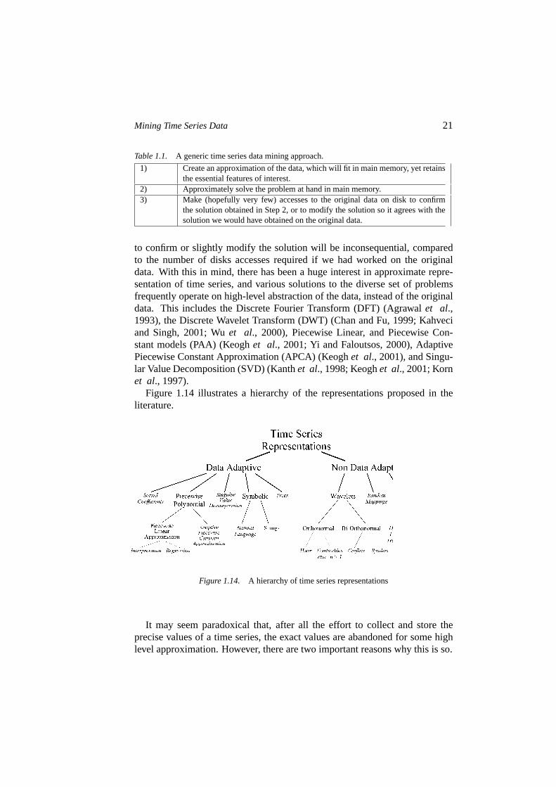
to confirm or slightly modify the solution will be inconsequential, comparedto the number of disks accesses required if we had worked on the originaldata. With this in mind, there has been a huge interest in approximate repre-sentation of time series, and various solutions to the diverse set of problemsfrequently operate on high-level abstraction of the data, instead of the originaldata. This includes the Discrete Fourier Transform (DFT) (Agrawalet al.,1993), the Discrete Wavelet Transform (DWT) (Chan and Fu, 1999; Kahveciand Singh, 2001; Wuet al., 2000), Piecewise Linear, and Piecewise Con-stant models (PAA) (Keoghet al., 2001; Yi and Faloutsos, 2000), AdaptivePiecewise Constant Approximation (APCA) (Keoghet al., 2001), and Singu-lar Value Decomposition (SVD) (Kanthet al., 1998; Keoghet al., 2001; Kornet al., 1997).

Figure 1.14 illustrates a hierarchy of the representations proposed in theliterature.

Figure 1.14. A hierarchy of time series representations

It may seem paradoxical that, after all the effort to collect and store theprecise values of a time series, the exact values are abandoned for some highlevel approximation. However, there are two important reasons why this is so.

22

We are typically not interested in the exact values of each time series datapoint. Rather, we are interested in the trends, shapes and patterns containedwithin the data. These may best be captured in some appropriate high-levelrepresentation.

As a practical matter, the size of the database may be much larger than wecan effectively deal with. In such instances, some transformation to a lowerdimensionality representation of the data may allow more efficient storage,transmission, visualization, and computation of the data.

While it is clear no one representation can be superior for all tasks, theplethora of work on mining time series has not produced any insight into howone should choose the best representation for the problem at hand and data ofinterest. Indeed the literature is not even consistent on nomenclature. For ex-ample, one time series representation appears under the names Piecewise FlatApproximation (Faloutsoset al., 1997), Piecewise Constant Approximation(Keoghet al., 2001) and Segmented Means (Yi and Faloutsos, 2000).

To develop the reader’s intuition about the various time series representa-tions, we have discussed and illustrated some of the well-known representa-tions in the following subsections below.

4.1 Discrete Fourier Transform

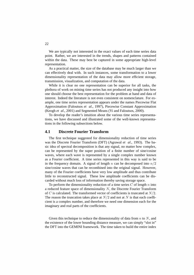
The first technique suggested for dimensionality reduction of time serieswas the Discrete Fourier Transform (DFT) (Agrawalet al., 1993). The ba-sic idea of spectral decomposition is that any signal, no matter how complex,can be represented by the super position of a finite number of sine/cosinewaves, where each wave is represented by a single complex number knownas a Fourier coefficient. A time series represented in this way is said to bein the frequency domain. A signal of lengthn can be decomposed inton/2sine/cosine waves that can be recombined into the original signal. However,many of the Fourier coefficients have very low amplitude and thus contributelittle to reconstructed signal. These low amplitude coefficients can be dis-carded without much loss of information thereby saving storage space.

To perform the dimensionality reduction of a time seriesC of lengthn intoa reduced feature space of dimensionalityN , the Discrete Fourier Transformof C is calculated. The transformed vector of coefficients is truncated atN/2.The reason the truncation takes place atN/2 and not atN is that each coeffi-cient is a complex number, and therefore we need one dimension each for theimaginary and real parts of the coefficients.

Given this technique to reduce the dimensionality of data fromn to N , andthe existence of the lower bounding distance measure, we can simply “slot in”the DFT into the GEMINI framework. The time taken to build the entire index


Figure 1.15. A visualization of the DFT dimensionality reduction technique

depends on the length of the queries for which the index is built. When thelength is an integral power of two, an efficient algorithm can be employed.

This approach, while initially appealing, does have several drawbacks. Noneof the implementations presented thus far can guarantee no false dismissals.Also, the user is required to input several parameters, including the size of thealphabet, but it is not obvious how to choose the best (or even reasonable) val-ues for these parameters. Finally, none of the approaches suggested will scalevery well to massive data since they require clustering all data objects prior tothe discretizing step.

4.2 Discrete Wavelet Transform

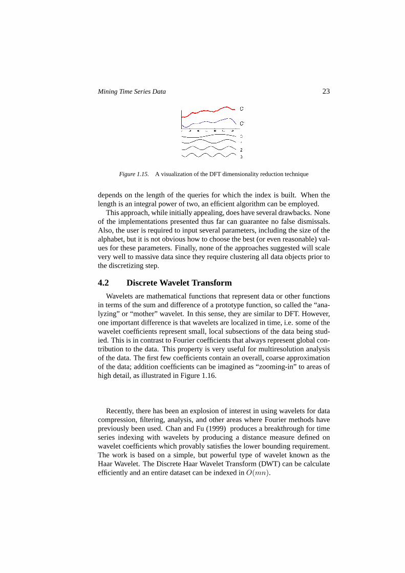
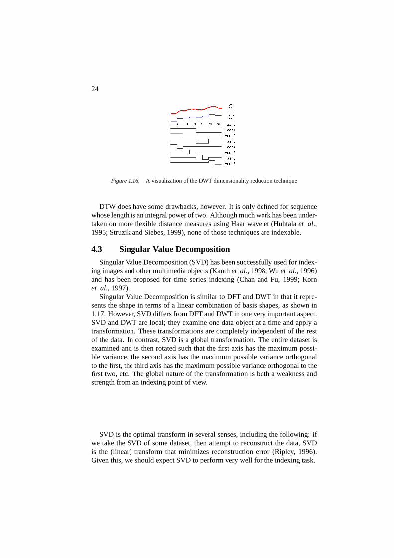
Wavelets are mathematical functions that represent data or other functionsin terms of the sum and difference of a prototype function, so called the “ana-lyzing” or “mother” wavelet. In this sense, they are similar to DFT. However,one important difference is that wavelets are localized in time, i.e. some of thewavelet coefficients represent small, local subsections of the data being stud-ied. This is in contrast to Fourier coefficients that always represent global con-tribution to the data. This property is very useful for multiresolution analysisof the data. The first few coefficients contain an overall, coarse approximationof the data; addition coefficients can be imagined as “zooming-in” to areas ofhigh detail, as illustrated in Figure 1.16.

Recently, there has been an explosion of interest in using wavelets for datacompression, filtering, analysis, and other areas where Fourier methods havepreviously been used. Chan and Fu (1999) produces a breakthrough for timeseries indexing with wavelets by producing a distance measure defined onwavelet coefficients which provably satisfies the lower bounding requirement.The work is based on a simple, but powerful type of wavelet known as theHaar Wavelet. The Discrete Haar Wavelet Transform (DWT) can be calculateefficiently and an entire dataset can be indexed inO(mn).

24

Figure 1.16. A visualization of the DWT dimensionality reduction technique

DTW does have some drawbacks, however. It is only defined for sequencewhose length is an integral power of two. Although much work has been under-taken on more flexible distance measures using Haar wavelet (Huhtalaet al.,1995; Struzik and Siebes, 1999), none of those techniques are indexable.

4.3 Singular Value Decomposition

Singular Value Decomposition (SVD) has been successfully used for index-ing images and other multimedia objects (Kanthet al., 1998; Wuet al., 1996)and has been proposed for time series indexing (Chan and Fu, 1999; Kornet al., 1997).

Singular Value Decomposition is similar to DFT and DWT in that it repre-sents the shape in terms of a linear combination of basis shapes, as shown in1.17. However, SVD differs from DFT and DWT in one very important aspect.SVD and DWT are local; they examine one data object at a time and apply atransformation. These transformations are completely independent of the restof the data. In contrast, SVD is a global transformation. The entire dataset isexamined and is then rotated such that the first axis has the maximum possi-ble variance, the second axis has the maximum possible variance orthogonalto the first, the third axis has the maximum possible variance orthogonal to thefirst two, etc. The global nature of the transformation is both a weakness andstrength from an indexing point of view.

SVD is the optimal transform in several senses, including the following: ifwe take the SVD of some dataset, then attempt to reconstruct the data, SVDis the (linear) transform that minimizes reconstruction error (Ripley, 1996).Given this, we should expect SVD to perform very well for the indexing task.


Figure 1.17. A visualization of the SVD dimensionality reduction technique.

4.4 Piecewise Linear Approximation

The idea of using piecewise linear segments to approximate time series datesback to 1970s (Pavlidis and Horowitz, 1974). This representation has numer-ous advantages, including data compression and noise filtering. There are nu-merous algorithms available for segmenting time series, many of which werepioneered by (Pavlidis and Horowitz, 1974). Figure 1.18 shows an example ofa time series represented by piecewise linear segments.

Figure 1.18. A visualization of the PLA dimensionality reduction technique

An open question is how to best chooseK, the “optimal” number of seg-ments used to represent a particular time series. This problem involves a trade-off between accuracy and compactness, and clearly has no general solution.

4.5 Piecewise Aggregate Approximation

The recent work (Keoghet al., 2001; Yi and Faloutsos, 2000) (indepen-dently) suggest approximating a time series by dividing it into equal-lengthsegments and recording the mean value of the data points that fall within the

26

segment. The authors use different names for this representation. For clar-ity here, we refer to it as Piecewise Aggregate Approximation (PAA). Thisrepresentation reduces the data fromn dimensions toN dimensions by divid-ing the time series intoN equi-sized ‘frames’. The mean value of the datafalling within a frame is calculated, and a vector of these values becomes thedata reduced representation. WhenN = n, the transformed representation isidentical to the original representation. WhenN = 1, the transformed rep-resentation is simply the mean of the original sequence. More generally, thetransformation produces a piecewise constant approximation of the originalsequence, hence the name, Piecewise Aggregate Approximation (PAA). Thisrepresentation is also capable of handling queries of variable lengths.

Figure 1.19. A visualization of the PAA dimensionality reduction technique

In order to facilitate comparison of PAA with other dimensionality reduc-tion techniques discussed earlier, it is useful to visualize it as approximatinga sequence with a linear combination of box function. Figure 1.19 illustratesthis idea.

This simple technique is surprisingly competitive with the more sophisti-cated transform. In addition, the fact that each segment in PAA is of the samelength facilitates indexing of this representation.

4.6 Adaptive Piecewise Constant Approximation

As an extension to the PAA representation, Adaptive Piecewise ConstantApproximation (APCA) is introduced (Keoghet al., 2001). This represen-tation allows the segments to have arbitrary lengths, which in turn needs twonumbers per segment. The first number records the mean value of all the datapoints in segment, and the second number records the length of the segment.

It is difficult to make any intuitive guess about the relative performance ofthe two techniques. On one had, PAA has the advantage of having twice as


many approximating segments. On the other hand, APCA has the advantageof being able to place a single segment in an area of low activity and manysegments in areas of high activity. In addition, one has to consider the structureof the data in question. It is possible to construct artificial datasets, where oneapproach has an arbitrarily large reconstruction error, while the other approachhas reconstruction error of zero.

Figure 1.20. A visualization of the APCA dimensionality reduction technique

In general, finding the optimal piecewise polynomial representation of atime series requires aO(Nn2) dynamic programming algorithm (Faloutsoset al., 1997). For most purposed, however, an optimal representation is not re-quired. Most researchers, therefore, use a greedy suboptimal approach instead(Keogh and Smyth, 1997). In (Keoghet al., 2001), the authors utilize an orig-inal algorithm which produces high quality approximations inO(nlog(n)).The algorithm works by first converting the problem into a wavelet compres-sion problem, for which there are well-known optimal solutions, then convert-ing the solution back to the APCA representation and (possible) making minormodification.

4.7 Symbolic Aggregate Approximation (SAX)

Symbolic Aggregate Approximation is a novel symbolic representation fortime series recently introduced by (Linet al., 2003), which has been shown topreserve meaningful information from the original data and produce competi-tive results for classifying and clustering time series.

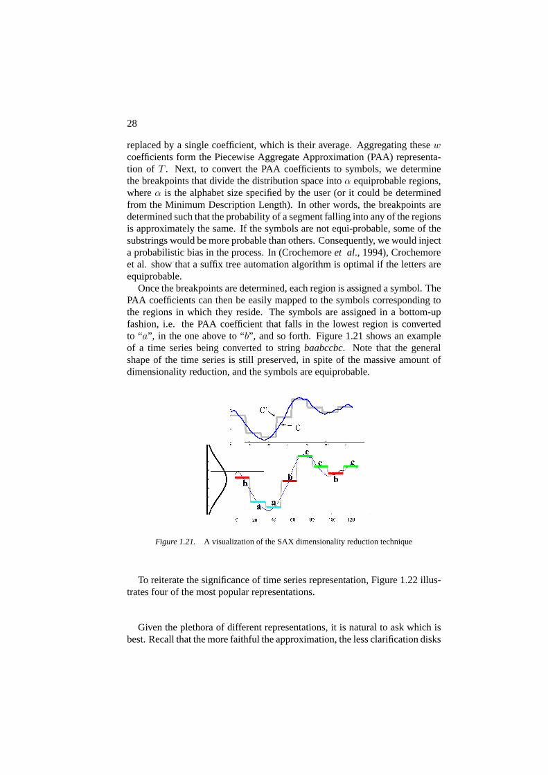
The basic idea of SAX is to convert the data into a discrete format, with asmall alphabet size. In this case, every part of the representation contributesabout the same amount of information about the shape of the time series. Toconvert a time series into symbols, it is first normalized, and two steps of dis-cretization will be performed. First, a time seriesT of lengthn is divided intow equal-sized segments; the values in each segment are then approximated and

28

replaced by a single coefficient, which is their average. Aggregating thesewcoefficients form the Piecewise Aggregate Approximation (PAA) representa-tion of T . Next, to convert the PAA coefficients to symbols, we determinethe breakpoints that divide the distribution space intoα equiprobable regions,whereα is the alphabet size specified by the user (or it could be determinedfrom the Minimum Description Length). In other words, the breakpoints aredetermined such that the probability of a segment falling into any of the regionsis approximately the same. If the symbols are not equi-probable, some of thesubstrings would be more probable than others. Consequently, we would injecta probabilistic bias in the process. In (Crochemoreet al., 1994), Crochemoreet al. show that a suffix tree automation algorithm is optimal if the letters areequiprobable.

Once the breakpoints are determined, each region is assigned a symbol. ThePAA coefficients can then be easily mapped to the symbols corresponding tothe regions in which they reside. The symbols are assigned in a bottom-upfashion, i.e. the PAA coefficient that falls in the lowest region is convertedto “a”, in the one above to “b”, and so forth. Figure 1.21 shows an exampleof a time series being converted to stringbaabccbc. Note that the generalshape of the time series is still preserved, in spite of the massive amount ofdimensionality reduction, and the symbols are equiprobable.

Figure 1.21. A visualization of the SAX dimensionality reduction technique

To reiterate the significance of time series representation, Figure 1.22 illus-trates four of the most popular representations.

Given the plethora of different representations, it is natural to ask which isbest. Recall that the more faithful the approximation, the less clarification disks


Figure 1.22. Four popular representations of time series. For each graphic, we see a raw timeseries of length 128. Below it, we see an approximation using 1/8 of the original space. In eachcase, the representation can be seen as a linear combination of basis functions. For example,the Discrete Fourier representation can be seen as a linear combination of the four sine/cosinewaves shown in the bottom of the graphics.

30

accesses we will need to make in Step 3 of Table 1.1. In the example shown inFigure 1.22, the discrete Fourier approach seems to model the original data thebest. However, it is easy to imagine other time series where another approachmight work better. There have been many attempts to answer the questionof which is the best representation, with proponents advocating their favoritetechnique (Chakrabartiet al., 2002; Faloutsoset al., 1994; Popivanovet al.,2002; Rafieiet al., 1998). The literature abounds with mutually contradic-tory statements such as “Several wavelets outperform the . . . DFT” (Popivanovet al., 2002), “DFT-base and DWT-based techniques yield comparable results”(Wu et al., 2000), “Haar wavelets perform . . . better than DFT” (Kahveciand Singh, 2001). However, an extensive empirical comparison on 50 diversedatasets suggests that while some datasets favor a particular approach, overall,there is little difference between the various approaches in terms of their abilityto approximate the data (Keogh and Kasetty, 2002). There are however, otherimportant differences in the usability of each approach (Chakrabartiet al.,2002). We will consider some representative examples of strengths and weak-nesses below.

The wavelet transform is often touted as an ideal representation for time se-ries data mining, because the first few wavelet coefficients contain informationabout the overall shape of the sequence while the higher order coefficients con-tain information about localized trends (Popivanovet al., 2002; Shahabiet al.,2000). This multiresolution property can be exploited by some algorithms, andcontrasts with the Fourier representation in which every coefficient representsa contribution to the global trend (Faloutsoset al., 1994; Rafieiet al., 1998).However, wavelets do have several drawbacks as a data mining representation.They are only defined for data whose length is an integer power of two. Incontrast, the Piecewise Constant Approximation suggested by (Yi and Falout-sos, 2000), has exactly the fidelity of resolution of as the Haar wavelet, but isdefined for arbitrary length time series. In addition, it has several other usefulproperties such as the ability to support several different distance measures (Yiand Faloutsos, 2000), and the ability to be calculated in an incremental fash-ion as the data arrives (Chakrabartiet al., 2002). One important feature of allthe above representation is that they are real values. This somewhat limits thealgorithms, data structures, and definitions available for them. For example, inanomaly detection, we cannot meaningfully define the probability of observingany particular set of wavelet coefficients, since the probability of observing anyreal number is zero. Such limitations have lead researchers to consider using asymbolic representation of time series (Linet al., 2003).


5. Summary

In this chapter, we have reviewed some major tasks in time series data min-ing. Since time series data are typically very large, discovering informationfrom these massive data becomes a challenge, which leads to the enormousresearch interests in approximating the data in reduced representation. Thedimensionality reduction of the data has now become the heart of time seriesdata mining and is the primary step to efficiently deal with data mining tasksfor massive data. We review some of important time series representationsproposed in the literature. We would like to emphasize that the key step in anysuccessful time series data mining endeavor always lies in choosing the rightrepresentation for the task at hand.

Notes1. In unusual situations, it might be more appropriate not to normalize the data, e.g. when offset and

amplitude changes are important.

References

Aach, J. and Church, G. Aligning gene expression time series with time warp-ing algorithms. Bioinformatics; 2001, Volume 17, pp. 495-508.

Aggarwal, C., Hinneburg, A., Keim, D. A. On the surprising behavior of dis-tance metrics in high dimensional space. In proceedings of the 8th Inter-national Conference on Database Theory; 2001 Jan 4-6; London, UK, pp420-434.

Agrawal, R., Faloutsos, C., Swami, A. Efficient Similarity Search in SequenceData bases. International Conference on Foundations of Data Organization(FODO); 1993.

Agrawal, R., Lin, K.-I., Sawhney, H.S., Shim, K. Fast Similarity Search in thePresence of Noise, Scaling, and Translation in Trime-Series Databases. Pro-ceedings of 21st International Conference on Very Large Databases (VLDB);1995 Sep; Zurich, Switzerland, pp. 490-500.

Berndt, D.J., Clifford, J. Finding Patterns in Time Series: A Dynamic Program-ming Approach. In Advances in Knowledge Discovery and Data MiningAAAI/MIT Press, Menlo Park, CA, 1996, pp. 229-248.

Bollobas, B., Das, G., Gunopulos, D., Mannila, H. Time-Series Similarity Prob-lems and Well-Separated Geometric Sets. Nordic Jour. of Computing 2001;4.

Brin, S. Near neighbor search in large metric spaces. Proceedings of 21st

VLDB; 1995.Chakrabarti, K., Keogh, E., Pazzani, M., Mehrotra, S. Locally adaptive dimen-

sionality reduction for indexing large time series databases. ACM Transac-tions on Database Systems. Volume 27, Issue 2, (June 2002). pp 188-228.

32

Chan, K., Fu, A.W. Efficient time series matching by wavelets. Proceedings of15th IEEE International Conference on Data Engineering; 1999 Mar 23-26;Sydney, Australia, pp. 126-133.

Chang, C.L.E., Garcia-Molina, H., Wiederhold, G. Clustering for Approxi-mate Similarity Search in High-Dimensional Spaces. IEEE Transactions onKnowledge and Data Engineering 2002; Jul – Aug, 14(4): 792-808.

Chiu, B.Y., Keogh, E., Lonardi, S. Probabilistic discovery of time series motifs.Proceedings of ACM SIGKDD; 2003, pp. 493-498.

Ciaccia, P., Patella, M., Zezula, P. M-tree: An efficient access method for sim-ilarity search in metric spaces. Proceedings of 23rd VLDB; 1997, pp. 426-435.

Crochemore, M., Czumaj, A., Gasjeniec, L, Jarominek, S., Lecroq, T.,Plandowski, W., Rytter, W. Speeding up two string-matching algorithms.Algorithmica; 1994; Vol. 12(4/5), pp. 247-267.

Dasgupta, D., Forrest, S. Novelty Detection in Time Series Data Using Ideasfrom Immunology. Proceedings of 8th International conference on Intelli-gent Systems; 1999 Jun 24-26; Denver, CO.

Debregeas, A., Hebrail, G. Interactive interpretation of kohonen maps appliedto curves. In proceedings of the 4th Int’l Conference of Knowledge Discov-ery and Data Mining; 1998 Aug 27-31; New York, NY, pp 179-183.

Faloutsos, C., Jagadish, H., Mendelzon, A., Milo, T. A signature techniquefor similarity-based queries. Proceedings of the International Conferenceon Compression and Complexity of Sequences; 1997 Jun 11-13; Positano-Salerno, Italy.

Faloutsos, C., Ranganathan, M., Manolopoulos, Y. Fast subsequence matchingin time-series databases. In proceedings of the ACM SIGMOD Int’l Con-ference on Management of Data; 1994 May 25-27; Minneapolis, MN, pp419-429.

Ge, X., Smyth, P. Deformable Markov Model Templates for Time-Series Pat-tern Matching. Proceedings of 6th ACM SIGKDD International Conferenceon Knowledge Discovery and Data Mining; 2000 Aug 20-23; Boston , MA,pp. 81-90.

Geurts, P. Pattern extraction for time series classification. Proceedings of Prin-ciples of Data Mining and Knowledge Discovery, 5th European Conference;2001 Sep 3-5; Freiburg, Germany, pp 115-127.

Goldin, D.Q., Kanellakis, P.C. On Similarity Queries for Time-Series Data:Constraint Specification and Implementation. Proceedings of the 1st Inter-national Conference on the Principles and Practice of Constraint Program-ming; 1995 Sep 19-22; Cassis, France, pp. 137-153.

Guralnik, V., Srivastava, J. Event detection from time series data. In proceed-ings of the 5th ACM SIGKDD Int’l Conference on Knowledge Discoveryand Data Mining; 1999 Aug 15-18; San Diego, CA, pp 33-42.


Huhtala, Y., Karkkainen, J, Toivonen, H. Mining for similarities in alignedtime series using wavelet. Data mining and Knowledge Discovery: Theory,Tools, and Technology, SPIE Proceedings Series 1995; Orlando, FL, Vol.3695, pp. 150-160.

Hochheiser, H., Shneiderman,, B. Interactive Exploration of Time-Sereis Data.Proceedings of 4th International conference on Discovery Science; 2001Nov 25-28; Washington, DC, pp. 441-446.

Indyk, P., Koudas, N., Muthukrishnan, S. Identifying representative trends inmassive time series data sets using sketches. In proceedings of the 26th Int’lConference on Very Large Data Bases; 2000 Sept 10-14; Cairo, Egypt, pp363-372.

Jagadish, H.V., Mendelzon, A.O., and Milo, T. Similarity-Based Queries. Pro-ceedings of ACM PODS; 1995 May; San Jose, CA, pp. 36-45.

Kahveci, T., Singh, A. Variable length queries for time series data. In pro-ceedings of the 17th Int’l Conference on Data Engineering; 2001 Apr 2-6;Heidelberg, Germany, pp 273-282.

Kalpakis, K., Gada, D., Puttagunta, V. Distance measures for effective clus-tering of ARIMA time-series. Proceedings of the IEEE Int’l Conference onData Mining; 2001 Nov 29-Dec 2; San Jose, CA, pp 273-280.

Kanth, K.V., Agrawal, D., Singh, A. Dimensionality reduction for similaritysearching in dynamic databases. Proceedings of ACM SIGMOD Interna-tional Conference; 1998, pp. 166-176.

Keogh, E. Exact indexing of dynamic time warping. Proceedings of 28th In-ternation Conference on Very Large Databases; 2002; Hong Kong, pp. 406-417.

Keogh, E., Chakrabarti, K., Mehrotra, S., Pazzani, M. Locally adaptive dimen-sionality reduction for indexing large time series databases. Proceedings ofACM SIGMOD International Conference; 2001.

Keogh, E., Chakrabarti, K., Pazzani, M., Mehrotra, S. Dimensionality reduc-tion for fast similarity search in large time series databases. Knowledge andInformation Systems 2001; 3: 263-286.

Keogh, E., Lin, J., Truppel, W. Clustering of Time Series Subsequences isMeaningless: Implications for Previous and Future Research. Proceedingsof ICDM; 2003, pp. 115-122.

Keogh, E., Lonardi, S., Chiu, W. Finding Surprising Patterns in a Time SeriesDatabase In Linear Time and Space. In the 8th ACM SIGKDD InternationalConference on Knowledge Discovery and Data Mining; 2002 Jul 23 – 26;Edmonton, Alberta, Canada, pp 550-556.

Keogh, E., Lonardi, S., Ratanamahatana, C.A. Towards Parameter-Free DataMining. Proceedings of 10th ACM SIGKDD International Conference onKnowledge Discovery and Data Mining; 2004 Aug 22-25; Seattle, WA.

34

Keogh, E., Pazzani, M. An enhanced representation of time series which allowsfast and accurate classification, clustering and relevance feedback. Proceed-ings of the 4th Int’l Conference on Knowledge Discovery and Data Mining;1998 Aug 27-31; New York, NY, pp 239-241.

Keogh, E. and Kasetty, S. On the Need for Time Series Data Mining Bench-marks: A Survey and Empirical Demonstration. In the 8th ACM SIGKDDInternational Conference on Knowledge Discovery and Data Mining; 2002Jul 23 – 26; Edmonton, Alberta, Canada, pp 102-111.

Keogh, E., Smyth, P. A Probabilistic Approach to Fast Pattern matching inTime Series Databases. Proceedings of 3rd International conference onKnowledge Discovery and Data Mining; 1997 Aug 14-17; Newport Beach,CA, pp. 24-30.

Korn, F., Jagadish, H., Faloutsos, C. Efficiently supporting ad hoc queries inlarge datasets of time sequences. Proceedings of SIGMOD InternationalConferences 1997; Tucson, AZ, pp. 289-300.

Kruskal, J.B., Sankoff, D., Editors. Time Warps, String Edits, and Macro-molecules: The Theory and Practice of Sequence Comparison. Addison-Wesley, 1983.

Lin, J., Keogh, E., Lonardi, S., Chiu, B. A Symbolic Representation of TimeSeries, with Implications for Streaming Algorithms. Workshop on ResearchIssues in Data Mining and Knowledge Discovery, 8th ACM SIGMOD; 2003Jun 13; San Diego, CA.

Lin, J., Keogh, E., Lonardi, S., Lankford, J. P., Nystrom, D. M. Visually Min-ing and Monitoring Massive Time Series. Proceedings of the 10th ACMSIGKDD International Conference on Knowledge Discovery and Data Min-ing; 2004 Aug 22-25; Seattle, WA.

Ma, J., Perkins, S. Online Novelty Detection on Temporal Sequences. Pro-ceedings of 9th International Conference on Knowledge Discovery and DataMining; 2003 Aug 24-27; Washington DC.

Nievergelt, H., Hinterberger, H., Sevcik, K.C. The grid file: An adaptable, sym-metricmultikey file structure. ACM Trans. Database Systems; 1984; 9(1):38-71.

Palpanas, T., Vlachose, M, Keogh, E., Gunopulos, D., Truppel, W. OnlineAmnestic Approximation of Streaming Time Series. Proceedings of 20th

International Conference on Data Engineering; 2004, Boston, MA.Pavlidis, T., Horowitz, S. Segmentation of plane curves. IEEE Transactions on

Computers; 1974 August; Vol. C-23(8), pp. 860-870.Popivanov, I., Miller, R. J. Similarity search over time series data using wavelets.

In proceedings of the 18th Int’l Conference on Data Engineering; 2002 Feb26-Mar 1; San Jose, CA, pp 212-221.


Rafiei, D., Mendelzon, A. O. Efficient retrieval of similar time sequences usingDFT. In proceedings of the 5th Int’l Conference on Foundations of DataOrganization and Algorithms; 1998 Nov 12-13; Kobe, Japan.

Ratanamahatana, C.A., Keogh, E. Making Time-Series Classification MoreAccurate Using Learned Constrints. Proceedings of SIAM International Con-ference on Data Mining; 2004 Apr 22-24; Lake Buena Vista, FL, pp.11-22.

Ripley, B.D. Pattern recognition and neural networks. Cambridge UniversityPress, Cambridge, UK, 1996.

Robinson, J.T. The K-d-b-tree: A search structure for large multidimensionaldynamic indexes. Proceedings of ACM SIGMOD; 1981.

Shahabi, C., Tian, X., Zhao, W. TSA-tree: a wavelet based approach to improvethe efficiency of multi-level surprise and trend queries. In proceedings of the12th Int’l Conference on Scientific and Statistical Database Management;2000 Jul 26-28; Berlin, Germany, pp 55-68.

Struzik, Z., Siebes, A. The Haar wavelet transform in the time series similarityparadigm. Proceedings of 3rd European Conference on Principles and Prac-tice of Knowledge Discovery in Databases; 1999; Prague, Czech Republic,pp. 12-22.

Tufte, E. The visual display of quantitative information. Graphics Press,Cheshire, Connecticut, 1983.

Tzouramanis, T., Vassilakopoulos, M., Manolopoulos, Y. Overlapping LinearQuadtrees: A Spatio-Temporal Access Method. ACM-GIS; 1998, pp. 1-7.

Guralnik, V., Srivastava, J. Event Detection from Time Series Data. Proceed-ings of ACM SIGKDD; 1999, pp 33-42.

Vlachos, M., Gunopulos, D., Das, G. Rotation Invariant Distance Measures forTrajectories. Proceedings of 10th International Conference on KnowledgeDiscovery and Data Mining; 2004 Aug 22-25; Seattle, WA.

Vlachos, M., Meek, C., Vagena, Z., Gunopulos, D. Identification of Similari-ties, Periodicities & Bursts for Online Search Queries. Proceedings of Inter-national Conference on Management of Data; 2004; Paris, France.

Weber, M., lexa, M., Muller, W. Visualizing Time Series on Spirals. Proceed-ings of IEEE Symposium on Information Visualization; 2000 Oct 21-26;San Diego, CA, pp. 7-14.

Wijk, J.J. van, E. van Selow. Cluster and calendar-based visualization of timeseries data. Proceedings of IEEE Symposium on Information Visualization;1999 Oct 25-26, IEEE Computer Society, pp 4-9.

Wu, D., Agrawal, D., El Abbadi, A., Singh, A, Smith, T.R. Efficient retrievalfor browsing large image databases. Proceedings of 5th International Con-ference on Knowledge Information; 1996; Rockville, MD, pp. 11-18.

Wu, Y., Agrawal, D., El Abbadi, A. A comparison of DFT and DWT basedsimilarity search in time-series databases. In proceedings of the 9th ACM

36

CIKM Int’l Conference on Information and Knowledge Management; 2000Nov 6-11; McLean, VA, pp 488-495.

Yi, B., Faloutsos, C. Fast time sequence indexing for arbitrary lp norms. Pro-ceedings of the 26th Int’l Conference on Very Large Databases; 2000 Sep10-14; Cairo, Egypt, pp 385-394.

Yianilos, P. Data structures and algorithms for nearest neighbor search in gen-eral metric spaces. Proceedings of 3rd SIAM on Discrete Algorithms; 1992.

Zhu, Y., Shasha, D. StatStream: Statistical Monitoring of Thousands of DataStreams in Real Time, Proceedings of VLDB; 2002, pp. 358-369.

chapter 1 mining time series datajessica/bookchaptertsmining.pdfchapter 1 mining time series data...

Documents