Takustr. 714195 Berlin

GermanyZuse Institute Berlin

ADRIAN SALI

Coupling of Monodomain and Eikonal Modelsfor Cardiac Electrophysiology

ZIB Report 16-50 (October 2016)

Zuse Institute BerlinTakustr. 7D-14195 Berlin

Telefon: +49 30-84185-0Telefax: +49 30-84185-125

e-mail: bibliothek@zib.deURL: http://www.zib.de

ZIB-Report (Print) ISSN 1438-0064ZIB-Report (Internet) ISSN 2192-7782

Coupling of Monodomain and EikonalModels for Cardiac Electrophysiology∗

Adrian Sali

October 4, 2016

∗Thesis submitted for the degree Master of Science in the Department of Mathematics andComputer Science, Free University Berlin. Advisor Dr. Martin Weiser.

Abstract

The primary goal of this paper is to study the coupling of monodomain and eikonalmodels for the numerical simulation of cardiac electrophysiology.

Eikonal models are nonlinear elliptic equations describing the excitation time of thecardiac tissue. They are often used as very fast approximations for monodomainor bidomain models - parabolic reaction-diffusion systems describing the excitationwavefront in terms of ionic currents. The excitation front is a thin region with highgradients, whereas excitation times vary over larger domains. Hence, eikonal equa-tions can be solved on much coarser grids than monodomain equations. Moreover,as eikonal models are not time-dependent, no time integration is needed.

Eikonal models are derived from monodomain models making additional assump-tions and using certain approximations. While generally the approximation is rathergood, several specific situations are not well captured by eikonal models. We considercoupling the two models, i.e. using the monodomain model in regions where moreaccurate results or the shape of the wavefront are needed, and the eikonal model inthe remaining parts of the domain, where the excitation time is sufficient. Restrict-ing the monodomain simulation to a small subdomain reduces the computationaleffort considerably.

Numerical methods for the simulation of the individual models are presented, withthe finite element method as the main ingredient. Coupling conditions as well asalgorithms for implementing the coupling are explained. The approximation qualityand efficiency of the coupled model is illustrated on simple geometries using anAliev-Panfilov membrane model.

i

Contents

1 Introduction 11.1 Functioning of the heart . . . . . . . . . . . . . . . . . . . . . . . . . 21.2 Computational Models . . . . . . . . . . . . . . . . . . . . . . . . . . 41.3 Structure of the thesis . . . . . . . . . . . . . . . . . . . . . . . . . . 5

2 Models of Myocardial Behaviour 72.1 The Monodomain Model . . . . . . . . . . . . . . . . . . . . . . . . . 7

2.1.1 Derivation of the model . . . . . . . . . . . . . . . . . . . . . 82.1.2 Ionic Models . . . . . . . . . . . . . . . . . . . . . . . . . . . 11

2.2 The Eikonal Model . . . . . . . . . . . . . . . . . . . . . . . . . . . . 13

3 Numerical Solution Methods 203.1 The Monodomain Model . . . . . . . . . . . . . . . . . . . . . . . . . 20

3.1.1 Time discretization . . . . . . . . . . . . . . . . . . . . . . . . 203.1.2 Space discretization . . . . . . . . . . . . . . . . . . . . . . . 223.1.3 The linear system . . . . . . . . . . . . . . . . . . . . . . . . 25

3.2 The Eikonal Model . . . . . . . . . . . . . . . . . . . . . . . . . . . . 253.2.1 Space discretization . . . . . . . . . . . . . . . . . . . . . . . 283.2.2 The nonlinear system . . . . . . . . . . . . . . . . . . . . . . 28

4 Model coupling 324.1 The need for coupling . . . . . . . . . . . . . . . . . . . . . . . . . . 324.2 Coupling Conditions . . . . . . . . . . . . . . . . . . . . . . . . . . . 334.3 Numerical implementation . . . . . . . . . . . . . . . . . . . . . . . . 34

5 Numerical Results 425.1 Independent simulations . . . . . . . . . . . . . . . . . . . . . . . . . 425.2 Coupling with one excitation source . . . . . . . . . . . . . . . . . . 455.3 Coupling with two excitation sources . . . . . . . . . . . . . . . . . . 505.4 Eikonal model with a scar . . . . . . . . . . . . . . . . . . . . . . . . 53

6 Conclusion 56

Bibliography 58

ii

List of Figures

1.1 Internal view of the heart [42]. . . . . . . . . . . . . . . . . . . . . . 21.2 Cardiac myocyte [29]. . . . . . . . . . . . . . . . . . . . . . . . . . . 3

2.1 Comparison of the terms inside the integrals in (2.58). . . . . . . . . 17

3.1 Basis function. Image adapted from [40]. . . . . . . . . . . . . . . . . 24

4.1 Example domain used to illustrate the coupling method. . . . . . . . 344.2 Wavefront curvature at an artificial boundary. . . . . . . . . . . . . . 354.3 Example domain with extended regions. . . . . . . . . . . . . . . . . 364.4 Comparison of the front approximation using (4.9) and the mon-

odomain simulation result. . . . . . . . . . . . . . . . . . . . . . . . . 384.5 Example domain with extended regions in the more general case. . . 40

5.1 Monodomain simulation results at t = 18 ms. . . . . . . . . . . . . . 435.2 Monodomain simulation results. . . . . . . . . . . . . . . . . . . . . . 445.3 Eikonal simulation results. . . . . . . . . . . . . . . . . . . . . . . . . 445.4 Wavefront position comparison for the monodomain and eikonal so-

lutions at 6 ms intervals (monodomain - green, eikonal - white). . . . 455.5 Coupling geometry. . . . . . . . . . . . . . . . . . . . . . . . . . . . . 465.6 Wavefront position comparison for the full monodomain and model

coupling solutions at 3 ms intervals (full monodomain - green, coupling- orange). . . . . . . . . . . . . . . . . . . . . . . . . . . . . . . . . . 47

5.7 Flux at the right common boundary for the monodomain and eikonalregions. . . . . . . . . . . . . . . . . . . . . . . . . . . . . . . . . . . 47

5.8 A more accurate solution of the coupling problem (full monodomain- green, coupling - orange). . . . . . . . . . . . . . . . . . . . . . . . 48

5.9 Flux at the right common boundary for the monodomain and eikonalregions for the more accurate solution. . . . . . . . . . . . . . . . . . 48

5.10 Difference between the full monodomain and coupling solutions onΩMR at t = 24 ms. . . . . . . . . . . . . . . . . . . . . . . . . . . . . 49

5.11 Domain extensions for the simulation with two sources. . . . . . . . 50

iii

5.12 Wavefront position comparison for the full monodomain and modelcoupling solutions for two sources, with isolines at 3 ms intervals (fullmonodomain - green, coupling - orange). . . . . . . . . . . . . . . . . 51

5.13 Coupling with two sources. Flux at the left common boundary forthe eikonal and monodomain regions. . . . . . . . . . . . . . . . . . . 52

5.14 Coupling with two sources. Flux at the right common boundary forthe eikonal and monodomain regions. . . . . . . . . . . . . . . . . . . 52

5.15 Coupling geometry in the presence of scarred tissue. . . . . . . . . . 535.16 Wavefront position comparison for the full monodomain, model cou-

pling and eikonal solutions in the presence of scarred tissue, withisolines at 3 ms intervals (full monodomain - green, coupling - orange,eikonal - black). . . . . . . . . . . . . . . . . . . . . . . . . . . . . . . 54

5.17 Coupling geometry in the presence of a very thin scarred tissue (fullmonodomain - green, coupling - orange, eikonal - white). . . . . . . . 54

1 Introduction

Cardiovascular diseases are the leading cause of mortality in the world. In 2012, they

led to 17.5 million deaths. This number is expected to increase to 22.2 million by 2030

[33]. In the USA alone, 610’000 people die yearly because of heart diseases, which

represents one in four deaths [47]. Thus, the development of improved diagnose

and treatment procedures thereof is of utmost importance. This, in turn, requires a

better understanding of the actual functioning of the heart.

Current experimental methods of studying the activity of the heart are often too

invasive. For example, an electrophysiology study involves the percutaneous intro-

duction of electrode catheters [52]. Unsuitable catheters may lead to punctures in

the wall tissue which could lead to internal bleedings [14]. The procedure might

also stimulate severe rhythm problems and may, rarely, cause the perforation of the

heart [11].

On the other hand, less invasive procedures do not provide the same level of detail.

For instance, in electrocardiograms, the solution of an inverse problem is necessary

in order to determine the actual activity of the heart. A mathematical model would

help determine important physiological parameters by applying realistic physical

constraints to the inverse problem [45].

Computational models would not pose risks to the patients. Moreover, they are not

subject to the ethics procedures that would be required for performing experiments

on either people or animals. Additionally, even when experimental studies are carried

out, they never provide measurements for all the functional elements of the heart.

Computer simulations would help both in simulating unavailable events and also in

understanding better the data acquired.

1

1.1 Functioning of the heart

Figure 1.1: Internal view of the heart [42].

1.1 Functioning of the heart

The main role of the heart is pumping blood through the organism. The heart is

divided into four chambers: the right atrium and ventricle, and the left atrium and

ventricle. Initially, blood enters the right atrium and flows into the right ventricle.

It then enters the pulmonary arteries that transport it to the lungs, where it is

oxygenated. Through the pulmonary veins it then returns to the left atrium and

then flows into the left ventricle. Finally, it is pumped to the body through the

aorta. Chambers and blood vessels are separated by valves, which, due to their

structure, ensure that the fluid flows in the correct direction.

The actual pumping is realized through the cyclic contraction and relaxation of a

muscle structure in the walls of the heart called myocardium, which is surrounded

by thin layers named endocardium - on the inside, and epicardium - on the outside.

The myocardium consists of discrete cells called myocytes that are bounded from

2

1.1 Functioning of the heart

Figure 1.2: Cardiac myocyte [29].

the extracellular space by a membrane - the sarcolemma. The myocytes are tube

shaped, with a length in between 50 and 120 µm and a diameter in the range between

5 and 25 µm [39]. The extracellular space contains water, electrolytes and collagen

fibers among others. For a more detailed discussion on the microscopic structure of

the heart, see [39, 44].

The excitation of the heart muscle is caused by an increase in the concentration of

intracellular Ca2+, due to its flow from the extracellular space to the interior of the

cell, through ion channels connecting the two media. Besides Ca2+, there are also

Na+, K+ and Cl− ionic currents across the lipid membrane of the cardiac cell. These

currents are generated by a wave of electrical activity that propagates through the

heart, called action potential. The wave is initiated by specialized myocytes in the

sino-atrial node situated at the top of the right atrium and is made possible by

the fact that the cardiac cells are excitable, and by the presence of gap junctions -

proteins that create channels between neighboring cells [43]. Note that due to the

tube-like shape of myocytes and their relatively parallel alignment, the myocardial

tissue is anisotropic and, consequently, the wave does not spread with the same

speed in different directions. The speed is higher along the cell and slower in the

other directions.

The rise in the concentration of Ca2+ is generated by a decrease in the (absolute

value of) transmembrane potential difference during depolarization (or upstroke),

the first stage of the action potential. Specifically, during depolarization, the poten-

tial difference increases from the resting value of about −80 mV to approximately

20 mV. The exact values depend on the area of the heart, age, species and other

3

1.2 Computational Models

physiological factors [5]. Thus, the study of this perturbation (depolarization wave-

front) is an important step in understanding the functioning of the myocardium. The

importance of this is further emphasized by the fact that anomalies in the electrical

propagation in the heart lead to or are caused by serious heart problems [43].

1.2 Computational Models

As the sinus node contains more than 100’000 cells, the atrium - several million

and the ventricle - hundreds of millions [35], modeling the spread of the electrical

excitation by simulating the ionic activity of each cardiac cell is not feasible. Cellular

automata have also been used as models of propagation [50], where each cell can be in

only a discrete number of states that change at discrete times. Its evolution depends

on its state at the previous time step and on its neighboring cells. This model is

computationally cheaper, but it has the disadvantage that it’s difficult to relate the

behavior of cellular automata to electrophysiological observations. Moreover, with a

regular lattice, the velocity-curvature relations of the wavefront cannot be simulated

readily [22]. Thus, macroscopic models that still observe the electrophysiological

aspects are required.

One such model is following the approach now generally known as the bidomain

model [20], and was initially proposed at the end of the 1970s [46, 23, 10]. The two

domains suggested by the model name are represented by the averaged properties

of the intracellular and extracellular media. The assumption on these domains is

that they are continuous, superposed, they interpenetrate and are connected by a

distributed cellular membrane. The current between them depends on the properties

of the cell membrane averaged over volume [45, 15]. Furthermore, assuming that the

anisotropy ratios of the domains are equal, a monodomain model can be derived.

In this thesis, the monodomain approach with an ionic model first introduced by

Aliev and Panfilov [1] is used. It is represented by a nonlinear reaction-diffusion

type system consisting of a parabolic PDE and an ODE. Its solution describes the

shape and position of the depolarization wavefront at each moment in time. Further

details are explained in Section 2.1. Due to its dependence on both space and time

4

1.3 Structure of the thesis

and, since a fine spatial discretization is needed at the wavefront for accurate results,

solving this system is still computationally expensive.

A less accurate eikonal model, requiring significantly fewer computing resources,

was derived by Keener [25] and Franzoni et al. [15] (see Section 2.2). In contrast

to the monodomain approach, the eikonal model does not simulate the shape of the

excitation front, but only its position. Specifically, it determines the excitation time

for each point in space. However, as it is represented by an elliptic PDE depending

only on space variables, no time integration is required for its numerical solution.

Moreover, unlike the transmembrane potential, the wave speed usually varies over

larger space scales. The gradients of the solution being smaller, a coarser grid can

be used for the numerical simulation.

Thus, from an application point of view, it would make sense to use the monodomain

model in the areas of the heart where a more accurate and detailed solution is needed,

and the eikonal model in the areas where a less accurate solution is sufficient. The

goal of this thesis is to present an approach for the coupling of these models.

1.3 Structure of the thesis

In Chapter 2 the monodomain and eikonal models are derived. The former is devel-

oped starting from physical laws, like conservation of current and Ohm’s Law. The

latter is derived from the monodomain model by making additional assumptions and

approximations.

Chapter 3 presents numerical solutions for both problems using the finite element

method. The linearly implicit Euler method is used for the time discretization of the

monodomain equations. The arising linear system is solved using the preconditioned

biconjugate gradient stabilized method. The nonlinear system resulting from the

discretization of the eikonal equation is solved by an error based damped Newton

algorithm.

Consequently, the need for coupling the two models is explained and the coupling

conditions and their numerical implementation are described in Chapter 4.

5

1.3 Structure of the thesis

Numerical results are included and discussed in Chapter 5. First, the results cor-

responding to the individual models are presented and compared. Then, results for

the coupling are shown for various geometries and use cases.

Finally, in Chapter 6 the methods and results are summarized and recommendations

for further work are suggested.

6

2 Models of Myocardial Behaviour

2.1 The Monodomain Model

The monodomain model is derived by making some additional assumptions on the

bidomain model. Therefore, we will first derive the former and then show its par-

ticular case - the monodomain model.

The bidomain model was first introduced by Tung [46] in 1978. It approximates the

intracellular and extracellular media as continuous spaces, that co-exist spatially

and that are separated by a cell membrane which is continuous as well and that

fills the entire volume. The spatial co-existence means that each point is part of

both media. The intracellular space can be considered continuous due to the gap

junctions between cells, which allow direct interaction between their internals. The

cell membrane has the role of insulating the two domains, which creates the potential

differences mentioned in the introductory chapter. Nonetheless, channels passing

through it allow ions to move from one medium to the other, thus creating a current

that depends on the potential difference between the two domains (transmembrane

potential) and on the permeability of the membrane. Due to continuity of the

domains, at each point we have a potential, that, from a physical point of view, is

the average over a small surrounding volume.

7

2.1 The Monodomain Model

2.1.1 Derivation of the model

Let Ji and Je be the intracellular and extracellular current densities respectively.

Assuming they each obey Ohm’s Law, we have

Ji = −Mi∇ui, (2.1)

Je = −Me∇ue, (2.2)

where ui and uj are the potentials of the domains, whereas Mi and Me are the

conductivities of the media. As heart tissue is anisotropic, these are tensor quantities.

Moreover, if we assume that capacitive, inductive, and electromagnetic propagative

effects can be neglected, conservation of current gives

∇ · Ji = −im, (2.3)

∇ · Je = im + iapp, (2.4)

where im is the outward transmembrane current per unit volume, and iapp is an

applied current per unit tissue volume.

Summing up (2.3) and (2.4) results in

∇ · Ji +∇ · Je = iapp, (2.5)

and plugging in (2.1) and (2.2) into (2.5), we obtain

∇ · (Mi∇ui) +∇ · (Me∇ue) = −iapp. (2.6)

Now let v := ui − ue be the transmembrane potential. The net current through the

membrane is equal to the sum of the ionic and capacitive components:

im = χIion + χCm∂v

∂t. (2.7)

Here, Cm is the capacitance of the membrane measured per unit area. The volt-

age/current relationship for capacitance I(t) = C ∂V (t)∂t has been used for the capac-

itive component. Additionally, a constant χ representing the area of cell membrane

per unit volume is introduced. The current Iion is also measured per unit area.

8

2.1 The Monodomain Model

Combining (2.1), (2.3) and (2.7), we obtain

∇ · (Mi∇ui) = χIion + χCm∂v

∂t, (2.8)

and using ui = v + ue in (2.8) and (2.6) we get the following system

∇ · (Mi∇(v + ue)) = χIion + χCm∂v

∂t, (2.9)

∇ · (Mi∇(v + ue)) +∇ · (Me∇ue) = −iapp. (2.10)

Finally, a rearrangement of terms results in the bidomain model

∇ · (Mi∇v) +∇ · (Mi∇ue) = χIion + χCm∂v

∂t, (2.11)

∇ · (Mi∇v) +∇ · ((Mi +Me)∇ue) = −iapp. (2.12)

For a full description of the model, boundary conditions are needed. In addition

to conservation of current between the intracellular and extracellular domain, this

condition should also be fulfilled between the heart muscle and the outside volume:

n · (Ji + Je) = n · Jo, (2.13)

where n is the boundary unit normal, while Jo is the current density corresponding

to the outside volume. Moreover, assuming that only the extracellular space is in

contact with the outside volume, it was shown [27] that the boundary condition

n · Ji = 0 (2.14)

should be satisfied. Using (2.1) and substituting ui by v + ue, this last relation is

equivalent to

n ·Mi∇(v + ue) = 0, (2.15)

whereas (2.13) becomes

n ·Me∇ue = n ·Mo∇uo, (2.16)

where uo is the potential of the outside volume, and Mo is the respective conductivity

tensor. We should also mention, that since the extracellular domain is in direct

9

2.1 The Monodomain Model

contact with the outer medium, the condition ue = uo should be satisfied.

In this thesis, we assume that the medium surrounding the heart is non-conductive.

Thus, in summary, the bidomain model can be formulated as follows:

∇ · (Mi∇v) +∇ · (Mi∇ue) = χIion + χCm∂v

∂ton Ω, (2.17)

∇ · (Mi∇v) +∇ · ((Mi +Me)∇ue) = −iapp on Ω, (2.18)

v(0,x) = v0(x) on Ω, (2.19)

ue(0,x) = ue0(x) on Ω, (2.20)

n ·Mi∇(v + ue) = 0 on ∂Ω, (2.21)

n ·Me∇ue = 0 on ∂Ω. (2.22)

For the derivation of the monodomain model, the assumption of equal anisotropy

ratios is made, i.e. Me = λMi, for some constant scalar λ. Substituting this into

(2.18) gives

∇ · (Mi∇v) + (1 + λ)∇ · (Mi∇ue) = −iapp, (2.23)

equivalent to

∇ · (Mi∇ue) = − 1

1 + λiapp −

1

1 + λ∇ · (Mi∇v). (2.24)

Replacing this in (2.17), we obtain

λ

1 + λ∇ · (Mi∇v)− 1

1 + λiapp = χIion + χCm

∂v

∂t. (2.25)

Equation (2.22) becomes

n · (λMi∇ue) = 0, (2.26)

and inserting this into (2.21), we get

n · (Mi∇v) = 0. (2.27)

Now, for vr - the resting potential, let

1

Rm:=

dIiondv

(vr) and1

rm:= χ

1

Rm, (2.28)

10

2.1 The Monodomain Model

and rm be the space average of rm. Further, define

τm := rmχCm, Mm := rmλ

1 + λMi, and fion := rmχIion. (2.29)

Again, rearranging and summarizing, we have the following monodomain model:

τm∂v

∂t= ∇ · (Mm∇v)− rm

1

1 + λiapp − fion on Ω (2.30)

n · (Mm∇v) = 0 on ∂Ω. (2.31)

Nondimensionalizing quantities, we obtain the form:

∂V

∂τ= ∇ · (M∇V ) + Iapp − Fion on Ω (2.32)

n · (M∇V ) = 0 on ∂Ω. (2.33)

2.1.2 Ionic Models

Finally, in order to solve these equations, a model for the ionic current Iion (Fion

respectively) is necessary. Currently, three main groups of ionic models are used

[43].

The models in the first one, called first generation, depict the ionic currents that

have the biggest role for the action potential, and describe both the cellular behav-

ior and the underlying physiology. Such models, however, do not describe fine-scale

physiological details. Hodgkin and Huxley first proposed a model of this kind [21].

It included a sodium, a potassium and a third current called leakage current. The

main disadvantage of this model in our case, however, is that it describes the action

potential in a squid giant axon, and is, therefore, not directly applicable to myocar-

dial cells. Later, in 1962, Noble [34] adapted it to work with the Purkinje fibre cells,

a tree-like structure located in the subendocardium. The leakage current is assumed

to be zero in this case, and the potassium current is separated into two distinct ones.

However, detailed physiological data had not yet been determined experimentally at

that time. Thus, the physiology behind the model was not accurate. It was enhanced

by improving the accuracy of the previously used ionic channels and by adding new

11

2.1 The Monodomain Model

ones in 1975 [32]. A model specific to ventricular cells was first introduced by Beeler

and Reuter [3] around the same time. Here, two outward potassium, one inward

calcium and one inward sodium currents are considered. Thus, it also depicts the

intracellular concentration of calcium, which has the main role in muscle contraction.

One final first generation model that we will mention here is due to Luo and Rudy

[31]. In addition to the Beeler-Reuter model, it decribes an additional potassium

current and a linear background current, comparable to the leakage current used by

Hodgkin and Huxley. Both these models are still widely used today.

Luo and Rudy significantly improved their model in 1994 [30]. Describing twelve

currents - including intracellular sodium, potassium and three distinct calcium con-

centrations - and several internal fluxes, this concept is part of the next group, called

second generation models. Other models that handle calcium ions differently have

been introduced in 1998 by Noble er al. [36] and by Jafri et al. [24]. In 1999,

Winslow et al. [51] proposed a similar model adapted to data from dogs. It includes

more than 30 state variables that control 13 ionic currents. It was later improved to

a model that contains several thousand variables by Greenstein and Winslow [19],

and was simplified by Greenstein et al. in 2006 [18]. Approaches using fractional

differential equations have also been suggested recently [49].

In the third group, phenomenological models are included. They simulate the ionic

current macroscopically, not at a cellular level. These are usually FitzHugh-Nagumo

[13] type models, with two variables. The first one is the transmembrane potential,

whereas the second one represents a gating variable. Thus, they are computationally

much cheaper, but they still reproduce the main characteristics of cardiac tissue.

Modifications of the simplified FitzHugh-Nagumo equations have been introduced

in 1991 by Kogan et al. [26], and by Rogers and McCulloch in 1994 [37]. The

latter has been further improved by Aliev and Panfilov in 1996 [1] by introducing

a nonlinearity in the description of the gating variable. Further, a model with two

gating variables was proposed by Fenton and Karma in 1998 [12].

Since our main goal is to study the propagation of the depolarization wavefront,

which is affected primarily by macroscopic properties, a model pertaining to the third

category described is used in this thesis, specifically, the Aliev-Panfilov approach.

12

2.2 The Eikonal Model

In this case, the monodomain model becomes:

∂V

∂τ= ∇ · (M∇V )−gaV (V − a)(V − 1)− V w + Iapp︸ ︷︷ ︸

:=f(V,w)

in Ω× (0, T ), (2.34)

∂w

∂τ=

(ε1 + µ1

w

V + µ2

)(−w − gsV (V − b− 1))︸ ︷︷ ︸

:=g(V,w)

in Ω× (0, T ), (2.35)

V (0,x) = V0(x) in Ω, (2.36)

w(0,x) = w0(x) in Ω, (2.37)

n · (M∇V ) = 0 on ∂Ω× (0, T ), (2.38)

n · (M∇w) = 0 on ∂Ω× (0, T ). (2.39)

Here all the terms are non-dimensional, the derivatives included. V is a representa-

tion of the potential difference across the membrane and varies between 0 (polarized

state) and 1 (depolarized state), w is a gating variable that corresponds to the con-

duction of a repolarising current, Iapp is the applied current and a is a threshold

parameter. The capacitance is included implicitly. Parameters ga, ε1, µ1, µ2, gs,

and b have no physiological meaning. Assuming a resting potential value of −80 mV

and an action potential amplitude of 100 mV, the real physical value of the trans-

membrane potential can be determined using

E [mV ] = 100V − 80. (2.40)

Existence of solutions for the weak formulation of a similar model, where the first

factor in g(V,w) is assumed to be a constant, was shown in [4].

2.2 The Eikonal Model

In many cases only the motion of the depolarization wavefront is of interest, and

not its shape. Under the assumption that the depolarization process starts only

in tissue at rest, a simplified model, called the eikonal model, can be derived. For

each point x in space, it determines its excitation time u(x), i.e. the time when the

transmembrane potential at the respective point is at the middle value between the

13

2.2 The Eikonal Model

resting and plateau potentials. The model was derived using singular perturbation

techniques by Franzoni, Guerri, and Rovida [15]. In this chapter, we will, however,

summarize the approach used by Tomlinson [45].

According to the definition of u(x) above, we have

v(x, u(x)) =1

2(vr + vp), (2.41)

where vr and vp are the resting and plateau transmembrane potentials.

In a healthy heart, the shape of the upstroke does not change significantly along the

tissue. Therefore, we may write

v(x, t) = vm(ω), (2.42)

where vm : R→ R is some function of variable ω, which is defined such that

v(x, u(x)) = vm(ω = 0). (2.43)

The change in coordinates

x = ξ and t = T (ξ, ω), (2.44)

therefore implies that

u(x) = T (ξ, 0). (2.45)

Define S(ξ, ω) by

S :=

(∂T

∂ω

)−1

. (2.46)

The chain rule gives

∂

∂ω=

d∑j=1

∂xj∂ω

∂

∂xj+∂t

∂ω

∂

∂t=∂T

∂ω

∂

∂t,

or∂

∂t= S

∂

∂ω. (2.47)

14

2.2 The Eikonal Model

Similarly,

∂

∂ξi=

d∑j=1

∂xj∂ξi

∂

∂xj+∂t

∂ξi

∂

∂t=

∂

∂xi+∂T

∂ξi

∂

∂t=

∂

∂xi+∂T

∂ξiS∂

∂ω,

or∂

∂xi=

∂

∂ξi− ∂T

∂ξiS∂

∂ω. (2.48)

Let us rewrite (2.30) in the original coordinates and using partial derivatives, as-

suming no external current is applied. We obtain

τm∂v

∂t=

d∑i=1

∂

∂xi

d∑j=1

µij∂v

∂xj

− fion, (2.49)

where µij are the elements of tensor Mm. Remembering that vm is only a function

of ω in the coordinates, we have

∂v

∂xj=

(∂

∂ξj− ∂T

∂ξjS∂

∂ω

)vm = − ∂T

∂ξjS∂vm∂ω

. (2.50)

Further, as Mm is independent of ω, we obtain

∂

∂xi

(µij

∂v

∂xj

)=

(∂

∂ξi− ∂T

∂ξiS∂

∂ω

)(−µij

∂T

∂ξjS∂vm∂ω

)= − ∂

∂ξi

(µijS

∂T

∂ξi

)∂vm∂ω

+∂T

∂ξiSµij

∂

∂ω

(S∂T

∂ξj

∂vm∂ω

)= − ∂

∂ξi

(µijS

∂T

∂ξi

)∂vm∂ω

+∂T

∂ξiSµij

(∂

∂ω

(S∂T

∂xj

)∂vm∂ω

+ S∂T

∂xj

∂2vm∂ω2

)= − ∂

∂ξi

(µijS

∂T

∂ξi

)∂vm∂ω

+ S∂T

∂ξi

∂

∂ω

(µijS

∂T

∂ξj

)∂vm∂ω

+ S2 ∂T

∂ξiµij

∂T

∂ξj

∂2vm∂ω2

(2.51)

15

2.2 The Eikonal Model

Thus, using the Einstein notation for summation, equation (2.30) becomes:(τmS +

∂

∂ξi

(Sµij

∂T

∂ξj

)− 1

2

∂

∂ω

(S2 ∂T

∂ξiµij

∂T

∂ξj

))dvmdω

= S2 ∂T

∂ξiµij

∂T

∂ξj

d2vmdω2

− fion.

(2.52)

We will now be looking for a first order approximation

T (ξ, ω) := T (ξ, 0) +ω

S(ξ, 0)= u(ξ) +

ω

s(ξ), (2.53)

that fits (2.52) as well as possible, where s(ξ) := S(ξ, 0). Therefore, we want to

minimize the residual

fion +

(τms+

∂

∂ξi

(sµij

∂T

∂ξj

)− 1

2

∂

∂ω

(s2 ∂T

∂ξiµij

∂T

∂ξj

))dvmdω− s2 ∂T

∂ξiµij

∂T

∂ξj

d2vmdω2

.

(2.54)

Simplifying, (2.54) becomes

fion +

(τms+ s

∂

∂ξi

(µij

∂T

∂ξj

))dvmdω− ∂

∂ω

(s2 ∂T

∂ξiµij

∂T

∂ξj

dvmdω

)(2.55)

To minimize this residual for all ω, two (since two parameters – u and s – need

to be determined) weighted integrals are set to zero. As we move away from the

wavefront, the propagation is less and less affected by the features at that point.

Therefore, Gaussians are selected as weights, specifically:

w1 = e−αω2

and w2 = ωe−αω2. (2.56)

Thus, we need

∞∫−∞

fionw1dω+

∞∫−∞

(τms+ s

∂

∂ξi

(µij

∂T

∂ξj

))dv

dωw1dω =

∞∫−∞

∂

∂ω

(s2 ∂T

∂ξiµij

∂T

∂ξj

dv

dω

)w1dω.

(2.57)

16

2.2 The Eikonal Model

Figure 2.1: Comparison of the terms inside the integrals in (2.58).

Applying Green’s theorem, and using (2.53) and (2.56), this becomes:

∞∫−∞

fione−αω2

dω +

(τms+ s

∂

∂ξi

(µij

∂u

∂ξj

)) ∞∫−∞

dvmdω

e−αω2dω

+ s∂

∂ξi

(µij

∂

∂ξj

(1

s

)) ∞∫−∞

dvmdω

ωe−αω2dω

= 2αs2 ∂u

∂ξjµij

∂u

∂ξj

∞∫−∞

dvmdω

ωe−αω2dω

+ 4αs2 ∂

∂ξi

(1

s

)µij

∂u

∂ξj

∞∫−∞

dvmdω

ω2e−αω2dω

+ 2αs2 ∂

∂ξi

(1

s

)µij

∂

∂ξj

(1

s

) ∞∫−∞

dvmdω

ω3e−αω2dω. (2.58)

Here, all integrals are constant. Further, it can be shown by dimensional analysis

(see [45] for details) that, by picking the scale of ω such that most of the variation

in v occurs over a unit change in ω, all terms on the right of the equation are small

compared to the second term on the left hand side. The same holds for the last term

on the left. The motivation for that can be seen in Fig. 2.1, where the derivative

of the expected front shape is plotted together with e−αω2, ωe−αω

2, and ω2e−αω

2

17

2.2 The Eikonal Model

for α = 0.5. One notices that the addition of ω in the products results in the

fact that the respective terms are small in the interval where the derivative of the

potential is large and vice-versa. Removing the insignificant terms, only the first

two components of the equation are left and we have the following approximation:

τms+ s∂

∂ξi

(µij

∂u

∂ξj

)≈ c2, (2.59)

for some constant c2.

Using the second weight parameter in (2.56), a similar reasoning leads to the second

equation for u and s:

s2 ∂u

∂ξiµij

∂u

∂ξj≈ c2

1. (2.60)

Using the same coordinate transformation in (2.31), we get that

∂T

∂ξiµijnj = 0, (2.61)

which at ω = 0 becomes

∂u

∂ξiµijnj = 0 on ∂Ω. (2.62)

Returning to the original coordinate system and summarizing (2.59), (2.60), and

(2.62), we obtain the system:

s

öu

∂xiµij

∂u

∂xj= c1 on Ω, (2.63)

τms+ s∂

∂xi

(µij

∂u

∂xj

)= c2 on Ω, (2.64)

∂u

∂xiµijnj = 0 on ∂Ω. (2.65)

Eliminating the variable s from this system finally gives the eikonal model

c0

√∇u ·Mm∇u−∇ · (Mm∇u) = τm on Ω, (2.66)

n ·M∇u+ αu = β on ∂Ω, (2.67)

18

2.2 The Eikonal Model

Symbol Name Unit SI unit

J Current density A ·m−2 A ·m−2

u, v Potential V V

M Conductivity Ω−1 ·m−1 kg−1 ·m−3 · s3 ·A2

i Current (per unit volume) A ·m−3 A ·m−3

Iion Ionic current (per unit area) A ·m−2 A ·m−2

C Capacitance (per unit area) F ·m−2 s4 ·A2 ·m−4 · kg−1

χ - m−1 m−1

Mm Coupling tensor m2 m2

τm Membrane time constant s s

Table 2.1: Units of the important parameters and variables.

where c0 := c2c1

. As we assumed no external current applied, to ”initiate” the front,

Dirichlet boundary conditions have to be assigned on some regions of the boundary.

Therefore, the boundary conditions have been generalized to Robin type.

To conclude the chapter, Table 2.1 contains a summary of the most important pa-

rameters and variables used in the model with their corresponding units physical.

19

3 Numerical Solution Methods

The monodomain and eikonal systems can only be solved analytically for a small

set of particular cases. For example, the exact solution of the eikonal model can

be determined in the case of an infinite homogeneous domain, where it describes an

ellipsoidal wavefront. For physically relevant domains, however, analytic solutions

cannot be determined. Therefore, numerical methods are employed to obtain ap-

proximate solutions. In this chapter we will present such methods for 2D domains.

The main ingredient here is the finite element method (FEM). For an in depth

discussion of the foundations of this method, see, for example, [2].

3.1 The Monodomain Model

The monodomain model is represented by a time- and space-dependent system of

equations. A discretization in both dimensions is therefore needed. The time inte-

gration is done using the linearly implicit Euler method, whereas space discretization

is implemented using the finite element method.

3.1.1 Time discretization

The monodomain model (2.34) - (2.39) is of the form

y = F (y), (3.1)

where

y =

(V

w

), (3.2)

20

3.1 The Monodomain Model

and F is a functional representing the right hand side.

The time domain [0, T ] is divided into subintervals 0 = t0 < · · · < tf < T . Then,

the system is solved using the linearly implicit Euler method. Specifically, we have

the discretization

yk+1 − yktk+1 − tk

= F (yk+1). (3.3)

Next, we linearize the right hand side to obtain

δykδtk

= F (yk) + (Fy(yk))δyk, (3.4)

where we denoted δyk := yk+1−yk and δtk := tk+1− tk. A rearrangement then gives

(I − δtkFy(yk))δyk = δtkF (yk), (3.5)

where I is the identity operator.

The solution at the new time step can then obviously be determined using

yk+1 = yk + δyk. (3.6)

The order of accuracy of the scheme could be improved by combining this approach

with τ -extrapolation, resulting in the so called extrapolated linearly implicit Euler

method [6]. For implementation details see [8].

Applying (3.5) to the monodomain equations gives

−δtk (∇ ·M∇δVk) + (1− δtkfV (Vk, wk))δVk

−δtkfw(Vk, wk)δwk = δtk∇ ·M∇Vk + δtkf(Vk, wk),

(3.7)

−δtkgV (Vk, wk)δVk + (1− δtkgw(Vk, wk))δwk = δtkg(Vk, wk), (3.8)

21

3.1 The Monodomain Model

where

fV (Vk, wk) = − ga ((2Vk − a)(Vk − 1) + Vk(Vk − a))− wk, (3.9)

fw(Vk, wk) = − Vk, (3.10)

gV (Vk, wk) = µ1wk

(Vk + µ2)2(−wk − gsVk(Vk − b− 1))

+

(ε1 + µ1

wkV + µ2

)(−gs(2Vk + b+ 1)),

(3.11)

gw(Vk, wk) =µ1

Vk + µ2(−wk − gsVk(Vk − b− 1))−

(ε1 + µ1

wkVk + µ2

). (3.12)

3.1.2 Space discretization

Notice the presence in (3.7) of the elliptic operator ∇·M∇ acting on δVk. Therefore,

at each time step we need to solve a stationary linear elliptic problem. To do that,

we rewrite the system in its weak form, by multiplying each equation with a test

function, integrating over the space domain and applying Green’s first identity. We

obtain:

δtk

∫Ω

∇δVk ·M∇φdx− δtk∫∂Ω

n ·M∇δVkφdx+

∫Ω

(1− δtkfV (Vk, wk))δVkφdx

−δtk∫Ω

fw(Vk, wk)δwkφdx = δtk

∫Ω

(∇ ·M∇Vk + f(Vk, wk))φdx

∀φ ∈ H1(Ω),

(3.13)

−δtk∫Ω

gV (Vk, wk)δVkψdx+

∫Ω

(1− δtkgw(Vk, wk))δwkψdx = δtk

∫Ω

g(Vk, wk)ψdx

∀ψ ∈ L2(Ω).

(3.14)

Note that the model we are using assumes homogeneous Neumann boundary condi-

tions, so, in theory the integral over the boundary of the domain should vanish in

equation (3.13). However, due to reasons displayed in Sec. 4.3, this assumption does

not hold on all the boundaries when coupling the model. Therefore, we generalize

22

3.1 The Monodomain Model

the boundary conditions to Robin type, i.e.

n ·M∇δVk + αδVk = β on δΩ. (3.15)

Plugging this into equation (3.13), it becomes

δtk

∫Ω

∇δVk ·M∇φdx+ δtk

∫∂Ω

αδVkφdx+

∫Ω

(1− δtkfV (Vk, wk))δVkφdx

−δtk∫Ω

fw(Vk, wk)δwkφdx = δtk

∫∂Ω

βφdx+ δtk

∫Ω

(∇ ·M∇Vk + f(Vk, wk))φdx

∀φ ∈ H1(Ω),

(3.16)

In the regions of the boundary where we have a homogeneous Neumann boundary

condition, α and β are set to 0. On the Dirichlet boundary, however, we pick a very

large α (≈ 108), and let β := αδVk0 , to introduce a penalty for the Neumann part of

the equation. Here, δVk0 represents the known value of the solution on the Dirichlet

boundary.

Solving this problem in the infinitely dimensional space H1(Ω)× L2(Ω) is not pos-

sible. Therefore, we want to find an approximation of the solution by solving it in a

finite dimensional subspace. We discretize this problem using linear finite elements.

First, we assume that the domain Ω has polygonal boundaries. Next, let T be a

triangulation of Ω, with N denoting the set of its nodes. A set T of triangles T is a

triangulation of Ω if

(i) Ω =⋃T∈T

T ,

(ii) The intersection of two triangles from T is either a common edge, a common

node, or empty.

Define the finite element space

S := y ∈ C0(Ω) | y is a linear polynomial on every T ∈ T , (3.17)

23

3.1 The Monodomain Model

Figure 3.1: Basis function. Image adapted from [40].

It satisfies

S × S ⊂ H1(Ω)× L2(Ω). (3.18)

To find solutions in S × S, we need to choose a basis of this space. For p ∈ N , let

λp ∈ S be a piecewise linear function satisfying

λp(q) = δpq ∀q ∈ N (Kronecker-δ). (3.19)

Then,

Λ := λp | p ∈ N (3.20)

is a basis of S called nodal basis.

Thus, we can represent δVk and δwk as linear combinations of these first order basis

functions:

δVk =∑p∈N

apλp and δwk =∑q∈N

aqλq. (3.21)

Plugging in this into (3.13) - (3.14), and choosing the basis functions as test func-

24

3.2 The Eikonal Model

tions, we obtain the following system for the unknowns ap, bq, ∀p, q ∈ N :

δtk∑p∈N

ap

∫Ω

∇λp ·M∇λrdx+ δtk∑p∈N

ap

∫∂Ω

αλpλrdx

+∑p∈N

ap

∫Ω

(1− δtkfV (Vk, wk))λpλrdx

−δtk∑q∈N

bq

∫Ω

fw(Vk, wk)λqλrdx = δtk

∫∂Ω

βλrdx

+δtk

∫Ω

(∇ ·M∇Vk + f(Vk, wk))λrdx

∀r ∈ N ,

(3.22)

−δtk∑p∈N

ap

∫Ω

gV (Vk, wk)λpλsdx+∑q∈N

bq

∫Ω

(1− δtkgw(Vk, wk))λqλsdx

= δtk

∫Ω

g(Vk, wk)λsdx ∀s ∈ N .(3.23)

3.1.3 The linear system

The integrals in (3.22) - (3.23) contain no unknown functions, and are, therefore,

constants that can be computed, for example, by a quadrature rule. Thus, we get a

sparse linear system, with 2|N | unknowns, where |N | is the cardinality of N .

To solve the resulting linear system, the preconditioned biconjugate gradient sta-

bilized method (Bi-CGSTAB) [48] is used - an iterative method that represents a

variant of the Bi-Conjugate Gradients approach. The algorithm is presented in Alg.

1, where K = K1K2 ≈ A is used as preconditioner. In our implementation, the

incomplete LU factorization [38] with fill level 1 is taken as preconditioner.

3.2 The Eikonal Model

The eikonal model does not depend on time. Therefore, only space discretization is

needed, and, again, the solution is determined using the finite element method. How-

25

3.2 The Eikonal Model

Algorithm 1 Preconditioned Bi-CGSTAB Algorithm [48]

let x0 be an initial guess;r0 = b−Ax0;let r0 be an arbitrary vector, such that (r0, r0) 6= 0, e.g. r0 = r0;ρ0 = α = ω0 = 1;v0 = p0 = 0;for i = 1, 2, 3, ... doρi = (r0, ri−1);β = (ρi/ρi−1)(α/ωi−1);pi = ri−1 + β(pi−1 − ωi−1vi−1);determine y from Ky = pi;vi = Ay;α = ρi/(r0, vi);s = ri−1 − αvi;determine z from Kz = s;t = Az;ωi = (K−1

1 t,K−11 s)/(K−1

1 t,K−11 t);

xi = xi−1 + αy + ωiz;if xi is accurate enough then

stop;end ifri = s− ωit;

end for

26

3.2 The Eikonal Model

ever, since the resulting elliptic problem is nonlinear, a nonlinear solver is required.

A damped Newton method has been chosen in this thesis.

Let us rewrite the eikonal model:

c0

√∇u ·M∇u−∇ · (M∇u) = τm on Ω, (3.24)

n ·M∇u+ αu = β on ∂Ω. (3.25)

As we are looking for a weak solution, we need to write equation (3.24) in its weak

formulation:

c0

∫Ω

√∇u ·M∇uφdx+

∫Ω

∇u ·M∇φdx−∫∂Ω

n ·M∇uφds =

∫Ω

τmφdx

∀φ ∈ H1(Ω). (3.26)

Using (3.25) and rearranging, we get:

c0

∫Ω

√∇u ·M∇uφdx+

∫Ω

∇u ·M∇φdx+

∫∂Ω

αuφds =

∫Ω

τmφdx+

∫∂Ω

βφds

∀φ ∈ H1(Ω). (3.27)

Additionally, ∂Ω can be divided into a Dirichlet boundary ΓD and a Neumann

boundary ΓN :

∂Ω = ΓD ∪ ΓN . (3.28)

As before, since on the Neumann boundary we have a homogeneous condition, α

and β must vanish there. On the Dirichlet boundary, however, we pick a very large

α (≈ 108), and let β := αu0, to introduce a penalty for the Neumann part of

equation (3.25). Here, u0 represents the known value of the solution on the Dirichlet

boundary. Using this and the fact that the boundary integrals in (3.27) can be

27

3.2 The Eikonal Model

written as the sum of the integrals over the two subdomains, we obtain:

c0

∫Ω

√∇u ·M∇uφdx+

∫Ω

∇u ·M∇φdx+

∫ΓD

αuφds =

∫Ω

τmφdx+

∫ΓD

βφds

∀φ ∈ H1(Ω). (3.29)

3.2.1 Space discretization

As for the monodomain model, we pick a conformal triangulation T E of the spatial

domain Ω, and let NE be its set of nodes. Analogously to (3.17), we define the

corresponding finite element space SE ⊂ H1(Ω), and basis functions λEp as in (3.19).

We can, therefore, decompose u as a linear combination of the basis functions:

u =∑p∈NE

cpλEp . (3.30)

Again, choosing the basis functions as test functions, equation (3.29) becomes:

c0

∫Ω

√√√√√∇ ∑p∈NE

cpλEp

·M∇ ∑p∈NE

cpλEp

λEq dx+∑p∈NE

cp

∫Ω

∇λEp ·M∇λEq dx+∑p∈NE

cp

∫ΓD

αλEp λEq ds =

∫Ω

τmλEq dx+

∫ΓD

βλEq ds

∀q ∈ NE . (3.31)

For the simulations in this thesis, second order basis functions have been used for

the eikonal model.

3.2.2 The nonlinear system

Notice that due to the presence of the square root in the first integral on the left

hand side, the system (3.31) is nonlinear. Therefore, a nonlinear solver is required.

28

3.2 The Eikonal Model

Let us write the general form of such a system:

find y such that F (y) = 0 (3.32)

The common method of solving such systems is (a modification of) Newton’s method.

Here, an initially chosen initial guess of the solution is iteratively improved on. In

the simplest variant of Newton’s method, the iteration is

Fy(yn)(yn+1 − yn) = −F (yn). (3.33)

In the case when F is linear, the solution is obtained in one iteration step, indepen-

dent of the initial guess. However, in the case when F is nonlinear – which is also

our case – a number of iterations is required to reach the solution with the desired

accuracy. Moreover, depending on the initial guess, the iteration might not converge.

Therefore, a good initial guess is required. The more significant the nonlinearity is,

the better the initial guess must be.

Since solving a linear system can be done immediately, in one step, one possible

approach is to use numerical continuation. The idea is to first solve the linear part

of problem to obtain an approximate solution. The linear problem in our case is

−∇ · (M∇u) = τm. (3.34)

Then, we gradually introduce the nonlinearity term, at each step using the previously

obtained solution as initial value for the new problem. Specifically, for the eikonal

model, we solve the equation

γc0√∇u ·M∇u−∇ · (M∇u) = τm, (3.35)

for γ gradually increasing from 0 to 1. The parameter γ is called continuation

parameter. If the solution of the Newton’s method converges quickly for some value

of γ, a larger increment is taken at the next step. If, on the other hand, it does

not converge, the solution is reverted to the previous one and a smaller increase in

the continuation parameter is used. When γ reaches 1, we will have obtained the

solution of the original eikonal equation.

29

3.2 The Eikonal Model

In this thesis, an error based damped Newton algorithm [7] (NLEQ-ERR) is used,

as presented in Alg. 2. This method is specifically designed to solve nonlinear

systems arising from the discretization of nonlinear PDEs. At each iteration step of

Newton’s method, linear systems of the form (3.33) need to be solved. As for the

monodomain model, the Bi-CGSTAB solver is employed, with a zero level fill ILU

preconditioner.

30

3.2 The Eikonal Model

Algorithm 2 Error based damped Newton algorithm [7]

1: pick an error accuracy ε;2: let x0 be an initial guess; compute F (x0);3: set a damping factor λ0, with λ0 = 1 or λ0 1;4: for k = 0, 1, 2, ... do5: evaluate Jacobian F ′(xk); determine ∆xk from F ′(xk)∆xk = −F (xk);6: if ‖∆xk‖ < ε then7: x∗ = xk + ∆xk;8: stop;9: end if

10: if k > 0 then

11: µk =‖∆xk−1‖ · ‖∆xk‖

‖∆xk −∆xk‖ · ‖∆xk‖· λk−1;

12: λk = min(1, µk)13: end if14: if λk < λmin then15: stop; failure;16: end if17: xk+1 = xk + λk∆x

k; evaluate F (xk+1);

18: determine ∆xk+1

from F ′(xk)∆xk+1

= −F (xk+1);

19: Θk =‖∆xk+1‖‖∆xk‖

;

20: µ′k =0.5‖∆xk‖ · λ2

k

‖∆xk+1 − (1− λk)∆xk‖;

21: if Θk ≥ 1 or , if restricted: Θk > 1− λk/4 then22: replace λk by λ′k = min(µ′k, 0.5λk);23: goto line 14;24: else25: λ′k = min(1, µ′k);26: end if27: if λk = λ′k = 1 then

28: if ‖∆xk+1< ε‖ then

29: x∗ = xk + ∆xk;30: stop;31: end if32: else if λ′k ≥ 4λk then33: replace λk by λ′k;34: goto line 17;35: end if36: end for

NOTE: All norms of corrections are understood as scaled smooth norms.

31

4 Model coupling

4.1 The need for coupling

The monodomain model provides accurate solutions describing the position and

shape of the depolarization wavefront at each moment in time. An elliptic problem

needs to be solved at each time step. A normal heartbeat lasts around one second.

At the same time, the rapid kinetics have time constants ranging between 0.1 and

500 ms, which require time steps in some phases of 0.001 msec [16]. Thus, up to

106 time steps (and, therefore, solutions to elliptic problems) might be required to

simulate an entire heartbeat.

Moreover, the depolarization wavefront is a very thin region, with the potential

varying from its resting to the plateau value in a spatial region on the order of

millimeters [43]. Thus, a discretization of the order of 0.1 mm is required in this

region. Meaningful regions of the heart, however, are at a scale of several centimeters.

So, in the case of a uniform grid in three dimensions, problems with O(107) unknowns

need to be solved at each time step. Parallel simulations and adaptive algorithms in

both time and space have been designed to overcome these problems (see [16] and

the references therein). In this thesis, however, we pursue another approach.

We notice that the eikonal model does not suffer from the shortcomings of the

monodomain model mentioned in the previous paragraph. On the one hand, it

does not depend on time, so no time integration is required. Barring the numerical

continuation, only one elliptic problem needs to be solved. On the other hand, the

spatial scales are much larger, since the solution describes the position in time of the

wavefront, which varies over larger domains, and has, therefore, smaller gradients.

The main disadvantages of the eikonal model are that it does not describe the shape

of the excitation front, and, since it is derived from the monodomain model using

32

4.2 Coupling Conditions

an approximation, it is less accurate. Additionally, in reality, due to the need of

numerical continuation, not only one elliptic problem has to be solved, but several

of them. However, since the number of continuation steps is in the order of O(1),

the additional computational time is insignificant. Thus, the idea is to use the

monodomain model for the regions of the heart where a more accurate solution is

required or the shape of the depolarization wavefront is needed, and the eikonal

model in the rest of the computational domain.

Another circumstance when the eikonal model cannot be used alone is in the presence

of a scar in the myocardium, where no reaction is taking place. As the eikonal model

does not provide means of dealing with that, the monodomain model must be used

in the region of the scar. Therefore, to determine the position of the wavefront

throughout the entire myocardium, we use the eikonal model for the healthy area

and the monodomain model around the scarred tissue, with a vanishing reaction

term on the scar. The initiation region is, in this case, in the eikonal domain.

4.2 Coupling Conditions

Mathematically, we would like two conditions to be satisfied at the boundary of the

different regions. The first one is the Dirichlet condition, i.e. the depolarization

times should coincide for both areas. We need to have:

uE(x) = t where vM (x, t) = 0.5(vr + vp). (4.1)

Here, uE is the depolarization time in the eikonal domain, while vM is the potential

difference in the monodomain region.

Secondly, a Neumann condition needs to be satisfied, i.e. the flux through the

common boundary should be equal:

∇uM (x) ·Mn(x) = ∇uE(x) ·Mn(x), (4.2)

where uM is the depolarization time in the monodomain area and n is the unit

normal to the boundary, while the integration is again over the boundary.

33

4.3 Numerical implementation

Figure 4.1: Example domain used to illustrate the coupling method.

If these two conditions were satisfied exactly, we would have perfect coupling. Nu-

merically, however, this is an unattainable task.

4.3 Numerical implementation

We shall describe the numerical implementation of the coupling using an example

of a domain decomposed into a region where the monodomain model is used, and

a region where the eikonal model is implemented. The example can be seen in Fig.

4.1. The algorithm, however, can be applied to a general domain. The example

domain Ω is divided into three regions:

• The left region ΩML, where the monodomain model is used,

• The middle region ΩE , where the eikonal model is used,

• The right region ΩMR, where again the monodomain model is used.

34

4.3 Numerical implementation

Figure 4.2: Wavefront curvature at an artificial boundary.

The excitation is initiated in a small region, in the left monodomain area. This

initiation is implemented by setting a positive applied current in the neighborhood

of point A

Iapp(x) > 0, ∀x with |x−A| < δ, (4.3)

and a vanishing applied current elsewhere. For boundaries AD, GA and DG of the

left monodomain region, homogeneous Neumann conditions are set.

Since the initiation is around point A, the depolarization direction is from left to

right. Consequently, the left monodomain simulation needs to be carried out first,

then the eikonal one, and, finally, the right monodomain simulation.

In an unbounded domain, the depolarization wavefront is elliptic. When boundaries

are present, however, due to the imposed Neumann conditions, the curvature of

the wavefront changes close to the boundaries. Edges AB, AC, and BC represent

physical boundaries, so the change in curvature is expected, and it is also present

when simulating the entire domain using only one of the models. However, due to

our division of the domain, there exists an additional boundary DG between the

monodomain region ΩML and the eikonal region ΩE (the new boundary EF will be

discussed afterwards). This boundary is artificial, and changes in the curvature of

the front are undesirable here. See Fig. 4.2 for a comparison of the isolines in a

square domain and in a domain where an artificial boundary is introduced along a

diagonal. To overcome this problem, the monodomain region is extended slightly,

35

4.3 Numerical implementation

Figure 4.3: Example domain with extended regions.

so that the isolines of the solution still have an elliptic shape when they reach the

eikonal boundary. The new boundary is imposed, parallel to the original one (see

Fig. 4.3).

Next, DG is subdivided into smaller segments and the time step when the wavefront

reaches the boundary (more specifically, when the potential at that point is at the

middle value between the resting and plateau potentials) is stored for each division

point. These values are then used for setting Dirichlet boundary conditions on the

DG edge of the eikonal region ΩE , i.e

uE(x) = inft>0t | vML(x, t) ≥ 0.5(vr + vp), ∀x ∈ DG. (4.4)

Thus, the first coupling condition is enforced numerically. If the value of a point in

between the subdivision points is needed, it is obtained by linearly interpolating the

values of the neighboring points. If the discretization of the eikonal domain is known

in advance, this algorithm can be improved by selecting the interpolation nodes of

the eikonal boundary as subdivision points in the monodomain simulation. On the

boundaries DE and FG, again homogeneous Neumann conditions are prescribed:

36

4.3 Numerical implementation

n ·M∇uE(x) = 0, ∀x ∈ DE ∪ FG. (4.5)

The problem with the unrealistic wavefront curvature is also present at the boundary

EF . Due to this reason, the eikonal region ΩE is extended in the same way as in

the previous case (again, see Fig. 4.3).

The simulation in the right monodomain region is initiated by setting Dirichlet

boundary conditions on the EF edge, enforcing again the first coupling condition.

Recall that, in the derivation of the eikonal equation, we assumed in (2.42) that the

upstroke does not change significantly along the tissue, i.e.

vMR(x, t) = vm(ω),

for some function vm that approximates the shape of the wavefront. Furthermore,

in (2.53) we looked at the first order approximation of the function T (ξ, ω)

T (ξ, ω) := uE(ξ) +ω

s(ξ).

Solving for ω, we obtain:

ω = (T (ξ, ω)− uE(ξ)) s(ξ). (4.6)

Reverting to the original coordinates using (2.44), ω becomes

ω = (t− uE(x)) s(x), (4.7)

where t is the time in the right monodomain simulation, whereas uE(x) is the value

at position x on the boundary, obtained from the eikonal simulation. Further, s(x)

can be determined from (2.63):

s(x) =c1√

∇uE(x) · (Mm∇uE(x)). (4.8)

Finally, an approximation vm of the wavefront is needed. In this thesis, the function

vm(ω) =1

2(1 + tanh (c · ω)) , (4.9)

37

4.3 Numerical implementation

Figure 4.4: Comparison of the front approximation using (4.9) and the monodomainsimulation result.

for some constant c that determines the width of the front, and that can further be

combined with c1, is used. The comparison between the shape obtained using this

approximation and the monodomain simulation result is shown in Fig. 4.4.

Putting everything together, Dirichlet values are set on EF according to

vMR(x, t) =1

2

(1 + tanh

(c · t− uE(x)√

∇uE(x) · (Mm∇uE(x))

)), (4.10)

in the region undergoing depolarization (i.e. where vMR(x, t) > ε and vMR(x, t) <

1−ε, for ε > 0 small), where t is the current time in the right monodomain simulation,

whereas uE(x), for all x on EF , represents the depolarization time according to the

eikonal simulation in the ΩE domain. On the boundary points where vMR(x, t) < ε

or vMR(x, t) > 1 − ε, as well as on boundaries BC, CF and EB, a homogeneous

Neumann condition is set. In summary, the algorithm is presented in Alg. 3.

The situation becomes more complex when there is more than one depolarization

wavefront and the waves collide. In our example, this can be simulated by adding

an initiation region in ΩMR. In this case, the two different waves approach each

other and then collide, a combined wave being created. Since the front coming from

the right domain could influence the one from the left (or vice-versa), we can no

longer do three sequential simulations: monodomain in the left area, then eikonal

in the middle, and, finally, again monodomain in the right area. All regions must

be simulated at each time step, and the values must be transfered in real time.

38

4.3 Numerical implementation

Algorithm 3 Model coupling

v(x, t0) = 0; uE(x) = 0;v(x, t0) = 1 for x in the initiation region;k = 0;while not entire left monodomain region depolarized do

set homogeneous Neumann BCs on all boundaries of the left monodomain re-gion: ∇vML(x, tk) · n = 0;execute one time step of the left monodomain simulation;k = k + 1;for all previously polarized points x on the left eikonal coupling boundary do

if vML(x, tk) ≥ 0.5 and vML(x, tk−1) < 0.5 thenset Dirichlet BCs: uE(x) = tk;

end ifend for

end whileon the other boundaries of the eikonal region set homogeneous Neumann BCs:∇uE(x) · n = 0;

execute eikonal simulation;

while not entire right monodomain region depolarized dofor all points x on the monodomain coupling boundaries do

vk =1

2

(1 + tanh

(c

tk − uE(x)√∇uE(x) · (Mm∇uE(x))

));

if vk > ε and vk < 1− ε thenset Dirichlet BCs: v(x, tk) = vk;

elseset homogeneous Neumann BCs: ∇vMR(x, tk) · n = 0;

end ifend forelsewhere set homogeneous Neumann BCs: ∇vMR(x, tk) · n = 0;execute one time step of the monodomain simulations;k = k + 1;

end while

NOTE: If no subscript is indicated for v, it refers to both the left and right mon-odomain regions.

39

4.3 Numerical implementation

Figure 4.5: Example domain with extended regions in the more general case.

Additionally, the right monodomain region also needs to be extended, as in Fig. 4.5.

The same holds for the left boundary of the eikonal domain. The new algorithm is

shown in Alg. 4.

The same algorithm can be used without significant changes for more complex ge-

ometries or when a scar is present in the tissue. The difference is that, since the

initiation of the excitation is in the eikonal domain in the case with a scar, the eikonal

model needs to be simulated first. The initiation is then described by prescribing

Dirichlet boundary conditions.

One remaining issue is how to determine the width of the domain extensions. This

is where the second coupling condition is used. The width is chosen according to

the relative error in the flux across the boundary:

εcond2flux =

∫|∇uM (x) ·Mn−∇uE(x) ·Mn|dx∫

|∇uM (x) ·Mn|dx. (4.11)

If the relative error is too high, the width of the extensions is increased.

40

4.3 Numerical implementation

Algorithm 4 General model coupling

v(x, t0) = 0; uE(x) = 0;v(x, t0) = 1 for x in the initiation region;execute one time step of the monodomain simulations;k = 1;while not entire domain depolarized do

for all previously polarized points x on the eikonal coupling boundaries doif v(x, tk) ≥ 0.5 and v(x, tk−1) < 0.5 then

set Dirichlet BCs: uE(x) = tk;else if v(x, tk) < 0.5 then

set homogeneous Neumann BCs: ∇uE(x) · n = 0;end if

end forelsewhere set homogeneous Neumann BCs: ∇uE(x) · n = 0;

execute eikonal simulation;

for all points x on the monodomain coupling boundaries do

vk = 12

(1 + tanh

(c

tk − uE(x)√∇uE(x) · (Mm∇uE(x))

));

if vk > ε and vk < 1− ε thenset Dirichlet BCs: v(x, tk) = vk;

elseset homogeneous Neumann BCs: ∇v(x, tk) · n = 0;

end ifend forelsewhere set homogeneous Neumann BCs: ∇v(x, tk) · n = 0;execute one time step of the monodomain simulations;k = k + 1;

end while

NOTE: If no subscript is indicated for v, it refers to both the left and right mon-odomain regions.

41

5 Numerical Results

Simulations on various two-dimensional geometries have been performed using the

Kaskade 7 C++ Finite Element framework [17]. As parameters, the values shown

in Table 5.1 have been used. These values are approximations corresponding to the

canine myocardium [45]. Meshes have been generated either using the Kaskade 7

algoritms or using the Triangle software [41].

5.1 Independent simulations

First, let us compare the independent monodomain and eikonal simulations. Simu-

lations have been executed on a rectangle of dimensions 16 mm× 8 mm. In the case

of the eikonal model, the domain was divided into triangles with area of at most

0.5 mm2 and with a maximal interior angle of 30 . Thus, the mesh contains 244

nodes and 436 elements. For the monodomain simulation, a much finer resolution

is needed, as the width of the wavefront is in the order of millimeters. The mesh in

this case consists of triangles with area no greater than 0.0016 mm2, and the same

angle condition as for the eikonal simulation. The resulting grid has 63776 nodes

and 126771 triangles.

These numbers are considerably higher than those for the eikonal simulation. So,

even simulating one time step of the monodomain model is expected to require more

computational effort than solving the eikonal equation. This is certainly true if we

make abstraction of the numerical continuation and Newton steps needed in the

eikonal simulation. Nonetheless, as we shall see below, the number of continuation

steps is almost always 2 for the chosen geometries, i.e. the equation needs to be

solved once with no nonlinearity (γ = 0), and use the solution as initial condition

for the equation with a full nonlinearity (γ = 1). Moreover, in simulations using

42

5.1 Independent simulations

Parameter Value Parameter Value

Mm11 0.64 mm2 Iapp 10Mm12 0 mm2 ε1 0.01Mm21 0 mm2 µ1 0.07Mm22 0.25 mm2 µ2 0.3τm 3 s ga 8.0a 0.1 gs 8.0b 0.1 c0 2.5

Table 5.1: Parameter values

(a) Three-dimensional profile (b) Two-dimensional projection

Figure 5.1: Monodomain simulation results at t = 18 ms.

Alg. 4, the fully nonlinear equation can be solved immediately (except at the first

time step), by taking as initial guess the solution from the previous step, as the

monodomain solution changes only slightly from one time step to another. This is

also the reason why only a few Newton iterations are needed to obtain an eikonal

solution with the desired accuracy.

Setting the initiation region in the bottom left corner of the domain, one would

expect the front to travel towards the top right one. This is indeed the case, as can

be seen in Fig. 5.1. This shows the potential in the myocardium at t = 18 ms. Red

represents the depolarized region, whereas blue describes the region still polarized.

Fig. 5.2 shows the time evolution of the wavefront at 6 ms intervals.

It is not possible to see this evolution using the eikonal model, as it only describes

the time value when the wavefront reaches each point in space. Nonetheless, this

means that the isoline with value t shows the position of the front at time t, i.e. all x

satisfying u(x) = t are on the front at time t. Furthermore, these are all the points

43

5.1 Independent simulations

(a) t = 0 ms (b) t = 6 ms (c) t = 12 ms

(d) t = 18 ms (e) t = 24 ms (f) t = 30 ms

Figure 5.2: Monodomain simulation results.

(a) Eikonal solution (b) Isoline at t = 18 ms

Figure 5.3: Eikonal simulation results.

of the depolarization wavefront. The isoline corresponding to t = 18 ms is shown in

Fig. 5.3.

In order to compare the results of the two individual models, the front position is

shown at time intervals of 6 ms in Fig. 5.4. The isolines according to the mon-

odomain model are shown in green, whereas the results of the eikonal model are

drawn in white. The difference is barely noticeable. So, if only the position of the

wavefront is required, the eikonal equations provide a good solution.

Finally, a (slightly) less accurate solution that does not describe the shape of the

wavefront only makes sense if it significantly decreases the runtime of the algorithm.

This is the case for the eikonal model, though. In our simulations, the monodomain

44

5.2 Coupling with one excitation source

Figure 5.4: Wavefront position comparison for the monodomain and eikonal solu-tions at 6 ms intervals (monodomain - green, eikonal - white).

solution required 18805.13 s of computational time. The eikonal solution, on the

other hand, needed only 0.13 s. This includes the time necessary for the numerical

continuation, which in this case consisted of only two system solves: for γ = 0 and

γ = 1.

5.2 Coupling with one excitation source

Now let us look at coupling results. The same rectangular domain we had for the

individual simulations has now been divided into three parts, as in Fig. 5.5a. In

two of them the monodomain model is used, whereas in the other one – the eikonal

model. The initiation region is, as before, in the bottom left corner of the domain.

The front will therefore first pass through the left monodomain region, then through

the eikonal region, and, finally, through the right monodomain region. Note that

this is a particular case of the geometry used to describe the coupling algorithm in

section 4.3 (Fig. 4.1). Specifically, it was chosen since it is a case that one might

expect could be problematic, due to the existence of a common point for the two

monodomain regions.

The domains have been extended as seen in 5.5b. New boundaries have been set

for the left monodomain and the eikonal regions at a distance of 0.5√

2 mm from

45

5.2 Coupling with one excitation source

(a) Division of the domain (b) Domain extensions

Figure 5.5: Coupling geometry.

the original ones. The original domain and its division is represented by the black

lines. Moreover, not only the extensions are shown, but also the elements (triangles)

composing the grid. One can notice that the density of elements is much higher for

the monodomain regions than for the eikonal one.

The results of the coupling are presented in Fig. 5.6. The solution obtained using

the monodomain model on the entire domain (i.e. the reference solution) is shown

with green isolines, whereas the results obtained using model coupling are displayed

with red isolines: dark orange in the monodomain region and light orange in the

eikonal area.

One can see that the lines do not exactly overlap in the right monodomain region,

especially near the common boundary of ΩE and ΩMR and at the top right corner.

However, the reason of this inaccuracy stems from the results in the eikonal area,

which are themselves not entirely precise. A closer inspection reveals that when

approaching the right coupling boundary, the eikonal isolines slightly diverge from

the full monodomain ones. This is explained by the same reasoning as that used

in arguing the extensions of the domains. Specifically, due to the fact that an

artificial boundary is introduced, with homogeneous Neumann boundary conditions,

the isolines tend to become perpendicular to the artificial boundary, which does not

happen in reality.

Quantitatively this can be shown by plotting the flux at the border between ΩE and

ΩMR. The relative error in the flux on this boundary is εcond2flux = 94.3%.

If the eikonal domain extension is doubled, a much more accurate solution is obtained

46

5.2 Coupling with one excitation source

Figure 5.6: Wavefront position comparison for the full monodomain and model cou-pling solutions at 3 ms intervals (full monodomain - green, coupling -orange).

Figure 5.7: Flux at the right common boundary for the monodomain and eikonalregions.

47

5.2 Coupling with one excitation source

Figure 5.8: A more accurate solution of the coupling problem (full monodomain -green, coupling - orange).

Figure 5.9: Flux at the right common boundary for the monodomain and eikonalregions for the more accurate solution.

48

5.2 Coupling with one excitation source

Figure 5.10: Difference between the full monodomain and coupling solutions on ΩMR

at t = 24 ms.

(Fig. 5.8). The relative error in the flux is now much smaller at εcond2flux = 41.5%.

The difference between the full monodomain and the coupling solutions on the right

monodomain region ΩMR at t = 24 ms is shown in Fig. 5.10. Note the scaling of

the picture. Whereas before the difference between the depolarized region (with

value 1) and the polarized region (with value 0) was 1 nondimensional unit, now the

difference between the maximum and minimum in the figure is 0.0324. Furthermore,

the relative error in the L2 norm has been computed for this part of the domain (at

t = 24 ms):

εrel =‖VFM − VC‖L2

‖VFM‖L2

= 0.86%, (5.1)

where VFM represents the full monodomain solution in this region, and VC represents

the solution obtained by the coupling of the models.

The runtime of this simulation was 6053.38 s, which is still significantly less than the

full monodomain solution, that required 18805.13 s of computational time. Note that

even though the number of nodes of the monodomain simulations has been reduced

approximately by a half, the runtime decreased more than three times. This can be

explained by the fact that the finite element solution is superlinear, and solving two

49

5.3 Coupling with two excitation sources

Figure 5.11: Domain extensions for the simulation with two sources.

independent problems requires less computational time than solving one problem

with double the amount of nodes.

5.3 Coupling with two excitation sources

In a further simulation, the coupling algorithm was tested for situations where front

collisions take place. The same domain and its decomposition as in Sec. 5.2 have

been used. In this case, however, a new excitation source has been added in the

bottom right corner of the domain. This second source is set to become active

3 ms after the first one. Thus, two wavefronts that collide, initially in the right

monodomain region, and then in the eikonal area, are expected.

As mentioned in the end of Sec. 4.3, due to the existence of a second front in

ΩMR, this region also needs to be extended. The same holds for the left boundary

of ΩE . As the extended monodomain regions overlap, and, additionally, they both

must be simulated at each time step, they have been combined into one single grid.

This allows for a more accurate result and a simplified algorithm, but at a cost of

a higher computational time, due to the superlinearity of the finite element solver.

The extensions are shown in Fig. 5.11. As the two fronts influence each other, it is

not sufficient to solve the eikonal equation only once, it needs to be solved at each

50

5.3 Coupling with two excitation sources

Figure 5.12: Wavefront position comparison for the full monodomain and model cou-pling solutions for two sources, with isolines at 3 ms intervals (full mon-odomain - green, coupling - orange).

time step. Thus, Alg. 4 is used.

The results are presented in Fig. 5.12. The isolines of the reference, full monodomain

solution are again shown in green, whereas those corresponding to the model coupling

- in orange (dark for the monodomain and light for the eikonal region). The relative

flux error is εcond2flux = 6.2% for the left common boundary and εcond2

flux = 6.6% for the

right common boundary. The runtime of the solution was 11178.37 s. The increase,

in contrast to the simulation with one initiation region, can be explained by the

following reasons: the cumulative number of nodes for the monodomain simulation

is higher due to the extension of the right monodomain region; the two monodomain

regions have been combined into one; the eikonal problem needs to be solved at each

time step; the overhead due to coupling is added at each time step, not only once

as was the case before.

51

5.3 Coupling with two excitation sources

Figure 5.13: Coupling with two sources. Flux at the left common boundary for theeikonal and monodomain regions.

Figure 5.14: Coupling with two sources. Flux at the right common boundary for theeikonal and monodomain regions.

52

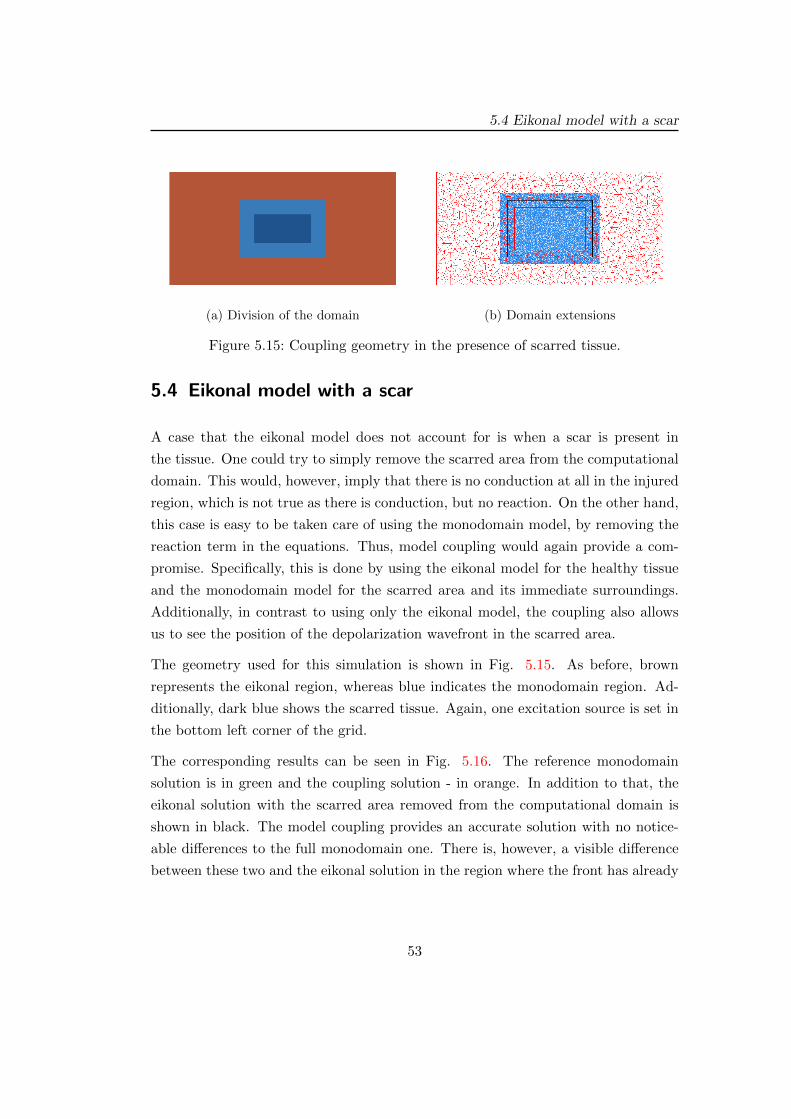
5.4 Eikonal model with a scar

(a) Division of the domain (b) Domain extensions

Figure 5.15: Coupling geometry in the presence of scarred tissue.

5.4 Eikonal model with a scar

A case that the eikonal model does not account for is when a scar is present in

the tissue. One could try to simply remove the scarred area from the computational

domain. This would, however, imply that there is no conduction at all in the injured

region, which is not true as there is conduction, but no reaction. On the other hand,

this case is easy to be taken care of using the monodomain model, by removing the

reaction term in the equations. Thus, model coupling would again provide a com-

promise. Specifically, this is done by using the eikonal model for the healthy tissue

and the monodomain model for the scarred area and its immediate surroundings.

Additionally, in contrast to using only the eikonal model, the coupling also allows

us to see the position of the depolarization wavefront in the scarred area.

The geometry used for this simulation is shown in Fig. 5.15. As before, brown

represents the eikonal region, whereas blue indicates the monodomain region. Ad-

ditionally, dark blue shows the scarred tissue. Again, one excitation source is set in

the bottom left corner of the grid.

The corresponding results can be seen in Fig. 5.16. The reference monodomain

solution is in green and the coupling solution - in orange. In addition to that, the

eikonal solution with the scarred area removed from the computational domain is

shown in black. The model coupling provides an accurate solution with no notice-

able differences to the full monodomain one. There is, however, a visible difference

between these two and the eikonal solution in the region where the front has already

53

5.4 Eikonal model with a scar

Figure 5.16: Wavefront position comparison for the full monodomain, model cou-pling and eikonal solutions in the presence of scarred tissue, with isolinesat 3 ms intervals (full monodomain - green, coupling - orange, eikonal -black).

(a) Division of the domain (b) Domain extensions

Figure 5.17: Coupling geometry in the presence of a very thin scarred tissue (fullmonodomain - green, coupling - orange, eikonal - white).

54

5.4 Eikonal model with a scar

passed the scarred tissue and also near the boundaries of the scar. Again, the eikonal

solution provides no results for the evolution of the depolarization wavefront in the

scarred tissue.

The difference is even more apparent when the scar is very thin, as in Fig. 5.17a,

where the scarred tissue is colored light gray. The results are shown in Fig. 5.17b,

with white representing the eikonal only solution, whereas, as before, the reference

monodomain solution is presented in green and the coupling solution - in orange. The

isolines obtained using only the eikonal model significantly lag behind the coupling

(and reference) solution. Although, due to the small area of the scar, its influence

on the wavefront should be minimal, the eikonal solution fails to provide accurate

results.

55

6 Conclusion

Two models for simulating the depolarization of cardiac cells have been presented.

The first one – the monodomain model – is represented by a parabolic partial dif-

ferential equation, coupled to ordinary differential equations that simulate the ionic

current. The approach developed by Aliev and Panfilov has been used as a model

for the ionic current, describing the excitation of cells as a propagating wavefront.

This model is both time and space dependent. Also, due to the small width of the

depolarization front, it requires a very fine spatial discretization.

The second – eikonal – model was derived from the first one, by making some

additional assumptions, in particular, that the shape of the upstroke does not change

significantly along the tissue. This allowed the elimination of the time variable, such

that the new eikonal model is only space dependent. It is described by a nonlinear

elliptic partial differential equation, that is much cheaper from a computational point

of view, but also slightly less accurate. Moreover, in contrast to the monodomain

model, it does not describe the shape of the wavefront, but only its position.

Numerical methods have been described for both models, the main ingredient being

the Finite Element Method. These methods motivate the need for coupling the

two models, i.e. using the monodomain model in the region where more accurate

results or the shape of the wavefront are needed, and the eikonal model elsewhere.

Conditions and algorithms for implementing this coupling for various situations have

been shown.

Numerical results for various geometries have then been presented. First, the validity

of the eikonal model has been demonstrated by comparing its results to the those

generated using the monodomain model. Then, results for the coupling in a simple

case with one excitation source have been presented. The collision of fronts was

also of interest, so a new source has been added in a further simulation. Finally,

56

as the eikonal model does not make provisions for the case when a scar in present

in the cardiac tissue, model coupling could be of use in this situation. Simulations

have been performed for this case as well. In order to determine the accuracy of the

coupling, all the results have been compared to reference solutions, obtained using

the monodomain model in the entire domain.

An obvious direction for further work on this topic is extending the coupling to more

irregular boundaries and to three spatial dimensions. In principle, the conditions

and algorithms would be the same. Irregular domains might require different meth-

ods of solving the eikonal model, as argued in [45], so a Petrov-Galerkin method

could be implemented. Additionally, one of the main issues in coupling the models

is that artificial boundaries are introduced, that do not exist otherwise. The solu-

tion is significantly affected in the vicinity of these new boundaries. Instead of the

approach used in this thesis of extending the domains, one could design transparent

boundary conditions for the two models. Further, an existing method for decreasing

the computational cost of the monodomain model is using mesh adaptivity [9, 16],

which could be used in the monodomain regions of the model coupling as well.

57

Bibliography

[1] R. R. Aliev and A. V. Panfilov. “A simple two-variable model of cardiac exci-

tation”. In: Chaos Solitons and Fractals 7 (3 1996), pp. 293–301.

[2] O. Axelsson and V. A. Barker. Finite Element Solution of Boundary Value

Problems: Theory and Computation. Academic Press, 1984.

[3] G. W. Beeler and H. Reuter. “Reconstruction of the action potential of ven-

tricular myocardial fibres”. In: The Journal of Physiology 268 (1 June 1977),

pp. 177–210.

[4] Y. Bourgault, Y. Coudiere, and C. Pierre. “Existence and uniqueness of the so-

lution for the bidomain model used in cardiac electrophysiology”. In: Nonlinear

Analysis: Real World Applications 10 (1 2009), pp. 458–482.

[5] M. R. Boyett et al. “Modelling cardiac excitation and excitability”. In: Com-

putational Biology of the Heart. Ed. by A. V. Panfilov and A. V. Holden. John

Wiley & Sons, 1997, pp. 1–47.

[6] P. Deuflhard, E. Hairer, and J. Zugck. “One-step and extrapolation methods

for differential-algebraic systems”. In: Numerische Mathematik 51 (5 1987),

pp. 501–516.

[7] P. Deuflhard. Newton Methods for Nonlinear Problems: Affine Invariance and

Adaptive Algorithms. Berlin Heidelberg: Springer Science & Business Media,

2004. Chap. 3.3, pp. 134–160.

[8] P. Deuflhard and F. Bornemann. Numerische Mathematik 2. German. Berlin,

New York: de Gruyter Lehrbuch, 2008. Chap. 6.4.2, pp. 295–298.

[9] P. Deuflhard and M. Weiser. Adaptive numerical solution of PDEs. Berlin,

Boston: De Gruyter, 2012.

58

Bibliography

[10] R. S. Eisenberg, V. Barcilon, and R. T. Mathias. “Electrical properties of

spherical syncytia”. In: Biophysical Journal 25 (1 1979), pp. 151–180.

[11] Electrophysiological Studies. Johns Hopkins Medicine. 2015. url: http://www.

hopkinsmedicine.org/healthlibrary/test_procedures/cardiovascular/

electrophysiological_studies_92,p07971/ (visited on 02/05/2016).

[12] F. Fenton and A. Karma. “Vortex dynamics in three-dimensional continu-

ous myocardium with fiber rotation: Filament instability and fibrillation”. In:

Chaos: An Interdisciplinary Journal of Nonlinear Science 8 (1 1998), pp. 20–

47. doi: http://dx.doi.org/10.1063/1.166311. url: http://scitation.

aip.org/content/aip/journal/chaos/8/1/10.1063/1.166311.

[13] R. A. FitzHugh. “Impulses and Physiological States in Theoretical Models of

Nerve Membrane”. In: Biophysical Journal 1 (6 1961), pp. 445–466.

[14] E. Flehmann et al. “Towards Patient Specific Catheter Selection: Computation

of Aortic Geometry Based on Fused MRI Data”. In: Functional Imaging and

Modeling of the Heart. Ed. by D. N. Metaxas and L. Axel. New York: Springer,

2011, pp. 145–152.

[15] P. C. Franzone, L. Guerri, and S. Rovida.“Wavefront propagation in an activa-

tion model of the anisotropic cardiac tissue: asymptotic analysis and numerical

simulations”. In: Journal of mathematical biology 28 (2 1990), pp. 121–176.

[16] P. C. Franzone et al.“ADAPTIVITY IN SPACE AND TIME FOR REACTION-

DIFFUSION SYSTEMS IN ELECTROCARDIOLOGY”. In: SIAM Journal

on Scientific Computing 28 (3 2006), pp. 942–962.

[17] S. Gotschel, M. Weiser, and A. Schiela. “Solving Optimal Control Problems

with the Kaskade 7 Finite Element Toolbox”. In: Advances in DUNE: Proceed-

ings of the DUNE User Meeting, Held in October 6th-8th 2010 in Stuttgart,

Germany. Ed. by A. Dedner, B. Flemisch, and R. Klofkorn. Berlin, Heidelberg:

Springer Berlin Heidelberg, 2012, pp. 101–112. isbn: 978-3-642-28589-9. doi:

10.1007/978-3-642-28589-9_8. url: http://dx.doi.org/10.1007/978-

3-642-28589-9_8.

[18] J. L. Greenstein, R. Hinch, and R. L. Winslow. “Mechanisms of excitation-

contraction coupling in an integrative model of the cardiac ventricular my-

ocyte”. In: Biophysical journal 90 (1 2006), pp. 77–91.

59

Bibliography

[19] J. L. Greenstein and R. L. Winslow. “An integrative model of the cardiac ven-

tricular myocyte incorporating local control of Ca2+ release”. In: Biophysical

journal 83.6 (2002), pp. 2918–2945.

[20] C. S. Henriquez. “Simulating the electrical behaviour of cardiac tissue using

the bidomain model”. In: Critical Reviews in Biomedical Engineering 21 (1

1993), pp. 1–77.

[21] A. L. Hodgkin and A. F. Huxley. “A quantitative description of membrane

current and its application to conduction and excitation in nerve”. In: The

Journal of Physiology 117 (4 1952), pp. 500–544.

[22] A. V. Panfilov and A. V. Holden, eds. Modelling propagation in excitable Media.

John Wiley & Sons, 1997, pp. 65–99.

[23] W. T. M. III and D. B. Geselowitz. “Simulation Studies of the Electrocardio-

gram”. In: Circulation Research 43 (2 1978), pp. 301–315.

[24] M. S. Jafri, J. J. Rice, and R. L. Winslow. “Cardiac Ca2+ dynamics: The

roles of ryanodine receptor adaption and sarcoplasmic reticulum load”. In:

Biophysical Journal 74 (3 1998), pp. 1149–1168.

[25] J. P. Keener. “A Geometrical Theory for Spiral Waves in Excitable Media”.

In: SIAM Journal on Applied Mathematics 46 (6 1986), pp. 1039–1056. doi:

10.1137/0146062. eprint: http://dx.doi.org/10.1137/0146062. url:

http://dx.doi.org/10.1137/0146062.

[26] B. Y. Kogan et al. “The simplified-FitzHugh-Nagumo model with action po-

tential duration restitution: effects on 2D wave propagation”. In: Physica D 50

(3 1991), pp. 327–340.

[27] W. Krassowska and J. C. Neu.“Effective boundary conditions for syncytial tis-

sues”. In: IEEE Transactions on Biomedical Engineering 41 (2 1994), pp. 143–

150.

[28] K. Kunisch, C. Nagaiah, and M. Wagner. “A parallel Newton-Krylov method

for optimal control of the monodomain model in cardiac electrophysiology”.

In: Computing and Visualization in Science 14 (6 2011), pp. 257–269.

60

Bibliography

[29] R. A. Luke et al. “Quantitative Analysis of Intercellular Connections by Im-

munohistochemistry of the Cardiac Gap Junction Protein Connexin43”. In:

Circulation Research 65 (5 1989), pp. 1450–1457.

[30] C. H. Luo and Y. Rudy. “A dynamic model of the cardiac ventricular action

potential”. In: Circulation Research 74 (6 1994), pp. 1071–1096.

[31] C. H. Luo and Y. Rudy. “A model of the ventricular cardiac action potential:

Depolarisation, repolarisation, and their interaction”. In: Circulation Research

68 (6 1991), pp. 1501–1526.

[32] R. E. McAllister, D. Noble, and R. W. Tsien. “Reconstruction of the electrical

activity of cardiac Purkinje fibres”. In: The Journal of Physiology 251 (1 1975),

pp. 1–59.

[33] S. Mendis et al. GLOBAL STATUS REPORT on noncommunicable diseases

2014. Report. World Health Organization, 2014. (Visited on 05/12/2015).

[34] D. Noble.“A modification of the Hodgkin-Huxley equations applicable to Purk-

inje fibre action and pace-maker potentials”. In: Journal of Physiology 160 (2

1962), pp. 317–352.

[35] D. Noble and R. L. Winslow. “Reconstructing the Heart: Network Models of

SA Node-Atrial Interaction”. In: Computational Biology of the Heart. Ed. by

A. V. Panfilov and A. V. Holden. John Wiley & Sons, 1997, pp. 49–64.

[36] D. Noble et al. “Improved guinea-pig ventricular cell model incorporating a

diadic space, IKr and IKs, and length- and tension-dependent processes”. In:

Canadian Journal of Cardiology 14 (1 1998), pp. 123–134.

[37] J. Roger and A. McCulloch. “A collocation-Galerkin finite element model of

cardiac action potential propagation”. In: IEEE Transactions on Biomedical

Engineering 41 (8 1994), pp. 743–757.

[38] Y. Saad. Iterative methods for sparse linear systems. 2nd ed. SIAM, 2003.

Chap. 10, pp. 301–321.

[39] F. B. Sachse. Computational cardiology. Berlin Heidelberg: Springer-Verlag,

2004. Chap. 6.1, pp. 120–56.

[40] F.-J. Sayas. A gentle introduction to the Finite Element Method. University of

Delaware. 2008.

61

Bibliography

[41] J. R. Shewchuk. “Triangle: Engineering a 2D Quality Mesh Generator and

Delaunay Triangulator”. In: Applied Computational Geometry: Towards Ge-

ometric Engineering. Ed. by M. C. Lin and D. Manocha. Vol. 1148. Lecture

Notes in Computer Science. From the First ACM Workshop on Applied Com-

putational Geometry. Springer-Verlag, 1996, pp. 203–222.

[42] Structure of the Heart. SEER Training Modules. U. S. National Institutes of

Health, National Cancer Institute. url: http://training.seer.cancer.

gov/anatomy/cardiovascular/heart/structure.html (visited on 01/26/2016).

[43] J. Sundnes et al. Computing the Electrical Activity in the Heart. Ed. by T. J.

Barth et al. Springer, 2006. Chap. 1.

[44] M. Thiriet and K. H. Parker. “Physiology and pathology of the cardiovascular

system: a physical perspective”. In: Cardiovascular Mathematics. Ed. by L.

Formaggia, A. Quarteroni, and A. Veneziani. MS&A. Milano: Springer-Verlag,

2009, pp. 1–46.

[45] K. A. Tomlinson. “Finite Element Solution of an Eikonal Equation for Exci-

tation Wavefront Propagation in Ventricular Myocardium”. Doctoral Thesis.

The University of Auckland New Zealand, 2000.

[46] L. Tung. “A bi-domain model for describing ischemic myocardial D-C poten-

tials”. Doctoral Thesis. Cambridge, Mass., USA: Massachusetts Institute of

Technology, 1978.

[47] Underlying Cause of Death 1999-2013 on CDC WONDER Online Database.

Center for Disease Control and National Center for Health Statistics. 2015.

url: http://wonder.cdc.gov/ucd-icd10.html (visited on 05/12/2015).

[48] H. A. van der Vorst. “Bi-CGSTAB: A Fast and Smoothly Converging Variant

of Bi-CG for the Solution of Nonsymmetric Linear Systems”. In: SIAM Journal

on Scientific and Statistical Computing 13 (2 1992), pp. 631–644.

[49] H. Wardhan and S. Singh. “Modeling of generation and propagation of cardiac

action potential using fractional capacitance”. In: IOSR Journal of Biotech-

nology and Biochemistry 1 (2 2015), pp. 1–11.

62

Bibliography

[50] N. Wiener and N. Rosenbluth. “The mathematical formulation of the problem

of conduction of impulses in a network of connected excitable elements, specif-

ically in cardiac muscle”. In: Archivos del Instituto de Cardiologia de Mexico

16 (3 1946), pp. 205–265.

[51] R. L. Winslow et al. “Mechanisms of altered excitation-contraction coupling

in canine tachycardia-induced heart failure, II, model studies”. In: Circulation

Research 84 (1999), pp. 571–586.

[52] D. W. Zhu et al. “The Value of Electrophysiology Study and Prophylactic

Implantation of Cardioverter Defibrillator in Patients with Hypertrophic Car-

diomyopathy”. In: Pacing and Clinical Electrophysiology 21 (1 1998).

63