EINDHOVEN UNIVERSITY OF TECHNOLOGY Department of Mathematics and Computer Science

CASA-Report 13-35 December 2013

Experimental investigation on rapid filling of a large-scale pipeline

by

Q. Hou, A.S. Tijsseling, J. Laanearu, I. Annus, T. Koppel, A. Bergant, S. Vučkovič, A. Anderson, J.M.C. van ’t Westende

Centre for Analysis, Scientific computing and Applications

Department of Mathematics and Computer Science

Eindhoven University of Technology

P.O. Box 513

5600 MB Eindhoven, The Netherlands

ISSN: 0926-4507

Experimental Investigation on Rapid Filling of a Large-Scale Pipeline

Qingzhi Hou, Dr., SKLHESS, School of Civil Engineering;School of Computer Science and Technology, Tianjin University,

300072 Tianjin, China (corresponding author). E-mail: qhou@tju.edu.cnArris S Tijsseling, Dr., Department of Mathematics and Computer Science, Eindhoven

University of Technology, P.O. Box 513, 5600 MB Eindhoven, The Netherlands.Janek Laanearu, Dr., Department of Mechanics, Tallinn University of

Technology, Ehitajate tee 5, 19086 Tallinn, Estonia.Ivar Annus, Dr., Department of Mechanics, Tallinn University of Technology,

Ehitajate tee 5, 19086 Tallinn, Estonia.Tiit Koppel, Prof., Department of Mechanics, Tallinn University of Technology,

Ehitajate tee 5, 19086 Tallinn, Estonia.Anton Bergant, Dr., Litostroj Power d.o.o., Litostrojska 50, 1000 Ljubljana, Slovenia.Saso Vuckovic, Mr., Litostroj Power d.o.o., Litostrojska 50, 1000 Ljubljana, Slovenia.Alexander Anderson, Senior Lecturer, School of Mechanical and Systems Engineering,

Newcastle University, Newcastle upon Tyne NE1 7RU, United Kingdom.Jos M C van ’t Westende, Dr., Deltares, P.O. Box 177, 2600 MH Delft, The Netherlands.

ABSTRACTThis study presents results from detailed experiments of the two-phase pressurized flow behavior

during the rapid filling of a large-scale pipeline. The physical scale of this experiment is closeto the practical situation in many industrial plants. Pressure transducers, water level meters,thermometers, void fraction meters and flow meters were used to measure the two-phase unsteadyflow dynamics. The main focus is on the water-air interface evolution during filling and the overallbehavior of the lengthening water column. It is observed that the leading liquid front does notentirely fill the pipe cross section; flow stratification and mixing occurs. Although flow regimetransition is a rather complex phenomenon, certain features of the observed transition pattern areexplained qualitatively and quantitatively. The water flow during the entire filling behaves as arigid column as the open empty pipe in front of the water column provides sufficient room for thewater column to occupy without invoking air compressibility effects. As a preliminary evaluationof how these large-scale experiments can feed into improving mathematical modeling of rapid pipefilling, a comparison with a typical one-dimensional rigid-column model is made.

Keywords: Experimentation; Large-scale pipeline; Two-phase flow; Air-water interface; Flow-regime transition

INTRODUCTIONRapid pipe filling occurs in various hydraulic applications, such as water-distribution networks,

storm-water and sewage systems, fire-fighting systems, oil transport, and pipeline cleaning andpriming. While the water column is driven by a high head, air is expelled by the advancing watercolumn. If the generated air flow is not blocked by obstacles, such as gates, valves or orifices,the water column grows with little adverse pressure and may attain a high velocity. When theadvancing column is suddenly stopped (fully or partially), severe pressure changes will occur in thesystem (see e.g. Guo and Song 1990, De Martino et al. 2008, Bergant et al. 2010, Bergant et al.2011, Martin and Lee 2012).

Rapid filling processes in single pipes have been studied experimentally before. Nydal andAndreussi (1991) investigated the air entrainment in a water column advancing over a liquid film

1

in a nearly horizontal pipe that was 17 m long and 50 mm in diameter. It was found that airentrainment only occurred when the relative velocity between the advancing front and the liquidlayer was greater than a threshold 2D/Wi (Wi interfacial width). When there was no initial liquidfilm in the pipe, air entrainment did not occur. Liou and Hunt (1996) investigated the rapid fillingof a 7 m long pipe with a diameter of 23 mm. A high but short-lived peak velocity occurred afterwhich the velocity slowly decreased to its steady state value. To check the validity of the planarfront assumption in the rigid-column model of Liou and Hunt (1996), Vasconcelos et al. (2005)studied the filling process of a 14 m long and 94 mm diameter pipe for three different drivingheads. It was observed that the advancing water column did not entirely fill the pipe cross section,and a stratified flow was observed behind the leading front.

In the context of pipe filling, the usual focus was on physical factors affecting the peak transientpressure, such as the location and size of entrapped air pocket(s), the water column length, thedriving pressure head and the size of the end orifice (Martin 1976, Ocasio 1976, Cabrera et al. 1992,Cabrera et al. 1997, Izquierdo et al. 1999, Lee and Martin 1999, Zhou 2000, Liu and Suo 2004,Lee 2005, De Martino et al. 2008, Zhou et al. 2011, Martin and Lee 2012, Zhou et al. 2013a, Zhouet al. 2013b). Ocasio (1976) carried out experiments with entrapped air pockets at a dead end anddemonstrated that the presence of entrapped air could result in destructive pressure surges. This isconsistent with the conclusions drawn by Martin (1976). Lee and Martin (1999), Zhou (2000) andLee (2005) investigated the effect of relatively large entrapped air pockets (initial void fractionsbetween 6% and 45%) in horizontal pipelines with dead ends. They found that the maximumpeak pressure of the air pocket increased with the decrease of its initial size. As a complementarywork, Zhou et al. (2011) presented experimental measurements in an undulated pipeline with smallinitial void fraction (from 0 to 10%). They found that the maximum peak pressure of the air pocketfirst increased and then decreased with decreasing void fraction. For the filling of pipelines withundulating profile, multiple air pockets and an open end, the rapid compression of the entrappedair may cause huge pressures (Cabrera et al. 1997, Izquierdo et al. 1999, Zhou et al. 2013a). Whentwo air pockets are entrapped, the case with similar sizes was the most complicated and dangerousone (Zhou et al. 2013a). To investigate the behavior of the air entrapped in a drainage system,Yamamoto et al. (2000) presented an experimental study that involved the use of a horizontal pipewith a length of 122 m and a diameter of 200 mm. The entrapped air increased both the pressurerise time and the pressure peak. Zhou et al. (2002) investigated the rapid filling of a horizontalpipe with an end orifice which was partially full with water. The pipe length was 9 m and thediameter was 35 mm. The focus was on pressure surge influenced by the initial water depth, theorifice size, and the driving head. It was demonstrated that air trapped in a rapidly filled pipecan induce high-pressure surges, especially when air leakage occurred at the orifice. Three typesof pressure oscillation patterns were observed, depending on the size of the orifice. Recently, toascertain the effect of entrapped air and orifice size on pipeline transients, a similar experimentaltest programme was reported by Martin and Lee (2012) with results similar to those in Yamamotoet al. (2000).

To study the transition from free surface to pressurized flow in sewers during storm events, Tra-jkovic et al. (1999) conducted experiments in a test rig consisting of a circular pipe with downwardslope and gates at the upstream and downstream ends. The overall pipe length was about 10 mand the pipe diameter was 100 mm. It was found that the supercritical free-surface flow at theupstream end (under proper ventilation) always induced a hydraulic jump. Recently, inspired bythe work of Trajkovic et al. (1999), a similar experimental investigation was conducted by Trindadeand Vasconcelos (2013) with modifications that limited the ventilation conditions. For the studyof flow regime transition and the interaction between air and water phases, Vasconcelos (2005) andVasconcelos and Wright (2005) conducted rapid filling experiments of a poorly ventilated stormwa-

2

ter tunnel. The pipe was initially empty or partially filled with water. It was found that the airnear the pipe crown could pressurize and influence the flow dynamics. The surge intensity wasmaximized when a hydraulic bore propagated towards the surge riser (also observed by Nydal andAndreussi 1991), and it increased with the pressure head behind the pressurization front. In thisrespect, the current paper provides useful experimental information complementary to the previousstudies on pipeline filling.

These previous studies show that for filling of a small-scale horizontal system with relativelyhigh driving head, the deformation of the water front has an insignificant effect on the overallhydrodynamics of the lengthening water column (Hou et al. 2012b). Thus a planar water-airinterface is often assumed. However, it is not clear in advance whether this assumption is applicableto large-scale pipelines. This issue is of high importance to understand the development of airpockets and gravity currents during the filling process. The present experimental investigationaims at a better understanding of the evolution of the moving interfaces, the pressure distributionand the flow rates. To assist in interpreting the experimental results they are compared withpredictions from a one-dimensional model which has the conventional planar water-air interfaceassumption. This paper complements the experimental work done in the same Deltares pipelineapparatus on the emptying of it by different upstream compressed-air pressures and with differentoutflow restriction conditions (Laanearu et al. 2012).

EXPERIMENTAL APPARATUSThe experimental apparatus consisted of a water tank, an air tank, steel supply pipelines (for

water and air), a PVC inlet pipe, a pipe bridge, a horizontal long PVC pipeline (the test section),an outlet steel pipeline and a basement reservoir. Detailed information is given below, and part ofit can be found in Lubbers (2007), Laanearu et al. (2009, 2012), Laanearu and van ’t Westende(2010) and Hou (2012). The downstream end of the PVC pipe bridge was defined as the origin ofthe coordinate system. It is the starting point of the test section. The x -coordinate follows thecentral axis of the pipeline, the y-coordinate is not used herein and the z-coordinate is the verticalelevation. Coordinates of measuring instruments and other important components are shown inFig. 1.

A water tank with a constant 25 m head relative to the center line of the inlet (x = −34.6 m) wasused to supply water in the filling experiment reported here and an air tank with a 70 m3 volumewas used to supply air in the emptying experiment (Laanearu et al. 2012). The horizontal inlet steelpipe from the tank to the vertical leg was 2.6 m long. The vertical leg of the Y-junction was 3.6m long. The steel pipe, from the Y-junction (x = −27.2 m) to the upstream steel-PVC connection(x = −14 m), was 13.2 m long. The air supply steel pipe, from the check valve (x = −43.1 m) tothe Y-junction, was 15.9 m long. The inner diameter of the steel pipes was 206 mm, with a wallthickness of 5.9 mm. The PVC pipe was 275.2 m long and its outer diameter was 250 mm withan average wall thickness of 7.3 mm. It consisted of two parts. The first part consisted of a 7.5 mlong PVC inlet pipe and a 6.5 m long pipe bridge. It led from the upstream steel-PVC connection(x = −14 m) to the chosen starting point of the test section (x = 0). With the aid of a piezometertube, the bridge was used to set up the initial water column. The second part was the horizontalPVC pipe of length 261.2 m (from x = 0 to the downstream PVC-steel connection). Most of themeasurements took place in this section. The outlet steel pipe led from the downstream end of thePVC pipe to the basement reservoir. It contained two segments of different diameter connectedby a reducer. The reducer had a length of 0.3 m and was located 0.3 m upstream of the outletflow meter. The first segment was 8.8 m long and the inner diameter was 260.4 mm with a wallthickness of 6.3 mm. The second segment was 2 m long and the inner diameter was 206 mm witha wall thickness of 5.9 mm. The pipeline had downward turns at x = −27.2 m and x = 267.0 m,

3

FIG. 1. System dimensions and coordinates of the measuring instruments adapted from Bergantet al. (2011).

4

and an upward turn at x = −31.6 m. The elevation information is given in Fig. 1. The downwardleg beyond x = 267.0 m formed a siphon after the water front arrived at the last elbow.

Pipe supports and connections

To suppress pipe motion and associated Fluid-Structure Interaction (FSI) effects (see e.g.Bergant et al. 2010, Bergant et al. 2011, Keramat et al. 2012, Tijsseling 1996, Wiggert and Tijssel-ing 2001), it was attempted to structurally restrain the pipe system as much as possible. The PVCpipeline was fixed to the concrete floor by metal anchors and supported with wooden blocks toreduce sagging. The pipe bridge – elevated 1.3 m above the main pipeline axis – was supported bya tube-frame. As it appeared hard to fix the most downstream elbow (x = 267.0 m), a heavy mass(about 1 tonne) was attached with a rope at this point so to reduce the elbow’s vertical movement.The PVC pipeline segments were connected by sleeves. Wherever the PVC pipe needed to changedirection, a large-radius bend (R = 5DPV C) was used. There were four 90-degree bends in the testsection and a long bend at the 180 degree turning point (see Fig. 1).

There were nine valves in the system as indicated in Fig. 1. Several small air venting valvesare not shown; most of the venting valves were located upstream of the pipe bridge. All of themwere closed in the filling process, which is different from the upstream ventilation condition usedin the filling tests by Trajkovic et al. (1999) (full ventilation) and Trindade and Vasconcelos (2013)(limited ventilation). The check valve (V7 at x = −43.1 m) was used to prevent entrance of waterinto the air system. The water inlet valve (V8 at x = −34.6 m) connected to the water tankremained open during all experiments. The other seven valves labeled V0 to V6 were activelyoperated manually or automatically (see Fig. 1). Three of them (V0, V2 and V6) were used in thefilling tests. The upstream service valve V0 (DN200) was operated manually to supply water. Theautomatic control valve V2 (DN150) was used for flow regulation. The small-size on/off valve V6in the transparent stand tube mounted at the upstream leg of the pipe bridge (see Fig. 1) was openwhen monitoring the initial position of the front of a nearly static water column. All the watervalves used in the system were butterfly valves and the check valve (V7) was a cage valve.

Instruments and data acquisition

Instruments. A maximum of 29 instruments were installed along the whole system as sketchedin Fig. 2. There were twelve pressure transducers, six water level meters, four thermometers,three void fraction meters, three flow meters and one accelerometer. The coordinates of the pres-sure transducers and flow meters are shown in Fig. 1. The coordinates of the other measuringinstruments can be found in Hou et al. (2012a), where the type, output range, position (withinpipe cross-section) and other relevant information is provided. The three transparent sections hadlengths of 0.7 meters with viewing windows 0.5 meters long. A SONY camera set-up at the firstand last sections (see Fig. 2) recorded the water-air interfaces and the air-water mixing process.The nine measuring sections were numbered (indicated by the subscripts of variables in Figs. 1 and2) in sequence from upstream to downstream.

Uncertainties. According to nominal values provided by the manufactures, the estimated uncer-tainty under steady-state conditions was ± 1.0% (percent of reading) in the flow-rate measurements,± 0.1% (percent of reading) in the pressure measurements and ± 0.8 oC in the temperature mea-surements. The ± 15 mm uncertainty in the water-level measurements was not known from theinstrumentation specification of the conductivity probe, but it was determined from comparisonswith camera images. All pressure transducers were of the strain-gauge type with a natural frequen-cy of 10 kHz. They were all installed flush-mounted at the pipe sides, except for p3. Apart fromthe uncertainties in the measuring devices, there were also uncertainties in the filling process itself.

• The response times of the measuring instruments were different. For example, for the pres-

5

FIG. 2. Layout of measuring instruments in the pipeline apparatus.

sure transducer and the flow meter located at the same place, the response of the pressuretransducer was normally 1 second earlier than the response of the flow meter. The instantof the first response of the flow meter at x = −14 m was taken as time t = 0.

• The PVC pipeline was intended to be entirely empty before each pipe filling run. However,it was found that some water remained between the sections 3 (x = 46.4 m) and 8 (x = 206.8m) after a filling and subsequent emptying run. The amount of uncleared water varied pertest. With valve V4 fully open and using high-pressure air (more than 1 bar) to drain thepipe, the depth of remaining water was about 30 mm on average and up to 60 mm when airat low-pressure (less than 1 bar) was used. The experimental results examined herein wereobtained after draining with high-pressure air. For the average depth of 30 mm (betweensections 3 and 8), the volume of the remaining water is 0.52 m3 which is equivalent to thevolume of 12 m of the PVC pipe.

• Before each pipe filling run, the air entrapped in the steel pipe between the Y-junction(x = −27.2 m) and the check valve (x = −43.1 m) was not released. It is not clear what itseffect is on the filling process in general and air entrainment in particular.

Data acquisition. Deltares’ 32-channel data acquisition system was used for synchronized record-ing of flow rate (inflow Qu, outflow Qdv, air flow Qa), pressure (p1, p3t, p3b, p5, p7, p8, p9, pu, puv,pdv, pa, pt), temperature (T1, T3, T9, Ta), water level (WL1, WL3, WL5, WL7, WL8, WL9) andvoid fraction (VF1, VF3, VF9); see Fig. 2. Video camera and accelerometer recordings were notelectronically synchronized with the data acquisition recordings. The camera images were highlyuseful to get direct visual information on the two-phase flow structure developing in the pipe. Asampling rate of 100 Hz was used to record discharge, gauge pressure, water level, void fractionand temperature.

6

−50 0 50 100 150 200 250−5

0

5

10

15

20

25

Locations (m)

Hea

d (m

)

FIG. 3. Steady-state hydraulic grade line.

Test procedure

All pipe filling experiments were carried out with the downstream valves V4 and V5 fully openand a constant driving head of 25 m (at x = −34.6 m, z = −3.6). Air at atmospheric pressure andsome stagnant water is initially present in the system. First, the upstream valve V0 was openedmanually. Then the automatic valve V2 was opened from 0 to 15% until the height of the water inthe pipe bridge reached a vertical level of 0.4 meter (0.04 barg reading from pressure transducer puat x = −14 m as shown in Fig. 1). After closing valve V2, the water level at x = −6.5 m (which isat the upstream leg of the bridge) was allowed to reach the level of 1.0 m (visually observed fromthe piezometer tube) gradually due to a small leakage of valve V2. When this level was reached,the upstream pipe was full and the top of the bridge was empty. Filling then started by closingthe small valve V6 on the piezometer tube and by fully opening valve V2 at the same time. Thefilling was rapid, within one minute time. After that a steady state was reached, i.e. the inlet andoutlet flow discharges were equal and constant, the outlet control valve V4 was closed slowly byhand from 0 to 75 degrees (labeled on a panel) to avoid any pressure surges. After the gradualclosure of valves V5 and V2 the filling process was completed.

EXPERIMENTAL RESULTS

Steady-state friction and resistance

Prior to the rapid pipe filling experiments, full-pipe steady-flow measurements were carried outto determine the system’s head loss characteristics. At a steady-state flow velocity of 4 m/s thehydraulic grade line for the PVC pipe is shown in Fig. 3. The straight hydraulic grade line forx > 0 confirms that the pipe test section was long enough to neglect the minor losses due to thebends (necessary to accommodate the pipe length within the laboratory). Laanearu et al. (2012)have shown that the steady-state friction factor of the test pipe was f = 0.0136 and the 180o turnloss coefficient was Klb = 0.06. The friction head loss over the L = 275.2 m PVC pipe was hf = 13m, in comparison with which the local head loss hlb = 0.05 m due to the 180o turn was negligible.The large head loss in the upstream part of the pipeline from x = −34.6 m to x = −27.7 m wasmainly due to the resistance of the valves V0, V2 and V8.

7

0 20 40 60 80 100

0

50

100

150

200

250

Time (s)

Flo

w r

ate

(L/s

)

Run 1Run 2Run 3

inflow outflow

FIG. 4. Measured inflow and outflow rates in three typical pipe filling runs.

Flow rates

The upstream and downstream flow rates measured during filling are shown in Fig. 4, wheregood repeatability is exhibited by the three representative runs. The arrival time of the watercolumn at the downstream flow meter (x = 270.3 m) is 54± 0.8 s. The area covered by the inflowrate curve and the time-axis between t = 0 and t = 54 s is the amount of water that has beenfed into the pipeline. The estimated value is 11,150 liters. It is less than the empty pipe volume∀ = AL = πD2

PV C/4 × (270.3 + 6.5) × 103 = 12, 000 liters (water column front starts at x = −6.5m), from which the volume of water present before filling (about 500 liters) must be subtracted.The volume discrepancy of 350 liters is equivalent to the volume of 8 m length of PVC pipe. Thisimplies that when the water column arrives at the downstream flow meter, not all air is expelledout of the system. This matter is further examined in the next section.

Now we focus on the measurements by the upstream flow meter (x = −14 m). As shownin Fig. 4, the flow rate first rises to its maximum value of 270 ± 3 l/s in about 4 seconds time.Then it decreases rapidly from 270 l/s to 250 l/s in 2 seconds time. After that, the flow graduallydecelerates until a steady state of fully-filled pipe flow is reached with short-living water-hammerdue to slug impact (see Fig. 11). The inflow velocity V – determined from the averaged flow rateof 9 runs – is shown in Fig. 5 by the solid line. The trend of the curve is the same as that in thesmall-scale experiment of Liou and Hunt (1996), although the filling time is over 11 times longerhere (about 57 seconds versus 5 seconds) mainly due to the longer pipe length. The measuredmaximum velocities are higher (about 6.2 m/s versus 1.6 m/s) mainly due to the higher drivinghead in the present experimental setup.

Water-air interfaces

Since the initial static water front (water-air interface) splits into two water fronts during thefilling process, the sketch in Fig. 6 is introduced for the sake of clarity. To determine the waterfront velocities V1 (leading front) and V2 (secondary front) (Fig. 6c), the measuring method of Liouand Hunt (1996) is used. Two different groups of instruments are used as the front timing sections.The first group consists of the six water level meters (WL1, WL3, WL5, WL7, WL8 and WL9)located at x = 1.7, 46.4, 111.7, 183.7, 206.8 and 252.9 m, respectively. The second group consists

8

0 20 40 60 80 100

0

1

2

3

4

5

6

Time (s)

Vel

ocity

(m

/s)

V2

V

V1

FIG. 5. Velocity history of the inflow and the water fronts in the filling experiments. Solid line– adapted from upstream flow measurements; symbols – indirect measurements (squares – V1

– leading front, diamonds – V2 – secondary front).

FIG. 6. Water front evolution in the filling process – the original water front splits into twofronts: (a) initial state, (b) early stage of filling and (c) propagation of two water fronts.

of the six pressure transducers (p1, p3b, p5, p7, p8 and p9) located at x = 1.6, 46.6, 111.7, 183.7,206.8 and 252.8 m. Except for pressure transducer p3b which is located at the pipe bottom, theother five transducers are in a horizontal plane with the pipeline axis. The water level meters arein a vertical plane with the pipeline axis. The arrival times of the advancing water fronts at thetiming sections are captured by the two groups of instruments. The average speeds of the frontsare then computed as the distances between the timing sections divided by the travel times.

Together with the inflow velocity, the measured water front velocities are shown in Fig. 5: thesquares indicate V1 and the diamonds V2. The velocities V1 and V2 are average velocities over thetrajectory between two subsequent sections and the symbols are plotted at the arrival times of

9

TABLE 1. Location x, arrival time t, average velocity V1 and inflow velocity V (at t1) of theleading water front. The unit for x, t and V is m, s and m/s, respectively.

Section x t1 V1 V V1 − V

1 1.7 1.61± 0.07 5.09 2.61 2.483 46.4 9.12± 0.16 5.96 5.66 0.305 111.7 21.09± 0.36 5.46 5.05 0.417 183.7 35.28± 0.33 5.07 4.50 0.438 206.8 40.20± 0.35 4.70 4.36 0.249 252.9 50.34± 0.44 4.55 4.10 0.45

TABLE 2. Location x, arrival time t, average velocity V2 and inflow velocity V (at t2) of thesecondary water front. The unit for x, t and V is m, s and m/s, respectively.

Section x t2 V2 V V − V2

1 1.7 5.44± 0.18 1.38 5.84 4.463 46.4 14.51± 0.25 4.92 5.30 0.385 111.7 32.48± 0.40 3.63 4.56 0.967 183.7 56.17± 0.59 3.04 4.00 0.968 206.8 64.39± 0.36 2.81 4.06 1.259 252.9 80.42± 0.41 2.87 4.03 1.16

the water fronts at the timing sections. Only velocities determined from the water level metersare presented in Fig. 5. The pressure transducers gave results close to those from the water levelmeasurements for the leading front (V1), whilst they could not accurately sense the arrival of thesecondary front (V2) due to the small pressure rise associated with it. The water front starts atx = −6.5 m and has already split into two fronts when it arrives at section 1 (x = 1.7 m) sothat velocities V1 and V2 are clearly different and the difference is more than 1 m/s as seen fromFig. 5. Both water front velocities follow the trend of the inflow rate. The front arrival times attiming sections and corresponding velocities are listed in Tables 1 and 2. When the leading frontis traveling between section 3 (x = 46.4 m) and section 9 (x = 252.9 m), the velocity differencebetween water column front (V1) and tail (V ) is roughly 0.4 m/s, except at section 8 (x = 206.8m) where it decreases to 0.24 m/s. Similarly, before the secondary front arrives at section 9, thevelocity difference between front (V2) and tail (V ) is about 1 m/s except at section 8 (x = 206.8m), where the difference increases to 1.25 m/s due to air pocket formation. The velocity variationat section 8 is because of a hydraulic jump that occurred between sections 8 and 9, which is evidentfrom the water level measurements shown below. The area between the velocity curves V1 andV2 (interpolated from Tables 1 and 2) is the amount of air intruded on top of the stratified flow.This is further examined at the end of the next section. Two water fronts were also observed byVasconcelos et al. (2005) and presented by Guizani et al. (2006), however, without a quantitativeanalysis as made herein.

10

Water levels

The water level measurements for three repeated runs in Fig. 7 show a good repeatability. Thesplitting of the water front is evident. The water levels at six locations in one typical run are shownin Fig. 8. It is clear from Figs. 7 and 8 that the pipeline is not entirely empty at the beginning.Water is mainly present between section 3 (x = 46.6 m) and section 8 (x = 206.8 m), and itshighest level is 35 mm at section 5 (x = 111.7 m). The fact that there is water accumulation inthe system prior to the filling is possibly due to the sagging of the pipeline. That is, the elevationof the pipeline between sections 3 (x = 46.6 m) and 8 (x = 206.8 m) is not zero as desired, but asmall negative value. This condition differs from rapid filling tests with sloped pipelines as used byLiou and Hunt (1996) and Vasconcelos et al. (2005). As indicated by Arai and Yamamoto (2003),the pipeline slope could locally deviate from the targeted slope.

Figure 8 indicates that the shape of the leading water front does not change much before itarrives at section 9 (x = 252.9 m). Its final wedge length is about 3 meters as estimated from theobserved rise time (0.5 – 0.75 s) and the measured velocity. The wedge-shaped front (see Figs. 8and 6c) is initiated at the pipe bridge. As Fig. 7 shows, the water surface of the stratified flowis fluctuating (small burrs in Figs. 7e and 7f and large spikes in Figs. 7a and 7d) caused by localobstructions, such as bridge and bends. This is consistent with the observation of Hamam andMcCorquidale (1981) that even if there was no hydraulic jump in the sewer, the water surfacewas very unstable at relative depths h/D > 0.8, showing that the stratified flow was affected bygeometric discontinuities.

However, for the long-time behavior, the average height of the leading water front is more orless constant (192±8 mm) until it arrives at section 9 (x = 252.9 m) where it increases to 230 mm.The secondary front reaches section 1 (x = 1.7 m) at about t = 5.4 s. Its shape slightly changeswith time. The average height of the secondary front is 43 ± 8 mm until it arrives at section 8(x = 206.8 m). It decreases to 6 mm at section 9 (x = 252.9 m). The abrupt change of the heightof the two water fronts at section 9 indicates that a large flow regime transition (hydraulic jump)must have occurred between sections 8 (x = 206.8 m) and 9 (x = 252.9 m). The occurrence of ahydraulic jump is attributed to the 90-degree elbow and the stagnant layer of water ahead of theleading water front. The distance between the two water fronts ∆L = (V1 − V2)∆t increases withtime. It is about 20 m when the secondary water front arrives at x = 1.7 m (t = 5.4 s), and itincreases to 75 m when the leading water front arrives at x = 206.8 m at t = 40.2 s. According tothese observations, a quantitative analysis of the water-air interface evolution is sketched in Fig. 9.

Due to insufficient draining between two subsequent filling tests, most part of the pipeline hasan initial water depth (mainly from x = 46.4 m to x = 206.8 m and depth varying with the xcoordinate). Generally, a sudden inflow in such a system will generate a bore (planar) front andnot a feather-tip (wedge) front like the one indicated in Fig. 6. However, the images captured bythe camera (see Fig. 10) did not indicate a clear bore front. This is attributed to the pipe bridge,which produces a wedge-shaped front straight away, and to the relatively small water depth (lessthan 5% of the pipe diameter as shown in Fig. 7f) at the measuring site (x = 249.5 m, close tosection 9). The images captured at the transparent location (x = 3.8 m) are similar to those shownin Fig. 10 but with a higher evolution speed. A recording at the transparent location (x = 68.5m in Fig. 1) would have provided useful insights in this respect, but unfortunately this has notbeen done due to a lack of time. However, when zooming in on Fig. 7, the measured water levelrise caused by the leading water front at positions with relatively large initial water depth (e.g.x = 111.7 m and x = 183.7 m) is still a sort of linear wedge. The sampling rate of 100 Hz used inthe experiments was sufficiently high to capture a planar bore front if it were there.

The evolution of the leading water front involves the intrusion of air. When the leading water

11

1 2 3 4 5 60

50

100

150

200

250

Time (s)

Wat

er le

verl

(mm

)

(a) WL1

Run 1Run 2Run 3

9 10 11 12 13 14 150

50

100

150

200

250

Time (s)

Wat

er le

verl

(mm

)

(b) WL3

Run 1Run 2Run 3

20 22 24 26 28 30 32 340

50

100

150

200

250

Time (s)

Wat

er le

verl

(mm

)

(c) WL5

Run 1Run 2Run 3

35 40 45 50 550

50

100

150

200

250

Time (s)

Wat

er le

verl

(mm

)

(d) WL7

Run 1Run 2Run 3

40 45 50 55 60 650

50

100

150

200

250

Time (s)

Wat

er le

verl

(mm

)

(e) WL8

Run 1Run 2Run 3

50 55 60 65 70 75 80 850

50

100

150

200

250

Time (s)

Wat

er le

verl

(mm

)

(f) WL9

Run 1Run 2Run 3

FIG. 7. Water levels at six different locations in three repeated filling runs: (a) WL1, (b) WL3,(c) WL5, (d) WL7, (e) WL8 and (f) WL9. See Table 1 and Fig. 2 for locations.

12

0 10 20 30 40 50 60 70 80 900

50

100

150

200

250

Time (s)

Wat

er le

verl

(mm

)

WL1WL3WL5WL7WL8WL9

FIG. 8. Water level changes at six different locations in one typical filling run.

FIG. 9. Illustration of air intrusion in the filling experiments (unit: m). The layer of intrudedair lengthens while its thickness does not change in stages (b), (c), (d) and (e). A hydraulicjump occurred between stages (e) and (f), after which entrapped air is gradually expelled fromthe system.

13

FIG. 10. Water front evolution at x = 249.5 m in the filling process – snapshots by videocamera with a 0.04 s time interval starting at t = 50 s.

14

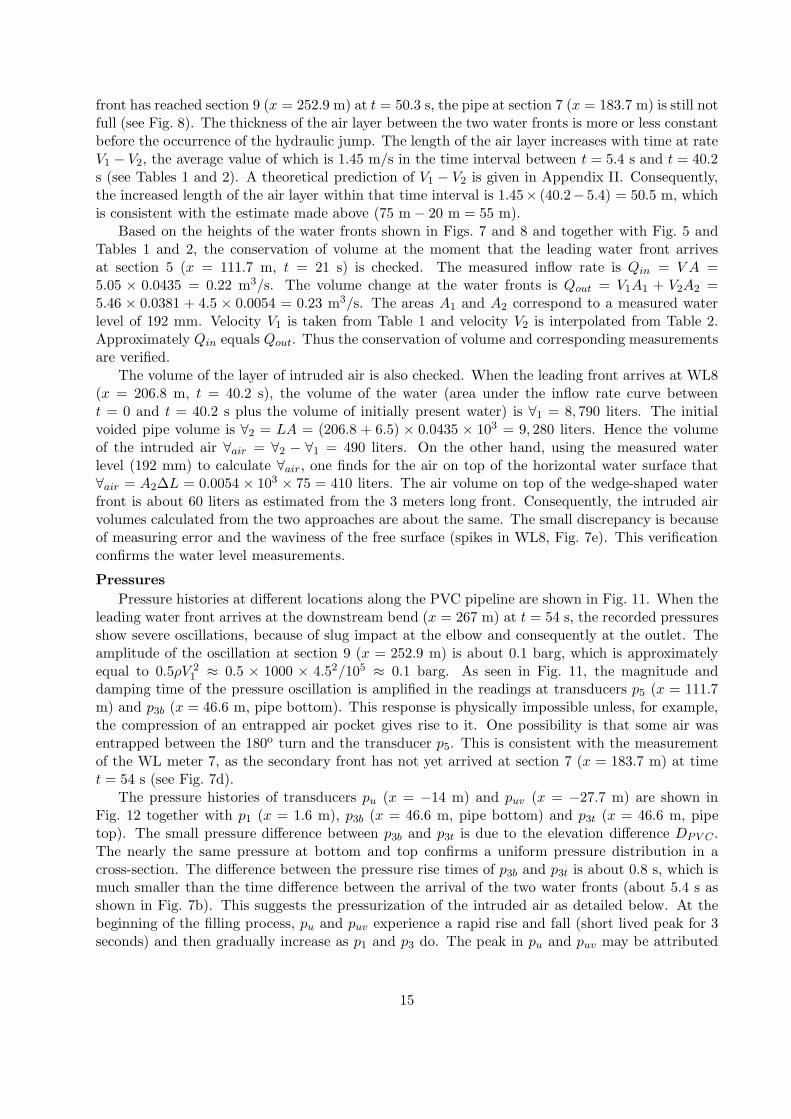
front has reached section 9 (x = 252.9 m) at t = 50.3 s, the pipe at section 7 (x = 183.7 m) is still notfull (see Fig. 8). The thickness of the air layer between the two water fronts is more or less constantbefore the occurrence of the hydraulic jump. The length of the air layer increases with time at rateV1 − V2, the average value of which is 1.45 m/s in the time interval between t = 5.4 s and t = 40.2s (see Tables 1 and 2). A theoretical prediction of V1 − V2 is given in Appendix II. Consequently,the increased length of the air layer within that time interval is 1.45× (40.2− 5.4) = 50.5 m, whichis consistent with the estimate made above (75 m− 20 m = 55 m).

Based on the heights of the water fronts shown in Figs. 7 and 8 and together with Fig. 5 andTables 1 and 2, the conservation of volume at the moment that the leading water front arrivesat section 5 (x = 111.7 m, t = 21 s) is checked. The measured inflow rate is Qin = V A =5.05 × 0.0435 = 0.22 m3/s. The volume change at the water fronts is Qout = V1A1 + V2A2 =5.46 × 0.0381 + 4.5 × 0.0054 = 0.23 m3/s. The areas A1 and A2 correspond to a measured waterlevel of 192 mm. Velocity V1 is taken from Table 1 and velocity V2 is interpolated from Table 2.Approximately Qin equals Qout. Thus the conservation of volume and corresponding measurementsare verified.

The volume of the layer of intruded air is also checked. When the leading front arrives at WL8(x = 206.8 m, t = 40.2 s), the volume of the water (area under the inflow rate curve betweent = 0 and t = 40.2 s plus the volume of initially present water) is ∀1 = 8, 790 liters. The initialvoided pipe volume is ∀2 = LA = (206.8 + 6.5) × 0.0435 × 103 = 9, 280 liters. Hence the volumeof the intruded air ∀air = ∀2 − ∀1 = 490 liters. On the other hand, using the measured waterlevel (192 mm) to calculate ∀air, one finds for the air on top of the horizontal water surface that∀air = A2∆L = 0.0054 × 103 × 75 = 410 liters. The air volume on top of the wedge-shaped waterfront is about 60 liters as estimated from the 3 meters long front. Consequently, the intruded airvolumes calculated from the two approaches are about the same. The small discrepancy is becauseof measuring error and the waviness of the free surface (spikes in WL8, Fig. 7e). This verificationconfirms the water level measurements.

Pressures

Pressure histories at different locations along the PVC pipeline are shown in Fig. 11. When theleading water front arrives at the downstream bend (x = 267 m) at t = 54 s, the recorded pressuresshow severe oscillations, because of slug impact at the elbow and consequently at the outlet. Theamplitude of the oscillation at section 9 (x = 252.9 m) is about 0.1 barg, which is approximatelyequal to 0.5ρV 2

1 ≈ 0.5 × 1000 × 4.52/105 ≈ 0.1 barg. As seen in Fig. 11, the magnitude anddamping time of the pressure oscillation is amplified in the readings at transducers p5 (x = 111.7m) and p3b (x = 46.6 m, pipe bottom). This response is physically impossible unless, for example,the compression of an entrapped air pocket gives rise to it. One possibility is that some air wasentrapped between the 180o turn and the transducer p5. This is consistent with the measurementof the WL meter 7, as the secondary front has not yet arrived at section 7 (x = 183.7 m) at timet = 54 s (see Fig. 7d).

The pressure histories of transducers pu (x = −14 m) and puv (x = −27.7 m) are shown inFig. 12 together with p1 (x = 1.6 m), p3b (x = 46.6 m, pipe bottom) and p3t (x = 46.6 m, pipetop). The small pressure difference between p3b and p3t is due to the elevation difference DPV C .The nearly the same pressure at bottom and top confirms a uniform pressure distribution in across-section. The difference between the pressure rise times of p3b and p3t is about 0.8 s, which ismuch smaller than the time difference between the arrival of the two water fronts (about 5.4 s asshown in Fig. 7b). This suggests the pressurization of the intruded air as detailed below. At thebeginning of the filling process, pu and puv experience a rapid rise and fall (short lived peak for 3seconds) and then gradually increase as p1 and p3 do. The peak in pu and puv may be attributed

15

0 10 20 30 40 50 60 70

0

0.5

1

1.5

Time (s)

Pre

ssur

e (b

arg)

p

1

p3b

p5

p7

p8

p9

FIG. 11. Pressure history at six different locations along the PVC test section in one typicalrun. See Fig. 1 for locations.

0 10 20 30 40 50 60 70

0

0.5

1

1.5

Time (s)

Pre

ssur

e (b

arg)

puv

pu

p1

p3b

p3t

FIG. 12. Pressure history at x = −27.7 m (puv), −14 m (pu), 1.6 m (p1) and 46.6 m (p3) in atypical filling run.

to compressing and decompressing of the air entrapped between the Y-junction (x = −27.2 m) andthe check valve (x = −43.1 m). This peak in driving pressure can be (part of) the reason for theshort-lived flow-rate peak between t = 4 s and t = 6 s (see Fig. 5).

When comparing Fig. 11 with the water level measurements in Figs. 7 and 8, it is clear thatthe air layer on top of the water column (see Fig. 9) is not under atmospheric pressure. This isevident from the following three aspects. First, the air pressure rise has been clearly detected bythe pressure sensor p3t. Before the secondary front arrived at section 3 (x = 46.6 m) at t = 14.5

16

20 22 24 26 28 30 32 34 36−500

0

500

1000

1500

2000

2500

3000

3500

4000

Time (s)

Pre

ssur

e he

ad (

mm

)

(a)

Run 1Run 2Run 3

40 45 50 55−500

0

500

1000

1500

2000

2500

3000

3500

4000

Time (s)

Pre

ssur

e he

ad (

mm

)

(b)

Run 1Run 2Run 3

FIG. 13. Pressure history at two locations along the PVC test section in three repeated fillingruns: (a) section 5 (x = 111.7 m) and (b) section 8 (x = 206.8 m).

s (Fig. 7b), the head increase at the pipe crown was about 2 m (0.2 barg as shown in Fig. 12),which is ten times the water level (hydrostatic head at bottom) and certainly not atmospheric.Second, it is demonstrated by the combined water level and pressure measurements. From Fig. 7dit is observed that there was air on top of the stratified flow at WL7 between 35 s and 55 s. Thepressure rise recorded by the downstream sensors 8 (x = 206.8 m) and 9 (x = 252.9 m) startedfrom 40.5 s (see Fig. 11 and more clearly Fig. 13b) and 51 s (Fig. 11), respectively. When stationWL7 (x = 183.7 m) became full at time 55 s, the pressure head at section 8 (x = 206.8 m) wasalready 2.5 m (ten times D). Third, as seen in Fig. 7e, the water level at section 8 (x = 206.8m) was about 192 mm in the time interval between 40 s and 65 s. For the air on top to be atatmospheric pressure, the hydrostatic pressure head measured at section 8 should be about 192mm −DPV C/2 ≈ 74 mm during that time interval. This clearly differs from the measurement ofp8 (x = 206.8 m) as shown in Fig. 13b and demonstrates that the intruded air is under pressurehigher than atmospheric. The rapid acceleration is associated with axial pressure gradients thatare much larger than any vertical (hydrostatic) pressure gradients. In spite of this, the air ahead ofthe leading water front is still under atmospheric conditions because of the open outlet and its lowdensity. For example, before the leading water front arrived at section 7 (x = 183.7 m) at t = 32s, the pressure at section 7 and ahead was zero (Fig. 11).

The pressure distributions (hydraulic grade lines) at three instants are shown in Fig. 14. Thechosen times are the instants when the leading water front arrives at the transducers p5 (x = 111.7m), p7 (x = 183.7 m) and p9 (x = 252.8 m). The linear pressure distribution along the watercolumn means a uniform pressure gradient which decreases in time. It implies that the advancingwater column behaves like a rigid column, despite the air intrusion that takes place. It also confirmsthe above observation of non-atmospheric air intrusion, because if the intruded air would be underatmospheric pressure, the pressure distribution would not be linear up to the leading front (butup to the secondary front). This can be further clarified as follows. When the leading water frontarrives at section 9 (x = 252.8 m), the secondary water front has not yet arrived at section 7(x = 183.7 m) (see Fig. 8). If the intruded air would be under atmospheric pressure, the pressuregradient between sections 7 and 9 would be close to zero. This is apparently not the case as shownin Fig. 14. The pressure-head increases with time until the steady state is achieved. This agreeswith the results shown in Fig. 11.

17

0 50 100 150 200 2500

0.2

0.4

0.6

0.8

1

1.2

Location (m)

Pre

ssur

e (b

arg)

t = 21.1 st = 35.4 st = 50.6 s

FIG. 14. Pressure distribution along the water column at three time instants: when the leadingwater front arrives at section 5 (x = 111.7 m) – circles, section 7 (x = 183.7 m) – squares, andsection 9 (x = 252.9 m) – diamonds. The x-coordinates of the symbols are the locations ofthe pressure transducers.

NUMERICAL SIMULATIONTo model rapid filling of pipelines with initially entrapped air, end orifice or ventilation condi-

tions, many researchers have applied rigid-column theory (Cabrera et al. 1992, Liou and Hunt 1996,Cabrera et al. 1997, Izquierdo et al. 1999, Trajkovic et al. 1999, Lee and Martin 1999, Zhou 2000,Liu and Suo 2004, Martin and Lee 2012) and developed other sophisticated mathematical modelsand corresponding numerical techniques (Vasconcelos et al. 2005, Lee 2005, Zhou et al. 2011, Houet al. 2012b, Zhou et al. 2013a, Zhou et al. 2013b, Trindade and Vasconcelos 2013). While theprimary objective of this paper is to present the experimental results, the potential significance ofthese can be illustrated by comparison with the existing state of the art in the modelling of rapidpipe filling. Herein we focus on rapid filling of an initially empty pipeline with an open end asexperimentally examined above, for which rigid-column theory governed by a set of ODEs is com-monly used. The rigid-column model for filling pipes in series was formulated by Liou and Hunt(1996). The model describes the motion of a lengthening water column advancing in an undulatingpipeline. As shown by Axworthy and Karney (1997), the filling process can be calculated moreefficiently by eliminating the pressure head at the pipe segment junctions from the momentumequation. This technique was recently extended to represent branched systems (Razak and Karney2008). The rigid-column model gives good results as long as the flow remains axially uniform.When the water column is abruptly disturbed somewhere in the system, pressure oscillations alongits length or even column separation may result and then the rigid-column model fails. The elasticmodel governed by a set of PDEs (water-hammer equations with moving boundaries) is needed tosimulate extremely rapid filling processes (Malekpour and Karney 2008). The numerical difficultyis in the moving boundary. An attempt to tackle it within the fully implicit box (or Preismann)finite-difference scheme was made by Malekpour and Karney (2008). Since a fixed spatial gridand an adaptive temporal grid are used in this scheme, the Courant number is time dependent.An uncontrollable large Courant number caused serious convergence problems. To overcome it,the method of characteristics (MOC) was applied (Malekpour and Karney 2011). Since both the

18

0 10 20 30 40 50 600

50

100

150

200

250

Time (s)

Flo

w r

ate

(L/s

)

Laboratory testRigid−colum model

FIG. 15. Flow rate history for experiment (solid line) and numerical simulation (dashed line).

spatial and temporal grid are fixed in the conventional MOC, the Courant number is constant andan interpolation had to be used to deal with the increasing length of the water column. Recently,the Lagrangian particle SPH method was applied to solve the elastic model (Hou et al. 2012b),which is particularly suitable for problems with moving boundaries. For the case of large-scalepipeline emptying with compressed air supplied from the upstream end, the influence of the drivingair pressure and downstream valve resistance on the outflow rates was studied by Laanearu et al.(2012). Non-inertial reference frame control-volume models were used to explain the phenomenaobserved. However, the coefficients in the model were calibrated from the specific experimentalresults by means of curve fitting, to neglect the water-hammer oscillations.

The rigid-column model developed by Liou and Hunt (1996) with the efficient computation ofAxworthy and Karney (1997) is applied herein to simulate the experimental results; see AppendixIII. The location of the pressure transducer pu (x = −14 m) is taken as the upstream boundary ofthe water column and the measured pressure there (see Fig. 12) is applied as the driving pressure.The elevation profile (pipe bridge and siphon) is included in the calculation. The initial watercolumn length is L0 = 14 − 6.5 = 7.5 m. The friction factor is f = 0.0136. The pipe is assumedinitially empty and air intrusion is disregarded. The simulation is terminated after the water frontarrives at the end of the pipeline (x = −272.1 m).

The 1D rigid-column solution is compared with the laboratory test in Fig. 15. The predictedflow rate history has the same trend as the experiment. The recorded short-lived peak at t = 4s is because of the initial peak in the driving pressure pu (x = −14 m) as shown in Fig. 12. Thedeviation of the flow maximum is attributed to the 3D effect of the pipe bridge (free overflow) andthe air intrusion. It was found that the peak of the numerical flow rate is rather sensitive to thelength of the upstream leg of the bridge. In addition, as mentioned before, the response time ofthe pressure transducer is approximately 1 second quicker than the flow meter. This gives someflexibility in choosing the starting time of the driving pressure pu (x = −14 m) in Fig. 12.

The global agreement between the rigid-column solution and the pipeline fast-filling experimen-tal result implies that air intrusion is of less importance for the overall filling process. An importantreason is that the friction mechanism in stratified flow is more or less equivalent to that in the as-sumed rigid-column filling the entire pipe cross-section. The observed fact that the intruded air is

19

under pressure resulting in a linear pressure distribution along the entire (stratified and full) watercolumn may play a role too.

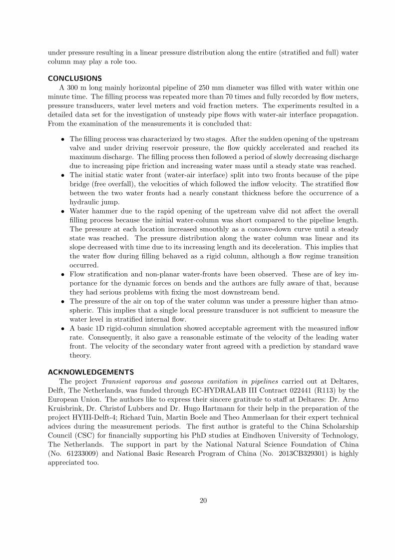
CONCLUSIONSA 300 m long mainly horizontal pipeline of 250 mm diameter was filled with water within one

minute time. The filling process was repeated more than 70 times and fully recorded by flow meters,pressure transducers, water level meters and void fraction meters. The experiments resulted in adetailed data set for the investigation of unsteady pipe flows with water-air interface propagation.From the examination of the measurements it is concluded that:

• The filling process was characterized by two stages. After the sudden opening of the upstreamvalve and under driving reservoir pressure, the flow quickly accelerated and reached itsmaximum discharge. The filling process then followed a period of slowly decreasing dischargedue to increasing pipe friction and increasing water mass until a steady state was reached.

• The initial static water front (water-air interface) split into two fronts because of the pipebridge (free overfall), the velocities of which followed the inflow velocity. The stratified flowbetween the two water fronts had a nearly constant thickness before the occurrence of ahydraulic jump.

• Water hammer due to the rapid opening of the upstream valve did not affect the overallfilling process because the initial water-column was short compared to the pipeline length.The pressure at each location increased smoothly as a concave-down curve until a steadystate was reached. The pressure distribution along the water column was linear and itsslope decreased with time due to its increasing length and its deceleration. This implies thatthe water flow during filling behaved as a rigid column, although a flow regime transitionoccurred.

• Flow stratification and non-planar water-fronts have been observed. These are of key im-portance for the dynamic forces on bends and the authors are fully aware of that, becausethey had serious problems with fixing the most downstream bend.

• The pressure of the air on top of the water column was under a pressure higher than atmo-spheric. This implies that a single local pressure transducer is not sufficient to measure thewater level in stratified internal flow.

• A basic 1D rigid-column simulation showed acceptable agreement with the measured inflowrate. Consequently, it also gave a reasonable estimate of the velocity of the leading waterfront. The velocity of the secondary water front agreed with a prediction by standard wavetheory.

ACKNOWLEDGEMENTSThe project Transient vaporous and gaseous cavitation in pipelines carried out at Deltares,

Delft, The Netherlands, was funded through EC-HYDRALAB III Contract 022441 (R113) by theEuropean Union. The authors like to express their sincere gratitude to staff at Deltares: Dr. ArnoKruisbrink, Dr. Christof Lubbers and Dr. Hugo Hartmann for their help in the preparation of theproject HYIII-Delft-4; Richard Tuin, Martin Boele and Theo Ammerlaan for their expert technicaladvices during the measurement periods. The first author is grateful to the China ScholarshipCouncil (CSC) for financially supporting his PhD studies at Eindhoven University of Technology,The Netherlands. The support in part by the National Natural Science Foundation of China(No. 61233009) and National Basic Research Program of China (No. 2013CB329301) is highlyappreciated too.

20

APPENDIX I. REFERENCES

Arai, K. and Yamamoto, K. (2003). “Transient analysis of mixed free-surface-pressurized flowswith modified slot model (Part1: Computational model and experiment).” Proc. 4th ASME-JSME Joint Fluids Summer Engineering Conf., Honolulu, Hawaii, USA, FEDSM2003–45266,2907–2913. ASME, New York.

Axworthy, D. H. and Karney, B. W. (1997). “Discussion of ‘Filling of pipelines with undulatingelevation profiles,’ by Liou, C. P. and Hunt, W. A..” J. Hydraul. Engrg., ASCE, 123(12), 1170–1174.

Bergant, A., Hou, Q., Keramat, A., and Tijsseling, A. S. (2011). “Experimental and numericalanalysis of water hammer in a large-scale PVC pipeline apparatus.” Proc., 4-th Int. Meetingon Cavitation and Dynamic Problems in Hydraulic Machinery and Systems, IAHR, Belgrade,Serbia, 27–36.

Bergant, A., van ’t Westende J. M. C., Koppel, T., Gale, J., Hou, Q., Pandula, Z., and Tijsseling,A. S. (2010). “Water hammer and column separation due to accidental simultaneous closureof control valves in a large scale two-phase flow experimental test rig.” Proc., Pressure Vessels& Piping Division / K-PVP Confrence, ASME, Bellevue, Washington, USA, Paper PVP2010–26131, Vol. 3, 923–932.

Cabrera, E., Abreu, J., Perez, R., and Vela, A. (1992). “Influence of liquid length variation inhydraulic transients.” J. Hydraul. Engrg., 118(12), 1639–1650.

Cabrera, E., Izquierdo, J., Abreu, J., and Iglesias, P. L. (1997). “Discussion of ‘Filling of pipelineswith undulating elevation profiles,’ by Liou, C. P. and Hunt, W. A..” J. Hydraul. Engrg., ASCE,123(12), 1170–1174.

De Martino, G., Fontana, N., and Giugni, M. (2008). “Transient flow caused by air expulsionthrough an orifice.” J. Hydraul. Engrg., ASCE, 134(9), 1395–1399.

Guizani, M., Vasconcelos, J. G., Wright, S. J., and Maalel, K. (2006). “Investigation of rapid fillingin empty pipes.” Intelligent Modeling of Urban Water Systems, Monograph 14, James, Irvine,McBean, and Pitt, eds., Computational Hydraulics International Ed.

Guo, Q. and Song, C. S. S. (1990). “Surging in urban storm drainage systems.” J. Hydraul. Engrg.,ASCE, 116(12), 1523–1537.

Hamam, M. A. and McCorquidale, J. A. (1981). “Transition of gravity to surcharge flow in sewers.”Int. Symp. on Urban Hydrology, Hydraulics and Sediment Control, Lexington, USA, 173–177.

Hou, Q. (2012). “Simulating unsteady conduit flows with smoothed particle hydrodynamic-s.” PhD Thesis, Eindhoven Univ. of Tech., Eindhoven, The Netherlands. Available fromhttp://repository.tue.nl/733420.

Hou, Q., Tijsseling, A. S., Laanearu, J., Annus, I., Koppel, T., Bergant, A., Vuckovic, S., An-derson, A., van ’t Westende, J. M. C., Pandula, Z., and Ruprecht, A. (2012a). “Experimentalstudy of filling and emptying of a large-scale pipeline.” CASA Report, 12-15, ISSN 0926-4507,Dept.of Math. and Comput. Sci., Eindhoven Univ. of Tech., The Netherlands. Available fromhttp://www.win.tue.nl/analysis/reports/rana12-15.pdf.

Hou, Q., Zhang, L. X., Tijsseling, A. S., and Kruisbrink, A. C. H. (2012b). “Rapid filling of pipelineswith the SPH particle method.” Procedia Engineering, 31, 38–43.

Izquierdo, J., Fuertes, V. S., Cabrera, E., Iglesias, P. L., and Carcıa-Serra, J. (1999). “Pipelinestart-up with entrapped air.” J. Hydraul. Res., IAHR, 37(5), 579–590.

Keramat, A., Tijsseling, A. S., Hou, Q., and Ahmadi, A. (2012). “Fluid-structure interaction withpipe-wall viscoelasticity during water hammer.” J. Fluid. Struct., 28, 434–455.

Laanearu, J., Annus, I., Koppel, T., Bergant, A., Vuckovic, S., Hou, Q., Tijsseling, A. S., Anderson,A., and van ’t Westende, J. M. C. (2012). “Emptying of large-scale pipeline by pressurized air.”

21

J. Hydraul. Engrg., ASCE, 138(12), 1090–1100.Laanearu, J., Bergant, A., Annus, I., Koppel, T., and van ’t Westende, J. M. C. (2009). “Some

aspects of fluid elasticity related to filling and emptying of large-scale pipeline.” Proc., 3-rdInt. Meeting on Cavitation and Dynamic Problems in Hydraulic Machinery and Systems, IAHR,Brno, Czech Republic, 465–474.

Laanearu, J. and van ’t Westende, J. M. C. (2010). “Hydraulic characteristics of test rig used infilling and emptying experiments of large-scale pipeline.” Proc. Hydralab III Joint User Meeting,Hannover, Germany, 5C8.

Lee, N. H. (2005). “Effect of pressurization and expulsion of entrapped air in pipelines.” PhDThesis, Georgia Institute of Technology, Atlanta, USA.

Lee, N. H. and Martin, C. S. (1999). “Experimental and analytical investigation of entrappedair in a horizontal pipe.” Proc. 3rd ASME-JSME Joint Fluids Summer Engineering Conf., SanFrancisco, USA, FEDSM99–6881, 1–8. ASME, New York.

Liou, C. P. and Hunt, W. A. (1996). “Filling of pipelines with undulating elevation profiles.” J.Hydraul. Engrg., ASCE, 122(10), 534–539.

Liu, D. Y. and Suo, L. S. (2004). “Rigid model for transient flow in pressurized pipe systemcontaining trapped air mass.” Adv. Water Sci., 16(6), 717–721 (in Chinese).

Lubbers, C. L. (2007). “On gas pockets in wastewater pressure mains and their effect on hydraulicperformance.” PhD Thesis, Delft University of Technology, Delft, The Netherlands.

Malekpour, A. and Karney, B. W. (2008). “Rapidly filling analysis of pipelines using an elasticmodel.” Proc., 10-th International Conference on Pressure Surges, BHR Group, Edinburgh, UK,539–552.

Malekpour, A. and Karney, B. W. (2011). “Rapid filling analysis of pipelines with undulatingprofiles by the method of characteristics.” Applied Mathematics, ISRN, Article ID 930460.

Martin, C. S. (1976). “Entrapped air in pipelines.” Proc., 2nd Int. Conf. on Pressure Surges, BHRA,London, UK, 15–27.

Martin, C. S. and Lee, N. (2012). “Measurement and rigid column analysis of expulsion of entrappedair from a horizontal pipe with an exit orifice.” Proc., 11-th International Conference on PressureSurges, BHR Group, Lisbon, Portugal, 527–542.

Nydal, O. J. and Andreussi, P. (1991). “Gas entrainment in a long liquid slug advancing in a nearhorizontal pipe.” Int. J. Multiphase Flow, 17(2), 179–189.

Ocasio, J. A. (1976). “Pressure surging associated with pressurization of pipelines containing en-trapped air.” Special m. s. research rep., School of Civil Eng., Georgia Institute of Technology,Atlanta, USA.

Razak, T. and Karney, B. W. (2008). “Filling of branched pipelines with undulating elevationprofiles.” Proc., 10-th International Conference on Pressure Surges, BHR Group, Edinburgh,UK, 473–487.

Tijsseling, A. S. (1996). “Fluid-structure interaction in liquid-filled pipe systems: A review.” J.Fluid. Struct., 10(2), 109–146.

Trajkovic, B., Ivetic, M., Calomino, F., and D’Ippolito, A. (1999). “Investigation of transition fromfree surface to pressurized flow in a circular pipe.” Water Sci. Technol., 39(9), 105–112.

Trindade, B. C. and Vasconcelos, J. G. (2013). “Modeling of water pipeline filling events accountingfor air phase interactions.” J. Hydraul. Engrg., ASCE, 139(9), 921–934.

Vasconcelos, J. G. (2005). “Dynamic approach to the description of flow regime transition in s-tormwater systems.” PhD Thesis, Univ. of Michigan, Ann Arbor, USA.

Vasconcelos, J. G. and Wright, S. J. (2005). “Experimental investigation of surges in a stormwaterstorage tunnel.” J. Hydraul. Engrg., ASCE, 131(10), 853–861.

Vasconcelos, J. G., Wright, S. J., and Guizani, M. (2005). “Experimental investigations on rapid

22

filling of empty pipelines.” Report UMCEE-05-01, Dept. of Civil Environ. Engrg., Univ. of Michi-gan, Ann Arbor, USA.

Wiggert, D. C. (1972). “Transient flow in free-surface, pressurized systems.” J. Hydraul. Div.,ASCE, 98(1), 11–27.

Wiggert, D. C. and Tijsseling, A. S. (2001). “Fluid transients and fluid-structure interaction inflexible liquid-filled piping.” Appl. Mech. Rev., 56, 455–481.

Yamamoto, K., Arai, K., and Asamizu, T. (2000). “Transient analysis for mixed free-surface-pressure flows: Estimation of entrapped air by lumped parameter model.” Turbomechanery,28(6), 364–371 (in Japanese).

Zhou, F. (2000). “Effects of trapped air on flow transients in rapidly filling sewers.” PhD Thesis,Univ. of Alberta, Alberta, Canada.

Zhou, F., Hicks, F. E., and Steffler, P. M. (2002). “Observations of air-water interaction in a rapidlyfilling horizontal pipe.” J. Hydraul. Engrg., ASCE, 128(6), 635–639.

Zhou, L., Liu, D. Y., and Karney, B. (2013a). “Investigation of hydraulic transients of two entrappedair pockets in a water pipeline.” J. Hydraul. Engrg., ASCE, 139(9), 949–959.

Zhou, L., Liu, D. Y., Karney, B., and Wang, P. (2013b). “The phenomenon of white mist in waterrapidly filling pipeline with entrapped air pocket.” J. Hydraul. Engrg., ASCE, In press.

Zhou, L., Liu, D. Y., Karney, B., and Zhang, Q. (2011). “Influence of entrapped air pockets onhydraulic transients in water pipelines.” J. Hydraul. Engrg., ASCE, 137(12), 1686–1692.

23

APPENDIX II. SPEED OF PROPAGATION OF DISTURBANCES IN CIRCULAR CHANNELFLOW

The filling process is characterised by a leading water front propagating at speed V1 and asecondary front propagating at speed V2, as sketched in Fig. 6c. Alternatively, one can regard thesecondary front as a disturbance propagating on top of the leading water column. The disturbancetravels at speed V1 − V2 in upstream direction. The theoretical speed of propagation is (Wiggert1972):

c =

√

gWt

A(1)

where A and Wt are the area and top width of the prismatic flow section, respectively, and g = 9.81m/s2 is the gravitational acceleration. For a circular channel

A(ξ) =1

8πD2

[

1 +2

πarcsin (2ξ − 1) +

4

π(2ξ − 1)

√

ξ − ξ2]

(2)

andWt(ξ) = 2D

√

ξ − ξ2 (3)

where ξ = h/D is the ratio of water depth and pipe diameter. The dependence of propagationspeed c on dimensionless water-depth ξ for a pipe with an inner diameter of 0.235 m is shown inFig. 16a. For a water depth h = 0.192 m, the speed is c = 1.43 m/s, which compares very well withV1 − V2 = 1.45 m/s estimated from Tables 1 and 2. It is approximately the speed of propagationin a rectangular channel: cr =

√

g/h = 1.37 m/s. The dimensionless speed c/cr is displayed inFig. 16b, which gives the deviation of speed in a circular channel from that in a rectangular channel.For h/D < 0.769 the speed in a circular channel is lower, otherwise it is higher.

(a) (b)

0 0.2 0.4 0.6 0.8 10

1

2

3

4

5

h/D

c (m

/s)

0 0.2 0.4 0.6 0.8 10

1

2

3

h/D

c/cr

FIG. 16. Speed of propagation c as function of water depth h: (a) dimensional for D = 0.235m; (b) dimensionless (independent of D).

Formula (1) has been derived for stationary flow with hydrostatic pressures. Both conditionsare violated in the experiments described herein.

24

APPENDIX III. RIGID-COLUMN MODELBased on the developments by Liou and Hunt (1996) and Axworthy and Karney (1997), a 1D

mathematical model has been established and implemented. Four assumptions state that the pipecross-section remains full during filling, that the pressure at the front is atmospheric, that thewater-pipe system is incompressible (i.e. rigid water column) and that the friction is quasi-steady.Define Hi as the head at the downstream end of pipe i. Suppose that the water front is travellingin the (i+ 1)-th pipe as shown in Fig. 17.

FIG. 17. Sketch of the filling of a pipeline with undulating elevation profile.

Applying Newton’s law of motion to the advancing water column in the (i+ 1)-th pipe yields

l(t)

gAi+1

dQ

dt= Hi −

fi+1l(t)

Di+1

Q2

2gA2i+1

+ l(t) sin θi+1, (4)

where l(t) is the length of the water column in the partially filled pipe, θ is the angle downwardfrom the horizontal, f is the Darcy-Weisbach friction factor, A = πD2/4 is the pipe cross-sectionalarea and Q = V A is the uniform flow rate. Similarly, for the fully-filled upstream pipes, we have

Lj

gAj

dQ

dt= Hj−1 −Hj −

fjLj

Dj

Q2

2gA2j

+ Lj sin θj , j = 2, · · · , i. (5)

Note that i depends on t. Due to entrance head loss and velocity head at the inlet, the equationfor the first pipe is slightly different and reads

L1

gA1

dQ

dt= HR −H1 −

(

K + 1 +f1L1

D1

)

Q2

2gA21

+ L1 sin θ1, (6)

where HR is the reservoir head and K the entrance loss coefficient. By adding the Eqs. (4), (5) and(6), all interior heads Hj (j = 1, · · · , i) are cancelled, and one equation is obtained for the fillingdischarge Q:

1

g

i∑

j=1

Lj

Aj

+l(t)

Ai+1

dQ

dt= HR −

i∑

j=1

fjLj

DjA2j

+fi+1l(t)

Di+1A2i+1

+K + 1

A21

Q2

2g

+

i∑

j=1

Lj sin θj + l(t) sin θi+1. (7)

25

Substituting the total length of the water column L(t),

L(t) =i

∑

j=1

Lj + l(t), (8)

into (7) gives

1

g(C1L(t) + C2)

dQ

dt= HR − (C3L(t) + C4 + C7)

Q2

2g+ C5L(t) + C6, (9)

where the time dependent (because of i) coefficients Ck (k = 1, · · · , 7) are defined as

C1 =1

Ai+1

, C2 =

i∑

j=1

Lj

Aj

− C1

i∑

j=1

Lj , C3 =fi+1

Di+1A2i+1

, C4 =

i∑

j=1

fjLj

DjA2j

− C3

i∑

j=1

Lj,

C5 = sin θi+1, C6 =

i∑

j=1

Lj sin θj − C5

i∑

j=1

Lj , C7 =K + 1

A21

.

The total water column length is related to flow rate Q by

L = L0 +

∫ t

0

Q

Ai+1

dt, (10)

where L0 (< L1) is the initial column length at t = 0 in pipe 1. In Eqs. (9) and (10), i is the indexof the latest pipe that has been fully filled. It starts from 0, indicating that pipe one is partiallyfilled. When L(t) becomes larger than L1, i becomes 1. When L(t) becomes larger than L1 + L2,i becomes to 2, and so on.

Now we have two coupled equations, (9) and (10), for the two unknowns Q and L. Equation(9) is an ODE with the initial condition

Q(0) = 0. (11)

Equation (10) is an integral equation in which Ai+1 depends on time. ODE (9) is integrated withthe fourth-order Runge-Kutta method and Eq. (10) with Simpson’s rule.

26

APPENDIX IV. NOTATIONThe following symbols and abbreviations are used in this paper:

A = cross-sectional area [m2]c = wave propagation speed [m/s]

Ci = i -th coefficient in Eq. (9)D = pipe inner diameter [m]e = pipe wall thickness [m]f = Darcy-Weisbach friction factor [-]g = gravitational acceleration [m/s2]h = water depth [m]hf = friction head loss [m]hlb = local head loss due to long bend [m]H = head [m]

HR = reservoir head [m]i, j = indexK = head loss coefficient [-]

l, L = length [m]p = pressure [barg]R = elbow radius of curvature [m]V = velocity [m/s]W = width [m]

x, y, z = coordinate [m]ρ = mass density [kg/m3]θ = angle [o]ξ = dimensionless depth [-]∀ = volume [m3]

FSI = fluid-structure interactionMOC = method of characteristicsODE = ordinary differential equationPDE = partial differential equationPVC = polyvinyl chlorideSPH = smoothed particle hydrodynamics

T = temperatureVF = void fractionVi = i-th valve

WL = water level

27

PREVIOUS PUBLICATIONS IN THIS SERIES:

Number Author(s) Title Month

13-31 13-32 13-33 13-34 13-35

R. Pulch E.J.W. ter Maten K. Kumar M. Neuss-Radu I.S. Pop Q. Hou A.C.H. Kruisbrink F.R. Pearce A.S. Tijsseling T. Yue Q. Hou A.S. Tijsseling Z. Bozkus Q. Hou A.S. Tijsseling J. Laanearu I. Annus T. Koppel A. Bergant S. Vučkovič A. Anderson J.M.C. van ‘t Westende

Stochastic Galerkin methods and model order reduction for linear dynamical systems Homogenization of a pore scale model for precipitation and dissolution in porous media Smoothed particle hydrodynamics simulations of flow separation at bends Dynamic force on an elbow caused by a traveling liquid slug Experimental investigation on rapid filling of a large-scale pipeline

Nov. ‘13 Dec. ‘13 Dec. ‘13 Dec. ‘13 Dec. ‘13

Ontwerp: de Tantes,

Tobias Baanders, CWI