13, allée François Mitterrand BP 13633 49100 ANGERS Cedex 01 Tél. : +33 (0) 2 41 96 21 06

Web : http://www.univ-angers.fr/granem

Pawel Ciompa and the meaning of

econometrics: A comparison of two

concepts

Karl-Friedrich Israel GRANEM, Université d’Angers

septembre 2016

Document de travail du GRANEM n° 2016-06-052

Pawel Ciompa and the meaning of econometrics: A comparison of two concepts Karl-Friedrich Israel Document de travail du GRANEM n° 2016-06-052 septembre 2016 Classification JEL : B23, B31, B53, C10 Mots-clés : économétrie, Pawel Ciompa, Ragnar Frisch, économie autrichienne. Keywords: econometrics, Pawel Ciompa, Ragnar Frisch, Austrian economics.

Résumé : Une comparaison entre la conception de l'économétrie par Pawel Ciompa et la conception moderne selon Ragnar Frisch et les autres membres de la Société d’économétrie est présentée dans cet article. Ciompa est le premier économiste à avoir utilisé et défini le terme allemand « Oekonometrie » en 1910, seize ans avant Frisch, qui a introduit le terme équivalent « économétrie » en français. Ciompa concevait l'économétrie comme entièrement descriptive, comme un ensemble d'outils dédiés à la transmission d'informations dans le domaine de la comptabilité. Frisch, en revanche, considérait l'économétrie comme une approche quantitative à la théorie économique, c’est-à-dire comme l’unification de la théorie économique avec les méthodes statistiques et mathématiques. Une justification de l'usage de cette dernière conception requiert des considérations d'ordre méthodologiques et épistémologiques, alors que l’application de la conception de Ciompa est seulement une question de style et d'exposition. Il manque cependant une justification satisfaisante pour l'usage de la conception de l'économétrie moderne, notamment à la lumière des critiques émises par les économistes dits Autrichiens. Leur argument principal, qui avance que le principe de constance n’est pas satisfait en économie, est illustré ici par une simulation informatique. J'en conclus que l’économétrie moderne devrait renouer avec sa nature descriptive telle que Ciompa lui avait attachée au départ. Abstract: Pawel Ciompa’s conception of econometrics is compared with the modern mainstream interpretation of the term that originated with Ragnar Frisch and other members of the Econometric Society. Ciompa was the first to use the German language term “Oekonometrie” in 1910, sixteen years prior to Frisch, who used the French equivalent “économétrie”. Ciompa conceived of econometrics as being entirely descriptive. He considered it to be a set of tools for facilitating the conveyance of information in the field of accounting. In contrast, Frisch regarded it as a quantitative approach to economic theorizing, i.e. as the unification of economic theory, mathematics and statistics. A justification for applying the latter conception of econometrics requires methodological and epistemological considerations, whereas applying the former conception is merely a matter of style. However, a satisfactory justification for applying econometrics in the commonly accepted sense is lacking, and strong arguments against it have been brought forward among others by economists of the Austrian School. The argument that the constancy principle is not satisfied in the field of economics is illustrated by means of a computer simulation. I conclude that modern econometrics should be pushed back towards the descriptive character that Pawel Ciompa originally attached to the term.

Karl-Friedrich Israel Faculté de Droit, Economie et Gestion Université d’Angers kf_israel@gmx.de

© 2016 by Karl-Friedrich Israel. All rights reserved. Short sections of text, not to exceed two paragraphs, may be quoted

without explicit permission provided that full credit, including © notice, is given to the source. © 2016 par Karl-Friedrich Israel. Tous droits réservés. De courtes parties du texte, n’excédant pas deux paragraphes, peuvent être citées sans la permission des auteurs, à condition que la source soit citée.

1

Pawel Ciompa and the meaning of econometrics: A comparison of two concepts

Karl-Friedrich Israel

Introduction

Pawel Ciompa’s conception of econometrics seems to be long forgotten, if it has ever exerted any

noteworthy effect on the broader discipline of economics at all. There is no entry on Ciompa in

any of the major English, French or German language encyclopedias. There is only a very short

entry in the first volume of the third edition of the Polish Wielka Encyklopedia Powszechna

PWN from 1983 (Wiśniewski 2016, p. IX). Yet, in the more recent editions of its successor, the

Wielka Encyklopedia PWN, the entry on Pawel Ciompa has been removed.1 It is true, his name is

sometimes mentioned when it comes to the origins of the term “econometrics”, but usually not

more than the equivalent of a brief footnote is devoted to his work. Not even Ragnar Frisch, the

originator of econometrics in the modern sense (Bjerkholt 1995), who famously defined the “new

discipline” in 1926, was initially aware of Ciompa’s work and his use of the same term for

something rather distinct some sixteen years earlier. Frisch has admitted this in a brief note in his

journal Econometrica (Frisch 1936).

It was professor Tomasz Lulek of the university of Cracow, who informed the editor of

Econometrica about the fact that the term econometrics has already been used and defined by

Ciompa in 1910 as the “geometrical representation of value”,2 which was considered to be closely

related to the principles of accounting. It is interesting to note that Frisch (1936, p. 95) laments:

It still seems, however, that, taken in the now accepted meaning, namely, as the unification of

economic theory, statistics, and mathematics, the word was first employed in the 1926 paper

1 I thank Dr. Łukasz Dominiak from Nicolaus Copernicus University in Toruń, Poland, for his assistance in this

enquiry.

2 In the German original: „die geometrische Darstellung des Wertes.“ (Ciompa 1910, p. 5) We will go into much more detail in the second section of this paper.

2

[(Frisch 1926b)]. Pawel Ciompa seems to emphasise too much the descriptive side of what is

now called econometrics.

In the above quote, Frisch in effect points to the fundamental difference between the two

conceptions of econometrics, which shall constitute a central concern of this paper. Should we

think about econometrics as being merely descriptive, as Ciompa did, or can we reasonably attach

more to its meaning and scope, following Frisch and the majority of modern economists?

First of all, Ciompa’s vision of econometrics is presented in the next section of this paper,

followed by a discussion of Frisch’s conception of the term, which essentially represents the

modern mainstream view. Thereafter, a central point of criticism against the modern

interpretation of econometrics from the point of view of Austrian economics is discussed and

illustrated by means of a computer simulation. The lack of constancy in economics that the

Austrians stress, suggests a return to a more Ciompanian view. It is however important to make

clear from the outset that I do not subscribe to Ciompa’s theory in all its details. The point I wish

to emphasize and support is that Ciompa thought of economic theory as being prior to, and

more fundamental than, econometrics, which is based on economic theory, but does not provide

the means to alter it. The paper ends with some concluding remarks.

Pawel Ciompa’s Conception of “Oekonometrie”

Polish economist Pawel Ciompa (1867-1913) was a professor at the Higher School of Economics

in Cracow and director of accounting at the federal state bank of Galicia based in Lemberg. The

full name of his home region was Kingdom of Galicia and Lodomeria and the Grand Duchy of Cracow

with the Duchies of Auschwitz and Zator. It was also known as the Halychyna or Austrian Poland and

was part of the dual-monarchic Austro-Hungarian Empire at that time. Hence, “ruler of Galicia

and Lodomeria” was part of the ceremonial titles of the princes of Hungary. Today the region

belongs partly to Poland and partly to the Ukraine. Its former capital Lemberg is today called

Lviv and part of western Ukraine, whereas Cracow lies in Southern Poland.

3

Ciompa published his German language book Grundrisse einer Oekonometrie und die auf der

Nationaloekonomie aufgebaute natürliche Theorie der Buchhaltung (Outline of econometrics and the natural theory

of accounting based on economics, from now on simply referred to as Grundrisse) in 1910, in which he

defended an economic, as opposed to a juridical, approach to the theory of accounting

(Mattessich 2008, p. 270). In the Grundrisse, one finds the earliest mention and definition of the

term econometrics, more precisely, its German language equivalent “Oekonometrie” (also

“Ökonometrie”), as far as we know. Ciompa describes the new term vividly:

Just like mechanical, acoustical, dynamic, and other such phenomena in physics, and mass

phenomena in geometry, also economic phenomena should be represented and displayed

following a doctrine, which I envision as a sort of economographics. This economographics would

constitute a descriptive economics; it would have to be based on economics, mathematics and

geometry. The foremost task of such a doctrine would be the geometrical representation of

value. This part of economographics I call econometrics. The practical application of

econometrics to the mathematical representation of values and their changes would be

accounting. Put differently, econometrics would then just be the theory of accounting.

[emphasis added]3

Econometrics in Ciompa’s vision, and what it adds to the more general field of economics, would

therefore be strictly descriptive in nature. Its purpose is to describe and depict the changes and

evolution of economic values. More specifically, he thought of it as being a collection of

mathematical and graphical tools by which we could describe and depict the evolution of assets

and liabilities in business accounting. He further explains the scientific status of economographics

and econometrics as follows:

3 All quoted passages from the Grundriss in this paper have been translated by myself. In the German original (Ciompa 1910, p. 5) we read:

Wie die mechanischen, akustischen, dynamischen und dgl. Erscheinungen durch die Physik oder wie die Massenerscheinungen durch die Geometrie, so sollten auch die volkswirtschaftlichen Erscheinungen durch eine Lehre, die ich mir als eine Art Oekonomographie vorstelle, zur Darstellung gebracht werden. Diese Oekonomographie waere eine Art darstellende Nationaloekonomie, sie muesste auf der Nationaloekonomie, Mathematik und Goemetrie aufgebaut werden. Einer solchen Lehre wuerde dann vor allem die geometrische Darstellung des Wertes zufallen. Diesen Teil der Oekonomographie nenne ich Oekonometrie. Die praktische Anwendung dieser Oekonometrie auf die mathematische Darstellung der Werte und deren Veraenderungen ist dann die Buchhaltung. Umgekehrt ist dann die Oekonometrie nur die Theorie der Buchhaltung.

In the remainder of the paper, the original German quotations only are provided, when my English translations are running the risk of becoming too inaccurate for a proper understanding of what Ciompa actually wrote.

4

Similar to trigonometry which is a subfield of geometry, econometrics would be a subfield of

economographics. Accounting and econometrics would be related to each other just like

mathematics and algebra. (pp. 5-6)

This latter comparison is very thought-provoking. Algebra, in its broadest sense, combines

elements from almost all of mathematics. It provides us with the rules of how to manipulate

mathematical symbols and formulas in general, and so it enters into almost any other subfield of

mathematics. It contains the basic armamentarium that any layperson interested in mathematics,

and a fortiori, any professional mathematician, needs in order to communicate mathematical

results to an audience. In this sense, algebra might be understood as containing the tools of

communication for mathematical insights and knowledge. In very much the same way, it seems,

Ciompa considered econometrics to be the apparatus which we should use in order to

communicate and illustrate information in accounting.

In order to clarify the subject matter of business accounting, and hence of econometrics, Ciompa

starts the Grundrisse with a brief discussion of economic value theory and the theory of goods.

Although he is a bit imprecise in his exposition, we find several classical definitions and well-

known classifications of economic concepts: a good is simply defined as any means, material or

immaterial, that is conducive to the satisfaction of human wants. Goods are classified into

economic goods that have an exchange value, free goods that have no exchange value, and services,

which are defined as any outflow of human activity that has an exchange value (Ciompa 1910, pp.

1-2).4 Ciompa points out, that only economic goods, which according to his own definitions

subsume services, are relevant for business accounting.

4 Obviously, according to this classification, services are just a subgroup of economic goods. Technically speaking,

the classification is therefore not a partition. It is not clear why Ciompa mentions services at all on this level of his classification scheme, but this should not disturb us too much. In the remainder of the book, he is almost always only referring to economic goods, which includes services.

5

Next, Ciompa makes the twofold distinction of value into use value and exchange value, both of

which can be either of subjective or objective nature.5 From these distinctions he obtains the terms

subjective use value that is assigned to a good in accordance with the subjective importance of the

wants that it satisfies, subjective exchange value, which is assigned to a good in accordance with the

importance of the wants that can be satisfied by those goods that can be obtained in exchange for

it, objective use value that describes the factual or natural scientific potential of a good to satisfy

wants, and objective exchange value, which is simply the market value or the price of the good as the

result of the subjective evaluations of buyers and sellers. Ciompa further points out, that value is

not inherent in the good, but contingent on needs, inclinations, the economic situation of the

individual, and also the social environment. It is therefore subject to constant change, and the

only way to reliably gain information about the value of a good is through exchange. It is then the

objective exchange value with which accounting is primarily concerned (p. 4).

What Ciompa defines as the normal value [Normalwert] of a good or service corresponds to its

cost of production. A rent or a profit is earned whenever the realized objective exchange value

on the market exceeds the normal value. A loss is incurred whenever the realized objective

exchange value is below the normal value of the good.

In order to be able to uniformly quantify and express objective exchange values, profits and

losses, Ciompa has emphasized the importance of money and money prices. He simply defines

money as just another good, and prices as proportions of values, and here surely means objective

exchange values.6 He writes:

5 This classification scheme is known for example from Ciompa’s fellow countryman Carl Menger (2007 [1871], pp.

121ff. and 226ff.), but at least the distinction between use and exchange value has a much longer tradition in the history of economic thought, for example over Pufendorf (1744) to the scholastic doctors of the Middle Ages, all the way back to the old Greeks (Rothbard 2006 [1995], ch. 1; Schumpeter 2006 [1954], part II, ch. 2). 6 This is another example of an imprecision in Ciompa’s exposition. Although, he made the above mentioned

distinctions into different kinds of values, he is in the remainder of his book usually only writing about “the value” as if there was only one. These inaccuracies notwithstanding, here again, we might argue that Ciompa follows his countrymen C. Menger and E. von Böhm-Bawerk, although he is not referencing to them and their work directly. Böhm stated that “organized exchange gives almost every good a second value” (Böhm-Bawerk 1930 [1891], p.

6

This proportion of values between two goods we call price. The price, therefore, is nothing

other than the expression of the value of one good in terms of the value of another; usually the

price is expressed in money. The value of money is not stable, but changes, as does the value

of any other good, because money itself is a good. (p. 9)

The next fundamental distinction that Ciompa makes is between wealth [Vermögen] and capital

[Kapital]. Wealth is understood as the set of all economic goods that one freely disposes of (p. 9).

Wealth turns into capital if it is put to some productive use. Therefore, capital is understood as

productive wealth, or as the resultant of the “combination of wealth and labor” (p. 10).7 It is then

clear that we might also think about capital as being a subset of wealth. There can be no capital

without wealth, but there can be wealth without capital.8 Wealth is, in fact, “the basis for all

economic life” (pp. 9-10).

Economic life in Ciompa’s vision is composed of economic actions [wirtschaftliche Handlungen],

all of which are directed towards the use of some economic goods, or some capital, in order to

consume or create new wealth and capital. He is now able to pin down the proper function of

accounting and econometrics as follows:

The task of accounting is to mathematically calculate, and econometrically illustrate the yields

from wealth and capital as results of economic life. Economic life consists of processes and

actions, which use up old wealth v1 in order to create new wealth v2. As a result, the initial

wealth V1 diminishes, and it remains a wealth of V2=V1-v1, which then increases to the wealth

V3=V2+v2. The same holds true for the capital of this wealth; in the first instance, it

simultaneously diminishes C2=C1-c1; in the second instance, it simultaneously increases with the

wealth: C3=C2+c2.9

xxxiii), which is of course the exchange value, and then bluntly emphasized the indissoluble connection between price and exchange: “The law of Price, in fact, contains the law of Exchange Value.” (p. 132) Furthermore, Menger (2007 [1871], p. 257) has presented an account of the emergence of money as just another good with certain properties from the original state of barter exchange. 7 The careful reader realizes that at least a person’s own labor according to the proposed definitions must be seen as

a part of wealth, as it falls under the definition of services and therefore is an economic good. 8 It is clear that in practice, and from a broader perspective, it might be very difficult to decide what a productive use

of wealth is – an argument which has been brought forward against the idle resources argument for macroeconomic policy interventions during crises and recessions. However, for Ciompa’s purposes, it seems, the concepts are sufficiently well defined, as we could relatively easily find out which economic goods are used, and therefore constitute capital, in any specific and well-defined economic action, for example, the production of a wooden chair. 9 In the German original, we read:

7

In Ciompa’s view, economic life can be broken down into individual economic actions like the

one schematically described in the above quotation. In order to provide an impression of his

econometrics, a brief presentation of what he called the econometric Quadrigon, as well as the wealth

and capital accounts that emerge out of it, seems advisable. We take the numeric example that

Ciompa uses himself: V1=-C1=6, v1=-c1=3, v2=-c2=4 measured in money units K [Krone]. 10

Notice, Ciompa considered capital to be a negative quantity, hence the minus sign in the

equations, which is intuitively plausible, because capital is the part of the wealth that is put to

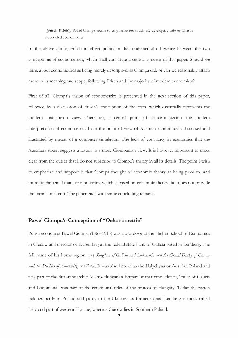
productive use, and hence, is used up in the production processes. We assume an initial wealth

endowment of V1=K6, which corresponds to a potential capital of -C1=K6, from which v1=-

c1=K3 is used up in a hypothetical economic action. Figure 1 illustrates the situation so far.

The econometric Quadrigon is always symmetric, as we know it from balance sheets in modern

accounting. Its upper left side captures the initial wealth of V1=K6, and the upper right side

corresponds to the potential capital -C1=K6. Both are illustrated as six equally shaped rectangles.

Again, to emphasize the conceptual difference between wealth and capital, different hatchings

have been chosen by the author of the Grundrisse. In the first step of the hypothetical economic

action, a part of the initial wealth, -v1=-K3, is used up as capital, c1=-K3, which is shown in the

bottom right quadrant and the bottom left quadrant, respectively. We have thus made 270° of the

full circle from upper left, over the upper right, the bottom right, to the bottom left of the

Quadrigon, and in each step switched between the concepts of wealth and capital. To complete

the circle, the second part of the hypothetical economic action must be considered. We assume

Die Buchhaltung hat die Aufgabe, die aus dem wirtschaftlichen Leben resultierenden Erfolge des Vermögens und Kapitals mathematisch resp. ökonometrisch zu berechnen resp. darzustellen. Das wirtschaftliche Leben besteht aus Prozessen und Handlungen, welche altes Vermögen v1 verbrauchen, um neues Vermögen v2 zu schaffen. Dadurch nimmt das ursprüngliche Vermögen V1 ab, es bleibt ein Vermögen V2=V1-v1, welches wiederum zum Vermögen V3=V2+v2 anwächst. Dasselbe geschieht mit dem Kapital dieses Vermögens; im ersten Falle nimmt es gleichzeitig ab und es verbleibt C2=C1-c1, im zweiten Falle nimmt es mit dem Vermögen gleichzeitig zu: C3=C2+c2. (Ciompa 1910, p. 14)

10

The Krone became the official currency in the Austro-Hungarian Empire in 1892 when the gold standard was adopted. It replaced the Gulden, which was defined in terms of silver.

8

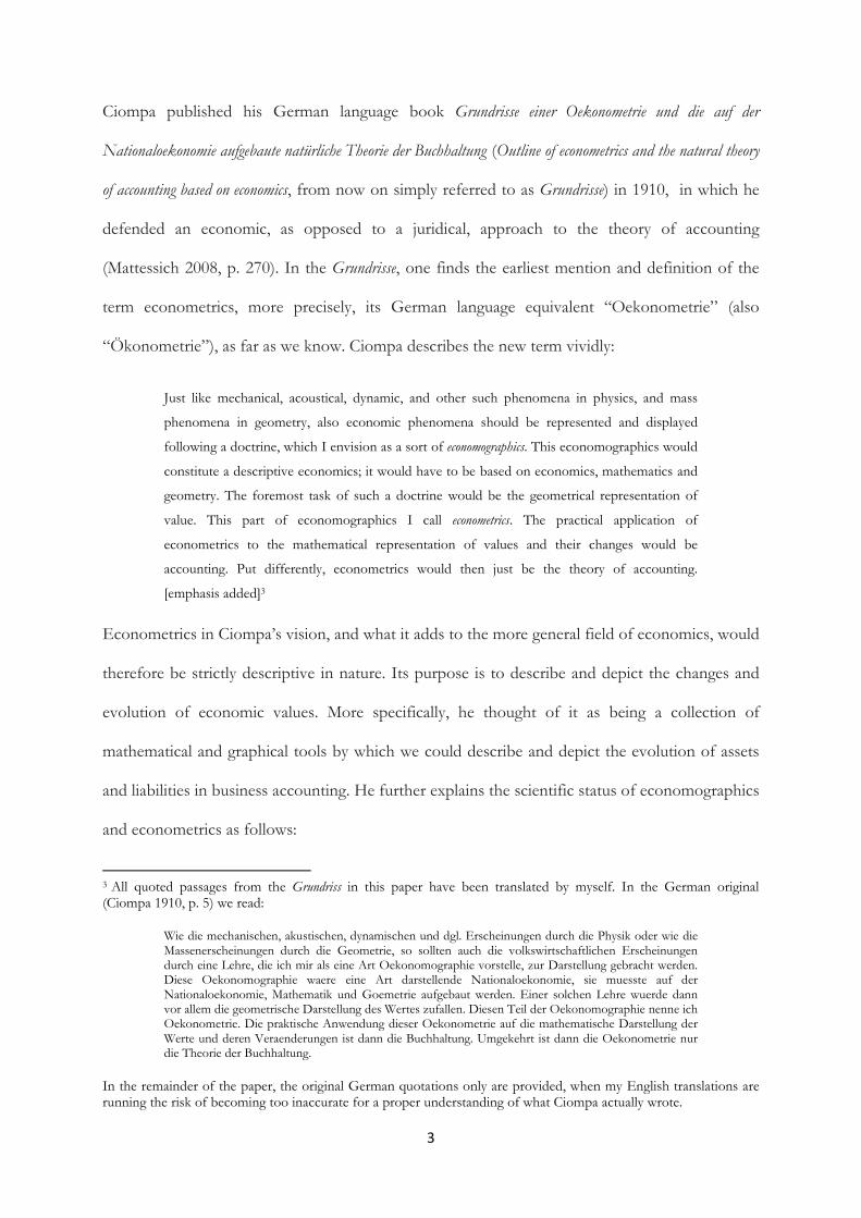
that the action yields new wealth of v2=K4, which corresponds to new potential capital of –

c2=K4. Figure 2 shows the complete econometric Quadrigon for this case.

The upper left side in Figure 2 also contains the new wealth, or what we might call the revenue of

the economic action, v2=K4. By symmetry, the new wealth corresponds to potential capital of -

c2=K4, as shown on the upper right side of the Quadrigon, which is now available for further

economic action.

Figure 1: Ciompa’s econometric Quadrigon from [Ciompa (1910, Fig. 16b, p. 15)]

Figure 2: Ciompa’s complete econometric Quadrigon [(Ciompa 1910, Fig. 17, p. 16)]

The complete economic action, including its cost, v1, its revenue, v2, as well as the corresponding

gain, v2-v1, can also be documented in rather mundane wealth and capital accounts, and it certainly

is subject to debate, whether this might not, after all, be the more sensible way of presenting “the

9

yields from wealth and capital”.11 As mentioned above, wealth is considered a positive value and

capital is negative. Hence, in the wealth account, we find initial wealth and revenue on the debit

side [Soll], and the costs and net total on the credit side of the account [Haben]. For the capital

account, we have the inverse arrangement.

Debit wealth account Credit

1) initial wealth V1=K6 2) cost v1=K3

3) revenue v2=K4 4) net total V3=K7

v2+V1= K10 v1+V3= K10

Debit capital account Credit

2) cost c1=K3 1) initial capital C1=K6

3) net total C3=K7 3) revenue c3=K4

C3+c1= K10 C1+c3= K10

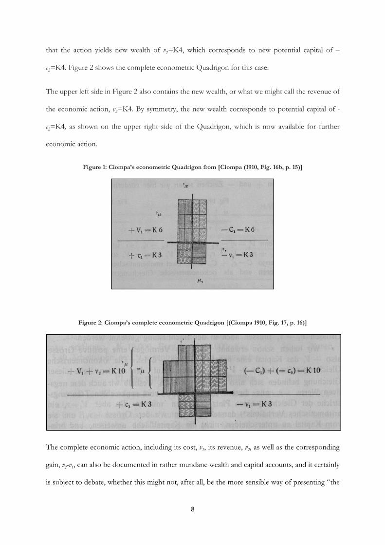
Figure 3: Econometric Quadrigon capturing multiple economic actions [(Ciompa 1910, Fig. 100, p. 95)]

This Quadrigon captures three instances of revenue generation, ´´´x=K6, ´´x=K4, ´x=K6, as well as three instances of cost expenditures, x,=K2, x,,=K6, x,,,=K4. The net total in this case corresponds to K4.

In the remainder of Part I [Oekonometrische primäre Gleichungen und oekonometrische Verhältnisse] and in

Part II [Oekonometrische sekundäre und tertiäre Gleichungen] of the Grundrisse, Ciompa elaborates on

11 The two tables correspond to Fig. 21 and Fig. 22 in Ciompa (1910, p. 17).

10

this basic example of an economic action. He adds a couple of complications, such as variations

in the per unit price of goods, or in the quantity of goods (like losses from inadequate storage),

and explains how these cases enter into his econometric accounting scheme. Ciompa also

presents an econometric Quadrigon that captures more than one economic action of selling and

buying certain quantities of a good. The graphical representation thereby becomes increasingly

complicated as illustrated in Figure 3.

Part III [Bewertung des Kapitalvermögens in der Bilanz] covers the balancing of accounts and some

criticism of accounting rules and practices in Austro-Hungary and Germany at that time. 12

Ciompa emphasizes again, that accounting and econometrics must be based on economic theory,

and in particular on the economic theory of value (p. 134).

As pointed out in the introduction of the paper, my purpose is neither to describe nor to defend

Ciompa’s work in every detail. I believe that there are many shortcomings and inaccuracies in his

exposition. However, without evaluating his doctrine in its specificities, the important point that

merits emphasis is that his conceptions of econometrics and economographics are entirely

descriptive. They are attempts to build upon economic theory, without transforming it. Thus, it

stands in sharp contrast to the modern conception of econometrics, which is discussed next.

Ragnar Frisch and the Modern Conception of Econometrics

The celebrated originator of the modern conception of econometrics is Norwegian economist

Ragnar Frisch (1895-1973), who was the first recipient of the Nobel Memorial Prize in

12 Ciompa notes that “the truth and clarity of our balances is sinking further into a muddy subsoil. Today, it takes considerable effort to rescue the theory of accounting from the clutter that surrounds it.” (p. 136) He argues that differences in accounting rules for different types of businesses (privileges for corporations) and different types of equity, such as operational capital [Betriebsgegenstände] and goods for sale [Veräusserungsgegenstände] are unjustifiable on economic grounds. Everything should be based on universal principles.

11

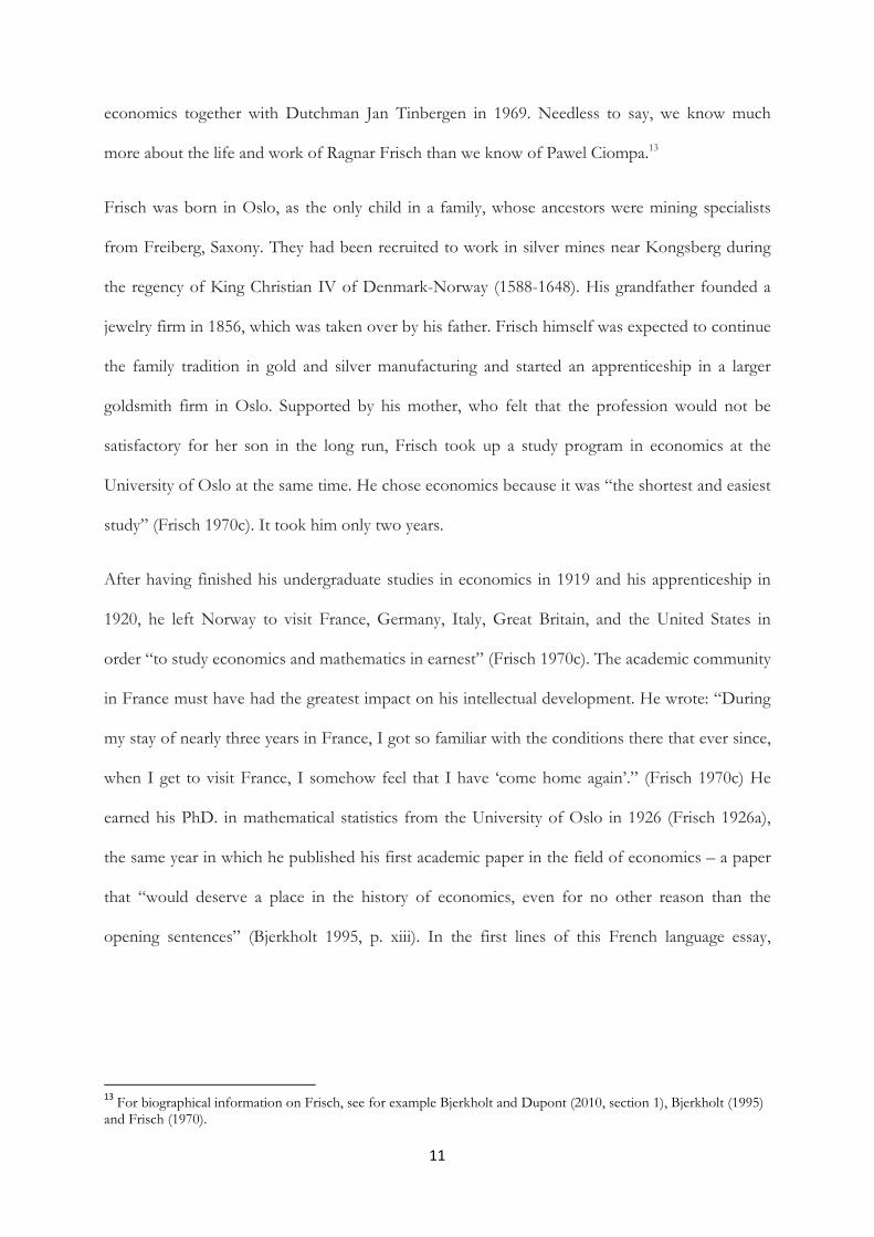
economics together with Dutchman Jan Tinbergen in 1969. Needless to say, we know much

more about the life and work of Ragnar Frisch than we know of Pawel Ciompa.13

Frisch was born in Oslo, as the only child in a family, whose ancestors were mining specialists

from Freiberg, Saxony. They had been recruited to work in silver mines near Kongsberg during

the regency of King Christian IV of Denmark-Norway (1588-1648). His grandfather founded a

jewelry firm in 1856, which was taken over by his father. Frisch himself was expected to continue

the family tradition in gold and silver manufacturing and started an apprenticeship in a larger

goldsmith firm in Oslo. Supported by his mother, who felt that the profession would not be

satisfactory for her son in the long run, Frisch took up a study program in economics at the

University of Oslo at the same time. He chose economics because it was “the shortest and easiest

study” (Frisch 1970c). It took him only two years.

After having finished his undergraduate studies in economics in 1919 and his apprenticeship in

1920, he left Norway to visit France, Germany, Italy, Great Britain, and the United States in

order “to study economics and mathematics in earnest” (Frisch 1970c). The academic community

in France must have had the greatest impact on his intellectual development. He wrote: “During

my stay of nearly three years in France, I got so familiar with the conditions there that ever since,

when I get to visit France, I somehow feel that I have ‘come home again’.” (Frisch 1970c) He

earned his PhD. in mathematical statistics from the University of Oslo in 1926 (Frisch 1926a),

the same year in which he published his first academic paper in the field of economics – a paper

that “would deserve a place in the history of economics, even for no other reason than the

opening sentences” (Bjerkholt 1995, p. xiii). In the first lines of this French language essay,

13

For biographical information on Frisch, see for example Bjerkholt and Dupont (2010, section 1), Bjerkholt (1995) and Frisch (1970).

12

published in a Norwegian periodical under the title “Sur un problème d’économie pure”,14 Frisch

famously defined the allegedly new discipline of “économétrie”:

Intermediate between mathematics, statistics, and political economy, we find a new discipline,

which, for lack of a better name, may be called econometrics.

It is the aim of econometrics to subject abstract laws of theoretical political economy or ‘pure’

economics to experimental and numerical verification, and thus to turn pure economics, as far

as possible, into a science in the strict sense of the word. [emphasis in the original]15

Thus, in stark contrast to Ciompa, Frisch did not only attempt to add a new layer to the existing

body of economic theory, but sought much more than that. He called for a genuine

transformation of economics into a “science in the strict sense.” The guiding ideal for his

scientific vision of econometrics is to be found in the natural sciences, and in particular in physics

and astronomy.16 In order to push this transformation further, Frisch has built upon, and was

inspired by, the ideas of several renowned economists, among which are Léon Walras (1834-

1910), William Sranley Jevons (1835-1882), Alfred Marshall (1842-1924), Vilfredo Pareto (1848-

1923), Knut Wicksell (1851-1926), Irving Fisher (1867-1947), and Joseph Schumpeter (1883-

14 An English translation of the article has been published in Chipman (1971, pp. 386-423) under the title “On a Problem in Pure Economics”. Having no access to the volume, quotations have been translated into English by myself. I follow the same policy of providing the French original only for passages that are of particular importance. All quotations come from the republication of the original French article in Metroeconomica in 1957. 15 In the French original, we read:

Intermédiaire entre les mathématiques, la statistique et l’économie politique, nous trouvons une discipline nouvelle que l’on peut, faute de mieux, désigner sous le nom de l’économétrie.

L’économétrie se pose le but de soumettre les lois abstraites de l’économie politique théorique ou l’économie ‘pure’ à une vérification expérimentale et numériques, et ainsi de constituer, autant que cela est possible, l’économie pure en une science dans le sens restreint de ce mot. (Frisch 1957 [1926b], p. 79)

16 After Irving Fisher had arranged a visiting professorship from his personal funds, Frisch came to Yale University in the early 1930s. In one of his lectures, he praised astronomy as being one of the most scientific fields, as “astronomical observations are filled into the theoretical structure […] Economic theory has not as yet reached the stage where its fundamental notions are derived from the technique of observations.” (Frisch 1930, ch. 1.1, as cited in Bjerkholt and Dupont 2010, p. 57) It would be false, however, to reduce Frisch’s ideal conception of econometrics to empiricism and little else, although, this is exactly what this particular statement suggests. In his lectures there are several other references to Newtonian physics and Einstein’s theory of general relativity.

13

1950).17 All of these economists were, to a greater or lesser extent, and if only occasionally, driven

by the attempt at formalizing and quantifying elements of economic theory, such as the concept

of utility. 18 Frisch himself considered the quantification of utility a primary objective of

econometrics:

The econometric study that we present is an attempt to realize Jevon’s dream [the author refers

to the paragraph Numerical Determination of the Laws of Utility in the fourth edition of Jevons

(1965 [1911], p. 146)]: measure the variations of the marginal utility of economic goods. We

consider in particular the variation of the marginal utility of money. (Frisch 1957 [1926], p. 79)

In his Nobel Memorial lecture, delivered after 44 years of an academic career as Norway’s leading

economist, professor and director of the Institute of Economics at the University of Oslo, co-

founder of the Econometric Society and editor of its journal Econometrica, he refers again to Jevon’s

dream of being “able to quantify at least some of the laws and regularities of economics”, and

claims that, “since the break-through of econometrics – this is not a dream anymore but a

reality.” (Frisch 1970a, p. 12) What then did the break-through look like? How did the dream

become true?

Frisch understood that the quantification of economic concepts and theory was a necessary

condition for the application of natural scientific methods to economics. These methods require

17

According to Bjerkholt (1995), Frisch’s two great mentors were Marshall and Wicksell (he refers to Frisch 1950, 1952). Apparently, their books were the only really worn-out ones in his personal library. Frisch credits Marshall for having combined the Walras-Jevons-Menger subjective notion of value with the cost of production viewpoint (Frisch 1970a, p. 16). He specifically refers to Menger as the head of the Austrian economists, but misspells his first name as Karl instead of Carl. Karl Menger (1902-1985), son of Carl Menger, was a mathematician and probably more after Frisch’s fancy. Obviously, Frisch was more drawn towards the formal mathematical presentation in Walras (1874) and Jevons (1965 [1871]), rather than the entirely verbal presentation in Menger (2007 [1871]). For an interesting de-homogenization of these three thinkers, see Jaffé (1976). Frisch studied a French translation of Fisher’s dissertation thesis Mathematical Investigations in the Theory of Value and Prices during his time in Paris (Bjerkholt and Dupont 2010, p.28, fn. 10). Fisher himself refers to Jevons’ Theory of Political Economy as one of two books that had the biggest influence on him (Fisher 1892, p. 3). Although, Walras and his successor at the University of Lausanne, Pareto, both made important contributions to the mathematical formalization of economic theory in general, and value theory in particular, it is important to note that Pareto rejected a cardinal interpretation of value and utility, but thought of them as being ordinal, and, in fact, based his famous welfare economics on ordinal utility (Aspers 2001). In this respect, Frisch departed from Pareto. Indeed, listing these economists as intellectual influences is not to suggest that they all would have celebrated Frisch’s work in every respect. 18

Schumpeter may of course be seen as the exception. He was not actively involved in this endeavor in his own writings, but enthusiastically supported the efforts of his mathematically inclined colleagues. Schumpeter, together with Frisch and Fisher, was a founding member of the Econometric Society in 1930 and its president from 1940-1941.

14

observability and measurability, ideally on cardinal scales. Methods of experimental and numerical

verification (or falsification) could not simply be applied to classical economic theory, as the

underlying core concepts possess no independent existence in the observable external world, and

its conclusions only take the form of qualitative or even counterfactual laws.19

The first task, therefore, is to redefine economic concepts in terms of variables and indicators

that are at least in principle observable and measurable, which allows the derivation of

quantitative economic relationships. Frisch, in the spirit of neoclassical economics, based this

redefinition on a mathematical axiomatization of human behavior that has become so widespread

that every undergraduate student of economics today learns certain forms of it in microeconomic

classes under the headings of rational behavior, utility maximization and homo oeconomicus. This

axiomatization comprises, for example, the well known assumptions of determination, additivity and

transitivity of preferences.20 Utility or value is not described as an abstract psychic phenomenon,

which is ultimately taken as a given, not to be explained further, but rather as a well defined

mathematical function of a vector of consumer goods.

Hence, utility is just understood as a mapping from multidimensional bundles of consumer

goods, which are observable as they have some form of physical existence, to some cardinal scale

of measurement. The critical aspect, of course, is the determination of the mapping. In Frisch’s

view, the fact that the mapping is merely assumed into existence should not cause too much

concern. He was convinced that it was determinable, in principle, through choice questions

[expériences par interrogation] posed to the respective individuals (Bjerkholt and Dupont 2010,

pp. 39-45; Frisch 1957 [1926b], p. 81, 2013 [1933], Lecture 1).21 He undoubtedly recognized that

19

On a recent and systematic reinterpretation of economic laws as essentially being of counterfactual nature, see Hülsmann (2003). 20

For a complete list of the axioms outlined in Frisch’s Poincaré lectures (Frisch 2013 [1933], Lecture 1), see Bjerkholt and Dupont (2010, p. 42, Table 2). 21

Similarly, he would later explain in his Nobel Memorial lecture that expert economists could derive a preference function for policy optimization from interrogating the politicians in charge, which is a conclusion that he reached “not only on theoretical grounds but also because of […] practical experience.” (Frisch 1970a, p. 23)

15

there were conceptual problems with the idea of inferring cardinal utility measurements from

(hypothetical) interview data, and that, in fact, only ordinal rankings could, in principle, be

determined. However, the auxiliary assumption of cardinality was often justified “with an appeal

to ‘everyday experience.’” (Bjerkholt and Dupont 2010, p. 39)

These assumptions, which are extended in similar ways to the production sphere of the economic

system, allow for a deductive mathematical derivation of a model framework that contains

abstract quantitative relationships between economic variables. The second step, then, consists in

the proper application of statistical-empirical methods in order to bring these abstract

quantitative relationships into a concrete form, through the estimation of coefficients based on

observed data. This is what Frisch refers to as the combination of the theoretical-quantitative

(mathematical model framework) and the empirical-quantitative (statistical estimation methods) in

his editorial comment to the first issue of Econometrica (Frisch 1933, p. 1). Elsewhere, he describes

the general approach as follows:

The attempt at quantification in econometrics comprises two aspects of equal importance.

First, we have the axiomatic aspect, i.e. an abstract approach which consists in establishing as

far as possible logical and quantitative definitions and to construct from the definitions a

quantitative theory of economic relations. Then we have the statistical aspect, here we use

empirical data.

We try to fill the boxes of abstract quantitative relationships with real numerical data. We try

hard to show how the theoretical laws manifest themselves at present in this or that industry or

for this or that consumption category, etc. The true unification of these quantitative elements

is the foundation for econometrics. (Frisch 2013 [1933], Lecture 1)

Thus, in his response to Professor Lulek, Frisch (1936, p. 95) defines econometrics as the

“unification of economic theory, statistics, and mathematics”. At the heart of this unification are

the underlying axioms and assumptions that comprise the mathematical model framework. These

assumptions can be altered to the discretion of the econometrician, the only ultimate restriction

being the laws of formal logic. It is of course indispensible, to ask on which grounds one set of

16

underlying assumptions can be declared superior to another set of assumptions. At best, they

only provide approximations to the real world, but how could their plausibility be judged?

According to Frisch (2013 [1933], Lecture 1) it is “by the subsequent agreement of the

consequences of the axioms with reality that we can judge the plausibility of them.” This view

anticipates the instrumentalist methodology of Friedman (2008 [1953]), which has become the

most influential methodological view in 20th century economic thought (Hausman 2008, p. 33).

It is clear, that econometrics in the modern instrumentalist sense is of a completely different

caliber than Ciompa’s econometrics. Whereas the latter, strictly speaking, does not attempt to

contribute any new theoretical knowledge to the existing body of economics, but merely tries to

illustrate and convey information based on it, the former concept of econometrics tries to change

the method of economic reasoning, and therefore the whole nature of the discipline. Ciompa’s

econometrics is merely a matter of style and pedagogy and must be judged accordingly. Yet, the

transformation of economics, which Frischian econometrics strives for, and has to a large extent

successfully brought about, opens itself to all kinds of fundamental criticisms, and must in fact be

defended and justified on methodological and epistemological grounds. We shall have a closer

look at Frisch’s justification, as well as a critique of his econometrics from the perspective of

Austrian economics in the next section.

Frisch’s Epistemological Views and the Case for a Purely Descriptive

Econometrics

In justifying the theoretical and empirical quantification of economics, Frisch makes an important

claim: “As long as economic theory still works on a purely qualitative basis without attempting to

measure the numerical importance of the various factors, practically any ‘conclusion’ can be

drawn and defended.” (Frisch 1970a, p. 17) This statement suggests that the instrumentalist-

econometric approach to economic analysis as advocated by Frisch and his numerous intellectual

17

followers sets effective restrictions to the alleged capriciousness and arbitrariness of economic

analysis in the traditional and qualitative sense. However, a closer look at Frisch’s epistemological

views reveals that the foundations for his econometric analysis are not really as rock-solid as he

would let us believe.

The essence of his views on the theory of knowledge, which he dubbed a Philosophy of Chaos, can

be found in the last of his Poincaré lectures from 1933 (Frisch 2013 [1933], Lecture 8) and his

Nobel Memorial lecture from 1970 (Frisch 1970a, section 2). On both occasions, Frisch

elaborated on a very simple example.

Imagine two variables x1 and x2. Whenever a set of arbitrary and chaotic observations in the

(x1,x2)-coordinate system is given, it is possible to apply a linear transformation to the set of

observations from the (x1,x2)-coordinate system into the (y1,y2)-coordinate system, so that the

absolute value of the correlation coefficient between the observations of y1 and y2 is as close to 1

as we wish. The transformed variables y1 and y2 are defined as:22

y1=a11x1+a21x2 and y2=a12x1+a22x2.

The coefficients a11, a12, a21, a22 are constants. They are the elements of the linear transformation

matrix:

� = �a�� a��a�� a���.

Let (x1j,x2j) denote the j-th pair of observation of variables x1 and x2. Given n pairs of observation,

the transformation can be written in matrix algebra as:

���⋮����⋮�� �

a�� a��a�� a��� = ����⋮������⋮���

22

Frisch includes intercepts in the equations, but this is not relevant at all.

18

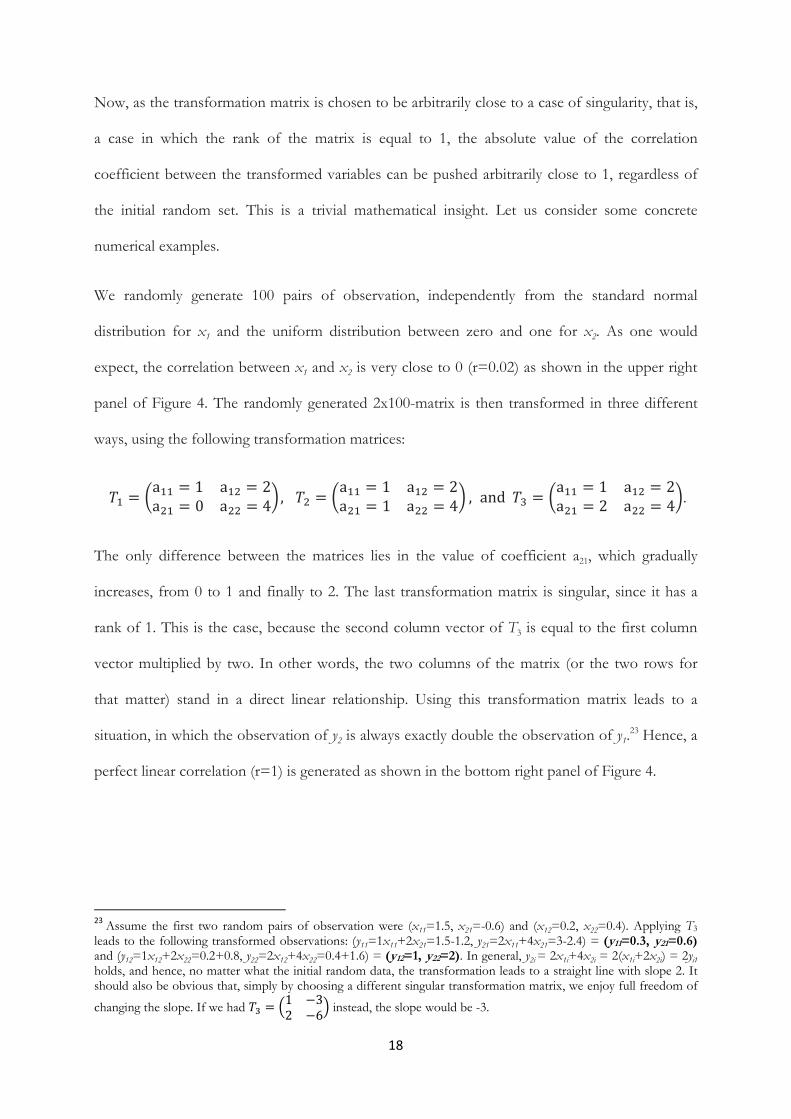
Now, as the transformation matrix is chosen to be arbitrarily close to a case of singularity, that is,

a case in which the rank of the matrix is equal to 1, the absolute value of the correlation

coefficient between the transformed variables can be pushed arbitrarily close to 1, regardless of

the initial random set. This is a trivial mathematical insight. Let us consider some concrete

numerical examples.

We randomly generate 100 pairs of observation, independently from the standard normal

distribution for x1 and the uniform distribution between zero and one for x2. As one would

expect, the correlation between x1 and x2 is very close to 0 (r=0.02) as shown in the upper right

panel of Figure 4. The randomly generated 2x100-matrix is then transformed in three different

ways, using the following transformation matrices:

�� = �a�� = 1 a�� = 2a�� = 0 a�� = 4�,�� = �a�� = 1 a�� = 2a�� = 1 a�� = 4� , and�� = �a�� = 1 a�� = 2a�� = 2 a�� = 4�.

The only difference between the matrices lies in the value of coefficient a21, which gradually

increases, from 0 to 1 and finally to 2. The last transformation matrix is singular, since it has a

rank of 1. This is the case, because the second column vector of T3 is equal to the first column

vector multiplied by two. In other words, the two columns of the matrix (or the two rows for

that matter) stand in a direct linear relationship. Using this transformation matrix leads to a

situation, in which the observation of y2 is always exactly double the observation of y1.23 Hence, a

perfect linear correlation (r=1) is generated as shown in the bottom right panel of Figure 4.

23

Assume the first two random pairs of observation were (x11=1.5, x21=-0.6) and (x12=0.2, x22=0.4). Applying T3 leads to the following transformed observations: (y11=1x11+2x21=1.5-1.2, y21=2x11+4x21=3-2.4) = (y11=0.3, y21=0.6)

and (y12=1x12+2x22=0.2+0.8, y22=2x12+4x22=0.4+1.6) = (y12=1, y22=2). In general, y2i = 2x1i+4x2i = 2(x1i+2x2i) = 2yi1 holds, and hence, no matter what the initial random data, the transformation leads to a straight line with slope 2. It should also be obvious that, simply by choosing a different singular transformation matrix, we enjoy full freedom of

changing the slope. If we had �� = �1 −32 −6� instead, the slope would be -3.

19

Figure 4: Numerical examples of linear transformations of a random set of observations

Upper left: random sample of size n=100, independently generated from the standard normal distribution for x1 and the uniform distribution between zero and one for x2; upper right: first transformation matrix T1 applied to sample; bottom left:

T2 applied to sample; bottom right: T3 (singular) applied to sample; r = Pearson’s correlation coefficient.

The transformations generated by T1 and T2 are intermediate cases. However, already the first

transformation leads, from a case of no correlation (original random sample), to one in which the

correlation coefficient has increased to r=0.87, which would be considered a fairly strong

empirical relationship by any social scientist. The second transformation matrix as it approaches

the special case of singularity leads to an even higher correlation of 0.97.

20

Now, what are the conclusions that Ragnar Frisch draws from this trivial mathematical insight?

At first, he declares:

It is clear that if the Jacobian [the transformation matrix] […] is singular, something important

happens. In this case the distribution of y1 and y2 in a (y1y2) diagram is at most one-dimensional,

and this happens regardless of what the individual observations x1 and x2 are - even if the

distribution in the (x1x2) diagram is a completely chaotic distribution. […]

[…] the essence of the situation is that even if the observations x1 and x2 are spread all over the

(x1x2) diagram in any way whatsoever, for instance in a purely chaotic way, the corresponding

values of y1 and y2 will lie on a straight line in the (y1y2) diagram when the transformation matrix

is of rank 1. If the slope of this straight line is finite and different from zero, it is very tempting

to interpret y1 as the “cause” of y2 or vice versa. This “cause”, however, is not a manifestation

of something intrinsic in the distribution of x1 and x2, but is only a human figment, a human

device, due to the special form of the transformation used. (Frisch 1970a, p. 13)

Frisch does not provide a numerical example to illustrate his point, which helps in keeping up the

appearance of scientific sophistication. In fact, it is absolutely inadequate to talk about something

like a “cause” at all. Sticking to our previous numerical example, the transformed variable y2 will

always be exactly equal to y1 multiplied by two, by definition. The transformation is equivalent to

merging the two initial random variables into one, and then defining the other as the merged

variable times two. It really boils down to saying that y1 is the cause of 2y1, which is, whatever y1

may stand for, not an explanation of variable y2 (= 2y1), but a mere definitional tautology.

More importantly, the singular transformations y1 and y2 have completely lost their relation to the

initial random data. There is no way to get back from the transformed data to the original

random sample, since one dimension, that is half of the complexity, has simply been erased from

the picture. The singularity of T3 means that there exists no inverse matrix, T3-1, such that T3 T3

-1

= I, where I denotes the 2x2 identity matrix. 24 Hence, there is no matrix, which could be

multiplied by the transformed data set in order to obtain the original random sample. So, if (x1,

24

The transformation matrices T1 and T2 have inverse matrices, so that it is always possible to go back to the initial data from the transformations. For example:

������ = �1 20 4� �1 −1 2�0 1 4� = �1 00 1� = �.

21

x2) is the underlying “ultimate reality”, as Frisch likes to think about it in his metaphor, then, the

singular transformation (y1, y2), which has generated perfect order out of chaos, seems to be

rather useless as it has completely lost its connection to this reality. A conclusion drawn from the

transformed data would have no real meaning.

But what if the transformation is not singular? Frisch (1970a, p. 14) explains:

Suppose that the distribution of (x1x2) is unknown and arbitrary with the only proviso that it

shall not degenerate into a straight line […]. We can then indicate a nonsingular linear

transformation of the variables x1 and x2 which produce as strong a correlation in (y1y2) as we please.

This is true because we can choose a transformation matrix, which is infinitesimally close to a

singular matrix, but not quite yet there. It has been illustrated in Figure 4. In such a situation the

transformed data preserves all the complexity of the initial random sample and it can always be

retransformed by inversion. Yet, the apparent structure that has been created is again only of a

tautological nature. By definition, the transformed data is created out of the same elementary

factors x1 and x2. We can generalize our numerical example as follows:

y1=1x1+(2-ε)x2 and y2=2(x1+2x2).

Obviously, as ε tends toward zero, that is, as the transformation matrix approaches singularity, y2

approaches 2y1 and their correlation coefficient tends towards 1.

Be that as it may. Even accepting Frisch’s metaphor so far and assuming that the transformation

in effect provides us with a meaningful relationship that seems to be, in some way or another,

exploitable for the betterment of humankind in a fundamentally chaotic “ultimate reality”, there

remains another fundamental problem. What happens when chaos changes its mind? If the

ultimate reality really is chaotic, any nonsingular transformation that has previously led to a

sufficiently strong empirical relationship might explode if chaos has its way.

22

Let us illustrate the point as well as we can.25 Assume that the transformation T1 had been found

by painstaking scientific enquiry by the most brilliant minds in Frisch’s metaphorical world.

Given the data shown in the upper left panel of Figure 4, the scientists have unleashed an

underlying empirical relationship (r=87) by using T1, that seems to be robust after repeated

testing.26 The point of the following example is to show, that this scientific success was possible

only in so far as the underlying “ultimate reality” was ordered in some sense in the first place, and

hence not fundamentally chaotic.

Notice again, the generation of the random data set in Figure 4 was based on the standard normal

distribution, which has a mean of zero and a standard deviation of one, for variable x1, and the

uniform distribution between the lower bound of zero and the upper bound of one for variable

x2. In other words, the parameters, which determine the exact shape of the probability

distributions, have been fixed beforehand. Now what if “real chaos” sets in and the parameters

of the distributions, that is, the mean and the standard deviation of the normal distribution as

well as the lower and upper bounds of the uniform distribution, become random variables

themselves?

Figure 5 shows an illustrative example. The second random set also contains n=100 observations

for both variables from the same families of probability distributions. After every 10th pair of

observation, the configuration of the distribution parameters has randomly changed.27 As a result,

25

One has to keep in mind, that we, as human beings, are simply not capable of purposefully creating chaos. It might look like chaos on the surface, but there is always an underlying deterministic structure. For the sample in the above example (Figure 4), I have used the programming language R (see Appendix), which generates pseudo-random numbers using the Mersenne-Twister based on the Mersenne prime number 219937 – 1. This pseudo-random number generator has been developed by Matsumoto and Nishimura (1998). The same process is used for the following example (Figure 5). 26

In fact, simulating the exact scenario from Figure 4 repetitively (1,000 times), has shown that in 96% of the cases the correlation coefficient after transformation T1 is larger than 0.82. It has never been lower than 0.76. 27

For the simulation of variable x1, the mean of the normal distribution has been randomly selected (with replacement) from the integers between -25 and +25. The standard deviation has been randomly selected (with replacement) from the integers between 1 and 10. Both parameters have been randomly changed after every 10th observation. For variable x2, the lower bound of the uniform distribution has been randomly selected (with replacement) from the integers between -25 and 25, the upper bound has then been randomly fixed between 1 to 10 integers above the lower bound (again random selection with replacement). After every 10th observation the bounds

23

the correlation coefficient after transformation of the random set has reduced from 0.87 to a

mere 0.15. The previously robust empirical relationship between y1 and y2 has vanished.28

Figure 5: Comparison of the same transformation for different random sets

Left panel: corresponds to the upper right panel of Figure 4; right panel: the same transformation matrix, T1, has been applied to different random data set, generated by the underlying probabilistic mechanism described in footnote 27.

The sobering conclusion from this little simulation exercise is that statistical induction from

empirical observations requires some structure, i.e. some constants that do not change. In a

“chaotic” world, where there are no such constants, we can obtain structure only by using a

singular transformation, that is, by ignoring the true nature of the world, or the subject matter,

whatever the field of scientific enquiry may be. Had the scientists in the Frischian world

inductively concluded that they found a true law, a constant, structural and quantitative

relationship between y1 and y2, and had possible social, economic, or political conclusions been

drawn on the basis of that relationship, who knows where it would lead to when the structural

change sets in? This change has been illustrated by the passage to a different simulation

have been randomly changed. After the simulation of a sample of size n=100, all observations have been divided by 10, in order to bring them roughly onto the same scale as the observations in the previous simulation. 28

Now, it is clear that in principle, the resulting correlation coefficient could also be higher than 0.87. The point is, that one can never know, if there is a “chaotic” underlying structure. However, repetitive simulations (1,000 times) show that more than half of the time (53.7%) the correlation coefficient is below 0.5, and in only 0.4% of the simulations it is above 0.87.

24

mechanism in which the parameters of the probability distributions have become random

variables themselves.

In his example, Frisch regards the transformations as representing the progress of the sciences in

finding regularities:

Science considers it a triumph whenever it has been able by some partial transformation here

or there, to discover new and stronger regularities. If such partial transformations are piled one

upon the other, science will help the biological evolution towards the survival of that kind of

man that in the course of the millenniums is more successful in producing regularities. If “the

ultimate reality” is chaotic, the sum total of the evolution over time - biological and scientific -

would tend in the direction of producing a mammoth singular transformation which would in

the end place man in a world of regularities. (Frisch 1970a, p. 15)

In his vision, Frisch sees man as being capable of creating reality himself, independent of the

constraints that some underlying “ultimate reality” may have. This really seems to be a matter of

semantics. One might counter with a simple stipulation, which even has a slight instrumentalist

notion: all creations of man, that serve their purpose, and a fortiori, all creational powers of man,

must be rooted in reality. It has been pointed out above that, within the boundaries of Frisch’s

example, any singular transformation loses its relation to the initial data set. It loses its relation to

reality, so to speak. A “mammoth singular transformation”, under these circumstances, seems to

be a rather scary idea.

The above simulation examples are just an illustration of the critique that Austrian economists

have leveled against the modern mainstream conception of econometrics (Hoppe 1983, 2006

[1993], ch. 10, 2007 [1995], 2010 [1988], ch. 6; Mises 1933, 1962, 2007 [1957]). The essence of

their critique is that inductive statistical methods require some constancy in the way that

perceived causal factors exert their effects, in very much the same way as the robustness of the

empirical finding in the first simulation example, depended on the constancy of the parameters of

the underlying probability distributions. For inductive statistical analysis, that is some kind of

verification or falsification of hypothetical-theoretical statements, to be possible in the first place,

25

the constancy principle must be satisfied. It holds that the same observable causes always lead to the same

observable effect and that different effects must be the result of different causes (Hoppe 1983, p. 11).

Whether we think of “cause” merely as a “human device” as Frisch suggested, or something

more fundamental, is irrelevant.

Now, to the extent that the constancy principle is not actually satisfied, but is simply assumed to

be true, the scientist runs the risk of drawing conclusions that are unwarranted, which is of

particular importance in politically relevant fields such as economics, not so much in a field like

astronomy. Formulating economic theory based on quantitative models in order to derive

quantitative economic relationships, testing those relationships and thereby assuming constancy

in one way or another may be seen as a kind of approximation from the true complexity of the

underlying problem. It is of utmost importance to think about the consequences of such

approximations. In order to do that, one has to reflect on the nature of the underlying problem

that is approximated.

In fact, Frisch conceived of econometrics as being essentially an approximation. In a letter to F.

C. Mills from 21 February 1928, he explains in a somewhat peculiar manner:

We engage in this kind of approximation work without knowing exactly what we are trying to

approximate. We engage seriously in target shooting without having any target to shoot at. The

target has to be furnished by axiomatic economics. The axiomatic process of target making

must necessarily be rather abstract, a fact which accounts, perhaps, for its lack of popularity in

these days when it is considered quite a virtue to disregard abstract thinking in economics. It is

abstract, but neither in the sense of a logic game nor in the sense of metaphysical verbiage, of

which we have had some in economics, at times. Axiomatic economics will construct its

quantitative notions in the same way as theoretical physics has constructed its quantitative

notions. (cited in Bjerkholt and Dupont 2010, pp. 31-32)

Frisch is giving the impression that the mathematical axiomatization of economic theory29 is a

free floating concept, detached from reality, a veritable singular transformation. Yet, it clearly serves

29

It is not to be confused with the axiomatization in the tradition of the Austrian school, which came to full fruition in Rothbard (2009 [1962], p. lvi), who claims:

26

the purpose of describing human behavior and action. By extension, this is exactly what Frischian

econometrics tries to approximate. It tries to accomplish this approximation by mathematically

relating some quantifiable external factors, which it conceives of as the causes, to some other

quantifiable external factors, which are seen as the effects of human action. For what lies between

the causes and the effects, namely the human actor, it makes a constancy assumption, where it is

not actually satisfied.

This is not to argue about the puzzling question of free will (Rothbard 2011, ch. 1). It might be

true that human action from some remote point of view is in fact completely determined, taken

all possible causal factors into account (Mises 2007 [1957], p. 1). However, it is simply not the

case, that a certain configuration of those “causal factors” that are commonly considered in

econometrics always leads to the same actions, or at least to the same changes in the external

world, as results of possibly different actions – not even on average or in some other probabilistic

sense. Modern econometrics is only capable of working on a rather superficial level of accuracy,

given the amount and diversity of potential causal factors that could shape human action and that

are completely out of reach for the econometrician and for any other scientist. On this level,

substantial structural change is a well known empirical fact.30

The present work deduces the entire corpus of economics from a few simple and apodictically true axioms: the Fundamental Axiom of action – that men employ means to achieve ends, and two subsidiary postulates: that there is a variety of human and natural resources, and that leisure is a consumers’ good.

In fact, this might exactly be the kind of “metaphysical verbiage” that Frisch refers to. Action itself is an

unobservable concept, and hence, useless from the point of view of Frischian econometrics. Certain consequences of

actions are observable, such as the movement of the human body or the rearrangement of objects in the external

world, not action itself.

30 One of the most prominent and important cases in modern macroeconomics that provide a well-known example

for what has been considered a structural change, is the relationship between price inflation and unemployment. The stagflation of the 1970s has led to a rejection of the large-scale Keynesian macroeconometric models à la Evans and Klein (1967), Klein and Goldberger (1955) or Klein (1964) that were essentially elaborated IS-LM models augmented with a politically exploitable Phillips Curve (Webb 1999). Interestingly, Hurtado (2014) gathered empirical evidence that the modern New Classical and New Keynesian DSGE models (Galí and Gertler 2007; Galí 2008; Woodford 2003) that emerged out of the New Classical Critique (Lucas 1983 [1976]) would not have performed much better, if they had been used back in the 1970s instead of the old models. True enough, those models suffer from the same fundamental problems.

27

Not the verification or falsification of economic theory, that is, the generalization of empirical

facts, but rather the finding of empirical facts is the proper role of econometrics. As long as

modern econometricians engage in unwarranted generalizations, the “cycles of empiricism and

rationalism” in economics that Frisch (1930) refers to are likely to continue. Sooner or later those

generalizations may yield unsatisfactory conditions if put into practice, which induces a

renunciation from empiricism, in the same way as deranged theoretical propositions may induce a

return to empiricism. Frisch himself has seen the danger of econometrics becoming more of a

“playometrics” (Frisch 1970a).

The “new fusion of theory and observation” that Frisch called for could be found in a purely

descriptive econometrics, that recovers the empirical facts and problems, which then have to be

explained by economic theory. A particularly important field for econometrics would then be

economic history (Mises 2007 [1957]). Many of the statistical techniques that modern

econometricians have developed are completely compatible with such a more Ciompanian

conception of econometrics. In particular, his broader conception of economographics as

“descriptive economics” could be developed further into this direction.

Concluding Remarks

In the first part of this paper, Pawel Ciompa’s (1910) concept of a purely descriptive

econometrics that is closely related to the theory of accounting has been presented. It is

important to notice that econometrics for Ciompa was a mere application of economic theory,

not a way to develop it further. In sharp contrast, the modern Frischian conception of

econometrics, which has been discussed subsequently, calls for a reformulation, even a genuine

transformation, of economic theory in mathematical and quantifiable terms. One essential role of

statistical analysis (the empirical-quantitative) within this modern conception is the verification or

falsification of theoretical propositions (the theoretical-quantitative). Picking up an example from

28

Frisch’s epistemological reflections, computer simulations have been used in order to illustrate

the central point of criticism that economists of the Austrian school have leveled against the

modern econometric approach. These economists have noticed that the necessary condition for

inductive statistical analysis is the constancy principle. There is ample reason to question the validity

of this principle for the problems that econometrics typically deals with, at least on the rather

superficial level of detail and accuracy that it is capable of achieving.

Although the two conceptions share a common element, namely the descriptive side of statistical

analysis, it is the inductive side of modern econometrics that puts them far apart. Even from

Frisch’s own perspective, it is clear that modern econometrics is an approximization as many

other scientific enquiries. The crucial question is of course, how far should one approximate?

How much are we willing to abstract from what is considered to be real? The answer to this

question may lie outside of the confines of the discipline of economics itself.

It was Joseph A. Schumpeter (2006 [1954], part I, ch. 4) in his History of Economic Analysis, who

stressed the role and inevitability of ideology in economic analysis. According to him ideology

enters economic analysis at the very start, in the “preanalytic cognitive act that supplies the raw

material for the analytic efforts”, which he would also refer to as the “Vision.” (p. 39)

Schumpeter explains:

Analytic work begins with material provided by our vision of things, and this vision is

ideological almost by definition. It embodies the picture of things as we see them, and

wherever there is any possible motive for wishing to see them in a given rather than another

light, the way in which we see things can hardly be distinguished from the way in which we

wish to see them. (p. 40)

It thus seems as if the question that we have dealt with at the heart of this paper is precisely one

of ideology or vision. How do we look at the world, and more importantly, how do we look at

man?

29

Ragnar Frisch was convinced that econometrics is in fact a set of tools for solving social and

economic problems (Frisch 1944) as it provides the guidelines for economic planning. Having

Pawel Ciompa’s vision of econometrics and economographics, as a descriptive economics, in

mind, I would suggest that it should rather be seen as a set of tools for identifying and describing

the empirical manifestations of social and economic problems, nothing more and nothing less.

The solution of these problems, if they are solvable at all, must ultimately come from reason.

30

Bibliography

Aspers, Patrik. 2001. “Crossing the Boundary of Economics and Sociology: The Case of Vilfredo Pareto.” The American Journal of Economics and Sociology 60(2): 519–45.

Bjerkholt, Olav. 1995. “Ragnar Frisch: The Originator of Econometrics.” In Foundations of Modern Econometrics: The Selected Essays of Ragnar Frisch, ed. Olav Bjerkholt. London: Edward Elgar.

Bjerkholt, Olav, and Ariane Dupont. 2010. “Ragnar Frisch’s Conception of Econometrics.” History of Political Economy 42(1): 21–73.

Böhm-Bawerk, Eugen von. 1930. The Positive Theory of Capital. New York: G. E. Stechert and Co.

Chipman, John S., ed. 1971. Preferences, Utility, and Demand: A Minnesota Symposium. New York: Harcourt Brace Jovanovich.

Ciompa, Pawel. 1910. Grundrisse einer Oekonometrie und die auf der Nationaloekonomie aufgebaute natiurliche Theorie der Buchhaltung: ein auf Grund neuer ökonometrischer Gleichungen erbrachter Beweis, dass alle heutigen Bilanzen falsch dargestellt werden. Lviv (Lemberg): Artur Goldman.

Evans, Michael K., and Lawrence R. Klein. 1967. The Wharton Econometric Forecasting Model. University of Pennsylvania: Wharton School of Finance and Commerce.

Fisher, Irving. 1892. Mathematical Investigations in the Theory of Value and Prices. Transactios of the Connecticut Academy, VOL. IX.

Friedman, Milton. 2008. “The Methodology of Positive Economics.” In The Philosophy of Economics - An Anthology, ed. Daniel M. Hausman. Cambridge: Cambridge University Press, 145–78.

Frisch, Ragnar. 1926a. Sur les semi-invariants et moments employés dans l’étude des distributions statistiques. Oslo: Norwegian Academy of Science, Part II: History and philosophy, nr. 3.

———. 1926b. “Sur un problème d’économie pure.” Norsk Matematisk Forenings Skrifter Series 1(16): 1–40.

———. 1930. “A Dynamic Approach to Economic Theory.” Lectures at Yale University beginning September 1930. Typewritten manuscript, Frisch Archive, Department of Economics, University of Oslo.

———. 1933. “Editor’s Note.” Econometrica 1(1): 1–4.

———. 1936. “Note on the Term ‘Econometrics.’” Econometrica 4(1): 95.

———. 1944. “The Responsibility of the Econometrician.” Econometrica 14(1): 1–4.

———. 1950. “Alfred Marshall’s Theory of Value.” The Quarterly Journal of Economics 64(4): 495–524.

———. 1952. “Frisch on Wicksell.” In The Development of Economic Thought, ed. Henry William. New York: Spiegel, 652–99.

———. 1957. “Sur un problème d’économie pure.” Metroeconomica 9(2): 79–111.

———. 1970a. “Econometrics in the World Today.” In Induction, Growth, and Trade: Essays in Honour of Sir Roy Harrod, eds. W. A. Eltis, F. Scott, and J. N. Wolfe. Oxford: Clarendon Press, 152–66.

———. 1970b. “From Utopian Theory to Practical Applications: The Case of Econometrics.” Lecture to the memory of Alfred Nobel.

———. 1970c. “Ragnar Anton Kittil Frisch.” Les Prix Nobel 1969: 204–6.

———. 2013. Problems and Methods of Econometrics: The Poincaré Lectures of Ragnar Frisch, 1933. eds. Olav Bjerkholt and Ariane Dupont-Kieffer. New York: Routledge.

Galí, Jordi. 2008. Monetary Policy, Inflation, and the Business Cycle: An Introduction to the New Keynesian Framework. Princeton and Oxford: Princeton University Press.

Galí, Jordi, and Mark Gertler. 2007. “Macroeconomic Modeling for Monetary Policy Evaluation.” Journal of Economic Perspectives 21(4): 25–45.

Hausman, Daniel M. 2008. The Philosophy of Economics - An Anthology. 3rd ed. ed. Daniel M. Hausman. Cambridge: Cambridge University Press.

31

Hoppe, Hans-Hermann. 1983. Kritik der kausalwissenschafilichen Sozialforschung - Untersuchungen zur Grundlegung von Soziologie und Ökonomie. Opladen: Westdeutscher Verlag.

———. 2006. The Economics and Ethics of Private Property: Studies in Political Economy and Philosophy. Auburn, AL: Ludwig von Mises Institute.

———. 2007. Economic Science and the Austrian Method. Auburn, AL: Ludwig von Mises Institute.

———. 2010. A Theory of Socialism and Capitalism. Auburn, AL: Ludwig von Mises Institute.

Hülsmann, Jörg Guido. 2003. “Facts and Counterfactuals in Economic Law.” Journal of Libertarian Studies 17(1): 57–102.

Hurtado, Samuel. 2014. “DSGE Models and the Lucas Critique.” Economic Modelling 44: S12–19.

Jaffé, William. 1976. “Menger, Jevons and Walras de-homogenized.” Economic Inquiry XIV(4): 511–24.

Jevons, William Stanley. 1965. Theory of Political Economy. 5th ed. New York: Augustus M. Kelley.

Klein, Lawrence R. 1964. “A Postwar Quarterly Model: Description and Applications.” In Models of Income Determination, Princeton University Press, 11–58.

Klein, Lawrence R., and Arthur S. Goldberger. 1955. An Econometric Model of the United States, 1929-1952. Amsterdam: North-Holland Publishing Company.

Lucas, Robert E. 1983. “Econometric Policy Evaluation: A Critique.” In Theory, Policy, Institutions: Papers from the Carnegie-Rochester Conference Series on Public Policy, eds. Karl Brunner and Alan Meltzer. North-Holland: Elsevier Science Publishers B.V., 257–84.

Matsumoto, M., and T. Nishimura. 1998. “Mersenne Twister: A 623-Dimensionally Equidistributed Uniform Pseudo-Random Number Generator.” ACM Transactions on Modeling and Computer Simulation 8(1): 3–30.

Mattessich, Richard. 2008. Two Hundred Years of Accounting Research: An International Survey of Personalities, Ideas and Publications. Abingdon and New York: Routledge - Taylor and Francis Group.

Menger, Carl. 2007. Principles of Economics. Auburn, AL: Ludwig von Mises Institute.

Mises, Ludwig von. 1933. Grundprobleme der Nationalökonomie: Untersuchungen über Verfahren, Aufgaben und Inhalt der Wirtschafts- und Gesellschaftslehre. Jena: Verlag von Gustav Fischer (PDF-Version von Gerhard Grasruck für www.mises.de).

———. 1962. The Ultimate Foundation of Economic Science - An Essay on Method. New York: D. Van Nostrand Company, Inc.

———. 2007. Theory and History: An Interpretation of Social and Economic Evolution. Auburn, AL: Ludwig von Mises Institute.

Pufendorf, Samuel von. 1744. De jure naturae et gentium: libri octo. Frankfurt and Leipzig.

Rothbard, Murray N. 2006. Economic Thought Before Adam Smith: An Austrian Perspective on the History of Economic Thought Volume I. Auburn, AL: Ludwig von Mises Institute.

———. 2009. Man, Economy, and State: A Treatise on Economic Principles - With Power and Market: Government and the Economy. Auburn, AL: Ludwig von Mises Institute.

———. 2011. Economic Controversies. Auburn, AL: Ludwig von Mises Institute.

Schumpeter, Joseph A. 2006. History of Economic Analysis. Routledge - Taylor and Francis e-Library.

Walras, Léon. 1874. Éléments d’économie politique pure (Théorie de la richesse sociale). Lausanne: L. Cordaz.

Webb, Roy H. 1999. “Two Approaches to Macroeconomic Forecasting.” Economic Quarterly-Federal Reserve Bank of Richmond 85(3): 23–40.

Wiśniewski, Jerzy Witold. 2016. Microeconometrics in Business Management. Chichester: John Wiley and Sons, Ltd.

Woodford, Michael. 2003. Interest and Prices: Foundations of a Theory of Monetary Policy. Princeton and Oxford: Princeton University Press.

Les autres documents de travail du GRANEM accessibles sur le site Web du laboratoire à l’adresse suivante : (www.univ-angers.fr/granem/publications) :

Numéro Titre Auteur(s) Discipline Date

2008-01-001 The Cognitive consistency, the endowment effect and the preference reversal phenomenon

Serge Blondel, Louis Lévy-Garboua Théorie du Risque octobre 2008

2008-02-002 Volatility transmission and volatility impulse response functions in European electricity forward markets

Yannick Le Pen, Benoît Sévi Econométrie Appliquée octobre 2008

2008-03-003 Anomalies et paradoxes dans le cas des choix alimentaires : et si les carottes n’étaient pas oranges ?

Serge Blondel, Christophe Daniel, Mahsa Javaheri

Economie Expérimentale octobre 2008

2008-04-004 The effects of spatial spillovers on the provision of urban environmental amenities

Johanna Choumert, Walid Oueslati, Julien Salanié

Economie du Paysage octobre 2008

2008-05-005 Why do rational people vote in large elections with costs to vote?

Serge Blondel, Louis Lévy-Garboua Théorie du Risque novembre 2008

2008-06-006 Salaires, conditions et satisfaction au travail Christophe Daniel Economie du Travail novembre 2008

2008-07-007 Construction communicationnelle du stock de connaissances de la compétence collective – Contribution à partir d’une conversation.

Nicolas Arnaud Gestion des Ressources Humaines décembre 2008

2008-08-008 On the non-convergence of energy intensities: evidence from a pair-wise econometric approach

Yannick Le Pen, Benoît Sévi Econométrie Appliquée décembre 2008

2008-09-009 Production of Business Ethics Guido Hülsmann Economie Politique décembre 2008

2008-10-010 Time preference and investment expenditure Guido Hülsmann Economie Politique décembre 2008

2008-11-011 Le marché de la photographie contemporaine est-il soluble dans celui de l'art contemporain ?

Dominique Sagot-Duvauroux Economie de la Culture décembre 2008

2008-12-012 The newsvendor problem under multiplicative background risk

Benoît Sévi Microéconomie de l’Incertain décembre 2008

2009-01-013 Complémentarité de la collaboration électronique et de l’investissement relationnel : étude de cas exploratoire d’un SIIO dans le secteur du meuble

Redouane Elamrani, Nicolas Arnaud Organisation avril 2009

2009-02-014 On the realized volatility of the ECX CO2 emissions 2008 futures contract: distribution, dynamics and forecasting

Julien Chevallier, Benoît Sévi Finance mai 2009

2009-03-015 The communicational making of a relation-specific skill: contributions based on the analysis of a conversation to strategy-as-practice and resource-based view perspectives

Nicolas Arnaud Stratégie juin 2009

2009-04-016 Le droit d'auteur, incitation à la création ou frein à la diffusion ? Une analyse empirique du cas de la création télévisuelle

Françoise Benhamou, Stéphanie Peltier Economie de la Culture septembre 2009

2009-05-017 Diversity analysis in cultural economics: theoretical and empirical considerations

Françoise Benhamou, Renato G. Flôres Jr., Stéphanie Peltier

Economie de la Culture septembre 2009

2009-06-018 L’épargne retraite en entreprise : un état des lieux au regard de l’expérience américaine

Fabrice Pansard, Bruno Séjourné Finance septembre 2009

2009-07-019 Options introduction and volatility in the EU ETS Julien Chevallier, Yannick Le Pen, Benoît Sévi

Econométrie Appliquée septembre 2009

2009-08-020 Modeling strategic interactions between firms and local authorities – The case of a biotechnology cluster

Alain Berro, Isabelle Leroux Economie des réseaux septembre 2009

2009-09-021

The strategy adopted by non-profit care services organizations in dealing with the new French regulatory system: strategic coalitions and reterritorialisation of activities

Isabelle Leroux, Laurent Pujol, Eric Rigamonti

Economie Sociale novembre 2009

2009-10-022 Une nouvelle lecture du territoire par la limite Jean-Claude Taddei Territoire novembre 2009

2010-01-023 Adoption of new identity-based services: Proposition of a conceptual model based on TAM, DOI and perceived risks

Caroline Lancelot Miltgen e-marketing juillet 2010

2010-02-024

Young Europeans’ motivations, perceived risks and requirements regarding electronic identification : Some comparative results from focus groups in four EU27 countries

Caroline Lancelot Miltgen e-marketing décembre 2010

2010-03-025 Analyse du risque de non-exécution des ordres à la bourse de Paris

Angélique Aubier Piron Finance décembre 2010

2011-01-026 Who cares? Europeans’ attitudes towards the disclosure of personal identity data

Caroline Lancelot Miltgen, Margherita Bacigalupo, Wainer Lusoli

Systèmes d'information et e-marketing

janvier 2011

2011-02-027 Le rôle des Business Angels dans le financement de l’innovation radicale.

Catherine Deffains-Crapsky Finance entrepreneuriale avril 2011

2011-03-028 The EU Financial Reform facing the Global Context Dominique Perrut Economie financière mai 2011

2011-04-029 A simple test of the sustainable development hypothesis Serge Blondel Economie expérimentale septembre 2011

2011-05-030 Evaluation d’un nouveau produit alimentaire : le rôle de la congruence et du packaging

Gaëlle Pantin-Sohier et Caroline Lancelot Miltgen

Comportement du consommateur octobre 2011

2011-06-031 Une mesure de risque extrême agrégée : risque de marché et risque de liquidité

Angélique Aubier-Piron Finance octobre 2011

2011-07-032 When should a French Investor use a Dollar-Cost Averaging Strategy?

Philippe Compaire et Bruno Séjourné Finance octobre 2011

2011-08-033 Conformisme à la norme et performance : la franchise dans le mix organisationnel

Christophe Daniel, Regis Dumoulin et Claire Gauzente

Stratégie et organisation octobre 2011

2011-09-034 The structure of production reconsidered Guido Hülsmann Economie politique décembre 2011

2012-01-035 The quality of private monitoring in European banking: completing the picture

Adrian Pop et Diana Pop Economie financière février 2012

2012-02-036 Urban sprawl occurrence under spatially varying agricultural bid-rent and amenities

Thomas Coisnon, Walid Oueslat et Julien Salanié

Economie urbaine septembre 2012

2012-01-037 Le renouveau du paiement du dividende en actions Caroline Marie-Jeanne Finance mars 2012

2013-01-038 Spatial targeting of agri-environmental policy and urban development

Thomas Coisnon, Walid Oueslat et Julien Salanié

Economie urbaine février 2013

2013-02-039 Fiat money and the distribution of incomes and wealth Jörg Guido Hülsmann Economie politique novembre 2013

2014-01-040 Determinants of urban sprawl in European cities Walid Oueslati, Seraphim Alvanides et Guy Garrodc

Economie urbaine janvier 2014

2014-02-041 Financial markets and the production of law Jörg Guido Hülsmann Economie politique juin 2014

2014-03-042 Organisation des filières bananes ivoiriennes : Une étude de terrain expérimentale

Serge Blondel, Rodrigue Brin et Camille Koffi

Economie expérimentale septembre 2014

2014-04-043 How fair are the fair price standards in blockholder regimes?

Adrian Pop et Diana Pop Finance septembre 2014

2015-01-044 The nature and impacts of environmental spillovers on housing prices: A spatial hedonic analysis

Masha Maslianskaia-Pautrel et Catherine Baumont

Economie de l’environnement février 2015

2015-02-045 The old economics of science, the nonlinear model of innovation, and the economics of patents

Matthieu Ballandonne Histoire de la pensée économique mai 2015

2015-03-046 How private happiness involves greater economic and social efficiency? A New paradigm adapted to the world knowledge economy

Camille Baulant Intelligence économique novembre 2015

2016-01-047 Les déterminants de la syndication avec les Business Angels dans les opérations d’Equity Crowdfunding : Le cas français

Catherine Deffains-Crapsky, Thibault Cuenoud et Pascal Glemain

Finance mai 2016

2016-02-048 A matter of trust and time: Back to the adoption of embeddedness in economic geography (1985-2015)

Florian Fougy et Sylvain Amisse Histoire de la pensée économique mai 2016

2016-03-049 Cultural consequences of monetary interventions Jörg Guido Hülsmann Economie politique septembre 2016

2016-04-050 In the long run we are all unemployed Karl-Friedrich Israel Economie politique septembre 2016

2016-05-051 Les critiques libérales du service public Jörg Guido Hülsmann Economie politique septembre 2016

2016-06-052 Pawel Ciompa and the meaning of econometrics: A comparison of two concepts

Karl-Friedrich Israel Economie politique septembre 2016