MISSOURI DEPARTMENT OF TRANSPORTATION

PAVEMENT DESIGN AND TYPE SELECTION PROCESS

PHASE I REPORT

March 2, 2004

Review Conducted by MoDOT/Industry

1

Preface

This report has been developed to show the history of the MoDOT pavement design and type selection process and where the process is going in the future. The transparency of this process was intended to enlighten transportation users in Missouri and ensure MoDOT accountability in adhering to the process. The report contains recommendations by the Pavement Team for various pavement design and type selection issues. These recommendations were not always reached by consensus of the Team, which included asphalt and concrete paving industry representatives, as well as MoDOT and FHWA representatives, because consensus could not be reached on all issues. In those cases MoDOT management made policy decisions based on the best data available at the time. In closing, the Pavement Design and Type Selection Process is a very contentious issue all over the country. Almost every DOT is dealing with this issue in some form. There are no easy answers. However, MoDOT is committed to keeping abreast of technology changes and using industry resources to continually improve the Pavement Design and Selection Process, so that, ultimately, the people who use our transportation system are the benefactors. If anyone wants to learn more about MoDOT’s Pavement Design and Type Selection Process, they can contact MoDOT at http://www.modot.org, or call 1-888-ASK-MODOT.

2

Executive Summary

Faced with deteriorating pavements on one of the nation’s largest state highway systems, inadequate fiscal resources and public demand for improved roadways, the Missouri Department of Transportation embarked on a project more than a year ago to ultimately improve the condition of its primary routes while providing the best pavement value to the citizens of Missouri. The initial impetus for forming a Pavement Design and Type Selection Team was a report published by MoDOT’s Research, Development and Technology unit in 2002 – “Missouri Guide for Pavement Rehabilitation” – that analyzed the historical performance of various pavement types in Missouri. At the same time, data showed that only 35 percent of the National Highway System (NHS) in Missouri (and other primary arterials) was in good or better condition. And, with dwindling financial resources, MoDOT was looking for ways to maximize the use of its limited amounts of funds. So, in the fall of 2002, a Pavement Team was created. Its membership included representatives from MoDOT and the Federal Highway Administration, the Missouri Asphalt Paving Association and the American Concrete Paving Association, and asphalt and concrete paving contractors. The team was charged to provide the public and stakeholders with two desired outcomes:

o the best pavement product that can be delivered within available resources.

o a clear understanding of the pavement design and selection process. Pavement Team Members

MoDOT Industry Dave Nichols, Project Development Matt Ross, ACPA Mike Anderson, District 5 David Yates, MAPA Jay Bledsoe, Transportation Planning Roger Brown, Pace Construction John Donahue, RDT Paul Corr, Fred Weber Inc. Pat McDaniel, Construction & Materials Kim Wilson, Clarkson Construction Travis Koestner, Design Donnie Mantle, APAC Virgil Stiffler, FHWA

Mara Campbell, MoDOT - facilitator

3

Involving industry in the process was a key component of the effort, not necessarily with a hope of building consensus but rather in having industry at the table so that its representatives had a clear understanding of the process and how it was developed. Developing pavement strategies for MoDOT’s entire 32,000-mile system was not the goal. Prior to formation of the team a MoDOT policy decision was made to maintain 23,000 miles of collector roads with a conventional thin-lift resurfacing program. That meant the team could focus its attention on the 9,000 miles of the state system (27 percent) that carries 86 percent of the traffic.

MoDOT System by Classification

13%

14%

73%

NHS

Remaining ArterialsCollectors

Background Examining MoDOT’s pavement type selection process is nothing new. It’s been done internally a number of times – most recently in 1998. Those past efforts, however, were conducted with only minimal, if any, input and contribution from the paving industry. One of the problems faced in the past was a pervasive opinion among MoDOT District designers – those who actually put the projects together – that the time required to get a pavement type selection took too long and ultimately resulted in selection of the same pavement design as what existed on the previous project. Industry had a number of issues, too, foremost of which was what was seen as a secretive, exclusive process. Past MoDOT policy did not call for sharing its life cycle cost analysis or data on specific projects with industry. That led to a perception that MoDOT was biased towards one industry or the other. In the past, MoDOT has used an empirical pavement design method that is based on observations of performance in pavements with known dimensions and materials under specific climatic, geologic and traffic conditions. Industry felt that the use of this method led to overly conservative designs that led to Missouri having some of the thickest pavements in the country. Why Now? Both the Missouri Highways and Transportation Commission and MoDOT have heard the message loud and clear from the general public in all areas of the state – more dollars need to be invested in taking better care of Missouri’s existing system of highways and bridges. That recognition has resulted in changes to MoDOT’s strategic plan and to the revenue allocation strategies of the MHTC. Now there are only two major thrusts for the organization:

4

o Take better care of what we have.

o Finish what we’ve started.

Making headway in those two areas will build public trust, a critical step if Missourians are ever to fund its transportation system at a higher level. An initial step has been to set a modest improvement goal: that the percentage of Missouri’s NHS and principal arterials that are in good or better condition climb from 35 percent to 50 percent in the next 10 years. To do so while recognizing that MoDOT does not have the resources to build the ultimate solution everywhere requires a careful balancing act. On one hand, and heeding the wishes of the public, MoDOT would like to build long-term solutions that enable its crews and contractors to “Get In, Get Out and Stay Out.” On the other hand, though, less expensive solutions could allow MoDOT to make more immediate improvements to more miles of road – thereby reaching its goals more quickly, but the impact would be that we are out working on our roads more often. Outcomes One of the fundamental findings of the Pavement Team was that MoDOT add mechanistic qualities to its empirical design philosophy. Mechanistic-empirical (M-E) design methods use a mechanistic process to determine what stresses, strains and deflections a pavement will experience from external influences (i.e. load weight and location, temperature, etc.) and an empirical relationship to connect pavement response with pavement deterioration. Implementation of M-E pavement design will allow MoDOT to design the pavement with the right thickness for the specific conditions in each geographic area. The team identified a number of other innovative pavement solutions, such as better subgrade and base treatments to extend pavement life. Also, MoDOT will use better quality products to improve the life and durability of its pavements. Things like:

o Polymer Modified Asphalt (PMA) in our more heavily traveled Hot Mix Asphalt (HMA) overlays.

o Use of Stone Matrix Asphalt (SMA) mixes in our HMA overlays on Missouri’s interstates.

o Use of Traditional HMA overlays, where appropriate.

5

o HMA overlays on rubblized Portland cement concrete.

o Jointed Plain Concrete Pavement (JPCP).

o Unbonded JPCP overlays.

A critical team recommendation to provide the most competitive prices for road improvements is the use of alternate bidding for pavements. To that end, 20 projects have been identified to provide more data for analysis as to the potential savings that can be realized. Alternate bidding provides the opportunity for both asphalt and concrete contractors to bid on the two lowest cost designs head-to-head. It also brings more contractors to the bidding arena, which translates into more competition and ultimately lower cost to the taxpayer. As of December 2003, MoDOT had two months of lettings behind it in alternate bidding of test projects. Two projects were awarded to asphalt contractors and two projects were awarded to concrete contractors. All four of these projects had more bidders than would normally have been the case had MoDOT bid only one type of pavement. The bottom line is the bids received were very competitive when compared to MoDOT engineers’ cost estimates for these projects, which is in keeping with the team’s belief that alternate bidding can and will bring great value to projects. It should be noted, however, that there will be a limited number of projects where alternate bidding is not the right solution. For example, unique working conditions or very high traffic volumes could warrant that a specific pavement design and solution be defined.

The team’s work also underscored the importance of life cycle cost analysis (LCCA) – an economic assessment of competing pavement treatments considering all significant costs over the life of each alternative, expressed in equivalent dollars. The FHWA requires the LCAA process be used on the selection of long-term pavement solutions. MoDOT’s

Rte 63 - Boone County Rte 63 - Callaway County

ASPHALT CONCRETE

6

Design estimators are brought into the process to analyze pavement costs through their knowledge of the latest and most current prices. They will also make changes to the LCCA process as prices change and performance data changes for each pavement type. Next Steps To move past its Phase One recommendations, the team must transition to the new M-E pavement design model. This will require lab and field work to calibrate the M-E design program to Missouri conditions. A number of other technical issues, delineated below, also remain to be resolved. Ultimately, though, MoDOT will realize more variability in its pavement thickness, which will mean that more dollars are available to fund more projects. Outstanding Phase II issues:

• Finalize pavement performance standards criteria.

• Set evaluation criteria for composite pavements.

• Finalize what costs will be considered in LCCA, such as user costs, vehicle operation costs, etc.

• Determine salvage values for each design or rehabilitation strategy generated.

• Review the results from initial alternate bid pavement projects.

• Determine if alternate bids on pavements should be extended to rehabilitation projects where only thin HMA overlays have historically been used.

• Determine if staged construction is a valid design consideration.

• Determine if the design catalog to be generated should be on a project-by-project basis or on a

regional or statewide basis.

• Develop methods to track the PTS process and to keep industry involved in the process.

• Determine if noise impact and friction need to become pavement design considerations.

• Determine the cost effectiveness of full-depth shoulders.

• Determine if recycled pavement savings are tangible and should be included in LCCA.

• Evaluate aggregate base designs, including drainage.

• Determine how preventive maintenance fits in LCCA.

• Identify how to capture maintenance expenditures on pavements for use in LCCA.

7

Conclusion MoDOT is committed to bring the best value possible to its pavement solutions. MoDOT is committed to keeping the paving industry involved in its paving process as we work in partnership to bring transportation solutions to our customers. MoDOT recognizes that pavement design and the type selection process is dynamic and will change as more data is gathered and more lessons are learned.

8

Table of Contents

Preface......................................................................................................................................... 1 Executive Summary ............................................................................................................. 2 List of Tables......................................................................................................................... 10 List of Figures ....................................................................................................................... 10 List of Appendices.............................................................................................................. 11 Glossary of Acronyms and Abbreviations.............................................................. 12 Glossary of Definitions .................................................................................................... 13 Chapter One Pavement Team...................................................................................... 15 Chapter Two Pavement Type Selection Process ................................................ 17

2.0 Introduction................................................................................................................... 17 2.1 Existing Pavement Type Selection Process .................................................................. 17 2.2 Recommended Pavement Type Selection Process ....................................................... 17

Chapter Three Performance Standards....................................................................... 19 3.0 Introduction................................................................................................................... 19 3.1 Existing Performance Standards ................................................................................... 19 3.2 Recommended Performance Standards ........................................................................ 20 3.3 Fiscal Impact................................................................................................................. 20

Chapter Four Design Lives / Periods ........................................................................ 21 4.0 Introduction................................................................................................................... 21 4.1 Existing Design Lives/Periods...................................................................................... 21 4.2 Review of Missouri Historical Data ............................................................................. 21 4.3 Recommended Design Lives/Periods ........................................................................... 25 4.4 Fiscal Impact................................................................................................................. 27

Chapter Five Design Types .......................................................................................... 28 5.0 Introduction................................................................................................................... 28 5.1 Current Pavement Types............................................................................................... 28 5.2 Other Pavement Types Considered............................................................................... 30 5.3 Subgrade Stabilization .................................................................................................. 30 5.4 Base Courses................................................................................................................. 31 5.5 Recommended Pavement Types ................................................................................... 31 5.6 Fiscal Impact................................................................................................................. 34

Chapter Six Design Model ............................................................................................ 35 6.0 Introduction................................................................................................................... 35 6.1 Current Design Model................................................................................................... 35 6.2 Other Design Models .................................................................................................... 35 6.3 Recommended Design Model....................................................................................... 36 6.4 Fiscal Impact................................................................................................................. 36

Chapter Seven Life Cycle Cost Analysis................................................................... 37 7.0 Introduction................................................................................................................... 37 7.1 Current LCCA Procedure ............................................................................................. 37

9

7.2 Other LCCA Methods................................................................................................... 37 7.3 Recommended LCCA Procedures ................................................................................ 38 7.4 Fiscal Impact................................................................................................................. 38

Chapter Eight Alternate Bidding for Pavements ................................................... 39 8.0 Introduction................................................................................................................... 39 8.1 Missouri Experience ..................................................................................................... 39 8.2 Alternate Bidding Issues ............................................................................................... 39

8.2.1 Method of Payment............................................................................................... 40 8.2.2 Quality Control / Quality Assurance..................................................................... 40 8.2.3 Innovative Contracting.......................................................................................... 40 8.2.4 Value Engineering ............................................................................................... 41 8.2.5 Planned Stage Construction ................................................................................. 41 8.2.6 LCCA Assumptions ............................................................................................. 41

8.2.6.1 Rehabilitation Intervals.................................................................................... 41 8.2.6.2 Maintenance Costs ........................................................................................... 41 8.2.6.3 Salvage Values................................................................................................. 42 8.2.6.4 Discount Rate................................................................................................... 43 8.2.6.5 User Costs ........................................................................................................ 43 8.2.6.6 Incidental Construction, Engineering, and Mobilization Costs ....................... 44

8.3 Recommendations........................................................................................................ 44 8.4 Fiscal Impact................................................................................................................ 45

Chapter Nine Interim Pavement Design.................................................................. 48 9.0 Introduction................................................................................................................... 48 9.2 Recommendations......................................................................................................... 49 9.1 Fiscal Impact................................................................................................................. 49

Chapter Ten Phase II Objectives .................................................................................. 50 References............................................................................................................................... 51

10

List of Tables

Table 1. Team Members ............................................................................................................... 15 Table 2. Recommended IRI (inches/mile) Performance Ranges .......................................................... 20 Table 3. Distress Criteria for Flexible and Rigid Pavements............................................................... 20 Table 4. Existing Treatment Design Lives ....................................................................................... 21 Table 5. Existing 35-Year LCCA Design Period Treatments ............................................................. 22 Table 6. Weighted Average Pavement Life for Full-Depth HMA and PCC Pavements in Missouri ........ 22 Table 7. Surviving Pavement Lives for Full-Depth HMA and Original PCC Pavements in Missouri ...... 25 Table 8. Other States’ Extended Design Life Expectations ................................................................ 26 Table 9. Recommended Design Period Expectations for Existing Treatments...................................... 27 Table 10. Asphalt Binder Selection Criteria ................................................................................... 33 Table 11. Recommended Pavement Types ..................................................................................... 33 Table 12. Maintenance Expenditures on HMA and PCC Pavements................................................. 42 Table 13. Indirect LCCA Construction Costs................................................................................. 44 Table 14. Alternate Bid Projects................................................................................................... 46

List of Figures Figure 1. Pavement Type Selection Process ................................................................................... 18 Figure 2. ARAN van for pavement performance data collection ...................................................... 19 Figure 3. HMA Overlay Performance Data ................................................................................... 24 Figure 4. Conventional HMA Superpave pavement on northbound US 63 in Boone County ............... 28 Figure 5. JPCP on SB US 63 in Boone County ............................................................................... 29 Figure 6. Rubblization with a multiple-head breaker...................................................................... 32

11

List of Appendices

Appendix A - Pavement Team Charter Appendix B - Pavement Team Generated Concerns and Issues Appendix C - Perpetual HMA Pavement Design Appendix D - Position Paper on Two-Foot Rock Base Appendix E - Recommendations for Pavement Bases and Subgrades Appendix F - PCCP Full Depth Repairs Estimate Appendix G - Subgrade Stabilization Chart Appendix H - Position Paper on MoDOT’s Existing Pavement Structure Design Appendix I - MoDOT Pavement Design Methodology Appendix J - Critique on Coefficients for HMA Fatigue Distress Model Appendix K - Design Estimators’ Cost Analysis Spreadsheets Appendix L - Alternate Bid on Pavements Process and Job Special Provision Appendix M - Interim HMA Overlay on Rubblized PCC Design Method

12

Glossary of Acronyms and Abbreviations

ACOL Asphalt Concrete Overlay ACPA American Concrete Paving Association

AASHTO American Association of State Highway and Transportation Officials ADT Average Daily Traffic

ADTT Average Daily Truck Traffic CPR Concrete Pavement Restoration

DARWin An AASHTO Software Program for Design and Analysis of Pavement Structures Using Microsoft Windows, based on the AASHTO Guide for Design of Pavement Structures - 1993

DOT Department of Transportation dTIMs Deighton Transportation Information Management System ESALs Equivalent Single Axle Loads FEM Finite Element Model

FHWA Federal Highway Administration FY Fiscal Year

HMA Hot Mix Asphalt ILLI-PAVE University of ILLInois finite element flexible PAVEment analysis

model IRI International Roughness Index

JPCP Jointed Plain Concrete Pavement JRCP Jointed Reinforced Concrete Pavement LCCA Life Cycle Cost Analysis MAPA Missouri Asphalt Paving Association

M-E Mechanistic-Empirical MoDOT Missouri Department of Transportation NAPA National Asphalt Paving Association NHS National Highway System PCC Portland Cement Concrete PMA Polymer Modified Asphalt PSR Present Serviceability Rating PTS Pavement Type Selection

QC/QA Quality Control/Quality Assurance RDT Research, Development and Technology business unit of MoDOT

SHRP Strategic Highway Research Program SMA Stone Matrix Asphalt VE Value Engineering

13

Glossary of Definitions

Design Life

The number of years a single pavement construction or rehabilitation treatment will last prior to the need for additional rehabilitation based on minimum performance standards.

Design Period

A combination of pavement treatment design lives. Equivalent design periods are compared in a life cycle cost analysis (LCCA) to determine the most cost-effective combination of treatments.

Discount Rate

The difference between the annual percentage rate of inflation and interest that money will accrue over an analysis period. Also known as “Opportunity Cost of Capital” in economic studies. For example, a department of transportation that decides to spend money improving a highway loses the investment opportunity to use this money elsewhere.

ESAL

Truck axle weight converted to a number of 18,000-pound, single-axle loads in terms of pavement damage equivalency. ESALs are summed together for a design period in pavement treatment performance analysis.

Life Cycle Cost Analysis

An economic assessment of competing pavement treatments, considering all significant costs over the life of each alternative, expressed in equivalent dollars.

Present Worth

Cost of future pavement treatments converted to a current time equivalency using a discount rate. Common cost denominator used in life cycle cost analysis.

Rehabilitation

• Incremental

• Major

Construction work necessary to return an existing roadway, including shoulders, to a condition of structural or functional adequacy. This could include partial removal and replacement of the pavement structure, but does not include normal periodic maintenance activities. Rehabilitation performed at periodic intervals to extend the service life of a pavement. These incremental rehabilitations are considered in the life cycle analysis for each pavement type. This does not involve adding thickness to the pavement structure, but work necessary to return the pavement to a condition of functional adequacy. Rehabilitation required at the end of the design life of a pavement, in the form of additional pavement structure (overlay ≥ 3-3/4 “), rubblization, or removal and reconstruction.

Routine Maintenance

Maintenance activities addressing the immediate or seasonal needs necessary to keep a roadway in working order. Generally, maintenance is performed by MoDOT forces and may include pothole patching,

14

crack sealing, snow removal, mowing, spot sealing, minimal pavement or bridge repairs, striping, signs and the replacement of traffic control devices.

Preventive Maintenance

Proactive maintenance activities on good roadways to keep them in that condition as long as possible. May be contracted out or performed by MoDOT forces. Activities typically include some type of pavement seal.

Salvage Value The structural value of a pavement at the end of its design life or design period.

Staged Construction The building of roadways by staggering, on a predetermined time schedule, the construction of successive layers of structural pavement.

User Costs The money value during construction of highway user impacts, such as delay in travel time, used in a life cycle cost analysis.

15

Chapter One Pavement Team Departments of transportation nationwide have recognized the need for pavement design and type selection process improvements. For this reason, and to address recent industry concerns, MoDOT organized a Pavement Team in November 2002 to conduct a review of its current pavement design and type selection processes. To make the review a truly collaborative process, MoDOT elected to utilize the good partnerships it has with the asphalt and concrete industries by including them on the Pavement Team. The inclusion of industry and their respective trade associations on this Team was an effort in the partnering spirit to demonstrate a sincere desire on MoDOT’s part to eliminate any mystery regarding pavement design and type selection.

Table 1. Team Members

Name Organization Dave Nichols (Team Leader) MoDOT Mara Campbell (Facilitator) MoDOT Mike Anderson MoDOT Jay Bledsoe MoDOT Roger Brown Pace Construction Company Paul Corr Fred Weber Inc. John Donahue MoDOT Travis Koestner MoDOT Donnie Mantle APAC Missouri Inc. Pat McDaniel MoDOT Matt Ross MO/KS Chapter of ACPA Virgil Stiffler FHWA Kim Wilson Clarkson Construction David Yates Missouri Asphalt Paving Association

At the first meeting, MoDOT Chief Engineer Kevin Keith gave the Team its direction and charter (Appendix A). After initial discussions the Team’s desired outcomes evolved to: • Provide the public the best product that can be delivered within our current financial

projections. Goals for this outcome were:

1. Design roadway structures at the lowest cost for the longest life that can be achieved. 2. Use life cycle costs to determine the pavement type for Missouri primary routes --

approximately 9,000 miles of the state system. 3. Improve the condition of MoDOT roads with funds available.

• Provide a clear understanding of the pavement design and selection process for all stakeholders. Goals for this outcome were:

1. Provide a consistent and efficient pavement selection process. 2. Provide a clear understanding of the pavement type selection process among all

stakeholders.

16

3. Provide a written pavement type selection (PTS) process document with a clear set of criteria and expectations, including guidelines for stakeholders’ involvement in the improvement of the process after implementation.

The Team’s focus was specifically directed to the construction and rehabilitation of roadways of national or statewide significance. Collector (farm-to-market) routes and the few arterial routes with volumes less than 1,700 vehicles per day were excluded from the process. These routes will be managed through the application of periodic thin HMA overlays, which are intended to provide an adequate riding surface and minimize maintenance efforts. Eliminating 23,700 miles of low-volume routes left approximately 9,000 miles of National Highway System (NHS) routes and other remaining arterials, which carry 85 percent of the traffic. Current funding levels and MoDOT’s desire to improve the condition of these high-order routes will require the application of less-than-optimal pavement solutions in the near term on some facilities. Also, MoDOT will implement a thin-lift asphalt overlay program on the lower volume arterials currently in fair condition to improve more miles of pavement quickly while MoDOT pursues additional funding. The team identified specific concerns and issues that needed to be addressed (see Appendix B for a complete listing of the initial concerns and issues). In the order of priority, they pertained to:

1. Pavement Design 5. Value Engineering 2. Life Cycle Costs 6. MoDOT/Industry Relationship 3. Selection Process 7. Policy 4. Alternate Bidding 8. Political Issues

In Phase I the Team selected the following areas of priorities in pavement design and type selection to discuss:

1. Pavement Type Selection Process (Chapter Two) 2. Performance Standards (Chapter Three) 3. Design Lives/Periods (Chapter Four) 4. Design Types (Chapter Five) 5. Design Model (Chapter Six) 6. Life Cycle Cost Analysis (Chapter Seven) 7. Alternate Pavement Design Bidding (Chapter Eight) 8. Interim Pavement Type Selection (Chapter Nine)

17

Chapter Two Pavement Type Selection Process 2.0 Introduction The pavement type selection (PTS) process is used to determine the appropriate and most cost-effective pavement type for a specific project. The roadway design for each pavement type can be distinctly different (thickness, quantity, effect on other work, etc.) for each given project. Important considerations include the amount and type of traffic the roadway carries, the minimum performance serviceability allowed, the tolerable level of future maintenance, and the combined present worth costs of initial construction and future work. Pavement types are often predetermined, based on historical experience. Pavement design models verify that each pavement type being considered will meet minimum performance standards and not exceed certain distress criteria during their design lives. Alternate pavement types, that produce acceptable design model results, are compared and the most cost-effective solution is chosen. 2.1 Existing Pavement Type Selection Process MoDOT has used a PTS process for years. Four common pavement types made up the PTS core group for new construction and major rehabilitation. A range of design thicknesses, based primarily on truck traffic and subgrade support, were derived from the 1986 AASHTO design model and compiled in tables in MoDOT’s Project Development Manual (PDM). A spreadsheet life cycle cost analysis (LCCA) is run on the different pavement types, with very heavy emphasis on specific production costs. MoDOT’s PTS has been used primarily to direct decision-making early in the design process, usually three-five years in advance of the award of a project. Therefore, it provides a purely rough estimate, based on average anticipated future supplier costs derived from current cost data, which may or may not reflect the material and construction costs for a specific pavement type at the time the project goes out for bid. The Team directed their efforts towards identifying a PTS process that would accentuate meeting key performance criteria with state-of-the-art design modeling and determine life cycle costs closer to the time of the letting of a project in order to reflect current costs as much as possible. 2.2 Recommended Pavement Type Selection Process The team identified key PTS components (Figure 1) for performing and refining over time the PTS process. These components were inherent, at least to some extent, in the existing PTS process, but were not magnified to the importance that they are in the following chapter recommendations.

18

Figure 1. Pavement Type Selection Process

Select Performance Standards

Select Design Lives and Periods

Run Solutions in Pavement Design Performance Model

Determine Acceptable Pavement Solutions

Select Life Cycle Cost Analysis Procedures

Initiate Project SurvivalTracking

Independent of Subsequent Decisions

19

Chapter Three Performance Standards 3.0 Introduction Performance standards are the public’s and owner agency’s criteria for roadway acceptability. Minimum standards must be set before anything else is done in the PTS process. Standard types usually consist of distresses such as rutting, cracking, spalling, faulting, raveling, scaling, patching, etc. that are both visually distracting and unappealing and detrimental to the long-term structural health of the pavement. The most important standard is ride quality, to which most distresses contribute. No other performance standard is universal to all pavement types and no other standard is as readily judged by the driving public. Pavement type and cost become irrelevant if the roadway cannot successfully meet these standards. The common ride quality standard has become the International Roughness Index (IRI), which the FHWA requires for annual state roadway inventory reports. 3.1 Existing Performance Standards MoDOT has used a composite performance standard, the present serviceability rating (PSR), for years. The PSR is a scoring index split evenly between roughness and visual distress1. Roughness is measured objectively with an Automated Road Analyzer (ARAN) (Figure 2), while visual distresses are manually interpreted and recorded from ARAN videos of the pavement surface. MoDOT collects ARAN data from all arterial routes once every year.

Figure 2. ARAN van for pavement performance data collection MoDOT made an effort a few years ago to correlate public opinion of pavement quality with PSR ratings by conducting public “Road Rally” surveys around the state in which selected Missourians rated MoDOT roadways. Public opinion determined that a PSR score ≥ 32 was acceptable for the NHS, while ≥ 31 was acceptable for remaining arterials, but they were quite certain any roadway < 29, regardless of functional classification, was unacceptable. A marginal performance range existed between these limits. The threshold of 29 was nearly identical to the breakpoint between fair and poor pavements statistically derived several years previous to the “Road Rally” by the MoDOT pavement management section.

20

3.2 Recommended Performance Standards The Team reviewed different performance standards for the evaluation of new pavement designs2,3,4,5,6. The Team gave the highest regard to the IRI standard, because of its applicability to all pavement types and its near universal acceptance by transportation agencies. The Team modified IRI performance criteria ranges recommended by the FHWA for Missouri’s use in the PTS process (Table 2). These performance ranges were corroborated by the “Road Rally” results that correlated the subjective participant ratings to IRI measurements.

Table 2. Recommended IRI (inches/mile) Performance Ranges

Improvement not required Interstate < 95 Good

IRI Other < 95

May need improvement in near future Interstate 95 - 120 Fair

IRI Other 95 - 170

Improvement required Interstate > 120 Poor

IRI Other > 170

The Team selected visual distresses (Table 3) that contribute the most strongly to pavement performance. Not all the distresses shown could be measured by existing MoDOT equipment, however the Team believed that any successful pavement design model must be able to reliably predict these individual distress criteria. The Pavement Team chose not to set distress criteria minimums until further guidance becomes available.

Table 3. Distress Criteria for Flexible and Rigid Pavements

Flexible Pavements Rigid Pavements HMA surface Down Cracking (Longitudinal) Transverse Cracking

HMA Bottom Up Cracking (Alligator/Fatigue Cracking) Mean Joint Faulting HMA Thermal Fracture (Transverse Cracking)

Permanent Deformation (Rutting) 3.3 Fiscal Impact The impact is minimal.

21

Chapter Four Design Lives / Periods 4.0 Introduction The design life of a pavement treatment is typically measured as the amount of time from initial construction to the performance standard-defined condition where rehabilitation is required. Minor and preventive maintenance treatments are usually considered part of the design life and do not trigger the end of design life. The design period of a pavement treatment is actually a combination of treatment design lives, typically consisting of the original construction and the following multiple rehabilitation treatments. The primary purpose of having a design period is to provide a common time denominator with other treatment combinations in life cycle cost analysis (LCCA) comparisons. 4.1 Existing Design Lives/Periods Design life expectations for Missouri pavement treatments have been based on historical survival trends. Ideally, desired design lives should be predetermined based on agency needs before selecting the treatment types that can reach these durations, however; the small number of practical pavement treatments available in Missouri have somewhat dictated the length of design lives used. Design lives for the primary pavement treatments are shown in Table 4.

Table 4. Existing Treatment Design Lives

Pavement Treatment Current Design Life Expectation (Years)

Full-depth HMA 15 Conventional HMA Overlay 15 JPCP 25 Unbonded JPCP Overlay 25

The LCCA design period for the past decade has been 35 years. The treatment combinations used in LCCA are shown in Table 5. 4.2 Review of Missouri Historical Data In order to develop realistic expectations for design lives and compare them with current MoDOT assumptions the Team closely reviewed historical survival and performance data that was available for pavement treatments in Table 5. Data was very limited for unbonded PCC overlays, diamond grinding and full-depth HMA, because of their past limited practice in Missouri. Survival histories of full-depth HMA and PCC pavements in Missouri, obtained from MoDOT’s pavement management database, are provided in Table 6.

22

Table 5. Existing 35-Year LCCA Design Period Treatments

Initial Treatment 1st Rehab Treatment 1st Rehab Time

2nd Rehab Treatment

2nd Rehab Time

New Full-depth HMA

Cold mill and replace travelway HMA wearing surface

Year 15 Cold mill and replace entire HMA wearing

surface Year 25

New JPCP Diamond Grinding (and 2 % full depth

repairs) Year 25

Conventional HMA Overlay

Cold mill and replace travelway HMA wearing surface

Year 15 Cold mill and replace entire HMA wearing

surface Year 25

Unbonded JPCP Overlay

Diamond Grinding (and 2 % full depth

repairs) Year 25

Concrete pavements are broken out into two categories. Jointed reinforced concrete pavement (JRCP) was the most prevalent type until 1993. Virtually the entire Interstate system was constructed with JRCP. Since 1994 jointed plain concrete pavement (JPCP) design has been the only rigid design used. One important fact about the older PCC infrastructure noted by the Team was that the thickness designs were based on projected 20-year cumulative traffic loads that were usually achieved in a 10- to 15-year span. Asphalt pavements are not broken out into specific types, but include small percentages of Superpave HMA and stone matrix asphalt (SMA) overlays besides the predominant conventionally designed HMA pavements.

Table 6. Weighted Average Pavement Life for Full-Depth HMA and PCC Pavements in Missouri

Systemabc Original

Pavement Type

Average Life to 1st

Overlay Miles in Sample

Average 1st Overlay Life

Miles in Sample

Average 2nd Overlay Life

Miles in sample

IS JPCP 0 0 0 0 0 0 IS JRCP 19.9 759 10.4 300 6.1 114 ISd JRCP (Non-D) 21.0 494 11.4 193 6.3 64

US JPCP 29.6 807 17.1 650 16.2 378 US JRCP 27.5 645 16.9 303 15.0 52

MO JPCP 35.6 359 17.9 270 20.9 64 MO JRCP 29.7 114 18.0 82 16.6 35

IS HMA 18.9 12 13.2 11 14.0 2 US HMA 19.3 653 11.5 481 11.2 338 MO HMA 20.7 3010 12.4 2521 10.1 1890

a. Ages are based on only pavements that have been overlaid at least one time.

23

b. No pavement built before 1958 is included in original life calculations on the interstate system to exclude interstate pavements built over existing PCC pavements routes. c. Only I-44 is included in the calculation of full-depth HMA pavement life for Interstates. d. Calculations exclude PCC pavements in all District 1 Counties and Clay, Platte and Jackson Counties in District 4 to exclude the effects of D-cracking. Several conclusions can be drawn from this table. First, HMA overlays last an average of 10 – 11 years on the highest volume routes. Second, the presence of d-cracking-susceptible aggregate in the JRCPs had only a slight impact on decreasing average pavement life to the first HMA overlay and subsequent HMA overlay lives. Third, the lower the category of road system, the longer original treatments and rehabilitation treatments survived. One limitation to survival history data is the lack of performance data. In other words, survival histories inform one of the age when rehabilitation occurred, but not when rehabilitation was required based on minimum acceptable performance limits. In the early 1990s interviews were conducted with MoDOT construction and maintenance personnel in District offices who were familiar with construction projects on specific routes. They revealed that rehabilitation usually occurred an average of three years after it was required based on their subjective views of pavement performance. The Team also reviewed findings7 derived from ARAN performance data. Average HMA overlay lives on high-volume PCC routes are shown in Figure 3. The 9-10 year range at which the trend lines in the graph cross the 29 PSR threshold closely approximates the average survival ages for HMA overlays in Table 6 if one corrects for the combination of Interstate and US routes in the divided NHS category and the three-year performance reduction determined from the field interviews. For example, the average of survival ages for first HMA overlays on interstate routes (10.4 years) and US routes (17 years) is 13.7 years. Subtracting three years from 13.7 leaves 10.7, which is within a year of the performance data average for first overlays (9.7 years).

24

PSR for HMA Overlays on Divided NHS Routes1995-1998 ARAN Data

y = -0.32x + 32.09R2 = 0.88

y = -0.42x + 32.60R2 = 0.92

y = -0.47x + 33.15R2 = 0.96

y = -0.37x + 32.45R2 = 0.92

202122232425262728293031323334353637383940

0 1 2 3 4 5 6 7 8 9 10 11 12 13 14 15AGE (yr)

PSR

Sco

re 1st ACOL

2nd ACOL

3rd ACOLThickness Ave. AADT Cum. Length (mi)

1st ACOL 15,173 2,605 2nd ACOL 19,001 2,509 3rd ACOL 16,132 1,659 Total (1-3) 16,811 6,793

Figure 3. HMA Overlay Performance Data

Survival histories do not provide a complete history, however, because many pavements are unaccounted for because they have not yet been rehabilitated. Table 7 provides data about surviving pavement types in Missouri. It does not include surviving pavements less than 20 years old, which presents another difficulty with this analysis, and will not be considered in this discussion. The significant mileage remaining that is older than 20 years meant the average lives from Table 6 somehow had to be adjusted. This was difficult to do since “closed” design lives cannot be simply averaged with “open-ended” design lives. Both must be recognized, but they must be considered separately. Therefore, based strictly on the data available from the two kinds of survival histories in Tables 6 and 7, the following is known about arterial routes:

• Interstate PCC pavements that were rehabilitated received their overlay at an average age of 20 years, while 39 percent of total Interstate PCC (excluding small mileage less than 20 years old) survived beyond 20 years, 36 percent survived beyond 25 years, and 21 percent survived beyond 30 years.

• Interstate HMA pavements totaled only 12 miles (less than one percent of the Interstate system), and survived an average of 19 years until their first overlay; no Interstate HMA pavements remain that have not been overlaid.

25

• US route PCC pavements that were rehabilitated received their overlay at an average age of 29 years, while 12 percent of total US route PCC survived beyond 30 years.

• US route HMA pavements that were rehabilitated received their overlay at an average age slightly over 19 years, while two percent of total US route HMA survived beyond 20 years and one percent survived beyond 30 years.

Table 7. Surviving Pavement Lives for Full-Depth HMA and Original PCC Pavements in Missouri

Current Age in Years System Type 21 - 25 26 - 30 31 - 35 >35

Miles of Pavement IS JRCP 46 182 193 72 IS JPCP 0 0 0 0

US JRCP 144 181 99 99 US JPCP 27 40 19 30

MO JRCP 27 1 4 14 MO JPCP 31 24 27 45

IS HMA 0 0 0 0 US HMA 9 7 0 13 MO HMA 92 23 34 74

4.3 Recommended Design Lives/Periods To stay with the MoDOT philosophy of “get in, get out, stay out”, the Team consensus was to consider only pavement designs or rehabilitation strategies that provide 15 years of service prior to requiring some sort of rehabilitation. The inability of the Team to reach a consensus agreement on design lives led to the following policy decisions, which are based on the best data available and will only be interim expectations until revised by the new AASHTO M-E design model: Full-depth HMA – 20 years - The combination of limited Interstate survival data, much more substantial US route survival data, field personnel survey results, HMA mix improvements (SMA, polymer modified asphalt (PMA), etc.), and improved base/subbase design resulted in the 20-year expectation. Conventional HMA Overlay (on PCCP) – 15 years - The combination of substantial Interstate and US route survival data, ARAN performance histories, and HMA mix improvements resulted in the 15-year expectation (see Chapter Five for an explanation of the design life asumption). JPCP – 25 years - The combination of substantial Interstate and US route survival data, field personnel survey results, ARAN performance histories, and improved design features (thicker slabs, short joint spacing, tied shoulders, etc.) resulted in the 25-year expectation (see Chapter Five for an explanation of the full depth repair assumptions).

26

Unbonded PCC Overlay – 25 years - The combination of limited project performance data and improved design features resulted in the 25-year expectation. These design lives are only expectations, minimum time frames that the Team believed were required for acceptable field performance within a longer design period. All treatment characteristics (thickness, material properties, etc.) must be determined using a pavement design methodology that will be discussed in Chapter 6. The Team concluded that design periods could be extended beyond the current 35 years, because of higher design-life expectations with improved PCC and HMA pavements. Support for this idea came from learning of the design life assumptions that other regional states had. Table 8 summarizes the expectations of five transportation agencies.

Table 8. Other States’ Extended Design Life Expectations

Rehabilitation Treatments within Design Period State Design Period (yr) HMA PCC

Illinois 40 4 – mill and HMA overlay (3 w/ additional structure for 4.5” total)

6 – full depth patching operations for 15 percent total 1 – diamond grinding

Iowa 40 1 – mill and HMA overlay w/ 1” additional structure

No major rehabilitation

Minnesota 50

3 – mill and HMA overlay 1 – minor concrete pavement restoration (CPR) 1 – major CPR w/ diamond grinding

Nebraska 50 2 - mill and HMA overlay adding ~ 4” structure each time

1 – diamond grinding 1 – HMA overlay

Wisconsin 50 3 – mill and HMA overlay 1 – diamond grinding 1 – HMA overlay

While some of the expectations of other states seemed more or less conservative compared to Missouri’s, strong similarities existed. The Team believed a 45-year design period, with the treatments for new full-depth HMA and JPCP shown in Table 9, was realistic.

27

Table 9. Recommended Design Period Expectations for Existing Treatments

Future Rehabilitation Required During Design Life Initial Construction

Design Life When What

Full-depth HMA Pavement

45 Years

20 Years

33 Years

Mill 1 ¾” and replace in kind, traveled way only (24’). Mill 1 ¾” and replace in kind on entire pavement width, including shoulders.

PCC Pavements 45 Years 25 YearsDiamond grind traveled way (24’) wide) and perform full depth pavement repair (assume 1.5 percent of traveled way).

Unbonded PCC Overlay 45 Years 25 Years

Diamond grind traveled way (24’) wide) and perform full depth pavement repair (assume 1.5 percent of traveled way).

4.4 Fiscal Impact New design-life expectations should have minimal impact since MoDOT is already building roads to the specifications assumed for the pavement types, with the exception of the use of PMA which will cause a slight increase in cost per wet ton of HMA and will be discussed in the next chapter.

28

Chapter Five Design Types 5.0 Introduction The Team brainstormed possible pavement type treatments that had practical applications in Missouri. The work done in the preceding chapter predetermined much of this. However, the Team did have options to consider that were not part of the normal repertoire of MoDOT treatments. 5.1 Current Pavement Types There are four primary types of pavement design used in Missouri:

• Full-depth HMA • Conventional HMA overlay • JPCP • Unbonded JPCP overlay

Missouri has constructed a handful of full-depth HMA pavements using the Superpave mix design criteria (Figure 4). Arterial route thicknesses, which are derived from the 1986 version of the AASHTO Guide for Design of Pavement Structures, vary from 12 to 20 inches, depending on truck traffic and subgrade support. Although long-term performance is difficult to ascertain because they haven’t been in place long enough, early performance of these pavements has been very good.

Figure 4. Full-depth HMA Superpave pavement on northbound US 63 in Boone County

Since 1994 all PCC pavements in Missouri have been built as JPCP (Figure 5). Driving lane slabs are paved 14 feet wide or two feet beyond the edge line. Joint spacing is 15 feet. Joints are

29

doweled. Slab thickness on arterial routes is usually 12-14 inches, much greater than the older JRCP design. Performance to date has been very good.

Figure 5. JPCP on SB US 63 in Boone County While the vast majority of high-volume arterial routes were originally paved with PCC, nearly all of these pavements, when rehabilitated, were overlaid with HMA. All arterial route HMA overlays have incorporated the Superpave mix design criteria for the past five years. Overlay thicknesses on arterial routes are currently 5 ¾” to 7 ¾” thick. Some wearing-course layers in Interstate overlays are stone matrix asphalt (SMA). The major concern with these full-depth HMA overlays was the proliferation of reflective cracking from joint and working crack movement in the old pavement below. If not for frequent crack sealing maintenance operations, the area near the cracks would ravel and grow into potholes. Also, HMA overlays could not provide adequate structural support to prevent the underlying PCC pavements from continuing to deteriorate allowing excessive moisture to infiltrate the subgrade and keep it in a saturated and unstable condition. Since these pavements were constructed on non-drainable bases, edge drains would not alleviate the moisture problem. Most Team members did not believe the improved Superpave mix design would increase the average performance life to the 15-year minimum agreed upon because of preexisting conditions in the older pavement, or if it could the additional rehabilitation expected in a 45-year design period would be too frequent for public convenience. A telephone survey was conducted with nine other state transportation agencies regarding their HMA overlay performance lives on heavy-duty type routes and the responses uniformly gave a 10-year average, which agreed with the statistical findings for Missouri in Figure 3. Eliminating conventional HMA overlays from the normal pavement type selection process meant leaving the two new construction designs (HMA and JPCP), but unbonded overlays as the only major rehabilitation design. Unbonded PCC overlays have been constructed on several sections

30

of Interstate routes in Missouri. They have ranged from eight to 11 inches in thickness. The oldest was constructed in 1986 on the southbound lanes of Route I-55 in Pemiscot County. All of the unbonded PCC overlays are performing well and are exhibiting no distresses. 5.2 Other Pavement Types Considered The Team at some point throughout the discussions considered the following pavement treatments: Perpetual HMA pavement – The Team discussed the merits of “perpetual pavement,” which is an expression coined by the National Asphalt Pavement Association (NAPA) and the Asphalt Institute (AI) to describe a full-depth HMA designed to control the two primary structural distresses that afflict it. A more thorough technical discussion of perpetual pavements is provided in Appendix C. Missouri has, at least partially, already adopted a perpetual pavement design for HMA pavements with the thicker pavements built during the past seven years. Continuously reinforced concrete pavement (CRCP) – This PCC design was brought up as an alternate to the JPCP design. Only one example of this design exists in Missouri. The advantages are a inherently smoother ride and very minimal future maintenance expectations. The major disadvantage is an added cost of around $5 per square yard. The Team left this design open as an option for urban Interstate routes that would incur enormous user costs from maintenance activities, but was not selected as a primary type for normal pavement design. HMA overlay on rubblized PCC – This rehabilitation option for old PCC pavements or even HMA overlaid PCC pavements has only been used once in Missouri at an experimental test site. The primary advantage is elimination of the reflective cracking through the HMA layer that plagues conventional HMA overlays. There is also some evidence that rubblized PCC can provide improved drainage. Ultrathin whitetopping – This rehabilitation option is an alternative to thin HMA on existing HMA pavement. Three of these overlays have been constructed in Missouri within the past five years. The primary advantage is strong resistance to rutting, particularly in locations where this is a major concern because of slow moving heavy traffic such as at intersections or turning lanes. The disadvantage is the increase in cost incurred from saw-cutting the overlay into panels and from the fibers sometimes added to the mix. In light of the elimination of the collector system, which probably presented the greatest opportunity for whitetopping, from pavement type selection consideration, the Team viewed this as a specialized strategy that would be cost effective in certain situations, but would not be commonly considered in most LCCA scenarios. 5.3 Subgrade Stabilization MoDOT has historically only specified soil stabilization as a contract work item when exceptionally weak subgrades are encountered or a project completion needs acceleration prior to an anticipated wet season of the year. Otherwise, for years Missouri contractors have had the option to stabilize subgrade soils on construction projects, but MoDOT only paid a flat $1 per square yard, which basically covered the cost of the stabilizer. MoDOT’s philosophy had always

31

been that soil stabilization is a benefit to the contractor as much as to MoDOT and that soil stabilization provides no long-lasting structural value to the pavement, perhaps five years at the most. The Team was swayed by presentations from the asphalt industry consultant about the benefits of proactively specifying subgrade stabilization as a routine design procedure. Not only would the contractor complete construction more quickly under adverse conditions, the stronger foundation would enhance initial pavement smoothness, which would have a lasting influence during the design life of the pavement. 5.4 Base Courses Two-foot rock base is specified beneath pavements when the rock is available within the project limits or when there is an economical local source. A position paper on how the rock-base thickness was derived at two feet was given to the Team and is provided in Appendix D of this report. The Team considered whether the rock base could be reduced to 18 inches or less in thickness without compromising support and drainage. They also wondered if the savings in material might be partially lost by the need for more rock crushing. A separate MoDOT technical team investigated this issue more closely and recommended maintaining the two-foot rock base for heavy- and medium-duty pavements and reducing the thickness for light-duty pavements. The MoDOT technical team also provided the Pavement Team with recommendations for new aggregate base designs. A copy of those recommendations is provided in Appendix E. Pavement Team industry members were requested to review these recommendations for feasibility of construction and cost. Increasing the slope of the subgrade from two percent to four percent received favorable comments, but concerns over the base thicknesses were raised. It was also questioned if an aggregate base is needed beneath HMA pavements. These issues have not yet been addressed and are to be resolved as part of the second phase efforts of the Pavement Team. 5.5 Recommended Pavement Types The Team believed three (JPCP, full-depth HMA, and unbonded JPCP overlay) of the existing four primary pavement types were working well on high-volume arterial routes and their use should continue. The fourth pavement type, conventional HMA overlay, did not have the survival or performance history in Missouri to indicate it could be relied on for the minimum design life required. An HMA overlay on rubblized PCC (Figure 6) was selected by the Team as the new fourth alternative. The advantages of HMA overlays on rubblized PCC over conventional HMA overlays have been recognized by experts in the asphalt industry8.

32

Figure 6. Rubblization with a multiple-head breaker A policy decision was made to enhance the performance of full depth and overlay HMA pavements on most arterial routes through the use of polymer modified asphalts (PMA) in the top two lifts. Interstate routes would further require stone matrix asphalt (SMA) for the wearing course. The asphalt binder selection criteria is shown in Table 10. These changes to the HMA mix design enabled the Team to expect the 20-year design life shown back in Table 9. This design life expectation was also applied to HMA overlays on rubblized PCC. Another issue that generated much discussion was full depth repairs in PCCP at 25 years. The existing design life assumption at 25 years had been two percent. A combination of past construction data and M-E model predictions (explained more fully in Appendix F) was used to lower the expectation to one and a half percent. Table 11 modifies Table 9 to reflect the current recommended pavement treatments. The Team did not reach a consensus agreement on these design lives. They are based on the best data available and will only be interim expectations until revised by the new AASHTO M-E design model.

33

Table 10. Asphalt Binder Selection Criteria TYPE OF

CORRIDOR LOCATION Type of Construction TYPE OF MIX ASPHALT BINDER

Heavy Duty

Districts 1-6

Districts 7-10

All Districts

All Districts

Full Depth Asphalt

Full Depth Asphalt

Full Depth Asphalt

Asphalt Overlays

Surface mixture (SP125 or SMA) and first underlying lift

Surface mixture (SP125 or SMA)

and first underlying lift

Remaining Underlying Lifts

Surface mixture (SP125 or SMA) and first underlying lift

Remaining Underlying Lifts

PG 76-28

PG 76-22

PG 64-22

PG 76-22

PG 64-22 Medium Duty

Districts 1-6

Districts 7-10

All Districts

All Districts

Full Depth Asphalt

Full Depth Asphalt

Full Depth Asphalt

Asphalt Overlays

Surface mixture (SP125) and first underlying lift

Surface mixture (SP125) and first

underlying lift

Remaining Underlying Lifts

Surface mixture (SP125) and first underlying lift

Remaining Underlying Lifts

PG 70-28

PG 70-22

PG 64-22

PG 70-22

PG 64-22 Light Duty

Districts 1-6

Districts 7-10

All Districts

Full Depth Asphalt

Full Depth Asphalt

Asphalt Overlays

Surface mixture (SP125 only)* Remaining Underlying Lifts

Surface Mixture (Secs 401 and 402

Mixtures) and Underlying Lifts

All Mixtures

All Mixtures

PG 64-28 PG 64-22

PG 64-22

PG 64-22 PG 64-22

Table 11. Recommended Pavement Types

Initial Construction Design Period Treatments Full-depth HMA pavement (all – top two lifts polymer

modified, Interstate – top lift SMA) 20 years – 1st overlay (travelway)

33 years – 2nd overlay (entire surface) JPCP 25 years – diamond grind and 1.5 % full depth repair

HMA overlay on rubblized PCC (all – top two lifts polymer modified, Interstate – top lift SMA)

20 years – 1st overlay (travelway) 33 years – 2nd overlay

(entire surface) Unbonded JPCP Overlay 25 years – diamond grind and 1.5 % full depth repair

34

Exceptions to these rehabilitation treatments will be granted by policy decision based on project/corridor location, traffic conditions and financial constraints. The I-70 corridor is an example, where portions of it will receive conventional HMA overlays, which should provide acceptable performance for up to 15 years prior to the beginning of expected total reconstruction. For non-Interstate arterials thinner HMA overlays with shorter design lives will still be a viable alternative. Other individual arterial locations may receive this treatment either for the reasons stated above or as a bondbreaker for future unbonded JPCP overlay construction. Subgrade stabilization shall be included in projects where weak subgrade soils are encountered. MoDOT will predetermine the stabilization limits and area based on dynamic cone penetrometer (DCP) tests. Illinois DOT guidelines will be used to determine the depth of subgrade stabilization (Appendix G). The DCP will also be used to verify that acceptable levels of stabilization are acquired during construction. Provisions will also be provided in the specifications that will require at the end of each workday that the grading shall drain water away from the work area. Two pay items will be provided for the payment of stabilized subgrades, one for material and one for placement. The Pavement Team discussed the pros and cons of reducing the rock-base thickness without reaching consensus. The proposal was submitted to MoDOT leadership for a policy decision. Based on a review of the information provided, a policy decision was made to reduce the rock-base thickness to 18 inches for all pavements. The decision was based on the belief that the rock base was more permeable than originally speculated and 18 inches would protect the pavement with an adequate retention reservoir during heavy rains. 5.6 Fiscal Impact An increase in cost is expected from standardizing the use of PMAs in the upper two HMA layers on most arterial routes and an SMA wearing course on Interstate routes. The change from thinner conventional to thicker HMA overlays on rubblized PCCP will also increase total costs. Polymer-modified asphalt will initially increase HMA wet tonnage costs by 5-10 percent, depending on the binder grade, but will gradually lessen as supplier stockpiles increase and the old binders disappear. SMA will increase HMA wearing course tonnage costs up to 15 percent, depending on the location. The Team believed these changes were critical to obtaining acceptable performance in these high traffic areas over a 45-year design period. Using thinner conventional HMA overlays in specific locations will allow MoDOT to avoid investing money on longer-term pavement strategies that will be replaced many years before their expected design life is expended. They will also allow the delay of more expensive capital investments until additional funding is available, within a reasonable time frame. Specifying subgrade stabilization as contract work items in projects with weak soils will add 5- 10 percent to paving costs. Changing rock base thickness from 24 inches to 18 inches will reduce base costs by approximately 30 percent.

35

Chapter Six Design Model 6.0 Introduction Once the performance standards and design lives are determined for particular pavement treatments, the transportation agency must have a means of predicting the performance levels of the pavement treatments over the design lives/periods to ensure that minimum criteria are met at all times. This procedure is accomplished with a pavement design model. 6.1 Current Design Model The design standards for HMA and PCC pavements in place at the time of this review were based on the 1986 AASHTO guidelines9. The 1986 AASHTO Guide is an empirical design and was adopted by MoDOT for determining pavement thicknesses in 1993. A position paper on the rationale and pavement assumptions used in deriving the pavement thicknesses tables in use since 1993 was provided to Team members for review and is included in this report as Appendix H. 6.2 Other Design Models Because both paving industries have continually questioned the current pavement design thickness standards as being too conservative, the Team decided that there was a need to review different pavement design models, ranging from empirical to mechanistic-empirical designs. Empirical design methods are based on observations of performance of pavements with known dimensions and materials under specific climatic, geologic and traffic conditions. Mechanistic-empirical design methods use a mechanistic process to determine what stresses, strains and deflections a pavement will experience from external influences (i.e. load weight and location, temperature, etc.) and an empirical relationship to connect pavement response with pavement deterioration. A comprehensive narrative explaining empirical and mechanistic-empirical designs is provided in Appendix I. After a review of available pavement design models, the Team focused its efforts on reviewing the new mechanistic-empirical AASHTO 2002 Pavement Design Guide for determining the design thickness for HMA and PCC pavements and ILLI-PAVE as an alternative design for determining the design thickness for HMA pavements. ILLI-PAVE is an iterative finite element flexible pavement analysis model, which is explained more fully in Appendix J. Draft versions of the AASHTO 2002 Guide software were obtained, and pavement design iterations were run to evaluate the sensitivity of inputs and to evaluate design outputs. A consultant to MAPA provided presentations on M-E pavement designs, focusing on the ILLI-PAVE design program and the perpetual HMA pavement design concept. From MoDOT’s perspective, the shortcoming of adopting ILLI-PAVE as a MoDOT design standard would require adopting a separate design program for concrete pavements. Adopting

36

different pavement designs based on different parameters, inputs or principles would not allow MoDOT to truly know if the designs generated for HMA and PCC pavements were equivalent. 6.3 Recommended Design Model Because of questions regarding pavement type equality, a policy decision was made by MoDOT to adopt the AASHTO 2002 Guide upon its completion. MoDOT, with the assistance of a qualified consultant, will perform the lab and field data testing and subsequent distress model calibration required to predict long-term pavement performance for each construction and rehabilitation type as accurately as possible with the new M-E design program. Calibrating the distress models are essential in providing a high level of confidence that the results generated by mechanistic-empirical designs are reliable. A discussion about an initial attempt by the Team to generate coefficients for the HMA fatigue distress model is provided in Appendix J. 6.4 Fiscal Impact Costs for the conversion from the present empirical AASHTO design method to the new M-E AASHTO design method are expected to be nearly $500,000. These costs include the consultant fee to guide MoDOT through the distress-model calibration process, develop materials-testing protocols and data-gathering procedures, and provide a user-design document; and MoDOT labor and material costs to perform the necessary lab tests for distress model calibration. These costs would primarily be paid for with Federal-aid SPR funds that cannot be used for construction projects. Undetermined future costs, which will be required for MoDOT staff to track pavement performance and recalibrate distress models, will be absorbed in MoDOT’s normal operating budget.

37

Chapter Seven Life Cycle Cost Analysis 7.0 Introduction Life cycle cost analysis (LCCA) selects the most cost-effective solution out of two-or-more equivalent pavement design strategies with the same design periods. At this point, based on the best information available, the transportation agency has made the most prudent choice of pavement types. 7.1 Current LCCA Procedure The cost analysis spreadsheet used by MoDOT to estimate the most cost-effective pavement type (HMA or PCC) for a specific project was developed in 1997 by a task force consisting of personnel from MoDOT, FHWA and both paving industries. A copy of the spreadsheet, along with explanations on assumptions used, was provided to the Team. A thorough review of the spreadsheet and sample cost analyses by industry members identified questionable assumptions and flaws within the spreadsheet. Even though a correction factor was utilized in the spreadsheet to rectify such flaws, the team believed this was not acceptable and concluded that to fix the spreadsheet would be a major undertaking and would be beyond the scope of this team. So as an alternative, the Team looked at existing cost analysis spreadsheets that could be adopted to replace the 1997 cost analysis spreadsheet. 7.2 Other LCCA Methods One alternative was the Asphalt Pavement Alliance Life Cycle Cost Analysis Program, Version 3.1. This LCCA program calculates the net present value of different pavement alternatives using either deterministic or probabilistic analyses as described in a FHWA publication10. The Asphalt Pavement Alliance LCCA program was handicapped by the large number of variables and assumptions that had to be considered to run the analysis, thus making it almost impossible to justify the results generated for each pavement type selection. Based on the fact that there is already considerable disagreement on what should be considered in life cycle costs, it was believed that this LCCA program would just magnify the problem. As another alternative, the Team reviewed the cost-based procedures used by MoDOT Design estimating personnel for paving costs. For this task three spreadsheets are used: ‘Concrete paving using a ready-mix plant’, ‘Concrete paving using a mobile batch plant’, and ‘Superpave asphalt’. Details regarding the spreadsheets are in Appendix K. The State Design Engineer reviewed the history of final estimating at MoDOT for the Team. It was highlighted that all factors available at the time of estimate formulation are taken into consideration and that the final estimates are the best representation of market value that MoDOT has. MoDOT design estimators try to obtain the latest material quotes and the project staging, and assume reasonable production rates on a project-specific basis. Through discussions with contractors, material suppliers, and MoDOT construction personnel, the estimators have gained valuable knowledge and continue to improve their processes whenever possible. The final estimates are on average

38

very close to the bids received on projects with a three-year average of –2.6 percent under the awarded bids on work that the Federal Highway Administration monitors, which is approximately $1.5 billion worth of work. 7.3 Recommended LCCA Procedures Based upon this information and a thorough review of the estimator’s spreadsheets, industry Team members were comfortable with the process and gave preliminary consensus for adopting MoDOT estimator spreadsheets for determining life cycle costs. However, consensus regarding theLCCA design life assumptions for different incremental rehabilitation treatments could not be reached among the Team members, which led to a policy decision to reinstate alternate pavement design bidding, that is discussed fully in the next chapter. Therefore, LCCAs will be performed primarily to determine adjustment factors for alternate bidding, rather than for PTS. 7.4 Fiscal Impact No fiscal impact is expected to occur.

39

Chapter Eight Alternate Bidding for Pavements 8.0 Introduction Alternate bidding for pavements pits two or more equivalent designs against one another in a competitive environment. In the case of pavements, where there are two primary industries, the procedure requires an HMA and a PCC strategy with equivalent performance expectations for the full design period. 8.1 Missouri Experience Missouri experimented with this concept in 1996 by letting five federal-aid projects with alternate HMA and PCC pavement designs. Concurrence from the Missouri FHWA Division Office and cautionary agreement from both paving industries was received. The positive result from the alternate bidding experiment was that two projects yielded significant savings, approximately $770,000 total, from the engineer’s estimate on the original design. Alternate bidding for pavements occurred again in 1998, but was not pre-planned. Two projects were originally sent out for bids with only one paving design. Because of their complexity, only one contractor submitted a bid on each project, and those bids were deemed excessive and consequently were rejected. The projects were posted for bids a second time, but this time with alternate pavement designs. The bids actually came in higher, a reflection on the complexity of constructing those two projects under traffic and that alternate bids on pavements are not applicable to all situations. The one major negative aspect of alternate bidding was disagreement by the paving industries over design-life assumptions. For those five experimental projects, an adjustment factor for the difference in present worth costs for future rehabilitation was added to each HMA bid (since the HMA designs had projected higher future costs than the PCC designs), solely for determining the low bidder. This issue could not be resolved to both industry’s satisfaction and at the time dampened enthusiasm for letting any more project proposals with alternate bidding on pavements. Another negative aspect of the alternate bid experience, from MoDOT’s point of view, was the extra work required to design plans and to compute bid quantities for two pavement types. This issue was probably aggravated by the short time allotted for designers to add the alternate designs to the five projects. Designers were concerned they did not have enough time to adequately tabulate additional pavement and earthwork quantities and to address other alternate pavement design considerations. 8.2 Alternate Bidding Issues After reviewing the report on the initial five alternate bid projects and discussing the pros and cons of alternate bidding, the Pavement Team believed that the negative aspects could be worked out to the satisfaction of all parties and concluded that allowing alternate bids on pavements is an

40

excellent tool for achieving the lowest cost for the longest life. Industry Team members also believed that, even if they could not completely agree on LCCA design life assumptions, alternate bids still kept the door open for their pavement type being selected. Also, alternate bids make the selection process less time dependent, reflecting truer material and construction costs than the existing PTS process which is performed 3-5 years prior to the letting of a project. The Team analyzed each component of the alternate pavement design bidding issue to make the process as equitable as possible. 8.2.1 Method of Payment The Team discussed if payment for HMA mixes should be by wet tonnage, by mix component tonnage or by the square yard. Because payment by wet tonnage vs. by components was being discussed by another industry/MoDOT Team, the consensus of the Pavement Team was to let the other Team resolve this issue, and for the alternate bid projects, to pay for HMA mixes as currently specified by components, based on square yards of pavement constructed. Square yards was the preferred method because it maintained a more equivalent field between how the pavements will be paid for, whereas payment by the ton for HMA mixes could include payment for material wasted and would allow payment for placing additional thickness above the plan-design thickness. 8.2.2 Quality Control / Quality Assurance Another issue discussed to keep the initial construction costs as equivalent as possible was requiring quality control / quality assurance (QC/QA) for the PCC pavement alternate. QC/QA specifications have been a MoDOT standard for HMA paving projects for several years, whereas only five experimental QC/QA PCC paving projects are currently under construction. The concrete industry Team members saw no problem with incorporating the new PCC QC/QA specifications for the alternate bid projects, with the following exceptions: (1) the specifications need to be changed to reflect what the concrete industry and MoDOT have agreed upon on what the air void content should be behind the paver; (2) the texturing requirements need to be addressed in the specification to address problems encountered on the five experimental projects; and (3) the pavement smoothness specifications need to be revised to reflect the same requirements as specified for HMA pavements. 8.2.3 Innovative Contracting The Team discussed innovative contracting techniques that could be used, if necessary, on alternate pavement design projects. After reviewing a variety of methods the Team preferred the ‘A+B’ bidding process, which encouraged innovative thinking and new technology in a manner that would benefit these types of projects. In an ‘A+B’ bid the ‘A’ portion of the bid is for the items to perform the the work and the ‘B’ portion is the bidder’s number of closure units multiplied by MoDOT’s specified road user cost for having that project’s roadway closed for a certain amount of time. MoDOT would allow a maximum incentive of five to 10 percent for innovative contracting procedures to maintain a reasonable benefit/cost ratio for user-cost reduction.

41

8.2.4 Value Engineering Allowing a contractor to change a pavement type after the award of a project by value engineering, which is not allowed under current MoDOT specifications, was considered an alternate way to address the concerns of the PTS being performed so far ahead of the project letting. An exception might be changing the shoulder type, which in certain situations could be evaluated as a value engineering idea. However, by going to alternate bids on pavements, the Team realized value engineering pavement types became a non-issue and will only be readdressed if alternate bidding on pavements is abandoned. 8.2.5 Planned Stage Construction Planned stage construction allows an entity to initially construct a thinner HMA pavement, thereby lowering initial construction costs and using those savings to construct or rehabilitate other roadways within the entity’s system. Team members from the asphalt industry proposed this as a means for MoDOT to provide the public the best value that could be delivered with current available resources, meeting the Pavement Team’s first desired outcome. Their position is that, when the second stage of construction is required on these roadways, funds will be made available to meet those needs. The counter arguments given were that more uncertainty exists for future major capital spending and that reducing structure could violate the minimum design life required for arterial route construction and rehabilitation. Also, planned construction would incur additional costs for raising guardrail, shaping slopes, addressing drainage issues and other related incidental construction items. It was concluded that this issue could be explored further with the M-E design model. 8.2.6 LCCA Assumptions The most contentious alternate bidding issues amongst Team members were the assumptions used to determine LCCA costs, particularly rehabilitation design intervals within the design period. The Team tackled these issues one at a time. 8.2.6.1 Rehabilitation Intervals The number and times of pavement rehabilitation during a design period have a significant impact on life cycle costs. The inability to gain consensus on this issue from all stakeholders was the main reason why alternate bids on pavements were not used in five years. The current Pavement Team debated this issue and couldn’t gain consensus, so a policy decision by MoDOT leadership had to be made in the interim to use the rehabilitation intervals shown in Table 10 in Chapter Five. This issue should will be discussed further when M-E solutions are developed. 8.2.6.2 Maintenance Costs A 1995 investigation on the costs for routine maintenance performed by MoDOT forces found annual expenditures on HMA and PCC pavements to be very similar. Those results are shown in Table 12. Although the costs would have increased since 1995, they are believed to have kept the same relative proportion between types.

42

The maintenance records generally reflect only the cost involved and the type of pavement on which the work was performed. The records have limitations, however. They do not indicate what specific work was performed, such as sealing cracks or joints, fixing potholes, spalls, or raveled areas, performing pavement repair, etc. They also do not indicate whether an HMA pavement is a full-depth design or an overlay on a PCC pavement. Finally, they do not specify a direction on dual-lane facilities, so if one direction consists of a HMA overlay and the other a PCC pavement, it’s not possible to know on which pavement the work was done. However, these limitations were considered inconsequential when maintenance costs are compared to the total LCCA costs on pavements (life cycle costs for heavy duty roadways are in the range of $500,000 - $700,000 per directional mile for rehabilitation projects and $1,400,000 - $1,600,000 for new pavement projects per directional mile). The Team consensus was not to include maintenance costs in the LCCA at this time. However, the Team believed that maintenance costs are important and MoDOT should take steps to improve documentation of ongoing maintenance work on pavements to alleviate the above problems. When documentation improves, use of maintenance costs in LCCA should be reevaluated.

Table 12. Maintenance Expenditures on HMA and PCC Pavements

Year System Surface

Type Miles Total Dollars Expended Cost per Mile

IS PCC 850 $1,927,000 $2,267 1993 IS HMA 1,460 $3,592,000 $2,460

US PCC 1590 $2,744,000 $1,726 1993 US HMA 3550 $5,959,000 $1,679

IS PCC 840 $1,696,000 $2,019 1994 IS HMA 1520 $3,125,000 $2,056

US PCC 1630 $2,772,000 $1,701 1994 US HMA 3590 $6,277,000 $1,748

8.2.6.3 Salvage Values The Team had no practical means to predict what the salvage value would be at the end of the design period for either HMA or PCC pavements. The newer pavement designs could only yield about 10 years worth of data at best, so salvage values would be extremely hypothetical. Current MoDOT LCCA assumptions are that salvage values are unknown, but equal, therefore unnecessary to include in the comparison, however; the Team believed salvage values should be included in future pavement LCCA. It is anticipated that upon implementation of the AASHTO M-E model, remaining lives for final rehabilitation treatments can be estimated and their respective salvage values can be prorated.

43

8.2.6.4 Discount Rate The Team was informed that MoDOT currently used a four-percent discount rate, which is based on historical data in Missouri and concurs with what is recommended by the U.S. Office of Management and Budget (OMB). Some industry members questioned if this rate was still applicable, since surrounding states used lower discount rates. MoDOT’s Resource Management Unit found that the four-percent discount rate was probably valid for the last decade, but because of current economic factors, lower discount rates are more appropriate and should be variable depending on the year being discounted. They recommended using the discount rates established by OMB for treasury notes for future value present worth calculations. The Team decided to adopt the OMB discount rates for alternate bids and future LCCA, with the understanding that these discount rates would need to be reviewed on a regular basis and adjusted as needed. At the time of this report, the OMB discount rates were as follows:

3-Year 5-Year 7-Year 10-Year 30-Year + 1.6% 1.9% 2.2% 2.5% 3.2%

Note: Can interpolate between years given to determine discount rate.

8.2.6.5 User Costs User costs are not currently calculated into the existing PTS process. However, a user-cost spreadsheet was developed for use based on FHWA recommendations, and user costs have been calculated for several projects for educational practice and to evaluate the impact of user costs in the LCCA. Previous preliminary calculations have shown that estimated user costs significantly affect PTS outcome for projects with high Average Daily Traffic (ADT) counts, i.e., as more people are inconvenienced during the life of a pavement, the more it costs society in lost time and wages. The argument for using user costs is that it would benefit society to spend more upfront to provide a pavement that is as maintenance free as possible for these high-trafficked routes. Therefore, user cost becomes a tool to justify higher quality (i.e. longer lasting, lower maintenance) pavements for high ADT routes. The Team heard counter arguments for not considering user costs. First, it is difficult to estimate the time of delays (time to perform the work, initially and in the future, e.g., to interrupt traffic periodically to apply a low-cost rehabilitation versus applying a more expensive and permanent rehabilitation) and to place a cost on those delays (sometimes to the tune of thousands of dollars per hour of delay), making these factors difficult to substantiate and open to scrutiny. Second, user savings do not come back into the budget to supplement the extra expenditures associated with reducing user costs, hence it becomes an administrative decision as to how much extra one is willing to pay for that outside, intangible saving. For these reasons, user costs in the past have only been used in limited cases for PTS determination, usually when the life cycle costs are similar and the project is in a densely populated urban area. The Team needs to further review the impact on adopting user costs into the LCCA process. With their current limited knowledge of the impact of using user costs in LCCA, Team consensus was not to use user costs in the alternate pavement bid projects. User costs will be analyzed in more detail as part of the Phase II process.

44

8.2.6.6 Incidental Construction, Engineering, and Mobilization Costs

Indirect project construction costs include incidental construction, engineering and mobilization costs. The Team consensus was to include all of these associated costs in the LCCA for alternate pavement design bidding (Table 13). Establishing these costs was recently aided by the Federal directive for all public agencies receiving Federal-aid funds to set up a consistent means of associating value with their infrastructure by July 1, 2001 in accordance with GASB-34 Federal Standards. Preliminary engineering (design) and construction engineering (inspection and materials testing) cost percentages for all types of construction were based on 472 MoDOT projects awarded between April 1, 1995 and June 1, 2003 and were calculated by the Planning unit. Mobilization and miscellaneous cost percentages (any construction costs other than grading, drainage, paving and bridges) for new construction, based on actual bid prices for FY 2001 through FY 2003, were calculated by the Design unit. These processes and results were reviewed by internal auditors as well as outside auditors to confirm they met GASB-34 Standards. The Design unit also used cost data from the limited number of thin HMA overlay and diamond-grinding projects available to estimate mobilization and miscellaneous costs for these rehabilitation treatments.

Table 13. Indirect LCCA Construction Costs

Costs Description Average Percentage of Construction Costs Mobilization (new construction) 5.0 Miscellaneous (new construction) 20.0 Mobilization (thin HMA overlay) 3.0 Miscellaneous (thin HMA overlay) 9.5 Mobilization (diamond grinding) 1.9 Miscellaneous (diamond grinding) 9.5 Preliminary Engineering (all) 3.6 Construction Engineering (all) 5.9

8.3 Recommendations The Team consensus was to implement alternate bids on one major paving construction or rehabilitation project in each district by the 2004 or 2005 construction year. Ten projects were initially selected by the Team to incorporate alternate bids on pavements, and ten more were added later by MoDOT. Table 14 provides a listing of these projects. In anticipation of the successful implementation of this endeavor, the Pavement Team hopes to expand the use of alternate bidding on pavements for all Interstate or major arterial route projects consisting of full depth pavement construction or major rehabilitation work, with the understanding there will be cases where allowing an alternate may not be feasible or desirable. For this reason, MoDOT will reserve the right to limit where alternate bids on pavements will be allowed. For locations where alternate bidding is not used MoDOT will document justification for the decision. Identifying the projects early resolved the one negative aspect that was raised previously by designers of not having adequate time to prepare the plans for alternate bids. The task of

45

preparing plans for alternate bids was also simplified somewhat by the Pavement Team’s establishment of ground rules for the designing of the alternate pavement projects and making the designs as equivalent as possible in regards to construction and payment. The Team reviewed guidelines and the job special provision used for the previous alternate bid projects and decided to incorporate them for the 2004-2005 alternate bid projects. A final draft of those procedures and the job special provision is provided in Appendix L. Initially industry representatives on the Team agreed to use existing design-life assumptions for the interim until more accurate mechanistic-empirical answers for predicting future performance on each pavement type became available. However, because assumptions for the frequency and magnitude of future rehabilitation have a direct impact on the adjustment factor and any changes made to them can help tip the bids in favor of one or the other paving industry, the Team revisited this issue on several occasions. Interim procedures are discussed in the next chapter. 8.4 Fiscal Impact Theoretically, alternate pavement design bidding should result in overall savings in project costs because of the increase in bidding competition between the HMA and PCC industries. The experimental projects let in 1996 verified this was possible. It is not yet possible to determine an average expected savings in either dollars or percentage of cost until more projects are let and cost trends are better established. Additional work for completion of alternate bid project plans will raise design costs slightly, but the increase should be controlled through longer lead time for plan preparation.

46

Table 14. Alternate Bid Projects

Rte. County Job No. Letting Date Location Length

(Miles)

Original PTS

Design

Description of Work

118 Holt J1S0612 01-04 0.9 to 2.3 mi. E/O Rte. P 1.4 PCC Grading & Paving

63 Randolph J2P0487 06-04 N/O Jacksonville to N. Bus. Rte. 63

at Moberly 10.0 PCC Grading & Paving

63 Adair and Macon J2P0485 12-03 S/o Kirksville to

Rte. 36 21.5 AC Grading & Paving

61 Clark J3P0422 11-03

Iowa State Line to 0.7 mi. N/O

Rte. 63 and Rte. 136 Spur

6.4 PCC Paving

13 Ray ` J4P1102K 09-03 BNSF Railroad to the Mo. River 2.3 PCC Paving

13 Ray J4P1102L 06-05 Rte. 10 to BNSF Railroad 3.4 PCC Paving

94 Callaway J5S0351C 10-04 4.0 mi. E/O Rte.

CC to 1.0 mi. E/O Rte. D

1.0 HMA Grading & Paving

I-44 Franklin J6I0735E 10-04 W/O Viaduct St. in Pacific to St. Louis Co. Line

2.3 N/A Grading & Paving

MM Jefferson J6S1637 11-03 2.06 mi. E/O

Rte.30 to 2.13 mi. W/O Rte. 21

0.9 HMA Grading & Paving

71 McDonald J7P0601H 10-03

2.1 mi. S/O Pineville to

Arkansas State Line

6.1 PCC Paving

13 St. Clair J7P0604 06-04 1.3 mi. S/O Rte. 54 to Polk Co.

Line 2.5 PCC Grading & Paving

13 Polk J8P0590B 06-04 St. Clair County Line to 1.1 mi. S/O Rte. 123

6.6 PCC Grading & Paving

I-44 WB Pulaski J9I0507 11-03

0.2 mi. W/O Phelps County Line to 1.6 mi.

E/O Rte. Y

5.9 PCC Overlay Paving

I-55 SBL New Madrid J0I0854 10-04

Rte. EE to Pemiscot County

Line 9.1 PCC

Overlay Paving

47

Rte. County Job No. Letting Date Location Length

(Miles)

Original PTS

Design

Description of Work

I-44 WB Crawford J9I0514 ? Phelps CL to 0.6

mi W/O Rte. H 12.5 N/A Paving

I-44 WB Laclede J8I0749 11/05

0.4 mi W/O Gasconade River Bridge to 0.5 mi

W/O Rte. F

8.1 N/A Paving

I-44 EB Greene J8I0754 11/05

0.1 mi W/O BL 44 to 0.1 mi W/O

Rte 65 2.1 N/A Paving

I-44 Greene J8U548B ? I-44 and Rte 65 interchange 0.8 N/A Grading and

Paving

I-44 Lawrence J7I0721 ? 0.5 mi E/O Jasper

CL to 10.0 mi E/O Jasper CL

9.5 N/A Paving

60 Stoddard J0P0572D, E and F ?

Rte 60 and Relocated Rte 51

Interchange N/A Grading and

Paving

I-44 Phelps Co. J9I0484, and B 6/04 Rte D to Sugar

Tree Road Int. 3.7 PCCP Grading and Paving

48

Chapter Nine Interim Pavement Design 9.0 Introduction The Team’s major decisions to convert MoDOT’s pavement design method from the existing AASHTO empirical method to the new AASHTO M-E method and to use alternate pavement design bidding on all new construction and major rehabilitation of arterial routes left one important unresolved issue: How would pavement types be designed in alternate bid projects prior to full implementation of the M-E method? 9.1 Interim Design Method The need for an interim design method led to extensive discussions. The easiest solution was to continue using current PTS procedures for pavement thicknesses and rehabilitation intervals for the two new construction types and two major rehabilitation types (Table 10), however; there was one problem: designs for HMA overlays on rubblized PCC did not exist in the current procedures. Therefore, the AASHTO design-based DARWin software program was used to compute a standard HMA overlay thickness on rubblized PCC. A range of subgrade resilient moduli and rubblized layer coefficients, upon which the overlay thickness outcomes were partly dependent, were explored as options. Ultimately, a 12-inch HMA overlay thickness was judged structurally reasonable, based on the generated outputs and the typical project location conditions. This procedure is explained in Appendix M. The asphalt industry Team members believed that at 12 inches, a HMA overlay on rubblized PCC would not be competitive with an eight-inch unbonded PCC overlay. However, based on the pavement design computations, other Team members believed that lowering the HMA overlay thickness below 12 inches could not yet be justified until M-E solutions with the new AASHTO design validated the structural capability of thinner overlays. The Team decided to maintain the current eight-inch unbonded JPCP overlay thickness. This thickness was originally derived from the 1986 AASHTO Pavement Design Guide. A recent FHWA report11 on unbonded PCC overlays concluded that unbonded PCC overlays are long-term rehabilitation solutions expected to provide a level of service and performance life comparable to that of new PCC pavements. It also stated that the risk of poor performance is significantly lower for unbonded JPCP overlays ≥ 8 inches than thinner unbonded overlays. The thickness design will be revisited when the AASHTO M-E method is implemented.

49

9.2 Recommendations For full-depth HMA and JPCP construction, consensus was reached by the Team to use MoDOT’s current design thicknesses, based on the 1986 AASHTO Guide for Design of Pavement Structures. For HMA overlays on rubblized PCC, a policy decision, based on results from the 1986 AASHTO Guide for Design of Pavement Structures, was made to use 12-inch overlay thicknesses. For unbonded PCC overlays, the current eight-inch thickness will continue to be used. 9.1 Fiscal Impact No fiscal impacts, other than the ones discussed in other chapters for pavement types and alternate design bidding, are expected to occur using these interim procedures,.

50

Chapter Ten Phase II Objectives Many of the issues to be resolved in the second phase of the Pavement Team’s efforts are dependent on the calibration of the AASHTO M-E Pavement Design program to Missouri conditions and the subsequent generation of M-E designs for the pavement types selected by the Team. Issues remaining to be resolved in the second phase during 2004 are as follows, but not necessarily in the order of priority:

• Finalize pavement performance standards criteria.

• Set evaluation criteria for composite pavements.

• Finalize what costs will be considered in LCCA, such as user costs, vehicle operation costs, etc.

• Determine salvage values for each design or rehabilitation strategy generated.

• Review the results from initial alternate bid pavement projects.

• Determine if alternate bids on pavements should be extended to rehabilitation projects

where only thin HMA overlays have historically been used.

• Determine if staged construction is a valid design consideration.

• Determine if the design catalog to be generated should be on a project-by-project basis or on a regional or statewide basis.

• Develop methods to track the PTS process and to keep industry involved in the process.

• Determine if noise impact and friction need to become pavement design considerations.

• Determine the cost effectiveness of full-depth shoulders.

• Determine if recycled pavement savings are tangible and should be included in LCCA.

51

References

1. MoDOT Performance Management System Manual, Chapter 3: The Condition Indexes, dTIMS Setup Report, Deighton Associates Ltd

2. Exhibit 4-17: Pavement Condition and Roughness Definitions, from the 1995 Status of the

Nation’s Surface Transportation System Condition and Performance

3. Appendix 6B: Pavement Condition Data Collection Protocols, Draft 03/28/97, Texas Research and Development Foundation, FHWA Contract No. DTFH61-95-C-000D9

4. Illinois DOT Design Guide, Tables 1-8

5. National Cooperative Highway Research Program Synthesis 222, Pavement Management

Methodologies to Select Projects and Recommended Preservation Treatments, 1995

6. SHRP Pavement Condition Surveys Manual, “Table 6. Distress Types” from SHRP Distress Identification Manual for the Long-Term Pavement Performance Project, SHRP-P-338

7. RDT Report 02-013, Missouri Guide for Pavement Rehabilitation, RI 00-008, November

2002

8. Hot-Mix Asphalt Overlay Design Concepts for Rubblized Portland Cement Concrete Pavements, Marshall R. Thompson, TRR 1684, 1999

9. FHWA Publication No. FHWA-SA-98-079, Life Cycle Cost Analysis in Pavement Design

10. 1986 AASHTO Guide for Design of Pavement Structures

11. FHWA Publication No. FHWA-IF-02-045, Portland Cement Concrete Overlays State of the

Technology Synthesis (pg. 4-23)

APPENDIX A

Pavement Team Charter

Missouri Department of Transportation

Team Charter

Project: Pavement Team Team Sponsor: Dave Nichols

Current Situation: • Pavement type selection is performed in MoDOT Headquarters through coordinated efforts between the

Materials and Design Units. • Pavement type selection is used in two situations – 1) New Pavement; 2) Rehabilitation. • New pavement structure types and dimensions are provided in the MoDOT Project Development

Manual and derived from the 1986 AASHTO Pavement Design Guide. • Pavement type selection for rehabilitation requires analysis of an existing pavement’s load carrying

capacity. • Interstate projects require an alternate design life cycle cost analysis. • Perception that MoDOT favors one type of pavement over another. • Perception that MoDOT is unwilling to share new pavement types once selected for particular roads.

Desired Outcomes Undesired Outcomes To be successful, this team will produce: To be successful, this team will not produce: • Provide the public the best product that

can be delivered within available resources.

• Provide a clear understanding of the pavement design and selection process for all stakeholders.

• Inconsistent application of pavement type selection process

• Hidden design criteria • Lack of cooperation between MoDOT and industry • Arcane and/or unvalidated design assumptions for

new construction and rehabilitation • Major shift from one type of pavement to another.

Boundaries: • We have to work within MoDOT’s budget constraints.

Mission Statement: • To establish a pavement design process for MoDOT that provides users with quality pavements at

the best value. Who: • Dave Nichols (Team Leader) • Mara Campbell (Facilitator) • Paul Corr • Matt Ross • David Yates • Mike Anderson

• Roger Brown • John Donahue • Donnie Mantle • Pat McDaniel • Virgil Stiffler • Kim Wilson • Jay Bledsoe

A-2

APPENDIX B

Pavement Team

Generated Concerns and Issues

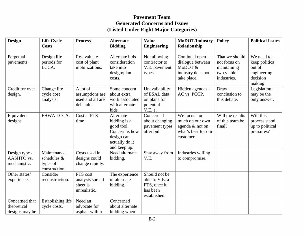
Pavement Team Generated Concerns and Issues

(Listed Under Eight Major Categories)

B-2

Design Life Cycle

Costs Process Alternate

Bidding Value Engineering

MoDOT/Industry Relationship

Policy Political Issues

Perpetual pavements.

Design life periods for LCCA.

Re-evaluate cost of plant mobilizations.

Alternate bids consideration take into design/plan costs.

Not allowing contractor to V.E. pavement types.

Continual open dialogue between MoDOT & industry does not take place.

That we should not focus on maintaining two viable industries.

We need to keep politics out of engineering decision making.

Credit for over design.

Change life cycle cost analysis.

A lot of assumptions are used and all are debatable.

Some concern about extra work associated with alternate bids.

Unavailability of ESAL data on plans for potential V.E.’s.

Hidden agendas - AC vs. PCCP.

Draw conclusion to this debate.

Legislation may be the only answer.

Equivalent designs.

FHWA LCCA. Cost at PTS time.

Alternate bidding is a good tool. Concern is how design can actually do it and keep up.

Concerned about changing pavement types after bid.

We focus too much on our own agenda & not on what’s best for our customer.

Will the results of this team be final?

Will this process stand up to political pressures?

Design type -AASHTO vs. mechanistic.

Maintenance schedules & types of construction.

Costs used in designs could change rapidly.

Need alternate bidding.

Stay away from V.E.

Industries willing to compromise.

Other states’ experience.

Consider reconstruction.

PTS cost analysis spread sheet is unrealistic.

The experience of alternate bidding.

Should not be able to V.E. a PTS, once it has been established.

Concerned that theoretical designs may be

Establishing life cycle costs.

Need an advocate for asphalt within

Concerned about alternate bidding when

Pavement Team Generated Concerns and Issues

(Listed Under Eight Major Categories)

B-3

Design Life Cycle Costs

Process Alternate Bidding

Value Engineering

MoDOT/Industry Relationship

Policy Political Issues

used rather than basing PTS on proven methods.

department. not equivalent thicknesses.

Design methodology selection.

Projected maintenance.

Use pavement management to support process.

Additional designer work involved with alternate bids.

Pavement design & analysis is scattered all over MoDOT.

Time frame original pavements last & time frame overlays last.

There is a need for a survival analysis.

Best choice is alternate bidding.

Thickness of pavements.

Look at percentage of joint repairs after 25 years.

The process will be followed after it’s set.

Subbase options.

Use realistic discount rate.

Existing process flawed.

New AASHTO equations included in PTS or not.

How will pavements perform under new design?

Transparent process.

Unknown about future design performance vs. old designs.

What do taxpayers have at end of design life?

Re-evaluate tons laid per hour on estimating costs.

Overlay the driving surface only.

Value for smoothness over the life of

Material selection for parts of state.

Pavement Team Generated Concerns and Issues

(Listed Under Eight Major Categories)

B-4

Design Life Cycle Costs

Process Alternate Bidding

Value Engineering

MoDOT/Industry Relationship

Policy Political Issues

the pavement. Stage construction.

Evaluate the cost savings of smooth pavements for the traveling public.

All subjective decisions explained & documented.

How can this process keep up with an ever changing industry?

User costs be addressed.

Secret information included in current PTS analysis.

Do we (and if how) include, develop, quantify, calculate, etc. user delay costs?

Need to track maintenance better.

Look at plant site development for portable plants. 95% of time plants are in existing quarry sites.

How do we measure success?

Value for RAP

Pavement Team Generated Concerns and Issues

(Listed Under Eight Major Categories)

B-5

Design Life Cycle Costs

Process Alternate Bidding

Value Engineering

MoDOT/Industry Relationship

Policy Political Issues

at maintenance intervals.

Design recycle in asphalt mixes.

Too many undocumented subjective decisions.

Review of pavement selection at time of selection.

APPENDIX C

Perpetual Hot Mix Asphalt Pavement Design

C-2

Perpetual Pavement Concept

Author: John Donahue, P.E. Date: August 4,2003 A long lasting pavement must successfully endure different failure mechanisms or distresses. Controlling these distresses can theoretically extend the life of the pavement for an indefinite period. This assumption is the underpinning for the perpetual pavement concept. Designing the structure for a perpetual pavement requires the following steps: (1) determining the principal structure-related distresses that must be eliminated, (2) determining the pavement response threshold for each distress below which the pavement can withstand unlimited load repetitions, and (3) selecting the mix designs and layer thicknesses required to keep anticipated pavement responses below the perpetual threshold. The principal structure-related distresses for HMA pavements are fatigue cracking and rutting in the subgrade. The defining pavement response for each is radial tensile strain at the bottom of the HMA layer and vertical strain on top of the subgrade (see figure), respectively. Nonstructural-related distresses, such as thermal cracking, raveling, and HMA rutting, result from poor mix design and construction quality and are considered controllable without structural design modifications. Much research has been performed to determine pavement response thresholds in laboratory environments. Of the two load-related distresses, fatigue cracking usually predominates, especially for thicker HMA pavements where vertical strains on the subgrade are well below the

Repeated Deformation Leads to

Rutting Vertical strain (P.P. threshold ~ 200µε)

Subgrade

Radial tensile strain (P.P. threshold ~ 70µε)

Thick HMA

Repeated Bending Leads to Fatigue Cracking

BBaassee ((aass rreeqquuiirreedd))

C-3

critical threshold, which are typically around 200 microstrains (one microstrain is equivalent to deforming one inch of material by one-millionth of one inch). Lab testing consists of cyclic loading on an end-supported HMA beam supported until failure. Reducing the flexural stress, and subsequently the tensile strain, increases the number of repetitions to failure (defined as the point where the HMA stiffness is half of its original value) until the relationship becomes asymptotic and the repetitions approach infinity. This critical threshold varies with each HMA mix, but the most oft stated value is 70 microstrains. Once the pavement response threshold values are known for a given HMA mix the structural design process begins. Either an elastic layer program (ELP) or finite element model (FEM) is used to determine the layer thicknesses required to generate strains below the perpetual pavement limits. Common characteristics of perpetual pavements are thick combined layers, high stiffness surface layers (to resist mix rutting), and low voids, low stiffness bottom layers. The perpetual pavement concept allows for the fact that some type of surface deterioration (mix rutting, raveling, oxidation, top-down cracking, etc.) will occur within the life cycle design period. Removal and replacement of the surface course would be the expected plan of action. However, the remainder of the structure, if properly designed, should at the very least provide an extended service life.

APPENDIX D

Position Paper

Rock Base

Two-Foot Rock Base Guideline for Rigid and Flexible Pavements Author: Denis Glascock, P.E. Brad Temme, E.I.T. Construction and Materials, MoDOT Date: April 25,2003 MoDOT specifications allow for the use of a two-foot rock base as an alternative to an engineered base system. Sec 303.1 of the Standard Specifications states, “This work shall consist of furnishing and placing select rock excavation material in the top two feet (600 mm) of the subgrade, in conformance with the lines, grades and typical cross sections shown on the plans or established by the engineer, for use as a base to provide pavement support and drainage.” This alternative is also outlined on the Pavement Structure Design Charts used when engineering a suitable pavement for a specific location. These charts state, “All Heavy Duty pavements will be placed on a Stabilized Permeable Base, on 4 inches (100 mm) Type 5 base, with a drainage system. All Medium and Light Duty pavements will be placed on 4 inches (100 mm) Type 5 Base. Rock Base, minimum of 2 feet (600 mm) thick, may be substituted for either base system when available on the job site or economically practical to haul in.” Research for this paper included a review of the standard specifications of Illinois, Kansas, Iowa and California. These states did not give explicit guidelines for the amount of rock base required on any given project. The AASHTO Guide for Design of Pavement Structures yielded the following information:

Minimum Thickness (inches) Traffic, ESAL AC Aggregate Base

less than 50000 1 4 50000 - 150000 2 4

150000 - 500000 2.5 4 500000 - 2000000 3 6 2000000 - 7000000 3.5 6

greater than 7000000 4 6

“Because such minimums depend somewhat on local practices and conditions, individual design agencies may find it desirable to modify the above minimum thicknesses for their own use.” These guidelines are not particularly useful in determining whether MoDOT is currently using the most effective base thicknesses, because they only give a best-case scenario. AASHTO goes on to state that surface treatments will have a dramatic effect on the amount of subbase material that is necessary for a given pavement. “Individual agencies should also establish the effective thicknesses and layer coefficients of both single and double surface treatments. Thickness of the surface treatment has a negligible effect on the structural number (SN) but its effect on the base and subbase properties may be large due to reductions in surface water entry.” The AASHTO analysis left out many design considerations that will affect the performance of the pavement. The AASHTO guide recommends 6 inches of aggregate base on pavements that experience high traffic usage, whereas the MoDOT specification allows for 4inches Type 5 aggregate base. This may indicate that for some projects, MoDOT may not be using an adequate base system.

The Aggregate Handbook provided by the National Stone Association provided data that more closely resembles real world conditions. Table 11.14 of the Aggregate Handbook (attached) shows the total pavement thickness as a function of subgrade soil conditions and traffic intensity. Table 11.13 (attached) gives further explanation on the Traffic Design Indexes used in Table 11.14. MoDOT projects would most likely fall in the higher traffic categories. Table 11.15 (attached) gives detail to the characteristics of the subgrade soil conditions. From Table 11.15 it is apparent that most of the soils encountered on MoDOT projects would put the design in the Fair to Poor range. The worst-case scenario design would call for a 26” total pavement thickness, with a minimum of 4 inches hot-mix asphalt surfacing. MoDOT’s requirement of two feet would exceed the minimum base requirement by 2 inches. Note also, the discussion of railroad track structure where a two-foot ballast and sub ballast is recommended. While a rail car weighs several times that of a typical semi-truck, the rail car is on rails and ties, which intentionally spread the load over a large area. The goal is to have the rail and ties, the “pavement”, move as little as possible under load. Nonpoint Education for Municipal Officials Technical Paper Number 8 written by Jim Gibbons, a UConn Extension Land Use Educator, addresses Pavements and Surface Materials. (attached) Page 2 of this document states, “The Base Coarse might range from 6 to 18 inches depending on the designed use and the bearing strength of the material used. If the material has low bearing strength, subbase thickness is increased or stronger materials used.” This again may suggest that 4 inches of Type 5 aggregate base would not be adequate. It may also suggest that 24 inches of road base may be too much. Addressing the issue that 24 inches may be too much base, can be difficult due to the inability to determine the gradation and quality of the material that is being used for this two-foot rock base. While the literature search yielded few definitive statements about rock base, the assumptions made at the time of the two-foot rock base was established for use under MoDOT pavements are still valid. Those assumptions are:

1. Quarry run or “shot” rock is relatively inexpensive, especially when taken from the jobsite, and is very effective in it’s ability to bridge many existing soil conditions that, otherwise, afford little support for a pavement.

2. Allowing a two-foot thickness decreases the need for additional

processing of the material to eliminate oversized rock, which might protrude above grade. A thinner layer will require additional processing and will encourage the inclusion of more finely graded material, which tend to choke the layer and eliminate some of its functional advantage.

3. Quarry run rock, if properly selected and placed, is a truly drainable material that allows water in the pavement structure to dissipate as quickly as downstream drainage features may allow.

4. Calculations (attached) were computed to determine what thickness of rock would be needed to provide short-term storage of free water, away from traffic, following a period of precipitation. Reducing the thickness of this layer will cause a corresponding reduction in the free water storage capacity of the layer.

5. The two-foot thickness provides adequate support to allow construction

equipment access to the jobsite via the roadbed typically without any damage to the roadbed. This allows the project to progress towards completion faster than an equivalent job on alternate base materials.

6. The two-foot thickness provides significant mass as an integral part of the pavement structure. This “mass” is effective because the large rocks typically used interlock with one another and are isolated from the effects of hydraulic pressures, which are very destructive in other base configurations. This mass offsets, to an extent, the dynamic forces caused by today’s heavy trucks, which are likely to become heavier in the future.

7. It was the hope, intent, and assumption that a two foot rock base would

provide “over design” and would not be the cause of pavement distresses as has often been found in pavements constructed on conventional bases.

There is nearly universal agreement that a good base contributes to the constructability and survivability of a pavement structure. One might argue that a rock base could be less than two feet thick and still be effective. The question is, how thick is enough? As previously mentioned, if the amount of material in the base were reduced, additional controls would on the quality should be employed to reduce the chance that oversized material would create localized “points of support”, to the detriment of the pavement. Gradation limits should be engineered to allow the base to drain properly, and also to provide a stable platform for the pavement. Of course, that might lead one to Type 5 aggregate base. The current two-foot rock base may be using materials that are not the best alternative because the specification is very open with regard to quality of rock. As these various criteria are considered and compared, it becomes apparent that two extremes are currently specified. The four-inch quality controlled and graded material is essentially a working platform that affords very little structure. The two-foot “most anything goes” rock base clearly provides significant structure with minimal quality and gradation control and may, in fact, be over designed in may instances. For publicly owned infrastructure, the conservative approach is superior, especially for facilities that are expected to be in place for generations. Anything invested in the base of a structure, even if over-designed, will yield long-term benefits that are difficult to quantify, but exist, nonetheless.

TAYLOL1

D - 7

TAYLOL1

D - 8

APPENDIX E

Recommendations For

Pavement Bases and Subgrades

E-2

Recommendations for Pavement Bases and Subgrades Author: Pat McDaniel, P.E. Date: May 6, 2003 A technical team of FHWA and MoDOT personnel was formed to address base and subgrade issues generated by the Pavement Team. The technical team consisted of Steve Laffoon and Virgil Stiffler of FHWA and Mike Fritz, Denis Glascock, Jerry Hirtz, Pat McDaniel and Mark Shelton of Construction and Materials, MoDOT. Pavement Team Issue: Recommending to use the Illinois DOT practice to determine when to require subgrade stabilization and as a performance measure in the field for determining if subgrade stabilization requirements have been met. The Illinois DOT practice requires conducting Moisture-Density and California Bearing Ratio (CBR) tests. The CBR of a soil is an indication of the strength of the subgrade material relative to that of crushed rock. Technical Team Response: The team concurs in principle with the recommendation by the Pavement Team. The district soils and geologist technician can take the required soil samples when performing the soil survey for a project, and the Materials Laboratory has the equipment and capability to perform the required tests. But because CBR testing would be difficult to perform in the field when trying to verify if subgrade stabilization has been reached, it is recommended that other test procedures be researched that could be used in lieu of the CBR test, but can be correlated to CBR values. (Action Item: Mike Fritz will try to identify alternative soil tests to CBR that would provide a good correlation to CBR values, but which are more conducive for conducting in the field.) Pavement Team Issue: Consider allowing asphalt pavements to be placed directly on the subgrade with no aggregate base. Technical Team Response: No pavements should be placed directly on the subgrade. An aggregate base is needed to remove water away from beneath the pavement to minimize damage to the pavement and to prevent the subgrade from becoming saturated. Pavement Team Issue: Consider reducing the thickness of the two-foot rock base. Technical Team Response: Specifications should be revised to require all available rock on a project to be placed at the top of fills. Currently, often the practice by contractors is to place rock encountered in the field at the bottom of fills. In regards to the current specified thickness of the two-foot rock base, the thought process used to derive to two feet was felt to be still valid, and therefore should not be reduced on heavier truck trafficked routes. (The position paper on the two-foot rock base provided in Appendix G was submitted to the Pavement Team as supportive data for the technical team’s recommendation.) Based on the original assumptions for the two-foot rock base, the technical team recommends that the thickness of the rock base remain two feet thick at the outer edge of the pavement for heavy and medium duty pavements, but may be reduced for light duty pavements or when a 4-inch drainable base is provided on top of the rock base.

E-3

Pavement Team Issue: Consider alternate base configurations to that currently specified. Technical Team Response: The attached alternate base designs are recommended for bases beneath HMA and PCC pavements. When the CBR for the existing subgrade soils have a CBR value of six or less, stabilized subgrades is recommended for all alternates, except when the rock base is 18 inches or thicker.

Heavy Duty Pavement

4 % Sl ope

Pavement

Rock Base a

4 % Sl ope

Pavement

Type 1 or 5 Base

4” Stabilized Permeable Base

b

4 % Sl ope

Pavement

Rock Base

4” Stabilized Permeable Base

c

Alternate 1

a Shot or Processed Rock

Minimum Thickness 18” at Centerline Rock Base is Daylighted

Max Nom. Agg = ½ Lift Thickness at Centerline

Alternate 2 b

Minimum Thickness 4” at Centerline

Alternate 3 c Shot or Processed Rock

Minimum Thickness 4” at Centerline

Max Nom. Agg = ½ Lift Thickness at Centerline Fines < 10% Earth, Non-Durable Rock

Medium Duty Pavement

2 % Sl ope Pavement

4% Slope

Type 5 Base d

4% Slope

Pavement

Rock Base

2 % Sl ope

e

Alternate 1

d Minimum Thickness 4” at Centerline

Alternate 2 e Shot or Processed Rock

Minimum Thickness 18” at Centerline Rock Base is Daylighted

Max Nom. Agg = ½ Lift Thickness at Centerline Fines < 10% Earth, Non-Durable Rock

E-4

Light Duty Pavement

2 % Sl ope Pavement

Type 1 Base

4% Slope

f

4% Slope

Pavement

Rock Base

2 % Sl ope

g

Alternate 1

f Minimum Thickness 4” at Centerline

Alternate 2 g

Shot or Processed Rock Minimum Thickness 4” at Centerline

Max Nom. Agg = ½ Lift Thickness at Centerline Fines < 10% Earth, Non-Durable Rock

APPENDIX F

PCCP Full Depth Repairs Estimate

F-2

Introduction The estimated percentage of jointed plain concrete pavement (JPCP) surface area that would require full depth repairs at 25 years for LCCA purposes was determined through a combination of different analyses. First, actual past history repair data on construction projects was gathered and normalized to 25 years. Second, mechanistic-empirical (M-E) computer modeling was performed to predict slab deterioration for different thickness JPCPs. Actual Past History Repairs Analysis MoDOT Districts were surveyed for as-built repair work on recent PCCP rehabilitation projects. A total of fifteen projects completed within the past three years were submitted. All pavements were jointed reinforced concrete (JRCP) design, which is no longer used by MoDOT. The total project area was over two million square yards as shown in the table below. JRCP thicknesses ranged from eight to ten inches.

Rte. County Area (yd2) Age Repair % Repair % @ 25 yrs 470 Jackson 321066 23 2.0 2.2 169 Clay 37395 35 2.7 1.9 9 Clay 22401 35 3.6 2.5

210 Clay 35327 30 1.2 1.0 435 Platte/Clay 608840 18 1.2 1.6 67 St. Charles 38720 50 2.1 1.1 100 Franklin 169000 40 1.3 0.8 44 St. Louis City 22213 34 5.6 4.1 64 St. Louis City 47214 36 5.5 3.8 65 Christian/Greene 52800 43 4.6 2.7 60 Stoddard/New Madrid 182250 35 3.1 2.2 55 Ste. Genevieve 211442 30 2.4 2.0 44 Greene/Webster* 88563 29 2.3 2.0 44 Greene* 123879 39 2.6 1.6 44 Greene* 157358 39 2.6 1.7 * resurfacing project

Average % repairs in 25 years for diamond grinding / repair only projects = 1.9

Average % repairs in 25 years for all (including resurfacing) projects = 1.8

It was assumed that the pavements deteriorated linearly over their lifetimes. The linearity assumption is not totally correct, but was a good approximation for the purpose of this analysis. Therefore, based on a linear increase from year 0 to the year of rehabilitation the repair percentage at 25 years was calculated for each pavement. Then the overall

F-3

average repair percentage at 25 years was calculated for the 12 diamond grinding and/or repair-only projects and again for all projects including the three that were resurfaced. The resurfacing projects had little impact on the average percentage. Mechanistic-Empirical Design Analysis The draft version of the new M-E AASHTO Pavement Design Guide program was used to measure the rate of deterioration for JPCP pavements at 25 years. Total traffic was 23 million trucks over the design period, which would convert to above or below 100 million ESALs, depending on the number and weight of axles and simulate a very heavily traveled corridor. Design inputs in the program were those typical of a Missouri JPCP. The results of this analysis are shown in the graph below.

Percent Cracked Slabs in JPCP w/ DG2002Slab Thicknesss

0

10

20

30

40

50

60

70

7 8 9 10 11 12 13 14 15

Slab Thickness (in)

Cra

cked

Sla

bs (%

)

25 years35 years

25-year truck traffic = 23.0 million

35-year truck traffic = 33.7 million

The results indicate that any pavement ≥ 11 inches would incur a negligible number of cracked slabs at 25 years (0.3 percent for 11 inches) and, hence, a negligible number of full depth repairs, although there are other forms of deterioration such as joint spalling that are not addressed here, but which would probably require a lesser degree of repair. This analysis will be revisited in the future after the M-E design model has been calibrated to Missouri pavement conditions, however; it is not anticipated that the results will change drastically from those derived from the national calibration.

F-4

Conclusions The current average repair percentage for rehabilitated PCCPs in Missouri is 1.8 – 1.9. This percentage applies to thinner pavements than are currently being constructed on almost all arterial routes. The improved design features in the current JPCP design (besides greater thickness), such as widened slabs, tied shoulders, and shorter joint spacing, are expected to contribute to better long-term performance and fewer repairs at the time of rehabilitation. The results of the M-E analysis supported this expectation. Based on this information, a policy decision was made to assume for LCCA purposes that full depth repairs in JPCP at 25 years will be 1.5 percent. This number allows a reasonable reduction, in light of the improved PCC design, without setting an unjustified estimate that cannot be verified without further performance data and local calibration of the M-E model. For unbonded PCC overlays, it was decided that the repair percentage for new JPCPs should also be used for these in the interim pavement type selection process. This assumption was deemed necessary, because no rehabilitation data for unbonded PCC overlays in Missouri, of which the oldest is 18 years, is yet available.

APPENDIX G

Subgrade Stabilization Chart

IDOT LOCAL ROADS & STREETS AUGUST - 1995

0

5

10

15

20

25

0 1 2 3 4 5 6 7 8 9

Subgrade CBR

Req

uire

d Th

ickn

ess

Abo

ve S

ubgr

ade,

Inch

es

Remedial Procedures

Optional

Remedial Procedures Required

* Note : Curve is adequate for most construction loadings

Remedial Procedures

Not Required

APPENDIX H

Position Paper on MoDOT’s

Existing Pavement Structure Design

H-2

Rationale for MoDOT’s Current Pavement Structure

Author: Denis Glascock, P.E. G.1 Technical Support Engineer Construction and Materials, MoDOT G.2 Date: January 2003 MoDOT’s history is all about building roads and pavements. “Get Missouri Out of the Mud” was an early slogan of the department and was achieved with the tools and material available at the time, initially, gravel taken from natural deposits and various crushed aggregates. Where traffic justified it and funding was available, “hard surface” roads were provided using Portland cement concrete and various bituminous mixtures. Over the years MoDOT engineers observed the performance of MoDOT’s pavements, conducted formal research, and reviewed the information available from other sources, such as industry, the Federal government, and other state highway agencies. Based on that information, adjustments to pavement design criteria were made. Since the 1920s it was readily accepted that a minimum thickness of Portland cement concrete was required to support even a minor load without immediately cracking. Practical experience with the loads of the day and the materials available established the initial accepted thickness for concrete pavements. Bituminous roadways were usually built up over the years by initially covering an existing dirt or aggregate road and successively adding one layer at a time. Compaction was an on-going process performed by normal traffic, and the road surface was augmented with additional material as necessary to maintain an acceptable riding surface. In the 1960s MoDOT developed thickness charts based on findings from the AASHO Road Test conducted in 1958-60. Two separate empirical methods were created for rigid (PCC) and flexible (HMA) designs. Portland cement concrete (PCC) pavement thickness varied from seven inches to ten inches based on the number of daily equivalent single axle loads (ESALs). The HMA pavement thickness varied from nine inches to 30 inches based on the number of daily ESALs and the soil group index. ESALs were calculated differently for rigid and flexible pavements. The primary factor for the wider variance in flexible pavement design thickness was influence of subgrade support. HMA layers transfer the load more directly onto the subgrade, while PCC is able to bridge areas of poor support. Several iterations of the AASHO Road Test design occurred during the following decades, including the 1986 version, which MoDOT eventually adopted for its current pavement type selection process. A software application, which was developed based on the 1986 version, facilitated multiple design thickness test runs. The design recommendations generated by the program were considered acceptable because they reflected MoDOT’s experience with pavements and they assured consistency from one situation to the next. In 1990 MoDOT’s Chief Engineer visited Europe to examine their pavements and pavement design processes. Upon his return he directed MoDOT to design and build better pavements. Work on this assignment was initiated at that time, considering both the European process

H-3

information, and the wealth of data that was available specific to pavement types in Missouri. It was stated that the criteria for the “new” design would include a review of the things that Missouri had done through the years, what had gone wrong or right with existing pavements, and whatever might be applicable from current practice around the world. The effort consumed several years as the available information was considered and consolidated into a final design. The new pavement design was adopted by MoDOT in 1993. Critical issues addressed in the new design process included the following:

1. The value of drainage cannot be overestimated. 2. A pavement should not be allowed to fail due to loading. 3. Equivalent designs of HMA and PCC pavements must be established. 4. A paved shoulder is an integral part of the pavement structure. 5. Simple is better. 6. Design out the known construction and maintenance issues. For example:

• Dissimilar materials – PC pavement next to AC shoulder • High steel • Mid-panel cracking • Rutting

7. Account for the limitations placed on MoDOT’s maintenance forces.

Concurrent with the process of selecting the desired general pavement characteristics, the parameters of thickness were established using repeated iterations of the AASHTO pavement design program (DARWin). A sensitivity analysis of the design variables was conducted, as was an effort to quantify MoDOT’s ability to determine an appropriate value for each variable. The assumptions shown in Table 1 were made. Each HMA pavement thickness, as determined by the equations, was rounded to the nearest 0.25 inches. Portland cement concrete pavement thickness was rounded up to the next full inch. The tables were intended to “break” at significant ESAL counts, and for HMA pavements, significant variations in soil support characteristics. It was also assumed that MoDOT is experiencing an increase in the number of undocumented “super loads”, loads that significantly exceed the design capacities of bridges and pavements. The tables were intentionally designed conservatively to account for those super loads, and for variations in construction quality as might not be caught by the inspection process. In 1993, the AASHTO Design Guide was revised yet again and the software was upgraded accordingly. MoDOT’s current pavement design criteria are intended to provide a reliable pavement structure in spite of any variation that may be introduced to the system. The negative effects attributed to environment, contractors, construction equipment, maintenance procedures and the pavement users have been taken under consideration. Failures due to under-design are not anticipated.

H-4

Table 1. 1993 Pavement Design Assumptions H Issue HMA Pavements PCC Pavements Analysis Period 35 years 35 years Discount Rate 4.0 4.0 Number Lanes, one direction 2 2 Lane Width 12 12 Combined Width, lane + shoulder 22 22 Soil: Very Poor 2515 * Poor 3685 Moderate 4955 Good 7300 Level of reliability 90% 90% Design Terminal Serviceability 2.5 2.5 Consider swelling/frost heave N N Performance initial period 35 years ** 35 years Service Index – initial 4.5 4.5 Traffic: Growth 2.1 2.1 Compound growth C C Initial ESALs *** *** Directional Distribution 100 100 Lane Distribution 100 100 Standard Deviation 0.4 0.4 HMA Pavement Layers

Lift Thickness Coefficient. Modulus Drainage Top Lift 1.25 0.44 450,000 1 Second Lift 1.75 0.43 425,000 1 Bituminous Base Varies 0.42 400,000 1 Aggregate Base 4.00 0.07 15,000 1

PCC Pavement Layers Lift Thickness Modulus Drainage Base 4.00 15,000 1 Pavement Varies **** 3,605,000 1 Load Transfer was set to 2.8 as all pavements were to have tied shoulders (> 2’), or the pavement would be made one inch thicker to compensate. Loss of support was set to zero.

* Very Poor modulus of subgrade reaction was used for all PCC pavement structures because there was no intent to break up the results by soil modulus, and soil modulus had no effect on the structure of PCC. ** It was never expected that the surface layer would weather for this period of time. The intent was to indicate to the equation that we wanted to place the entire structure at the time the original pavement was constructed. The final criteria stated that the surface lift would be replaced after 15 and 25 years.

H-5

*** Initial Traffic varies as necessary to result in desired total ESALs. A typical growth rate is assumed to account for anticipated compounded growth of traffic on the section. Distribution is not an issue as the calculations determine total ESALs accumulated on the design lane. **** Engineering judgment said to restrict this to a minimum of 8” in all circumstances.

APPENDIX I

MoDOT Pavement Design Methodology

I - 2

MoDOT Pavement Design Methodology Author: John Donahue, P.E. Date: July 31,2003 How does MoDOT design pavements for the State highway system? Pavements on the Missouri highway system have long been designed using the contemporary theory and rationale prevalent in each era of the 20th century. Missouri never strayed far from the designs used by other States nationally or at least regionally. Changes to design have come incrementally as better understanding of pavement performance under various conditions became known. Since the 1920s States either alone or in joint efforts have constructed, monitored, and analyzed new design features in pavements. Examples of these trial-and-error efforts were the experiments with contraction and expansion joints and transverse joint load transfer devices in the late 1930s and 1940s, in which Missouri played a lead role. By the end of the 1940s the conclusion was reached that expansion joints, except in unique circumstances, were not necessary in PCC pavements and that, in fact, they reduced the overall load transfer ability of the pavement joints. At the same time, the necessity of dowel bars at transverse joints for load transfer became fairly institutionalized. Currently, MoDOT uses the empirical American Association of State and Transportation Highway Officials (AASHTO) design method that most other States are also using. Explain the current AASHTO design method? The current method is derived from a comprehensive pavement study, the American Association of State Highway Officials (AASHO) Road Test, conducted in the late 1950s and early 1960s in Ottawa, Illinois along the alignment of what would become I-80. The primary objective of the study was to establish relationships showing how performance was affected by structural design and loading. Pavement test sections were constructed, with a few exceptions, using typical designs of that day. Portland cement concrete (PCC) or rigid pavements were 5 to 12.5 inches thick on variable thickness sand-gravel bases, while hot mix asphalt (HMA) pavements were up to 6 inches thick on variable type (cement-treated, asphalt-treated, and gravel) and thickness bases on variable thickness sand-gravel subbases. Material and construction quality was tightly governed to ensure homogeneity within the test sections. Single- and tandem-axle trucks loaded from 2,000 to 48,000 pounds per axle circled around 2,000- to 6,800-foot long loops over a two-year period. Performance data was collected from exhaustive distress surveys and instrumentation testing.

I - 3

The end result of this extensive program was the creation of pavement thickness selection charts and formulas for different load levels. The number of load levels defined a design life, since one could estimate the truck traffic over a given period of time. The basis for the pavement thickness – load relationships was derived from the change in ‘serviceability’ index, which was a subjective ‘seat-of-the-pants’ 0 – 5 point rating scale for ride quality. Serviceability indices were translated into a combination of objectively measured pavement distresses: slope variance (profile), cracking and patching, and rut depth for HMA pavements; slope variance and cracking and patching for PCC pavements. The design life of the pavement was based on the change in serviceability index from initial construction (4.2 – 4.5) to a level where ride became unacceptable (2.0 – 3.0). To simplify, for a given pavement structure an engineer could estimate the number of trucks it would require to reach a state of measurable distress that equated to unacceptable ride quality. Over the years the original design methods have been tweaked and enhanced to consider previously overlooked variables, such as drainage, subgrade support, and construction reliability, or changing design configuration, such as tied shoulders for PCC pavements. These methods have been extended far beyond their original limits. Over four-fifths of the States use a version descended from the original AASHTO empirical design method. Not all States use the most current one; some are still basing designs on the 1972 version. Missouri’s current structural design thicknesses for new HMA and PCC pavements were generated from the 1986 version. The last overall major revision to the empirical AASHTO design method occurred in 1993. Supplementary revisions to the rigid pavement design were published in 1997. What exactly is an ‘empirical’ design? All of these past studies could be considered part of the continuing empirical process, which has formed the basis for the size, shape, and design of nearly every significant pavement. Empirical design methods are based on observations of performance of pavements with known dimensions and materials under specific climatic, geologic, and traffic conditions. This method is

AASHO Road Test Layout in Ottawa,

I - 4

predominantly beneficial to States that can duplicate the conditions inherent in the development of original empirical design. Naturally the State that could reap the most benefit from an empirical design would be the one that built the pavements used to develop it. On the other hand, another State, far removed from the first State’s geologic and climatic conditions, would have to make assumptions about the suitability of applying that empirical method to their design. This was the problem with the AASHO Road Test in the 1950s. The Illinois location was selected because its conditions supposedly represented a broad cross-section of the country, however; the Road Test Special Report cautioned engineers that ‘findings of the research relate specifically to the soils and the materials actually used in the test pavements, to the conditions under which the materials were placed, and to the environment and climate of the test site’. The test site might have been representative of the region, including Missouri to an extent, but it was still vastly different from areas such as the arid desert climate of the southwest. The authors of the study did assume that ‘sound engineering judgment has been used successfully to apply knowledge attained from limited research to problems over wider areas, and presumably similar applications can be made with the knowledge obtained from the Road Test’. In other words, it was up to the other States to figure out how to wisely adapt the findings to their pavement designs. Prediction models for serviceability must be modified through additional testing and verification. An attempt was made to do this with AASHO Test Road satellite test sections constructed and monitored by different States in the 1960s and 70s, but the effort had inconsistent support, with only a handful of States (Missouri among them) providing more than a token commitment to the program, and fell far short of original expectations. Provide a simple example of an empirical design. A good way to illustrate the benefits and drawbacks of an empirical design would be to examine the following hypothetical case. Missouri decides to build a 13-inch asphalt concrete (HMA) pavement on a 4-inch crushed stone base on a silty-clayey soil with a high water table and poor drainability. Within the same year Missouri builds another pavement having similar features, except with a 10-inch HMA thickness, in an adjacent county. Climatic conditions and truck traffic projections are nearly the same for the pair. A long-term performance study is conducted for the two pavements. The study of the 10-inch HMA pavement concludes at a certain point in time when it reaches a critical stage where rehabilitation is required. Several years later the same thing happens to the 13-inch pavement. Based on the results of the study, design life predictions are developed for HMA pavements with granular bases on fine-grained soils under similar traffic conditions. The design lives are interpolated for HMA pavements between 10 and 13 inches thick. Extrapolation is used to predict design lives for 8- to 9-inch and 14- to 15-inch HMA pavements. It is evident that this prediction model is fine for HMA pavements meeting the narrow criteria of this road test for soils, climate, traffic, and even mix design, but it would have limited use for pavements outside these ranges.

I - 5

Perhaps a simpler way to explain the empirical method is to use an archery analogy. An archer could learn to very closely estimate the distance of his arrow’s flight through trial and error. Drawing back the string the same distance on the same bow for the same type arrow every time he could mentally catalogue the landing points for a variety of release angles. With good approximation he could estimate the distance for angles he never tried. For example, knowing the exact distances the arrow flies at 40° and 45°, he could interpolate between those points and know the general location an arrow shot at 42° would land. Were he to use a different weight arrow he would have to start the empirical process over since the landing spots would change. Likewise, pulling the string back further on the bow would change the results. The archer could go through a complex series of tests using different size and weight arrows at different pulls at different angles to develop a full mastery of controlling the arrow’s flight distance, assuming other variables not heretofore mentioned, such as wind speed,

13” HMA Test Section

10” HMA Test Section

Known performance prediction

Interpolated performance prediction

Extrapolated performance prediction

11” – 12” HMA

14” – 15” HMA

8” – 9” HMA Extrapolated

performance prediction

Known performance prediction

Empirical Design Example for HMA

I - 6

elevation, etc., remain constant (and assuming the archer has a remarkable memory). But, it would only pertain to the bow he’s using. The archer then would have gone through a thorough empirical process that yielded very reliable results within the variable constraints mentioned above, but he would have gained absolutely no knowledge of the physics controlling his arrow’s flight. If he had known Newton’s Second Law of Motion (Force = Mass x Acceleration), he would have understood how the bowstring’s tension and the earth’s gravity affected the arrow’s trajectory and been able to predict it without going through an elaborate testing process. Although the predicted results would have been nearly the same, in essence, he would have converted from an empirical to a ‘mechanistic’ method of determination.

‘Mechanistic’? This mechanistic method, using simple physics, would have allowed incredible flexibility under different circumstances. Not only could he predict flight distances for bow variables such as pull tension, angle, and arrow mass, but he could also account for external variables, including elevation and wind speed. Of course, he would be wise to validate theoretical results with some field tests, but to a much lesser degree than the rigorous empirical process. Going back to our HMA pavement example we can also try to understand the performance results in a mechanistic light. A pavement is a physical object that must respond to the forces acting on it, as an arrow must respond to its applied forces. The pavement will experience specific stresses, strains, and deflections depending on its internal properties (i.e. thickness, modulus of elasticity, etc.) and external influences (i.e. load weight and location, temperature, etc.). In a clean theoretical environment these pavement responses can be accurately predicted. In reality, complex circumstances make pavement response predictions less accurate, but still within reasonable ranges. The problem here is that we’re ultimately interested in pavement performance not pavement response. We need to understand not only how a pavement reacts, but how the reactions lead to deterioration. Unfortunately, mechanistic methods by themselves cannot really predict pavement deterioration. Rather, distress survey data from sample pavements of the variety being modeled must be gathered in order to make the connection from pavement response to performance through what is usually called a transfer function. So unlike determining an arrow’s flight, which is a pure mechanistic exercise, predicting pavement deterioration requires a combination of mechanistic and empirical methods, or more simply, a mechanistic-empirical (M-E) model.

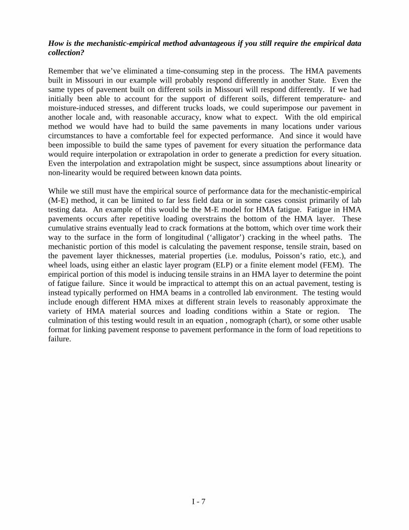
I - 7

How is the mechanistic-empirical method advantageous if you still require the empirical data collection? Remember that we’ve eliminated a time-consuming step in the process. The HMA pavements built in Missouri in our example will probably respond differently in another State. Even the same types of pavement built on different soils in Missouri will respond differently. If we had initially been able to account for the support of different soils, different temperature- and moisture-induced stresses, and different trucks loads, we could superimpose our pavement in another locale and, with reasonable accuracy, know what to expect. With the old empirical method we would have had to build the same pavements in many locations under various circumstances to have a comfortable feel for expected performance. And since it would have been impossible to build the same types of pavement for every situation the performance data would require interpolation or extrapolation in order to generate a prediction for every situation. Even the interpolation and extrapolation might be suspect, since assumptions about linearity or non-linearity would be required between known data points. While we still must have the empirical source of performance data for the mechanistic-empirical (M-E) method, it can be limited to far less field data or in some cases consist primarily of lab testing data. An example of this would be the M-E model for HMA fatigue. Fatigue in HMA pavements occurs after repetitive loading overstrains the bottom of the HMA layer. These cumulative strains eventually lead to crack formations at the bottom, which over time work their way to the surface in the form of longitudinal (‘alligator’) cracking in the wheel paths. The mechanistic portion of this model is calculating the pavement response, tensile strain, based on the pavement layer thicknesses, material properties (i.e. modulus, Poisson’s ratio, etc.), and wheel loads, using either an elastic layer program (ELP) or a finite element model (FEM). The empirical portion of this model is inducing tensile strains in an HMA layer to determine the point of fatigue failure. Since it would be impractical to attempt this on an actual pavement, testing is instead typically performed on HMA beams in a controlled lab environment. The testing would include enough different HMA mixes at different strain levels to reasonably approximate the variety of HMA material sources and loading conditions within a State or region. The culmination of this testing would result in an equation , nomograph (chart), or some other usable format for linking pavement response to pavement performance in the form of load repetitions to failure.

I - 8

Are any other States already using an M-E model for pavement design? Yes, about half a dozen States currently have some form of M-E model for their HMA and/or PCC pavements. The States that don’t have an M-E model for both usually fall back on the AASHTO empirical model for the pavement type lacking an M-E model. Illinois has had an M-E model for both types since the early 1990s. Their HMA M-E model uses the FEM program, ILLIPAVE, to predict fatigue cracking. Although there are mechanistic models for other HMA pavement distresses, such as subgrade rutting, IDOT did not incorporate them because they determined that fatigue was the controlling factor, since the thick HMA layers they were typically designing precluded other load-induced distresses from occurring. The PCC M-E model uses the FEM program, ILLI-SLAB, to predict slab cracking, which IDOT considers the primary failure criterion, overshadowing other load-induced distresses, for their jointed plain concrete pavement (JPCP) designs. Why wasn’t there an AASHTO effort to create a national M-E model for all States? The use of mechanistic methods for pavement design dates back to the 1930s. Researchers working on the AASHO Road Test were well aware of mechanistic principles, and even conducted extensive measurements of pavement stresses, strains, and deflections at the site. A.C. Benkelman used his now famous beam test to try to develop a link between flexible pavement deflections and performance. W. R. Hudson had success correlating rigid pavement edge stresses to fatigue distress. Despite these forays into the beginnings of M-E designs, the models were not fully developed or understood at the time to be widely accepted by all the

Material, Traffic, and Climate Inputs

Pavement Design Period

Pavement Response Prediction

‘Mechanistic’ Analysis

Pavement Distress

Prediction ‘Empirical’

Analysis

Acceptable

Not Acceptable

Mechanistic – Empirical Pavement Design

I - 9

States. These mechanistic experiments were more of a sideshow at the Road Test, overshadowed by the large-scale empirical process taking place. Another hindrance to their development, even had the mechanistic models been fully developed, was the lack of advanced computer technology to process the complex programming in a reasonable time frame for multiple design runs. Although mechanistic outputs could be simplified to catalogue designs for specific pavement types, in order to be useful to all the States the models would have to be run using unique inputs for traffic, climate, soils, and mix material properties, and the computational speed required was decades away from becoming a mainstream reality. That was in the past, why isn’t something being done now? There is something being done. Several years ago AASHTO, through the National Cooperative Highway Research Program (NCHRP), contracted out work to a consultant for the development of a comprehensive M-E program that all States could benefit from. The program is on the cusp of completion. It is being called the 2002 Pavement Design Guide (DG2002), even though we are somewhat beyond the year of its intended completion. The DG2002 program consists of separate modules for HMA and PCC pavements. In addition to analyzing new pavements the program includes different rehabilitation strategies, such as unbonded PCC overlays on old PCC pavements, PCC whitetopping on HMA pavements, HMA overlays on rubblized PCC pavements, and conventional HMA overlays on HMA and PCC pavements. Three major categories of data input are required to run the model: climate, traffic, and materials. Climate is modeled using the embedded Enhanced Integrated Climatic Model (EICM), which predicts moisture and temperature profiles in a pavement profile throughout its design period on an hourly basis using actual weather station data as is or interpolated data between stations for a project location. Loads are modeled using truck traffic data, which the user provides to the level of detail that is possible. Truck data, if available, can be input for every single truck with every type of axle configuration under every load range for every hour of the year, otherwise the user can provide as little as the average annual daily truck (AADT) traffic and use default values for everything else. Material data also has varying levels of user input complexity. Basic level information for layer types and thicknesses is required, but default values for material properties, such as strength-, stiffness-, and gradation-related attributes, are available if the user cannot be more specific. The program takes the three categories of information and processes them through FEM-based analysis to determine pavement responses throughout the design period specified by the user. This activity comprises the ‘mechanistic’ portion of the analysis. These pavement responses are then run through transfer functions to predict the incremental and cumulative level of each distress type pertinent to the pavement being analyzed. This activity comprises the ‘empirical’ portion of the analysis.

I - 10

Will MoDOT use the new AASHTO M-E Design Program? MoDOT fully intends to adopt the DG2002 program for future pavement design analysis, although this decision was not hastily made. Much thought and effort went into evaluating the possibilities of adopting other existing M-E models; however, several factors weighed in against doing so. First, none of the other models had common analysis platforms for climate and traffic for all pavement types. Nor did they integrate this data to the level of detail (i.e. hourly temperature profiles, individual truck axle load spectra, etc.) as the DG2002 program. Providing detailed weather and truck traffic data for one design and using annual averages for the other seemed unequal. Second, the distress models were calibrated using data from the Long Term Pavement Performance (LTPP) program, which provided the largest database of performance and inventory information ever available for contemporary designs. Finally, using an AASHTO-sponsored program provided a defensible platform for pavement design on Missouri’s roads. There would be less appearance of bias for type selection and the analysis procedures would have to be considered mainstream. The DG2002 program will be in final form after it is approved by the AASHTO Joint Task Force on Pavements and receives review comments from State members. Once in final form, the product will be balloted among all States, and, if successful, become an official AASHTO product. Will the new program result in different pavement designs? Pavement designs are limited by the few affordable natural resources available to build them, therefore it will probably not impact our current design types. It might; however, have an impact on pavement layer thicknesses. Outputs that recommend thicker or thinner structural layers will be judged carefully using past experience and risk assessment. Early indications are that outputs from the DG2002 might result in reduced structural thicknesses at higher load levels than the empirical model would have recommended. In the future, the DG2002 will allow us to keep pace with advancements in pavement material technology since the mechanistic engine in the program should be able to predict the new pavement responses associated with these changes. How soon will MoDOT implement the new program? The DG2002 program is not officially available, but should be released for general use by 2004. MoDOT staff have already been privileged to try out beta versions of the software, which were not fully operational, but still provided useful experience with an M-E model and a feel for some of the performance predictions for typical Missouri pavements. When the debugged version is available MoDOT shall begin a complete distress model calibration and sensitivity analysis using various ranges of inputs that are native to Missouri. Eventually, cataloging of typical pavement designs will be produced for general use by MoDOT roadway designers and consultants. A complete transition from the old empirical AASHTO design to the DG2002 should occur by 2005, although project plans developed in 2004 may already incorporate the new designs. Meanwhile the distress models will be calibrated using Missouri performance data to the extent possible on an ongoing basis, thereby ensuring the design predictions match the reality of pavement performance.

I - 11

2003

• Adopt DG2002 model

• Perform sensitivity analysis

• Calibrate distress models

2004

• Continue calibration• Develop catalogue

designs • Update Project

Development Manual (PDM) pavement chapter

• Start incorporating DG2002 designs in project plans

2005

• All project plans for pavements incorporate DG2002 designs

• Continue distress model calibration

DG2002 Implementation Time Frame

APPENDIX J

Critique on Coefficients For

Hot Mix Asphalt Fatigue Distress Model

J - 2

Critique of Using Indirect Tensile Strength Test Results to Determine Fatigue Distress Model Coefficients for MoDOT HMA Mixes

BACKGROUND Traditional fatigue distress models for hot-mix asphalt (HMA) pavements relate the number of load repetitions to failure (Nf), normally defined as the point of halving the original HMA modulus of elasticity or stiffness, to the tensile strain induced at the bottom of the HMA layer by the load. The inverse of the strain (1/ε) is raised to a power coefficient (n) and multiplied by a linear coefficient or shift factor (K) as shown in the following equation.

Nf = K (1/ε)n The n-coefficient has a significantly greater influence on fatigue life, and subsequently HMA thickness, than the K-coefficient, therefore determining a realistic value for the former variable is much more critical. Since the two coefficients are mix dependent, they can be determined through performance tests, traditionally with a beam fatigue device. However, since this type of equipment is expensive and not readily available to all highway agencies, an alternate ‘poor man’s’ method using indirect tensile strength (σIT) tests with Marshall compacted HMA pucks was developed at the University of Illinois in Champaign-Urbana in the 1970s by Maupin and Freeman. The asphalt cements used in the study had a penetration grade range from 62 to 196. Their corresponding mix tensile strengths ranged from 160 psi to 71 psi. Therefore, indirect tensile strength increased with decreasing penetration grade. The following equations show the relationships derived from the study:

n = 0.0374 (σIT) – 0.744

log K = 7.92 – 0.122 (σIT) This method was applied to MoDOT mixes. Since our mixes are currently designed using Superpave procedures, which incorporate the gyratory compactor, Marshall-size pucks were cored out of the larger gyratory pucks and put through the indirect tensile test (ITT). In addition to determining the coefficients, the tensile strain used in the fatigue distress model for each HMA thickness was generated using the finite element program (FEM) ILLI-PAVE. ILLI-PAVE is an iterative flexible pavement analysis tool that models HMA as an elastic material. Nonlinear, stress-dependent resilient modulus material models and failure criteria for granular materials and fine-grained soils are incorporated into the model. Granular materials are considered stress-hardening (modulus increases as bulk stress increases) and fine-grained soils are stress-softening (modulus decreases as deviator stress increases). Principal stresses in the granular material and fine-grained soil layers are modified at the end of each iteration so that they do not exceed their shear strength as defined by the Mohr-Coulomb theory of failure. RESULTS

J - 3

Indirect tensile test results from design mix samples, submitted in the summer of 2003 by various contractors, yielded strengths ranging from from 173 psi to 356 psi, which were well beyond the range used to develop the Maupin-Freeman equation. The power coefficients for these mixes, derived from the Maupin-Freeman equation, ranged from 5.73 to 12.57 with an average of 8.50. The impact these coefficients have on fatigue lives are illustrated in the following graph. Based on an average n-value of 8.50, a 6-inch HMA layer would provide 100,000,000 load (9000 lb) repetitions till fatigue failure, while a 5-inch HMA layer would be more than sufficient for 10,000,000 repetitions. Thicker HMA layers would allow stratospheric load numbers.

Design Life Repetitions vs. n-power CoefficientsLoad = 9024 (lb) / HMA Modulus = 450 (ksi) [Maupin-Freeman n - ITT relationship]

1.00E+04

1.00E+05

1.00E+06

1.00E+07

1.00E+08

1.00E+09

1.00E+10

1.00E+11

1.00E+12

1.00E+13

1.00E+14

1.00E+15

1.00E+16

1.00E+17

3.0 3.5 4.0 4.5 5.0 5.5 6.0 6.5 7.0 7.5 8.0 8.5 9.0 9.5 10.0 10.5

n-power Coefficient

Load

Rep

etiti

ons

6"7"8"9"10"11"12"13"14"15"16"17"

Since these design thicknesses were not realistic based on previous field engineering experience, which might have been at least partly the product of extrapolating the Maupin-Freeman model far beyond its developmental range, MoDOT staff decided that alternate means of predicting these coefficients must be used. Until MoDOT can obtain test results from another mix performance test, such as the beam fatigue device, becomes available, MoDOT will probably rely on national default values in the DG2002 program for the distress model coefficients. Later, these values will be calibrated to Missouri conditions as better mix and field performance data is gathered.

APPENDIX K

Design Estimators’

Cost Analysis Spreadsheets

The following is the Estimators Spreadsheet on Batch Plant Concrete.This page is a summary sheet of inputs and the remaining pages are the actual spreadsheet.

Batch Plant Concrete Spreadsheet

Summary SheetCell D5-D6 enter county and route of project

D11 enter pavement type

D15 enter 0 if non-reinforced, 1 if reinforced

D16 enter project length in miles used for transverse joint sawing and dowel bar quantities.

D17 enter average pavement width, used for transverse joint sawing and dowel bar quantities

D18 enter total longitudinal feet to be sawed, used for sawing and tie bar quantity

D19 enter transverse joint spacing, used for sawing and dowel bar quantities

D20 enter total square yards of concrete from plans

D21 enter concrete thickness

D24 enter county number

D25 enter miles from the cement supplier location

D26 enter mileage from rock supplier

D27 enter mileage from sand supplier

D29 enter cost of cement from supplier, obtain delivered price when possible add 6% tax on material only

D30 enter cost of paving stone per ton at the quarry, obtain delivered price when possible add 6% tax on material only

D31 enter cost of sand per ton from the sand plant, obtain delivered price when possible add 6% tax on material only

K58 enter production rate for project. Production rates for PDM 4-03.16 may be a source.

Haul rates from 1993 PS&E rates adjusted for inflation and fuel prices. Trucking companies and backfiguring haul quotes verify hauling rates.

Equipment Crew from past MoDOT projects. Equipment rates from Rental Rate Blue Book montly rates divided by 175 hrsand Blue Book operating costs. Plant equipment rates are currently under review with Primedia, publisher of BlueBook, assistance.

Labor Rates from Federal and State wage rates.

56789101112131415161718192021222324252627282930313233343536373839404142434445464748495051525354555657585960616263

D E F G I J K L M N O PCounty, RouteMoDOT '03 Letting**THIS SPREADSHEET SHOULD ONLY BE USED ON PROJECTS WHERE PORTABLE PLANTS WILL BE USED**

DIRECTIONS: CHANGE CELLS THAT ARE SHADED TO COMPUTE A NEW ESTIMATE14" Concrete Pavement 15' Joints

Estimate Is Based O 1.0% Profit and Overhead

0 Enter A One If Pavement Is Reinforced0.987 Project Length (Miles)48.1 Pavement Width (AVG.)

10,427.260 Longitudinal Feet To Be Sawed15 Transverse Joint Spacing

28,094.9 Square Yards Of Concrete14.0 Concrete Depth (Inches)

10,926 Cubic Yards Of Concrete

48 County: Jackson10 Estimated Miles From Cement Kiln Or Wholesale Point To Project Midpoint10 Estimated Miles From Source Of Paving Stone To Project Midpoint10 Estimated Miles From Source Of Sand To Project Midpoint

$87.63 Cement Cost Per Ton At Kiln Or Wholesale Point* Cement Supplier$7.44 Cost Of Paving Stone Per Ton At The Quarry* Quarry$3.72 Cost Of Sand Per Ton At The Quarry* Sand Plant

3,264 Estimated Tons Of Cement Required11,929 Estimated Tons Of Aggregate Required6,752 Estimated Tons Of Sand Required

$2.67 Transportation Cost Per Ton For Cement$2.67 Transportation Cost Per Ton For Stone$2.67 Transportation Cost Per Ton For Sand

* Material Quantities Increased By 3% To Compensate For Waste-------------------------------------------------------

SUMMARY OF COSTS

$45,142.89 Paving Equipment Cost$51,403.93 Paving Labor Costs$20,357.65 Longitudinal & Transverse Saw Cuts

$105,961.68 Set Up Costs (Includes Labor + Materials)$294,690.67 Cost Of Cement In Mix (Includes Transportation)$120,576.13 Cost Of Stone In Mix (Includes Transportation)$43,132.68 Cost Of Sand In Mix (Includes Transportation)

$0.00 Cost Of Reinforcing Steel Mesh ($2.50 Per Sq Yd)$2,714.25 Cost Of Reinforcing Rods (Longitudinal Joint) $50.00 per hundredwt.

$5.00 dowel assemblies per ft.$683,979.86 Total Cost Of Concrete

$24.35 Cost Per Square Yard 3,000 ASSUMED PRODUCTION RATE$0.24 Profit and Overhead (S.Y. per day)

------------$24.59 Total Cost Per Square Yard $29.41 Total Cost Per Square Meter

NOTE- DOES NOT INCL. COST FOR BATCH SETUP(ADD TO MOBILZ.)-------------------------------------------------------

6789101112131415161718192021222324252627282930313233343536373839404142434445464748495051525354555657585960616263646566676869707172737475767778798081828384858687888990919293949596979899100101102103104105106107108109110111112113114115116117118119120121122123124125126127128129130131132133134135136137138

B C D E F G H I J K L M N O P

PSC Rates : Effective - 10/29/93 --------------------------------------------------------------------------* Adjusted for fuel increase

EQUIPMENT PRODUCTION AND RENTAL RATES(Rates Obtained From Blue Book or Means)

Min Curr Max AvePer Rate Per Per 8.00 Hr Day

Miles Trip 15% Trip Trip----- ---- ---- ---- ---- Prod. Prod.

1 0.93 1.20 1.04 1.06 Hourly Rate/ Rate/2 1.06 1.36 1.18 1.20 Rental Hour Day3 1.19 1.53 1.33 1.35 Rate (S.Y.) (S.Y.) Number4 1.32 1.70 1.48 1.50 ------ ----- ----- -------5 1.44 1.85 1.61 1.63 133.00 375.00 3,000 1 Batching and Mixing Plant6 1.57 2.02 1.76 1.78 156.50 375.00 3,000 1 Belt Placers7 1.70 2.19 1.90 1.93 160.17 375.00 3,000 1 Slip Form Paving (Surface)8 1.82 2.35 2.04 2.07 43.20 375.00 3,000 1 Water Truck and 2 Work Brid9 1.95 2.51 2.18 2.21 36.07 375.00 3,000 1 Texture Cure Machine

10 2.07 2.67 2.32 2.35 14.58 75.00 600 3 Saw Machines11 2.19 2.82 2.45 2.49 73.61 375.00 3,000 1 Batch Plant Loader Cat 972G12 2.30 2.97 2.58 2.62 74.92 Equipment Hours Required13 2.41 3.11 2.70 2.74 602.55 Hourly Equipment Rate14 2.51 3.23 2.81 2.85 45,142.89 Total Equipment Rental15 2.63 3.39 2.95 2.99 1.61 Equipment Rental Per Square Yard16 2.72 3.51 3.05 3.09 --------------------------------------------------------------------------17 2.82 3.63 3.16 3.2018 2.91 3.75 3.26 3.3119 3.01 3.88 3.37 3.42 --------------------------------------------------------------------------20 3.08 3.97 3.45 3.50 LABOR COSTS21 3.16 4.07 3.54 3.5922 3.23 4.16 3.62 3.6723 3.32 4.28 3.72 3.77 Hourly24 3.39 4.37 3.80 3.85 Rate25 3.47 4.52 3.93 3.97 ------26 3.55 4.68 4.07 4.10 32.76 65.52 11 2 Batch Machine Operator/Loa27 3.64 4.84 4.21 4.23 28.70 28.70 11 1 Batch Plant Laborer28 3.75 5.00 4.35 4.37 32.76 32.76 11 1 Belt Placer Operator29 3.86 5.16 4.49 4.50 32.76 32.76 11 1 Paving Machine Operator30 3.97 5.32 4.63 4.64 32.76 32.76 11 1 Tube Machine Operator31 4.08 5.49 4.77 4.78 32.76 32.76 11 1 Texture Machine Operator32 4.19 5.65 4.91 4.92 28.70 114.80 11 4 Concrete Finishers33 4.30 5.80 5.04 5.05 28.70 258.30 11 14 Laborers34 4.41 5.96 5.18 5.18 32.76 32.76 11 1 Teamster35 4.52 6.12 5.32 5.32 25.00 25.00 11 1 Foreman36 4.63 6.28 5.46 5.46 30.00 30.00 11 1 Superintendent37 4.75 6.44 5.60 5.60 28.70 686.12 11 8 Set Up Team38 4.85 6.60 5.74 5.73 32.76 11 3 Saw Machine Operators39 4.97 6.76 5.88 5.8740 5.07 6.92 6.02 6.00 51,403.93 Total Labor Costs For Paving41 5.19 7.08 6.16 6.1442 5.30 7.25 6.30 6.28 1.83 Total Labor Cost Per Square Yard43 5.41 7.41 6.44 6.42 --------------------------------------------------------------------------44 5.52 7.57 6.58 6.5645 5.63 7.72 6.71 6.6946 5.74 7.88 6.85 6.82 -----------------------------------------------------------------------47 5.85 8.04 6.99 6.96 COST FOR SAW CUTS48 5.96 8.20 7.13 7.1049 6.07 8.36 7.27 7.2350 6.18 8.52 7.41 7.3751 6.29 8.68 7.55 7.51 23.20 Hourly Rental Rate + Operating Costs52 6.40 8.84 7.69 7.64 75.00 Production Rate Per Hour (Lin Ft Per Hour)53 6.51 8.99 7.82 7.77 10,427.26 Longitudinal Feet To Be Sawed (Includes Climbing Lane)54 6.62 9.15 7.96 7.91 252,854.10 Total Square Feet (Converted Sq Yd into Sq Ft)55 6.73 9.32 8.10 8.05 5,261.22 Total Length Of Pavement @ 48 Feet Wide56 6.84 9.48 8.24 8.19 0.00 Number Of Saw Cuts Climbing Lane(12' Wide)57 6.95 9.64 8.38 8.32 350.75 Number of Saw Cuts That are 48 In Length58 7.06 9.80 8.52 8.46 16,856.94 Total Length Of Transverse Joints(Includes Climbing Lane)59 7.17 9.96 8.66 8.60 363.79 Total Saw Hours60 7.28 10.11 8.79 8.73 20,357.65 Total Labor + Equipment Charges61 7.38 10.27 8.93 8.86 -----------------------------------------------------------------------62 7.50 10.43 9.07 9.0063 7.61 10.59 9.21 9.1464 7.71 10.75 9.35 9.2765 7.83 10.90 9.48 9.4066 7.95 11.06 9.62 9.5467 8.05 11.22 9.76 9.6868 8.17 11.39 9.90 9.8269 8.28 11.55 10.04 9.96 -----------------------------------------------------------------------70 8.39 11.70 10.17 10.0971 8.50 11.86 10.31 10.22 Set Up Costs72 8.61 12.02 10.45 10.3673 8.72 12.18 10.59 10.50 Assumptions:74 8.83 12.33 10.72 10.63 * Estimated String Line Production Time75 8.94 12.49 10.86 10.76 (4 Labor Man hours Per 300 Feet + 1 Foreman)76 9.05 12.65 11.00 10.9077 9.17 12.81 11.14 11.04 * Estimated Dowel Rod/Basket Producton Rate78 9.28 12.96 11.27 11.17 1 Basket every 30 Ft (10' Width)With Dowell Rods79 9.39 13.12 11.41 11.31 Requires 2 Persons Per Basket80 9.50 13.28 11.55 11.44 15 Baskets Per Hour81 9.61 13.44 11.69 11.58 Equipment Cost @$50 Per Hour82 9.72 13.60 11.83 11.7283 9.83 13.75 11.96 11.85 Baskets With Dowel Rods @ $5.00 per ft84 9.94 13.92 12.10 11.9985 10.05 14.08 12.24 12.1286 10.16 14.23 12.37 12.25 16,856.94 Number Of Basket Feet Required87 10.27 14.39 12.51 12.39 150.00 Basket Feet Per Hour88 10.38 14.55 12.65 12.53 224.76 Total Man Hours Required For Baskets89 10.49 14.70 12.78 12.66 10,422.72 String Line Feet90 10.60 14.86 12.92 12.79 138.97 String Line Man Hours91 10.71 15.02 13.06 12.9392 10.83 15.18 13.20 13.07 84,284.70 Total Material Costs93 10.93 15.33 13.33 13.20 3,988.43 Labor Costs For String Line94 11.04 15.49 13.47 13.33 6,450.59 Labor Costs For Dowel Rod & Baskets95 11.15 15.65 13.61 13.47 5,618.98 Foreman Labor Cost96 11.26 15.80 13.74 13.60 5,618.98 Equipment Costs97 11.38 15.96 13.88 13.7498 11.49 16.12 14.02 13.88 105,961.68 Total Labor & Material Costs99 11.60 16.27 14.15 14.01

100 11.71 16.43 14.29 14.14 100> 0.83 0.14 0.12 -----------------------------------------------------------------------

-----------------------------------------------------------------Cost Of 5/8" Reinforcing Rods

For Longitudinal Joint

30" Centers30" LongOne Ton = 96 Pieces That Are 20' Long

23,040.00 Total Inches Per Ton768 Number Of Units 30" Long Per Ton

$1,000.00 Cost Per Ton $50.00 per hundredweight1.30 Cost Per 30" Piece

2,084.54 Number Of Pieces Required For Project2,714.25 Total Cost Of Re-Rods For The Project

-----------------------------------------------------------------

123456789

101112131415161718192021222324252627282930313233343536373839404142434445464748495051525354555657585960616263646566676869707172737475767778798081828384858687888990919293949596979899

100101102103104105106107108109110111112113114115116117118119120121122123124

B C D E F G H I J K L M N OWage Order No. 46

Labor Rates - Rev. 2002

Skilled OperatingOperating Cement Laborer Labor OperatingEngineer

County Laborer Engineer Masons Zone Laborer Hourly Engineer HourlyNumber Zones Zones Zones County NameDistrict Conversion Zone Rate* Zone Rate*

------ ------- --------- --------- ------------ -------- ---------- --------- ------ -------- --------1 3 2 1 Adair 2 E1 = 1 1 $28.65 1 37.162 22 4 6 Andrew 1 E2 = 2 2 $28.86 2 33.583 22 4 6 Atchinson 1 E3 = 3 3 $27.20 3 31.154 3 2 1 Audrain 3 E3E = 33 4 $27.20 4 27.225 22 6 5 Barry 7 E4 = 4 5 $27.45 5 37.166 22 6 5 Barton 7 E5 = 5 11 $28.70 11 32.767 22 4 8 Bates 7 KC = 11 12 $29.38 12 37.168 22 4 2 Benton 5 STL = 12 21 $30.219 3 2 4 Bollinger 10 W1 = 21 22 $25.63

10 3 2 1 Boone 5 W2 = 22 33 24.1811 21 3 6 Buchanan 112 3 2 101 Butler 10 *Includes Fringe Benefits13 22 4 6 Caldwell 114 3 2 2 Callaway 515 22 6 2 Camden 516 3 2 4 Cape Gir. 1017 22 4 8 Carroll 218 3 2 4 Carter 919 21 3 8 Cass 420 22 6 3 Cedar 721 3 4 1 Chariton 222 22 5 3 Christian 823 3 2 1 Clark 324 11 11 11 Clay 1125 22 3 6 Clinton 126 3 2 2 Cole 527 3 4 1 Cooper 528 3 2 7 Crawford 929 22 6 3 Dade 730 22 6 3 Dallas 831 22 4 6 Daviess 132 22 4 6 DeKalb 133 3 2 7 Dent 934 22 6 3 Douglas 835 3 2 4 Dunklin 1036 1 1 9 Franklin 637 3 2 2 Gasconade 538 22 4 6 Gentry 139 22 5 3 Greene 840 22 4 6 Grundy 241 22 4 6 Harrison 142 22 4 2 Henry 443 22 6 2 Hickory 844 22 4 6 Holt 145 3 4 1 Howard 246 3 2 3 Howell 947 3 2 7 Iron 948 11 11 11 Jackson 1149 22 5 5 Jasper 750 5 1 12 Jefferson 651 22 4 2 Johnson 452 3 2 1 Knox 353 22 6 3 Laclede 854 21 3 8 Lafayette 455 22 5 5 Lawrence 756 3 2 1 Lewis 357 4 1 9 Lincoln 358 3 4 1 Linn 259 22 4 6 Livingston 260 22 6 5 McDonald 761 3 2 1 Macon 262 3 2 102 Madison 1063 3 2 2 Maries 564 3 2 7 Marion 365 22 4 6 Mercer 266 3 2 2 Miller 567 3 2 4 Miss. 1068 3 2 1 Moniteau 569 3 2 1 Monroe 370 4 2 2 Montgomery 371 22 2 2 Morgan 572 3 2 4 New Madrid 1073 22 6 5 Newton 774 22 4 6 Nodaway 175 3 2 4 Oregon 976 3 2 2 Osage 577 22 6 3 Ozark 878 3 2 4 Pemiscot 1079 3 2 4 Perry 1080 22 4 2 Pettis 581 3 2 7 Phelps 982 3 2 7 Pike 383 11 11 11 Platte 1184 22 6 3 Polk 885 3 2 7 Pulaski 986 3 2 1 Putnam 287 3 2 7 Ralls 388 3 2 1 Randolph 289 11 11 11 Ray 490 3 2 7 Reynolds 991 3 2 4 Ripley 992 2 1 12 St. Charles 693 22 6 2 St. Clair 794 3 2 7 St. Franc 1095 3 2 7 Ste. Gene 1096 12 12 12 St. Louis 1297 22 4 2 Saline 298 3 2 1 Schuyler 299 3 2 1 Scotland 3

100 3 2 4 Scott 10101 3 2 7 Shannon 9102 3 2 1 Shelby 3103 3 2 4 Stoddard 10104 22 6 3 Stone 8105 3 4 1 Sullivan 2106 22 5 3 Taney 8107 3 2 7 Texas 9108 22 6 5 Vernon 7109 4 1 9 Warren 3110 3 2 7 Washington 9111 3 2 4 Wayne 10112 22 6 3 Webster 8113 22 4 6 Worth 1114 22 6 3 Wright 8115 12 12 12 St Louis City 12

_______________________________ ___________________

The following is the Estimators Spreadsheet on Ready-Mix Concrete.This page is a summary sheet of inputs and the remaining pages are the actual spreadsheet.

Concrete using Ready-Mix Plant

E5-H6 project county, route, letting date, job number and call number

G12 overhead and profit for the project

B16 indicate whether job is hand, enter 1, or machine, enter 0, finished.

B17 indicate whether pavement is reinforced, enter 1, or non-reinforced enter 0.

B20 enter average pavement width from plans

B21 enter total longitudinal feet to be sawed

B22 pavement joint spacing

B23 enter square yards of concrete from plans

B24 indicate depth of pavement

B26 enter ready-mix price obtained from plant quote or best information available.

B27 enter a 1 if nightwork required, a 0 if not.

B47 enter production rate for project PDM section 4-03.16 may be used for reference.

Equipment rates from the Rental Rate Blue Book.

Labor Rates taken as an average per trade from the State and Federal wage rates.

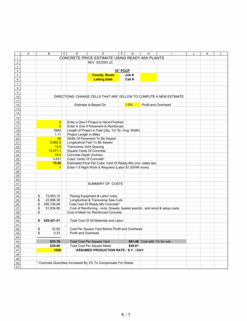
1234567891011121314

15161718192021222324252627282930313233343536373839404142434445464748495051

A B C D E F G H I J K L

REV. 02/2003 JC

10" PCCPCounty, Route Job #Letting Date Call #

DIRECTIONS: CHANGE CELLS THAT ARE YELLOW TO COMPUTE A NEW ESTIMATE

Estimate Is Based On 1.0% Profit and Overhead

0 Enter a One if Project is Hand-Finished0 Enter A One If Pavement Is Reinforced

5882 Length of Project in Feet ((Sq. Yd.*9) / Avg. Width)1.11 Project Length in Miles

20 Width Of Pavement To Be Sawed5,882.0 Longitudinal Feet To Be Sawed

15.0 Transverse Joint Spacing13,071.1 Square Yards Of Concrete

10.0 Concrete Depth (Inches)3,631 Cubic Yards Of Concrete*75.00 Estimated Price Per Cubic Yard Of Ready-Mix (incl. sales tax)

1 Enter 1 if Night Work is Required (Labor $1.50/HR more)

SUMMARY OF COSTS

73,953.15$ Paving Equipment & Labor costs22,896.38$ Longitudinal & Transverse Saw Cuts

280,736.68$ Total Cost Of Ready Mix Concrete*51,834.80$ Cost of Reinforcing - incls. Dowels, basket assmbl., and rerod & setup costs

-$ Cost of Mesh for Reinforced Concrete

429,421.01$ Total Cost Of All Materials and Labor

32.85$ Cost Per Square Yard Before Profit and Overhead0.33$ Profit and Overhead

----------------------$33.18 Total Cost Per Square Yard $41.48 Cost with 1% for sub$39.68 Total Cost Per Square Meter $49.61

1000 'ASSUMED PRODUCTION RATE - S.Y. / DAY

* Concrete Quantities Increased By 3% To Compensate For Waste

CONCRETE PRICE ESTIMATE USING READY-MIX PLANTS

123456789

1011121314151617181920212223242526272829303132333435363738394041424344454647484950515253545556

B C D E F G H I J KThe sawcut table below may be adjusted for labor and saws due to time restrictions.

The paving table below may be adjusted for labor and equipment. If the project is handwork, adjust the labor and zero the grade trimmer & pav. Train.

-------------------------------------------------------------------------- SAWCUT LABOR & EQUIP. COSTS (MEANS)

Wage * PER 8 HR. DAY Production rate2 1 equip. opr.(light) $37 584.00$ 2500 ft. per 8 hr. day1 1 teamster $27 212.00$ 13744.66667 total ft. of sawcut1 1 truck 15 120.00$ 14.0 days needed2 1 conc. Saw 14.58 233.28$ .1 1 water tank (65 gal.) 1.7 13.60$

---------------subtotal 1,162.88$

mob. 200.00$ * Note - Add $1.50 per hr. for all labor - Night Work o+p 20%

Total 1,635.46$

PAVING CREW & EQUIPMENT (MEANS)& AVG. LABOR IN MO.Crew & Equip. Wage * PER HR.

1 foreman $37.50 37.50$ 4 laborers $27.50 110.00$ 1 operators $36.50 36.50$ 1 rerodman $29.50 29.50$ 4 cement finisher $28.50 114.00$ 2 carpenters $29.50 59.00$ 1 skid loader 17.14$ 17.14$ 1 form screed 17.15$ 17.15$ 1 plate compactor 4.39$ 4.39$ 2 vibrator 0.55$ 1.10$

total/hr 426.28$

days needed 13

total cost/8 hr day 44,575.59$

PAVING CREW & EQUIPMENT (MEANS)& AVG. LABOR IN MO.Crew & Equip. Wage * PER HR.

1 foreman 37.50$ 37.50$ 6 laborers 27.50$ 165.00$ 3 operators 32.50$ 97.50$ 1 rerodman 29.50$ 29.50$ 6 cement finisher 28.50$ 171.00$ 1 grader 56.87$ 56.87$ 1 24' paver 100.46$ 100.46$ 1 cure/texture 23.20$ 23.20$ 1 backhoe 26.19$ 26.19$

total/hr 707.22$

days needed 13

total cost/8 hr day 73,953.15$

HAND FINISH

MACHINE FINISH

57585960616263646566676869707172737475767778798081828384858687888990919293949596979899100101102103104105106107108109110111112113114

B C D E F G H I J K

-----------------------------------------------------------------------

Set Up Costs

Assumptions:* Estimated String Line Production Time (4 Labor Man hours Per 500 Feet + 1 Foreman)

* Estimated Dowel Rod/Basket Producton Rate 1 Basket every 15 Ft (30' Width)With Dowell Rods Requires 2 Persons Per Basket Assbly. 15 Baskets Assembly's.Per Hour Equipment Cost @$50 Per Hour

Basket Assembly's.With Dowell Rods - Cost Per Foot $5.00

7,842.67 Number Of Basket Feet Required150.00 Basket Feet Per Hour52.28 Total Man Hours Required For Baskets

11,764.00 String Line Feet94.11 String Line Man Hours

39,213.33 Total Material Costs3,105.70 Labor Costs For String Line6,901.55 Labor Costs For Dowel Rod & Basket Assbly's.2,614.22 Equipment Costs

51,834.80Total Labor & Material Costs

-----------------------------------------------------------------------

-----------------------------------------------------------------Cost Of 5/8" Reinforcing Rods

For Longitudinal Joint

30" Centers30" LongOne Ton = 96 Pieces That Are 20' Long

23,040.00 Total Inches Per Ton768mber Of Units 30" Long Per Ton

$760.00 Cost Per Ton0.99 Cost Per 30" Piece

#REF! ber Of Pieces Required For Project#REF! Cost Of Re-Rods For The Project

-----------------------------------------------------------------

The following is the Estimators Spreadsheet on Hot Mix Asphaltic Concrete.This page is a summary sheet of inputs and the remaining pages are the actual spreadsheet.

Superpave Asphalt Spreadsheet Description

Items entered on a project by project basis on the front summary page.Rows 1-16Top of spreadsheet, rows 1-16, is used when asphalt is set up in area measure. Upper lifts thickness and edge length are obtained from the plans and used to calculate the quantity of wedge material to be included in the square yard price.The edge length is the total edge length so the estimator must calculate the linear feet of total edge length. This length isthen rounded up to the nearest 100 feet. Total quantities of the area items are totaled at the bottom of the tables, Row 18.

Rows 18-23 Column to the left, column H, are the items of Asphalt paid for by weight from the plans. The center column, column N, is a description including the letting month, county, route, asphalt mixes and asphalt performance grade. Indicate whichquarry that the bulk of the materials will come from or where the asphalt plant for the job will reside.

Description for the rest of the shaded cells. Profit and overhead, Cell N27, indicate the percentage for the profit and overhead for the project. MTV, cell H32, enter a 1 if an MTV is required for the project. The SMA cell, H28, is used if the sma fibers are not aseparate bid item.

Cell H36 requires the county number to be entered. The county number is used to look up the wage rates from the tablescontained in columns AP through BC. The wage rates are changed once a year when the new state wage rates are released. The highest of the State or Federal rate is used.

Cell H37 is for the number of miles from the refinery to the project midpoint. This mileage is used for projects that do not havea DBE requirement. For these jobs the mileage is used in the table located in columns U through Y to look up a cost for trucking based on mileage. The trucking costs are based on the old1993 PS&E rates but have been adjusted due to inflation/change in fuel costs since 1993. Conversations with trucking companies and back figuring quotes for hauling verify the rate chart.The mileage costs are used in a formula located in cell H43. Copy cell H43 up to cell H42 whenever there is no DBE requirement on the project. When there is a DBE requirement a hauling price per hunderweight obtained from a DBE hauling company is used for the asphalt hauling price. Enter DBE price per hunderweight into cell O42 from the DBE hauler's tables.

Cell H40 enter the asphalt price for the grade of asphalt in the mix. Price obtained from suppliers and Platt's oilgram.Actual price used is determined by discussion among the estimators about the % of the sources quotes to use.

O29 Through T39 Mix design table. Obtain closest mix design for your project from the archive of mixes. Enter mix %'sand location of sources. Obtain as many quotes as possible and delivered prices if possible. May need to adjust quotesafter discussion with other estimators. In row 38 enter in the mileage from the source to the project midpoint going through the asphalt plant location or the mileage from the asphalt plant to the project midpoint depending onwhether the quoted include any delivery. In row 39 enter in the aggregate price that will be used for the estimate factoringin 6% tax on the base material price. Use field office and district materials personnel for reference.

Cell Q59 enter a administration premium percentage for the price if asphalt is sub-contracted. Percentage varies due tothe total asphalt price compared to the price of the project.

Cell N62 enter production rate for project. Possible resource is the production rate chart in PDM Sect 4-03.16. Roundproduction so full days are used for project.

Equipment and Crew items are based on past MoDOT projects. Equipment rates are the monthly rates from the Blue Book divided by 175 hrs per month and have the hourly operating rate from the Blue Book applied. Equipment and crew are broken down into per hour costs and are factored into the per ton or area price based on the amount of time it will take to complete the work.

123456789

1011121314151617181920212223242526272829303132333435363738394041424344454647484950515253545556575859606162636465666768697071727374757677787980818283848586

A B C D E F G H K L M N O P Q R S TUpper Total Edgelifts mm Length M Thick mm AC -S.M. MA - S.M. Wedge CM TOT CM AC-FACT MA-FACT AC - MG MA - TONS

0 0 0 0 0 0.00 0.00 0.0000 0.0000 0.0 0.00 0 0 0 0 0.00 0.00 0.0000 0.0000 0.0 0.00 0 0 0 0 0.00 0.00 0.0000 0.0000 0.0 0.00 0 0 0 0 0.00 0.00 0.0000 0.0000 0.0 0.00 0 0 0 0 0.00 0.00 0.0000 0.0000 0.0 0.00 0 0 0 0 0.00 0.00 0.0000 0.0000 0.0 0.0

TOTALS 0.0 0.0Upper Total Edge

ASPHALT MIX PRICE ESTIMATE lifts IN Length ft Thickness AC -S.Y. MA - S.Y. Wedge CY TOT CY AC-FACT MA-FACT AC - TONS MA - TONSREV. 2-2003 0.00 0.00 0.00 0 0 0.00 0.00 0.0000 0.0000 0.0 0.0

0.00 0.00 0.00 0 0 0.00 0.00 0.0000 0.0000 0.0 0.00.00 0.00 0.00 0 0 0.00 0.00 0.0000 0.0000 0.0 0.00.00 0.00 0.00 0 0 0.00 0.00 0.0000 0.0000 0.0 0.00.00 0.00 0.00 0 0 0.00 0.00 0.0000 0.0000

Totals 0.0 0.0Feb. 2003 TOTALS 0.00 0.00

250.00 Tons of Asphalt (Resurf) St. Louis Co. Rte 15,000.00 Tons of Min. Aggr (Resurf) SP190LD MIX

PG 64-22 ASPHALT

ASSUME MATERIALS FROM: Someones Quarry

Estimate Is Based On A 1.0% Profit and Overhead250.0 Tons Of Asphalt Cement5,000 Tons Of Mineral Aggregate Gradation - (by weight)

Mix Ratio (Asphalt) 4.8% 10.0% 25.5% 36.0% 15.0% 12.0% 1.5% Mix Ratio (Aggregate) 95.2% 1" 3/4" 3/8" Man. Sand Porphory Hyd.

1 MTV Required? 1 - yes 0 - no Aggr Aggr Aggr Aggr Aggr Lime cost/lb. 0 SMA Mix? 1 - yes 0 - no

0.01 0 Pounds of Fibers (cellulose)5,250.00 Tons Of Mix 500.00 1,275.00 1,800.00 750.00 600.00 75.00

96 County: St. Louis10 Est Miles From The Refinery To Proj Midpt

24.48 Est Miles From The Plant To Proj Midpoint (avg) 12 12 12 12 110 6010.12 Aggr Price Per Ton At The Quarry (avg) 8.50 8.75 9.00 10.00 11.00 65.00

100.00 Asphalt Price Per Ton At The Refinery

121.60 Asphalt Price Including Transportation & Profit 0.58 DBE rate per cwt#VALUE!

MIX PRICE---------

4.82 Transportation Cost Per Ton Of Aggr (avg) 2.97 2.97 2.97 2.97 17.51 10.115.23 Equipment Cost Per Ton2.52 Labor Cost Per Ton4.70 Asphalt Cost Per Ton Of Mix Unit Extended

10.12 Aggregate Cost Per Ton Quanities Price Amount0.23 Profit and Overhead --------- -------- ------------ metric

250.0 121.60 30,400.00 134.0427.62 Mix Price per Ton 5,000.0 22.92 114,585.16 25.2630.44 Mix Price per Mg

5,250.0 144,985.1622.92 Aggregate Price Per Ton 0.05 metric

27.62 30.44 Mix Price121.60 Asphalt Price Per Ton

Aggregate Sub Price: 23.15 1 % Added for SubcontractingMetric Price: 25.51 27.83 Sub Mix Price(English)

3.79 Estimated Working Days 30.68 Sub Mix Price(Metric)1400 Production Rate - Tons/Day

Component Table

Thick Total Cost/SY Cost/SY Total "Subin. Cost AC MA Cost/SY MA

0.00 $0.00 #DIV/0! #DIV/0! #DIV/0! #DIV/0!0.00 $0.00 #DIV/0! #DIV/0! #DIV/0! #DIV/0!0.00 $0.00 #DIV/0! #DIV/0! #DIV/0! #DIV/0!0.00 $0.00 #DIV/0! #DIV/0! #DIV/0! #DIV/0!

Thick Total Cost/SM Cost/SM Totalmm Cost AC MA Cost/SM

0 $0.00 #DIV/0! #DIV/0! #DIV/0!0 $0.00 #DIV/0! #DIV/0! #DIV/0!0 $0.00 #DIV/0! #DIV/0! #DIV/0!0 $0.00 #DIV/0! #DIV/0! #DIV/0!0 $0.00 #DIV/0! #DIV/0! #DIV/0!0 $0.00 #DIV/0! #DIV/0! #DIV/0!

$0.00

123456789

1011121314151617181920212223242526272829303132333435363738394041424344454647484950515253545556575859606162636465666768697071727374757677787980818283848586

U V W X Y Z AA AB AC AD AE AF AG AH AI AJ AK AL AM AN AO

Equipment Costs(Source: Rental Rate Blue Book - 2003)

Updated: 2-2003Total % 8 Hr Day (assumed) 175 hrs per month100.0%

Rental RateOperating Total Prod. Prod.PSC Rates : Effective - 10/29/93 cost/hour cost/hour cost/hr Rate/ Rate/* Adjusted for fuel increase

Hour Day------------- ------------- -------- ----- -----

Min Curr Max Ave 68.57 20.00 88.57 Material Transfer Vehicle - CMI MTP-400A (assumed costs)Per Rate Per Per 8.23 12.85 21.08 Water Truck - 1500 gal

Miles Trip 15% Trip Trip 25.58 18.20 43.78 175 1,400 Wheel Loader - Cat 950F----- ---- ---- ---- ---- 37.20 22.40 59.60 Batch Plant - Cold Feed Bins (3 - 75 T CAP)

1 0.93 1.20 1.04 1.06 13.43 9.30 22.73 Batch Plant - Cold Feed Conveyors 30" x 34'2 1.06 1.36 1.18 1.20 133.01 93.75 226.76 Batch Plant - Port. Drum Mixer/Dryer - CMI-PVM 3003 1.19 1.53 1.33 1.35 50.63 32.40 83.03 Batch Plant - Wet Scrubber - 40,000 cfm4 1.32 1.70 1.48 1.50 37.28 22.30 59.58 Batch Plant - Self-Erecting Port. Surge Silo & Conveyors (300 T/hr)5 1.44 1.85 1.61 1.63 108.90 67.35 176.25 175 1,400 Asphalt Paver - Barber Greene BG-265B6 1.57 2.02 1.76 1.78 6.96 2.95 9.91 Grade Control, Paver - Electric7 1.70 2.19 1.90 1.93 23.10 9.15 32.25 Rubber Tired Roller - Bomag BW11R8 1.82 2.35 2.04 2.07 39.96 19.15 59.11 Tandem Vibratory Drum Roller - Bomag BW202ADSH (84")9 1.95 2.51 2.18 2.21 14.14 9.40 23.54 Static Steel Drum Roller - Tandem 10 Ton - Ingersoll-Rand ST75

10 2.07 2.67 2.32 2.35 173 1,386 Adjusted Production Rate Due To 1% Waste11 2.19 2.82 2.45 2.49 5.23 Total Equipment Cost Per ton12 2.30 2.97 2.58 2.6213 2.41 3.11 2.70 2.7414 2.51 3.23 2.81 2.85 Labor Costs15 2.63 3.39 2.95 2.9916 2.72 3.51 3.05 3.09 Updated: 200217 2.82 3.63 3.16 3.20 Hourly18 2.91 3.75 3.26 3.31 Rate No. Req'd19 3.01 3.88 3.37 3.42 ------20 3.08 3.97 3.45 3.50 32.76 12 Paver Operator 121 3.16 4.07 3.54 3.59 32.76 12 Roller Operators 322 3.23 4.16 3.62 3.67 32.76 12 Asphalt Plant Operator 223 3.32 4.28 3.72 3.77 29.38 12 Asphalt Plant Laborers 124 3.39 4.37 3.80 3.85 29.38 12 Laborers (Includes 2 for Traffic C 625 3.47 4.52 3.93 3.97 35.00 Foreman 126 3.55 4.68 4.07 4.1027 3.64 4.84 4.21 4.23 2.52 Total Labor Cost Per Ton28 3.75 5.00 4.35 4.3729 3.86 5.16 4.49 4.5030 3.97 5.32 4.63 4.6431 4.08 5.49 4.77 4.78

32 4.19 5.65 4.91 4.92

87888990919293949596979899100101102103104105106107108109110111112113114115116117118119120121122123124125126127128129130131132133134135136137138139140141142143144145146147148149150151152153154155156157158159160161162163164165166167168169170171172173

U V W X Y Z AA AB AC AD AE AF AG AH AI AJ AK AL AM AN AO33 4.30 5.80 5.04 5.0534 4.41 5.96 5.18 5.1835 4.52 6.12 5.32 5.3236 4.63 6.28 5.46 5.4637 4.75 6.44 5.60 5.6038 4.85 6.60 5.74 5.7339 4.97 6.76 5.88 5.8740 5.07 6.92 6.02 6.0041 5.19 7.08 6.16 6.1442 5.30 7.25 6.30 6.2843 5.41 7.41 6.44 6.4244 5.52 7.57 6.58 6.5645 5.63 7.72 6.71 6.6946 5.74 7.88 6.85 6.8247 5.85 8.04 6.99 6.9648 5.96 8.20 7.13 7.1049 6.07 8.36 7.27 7.2350 6.18 8.52 7.41 7.3751 6.29 8.68 7.55 7.5152 6.40 8.84 7.69 7.6453 6.51 8.99 7.82 7.7754 6.62 9.15 7.96 7.9155 6.73 9.32 8.10 8.0556 6.84 9.48 8.24 8.1957 6.95 9.64 8.38 8.3258 7.06 9.80 8.52 8.4659 7.17 9.96 8.66 8.6060 7.28 10.11 8.79 8.7361 7.38 10.27 8.93 8.8662 7.50 10.43 9.07 9.0063 7.61 10.59 9.21 9.1464 7.71 10.75 9.35 9.2765 7.83 10.90 9.48 9.4066 7.95 11.06 9.62 9.5467 8.05 11.22 9.76 9.6868 8.17 11.39 9.90 9.8269 8.28 11.55 10.04 9.9670 8.39 11.70 10.17 10.0971 8.50 11.86 10.31 10.2272 8.61 12.02 10.45 10.3673 8.72 12.18 10.59 10.5074 8.83 12.33 10.72 10.6375 8.94 12.49 10.86 10.7676 9.05 12.65 11.00 10.9077 9.17 12.81 11.14 11.0478 9.28 12.96 11.27 11.1779 9.39 13.12 11.41 11.3180 9.50 13.28 11.55 11.4481 9.61 13.44 11.69 11.5882 9.72 13.60 11.83 11.7283 9.83 13.75 11.96 11.8584 9.94 13.92 12.10 11.9985 10.05 14.08 12.24 12.1286 10.16 14.23 12.37 12.2587 10.27 14.39 12.51 12.3988 10.38 14.55 12.65 12.5389 10.49 14.70 12.78 12.6690 10.60 14.86 12.92 12.7991 10.71 15.02 13.06 12.9392 10.83 15.18 13.20 13.0793 10.93 15.33 13.33 13.2094 11.04 15.49 13.47 13.3395 11.15 15.65 13.61 13.4796 11.26 15.80 13.74 13.6097 11.38 15.96 13.88 13.7498 11.49 16.12 14.02 13.8899 11.60 16.27 14.15 14.01

100 11.71 16.43 14.29 14.14

123456789

1011121314151617181920212223242526272829303132333435363738394041424344454647484950515253545556575859606162636465666768697071727374757677787980818283848586

AP AQ AR AS AT AU AV AW AX AY AZ BA BB BC BD

Labor Rates - Rev. 10-2002

Skilled OperatingOperating Laborer Labor Operating Engineer

County Laborer Engineer Zone Laborer Hourly Engineer HourlyNumber Zones Zones County Name District Conversion Zone Rate* Zone Rate*

------ ------- --------- ------------ -------- ---------- --------- ------ -------- --------1 3 2 Adair 2 E1 = 1 1 $28.65 1 37.162 22 4 Andrew 1 E2 = 2 2 $28.86 2 33.583 22 4 Atchinson 1 E3 = 3 3 $27.20 3 31.154 3 2 Audrain 3 E3E = 33 4 $27.20 4 27.225 22 5 Barry 7 E4 = 4 5 $27.45 5 37.166 22 5 Barton 7 E5 = 5 11 $28.70 67 22 4 Bates 7 KC = 11 12 $29.38 11 32.768 22 4 Benton 5 STL = 12 21 $30.21 12 37.169 3 2 Bollinger 10 W1 = 21 22 $25.63

10 3 2 Boone 5 W2 = 22 33 24.1811 21 3 Buchanan 112 3 2 Butler 10 *Includes Fringe Benefits13 22 4 Caldwell 114 3 2 Callaway 515 22 5 Camden 516 3 2 Cape Gir. 1017 22 4 Carroll 218 3 2 Carter 919 21 3 Cass 420 22 5 Cedar 721 3 4 Chariton 222 22 5 Christian 823 3 2 Clark 324 11 11 Clay 1125 22 3 Clinton 126 3 2 Cole 527 3 4 Cooper 528 3 2 Crawford 9

29 22 5 Dade 7

87888990919293949596979899100101102103104105106107108109110111112113114115116117118119120121122123124125126127128129130131132133134135136137138139140141142143144145146147148149150151152153154155156157158159160161162163164165166167168169170171172173

AP AQ AR AS AT AU AV AW AX AY AZ BA BB BC BD30 22 5 Dallas 831 22 4 Daviess 132 22 4 DeKalb 133 3 2 Dent 934 22 5 Douglas 835 3 2 Dunklin 1036 1 1 Franklin 637 3 2 Gasconade 538 22 4 Gentry 139 22 5 Greene 840 22 4 Grundy 241 22 4 Harrison 142 22 4 Henry 443 22 5 Hickory 844 22 4 Holt 145 3 4 Howard 246 3 2 Howell 947 3 2 Iron 948 11 11 Jackson 1149 22 5 Jasper 750 5 1 Jefferson 651 22 4 Johnson 452 3 2 Knox 353 22 5 Laclede 854 21 3 Lafayette 455 22 5 Lawrence 756 3 2 Lewis 357 4 1 Lincoln 358 3 4 Linn 259 22 4 Livingstn 260 22 5 McDonald 761 3 2 Macon 262 3 2 Madison 1063 3 2 Maries 564 3 2 Marion 365 22 4 Mercer 266 3 2 Miller 567 3 2 Miss. 1068 3 2 Moniteau 569 3 2 Monroe 370 4 2 Montgomey 371 22 2 Morgan 572 3 2 New Madrd 1073 22 5 Newton 774 22 4 Nodaway 175 3 2 Oregon 976 3 2 Osage 577 22 5 Ozark 878 3 2 Pemiscot 1079 3 2 Perry 1080 22 4 Pettis 581 3 2 Phelps 982 3 2 Pike 383 11 11 Platte 484 22 5 Polk 885 3 2 Pulaski 986 3 2 Putnam 287 3 2 Ralls 388 3 2 Randolph 289 11 11 Ray 490 3 2 Reynolds 991 3 2 Ripley 992 2 1 St. Charl 693 22 5 St. Clair 794 3 2 St. Franc 1095 3 2 Ste. Gene 1096 12 12 St. Louis 1297 22 4 Saline 298 3 2 Schuyler 299 3 2 Scotland 3

100 3 2 Scott 10101 3 2 Shannon 9102 3 2 Shelby 3103 3 2 Stoddard 10104 22 5 Stone 8105 3 4 Sullivan 2106 22 5 Taney 8107 3 2 Texas 9108 22 5 Vernon 7109 4 1 Warren 3110 3 2 Washingto 9111 3 2 Wayne 10112 22 5 Webster 8113 22 4 Worth 1114 22 5 Wright 8115 12 12 St Lou Cy 12

__________________________________________________

APPENDIX L

Alternate Bid on Pavements

Process and Job Special Provision

L-2

Alternate Bid Process

The following are guidelines from MoDOT’s Project Development Manual explaining to designers how to prepare plans with alternate bids on pavements: 6-03.3 ALTERNATE PAVEMENTS. To ensure that every effort is being made to increase the

competition for paving contracts, and that the latest market rate is considered when determining pavement type, contractors will be allowed to bid a selected alternate design. This will enable contractors to structure their bid around availability of suppliers, materials and use methods they are confident in performing. By utilizing alternate bids the result of equivalent long term pavement rehabilitation at the best value for our highway dollars will be obtained. Future maintenance costs will be considered with a life cycle cost adjustment factor, thus resulting in the most equivalent specifications possible to draw in the maximum number of bidders for MoDOT paving projects. Formulation of the alternate pavement methods were completed by a pavement team consisting of MoDOT as well as representatives from the asphalt and concrete industries.

6-03.3 (1) ALTERNATE OPTIONS. Alternate pavement scenarios include for full depth: full

depth concrete vs. full depth superpave or bituminous pavement for designs with an equivalent asphalt thickness 8 inches [200 mm] or greater; for long-term pavement rehabilitation: unbonded concrete overlay vs. superpave asphalt over rubbilized pavement. These options will be bid as alternate options with the inclusion of a life cycle cost adjustment factor which will be added to the lowest asphalt bid to take into consideration the future rehabilitation cost for each pavement type. This life cycle cost adjustment factor considers future cold milling and overlay of the surface layer of asphalt at 20 and 33 year intervals and diamond grinding of the concrete surface at 20 years. The last published real interest rates from the United States Office of Management and Budget will be used to bring the future costs to present worth. GHQ Design will calculate the cost adjustment factor utilizing the most updated information available.

6-03.3 (2) ADDITIONAL SELECTION CRITERIA. All major paving projects should be

designed with alternate bids for pavements in mind. Generally this will include projects over two lane-miles in length with an equivalent asphalt thickness of 8 inches or greater, but projects should be evaluated on a case-by-case basis. A lane is defined as pavement 12 ± 2 feet (3.6 ± 0.6 m) wide. Full depth paved shoulder widths that have the same pavement type as the mainline should be included in calculating lane miles.

Pavements that meet the above criteria, but have constructability or other prevailing

issues that makes only one type of pavement construction desirable should be justified why alternate bids on pavement for that project is not feasible. This may include circumstances such as widening existing pavements, urban construction, consideration of how the pavement type effects the major item of work for the project (example if major item of work for the project is bridge work the life cycle costs may be insignificant to the total project cost), total amount of paving compared to existing pavement, project staging and project scoping with regard to long-range transportation goals. The documentation should be submitted to GHQ Design for

L-3

approval with assistance from GHQ Construction and Materials. All interstate projects, with the exception of 4R projects on Route I-70 or 4R projects

involving short-term rehabilitation strategies, will normally involve alternate bids on pavements. The rehabilitation strategy for interstate routes should be alternate bids on pavements with the alternates being an 8" concrete unbonded overlay over a 1" AC bond breaker or 1 3/4" SP125HBSM over 3" SP250HB over 7 1/4" SP250HC over rubblized concrete pavement. The two upper lifts of the HMA overlay need to use polymer modified asphalt in accordance with Section 6-07 and the remaining lifts PG 64-22 asphalt binder. Justification must be given and approval received from GHQ to use anything less than these two alternates, such as a 7 3/4" AC overlay. Route I-70 has been exempted from alternate bids at this time because long-term rehabilitation strategies are not under consideration until it has been established what existing lanes will be used in the future capacity expansion of the facility.

6-03.3 (3) ALTERNATE ESTIMATES. For projects that are defined as candidates for

alternate bids on pavements, it is recommended that job cost estimations during the early scoping stages of the project be based upon the following:

(a) For projects involving new construction, base costs on the construction of

concrete pavement, using the appropriate design thickness provided in Figure 6-03.12.

(b) For projects involving a concrete unbonded overlay, base costs on the construction of a 9-inch (225 mm) concrete unbonded overlay as the design thickness. The additional one inch thickness is to allow for adjustment of the profile grade in order to eliminate existing undulations in the pavement and to re-establish a smooth profile grade. See Subsection 6-05.18 for guidance on reestablishing a smooth profile grade on concrete unbonded overlay projects.

The following are design guidelines for different project scenarios: 6-03.3 (4) GRADING PROJECT SEPARATE FROM PAVING WITH HEAVY DUTY

PAVEMENT AND 18 IN. [0.45 m] ROCK BASE. (For medium and light duty pavements with 18 in. [0.45 m] rock fill base there is no difference in pavement thickness between concrete and asphalt pavement designs.)

• For this scenario, there will only be a 1” maximum difference in pavement

thickness between concrete and asphalt pavement designs. • The subgrade profile should be designed for the concrete pavement alternate. • If asphalt pavement is constructed, there should be no adjustment to the

subgrade. Rather, the asphalt pavement should be built on grade resulting in a 1” increase in the profile grade. At critical conflict points such as bridge ends or grade separations, the subgrade should be transitioned to provide the correct clearance or to match profile grade at a rate of 1200:1.

• Profile grade transitions at bridges and grade separations are paid for as sub-grading and shouldering, class 1. The pay item subgrading and shouldering, class 1, typically is a job length quantity, which in this case would include the mentioned transitions.

L-4

6-03.3 (5) GRADING PROJECT SEPARATE FROM PAVING PROJECT, WITHOUT 18

IN. [0.45 m] ROCK BASE. (Maximum difference between concrete and asphalt pavement design is 8 inches [200 mm].)

• Grading project is designed for concrete pavement design. • The design profile grade is maintained for either alternate pavement. • In the paving project the removal of sub-grade material for asphalt pavement

design will be paid for as subgrading and shouldering, class 1. • Design profile to accommodate minimum cover (asphalt pavement thickness

should control) of crossroad structures. 6-03.3 (6) GRADING AND PAVING TOGETHER IN ONE PROJECT.

• Design for pavement as per pavement type selection process outlined in Section 6-03.2 (Alt. A).

• Design profile grade to accommodate minimum cover (asphalt pavement thickness should control) of crossroad structures.

• Cross sections designed for pavement as per pavement type selection process (Alt. A), with added or deducted yardages for Alternate B noted in profile balances of the plan/profile sheets.

6-03.3 (7) PLANS FOR ALL ALTERNATE BIDS FOR PAVEMENT PROJECT. Plans for all alternate bids for pavement projects should contain:

• Typical sections for both alternates, including station limits, and all side road

connections shall have the pavement type designated. • One set of 2B sheets with Alt. A and Alt. B items separated by alternate and

clearly labeled. • Using the “Estimate 2000” program, the pavement, base and grading

quantities for Alternate A should be designated as “Section 02” and the pavement, base and grading quantities for Alternate B should be designated “Section 03”. This will enable summation of the appropriate subtotals to compile an estimate total cost per alternate.

• Certain pay items should not be repeated in “Section 01” and an alternate section, “Section 02 or 03”. For example Class A should not show up twice in the same project, this would lead to differing bids for Class A and cause confusion when administering the contract. If the Class A quantities differ include the appropriate total Class A quantity in each of the alternates.

• Design Special Provision-ALTERNATE FOR PAVEMENTS DSP-96-04F. Life Cycle Cost adjustment factor to be calculated by Headquarters office.

• All pay items for pavements shall be in tons • To calculate the Life Cycle Cost Analysis factor, quantities for the traveled

way are needed. These quantities need to be included with the submittal letter. For example the traveled way will include 12 ft lanes [3.6 m] for

L-5

mainline and 18 ft [5.4 m] lanes for ramps, any area considered as shoulder is not the traveled way.

L-6

The following is the job special provision that will be inserted in contracts allowing alternate bids on pavements: ALTERNATES FOR PAVEMENTS DSP-96-04F 1.0 Description. This work shall consist of a pavement composed of either Portland cement concrete or asphaltic concrete, constructed on a prepared subgrade in accordance with the standard specifications and in conformity with the lines, grades, thickness and typical cross sections shown on the plans or established by the engineer. 2.0 Alternates. To exercise this option, separate pay items, descriptions and quantities are included in the itemized proposal for each of the two alternates. The bidder shall bid only one of the two alternates and either enter “0” or leave blank in the contract unit price column for any pay item listed for the other alternate. 2.1 A sum of $_______ (amount to be inserted by GHQ) will be added by the Commission to the total bid using the asphalt alternate for bid comparison purposes to factor in life cycle cost analysis of the roadway. The additional amount added will not represent any additional payment to be made to the successful bidder and is used only for determining the low bid. 2.2 The quantities shown for each alternate reflect the total square yards [meters] of pavement surface designated for alternate pavement types as computed and shown on the plans. No additional payment will be made for asphaltic concrete mix quantities to construct the required 1:1 slope along the edge of the pavement. 2.3 The profile grade shown on the plans was designed for (concrete/asphaltic concrete) pavement. Adjustment for (asphaltic concrete/concrete) will require additional grading or embankment. Any additional grading or embankment required to bring the roadway subgrade to the proper elevation for either alternate shall be paid for completely under the pay items included in the contract. (Optional for previously graded roadbeds that require only subgrading and shoulder and compacting embankment “In the case of a previously graded roadbed any excavation necessary to prepare the subgrade for either alternate shall be completely covered in the Subgrading and Shouldering pay item”) 3.0 Method of Measurement. The quantities of concrete pavement will be paid for in accordance with Section 502.14 of the Pavement Specification for alternate bids job special provision included in the contract. The quantities of asphaltic concrete pavement will be paid for in accordance with payment for bituminous material by the square yard (meter) job special provision included in the contract. 4.0 Basis of Payment. The accepted quantity of the chosen alternate and other associated items will be paid for at the unit price for each of the appropriate pay items included in the contract.

APPENDIX M

Interim HMA Overlay on Rubblized PCC Design Method

M-2

Design Method The empirical AASHTO design method for flexible pavements, currently used by MoDOT for other HMA designs, was used to estimate the HMA overlay thickness required for a typical rubblized 8” JRCP on 4” of Type 3 base material. Design Inputs Most design inputs were AASHTO-recommended values for the high volume arterials that might receive this rehabilitation treatment as shown below.

AASHTO Pavement Design Input Assumptions Initial Serviceability Level = 4.5

Terminal Serviceability Level = 3.0 Reliability = 90%

Overall Standard Deviation = 0.44 Total ESALs = 100,000,000

Rubblized PCC Thickness = 8" Rubblized PCC Drainage Coefficient = 1.0

Type 3 Base Thickness = 4” Type 3 Base Structural Coefficient = 0.07

Type 3 Drainage Coefficient = 0.90 HMA Overlay Structural Coefficient = 0.44

The Team needed additional guidance for two inputs, subgrade resilient modulus (MR) and rubblized PCC layer coefficient. The MoDOT Geotechnical Unit was asked to provide the subgrade MR expected under existing Interstate pavements. They estimated that the subgrade, in a saturated state, may have an MR as low as 1,000 to 2,500 (psi), and in a semi-saturated condition, range between 7,000 to 10,000 (psi). For the rubblized PCC layer coefficient data was gathered from other sources. A nationwide survey by the Florida DOT of other States rubblization treatments yielded a coefficient range from 0.10 to 0.30. The National Asphalt Pavement Association publication, ‘Guidelines for Use of HMA Overlays to Rehabilitate PCC Pavements’ (IS-117), recommends a range from 0.20 (for 99 percent reliability) to 0.35 (for 75 percent reliability). The 1993 AASHTO Guide recommends values from 0.14 to 0.30. Design Thicknesses Using the information above, HMA overlay pavement thicknesses on rubblized PCC were gernerated with the AASHTO design-based DARWin software program. A thickness sensitivity run was performed using three levels of subgrade MR and rubblized layer coefficients. The results are shown below.

M-3

DARWin 3.1 Analysis of HMA Overlay on Rubblized PCC

Subgrade MR

(psi) Rubblized PCC

Layer Coefficient HMA Overlay Thickness

(inches) 2000 0.22 18.5 2000 0.26 17.8 2000 0.30 17.1 5000 0.22 13.3 5000 0.26 12.6 5000 0.30 11.8 8000 0.22 11.0 8000 0.26 10.3 8000 0.30 9.6

The results represented worst case and best case scenarios. HMA overlays on rubblized pavements with subgrade MR ≤ 2000 (psi) or less are unlikely, because of problems with operating construction equipment rutting the PCC surface. It’s also unlikely that many pavements would have semi-saturated conditions during the major part of the year, particularly with the lack of drainage that exists under most corridors, therefore the higher modulus results could not be depended on. An average MR ~ 5000 (psi) seemed the most realistic foundation support for the rubblized PCC and the resulting thicknesses were judged reasonable for the heavy traffic that is expected on these roads. Therefore, a 12” of HMA was selected as the interim design overlay thickness on rubblized PCC.