patterns of international business cycles - october 2020

Patterns of international business cycles

Early in 2020, a long upswing in the global economy came to an abrupt end. The novel corona-

virus spreading around the world and the measures taken to contain it were accompanied by a

dramatic slump in activity and culminated in a crisis of historic proportions. The root causes of

earlier economic downturns were often less obvious. Analysing suitable indicators in order to

identify signs of a cyclical downturn at an early stage is, however, a key task for a forward-

looking monetary policy. Recessions are, for example, often preceded by signs of overheating

that are likely to be associated with a heightened vulnerability to crises. Relevant warning signals

can provide valuable insights for predicting cyclical turning points.

Indeed, empirical studies suggest that cyclical turning points – at least when seen with the bene-

fit of hindsight – often announced themselves in advance. For example, the longer an upswing

lasted, the greater was the probability that it would soon end. In most cases, a period of higher-

than- average aggregate rates of expansion was followed by a soft patch in which GDP growth

fell below its trend, and only rarely by a severe recession. Recessions in advanced economies

were often indicated by a flattening of the yield curve, or followed sharply accelerating oil prices.

The inclusion of such variables improves the accuracy of models for recession forecasting. Even

so, the models would not have identified some crises in advance and have forecast recessions

that failed to materialise.

Quantitative models can therefore send important warning signals before cyclical turning points.

Economic observers will still be taken by surprise by downturns in the future, however. But this

should not be viewed as a failure of empirical business cycle research. Even economies that pre-

viously appeared to be fairly resilient can be plunged into recession by shocks of sufficient mag-

nitude. This year’s global economic crisis is one example of this.

Deutsche Bundesbank Monthly Report

October 2020 41

Introduction

At the beginning of 2020, the coronavirus pan-

demic brought an extended upswing in the

global economy to a sudden end. The spread

of the virus and the measures taken to contain

the number of infections led within a matter of

weeks to a dramatic slump in activity, finally

culminating in an economic crisis of historic

proportions. Although the easing of the restric-

tions saw activity picking up rapidly, the recov-

ery has remained incomplete so far given the

ongoing risks of infection and constraints that

remain in place.

Even in the past, growth paths did not run

along straight lines. Rather, they were repeat-

edly interrupted by soft patches – in other

words, minor setbacks or periods of below

average rates of expansion. Dramatic declines

in macroeconomic activity – recessions – are

also on record for almost every economy.

Periods of high macroeconomic underutilisa-

tion are typically accompanied by deflationary

pressure on consumer prices. This may call for

timely monetary policy intervention, especially

given its time- lagged effects. Against this back-

drop, the analysis and forecasting of macro-

economic fluctuations – also known as the

business cycle – have always been a key focus

of applied macroeconomics.

For economic forecasting and the formulation

of recommendations for monetary policy, an

understanding of macroeconomic processes

and their key drivers is essential. Modern busi-

ness cycle models represent recessions mainly

as the outcome of unexpected events known

as shocks.1 These include, say, unanticipated

policy measures, technological advances, nat-

ural disasters, changes in preferences as well as

modified expectations and risk assessments.

Other possible triggers include unexpected

international developments that can be trans-

mitted through various channels, such as inter-

national trade and cross- border financial rela-

tionships. This means that cyclical swings are

very difficult to predict. Price rigidities, financial

market imperfections and other frictions can

delay the effects of shocks, prolong them and

also amplify them. It is, above all, the delays

that give economic observers the opportunity

to identify nascent downturns at an early stage.

Moreover, during a period of expansion there is

often an increase in vulnerabilities owing, for

example, to exaggerations in the financial sys-

tem. This means that, in mature upswings,

comparatively small shocks could trigger major

turmoil.2 Timely identification of vulnerabilities

would then make it possible to predict cyclical

turning points or, at least, estimate their prob-

ability.

Identification of cyclical turning points

Quantitative analysis of macroeconomic down-

turns and estimating the probability of their oc-

currence require not only an understanding of

macroeconomic processes but also an empir-

ical definition. In the traditional classification of

business cycle phases, a recession describes a

period of declining economic activity. This def-

inition is used as the basis for business cycle

dating, for example, by the National Bureau of

Economic Research (NBER) for the United

States and the Centre for Economic Policy Re-

search (CEPR) for the euro area, both of which

are widely recognised as official. A recession

follows a peak in aggregate output and, after a

trough, moves into an expansion. In order to

be classified as a recession, the contraction also

has to last at least a few months, be broad-

based and must not be confined to a small

Pandemic brings an end to multi- year global upswing

Recessions call for swift monet-ary policy inter-vention

Shocks the cause of cyclical fluctuations

Significance of fragilities

Recessions often defined by way of declining eco-nomic activity

1 Slutzky (1937) and Frisch (1933) laid the groundwork for the interpretation of economic processes as a sequence of shocks, which was then incorporated into modern eco-nomic models by Brock and Mirman (1972), Lucas (1972), as well as Kydland and Prescott (1982). The Bundesbank’s Dynamic Stochastic General Equilibrium (DSGE) model is one instance of a more comprehensive model of this class. For a more detailed description, see Hoffmann et al. (2020).2 For recent approaches that capture this in macroeco-nomic models, see Gorton and Ordoñez (2014), Boissay et al. (2016) as well as Paul (2020).

Deutsche Bundesbank Monthly Report October 2020 42

Measuring classical business cycles

Classical business cycles are characterised

by alternating periods of increasing and

declining economic activity. To date these

cycles, the literature often applies a rule-

based procedure developed by Bry and

Boschan (1971) to an indicator of macro-

economic activity.1 Expert- based methods

are an alternative approach in which special

committees identify the phases of the busi-

ness cycle on the basis of several statistical

procedures and a subjective assessment of

a number of macroeconomic indicators. In

the United States, for example, the Business

Cycle Dating Committee at the National

Bureau of Economic Research (NBER),

founded in 1978, employs a generally ac-

cepted classifi cation of economic activity

into expansionary and recessionary phases.2

The Business Cycle Dating Committee at the

Centre for Economic Policy Research (CEPR)

has been determining economic peaks and

troughs for the euro area since 2003.3 A

comparable classifi cation of business cycle

phases in Germany was presented by the

German Council of Economic Experts (SVR)

in 2017.4

Given the conceptual disparities, the ques-

tion arises as to how the dates determined

using mechanical methods differ from ex-

pert assessments. In order to make a com-

parison possible, the cyclical turning points

for the economic areas mentioned above

are calculated using the Bry- Boschan algo-

rithm. The respective seasonally adjusted

quarterly values of real gross domestic

product (GDP) for the period from the fi rst

quarter of 1970 to the second quarter of

2020 are used as an indicator of economic

activity.5

On balance, the dating of the cycles ac-

cording to the Bry- Boschan algorithm is

broadly in line with the experts’ assess-

ment.6 This is particularly true of the United

States and the euro area. Differences exist

only in the identifi cation of individual turn-

ing points and the classifi cation of phases

with low and, in some cases, negative GDP

growth rates. For example, the recession in

the United States identifi ed by NBER experts

in 2001 is not recognised. Furthermore, the

algorithm shows a brief downturn for the

euro area in the early 1980s, while the CEPR

Committee registers a prolonged contrac-

tion.7 A similar picture emerges for Ger-

many in the fi rst half of the 1980s, although

the Bry- Boschan algorithm identifi es two

short periods of contraction during the

longer- lasting recession identifi ed by the

SVR. There are further deviations for Ger-

many in the fi rst half of the 2000s and

around the end of 2012 and the beginning

of 2013.

The Bry- Boschan algorithm, in line with the

NBER experts’ assessment, dates the start

of the economic downturn in the United

1 The procedure recognises peaks and troughs in a time series if their level was lower or higher in the period before and after. Further conditions ensure a minimum cycle length and guarantee that each peak is preceded by a trough.2 See National Bureau of Economic Research (2020b).3 See Centre for Economic Policy Research (2020).4 See German Council of Economic Experts (2017).5 The data on macroeconomic activity for the euro area aggregate for the period prior to the establish-ment of the monetary union are taken from the Euro Area Business Cycle Network’s Area Wide Model (AWM) database. GDP data for Germany are data for West Germany up to and including the year 1991.6 The version of the Bry- Boschan algorithm adapted by Harding and Pagan (2002) for use in quarterly time series is used to date the turning points. It is customar-ily assumed that a business cycle comprises at least fi ve quarters and that a cyclical expansion or recession each last at least two quarters.7 Developments in investment and employment, which, in contrast to real GDP, recorded a signifi cant and steady decline in the period in question, were a key factor in the CEPR experts’ decision; see Centre for Economic Policy Research (2003).


October 2020 43

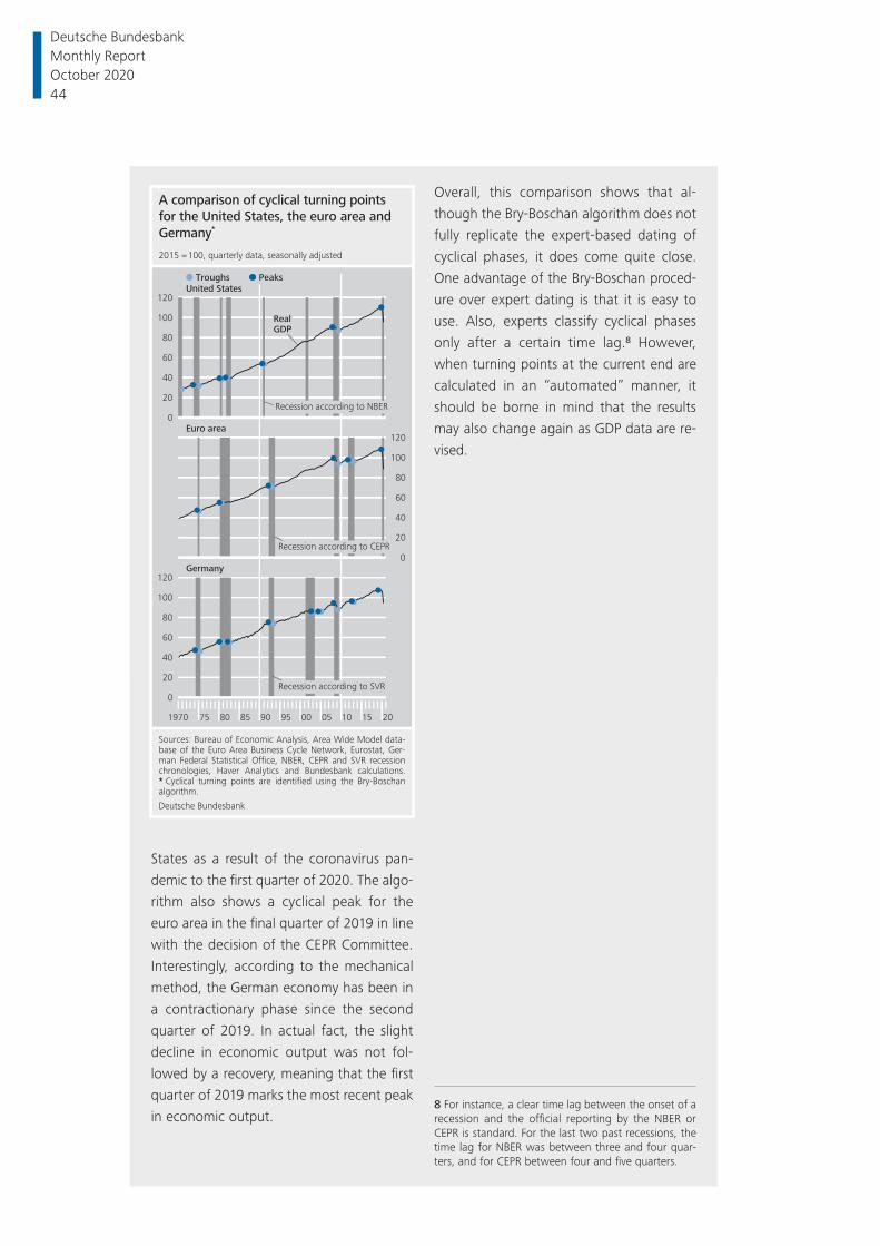
States as a result of the coronavirus pan-

demic to the fi rst quarter of 2020. The algo-

rithm also shows a cyclical peak for the

euro area in the fi nal quarter of 2019 in line

with the decision of the CEPR Committee.

Interestingly, according to the mechanical

method, the German economy has been in

a contractionary phase since the second

quarter of 2019. In actual fact, the slight

decline in economic output was not fol-

lowed by a recovery, meaning that the fi rst

quarter of 2019 marks the most recent peak

in economic output.

Overall, this comparison shows that al-

though the Bry- Boschan algorithm does not

fully replicate the expert- based dating of

cyclical phases, it does come quite close.

One advantage of the Bry- Boschan proced-

ure over expert dating is that it is easy to

use. Also, experts classify cyclical phases

only after a certain time lag.8 However,

when turning points at the current end are

calculated in an “automated” manner, it

should be borne in mind that the results

may also change again as GDP data are re-

vised.

8 For instance, a clear time lag between the onset of a recession and the offi cial reporting by the NBER or CEPR is standard. For the last two past recessions, the time lag for NBER was between three and four quar-ters, and for CEPR between four and fi ve quarters.

A comparison of cyclical turning points

for the United States, the euro area and

Germany*

Sources: Bureau of Economic Analysis, Area Wide Model data-

base of the Euro Area Business Cycle Network, Eurostat, Ger-

man Federal Statistical Office, NBER, CEPR and SVR recession

chronologies, Haver Analytics and Bundesbank calculations.

* Cyclical turning points are identified using the Bry-Boschan

algorithm.

Deutsche Bundesbank

1970 75 80 85 90 95 00 05 10 15 20

0

20

40

60

80

100

120

2015 = 100, quarterly data, seasonally adjusted

0

20

40

60

80

100

120

United States

Recession according to NBER

Germany

Euro area

Recession according to CEPR

RealGDP

0

20

40

60

80

100

120

Recession according to SVR

PeaksTroughs


number of sectors or regions of the economy.3

As a preferred measure for aggregate eco-

nomic activity, both the NBER and the CEPR

therefore use gross domestic product (GDP) ad-

justed for seasonal effects and price move-

ments. However, other quarterly time series are

additionally taken into consideration – such as

gross national income in the United States or

the production and expenditure- side GDP com-

ponents as well as employment in the euro

area. As the NBER aims at a monthly chron-

ology of the business cycles, selected higher-

frequency indicators are also analysed.4 On

both sides of the Atlantic, this is the basis on

which a committee of experts defines cyclical

peaks and troughs – otherwise known as cyc-

lical turning points.5

In cyclical analysis as well as academic research,

expert- based dating as well as heuristic tech-

niques and quantitative methods are used for

defining turning points. The latter have the ad-

vantage that they can be applied in accordance

with uniform criteria to a large group of coun-

tries. In some cases, cyclical movements can be

classified more rapidly on this basis. This is es-

pecially true when it comes to the widespread

concept of a “technical” recession, which is de-

fined as two or more consecutive quarters of

negative (seasonally adjusted) GDP growth.6

Often, the Bry- Boschan algorithm is applied as

an alternative.7 This approach identifies peaks

in a time series if the level was previously and

subsequently lower. When analysing quarterly

GDP time series, the two preceding and subse-

quent quarters are typically taken into consid-

eration. Furthermore, the specification of the

algorithm ensures a minimum cycle length and

the sequence of peaks and troughs.8 Even

though the procedure is quite simple, the re-

cession dates obtained in this way for major

economies largely correspond to the judge-

ment of experts (see the box on pp. 43 f.).

Even when there is no major crisis, the macro-

economic growth process seldom takes a

steady course. Instead, there are typically alter-

nating periods of rapid and slow growth. If

phases of slow economic expansion – known

as soft patches – persist for an extended period,

the associated welfare losses can in fact be

greater than those experienced in brief reces-

sions. With this in mind, greater attention has

been paid over the past few years to analysing

cyclical patterns of trend- adjusted time series,

especially of real GDP.9 As defined in this way, a

downturn would set in as soon as economic

output – following a period of high growth

rates – begins to move back to its trend level,

then finally falling below it.10 This process,

which ends when the cyclical trough is reached,

is not necessarily associated with a decline in

economic output but perhaps merely with

below average rates of expansion.

Identifying such cycles necessitates a trend ad-

justment of the time series under consider-

ation. There are various statistical procedures

available for this, although these occasionally

Both expert judgements and quantitative dating methods common

Alternative dat-ing method also identifies milder downturns …

… but requires trend adjust-ment

3 This definition has already been applied in the United States for almost 75 years; see Burns and Mitchell (1946). In its modern interpretation, the three cited criteria are re-garded as somewhat interchangeable. Hence, the decline in GDP in March and April of the current year – which was arguably only brief, albeit severe and broadly based – was also classified as a recession; see National Bureau of Eco-nomic Research (2020a).4 These include, in particular, real disposable income ad-justed for transfer payments as well as employment. Other indicators, such as private consumption, retail and whole-sale turnover, industrial output as well as initial claims for unemployment benefits play a somewhat less important role.5 For a description of the dating methods, see Centre for Economic Policy Research (2012) and National Bureau of Economic Research (2020a).6 In its definition, the CEPR likewise points to the fact that recessions are generally characterised by two consecutive quarters of declining GDP growth. See Centre for Economic Policy Research (2012).7 See Bry and Boschan (1971).8 For a description of the methodology and its application to quarterly GDP time series, see Harding and Pagan (2002).9 A discussion of the advantages and drawbacks of this practice may be found inter alia in Canova (1998) as well as Burnside (1998).10 In this instance, a downturn is characterised by growth rates that lie below the longer- term trend, whereas an up-turn is associated with above average rates of expansion. That is the reason why such upward and downward move-ments are also called growth cycles. See Zarnowitz and Ozyildirim (2006).


October 2020 45

produce differing cyclical patterns.11 A further

problem is the unreliability of the trend estima-

tions at the start and end of the sample. This

means that additional data points can have a

major impact on the estimation of the trend.12

This can also affect the dating of turning points.

The frequently used Hodrick- Prescott (HP) filter

seems to display quite favourable properties in

this respect. This is especially the case if the

data series are extrapolated by suitable fore-

casting methods.13

Below, the HP filter is used to identify and ana-

lyse business cycles for a total of eight industrial

countries14 as well as for the euro area and the

OECD group as a whole. Local peaks and troughs

in trend- adjusted GDP mark the transition be-

tween upturns and downturns. To mitigate the

problems of trend estimation for the most recent

quarters, the time series were extrapolated using

OECD growth forecasts.15 The Bry- Boschan algo-

rithm was used for dating the cyclical turning

points.16 In a small number of cases, the result-

ing cyclical chronology – often dating back to

the 1960s – was also adjusted slightly.17

Looking at cycles of trend- adjusted GDP time

series leads to a significantly higher number of

turning points being identified than when using

the traditional definition of business cycle

phases. This is also true of the United States

and the euro area. As is to be expected, virtu-

ally all the recessions identified by the NBER

and the CEPR were associated with a sharp

downturn in the cyclical component of real

GDP.18 Before taking a turn for the better, eco-

nomic output in these periods was in fact often

more than 2% below its trend. With this in

mind, this mark is set as a threshold here for

the definition of recessions in the context of

trend- based cycles.19 In addition, however, nu-

Dating turning points for indus-trial countries …

… permits dis-tinction between soft patches and recessions

Stylised business cycles

1 Threshold value of -2%. A deviation from trend real GDP be-

low this threshold is defined as a recession.

Deutsche Bundesbank

– 4

– 2

0

+ 2

+ 4

0.5

0

0.5

1.0

1.5

–

+

+

+

Soft patches

Recession

Threshold1

Trend

Change on preceding period

Real GDP

Troughs

Peaks

%

%

11 Added to this is the risk that the smoothing of volatile series will create misleading correlation patterns that mask the true characteristics of the cycles. For a discussion of the relative merits of various filtering methods giving due re-gard to these aspects, see Hamilton (2018) and Hodrick (2020).12 See Orphanides and Van Norden (2002).13 For a comparison of alternative trend adjustment methods with regard to the timely and robust identification of cyclical turning points, see Nilsson and Gyomai (2011). For a presentation of the HP filter, see Hodrick and Prescott (1997).14 These are the United States, the United Kingdom, Japan, Sweden, Norway, Switzerland, Canada and Austra-lia.15 To do this, data from the June Economic Outlook were used; see OECD (2020). For the euro area, additional data from the Area Wide Model database of the Euro Area Busi-ness Cycle Network (EABCN) were also used. This makes it possible to extend the GDP time series going back only as far as early 1991 by a further 21 years into the past. For a description of the dataset and the model, see Fagan et al. (2005).16 For one complete cycle, a minimum length of 12 quar-ters was specified, with each of its upturns and downturns having to have a minimum length of two quarters.17 The cyclical component having to display a positive (negative) sign at the upper (lower) turning point was thus introduced as an additional condition. Moreover, four dat-ings in total were shifted, as there was a significantly deeper lower or higher upper turning point in the immedi-ate vicinity which was not selected by the dating procedure solely on account of the specified cycle length.18 Only one of these “official” recessions is not identified as a separate downturn using the method applied here. The NBER dating for the United States for the early 1980s shows two recessions in quick succession. As defined here, this double- dip recession is identified as a single longer- lasting downturn.19 For an alternative approach to the empirical classifica-tion of economic activity into traditional phases and more short- lived cycles, see European Central Bank (2019).


merous soft patches are also identified, in

which economic output fell only slightly below

its trend. For the United States, for example,

the onset of such a soft patch is found most

recently for the beginning of 2012.20 The period

of slow aggregate economic growth thus coin-

cided with the euro area recession following

the sovereign debt crisis. For the most recent

period, recessions are diagnosed for both the

United States and the euro area in the wake of

the coronavirus pandemic. Overall, quite a high

degree of cyclical comovement can be identi-

fied for other periods and countries, too (see

the box on p. 48 ff.).

A look at the statistical features of the identi-

fied cycles underlines the fact that economic

developments in advanced economies gener-

ally run along similar lines. In almost all the in-

dustrial countries analysed, nine or ten com-

plete economic cycles since the 1960s were

counted. Just about half of them ended in a

recession. In the other cases, economic output

was no more than slightly down on its trend.

Economic downturns were mostly significantly

shorter than upward movements. Between

these cyclical turning points, which separated

the phases of the business cycle from each

other, real GDP generally moved within a range

of just over 2% above and below its trend.

Even so, these common features should not

make us lose sight of the fact that individual

cycles do indeed deviate very significantly from

the typical pattern. There are, for example, in-

stances of short upturns and longer- lasting

downturns. In particular, however, there are

variations in how deep the slumps are. In this

regard, the economic slump of the first half of

2020 is likely to turn out to be the severest in

recent history everywhere.21

Do upswings die of old age?

In many places, the most recent crisis was pre-

ceded by an extended macroeconomic up-

swing. Against this background, concerns that

the next recession had to be imminent have

been expressed repeatedly over the past few

years. However, amongst economists, the hy-

pothesis that an upswing might end simply as a

result of its long lifespan is highly controversial.

Empirical studies have come to fairly different

conclusions. Diebold and Rudebusch (1990)

and Rudebusch (2016), for example, show that

the recession probabilities in the United States

are not dependent on the duration of the pre-

ceding upswing. Using a comparable approach,

however, the cross- country study in Castro

(2010) finds that the probability of a turn-

around does in fact rise the longer a given cyc-

lical phase continues. This means that upswings

would indeed “die of old age”.

Cyclical fluctu-ations show repeating patterns …

… but also exceptional movements

The impact of the duration of an upswing on the probabilities of cyclical downturns …

Real GDP and cyclical turning points

for the United States and the euro area*

Sources: OECD Economic Outlook (2020), Euro Area Business

Cycle Network Area Wide Model database, NBER and CEPR re-

cession chronologies, Haver Analytics and Bundesbank calcula-

tions. * Cyclical turning points in trend-adjusted GDP are identi-

fied using the Bry-Boschan algorithm.

Deutsche Bundesbank

1960 70 80 90 00 10 20

20

30

40

50

60

70

80

90

100

110

2015 = 100, quarterly data, seasonally adjusted

40

50

60

70

80

90

100

110

United States

Euro area

PeaksTroughs

Recession according to NBER

Recession according to CEPR

Recession

20 The years 2018 and 2019, which were characterised by merely subdued upward momentum in the global econ-omy, are not interpreted as soft patches when this ap-proach is applied.21 As only business cycle phases that are definitively con-cluded are under consideration, the recovery from the global economic crisis triggered by the pandemic does not form part of this analysis.


October 2020 47

International business cycles

In the wake of the COVID- 19 pandemic,

economic output collapsed in almost all

economies within a few weeks. Likewise,

the global fi nancial and economic crisis of

2008-09 hit most industrial countries al-

most simultaneously. The same was true for

the two oil price crises in 1973 and 1979-80.

This high degree of international co-

move ment is not typical of all crisis periods,

however. One counterexample is the burst-

ing of the dotcom bubble in 2000, which

triggered a recession only in some coun-

tries. Similarly, the European sovereign debt

and banking crisis between 2010 and 2012

saw economic output collapse in some

euro area Member States, whilst other

countries merely experienced soft patches.

Against this backdrop, the question arises

as to how strong the cyclical comovement

between the industrial countries actually is.

A variety of descriptive statistics point to a

fairly close international cyclical relation-

ship.1 For example, according to an indica-

tor that shows the share of periods in which

business cycle phases are aligned,2 the

United States and Germany are highly syn-

chronised. The business cycle phases of

these two global economic heavyweights

show strong overlap with those of other

advanced economies, too. Correlation coef-

fi cients tend to confi rm this fi nding.3 In a

direct comparison with the United States

and Germany, a positive relationship be-

tween business cycle phases can be ob-

served for almost all countries included in

the analysis. In many cases, the point esti-

Sources: OECD Economic Outlook (2020), Haver Analytics and Bundesbank calculations. * Cyclical turning points were dated by applying

the Bry-Boschan algorithm to trend-adjusted GDP series. Only downturns that fall short of the trend by at least 2% are dated as reces-

sions.

Deutsche Bundesbank

Business cycle phases* in selected countries

Recession

90

Netherlands

20

Switzerland

101962

Czech Republic

Sweden

70

Canada

Spain

00

Norway

Japan

Italy

France

United States

Australia

80

United Kingdom

Germany

Poland

ExpansionQuarterly data

1 Cyclical turning points, which separate recessions from expansions, were dated in the following by ap-plying the Bry- Boschan algorithm to trend- adjusted GDP time series. In this context, only those troughs that entailed high levels of aggregate underutilisation are considered recessions. For a similar study based on a classical dating of cyclical turning points, see Grigoraş and Stanciu (2016).2 The “concordance index” draws on the binary classi-fi cation of the economic situation into expansions (S=0) and recessions (S=1). The index value for two countries x and y over T time periods is then calcu-lated as

Ixy =1

T

TX

t=1

Sx,tSy,t +

TX

t=1

(1 Sx,t)(1 Sy,t)

!

.

Pairs of countries with perfectly synchronised business cycle phases thus show an index value of 1. If there is no synchronisation at all, the value is 0.3 The estimation was calculated using the generalised method of moments (GMM), taking into account het-eroscedasticity and autocorrelation- consistent stand-ard errors.


mators are also statistically signifi cantly dif-

ferent from zero. Only Sweden and Spain,

as well as the commodity- producing econ-

omies of Australia and Norway, appear to

largely follow distinct business cycles.

There are indications of particularly strong

cyclical synchronisation within Europe. For

Germany’s immediate neighbours France,

the Netherlands, Poland and Switzerland,

the respective correlation with the German

cycle is more pronounced than the co-

movement with the United States. Geo-

graphical proximity, closer trade relations

and interlinked production chains are likely

to be key factors in this regard. However,

the negative, albeit insignifi cant, correlation

between the Spanish and German business

cycles is probably infl uenced by the fact

that Spain, like other European periphery

countries, experienced a convergence

boom with high growth rates in the 1990s

and 2000s and, unlike Germany, avoided a

recession at the beginning of the millen-

nium when the dotcom bubble burst. By

contrast, Germany recovered fairly quickly

after the global fi nancial and economic cri-

sis, while the southern European euro area

countries were drawn into the maelstrom

of the sovereign debt crisis.4

That said, a comparison that is limited to

contemporaneous correlations may over-

look international cyclical relationships. This

is particularly true when economic down-

turns do not have a common, direct cause,

but originate from a specifi c country and

then spread after a certain delay. In this

case, business cycle phases would be more

likely to be aligned with a lead or lag in

time. Indeed, for a number of industrial

countries, the correlation with the US cycle

is estimated to be somewhat stronger if the

comparison of developments accounts for a

time shift. These countries, including Can-

ada, appear to lag behind the US business

cycle, usually by one to two quarters, while

Germany’s business cycle is synchronous

with that of the United States. Within Eur-

ope, most countries have business cycles

that are in step with or lag only slightly be-

hind the German cycle.

The conclusion that, on the whole, inter-

national business cycles correlate fairly

closely is confi rmed by further robustness

studies.5 This is also consistent with the

academic literature. Global and common

regional factors therefore probably account

for a considerable portion of national cyc-

lical fl uctuations.6 However, their impact

does not appear to have been constant

Measures of business cycle synchronisation

Country

Concordance index1 Correlation

GermanyUnited States Germany

United States

Australia 0.72 0.68 0.16 0.08Canada 0.78 0.82 0.31* 0.40**Czech Republic 0.74 0.74 0.48** 0.50**France 0.80 0.74 0.38* 0.10Germany 1.00 0.90 1.00*** 0.73***Italy 0.74 0.78 0.30 0.38**Japan 0.76 0.73 0.41** 0.28Nether-lands 0.90 0.85 0.73*** 0.49**Norway 0.70 0.75 0.21 0.26Poland 0.92 0.82 0.78** 0.40Spain 0.61 0.66 – 0.07 – 0.02Sweden 0.66 0.72 – 0.07 0.01Switzer-land 0.85 0.82 0.56*** 0.45***United Kingdom 0.78 0.79 0.36* 0.38**United States 0.90 1.00 0.73*** 1.00***

Sources: OECD Economic Outlook (2020), Haver Analytics and Bundesbank calculations. Signifi cance of the correl-ation: *<0.01; **<0.05; ***<0.1. 1 The concordance index measures the share of periods with synchronised business cycle phases.

Deutsche Bundesbank

4 For more information, see Grigoraş and Stanciu (2016), and Deutsche Bundesbank (2014).5 For example, looking at alternative classifi cations of international business cycles and comparing cyclical GDP components produces similar results.6 See Kose et al. (2003).


October 2020 49

Based on these studies, this article applies a

simple parametric survival model to the group

of advanced economies.22 This approach esti-

mates the impact of the duration of an up-

swing on the probability that the upswing will

soon come to an end.23 In this context, up-

swings dated using the Bry- Boschan algorithm,

which can also be ended by soft patches, are

taken into consideration. In addition, upswings

that occur between recessions are investigated

separately. Other explanatory variables are ini-

tially excluded from the analysis.24

Overall, the results suggest that the probability

of an upswing coming to an end increases the

longer the upswing continues. This holds espe-

cially true if upswings ended by soft patches

are also taken into consideration. While there is

a negligible risk of a young macroeconomic up-

swing leading to a cyclical downturn in the fol-

lowing quarter, the probability of a downturn

rises sharply as the duration of the upswing in-

creases.25 On this basis, around one in every

three upswings lasting more than ten years

would end in the following quarter. Similar re-

sults to those in the overall sample can also be

observed for most countries, although the rela-

tionship between the duration of an upswing

and the probability of a downturn seems to be

… can be inves-tigated using a survival model

Probability of a cyclical turn-around rises with the dur-ation of the upswing

over time. For example, they did not play a

signifi cant role in the period of the “Great

Moderation” prior to the fi nancial and eco-

nomic crisis of 2008-09. In any case, the

impact of severe international shocks on

national economic developments seems to

have increased over time,7 probably due in

large part to the deepening of trade rela-

tions as a result of globalisation.8 Given the

current shift towards greater protectionism,

it thus remains to be seen whether cyclical

fl uctuations will display a stronger national

infl uence in the future.7 For more information, see Kose et al. (2008). In line with this fi nding, counterfactual VAR simulations show that the synchronicity of international business cycles would have increased from the mid- 1980s to shortly after the turn of the millennium if global shocks of a similar magnitude to those in previous decades had occurred; see Stock and Watson (2005). Recently, however, country- specifi c shocks in particular appear to spill over to other economies to a greater extent than previously; see Carare and Mody (2012).8 This is supported by the fact that the infl uence of international trade links on the synchronisation of busi-ness cycles is confi rmed in a variety of different regres-sion specifi cations; see Baxter and Kouparitsas (2005). Cross- border value chains appear to be the main rea-son for this fi nding; see Ng (2010).

22 The countries and economic areas featured in this an-alysis are the euro area, the United States, the United King-dom, Japan, Sweden, Norway, Switzerland, Canada and Australia.23 This kind of methodology is appropriate if mortality is a factor (i.e. observation units are successively eliminated). In medical research, for example, comparable models are used to estimate the efficacy of clinical treatments. The event being observed does not necessarily need to be death, but can be selected at will; other typical examples include recovery or the onset of complications.24 With regard to the number of quarters in which an economy has been in an upswing at any given point in time, it is assumed that this variable follows a Weibull dis-tribution. This distribution is consistent with very different hazard functions that could, in principle, generate probabil-ities of failure that rise or fall with the duration of the up-swing. For an overview and other applications, see Cleves et al. (2008), pp. 248 ff. and Lancaster (1992), pp. 269 ff.25 Specifically, this refers to the conditional probability that an upswing that has lasted until the time of observation will end in the following quarter.


especially pronounced in the United States.26

However, a considerably different picture is ob-

tained if soft patches are disregarded when de-

fining cyclical phases.27 If only recessions are

taken into consideration, the probability of cri-

sis rises only slightly over time.28 The answer to

the question of whether an upswing’s duration

has an impact on its probability of soon coming

to an end is highly dependent on how cyclical

phases are defined.

Model- based forecasts of cyclical downturns

Alongside just the duration of an upswing, the

academic literature and business cycle research

also discuss additional indicators that can be

relevant to forecasting cyclical turning points.

In this context, new perspectives could be

offered by focusing on variables that have an-

ticipated macroeconomic cyclical patterns in

the past. Within the group of advanced econ-

omies, such variables appear to include house

prices, sentiment indicators and financial mar-

ket variables, for example. Furthermore, dedi-

cated indicators developed specifically for this

purpose, such as the Bundesbank’s leading in-

dicator or the OECD composite leading indica-

tor, provide timely information on cyclical de-

velopments at the international level.29 Finally,

the literature also makes use of more complex

statistical methods for forecasting cyclical turn-

Analyses of additional determinants

Descriptive statistics on the business cycles of major advanced economies*

Observation period: Q1 1960 to Q2 2020

Economy

Number Average duration in quarters1Average amplitudein percentage points1,2

CyclesReces-sions3 Upturns

Down-turns

Reces-sions3 Upturns

Down-turns

Reces-sions3

Australia 9 5 11.2 12.7 12.8 4.0 – 3.8 – 6.1(7.9) (4.6) (6.7) (2.0) (2.4) (1.5)

Canada 10 5 14.6 6.4 5.6 4.3 – 4.1 – 5.5(7.1) (2.6) (2.2) (1.8) (1.9) (1.8)

Euro area 8 2 15.3 7.6 5.0 3.5 – 3.3 – 5.5(7.6) (2.9) (0.0) (1.5) (1.7) (0.8)

Japan 9 5 14.1 9.4 12.8 5.0 – 5.1 – 6.3(6.6) (8.9) (11.0) (1.5) (2.1) (1.7)

Norway 9 4 11.8 11.8 12.3 4.2 – 4.1 – 6.0(5.2) (5.6) (7.9) (2.0) (2.3) (2.2)

Sweden 10 3 10.9 8.8 9.3 4.2 – 4.0 – 6.6(5.0) (3.7) (2.3) (1.4) (2.2) (2.0)

Switzerland 9 5 13.8 7.2 7.3 4.5 – 4.1 – 6.4(5.6) (2.5) (2.5) (2.9) (3.1) (3.2)

United Kingdom 9 6 14.2 9.4 9.0 5.0 – 4.7 – 6.5(10.4) (4.8) (3.3) (2.5) (2.8) (2.3)

United States 10 5 13.2 8.1 9.6 4.2 – 4.1 – 6.1(4.9) (3.2) (4.0) (2.0) (2.5) (1.8)

Memo item: OECD 10 3 13.1 8.3 9.3 3.0 – 2.9 – 5.2(5.8) (3.7) (4.2) (1.2) (1.8) (0.7)

Sources: OECD Economic Outlook (2020), Euro Area Business Cycle Network Area Wide Model database, Haver Analytics and Bundes-bank calculations. * Identifi ed by applying the Bry- Boschan algorithm to trend- adjusted real GDP time series. 1 Standard deviations are shown in parentheses. 2 Change in cyclical components between two turning points. 3 Downturns with a negative deviation from the trend of at least 2%.

Deutsche Bundesbank

26 In robustness studies, the model was also estimated using dummy variables for the various countries following Castro (2010). However, the associated coefficients were only significant in a small number of cases.27 In this specification, a country- specific analysis is not possible due to the even smaller number of observations.28 In this case, the results are consistent with those pro-duced by Diebold and Rudebusch. Unlike in these studies, however, the hypothesis that the probability of a recession does not depend on the duration of the upswing can be rejected on a statistical basis. See Diebold and Rudebusch (1990) and Rudebusch (2016).29 See Deutsche Bundesbank (2010). The Bundesbank leading indicator’s time series is available at: https://www.bundesbank.de/dynamic/action/en/statistics/time-series- databases/time-series-databases/759784/759784?listId=www_s3wa_inet_bbli


October 2020 51

https://www.bundesbank.de/dynamic/action/en/statistics/time-series-databases/time-series-databases/759784/759784?listId=www_s3wa_inet_bbli




ing points. In country- specific analyses, time

series models, such as regime- switching models

or smooth transition autoregressive models,

are typically used for this purpose.30 The

Bundes bank also utilises these approaches to

assess the state of the German economy (see

the box on pp. 54 f.).

In the following section, panel regression

models are estimated; this approach allows the

wealth of information contained in an inter-

national dataset to be utilised.31 As the de-

pendent variables in question can only take

one of two values – zero when an economy is

in an upturn, or one when a cyclical expansion

reaches its peak – binary regression models are

appropriate here.32 One advantage of the logit

models used here is that they have compara-

tively simple structures, even when additional

explanatory variables are incorporated.33 Fur-

thermore, they enable historical probabilities of

cyclical peaks to be calculated.

In order to take transmission channels and

causes of upturns into account as comprehen-

sively as possible, the first step is to preselect

variables by analysing the explanatory power of

a number of variables, alongside the duration

of the upturn thus far, using a bivariate version

of the logit model. This factors in indicators

that other studies have found to signal the run-

up to a cyclical peak; these include, for ex-

ample, interest rate spreads between assets

with different maturities, equity and house

prices, oil prices, and sentiment indicators.34

Fiscal policy and monetary policy variables are

additionally taken into account as, in the past,

fiscal consolidation or restrictive monetary pol-

icy stances have been considered to have trig-

gered macroeconomic downturns.35 Labour

market variables and industrial capacity utilisa-

tion, which could be indicative of “overheat-

ing” in the economy, were also assessed with

regard to their suitability for predicting cyclical

peaks. The final selection of variables aims to

achieve the highest possible goodness of fit for

Focus on cross- country logit estimates

Variable selec-tion guided by cyclical patterns, literature and quantitative selection criteria

Probability that an upturn will end*

Sources: OECD Economic Outlook (2020), Haver Analytics and

Bundesbank calculations. * Probability that an upturn will end

in the following quarter given its duration. 1 All upturns.

Deutsche Bundesbank

0 10 20 30 40

0

5

10

15

20

25

30

%

0

10

20

30

40

50

60

70

80

By type

Reduced scale

By region1

All upturns

Upturns between recessions

Euro areaUnited StatesUnited KingdomJapan

Quarters after upturn begins

30 See, for example, Tian and Shen (2019), Carstensen et al. (2020), Eraslan and Nöller (2020) as well as Fornari and Lemke (2010) for forecasting turning points using binary vector autoregressions.31 This approach is also used by Estrella and Mishkin (1997) and Borio et al. (2019).32 Observations corresponding to downturns are removed from the sample.33 As discrete dependent variables are problematic in trad-itional regression analyses, these are replaced by continu-ous variables in logit models – the logarithm of the odds ratio for the occurrence of a cyclical peak.34 For example, Rudebusch and Williams (2009) highlight the ability of interest rate spreads to predict imminent re-cessions. In the case of the United States in particular, ex-treme scenarios with negative interest rate spreads are typ-ically seen as signs of a looming recession (see Bauer and Mertens (2018)). House prices and credit data are factored into the turning point forecast in Borio et al. (2019) by way of an aggregate indicator. The role of equity prices as a predictor of recessions and cyclical movements is also dis-cussed in the literature (see, inter alia, Mills (1988), Estrella and Mishkin (1998) and Andersson and D’Agostini (2008)). For more information on the properties of oil prices as a leading indicator, see Kilian and Vigfusson (2017).35 For example, the tightening of monetary policy in the United States in the early 1980s is considered to be one of the causes of the 1981-82 recession (see, inter alia, Good-friend and King (2005)). Heimberger (2017), however, at-tributes the double- dip recession in many euro area coun-tries from 2011 to 2013 to the strong fiscal consolidation in these countries.


the regression models.36 The resulting models

therefore also include explanatory variables

with coefficients that are not statistically differ-

ent from zero, but which slightly improve the

coefficient of determination.37

Determinants of cyclical peaks

If, initially, cyclical phases are again defined in

such a way that even mild downward move-

ments are considered downturns, the results of

the survival analysis are confirmed. Regardless

of the forecast horizon under analysis,38 the

duration of an upswing so far has a statistically

significant positive impact on the probability of

a cyclical peak.39 A narrower interest rate

spread, i.e. a flatter yield curve, is also linked to

an increased probability of an upswing soon

coming to an end. This applies similarly to

above average levels of debt in the private non-

financial sector, dampened house prices, and

particularly exuberant sentiment in industry.

Factoring in equity prices, consumer sentiment

and the domestic inflation rate measured by

the GDP deflator also improves the model’s

ability to predict cyclical peaks.40

However, the interrelationships appear some-

what different if the focus is placed on up-

swings that occur between recessions. In this

case, a rise in oil prices is an important indica-

tor of an imminent turning point into a down-

turn. The duration of the respective upswing

and the interest rate spread also prove to be

robust indicators of approaching recessions in

Different vari-ables relevant for forecasting all down-turns …

… and for forecasting recessions

Development of selected indicators in the periods before and after cyclical peaks

Sources: OECD Economic Outlook (2020) and Bundesbank calculations. 1 The underlying series for the sentiment indicator and interest

rate spread are measured in index points and percentage points, respectively. 2 The interest rate spread measures the difference

between ten-year government bond yields and the three-month interbank rate. 3 Trend-adjusted.

Deutsche Bundesbank

– 12 – 10 – 8 – 6 – 4 – 2 0 + 2 + 4 + 6 + 8 + 10 + 12

0.9

0.6

0.3

0

0.3

0.6

0.9

–

–

–

+

+

+

Standardised and averaged across all business cycles in the sample

Equity price index3

Sentiment in industry1

Interest rate spread1,2

House price index3

Number of quarters before or after cyclical peak

36 In total, more than 20 variables are counted among the group of indicators considered to have potential for identi-fying cyclical peaks. Depending on the characteristics of their time series, the variables are factored into the regres-sion models in levels, as changes on the preceding quarter or preceding year, or as deviations from the trend. The ma-jority of the indicators were obtained from the June 2020 edition of the OECD Economic Outlook and the OECD Main Economic Indicators. The data on outstanding loans originate from the BIS. National sources were used to ob-tain fiscal variables.37 The measure of quality used is McFadden’s adjusted R2, which penalises the incorporation of additional explanatory variables in order to prevent the model from becoming overfitted to the data. Other common information criteria produce similar results. Optimising the coefficient of deter-mination in the strict sense is made more difficult by the fact that selecting regressors also often changes the com-position of the sample. Nevertheless, this has no bearing on this analysis’ statements regarding the predictive power of the models used.38 Forecast horizons of between one and four quarters were analysed. The probability of an upswing ending within the following four quarters was also estimated.39 The statistical significance of the regression coefficients is discussed below. These describe the effects of marginal changes in each of the explanatory variables on the loga-rithm of the odds ratio for the occurrence of a cyclical peak.40 Nevertheless, the occurrence of cyclical peaks is not correlated with equity prices or the GDP deflator to a stat-istically significant degree.


October 2020 53

A model for the timely identifi cation of turning points in the business cycle and recession probabilities for Germany

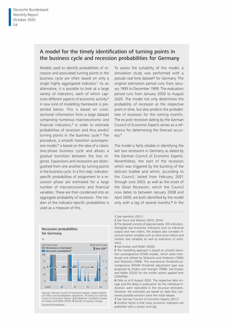
Models used to identify probabilities of re-cession and associated turning points in the business cycle are often based on only a single highly aggregated indicator.1 As an alternative, it is possible to look at a large variety of indicators, each of which cap-tures different aspects of economic activity.2 A new kind of modelling framework is pre-sented below. This is based on cross- sectional information from a large dataset comprising numerous macroeconomic and fi nancial indicators,3 in order to estimate probabilities of recession and thus predict turning points in the business cycle.4 The procedure, a smooth transition autoregres-sive model,5 is based on the idea of a classic two- phase business cycle and allows a gradual transition between the two re-gimes. Expansions and recessions are distin-guished from one another by turning points in the business cycle. In a fi rst step, indicator- specifi c probabilities of assignment to a re-cession phase are estimated for a large number of macroeconomic and fi nancial variables. These are then condensed into an aggregate probability of recession. The me-dian of the indicator- specifi c probabilities is used as a measure of this.

To assess the suitability of this model, a simulation study was performed with a pseudo real- time dataset6 for Germany. The original estimation period runs from Janu-ary 1993 to December 1999. The evaluation period runs from January 2000 to August 2020. The model not only determines the probability of recession at the respective point in time, but also predicts the probabil-ities of recession for the coming months. The ex post recession dating by the German Council of Economic Experts serves as a ref-erence for determining the forecast accur-acy.7

The model is fairly reliable in identifying the last two recessions in Germany as dated by the German Council of Economic Experts. Nevertheless, the start of the recession which was triggered by the bursting of the dotcom bubble and which, according to the Council, lasted from February 2001 through June 2003, as well as the onset of the Great Recession, which the Council now dates to between January 2008 and April 2009, are both identifi ed by the model only with a lag of several months.8 In the

Recession probabilities

for Germany

Sources: German Council of Economic Experts, Federal Statisti-

cal Office and Bundesbank calculations. 1 Dating by German

Council of Economic Experts. 2 Bundesbank calculations based

on Eraslan and Nöller (2020). 3 Quarter-on-quarter change.

Deutsche Bundesbank

2000 05 10 15 20

0

25

50

75

100

%

Recessions in Germany1

Recession probabilities2

– 10

– 5

0

+ 5

Real GDP 3Left-hand scale Right-hand scale

1 See Hamilton (2011).2 See Stock and Watson (2010, 2014).3 The dataset consists of approximately 100 indicators. Alongside real economic indicators such as industrial output and new orders, the analysis also considers fi -nancial market variables such as stock price indices and interest rate variables as well as indicators of senti-ment.4 See Eraslan and Nöller (2020).5 The modelling approach is based on smooth transi-tion autoregressive (STAR) models, which were intro-duced and refi ned by Teräsvirta and Anderson (1992) and Teräsvirta (1994). The momentum threshold au-toregressive (MTAR) threshold adjustment type was proposed by Enders and Granger (1998). See Eraslan and Nöller (2020) for the model variant applied here (ST/ MTAR).6 Data as at 8 August 2020. The respective data vin-tage and the delay in publication for the individual in-dicators were replicated in the recursive estimates. However, the estimates are based on data that con-tained possible revisions since the initial release.7 See German Council of Economic Experts (2017).8 Another factor is that many economic indicators are published with a certain time lag.


these cases.41 An above average rate of infla-

tion is also associated with a heightened prob-

ability of a cyclical peak in the following quar-

ter. The sign of the effect of house and equity

prices as well as outstanding loans – each

measured as deviations from their growth

trends – is highly dependent on their lag. In

addition, lagged values for the selected vari-

ables significantly improve the informative

value of the model, even if they have no statis-

tically significant impact on the probability that

a cyclical peak will occur when viewed in isol-

ation.

In some cases, the regression coefficients vary

greatly depending on the way in which cyclical

peaks are identified, the selection of explana-

tory variables, the underlying group of coun-

tries, and the forecast horizon. One reason for

this may be that many indicators contain simi-

lar information on imminent cyclical turning

points. Country- specific regressions largely con-

firm the impression that the duration of the up-

swing and the interest rate spread are good

predictors of imminent cyclical peaks. For peaks

that are followed by recessions, this holds true

for the interest rate spread. In this context, it

should also be noted that the coefficients only

reflect historical correlation patterns. These are

likely to contain indications of the driving forces

behind cyclical turnarounds. For example, the

1973 oil crisis can also be interpreted as a cause

of the subsequent downturn. By contrast, fi-

nancial market variables as well as survey- based

indicators probably only react in the run- up to

cyclical slumps because market participants

and respondents anticipate a downturn in

many cases. Furthermore, the possibility that

uncaptured factors are significant for the oc-

currence of cyclical peaks cannot be ruled out.

For these reasons, the statistical impact of indi-

Results should be interpreted with caution

fi rst case, the model pinpoints the start of the recession four months later, as May 2001 (and the end as early as March 2002). In the second case, the median nowcast in-dicates a recessionary phase from July 2008 to July 2009, i.e. with a time lag of six months (start of recession) and three months (end of recession). In this compari-son, however, it should be noted that these recessionary phases were not dated until a much later point in time. At the time of the recessions, the assessment was nowhere near as clear. This was particularly true of the Great Recession of 2008-09, the start of which often went undetected until later. By comparison, the model would have de-livered an early warning. Furthermore, for the downturn from 2001 to 2003 the model pointed to a dramatically rising risk of recession as early as March 2001, with a nowcast of 10% as well as forecasts of al-most 50% for April and nearly 80% for May.

The model gave warning signals more re-cently, too. In the second half of 2019, it indicated elevated recessionary risks, which then declined sharply at the beginning of 2020, however, owing to positive macro-economic data for January and February. At the current end, the estimated probability of recession did not increase until early May, but then did so abruptly, surging to 100%. However, the sweeping measures taken to contain the coronavirus pandemic were already being introduced in March. It was immediately clear that this would inev-itably result in a slump in economic activity. In this case, the delay in signalling a reces-sion was due to the fact that the model – unlike business cycle analysts – was un-able to take into account the economic im-pact of the measures until early May, when the macroeconomic indicators for March were released. This illustrates once again the special nature of the current crisis.

41 In the case of upswings that end in recessions, the rela-tionship between the duration of the upswing and the probability that a cyclical peak will occur is weaker than for upswings that transition into soft patches. This is consistent with the results of the survival analysis.


October 2020 55

vidual variables must be interpreted with cau-

tion.

Forecasting economic downturns

A key factor in predicting economic downturns

is the model’s forecast of the probability of an

upturn coming to an end. This probability tends

to rise sharply before soft patches, but espe-

cially before recessions. For example, models

indicated that the upswing prior to the global

financial and economic crisis was increasingly

fragile for almost all major advanced econ-

omies. Flat yield curves, high levels of private

debt and falling equity prices, but also the

above average duration of the upswing so far,

indicated a turning point ahead. Even clearer

fluctuations were seen in the probabilities of

recession for the United States at the turn of

the millennium (i.e. before the economic slump

triggered by the bursting of the dotcom bub-

ble) and in Japan in the run- up to the severe

economic crisis in the early 1990s.

The binary regressions therefore appear to pro-

vide valuable information about approaching

peaks and impending downturns. To assess the

quality of a forecast model more accurately, its

predictions are usually compared with events

that have actually occurred. This involves deriv-

ing warning signals from the forecast model

probabilities and comparing them with the ac-

tual cyclical turning points. To this end, a

threshold is sought which, when exceeded,

means that the forecast probability sends the

most reliable signal possible for a forthcoming

downturn. If it is set too high, potential signals

for downturns are missed. If it is set too low, a

high proportion of false signals is to be ex-

pected. For peaks that mark the beginning of

soft patches as well as those that are followed

by deep recessions, threshold optimisation

techniques suggest setting the threshold for

sending a signal at 8%.42

Beginning with the broad definition of a turn-

ing point, for this threshold, the model cor-

rectly classifies just over three- quarters of all

observations into those with and without

peaks. The error rate is only slightly higher

when looking exclusively at the peaks them-

selves. Only one- third failed to be identified.

However, in many cases, the model raises an

alarm where there was no turnaround in eco-

nomic activity. Nonetheless, it can be noted

Models indicate that upswings are usually increasingly fragile prior to crises

More accurate model evalu-ation hinges on establishing signals for recession

Although early warning signals are often also incorrect, …

Historical probabilities of cyclical peaks

in selected regions*

* Each estimation period begins with the first recorded probab-

ility. 1 Threshold value of 8%. Projected probabilities above

this threshold are interpreted as signalling a cyclical peak in the

respective quarter.

Deutsche Bundesbank

1970 75 80 85 90 95 00 05 10 15 20

0

20

40

%, quarterly data

0

20

40

60

80

Euro area

All peaks

Peaks followed by recessions

Threshold1

0

20

40

60

80

0

20

40

60

80

Japan

United States

United Kingdom

42 The information content of signals is established here by determining a ratio between the probability of a signal being triggered at a peak and the probability of a signal being a false alarm. To identify warning signals, it is more important to avoid type I errors (missed peaks). As a result, fairly low thresholds are therefore selected. See also Bussière and Fratzscher (2006).


that the probability of a peak is significantly

higher if the model sends a signal than if it

does not. Compared with a naive forecast,

which sets the unconditional probability of a

peak for each quarter, the model- based fore-

cast represents a clear improvement.

The binary regression model is even more in-

formative if the forecast is limited to recessions.

Here, almost all observations are identified cor-

rectly. The share of correctly identified peaks is

also significantly higher than in the previous

case. At the same time, however, the clear ma-

jority of the signals remain false. Nevertheless,

the model is considerably more informative

than naive forecasts. Although not every an-

nouncement was actually followed by a reces-

sion, the start of a recession was often clearly

signalled.43

The global economic slump in the first quarter

of 2020 can be used as a counterexample. Al-

though there were increasing signs of an immi-

nent soft patch in many countries last year, the

risk of a recession in the near future was con-

sidered to be low. Only in the United States did

the probability of recession rise slightly, owing

to a negative interest rate spread. The COVID-

19 pandemic itself and its consequences, how-

ever, could only be diagnosed, but not forecast

with a greater lead.

Summary

In summary, quantitative business cycle analysis

can be used to identify fragile macroeconomic

upturns and also to predict downturns. Reces-

sions, in particular, often appear to be signalled

in advance – at least when looked at with hind-

sight. All the same, it must be acknowledged

that the models presented here failed to recog-

nise a few (sometimes severe) downturns.

Turning points could even be missed more fre-

quently in day- to- day business cycle analysis,

not least because the characteristics of down-

turns often differ in their details from the pat-

terns observed in previous cycles. However, it is

precisely the particularities of the situation pre-

vailing at a given time that are not yet reflected

in the estimated forecast equations.

A look at the accuracy of judgements made by

experts confirms how challenging it can be to

predict economic downturns. In June 2008, for

example, the Bundesbank was still anticipating

fairly brisk growth in its forecasts for 2008 and

2009.44 Six months later, the outlook was for

… recessions, in particular, are frequently recognised in advance

Pandemic- related eco-nomic crisis unforecastable

Not all reces-sions can be predicted

Even profes-sional business cycle analysts are often sur-prised by crises

Accuracy of signals and associated probabilities of a cyclical peak

Threshold for sending a signal: 8%

Status

All peaks Peaks followed by recessions

No signal Signal Total No signal Signal Total

No peak 535 152 687 1,112 54 1,166Peak 17 32 49 5 21 26

Total 552 184 736 1,117 75 1,192

Proportion of correctly identifi ed observations 77.0% 95.1%

Proportion of correctly identifi ed peaks 65.3% 80.8%

Proportion of false signals 82.6% 72.0%

Unconditional probability of a peak 6.7% 2.2%

Probability of a peak if signal sent 17.4% 28.0%

Probability of a peak if no signal sent 3.1% 0.4%

Deutsche Bundesbank

43 In almost half of all cases, an increase in the probability of a turning point interpreted as a false signal was indeed followed by a recession after a few quarters. The forecast models would therefore have indicated that the upturn was highly fragile in these situations, too.44 See Deutsche Bundesbank (2008a).


October 2020 57

little growth in GDP over the course of 2009.45

However, the current data show that, in the

wake of the global financial and economic cri-

sis, German GDP fell markedly from as early as

the second quarter of 2008, decreasing by

3.3% over the course of 2009. Similarly, the

International Monetary Fund has seldom fore-

cast a decline in GDP in its published projec-

tions over the past 30 years. Even during crisis

periods, its assessments for the current year

were still too optimistic in around half of all

cases. Other national and international organ-

isations and private sector analysts have per-

formed similarly poorly in the past.46

Various explanatory approaches are put for-

ward for this patchy overall performance. Some

suggest that people generally tend to stick to

an assessment once it has been made and do

not initially assign enough importance to new

information that challenges it.47 It may also be

the case that a recession – especially one that

is less severe – is initially difficult to identify

from the preliminary data delivered by the eco-

nomic indicators. Macroeconomic forecasts

would therefore be adjusted too slowly, despite

signs of a deterioration in the situation. Other

explanations are based on the incentives for

business cycle forecasters. For instance, they

might be reluctant to predict a recession if mis-

judgements could potentially result in major

costs such as reputational damage.48 In add-

ition, the projections of international organisa-

tions might be influenced by political motives

or concerns that a pessimistic forecast could

become “self- fulfilling”.49 Finally, however, it is

also possible that the picture may be clouded

by the fact that, in some cases, impending

downturns are detected early on and prevented

by means of forward- looking economic policy

measures. Recessions avoided in this way

would not be included in the statistics.

Although these factors certainly play some-

thing of a role, there is still much to suggest

that, in the end, some downturns simply can-

not be predicted. Even economies that previ-

ously appeared to be fairly resilient can be

plunged into recession by shocks of sufficient

magnitude. The latest global economic crisis

resulting from the coronavirus pandemic under-

lines this once again. The fact that no warnings

of an imminent economic turnaround are is-

sued in situations like this should not therefore

be considered a failure on the part of the ex-

perts. Business cycle research can, however,

identify undesirable developments or potential

excesses and thus an increased risk of reces-

sion. Quantitative methods are an important

tool in this regard.

Explanatory approaches

Forecast models an important tool for identifying vulnerabilities

Accuracy of IMF recession forecasts*

Sources: IMF and Bundesbank calculations. * All forecasts for all countries and groups of countries from the April and Octo-ber editions of the World Economic Outlook since 1991 have been taken into consideration. The October edition for the fol-lowing year is used to determine GDP outcomes.

Deutsche Bundesbank

0

20

40

60

80

100

Percentage of correctly forecast GDP declines

Oct.Apr.Oct.Apr.Oct.Apr.Following yearCrisis yearPreceding year

Time of forecast

45 See Deutsche Bundesbank (2008b).46 For more information, see Loungani (2001) and An et al. (2018).47 This argument was first put forward by Nordhaus (1987).48 See Zellner (1986).49 For instance, an independent review of IMF forecasts published in the context of large support programmes found that assessments of the economic outlook were sys-temically overoptimistic. See Independent Evaluation Office of the International Monetary Fund (2014).


List of references

An, Z., J. T. Jalles and P. Loungani (2018), How well do economists forecast recessions?, Inter-

national Finance, Vol. 21 (2), pp. 100-121.

Andersson, M. and A. D’Agostino (2008), Are sectoral stock prices useful for predicting euro area

GDP?, ECB Working Paper Series, No 876.

Bauer, M. D. and T. M. Mertens (2018), Economic Forecasts with the Yield Curve, FRBSF Economic

Letter, No 7.

Baxter, M. and M. A. Kouparitsas (2005), Determinants of business cycle comovement: A robust

analysis, Journal of Monetary Economics, Vol. 52 (1), pp. 113-157.

Boissay, F., F. Collard and F. Smets (2016), Booms and Banking Crises, Journal of Political Economy,

Vol. 124 (2), pp. 489-538.

Borio, C., M. Drehmann and D. Xia (2019), Predicting recessions: financial cycle versus term spread,

BIS Working Paper, No 818.

Brock, W. A. and L.J. Mirman (1972), Optimal Economic Growth And Uncertainty: The Discounted

Case, Journal of Economic Theory, Vol. 4 (3), pp. 479-513.

Bry, G. and C. Boschan (1971), Cyclical Analysis of Time Series: Selected Procedures and Computer

Programs, National Bureau of Economic Research, New York.

Burns, A. F. and W. C. Mitchell (1946), Measuring Business Cycles, National Bureau of Economic

Research, New York.

Burnside, C. (1998), Detrending and business cycle facts: A comment, Journal of Monetary Eco-

nomics, Vol. 41 (3), pp. 513-532.

Bussière, M. and M. Fratzscher (2006), Towards a new early warning system of financial crises,

Journal of International Money and Finance, Vol. 25 (6), pp. 953-973.

Canova, F. (1998), Detrending and business cycle facts, Journal of Monetary Economics, Vol. 41

(3), pp. 475-512.

Carare, A. and A. Mody (2012), Spillovers of Domestic Shocks: Will They Counteract the ‘Great

Moderation’?, International Finance, Vol. 15 (1), pp. 69-97.

Carstensen, K., M. Heinrich, M. Reif and M. H. Wolters (2020), Predicting ordinary and severe

recessions with a three- state Markov- switching dynamic factor model: An application to the Ger-

man business cycle, International Journal of Forecasting, Vol. 36 (3), pp. 829-850.

Castro, V. (2010), The duration of economic expansions and recessions: More than duration

dependence , Journal of Macroeconomics, Vol. 32 (1), pp. 347-365.


October 2020 59

Centre for Economic Policy Research (2020), Chronology of Euro Area Business Cycles, https://

eabcn.org/dc/chronology-euro area-business-cycles, accessed on 10 August 2020.

Centre for Economic Policy Research (2012), Euro Area Business Cycle Dating Committee: Meth-

odological note, https://cepr.org/Data/Dating/Dating-Methodology-Nov-2012.pdf, accessed on

19 October 2020.

Centre for Economic Policy Research (2003), Dating Committee Findings 22 September 2003,

https://cepr.org/PRESS/Dating-Committee-Findings-22-September-2003.pdf, accessed on 12 Oc-

tober 2020.

Cleves, M., W. Gould, R. Gutierrez and Y. Marchenko (2008), An Introduction to Survival Analysis

using Stata, 2nd edition, Stata Press, College Station, TX.

Deutsche Bundesbank (2014), Real economic adjustment processes and reform measures, Monthly

Report, January 2014, pp. 19-37.

Deutsche Bundesbank (2010), Constructing a new leading indicator for the global economy,

Monthly Report, May 2010, pp. 18-19.

Deutsche Bundesbank (2008a), Outlook for the German economy: macroeconomic projections for

2008 and 2009, Monthly Report, June 2008, pp. 17-30.

Deutsche Bundesbank (2008b), Outlook for the German economy: macroeconomic projections for

2009 and 2010, Monthly Report, December 2008, pp. 17-29.

Diebold, F. X. and G. D. Rudebusch (1990), A Nonparametric Investigation of Duration Dependence

in the American Business Cycle, Journal of Political Economy, Vol. 98 (3), pp. 596-616.

Enders, W. and C. W. J. Granger (1998), Unit- Root Tests and Asymmetric Adjustment With an

Example Using the Term Structure of Interest Rates, Journal of Business & Economic Statistics,

Vol. 16 (3), pp. 304-311.

Eraslan, S. and M. Nöller (2020), Recession probabilities falling from the STARs, Deutsche Bundes-

bank Discussion Paper, No 08/ 2020.

Estrella, A. and F. S. Mishkin (1998), Predicting U.S. Recessions: Financial Variables as Leading Indi-

cators, The Review of Economics and Statistics, Vol. 80 (1), pp. 45-61.

Estrella, A. and F. S. Mishkin (1997), The predictive power of the term structure of interest rates in

Europe and the United States: Implications for the European Central Bank, European Economic

Review, Vol. 41 (7), pp. 1375-1401.

European Central Bank (2019), Characterising the current expansion across non- euro area ad-

vanced economies: where do we go from here?, Economic Bulletin, 2/ 2019, pp. 39-43.

Fagan, G., J. Henry and R. Mestre (2005), An area- wide model for the euro area, Economic Mod-

elling, Vol. 22 (1), pp. 39-59.


https://eabcn.org/dc/chronology-euro-area-business-cycles

https://eabcn.org/dc/chronology-euro-area-business-cycles

https://cepr.org/Data/Dating/Dating-Methodology-Nov-2012.pdf

https://cepr.org/PRESS/Dating-Committee-Findings-22-September-2003.pdf

Fornari, F. and W. Lemke (2010), Predicting recession probabilities with financial variables over

multiple horizons, ECB Working Paper Series, No 1255.

Frisch, R. (1933), Propagation problems and impulse problems in dynamic economics, in Economic

Essays in Honour of Gustav Cassel, Allen & Unwin, London.

German Council of Economic Experts (2017), Konjunkturzyklen der deutschen Volkswirtschaft,

Annual Economic Report 2017/ 18: Für eine zukunftsorientierte Wirtschaftspolitik (Towards a

forward- looking economic policy), November 2017, pp. 134-135.

Goodfriend, M. and R.G. King (2005), The incredible Volcker disinflation, Journal of Monetary Eco-

nomics, Vol. 52 (5), pp. 981-1015.

Gorton, G. and G. Ordoñez (2014), Collateral Crises, American Economic Review, Vol. 104 (2),

pp. 343-378.

Grigoraş, V. and I.E. Stanciu (2016), New evidence on the (de)synchronisation of business cycles:

Reshaping the European business cycle, International Economics, Vol. 147, pp. 27-52.

Hamilton, J. D. (2018), Why You Should Never Use the Hodrick- Prescott Filter, The Review of Eco-

nomics and Statistics, Vol. 100 (5), pp. 831-843.

Hamilton, J. D. (2011), Calling recessions in real time, International Journal of Forecasting, Vol. 27

(4), pp. 1006-1026.

Harding, D. and A. Pagan (2002), Dissecting the cycle: a methodological investigation, Journal of

Monetary Economics, Vol. 49 (2), pp. 365-381.

Heimberger, P. (2017), Did fiscal consolidation cause the double- dip recession in the euro area?,

Review of Keynesian Economics, Vol. 5 (3), pp. 439-458.

Hodrick, R. J. (2020), An Exploration of Trend- Cycle Decomposition Methodologies in Simulated

Data, NBER Working Paper, No 26750.

Hodrick, R. J. and E. C. Prescott (1997), Postwar U.S. Business Cycles: An Empirical Investigation,

Journal of Money, Credit and Banking, 29 (1), pp. 1-16.

Hoffmann, M., M. Kliem, M. Krause, S. Moyen and R. Sauer (2020), Rebalancing the euro area: Is

wage adjustment in Germany the answer?, Deutsche Bundesbank Discussion Paper, No 17/ 2020.

Independent Evaluation Office of the International Monetary Fund (2014), IMF Forecasts: Process,

Quality, and Country Perspectives, Evaluation Report.

Kilian, L. and R. J. Vigfusson (2017), The Role of Oil Price Shocks in Causing U.S. Recessions, Journal

of Money, Credit and Banking, Vol. 49 (8), pp. 1747-1776.

Kose, M. A., C. Otrok and C. H. Whiteman (2008), Understanding the evolution of world business

cycles, Journal of International Economics, Vol. 75 (1), pp. 110-130.


October 2020 61

Kose, M. A., C. Otrok and C. H. Whiteman (2003), International Business Cycles: World, Region,

and Country- Specific Factors, American Economic Review, Vol. 93 (4), pp. 1216-1239.

Kydland, F. E. and E. C. Prescott (1982), Time to Build and Aggregate Fluctuations, Econometrica,

Vol. 50 (6), pp. 1345-1370.

Lancaster, T. (1992), The Econometric Analysis of Transition Data, Econometric Society Mono-

graphs, No 17, Cambridge University Press.

Loungani, P. (2001), How accurate are private sector forecasts? Cross- country evidence from con-

sensus forecasts of output growth, International Journal of Forecasting, Vol. 17 (3), pp. 419-432.

Lucas, R. E. (1972), Expectations and the Neutrality of Money, Journal of Economic Theory, Vol. 4

(2), pp. 103-124.

Mills, L. (1988), Can Stock Prices Reliably Predict Recessions?, Business Review, Federal Reserve

Bank of Philadelphia, pp. 3-14.

National Bureau of Economic Research (2020a), The NBER’s Recession Dating Procedure, https://

www.nber.org/cycles/recessions.pdf, accessed on 15 September 2020.

National Bureau of Economic Research (2020b), US Business Cycle Expansions and Contractions,

https://www.nber.org/cycles.html, accessed on 10 August 2020.

Ng, E. C. Y. (2010), Production fragmentation and business- cycle comovement, Journal of Inter-

national Economics, Vol. 82 (1), pp. 1-14.

Nilsson, R. and G. Gyomai (2011), Cycle Extraction: A Comparison of the Phase- Average Trend

Method, the Hodrick- Prescott and Christiano- Fitzgerald Filters, OECD Statistics Working Papers,

No 2011/ 04.

Nordhaus, W. (1987), Forecasting Efficiency: Concepts and Applications, The Review of Economics

and Statistics, Vol. 69 (4), pp. 667-674.

OECD (2020), OECD Economic Outlook, Vol. 2020 (1), OECD Publishing, Paris.

Orphanides, A. and S. van Norden (2002), The Unreliability of Output- Gap Estimates in Real Time,

The Review of Economics and Statistics, Vol. 84 (4), pp. 569-583.

Paul, P. (2020), A macroeconomic model with occasional financial crises, Journal of Economic Dy-

namics and Control, Vol. 112, pp. 1-21.

Rudebusch, G.D. (2016), Will the Economic Recovery Die of Old Age?, FRBSF Economic Letter,

No 2016-03.

Rudebusch, G.D. and J.C. Williams (2009), Forecasting Recessions: The Puzzle of the Enduring

Power of the Yield Curve, Journal of Business & Economic Statistics, Vol. 27 (4), pp. 492-503.


https://www.nber.org/cycles/recessions.pdf

https://www.nber.org/cycles/recessions.pdf

https://www.nber.org/cycles.html

Slutzky, E. (1937), The Summation of Random Causes as the Source of Cyclic Processes, Economet-

rica, Vol. 5 (2), pp. 105-146.

Stock, J. H. and M. W. Watson (2014), Estimating turning points using large data sets, Journal of

Econometrics, Vol. 178 (2), pp. 368-381.

Stock, J. H. and M. W. Watson (2010), Indicators for Dating Business Cycles: Cross- History Selection

and Comparisons, American Economic Review, Vol. 100 (2), pp. 16-19.

Stock, J. H. and M. W. Watson (2005), Understanding Changes in International Business Cycle Dy-

namics, Journal of the European Economic Association, Vol. 3 (5), pp. 968-1006.

Teräsvirta, T. (1994), Specification, Estimation, and Evaluation of Smooth Transition Autoregressive

Models, Journal of the American Statistical Association, Vol. 89 (425), pp. 208-218.

Teräsvirta, T. and H. M. Anderson (1992), Characterizing Nonlinearities in Business Cycles Using

Smooth Transition Autoregressive Models, Journal of Applied Econometrics, Vol. 7 (1), pp. 119-136.

Tian, R. and G. Shen (2019), Predictive power of Markovian models: Evidence from US recession

forecasting, Journal of Forecasting, Vol. 38 (6), pp. 525-551.

Zarnowitz, V. and A. Ozyildirim (2006), Time series decomposition and measurement of business

cycles, trends and growth cycles, Journal of Monetary Economics, Vol. 53 (7), pp. 1717-1739.

Zellner, A. (1986), Biased predictors, rationality and the evaluation of forecasts, Economics Letters,

Vol. 21 (1), pp. 45-48.

The tables accompanying this article are printed on pp. 64 f.


October 2020 63

Regression table for forecasting cyclical peaks over various time horizons (all peaks)o

Item(1)Peak in t+1

(2)Peak in t+25

(3)Peak in t+35

(4)Peak in t+45

(5)Peak in t+1to t+4

Duration 0.094** 0.100** 0.095** 0.093** 0.096**(0.046) (0.042) (0.038) (0.041) (0.047)

Interest rate spreadt1 – 0.405*** – 0.213* – 0.127 – 0.135 – 0.269*

(0.113) (0.128) (0.165) (0.165) (0.143)

Equity price indext2 – 0.044 – 0.014 0.013 0.013 – 0.009

(0.032) (0.023) (0.028) (0.035) (0.012)

Industry sentimentt 0.069*** 0.032 0.002 0.024 0.036**(0.018) (0.034) (0.032) (0.033) (0.014)

Industry sentimentt–1 – 0.031** – 0.003 0.021 – 0.001 – 0.006(0.015) (0.036) (0.033) (0.030) (0.014)

Consumer sentimentt – 0.082* – 0.058 – 0.030 0.084** – 0.013(0.045) (0.047) (0.026) (0.042) (0.036)

Consumer sentimentt–1 0.083** 0.086*** 0.079*** – 0.036 0.044*(0.038) (0.031) (0.026) (0.036) (0.025)

GDP defl atort2 – 0.183 – 0.231 – 0.282 0.136 – 0.107

(0.175) (0.329) (0.236) (0.361) (0.256)

GDP defl atort–12 – 0.275 – 0.155 0.205 0.132 0.043

(0.323) (0.222) (0.327) (0.162) (0.211)

Credit- to- GDPt3 0.045*** 0.052*** 0.054*** 0.052*** 0.063***

(0.014) (0.010) (0.009) (0.010) (0.012)

House price indext4 – 0.021*** – 0.022*** – 0.021*** – 0.022*** – 0.027***

(0.005) (0.005) (0.005) (0.006) (0.006)

Constant – 3.320*** – 3.443*** – 3.438*** – 3.577*** – 1.741**(0.900) (0.875) (0.809) (0.840) (0.848)

Countries 9 9 9 9 9

Country dummies Yes Yes Yes Yes Yes

Observations 736 734 732 729 736

McFadden’s adjusted R2 0.042 0.011 0.009 0.009 0.099

o Robust and clustered standard errors shown in parentheses: *** p < 0.01, ** p < 0.05, * p < 0.1. 1 Difference between long- term and short- term interest rates. 2 Rate of change over preceding quarter. 3 Deviation from linear trend. 4 Deviation from log- linear trend. 5 Assuming that an upturn continues until that point in time.

Deutsche Bundesbank


Regression table for forecasting cyclical peaks over various time horizons (only peaks followed by recessions)o

Item(1)Peak in t+1

(2)Peak in t+25

(3)Peak in t+35

(4)Peak in t+45

(5)Peak in t+1 to t+4

Duration 0.042** 0.036** 0.020 0.024 0.029*(0.017) (0.017) (0.016) (0.016) (0.015)

Interest rate spreadt1 – 1.614*** – 1.438*** 0.054 – 0.427 – 0.767***

(0.450) (0.349) (0.346) (0.371) (0.104)

Interest rate spreadt-11 0.521*** 1.199*** – 0.668 – 0.274 0.124

(0.198) (0.363) (0.579) (0.873) (0.183)

Interest rate spreadt-21 0.339 – 0.296 0.332 0.374 0.134

(0.415) (0.453) (0.308) (0.755) (0.279)

GDP defl atort2 0.673* 1.166** 0.432 0.244 0.564**

(0.353) (0.500) (0.360) (0.223) (0.276)

GDP defl atort-12 0.856* 0.198 0.385** 0.061 0.331

(0.497) (0.431) (0.176) (0.362) (0.232)

GDP defl atort-22 0.207 0.114 – 0.032 0.579*** 0.350

(0.290) (0.187) (0.286) (0.154) (0.216)

House price indext3 – 0.070 0.179 – 0.025 0.198*** 0.050

(0.072) (0.138) (0.113) (0.073) (0.050)

House price indext-13 0.222* – 0.254 0.212 – 0.206 0.026

(0.119) (0.247) (0.199) (0.133) (0.051)

House price indext-23 – 0.112 0.110 – 0.160* 0.034 – 0.047

(0.104) (0.130) (0.091) (0.070) (0.034)

Credit-to-GDPt4 0.031 0.498*** 0.083 0.016 0.169**

(0.138) (0.124) (0.076) (0.095) (0.082)

Credit-to-GDPt-14 0.561*** – 0.584** 0.031 0.119 0.005

(0.162) (0.232) (0.084) (0.151) (0.063)

Credit-to-GDPt-24 – 0.688*** 0.007 – 0.183* – 0.200*** – 0.242***

(0.241) (0.177) (0.101) (0.073) (0.069)

Equity price indext3 – 5.505 – 5.040* 2.849 2.221 – 0.357

(4.591) (2.728) (3.228) (4.995) (1.727)

Equity price indext-13 2.039 5.930 – 1.492 0.803 0.807

(8.054) (4.794) (5.548) (7.835) (1.250)

Equity price indext-23 6.084 1.870 1.346 – 0.153 2.311

(4.068) (4.054) (4.543) (3.208) (1.505)

Oil pricet3 0.038*** 0.012 0.001 0.006 0.012***

(0.009) (0.016) (0.010) (0.019) (0.004)

Oil pricet-13 – 0.014 0.000 0.006 – 0.006 – 0.005

(0.018) (0.013) (0.018) (0.015) (0.006)

Oil pricet-23 0.029** 0.001 – 0.016 0.014 0.002

(0.014) (0.024) (0.020) (0.012) (0.010)

Constant – 11.329*** – 9.899*** – 7.382*** – 8.016*** – 7.232***(2.973) (2.539) (2.062) (2.036) (2.013)

Countries 9 9 9 9 9

Country dummies Yes Yes Yes Yes Yes

Observations 1,192 1,187 1,182 1,147 1,192

McFadden’s adjusted R2 0.195 0.101 – 0.044 – 0.029 0.227

o Robust and clustered standard errors shown in parentheses: *** p < 0.01, ** p < 0.05, * p < 0.1. 1 Difference between long- term and short- term interest rates. 2 Rate of change over preceding quarter. 3 Deviation from log- linear trend. 4 Deviation from linear trend. 5 Assuming that an upturn continues until that point in time.

Deutsche Bundesbank


October 2020 65

patterns of international business cycles - october 2020

Documents