This PDF is a selection from an out-of-print volume from the National Bureau of Economic Research

Volume Title: Consumption and Business Fluctuations: A Case Study of the Shoe, Leather, Hide Sequence

Volume Author/Editor: Ruth P. Mack

Volume Publisher: NBER

Volume ISBN: 0-870-14090-6

Volume URL: http://www.nber.org/books/mack56-1

Publication Date: 1956

Chapter Title: Patterns in Consumer Purchases of Shoes

Chapter Author: Ruth P. Mack

Chapter URL: http://www.nber.org/chapters/c4800

Chapter pages in book: (p. 44 - 59)

CHAPTER 5

PATTERNS IN CONSUMER PURCHASES OF. SHOES

Could we precisely define a shoe, a purchase, and aconsumer, then during each month of each year, thenumber of shoes purchased by consumers would bean exact quantity; could we also define purchase price,then the number of dollars expended for shoes wouldsimilarly be an exact quantity. Change in theseamounts during business cycles and its cause is thesubject of this chapter.

But unfortunately the real subject is never encoun-tered. We have no direct experience of aggregate shoesales. The figure must be reconstructed from fragmen-tary evidence, and we can actually speak only of thisconstruct. In the course of months and years of workwith the efilgy, one slips inevitably at times into regard-ing its papier-mâché as flesh and bone. All the morereason to build it with the utmost care.

DOLLAR SALES

Estimates of Retail Shoe Sales

Sufficient information on retail shoe sales is availableto provide the basis for monthly estimates beginning inJanuary 1926. How the estimates were made is de-scribed in a technical paper on the factors determiningconsumer shoe buying.' Some of the problems thatwere encountered are discussed, and an attempt ismade to evaluate the results. Very briefly, the estimateswere constructed in the following way.

Because additional material became available in1935, the first ten years of the series (1926—1935) wereconstructed in a somewhat different manner from therest. The basic data used in the first segment were: (1)sales of shoe departments of department stores col-lected by the seven Federal Reserve Banks of Boston,New York, Richmond, Cleveland, Chicago, Dallas, andSan Francisco; (2) sales of six local independent andchain shoe-store organizations collected by the FederalReserve Bank of Philadelphia; (3) sales of five largenational shoe chains reported to the Federal ReserveBank of New York; and (4) sales of one large nationalshoe chain made available directly to the NationalBureau of Economic Research. These series wereweighted for the relative importance in total shoe

1 Ruth P. Mack, Factors Influencing Consumption: An Ex-periinental Analysis of Shoe Buying, National Bureau of Eco-nomic Research, Technical Paper 10, 1954.

sales of the section of the country or type of distribu-tion, or both, and combined in a single index.

Study of the index indicated that the cyclical move-ments of these data were probably reasonably repre-sentative of shoe sales in general. However, the long-run trend certainly was not. Accordingly, the trend ofthe index was adjusted to the trend of another estimateof retail shoe sales, one that was more reliable as totrend though not as to shortrun movements. For thispurpose, estimates of annual total shoe sales were con-structed for 1926 to 1941 on the basis of monthly censusstatistics on shoe production, adjusted for net exportsof shoes and changes in distributors' inventories (thelatter figures were based on inventory statistics of shoe-departments in department stores and of shoe whole-salers); the resulting annual figures (1926-1940) forthe number of pairs of shoes sold at retail were con-verted to dollar values by means of an index of the-average retail selling price for all shoes sold eachyear.2 The ratio was then computed between these an-•nual estimates of total shoe sales and the index ofof shoe chains and shoe departments; a straight-linetrend was fitted to the logarithms of the ratios, and ourshoe-sales index multiplied by the ordinates of this.trend.

The estimates for the later segment (after 1935)were based on the National Bureau's department-store'-data for shoe departments and statistics on independ-ent and chain shoe stores collected by the Departmentof Commerce.3 The department-store, chain-store, and'.independent-store statistics were weighted by their -relative importance in total shoe sales and used with-out a trend adjustment. The index was linked to dollarestimates of aggregate sales of shoes by retailin 1939; it was based on information from both theCensus of Manufactures and the Census of Distribu-.tion in that year. The earlier segment was linked to the--later one in 1935.

Seasonal adjustments were made for each component:of the index—each Federal Reserve district for the de-.partment store data, and for both the chain-store and,.independent-store indexes. In addition to the adjust-

2 The index is discussed in the next section.About 100 independent shoe stores and 25 chain organiza-..

tions reported to the Department in 1986, and the number in- -'creased in subsequent years.

CONSUMER PURCHASES 45

ment for usual monthly patterns of sales, correctionswere also made for the changing date of Easter andalso for the varying number of Saturdays and Sundaysin each month.

How closely the estimates achieve the actual valuestoward which they grope is difficult to say. The earlierfigures, particularly those before 1929, are less surethan the later ones. On the whole, it seems probablethat the figures give a respectable reproduction offluctuations in shoe sales, though major ones are morelikely to be damped than exaggerated. The generallevels of the estimates ought not to be greatly in error.4

SHOE PRICES AND SALES IN PHYSICAL UNITS

In addition to a record of the number of dollars thatconsumers spend on shoes, it is desirable for manypurposes to have a record of purchases in physicalunits. Direct information of this sort is not available.It is necessary, therefore, to divide the dollar estimatesby a suitable price index. Such an index might aim ata physical volume measure that is a simple count ofall pairs of shoes sold each month, whether open-toedsandal, high work shoe, or street oxford. Alternatively,if a popular-priced open-toed sandal is judged to incor-porate markedly less worth than a fine calf oxford, itmight seem preferable to convert the number of pairssold into some sort of standardized pair, calling, for ex-ample, twenty sandals equivalent to ten oxfords.

The first sort of measure is necessary in order to com-pare sales at retail with shoe production, since pro-duction statistics are obtained directly from shoe manu-facturers in the form of a simple count of the numberof leather or part-leather shoes turned out. Moreover,the number of things called a pair of shoes that peoplebuy each month or year in the United States has directmeaning and interest in many contexts. But the secondconcept has uses too. Ideally, it would record changesin purchased shoe utility by converting the utility ofthe pairs actually sold into fractions or multiples ofthe utility offered by some standard shoe. Actually, ofcourse, only prices, not utilities, can be compared, andthe relationship between relative price and relativeutility is highly obscure. Accordingly, all one can dois to aim to measure shoe sales in "standardized pairs,"where the process of standardization simply endeavorsto convert a measure of change in the sorts of shoesselected to change in the number of a standard com-bination of shoes of a standard quality; another namefor such a series is shoe sales in constant prices.5 Incontrast, for the first physical volume measure—shoe

See the last section of the appendix in Mack, op. cit., forthe development of these evaluations.

Geoffrey Moore has indicated the precise meaning of these

sales in actual pairs—changes in the sorts of se-lected is accepted without evaluation.

In actuality, how close it is possible to come to thetwo concepts of the physical volume of shoe sales de-pends on how closely the available price arid salesstatistics approach those theoretically necessary. And,of course, they fall very wide of the mark. For the mostpart, available statistics on the shoe prices aim to re-cord the price of a shoe of unchanged quality. But in-stead of covering all or a representative sample of shoesthat may have had different price histories or thangedtheir relative importance in total production, they ofnecessity apply to only a few staple sorts shoes.Starting in 1923, the National Industrial ConferenceBoard has collected monthly statistics from severalhundred stores, first for two sorts of shoes and later forfour. We are greatly indebted to the Conference Boardfor maldng these unpublished statistics available. TheBureau of Labor Statistics has collected informationfrom several stores in each of thirty-four cities forabout a dozen shoes, starting in 1935. Figures fromthese two sources have been combined to obtain anindex of shoe prices. When dollar sales are bythe price index, an index of sales in standardized pairs(or alternately, in constant prices) is obtained, In ad-dition to their paucity, the actual data diverge seriously

several concepts of shoe sales and their bearing on the informa-tion about prices and quantities that they require or imply:

(1) Actual pairs = = sales in year 1average price in year 1

Index, year 0 as base =

In constant prices =

(3) Standardized pairs =

Expressions 2 and 3 are equal, both being:

Sales in year 1Price index using year 1 weights

± average price in year 0

Index, year 0 as base = ( Laspeyres index)

(4) Available estimates of shoe sales in constant shoe dollars =

Index, year 0 as base index)

(2)

I.-_...-.-. - —.—

I

46 CHAPTER 5

from those theoretically required and the deficienciesneed to be borne in mind when working with the fig-ures. The statistics apply to staple shoes, and stapleshoes may respond to cyclical influences somewhat dif-ferently from the high-style shoes now so popular.Also, markdowns or special sales are specifically ex-cluded from the basic reports, and markdowns aresubstantially more important in years of poor than inyears of good business. These and other difficultiesprobably have the net effect of understating cyclicalfluctuation in shoe prices and consequently overstatingfluctuation in sales of standardized pairs.

To construct the first type of physical volume meas-ure a price series for the average price at which shoeswere actually sold was needed—a record of averagesales price. Such a figure for wholesale markets may bebased on the biennial Census of Manufactures forevery other year from 1927 to 1939 inclusive. TheCensus of Manufactures figures were converted to anaverage retail sales price by raising them by the typicalmargin between retail and factory price of 41 per centof retail price (or 69.5 per cent of factory price)Values between the biennial bench-marks were inter-polated by the monthly shoe price index. At least someof the shortcomings of this series are obvious: the main-tained markup for distribution is not fixed from year toyear, but is dependent on business conditions; yet in-formation is not adequate to determine the proper an-nual figures. Further, the monthly estimates are boundto be seriously in error during periods when consider-able trading up or trading down is taking place, for thissort of change is not reflected in the interpolatingseries. Fortunately it was possible to compare thisseries with ones of similar principle obtained fromtwo large shoe-chain organizations, and they werefound to be in welcome agreement.

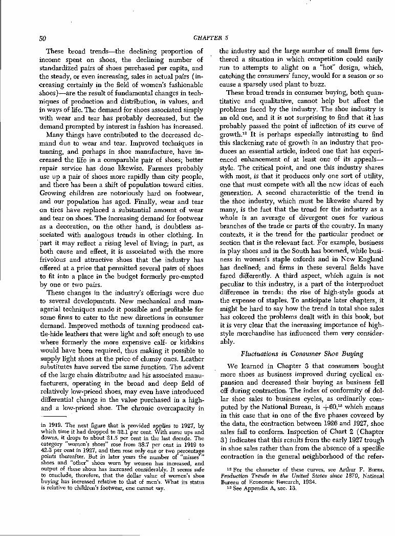
The three measures of shoe sales are displayed inChart 7. It is worthwhile to view carefully the dif-ference between the two types of deflated data sincethis represents the aspect of typical retail and produc-tion statistics that is merely a function of usual dif-ferences in how retailers and producers ordinarily re-port the flow of goods. Sales in actual pairs resemblethe sort of physical measure found in many statisticson production. Sales in standardized pairs, on the otherhand, is a sample of the genus "sales in constantprices," the use of which is so common in recordingconsumer takings in "real" terms. By using whicheverof the three measures seems appropriate in context,trends and cyclical characteristics of consumer buyingof footwear may be examined.

8 If the margin is 41 per cent of the retail price X, then it is(0.41X x 100)/(X — 0.41X) per cent, or 69.5 per cent, of thefactory price (IC — 0.41X).

Trends in Shoe Sales

Table 13 presents annual estimates that show thebroad changes over the years in the American con-sumer's expenditure on shoes. There was a fall in shoebuying, measured either in current or constant prices(columns 1 and 5), between the two peak years 1929and 1937, but a reversal of the downward trend, evenmeasured in constant prices, tqok place during WorldWar II. Information from the Census of Manufacturescan be used to push the picture backward, and incolumn 2 or 6 of the table we see that the peak year of1923 was still higher than 1929. Before World War I,however, dollar shoe sales seem to have been subject toan upward trend, and the reversal came some time dur-ing or after the war, though this was not apparentwhen changes in price were allowed for (column 6).For the stretch between World Wars I and II, in anyevent, shoe sales in either current or constant pricessuffered a trend decline.

Since the population of the country has increased,and since the need for shoes is affected by the numberof feet to be shod, the downward trend in standardizedpairs purchased by the average person is stronger thanthe aggregate figures show. Per capita purchases inconstant prices (last column) declined at the rate ofabout 2.6 per cent of its average value during the inter-war

The downward trend in shoe buying might havebeen associated with a downward trend in all con-sumer buying or in consumer income. But per capitaincome adjusted for change in the cost of living did notdecrease; on the contrary, it increased, at least in thetwenties.8 Consequently, shoe sales (adjusted forchange in the price of staple shoes) must have pre-empted a decreasing portion of the consumer "rear'dollar. This was also true when both sets of figureswere compared without the price adjustments: theper cent of disposable consumer income spent for shoeswas 2.09 in 1926, 2.08 in 1929, 1.86 in 1937, 1.67 in1941, and 1.43 in 1948, all years of more or less peakactivity. The rise in real income before 1929 and after1941 would normally be associated with a drop in theproportion of income spent on shoes. At relativelyhigh levels of income, a smaller proportion of incomeis ordinarily spent on all purchases (a larger propor-tion saved). Also, since shoes are a more necessary

A straight-line trend was fitted to the production data incolumn 9 for 1919 through 1939. The equation was y = $7.063— $01857 per year (counting from 1929). The average percapita output for the period was $7.06 in 1935—1939 (whole-sale) shoe prices, and $01857 is 2.6 per cent of $7.06.

8 See Simon Kuznets, National Income and Its Composition,1919—1938, National Bureau of Economic Research, 1941, Table9, p. 153.

CONSUMER PURCHASES

CHART 7

Physical and Dollar Estimates of Retail Shoe Sales, 1926—1941

47

160

140

120

100

90

eo

70

60

20

good than many things people buy, they would belikely to absorb a smaller share of all purchases at highlevels than at low. Endeavoring to allow for the impactof changes in income, we calculate that between 1929and 1941 the downward trend was responsible for adrop of about $0.12 a year when sales and income aremeasured in current dollars, and about $0.19 whenboth are deflated for their respective price changes.Average per capita sales for the period were in bothcases close to $10.00, so that the trend representedabout 1 or 2 per cent of the average value each year.°

These figures represent the coefficients of time in the follow-ing equations fitted for 1929 through 1941;

X0 = $2.10 + 0.0169X1 — 0.1177X2 = 0.9952(0.0005) (0.0182)

= $3.78 + 0.0153X's — 0.1894X5 0.9936(0.0005) (0.0101)

(00

90

60

70C

60

The decline in the proportion of the income dollarspent on footwear was accompanied by a change in thesorts of shoes selected. In spite of the smaller per capitaexpenditure after allowance for change in the price ofstaple shoes, the number of actual pairs bought, Table14 shows, may have increased slightly. This means thatthe weight of consumer selection moved from higher-to lower-price lines. The table gives estimates of thenumber of articles called a pair of shoes that pro-duced (column 2) or sold to a consumer (column 1),both the total number and per capita (columns 3and 4). Although business depressions seem to have

where X0 is per capita shoe sales, current dollars; X', in 1935—

1939 shoe dollars

X1 is per capita disposable consumer income; its 1935—1939 dollars

X1 is per year (counting from 1926)

I I - - I

I

_____

I. I

I i

fl I

I I I

I I

II

Constant prices 132)

I

I I

I I

I I I

Aetue paIrs (33)

j

i

50

400

0

30

V

L-A

p D

i926 1927 1928 1929 1930 1931 1932 1933 1934 193.5 1936 1937 1938 1939 1940 1941

Peaks and troughs in the SLII-subcycle reference chronology are shown by broken and solid vertkal lines. The two diagramsat the top of the chart differentiate the SLH-cycle from the SLH-subcycle reference turns.Specific-cycle turns are marked by X, specific.subcycle turns by 0, and retardations by When a specific turn is matchedwith a reference turn, a horizontal line or vertical arrow indicates the association.Parenthetic figures after names of series identify their descriptions in Appendix B.

Ratio scoles

48 CHAPTER 5

TABLE 13

caused buying to drop to as low as about two andthree-quarters pairs a year per person, in prosperousyears buying seems to have ranged around three anda quarter or three and a half pairs a year for everyman, woman, and child two years of age or over.'5Over the past forty years the figure may have increasedby a quarter of a shoe.

10 The level of these figures is high, since shoes are sometimesworn by children under two, and in this case these would beincluded in the statistics on shoe sales or output, while childrenunder two are excluded from the count of population (see Table13, note e). Had total population been used, the figure wouldhave been too low rather than too high.

The table makes a further statement about thetrends of pair shoe sales: it was down for men's andup for women's shoes. The absolute level of the percapita purchases is not correct, since the figures donot include many shoes worn by men and women, butcalled "athielic" or "misses'," or included in the "otherfootwear" category; these unavoidable omissions prob-ably cause the table to understate the upward trendin women's shoes especially. Nevertheless the figuresannounce the score for one aspect of the war betweenman and woman: compare the prosperous years 1923and 1939, when total per capita shoe production hap-

Evidence on Trends in Dollar Shoe Sales, 1909—1949

IN CONSTANT PRICES PER CAPITAIN CURRENT PRICES RETAIL WHOLESALE Retail IN CONSTANT PRICES

Retail PRICE OF PRICE Shoe Shoe RetailShoe Shoe STANDARD OF BOOTS Sales Output Shoe Shoe

Sales a Output b SHOE C AND SHOES d (1) ÷ (8) (2) ÷ (4). POPULATION Sales Output(millions) (1935—1939 = 100) (millions) (millions) (5) ÷ (7) (6) ± (7)

(1) (2) (3) (4) (5) (6) (7) (8) (9)1909 n.a. $ 442.6 n.a. 48.4 $ 914.5 87.9 $10.41914 n.a. 501.8 n.a. 55.5 904.1 95.1 9.5

1919 n.a. 1,155.0 n.a. 182.7 . 870.4 102.3 8.5T 1921 n.a. 867.5 n.a. 109.8 790.1 105.8 7.5P 1923 na. 1,000.1 n.a. 97.6 1,024.7. 108.4 9.5

1925 n.a. 925.4 na. 99.0 934.7 112.0 8.3P 1926 $1,512.7 n.a. 120.8 98.5 $1,252.2 113.7 $11.0T 1927 1,492.8 931.5 117.1 101.1 1,274.8 921.4 115.0 . 11.1 8.0

1928 1,556.4 n.a. 116.9 108.3 1,831.4 116.1 11.5P 1929 1,609.8 958.7 115.2 104.7 1,897.4 915.7 117.4 11.9 7.8

1930 1,437.8 n.a. 110.2 100.5 1,804.7 118.7 11.01931 1,222.4 650.6 99.9 92.3 1,223.6 704.9 119.7 10.2 5.91932 947.1 na. 87.5 84.8 1,082.4 120.7 9.0

T 1933 908.9 550.5 86.8 88.8 1,049.5 619.9 121.4 8.6 5.11934 1,034.8 n.a. 96.5 98.6 1,072.3 122.1 8.8

1935 1,088.5 641.0 95.4 96.5 1,141.0 664.2 122.9 9.3 5.41936 1,224.1 n.a. 96.6 98.3 1,267.2 128.8 10.2

P 1937 1,818.2 765.4 102.8 103.4 1,282.3 740.2 124.5 10.3 5.9T 1938 1,215.6 n.a. 103.2 100.7 1,177.9 125.3 9.4

1939 1,264.4 731.8 102.0 101.1. 1,239.6 723.8 126.3 9.8 5.7

1940 1,330.8 n.a. 103.3 106.0 1,288.3 127.0 10.11941 1,543.1 n.a. 107.1 111.8 1,440.8 126.7 11.4

1947 3,155.0 1,788.5 191.1 173.7 1,651.0 1,029.6 136.1 12.1 7.61948 3,147.0 n.a. 210.1 186.9 1,497.9 138.0 10.91949 3,103.7 n.a. 206.4 1,503.7 140.7 10.7

P and T indicate years in which peaks and troughs occurred in C 8 in Appendix B changed to a 1935—1939 base.the monthly business-cycle reference chronology of the National d Series 1 in Appendix B changed to a 1935—1939 base.Bureau of Economic Research. e Total civilian population (Statistical Abstract of the United

n.a. = not available. States, 1948, Dept. of Commerce, pp. 9 and 66) corrected fora Series 31 in Appendix B. infants under two by subtracting births during the current andb Based on data from the biennial Census of Manufactures preceding year. Estimates for 1909 and 1914 were obtained by

for the footwear (except rubber) industry. Prior to 1927: The straight-line interpolation of census reports for 1900, 1910, andfigures apply to value of products for the industry. 1927 through 1920 of male and female population two years of age and over.1939: The value of shoe output in the industry was reported Whether or not children between the ages of one and two oughtseparately, but since it represented about 99 per cent of the in- to be excluded is debatable.dustry's products in 1927, the data may be regarded as continu-ous. 1947: Information was presumably collected for manufac-turers' sales of footwear rather than for output.

CONSUMER PURCHASES 49

TABLE 14

Evidence on Trends in Pair Shoe Sales, 1909—1941

TOTALRetailShoe Shoe

Sales a Output b(millions)

(1) (2)

PER CAPITARetailShoe ShoeSales c Output6

(3) (4)

CONSUMER TAKINGS

"Men'sWork and "Women s Rat so of

Dress Shoes" e Shoes" e "Men'i' to(per Capita) "Women's"

(5) (8) (7)

190919141919

n.a. 285.0n.a. 292.7n.a. 331.2

3.243.083.24

n.a. n.a.n.a. n.a.n.a. na.

n.a.n.a.n.a.

T

PT

1921192219231924

n.a. 305.1n.a. n.a.n.a. 373.5n.a. n.a.

2.90

3.45

1.71 3.022.10 2.972.48 3.042.36 2.99

0.5940.7380.8480.823

PT

P

19251926192719281929

na. 344.2341.5 n.a.347.2 367.1358.6 n.a.372.6 376.6

3.003.023.093.17

3.07

3.19

3.21

2.15 2.862.13 2.882.16 2.912.16 3.032.12 3.21

0.7770.7670.7660.7330.680

T

19301931193219331934

360.4 n.a.354.3 319.6333.5 n.a.344.3 355.2359.3 n.a.

3.042.962.762.842.94

2.67

2.93

1.95 3.021.75 2.801.71 2.801.87 2.911.98 3.13

0.6600.6380.6230.6510.637

PT

19351936193719381939

388.8 388.5429.5 n.a.433.6 425.0409.3 na.442.1 435.3

3.163.473.483.273.50

3.16

3.41

3.45

2.07 3.272.17 3.522.17 3.722.07 3.642.03 3.58

0.6370.6200.5880.5720.570

19401941

457.3 n.a.512.7 n.a.

3.604.05

2.01 3.612.21 3.71

0.5590.599

1947 504.8 484.1 3.71 3.56

P ,and T indicate years in which peaks and troughs occurred in the monthly business-cyclereference chronology of the National Bureau of Economic Research.

n.a. = not available.a Series 33 in Appendix B.b 1927, 1935, 1937, and 1939: The figure is the one reported in the biennial Census of Mane..

factures as output of the footwear (other than rubber) industry. 1929, 1931, and 1933: The re-ported figure was raised to include other footwear, the quality of which was not stated. The ad-justment was made by dividing the value reported for other footwear by an average price basedon the relationship between the average price of a1i shoes and of other footwear for the censusyears 1927, 1937, and 1939 (48 per cent). 1921, 1923, and 1925: Annual totals of monthly censusstatistics of the shoe industry as reported by J. G. Schnitzer (Boot and Shoe Industry, Statistics,Dept. of Commerce, Industrial Series 10, August 1944, p. 25). These figures were raised by 6 percent to adjust for estimated undercoverage based on comparisons in 1927. 1947: Census ofManufactures, 1947, shipments rather than output.

C Column 1 Table 13, column 7.ci Column 2 ± Table 13, column 7.e Per man or per woman (Schnitzer, too. cit.). These figures are presumably based on monthly

census data adjusted for exports and imports and changes in commercial inventories of finishedshoes. Direct estimates of sales may have been used for the later years. The ratio is based onaggregative rather than per capita statistics.

pened to be identical (3.45 pairs )—per capita outputof men's shoes (adjusted for changes in inventories)fell from 2.48 to 2.03, while that of women's shoes roseat least from 3.04 to 3.58 pairs. But this cheering (ordismal) report on the battle of the sexes needs inter-pretation. The average price paid for shoes by womendeclined considerably more than the price paid by

men, so that a man's dollar expenditure for footwear,though it doubtless lost ground in the family budget,lost far less than the pair figures suggest.11

11 The category "men's shoes" (including work and dressshoes) probably represents most of the shoes worn by men. Thevalue of these shoes, as given in the biennial Census of Manu-factures, constituted 37.2 per cent of the value of total footwear

50 CHAPTER 5

These broad trends—the declining proportion ofincome spent on shoes, the declining number ofstandardized pairs of shoes purchased per capita, andthe steady, or even increasing, sales in actual pairs (in-creasing certainly in the field of women's fashionableshoes) —are the result of fundamental changes in tech-niques of production and distribution, in values, andin ways of life. The demand for shoes associated simplywith wear and tear has probably decreased, but thedemand prompted by interest in fashion has increased.

Many things have contributed to the decreased de-mand due to wear and tear. Improved techniques intanning, and perhaps in shoe manufacture, have in-creased the life in a comparable pair of shoes; betterrepair service has done likewise. Farmers probablyuse up a pair of shoes more rapidly than city people,and there has been a shift of population toward cities.Growing children are notoriously hard on footwear,and our population has aged. Finally, wear and tearon tires have replaced a substantial amount of wearand tear on shoes. The increasing demand for footwearas a decoration, on the other hand, is doubtless as-sociated with analogous trends in other clothing. Inpart it may reflect a rising level of living; in part, asboth cause and effect, it is associated with the morefrivolous and attractive shoes that the industry hasoffered at a price that permitted several pairs of shoesto fit into a place in the budget formerly pre-emptedby one or two pairs.

These changes in the industry's offerings were dueto several developments. New mechanical and man-agerial techniques made it possible and profitable forsome firms to cater to the new directions in consumerdemand. Improved methods of tanning produced cat-tle-hide leathers that were light and soft enough to usewhere formerly the more expensive calf- or kidskinswould have been required, thus making it possible tosupply light shoes at the price of clumsy ones. Leathersubstitutes have served the same function. The adventof the large chain distributor and his associated manu-facturers, operating in the broad and deep field ofrelatively low-priced shoes, may even have introduceddifferential change in the value purchased in a high-and a low-priced shoe. The chronic overcapacity in

in 1919. The next figure that is provided applies to 1927, bywhich time it had dropped to 32.1 per cent. With some ups anddowns, it drops to about 31.5 per cent in the last decade. Thecategory "women's shoes" rose from 38.7 per cent in 1919 to42.3 per cent in 1927, and then rose only one or twopoints thereafter. But in later years the number of "missesshoes and "other" shoes worn by women has increased, andoutput of these shoes has increased considerably. It seems safeto conclude, therefore, that the dollar value of women's shoebuying has increased relative to that of men's. What its statusis relative to children's footwear, one cannot say.

the industry and the large number of small firms fur-thered a situation in which competition could easilyrun to attempts to alight on a "hot" design, which,catching the consumers' fancy, would for a season or socause a sparsely used plant to buzz.

These broad trends in consumer buying, both quan-titative and qualitative, cannot help but affect theproblems faced by the industry. The shoe industry isan old one, and it is not surprising to find that it hasprobably passed the point of inflection of its curve ofgrowth.12 It is perhaps especially interesting to findthis slackening rate of growth in an industry that pro-duces an essential article, indeed one that has experi-enced enhancement of at least one of its appeals—style. The critical point, and one this industry shareswith most, is that it produces only one sort of utility,one that must compete with all the new ideas of eachgeneration. A second characteristic of the trend inthe shoe industry, which must be likewise shared bymany, is the fact that the trend for the industry as awhole is an average of divergent ones for variousbranches of the trade or parts of the country. In manycontexts, it is the trend for the particular product orsection that is the relevant fact. For example, businessin play shoes and in the South has boomed, while busi-ness in women's staple oxfords and in New Englandhas declined; and firms in these several fields havefared differently. A third aspect, which again is notpeculiar to this industry, is a part of the interproductdifference in trends: the rise of high-style goods atthe expense of staples. To anticipate later chapters, itmight be hard to say how the trend in total shoe saleshas colored the problems dealt with in this book, butit is very clear that the increasing importance of high-style merchandise has influenced them very consider-ably.

Fluctuations in Consumer Shoe Buying

We learned in Chapter 3 that consumers boughtmore shoes as business improved during cyclical ex-pansion and decreased their buying as business felloff during contraction. The index of conformity of dol-lar shoe sales to business cycles, as ordinarily com-puted by the National Bureau, is +60,13 which meansin this case that in one of the five phases covered bythe data, the contraction between 1926 and 1927, shoesales fail to conform. Inspection of Chart 2 (Chapter3) indicates that this results from the early 1927 troughin shoe sales rather than from the absence of a specificcontraction in the general neighborhood of the refer-

12 For the character of these curves, see Arthur F. Burns,Production Trends in the United States since 1870, NationalBureau of Economic Research, 1934.

13 See Appendix A, sec. 13.

ence phase. This is true, Chart 7 shows, whether shoesales are measured in dollars, in actual pairs, or instandardized pairs.

TIMING OF MAJOR TURNS

At the 6 business turns covered by our data, retailsales of pairs of shoes led at 3, lagged at 2, and syn-chronized at 1; and the average timing was —1.5months. Because retail shoe prices share with most re-

51

then, these data show no systematic tendency to moveahead of or behind general business. The correspond-ing figures for the thirty-two dollar series are 26, 21,and 53 per cent; in these some tendency to lag is sug-gested. A great deal more work on these data wouldbe necessary to clarify and amplify these tentativeobservations. In the meantime it is well to refrain fromconsidering the lag that has sometimes been observedin retail statistics (reported in current prices) as a

Influence of Units of Measurement on the Amplitude of Specific Cycles in Shoe Sales, 1926—1938

SPECIFIC CYCLE PHASE a

ACTUALDuration(months)

PAIRS

% Fallor Rise e

STANDARDIZED PAIRSDuration % Fall(months) or Rise e

DOLLARS d

Duration % Fall(nzonths) or Rise

Contraction (1928—1927) 6 —6.4 5 —7.0 5 —6.5Expansion (1927—1929)Contraction (1929—1933)

2836

+13.1—15.4

2752

+17.1—33.4

2743

+15.8—60.2

Expansion (1933—1937) 57 +33.4 41 +28.1 54 +45.6Contraction (1937—1938) 12 —14.2 12 —16.3 8 —13.4

All Phases (1926—1938) 82.5 101.9 141.5Average per phase 16.5 20.4 28.3

a Tile years given in parentheses are those in which the initial and terminal peaks or troughsoccurred with a single exception (see note f). For each series, the monthly turning dates are givenin notes b, c, and d.

b Series 33 in Appendix B. The turning points are: peak—December 1926; trough—June 1927;peak—August 1929; trough—August 1932; peak—May 1937; and trough—May 1938.

C Series 32. The turning points are: peak—December 1926; trough—May 1927; peak—August1929; trough—December 1933; peak—May 1937; and trough—May 1938.

° Series 31. The turning points are: peak—December 1926; trough—May 1927; peak—August1929; trough—March 1933; peak—September 1937; and trough—May 1938.

The standing at peak or trough month was calculated as a centered three-month average. Foreach phase, the total fall from peak to trough (or rise from trough to peak) was divided by theaverage standing for the full cycle.

The trough in actual pairs occurs not in 1933 but in August 1932.

tail prices the tendency to lag, dollar sales lagged pairsales at 2 of the turns; the count for dollar sales was2 leads, 3 lags, and 1 synchronous, and the average tim-ing was + 1.2. But in both cases, the departure fromaverage synchronous timing is not significant. Twostatements, howeyer, do seem warranted. First, retailsales of shoes measured in pairs do not turn later thangeneral business. Second, at the turns where consider-able change in price took place, because of the char-acteristic lag in prices there was a tendency for pairsales either to turn or to retard their rate of changeprior to the turn in dollar sales.

Preliminary study of some forty-five time series re-lating to consumer buying available in the NationalBureau's files suggests that sales of shoes are not pe-culiar in either of these respects. Thirteen of theseries relate to physical volume measures and therest to dollar statistics. The former lead in 42, are syn-chronous in 9, and lag in 49 per cent of the timingcomparisons for which specific turns can be matchedwith the business-cycle reference chronology. Clearly,

characteristic of consumer buying vis-à-vis production(usually reported in physical volume).

AMPLITUDE OF MAJOR SWINGS

To assess the vigor with which shoe sales fluctuatewith the business tides, Table 15 compares the am-plitude phase by phase for each of our three measures.Fluctuations are much more marked when measuredin current dollars than when they are expressed inphysical measures. This is a corollary of the fact thatshoe prices move in consonance with business activity.As to the two physical measures, the tendency forconsumers to buy not only more, but more expensive,shoes when conditions improve and conversely to"trade down" when conditions deteriorate during busi-ness recession causes the amplitude of the swings foractual pairs to be less than for standardized pairs.

It would also be interesting to view shoes in theperspective of other goods sold to the final consumer.When business improves, do consumers tend to ex-pand their purchases of footwear more or less vigor-

CONSUMER PURCHASES

TABLE 15

52 CHAPTER 5

ously than those of other goods? To answer this ques-tion, we would want to compare the specific-cycleamplitude of shoes with other consumer commodities,making sure that our data apply to the same groupof purchasers.

Unfortunately, no such figures exist on a monthlybasis. Monthly information on retail sales of differentcommodities going back earlier than 1935 applymainly to sales of different sorts of stores. Not onlydo these institutions typically sell to different incomeclasses or occupational groups, but they are subject totrend and erratic influences that introduce so manyvariables other than the character of their wares thatthe information is virtually useless for our purpose.However, one set of materials has been developed forthis study that seems to concentrate on differencesamong commodities.

TABLE 16

Information concerning the sales of several depart-ments of department stores can be assembled. InTable 16 the specific-cycle amplitudes of eight depart-ments are compared. The message of the table is ageneral one: the great sluggish aggregate, consumerpurchases, is composed of many streams, some highlysensitive to business conditions and others almostwholly insensitive. The average cyclical amplitude offurniture sales is about two and a third times that ofdrug and toilet article sales. Shoes seem to occupy amore or less central position in the hierarchy; indeed,there is a similarity between the cyclical amplitudeof shoe department sales and that of total departmentstore sales.

These monthly figures may be compared with theannual estimates prepared by the Department of Com-merce, which cover the whole gamut of consumer cx-

Cyclical Amplitude of Sales of Eight Departments of Department Stores, 1927—1938

a The series for each department were computed by the Na-tional Bureau of Economic Research from data on district salesof departments of department stores supplied by between fiveand seven Federal Reserve district banks. The banks of NewYork, Cleveland, and San Francisco were able to give data in allcases.. In addition, information for furniture departments wasobtained from the Boston, Richmond, and Chicago banks, and onfloor coverings, from all of these except Boston. For men's cloth-ing, hosiery, and men's furnishings, the additional banks wereBoston, Richmond, and Dallas. For notions and for toilet articlesand drugs, the additional banks were Chicago and Dallas. Forshoes (see Appendix B, series 27) all seven banks contributeddepartmental information, and Philadelphia gave figures for spe-cialty stores.

b Turns in the NBER monthly business-cycle chronology (un-revised, as given in Arthur E. Burns and Wesley C. Mitchell,Measuring Business Cycles, NBER, 1946, Table 16), which pro-vides the reference frame, occurred in each of the initial and ter-minal years of expansion or contraction given in the columnheads. Specific-cycle turns related to these reference turns un-der our timing rules (see Appendix A, sec. lOb) bound theperiod for which the duration and amplitude is given in thetable. These dates are given in the notes to each series.

Amplitude was calculated as in Table 15, note e.In effect, this calculation weights each phase amplitude by its

duration and divides by the total number of months.d The specific turns related to the business-cycle turns are:

peak—October 1929; trough—February 1933; peak—April 1937;and trough—May 1938.

No specific trough was related to the reference trough in 1927.The specific turns related to the business-cycle turns are:

peak—September 1929; trough—February 1933; peak—April1937; and trough—May 1938.

g The specific turns related to the business-cycle turns are:trough—April 1928; peak—November 1928; trough—March1933; peak—March 1937; and trough—May 1938.

h Based on twelve districts, Federal Reserve Bulletin, Board ofGovernors of the Federal Reserve System, June 1944. The spe-cific turns related to the business-cycle turns are: trough—April1928; peak—September 1929; trough—March 1938; peak—May1937; and trough—May 1938.

The speôific turns related to the business-cycle turns are:trough—May 1927; peak—August 1929; trough—March 1983;peak—September 1937; and trough—May 1938.

i The specific turns related to the business-cycle turns are: peak—November 1929; trough—March 1933; peak—September1937; and trough—May 1938.

k The specific turns related to the business-cycle turns are:peak—April 1929; trough—February 1988; peak—March 1937;and trough—May 1938.

1 The specific turns related to the business-cycle turns are:peak—March 1929; trough—March 1933; peak—March 1937;and trough—May 1988.

The specific turns related to the business-cycle turns are:peak—January 1931; trough—March 1938; peak—March 1937;and trough—December 1937.

TOTAL AMPLITUDE DURING SPECIFIC-CYCLE PHASES RELATED TO THE BUSINESS-CYCLE CHRONOLOGY b AVERAGE AMPLITUDE

Expansion1927—1929

Contraction Expansion1929—1933 19331937

Contraction1937—1938

PER MONTH C

All LastDuration Per Cent Duration Per Cent Duration Per Cent Duration Per Cent Four Three

DEPARThSENT a (months) Rise (+) (months) Fall (—) (months) Rise (+) (months) Fall (—) Phases PhasesFurniture d e e 40 —70.3 50 +74.0 13 —35.1 1.74Floor coverings f e e

Men's clothing, total g 7 +3.2Total dept. store sales" 17 +5.9Shoes' 27 + 18.7

41 —69.5 50 +63.552 —60.4 48 +48.442 —50.5 50 +48.243 —53.8 54 +42.1

13 —38.414 —21.512 —14.38 11.7

1.651.10 1.140.97 1.070.96 1.02

Hosiery i e e

Notions k e e40 —60.2 54 +38.046 —46.1 49 +43.4

8 —0.814 —8.3

0.970.90

Men's furnishings 1 a

Toilet articles and drugs m a e48 —47.2 48 +34.226 —27.8 48 +27.7

14 —8.99 —6.2

0.820.74

penditures since 1929 and are built up from a widevariety of sources. They are grouped here into thirteenmain categories. Because of their comprehensive char-acter, they are worth examination even though theyare annual figures and, consequently, untrustworthyindicators of cyclical sensitivity. Table 17 compares

53

perhaps the most obvious fact brought out by the tableis the reduction (relative to the dollar values) in cycli-cal amplitude for all commodities.15 Nevertheless, itis clear that the "real value" of large classes of goodsused by American consumers is subject to a reduction(or rise) of at least 5 per cent a year as between years

Cyclical Amplitude of Groups of Consumer Expenditures, Annual Data, 1929—1941

EXPENDITUBEa

C URBENT plucEs 1929 b

AverageExpenditure1929—1941

(billions)

AverageAmplitude per Year C

AverageExpenditure1929—1941(billions)

AverageAmplitude per Year c(per cent) (rank)(per cent) (rank)

Auto total expenseFurnishings and equip-

ment

$ 4.53

3.74

14.8 1

14.2 2

$ 5.40

8.85

11.6 2

9.8 3Recreation 2.51 12.9 3 2.60 12.4 1

ClothingFood

7.7017.52

11.6 411.3 5

9.8122.78

6.9 d 85.4 d 10

Shoes 1.24 10.9 6 1.39 6.1 7Household operationPersonal care

2.750.94

9.5 79.1 8

3.151.08

5.9 87.3 5

Medical care 2.66 8.0 d 9 3.10 3.0 d 13ReadingEducation

0.720.60

7.6 10.57.6 d 10.5

0.740.70

7.5 45.2 d

Tobacco 1.59 7.1 d 12 1.74 d 9HousingFuel, light, refrigera-

tion

9.05

2.68

6.5 ' 13

3.9 14

10.35

2.86

0.2 14

3.4 12

a Group expenditures were compiled from data in "National Income and Product Statistics,1929—1946," National Income Supplement, July 1947, Survey of Current Business, Dept. ofCommerce. For shoe expenditures in current prices, I used series 31 in Appendix B; for 1929prices, series 82 on the 1929 base.

b For method of deflation, see text note 14.For each expenditure group, the specific peak and trough years associated with business-

cycle peak and trough years were selected. Annual figures for this sequence of peak and troughyears were compared, and rises during expansions added to falls during contractions. The totalamplitude for the three cycle phases between 1929 and 1938 was expressed as a percentage ofthe average value of the series and divided by the number of years covered.

d Two phases only; no 1937—1938 movement.One phase only: 1929—1933.

(column 2) the average cyclical fluctuation per yearof each class of good for the three cycle phases be-tween 1929 and 1938. Sales of shoes are again almostin the middle of the array. They vary slightly less thansales of clothing as a whole. Impressive differencesappear among various broad categories of goods intheir sensitivity to business fluctuation. Needless tosay, were the categories broken down into minor sub-divisions, the differences would be much larger. Inthe last three columns, each commodity group is ad-justed in a rough fashion for change in price.14 Shoesales still occupy a central spot in the array. But

adjustments were made in 1948 on the basis of thethen available data. Dollar figures for expenditures on housefurnishings, clothing, food, fuel and light, tobacco, housing,recreation, and reading were divided by the National IndustrialConference Board price index bearing a similar title, and per-sonal income was deflated by the NICB cost-of-living index.Expenditure for household operation was divided into (1) laun-

of expansion or contraction; monthly data would ofcourse show considerably greater amplitude. The in-

dry and domestic service and (2) other household operations.The former group was deflated by a price index based on aver-age earnings per full-time employee in private household serviceindustry; the latter group, which includes telephone, cleaning,and polishing preparations, was left without any price adjust-ment. Automobile expenditure was divided into two groups: autopurchase, which was adjusted using the Bureau of Labot Statis-tics index of price of passenger cars; and auto expenditure,which was adjusted by the American Petroleum Institute retailprice of gasoline in fifty cities. Personal care was divided into(1) expenditure on toilet articles and preparations, which wasadjusted by the NICB index of price of drugs and toilet articles,and (2) other personal care expenditure, which was adjustedby the average annual earnings per full-time employee in per-sonal service industries. To deflate medical care and education,the NICB cost-of-living index was used, since no appropriateprice index was available, and this procedure seemed preferableto making no adjustment for price.

15 The fairly central position of food when amplitudes arebased on current prices seems odd, since food is often thought of

- 1 -

CONSUMER PURCHASES

TABLE 17

54 CHAPTER 5

teresting and marked exóeption is housing, which, asmeasured, changes not at all.

SUBCYCLES

In addition to major movements corresponding togenerally recognized business cycles, shoe sales displaythe shorter or slighter movements that appear in theSLH-subcycle reference chronology; pair sales haveall of them, dollar sales all but one.'° Nevertheless,conformity indexes are only +67 and +62 for pairand dollar sales, respectively, because Of the relativelysmall amplitude of subcycical relative to erratic fluc-tuation, and small differences between specific andreference timing. Table 10 showed 86 per cent of theturns in pair sales and 74 per cent of those in dollarsales coming within two months of the ref erence-subcycle scheme. Lags are slightly more frequent thanleads, but the average timing is virtually synchronous,+0.3 month for pair and +0.5 for dollar sales. Ingeneral, then, it is clear that consumer buying of shoesmoves with both the major and lesser fluctuations thatcharacterize the shoe, leather, hide industry as awhole.

But the relative importance of the major and minorswings is quite different for dollar and physical volumemeasures. To study the matter, we compare for agiven series the amplitude during all specific subcycleswith that associated with "major" specific cycles only—those defined by peaks and troughs associated withthe cycles in the industry (SLH-cycle reference chro-nology). The usual measures of specific amplitude de-scribed in Appendix A are used; they sum for allspecific subcycles (or for specific cycles only) the risefrom trough to peak and the fall from peak to trough,express it as a ratio to the average value of the series,and divide by the number of months covered.

For the three time series on sales of shoes recordedin current dollars, in standardized pairs, and in actualpairs, the specffic-subcycle amplitudes per month are1.29, 1.29, and 1.28 respectively. The major specific-cycle amplitudes per month are 1.00, 0.76, and 0.64.Thus, major cycles account for 78 per cent, 59 per cent,and 50 per cent of the total recognized fluctuationsper month in the three series. The major swings in theundeflated measure are greater than in the deflatedmeasures because shoe prices have major, and only

as one of the more stable forms of expenditure. The deflatedfigures, in which food moves well down the list, suggest a rea-sonable explanation: dollar expenditure for food varies consid-erably over the cycle because food prices vary more than theprices of most other consumer goods.

16 Specific subcycles marked in pair sales correspond to thosemarked in the industry chronology with one additional one—the movement between 1931 and 1932. For dollar sales, theshort wave at the close of 1932 has not been marked.

oOcasionally minor, movements.17 The major move-ments were relatively weaker in actual pairs than in.standardized pairs because of the heavier selection ofcheaper shoes during major depressions, and of bettershoes during major expansions; this caused purchasesin actual-pair sales to fall less in contraction and riseless in expansion during major movements than pur-chases in standardized pairs. It seems likely that thistrading up and down does not play an important partin the minor movements.

Shape of Fluctuations

The fluctuations that are so evident in consumer shoebuying would have a somewhat different meaning ifthey tended to retard before they reversed, rather thanto rise or fall at a generally constant or even increasingrate up to their final peaks or troughs. Retardationwould express some weakening of the forces of expan-sion or contraction prior to their turn. Such weakeningat the level of consumer buying may have further rami-fications at earlier stages in the vertical chain. Theseimplications have been developed by J. M. Clark andothers as the "acceleration principle." We find them inseveral forms in the shoe, leather, hide sequence. Con-sequently, it is necessary to search carefully—indeed,to the point of tedium—for evidence on the shape offluctuation. Does a rise or fall in consumer buying tendto retard before it ceases? If so, at what section of theupward (or downward) bank does the fall in the rateof rise (or fall) set in?

One possibility can be ruled out immediately—thatthe ma/or business movements rise in some uniformfashion toward their peak and fall in a similar mannertoward their trough. The presence of the minor waveson some and not on other major banks precludes thispossibility, and a glance at Chart 7 confirms this. Thestatement holds whether we consider shoe sales duringSLH reference cycles—the grid designated by the up-per triangular diagram—or during specific cycles insales.

But if the minor waves introduce an erratic shape tomajor banks, how about the minor banks themselves;does their course follow a similar pattern from onemovement to the next? Chart 7 indicates that roundedmovements, in which waves conform to the segmentsmarked off either by the SLH-subcycle reference chro-nology or by the specific-cycle peaks and troughs, are

17 In view of the reduced major fluctuation, it is surprising,perhaps, that the, total recognized variation was the same in thecurrent dollar and deflated series. It is due, at an arithmeticlevel, to the fact that deflation causes what are, in effect, re-tardations in the dollar series to appear as ups and downs, thuscompensating for loss in amplitude of major swings by gain inthat of minor swings.

certainly not an evident characteristic of the series.The eye is confused by the saw-tooth shape of randommovements, and we must find ways of assisting visionto detect the underlying shapes.

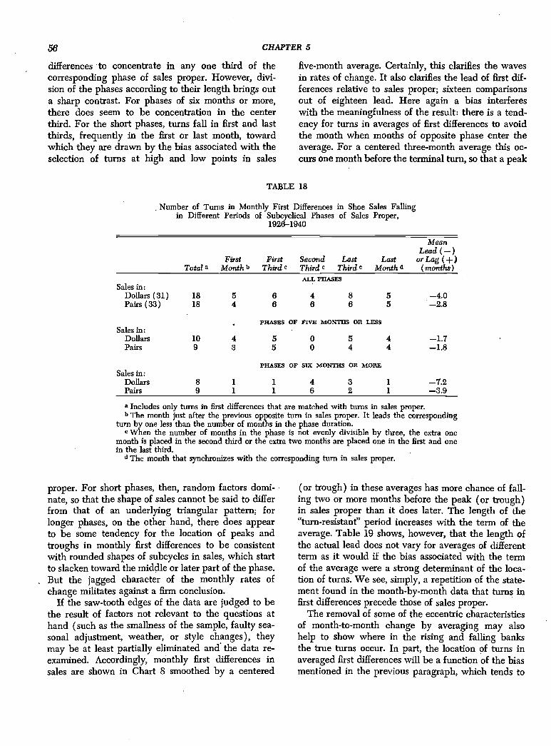
The most direct approach would seem to be to com-pute a first difference series (since it is rates of changethat we need to understand) and identify and studyits subcycical patterns. A five-month average was usedto help locate subcydical movements in the first differ-ences. It was not used in locating the month when the

55

fectly smooth, first differences would be a brokenhorizontal line above the axis during and be-low during recession. A random component added tosales would tend to place a peak in first differeAces withequal probability anywhere during the expansion phaseand a trough anywhere during a contraction phase.However, since turns were chosen at high and lowmonths in sales proper, there is a tendency for randomhighs and lows to occur at these times. The same tend-ency must then appear in rates of change. If, on the

Month-to-Month Differences in Doflar Shoe Sales, 1926—1941

Specific-subcycle peaks and troughs (broken and solid vertical lines) in dollar shoe sales (series in Appendix B)era used as reference frame.Specific-subcycle turns in first differences are marked by 0. When a specific turn is matched with a turn in thereference series, a horizontal line or vertical arrow indicates the association.The moving average of monthly first differences is centered.

turn The series is shown in Chart 8, whereits subcycles can be compared with those of salesproper by means of the vertical grid.

Patterns for first differences bear a definite arith-metic relation to those for sales. Consider first the tri-angular shape for sales. Were the course of sales per-

18 Turns are selected at the most extreme point except whenthere is reason to ignore it because of an immediately precedingor following extreme month of the opposite sign, or an alterna-tive month which, though not as extreme, is surrounded byother moderately extreme months of like sign. These proceduresare similar to those used in locating turns other than in firstdifference series.

other hand, sales moved in rounded waves of some sort,there would be a tendency for the peaks in first differ-ences to occur more frequently at one time during ex-pansion than at others—around the middle if the pat-tern were sine-like, or toward the end if retardationsimply preceded the fall—and the same would be trueof contractions.

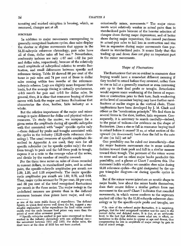
Table 18 supplies a crude test of the behavior of theactual data by dividing each specific-subcycle phase inshoe sales proper into three equal parts and noting inwhich third the turns in first differences occur. It in-dicates little tendency for peaks and troughs in first

1 -

CONSUMER PURCHASES

CHART 8

1926 1927 1928 1929 1930 1931 1932 1933 1934 1935 1936 1937 1938 1939 1940 1941

56 CHAPTER 5

differences to concentrate in any one third of thecorresponding phase of sales proper. However, divi-sion of the phases according to their length brings outa sharp contrast. For phases of six months or more,there does seem to be concentration in the centerthird. For the short phases, turns fall in first and lastthirds, frequently in the first or last month, towardwhich they are drawn by the bias associated with theselection of turns at high and low points in sales

five-month average. Certainly, this clarifies the wavesin rates of change. It also clarifies the lead of first dif-ferences relative to sales proper; sixteen comparisonsout of eighteen lead. Here again a bias interfereswith the meaningfulness of the result: there is a tend-ency for turns in averages of first differences to avoidthe month when months of opposite phase enter theaverage. For a centered three-month average this oc-curs one month before the terminal turn, so that a peak

TABLE 18

Number of Turns in Monthly First Differences in Shoe Sales Fallingin Different Periods of Subcyclical Phases of Sales Proper.

1926—1940

Mean

Total aFirst

Month bFirst

Third CSecond Last LastThird C Third C Month d

Lead (—)or Lag (+)

(months)ALL PHASES

Sales in:Dollars (31) 18 5 8 4 8 5 —4.0Pairs (33) 18 4 6 6 6 5 —2.8

PHASES OF FIVE MONTHS OR LESSSales in:

Dollars 10 4 5 0 5 4 —1.7Pairs 9 3 5 0 4 4 —1.8

PHASES OF SIX MONTHS OR MORESales in:

Dollars 8 1 1 4 3 1 —7.2Pairs 9 1 1 6 2 1 —3.9

a Includes only turns in first differences that are matched with turns in sales proper.b The month just after the previous opposite turn in sales proper. It leads the corresponding

turn by one less than the number of months in the phase duration.C When the number of months in the phase is not evenly divisible by three, the extra one

month is placed in the second third or the extra two months are placed one in the first and onein the last third.

d The month that synchronizes with the corresponding turn in sales proper.

proper. For short phases, then, random factors domi-nate, so that the shape of sales cannot be said to differfrom that of an underlying triangular pattern; forlonger phases, on the other hand, there does appearto be some tendency for the location of peaks andtroughs in monthly first differences to be consistentwith rounded shapes of subcycles in sales, which startto slacken toward the middle or later part of the phase.But the jagged character of the monthly rates ofchange militates against a firm conclusion.

If the saw-tooth edges of the data are judged to bethe result of factors not relevant to the questions athand (such as the smallness of the sample, faulty sea-sonal adjustment, weather, or style changes), theymay be at least partially eliminated the data re-examined. Accordingly, monthly first differences insales are shown in Chart 8 smoothed by a centered

(or trough) in these averages has more chance of fall-ing two or more months before the peak (or trough)in sales proper than it does later. The length of the"turn-resistant" period increases with the term of theaverage. Table 19 shows, however, that the length ofthe actual lead does not vary for averages of differentterm as it would if the bias associated with the termof the average were a strong determinant of the loca-tion of turns. We see, simply, a repetition of the state-ment found in the month-by-month data that turns infirst differences precede those of sales proper.

The removal of some of the eccentric characteristicsof month-to-month change by averaging may alsohelp to show where in the rising and falling banksthe true turns occur. In part, the location of turns inaveraged first differences will be a function of the biasmentioned in the previous paragraph, which tends to

CONSUMER PURCHASES 57

TABLE 19

Turns in Moving Averages of Monthly First Differences in PairShoe Sales Compared with Turns in Sales Proper, 1926—1940

MTerm of Average Matched Turns

(months) (number)

ean Lead (—)or Lag (+)(months)

ALL PHASES

Three 20 —8.3Five 20 —2.8Seven 18 —3.2

PHASES OF FIVE MONTHS OR LESS

Three 10 —2.2Five 10 —1.5Seven 9 —1.9

PHASES OF SIX MONTHS OR MORE

Three 10 —4.4Five 10 —4.0Seven 9 —4.6

Source: See series 33 in Appendix B for description of the pairshoe sales series. The moving averages are centered.

draw turns away from terminal and initial monthsof a phase in sales proper. There is a tendency, then,due to arithmetic rather than to the characteristicsof consumer buying to push turns, especially in fairlyshort phases, toward the center of the phase. To avoidthis bias we simply ignore the turn-resistant monthsin each phase and divide the rest into three parts asnearly equal in length as possible.1° If the pattern ofsales were triangular with a random component, theturns would occur with equal probability in any oneof the adjusted thirds (though there are faint biasestending to throw them in the first month of the firstthird and the last month of the last third, which maybe called "turn-prone" months) Unfortunately, since

I am indebted to Geoffrey Moore for suggesting this test.We plot change from the previous to current month at the samepoint as sales during the current month. For month-to-monthchange, then, the last observation of, say, expansion—the oneoccurring in the same month as the peak in sales proper—in-cludes no month of contraction. At the beginning of the expan-sion, this would be true of change plotted in the month just afterthe trough; relative to the following peak, this month wouldlead by one less than the number of months (L) in the phase.For a centered three-month moving average, the synchronousmonth at the end includes one month of recession, the lastmonth that does not resist turns is therefore the one before thepeak, —1; the first is L — 2. For centered five-month averages,the corresponding figures are —2 and L — 3. All months withshorter leads at the end or longer at the beginning of the phasewe call turn-resistant. Thus for, say, a three-month average ina nine-month phase, months with a timing of zero and —8 areignored. The remaining seven months are allotted to thirds asnearly equal in length as whole numbers permit.

20 The random factor previously mentioned—associated withthe selection of turns in sales proper at absolute high and lowpoints—would produce a lessened tendency here, for a highmonth to occur one month earlier at the end of the phase andone month later at the beginning than the last month in theaverage when a month of opposite phase entered. In addition,

this method loses many observations—the more thelonger the term of the average—only a centercd three-month average can be profitably used; comparisonscan be made for phases lasting five months or more,of which there are sixteen. Turns fall in the discardedturn-resistant months in three cases, in the first or lastthird in seven cases (all in the first and last—the turn-prone—months) and in the center third in five cases.For phases six months or longer, of which there areeight, turns fall in the first or last third in three cases(all in the turn-prone months) and in the center thirdin five cases. I conclude that when the device of amoving average is used to moderate the obscurity ofthe random component, the lead of firstseems to persist. Likewise it provides tender supportfor the presence of retardation toward the centralportions of at least the longer phases.

The National Bureau's standard nine-point patternsavoid some of the awkward characteristics of boththe monthly data and the moving averages, pro-vide summary descriptions of the shape of subcycles.Because of the brevity of many phases and the choppycharacter of the sales series, a good bit of thr poweras a smoothing device is lost when they are appliedto subcycles. Nevertheless, patterns for pair atid dollarshoe sales were computed in each of three ways; themeasuring rod with which to mark off suboycles inretail shoe sales and to locate each of the nine pointsfor each subcycle was taken first as the SLH-subcyclereference chronology, second as specific cycles in sales,third as specific cycles in a five-month moving averageof sales (the purpose here was to avoid the bias ofrandom highs at peaks, and lows at troughs). Thechange between the standing for Stages I and II, forII and III, etc., was calculated and ranked from oneto four for each expansion and each andthe rank standings averaged for each stage interval.Since the fastest rates for conforming movements wereranked one, a low average figure points to wherechange tended to be most rapid and a high one towhere it was slow. But as Table 20 shows, the figuresare not well differentiated. Significant differences ap-pear for expansion when stages are marked by the ref-erence chronology, and for contractions when they aremarked by the five-month moving average of shoe sales.In these four cases, the fastest rate of change occurs in

the month situated just to the inside of the initial and terminalturn-resistant months might be more likely than othcrs to beselected as a turn—the competition just before (at the beginningof phase) and just after (at the end of the phase) is bus severe.On two counts, then, there might be some tendency for turnsto occur in these months, which are the first and last months ofthe first and last thirds as described in the previous note.

21 See Appendix A, secs. 17 and 18. Phases of less than fourmonths were omitted.

58 CHAPTER 5

TABLE 20

Interstage Rates of Change in Nine-Point Patterns for Subcycles in Shoe Sales, 1926—1940 a

one of the central stages of the phase. But in the othercases—where results are presumably not statisticallysignificant—it occurs in a center stage twice and aninitial or terminal stage six times.

One further piece of evidence on the shape of sub-cycles in sales may be borrowed from the chapter thatfollows. There we find that the monthly pattern ofshoe buying is intimately associated with the monthlycourse of income payments to consumers. Shoe buyingand income have virtually all the same subcyclicalfluctuations and arrive at turns at nearly the same time.The average timing shows a lead of sales of 0.4 monthwith an average deviation of plus or minus 1.0 month.Because of the close relation, which can be inter-preted only as a causal impact of income on buying,it is pertinent to ask whether subcycles in the rateof change in income payments precede those of shoesales proper and also at what part of the phase in buy-ing retardation in income payments occurs. The rateof change in income payments is sufficiently smoothso that turns may be located with considerable assur-ance without recourse to moving averages; I inferthat the less easily visible retardations in buying wouldbe likely to occur at the same times. Turns in firstdifferences in consumer income are matched withthose in shoe sales proper at fourteen of the sixteenturns in dollar shoe sales that are marked between

1929 (when monthly data on income first becameavailable) and 1940. They lead in ten, synchronizein two, and lag in two cases; the average lead is 3.4months.22 Here, too, leads are longer, as indeed theyalmost must be, for longer than shorter phases, and thequestion occurs again whether they tend to occurtoward the center or at either end of each subcycical.phase. Dividing the phases in sales into thirds as.

nearly equal as possible, fourteen comparisons maybe made. First differences in income fall in the firstthird of sales in two cases, in the middle third in seven,and in the last third in three, and lag in two cases.For phases of six months or over, of which there weresix, the corresponding figures are none in the firstthird, four in the middle, and two in the last third.

I end with the baffled feeling of someone who tries.to examine the bottom of a shallow nool while wind

SIGNIFICANCEAVERAGE OF BANE POSITION FOR INTERSTACE RATES OF CHANCE TEST FOR

NUMBELIOFPHASES . Expansions Contractions RANKPOSITIONbExpan- Contrac- Stage Stage Stage Stage Stage Stage Stage Stage Expan- Contrac-

non tion Ito II II to 111 III to IV IV to V V to VI VI to VII VII to Viii VIII to 1X sion tionSHOESALES (1) (2) (3) (4) (5) (6) (7) (8) (9) (10) (11) (12)

STAGES MARKED BY SLH REFERENCE CHRONOLOGY

Dollars (31) 1]. 11 3.36 1.64 2.14 2.86 2.18 2.95 2.23 2.64 s. at 1% n.s.pairs (33) 11 11 3.27 1.55 2.09 3.09 2.00 2.82 2.36 2.82 s. at5% n.s.

STAGES MABXED BY SPECIFIC CYCLES IN SHOE SALES

Dollars 8 8 2.81 2.31 2.19 2.69 1.94 3.00 2.81 2.25 n.s. n.s.Pairs 10 10 2.05 2.40 3.25 2.30 2.05 2.50 2.75 2.70 n.s. n.s.

STAGES MARKED BY SPECIFIC CYCLES IN CENTERED FIVE-MONTH AVERAGE OF SHOE SALES

Dollars 7 8 2.50 2.29 2.71 2.50 3.38 1.88 1.88 2.88 n.s. s. at 5%Pairs 9 10 2.89 2.28 2.61 2.22 3.00 1.85 2.00 3.15 n.s. s. at 5%

In each section of the table, subcycles and the nine stages this process and of the nine-point patterns themselves, see Ap-of each subcycle in shoe sales are delineated in. the manner pendix A, secs. 17 and 18).indicated. For each subcycle, the standing at the initial trough b The rank position for the four interstage rates of change(Stage I), the peak (Stage V), and the terminal trough (Stage was considered not significant (n.s.) if it would be produced byIX) are centered three-month averages of sales. The rest of the chance more often than 5 out of 100 times (this is, of course, sig-expansion months are divided into three parts as nearly equal as nificance at the 5 per cent level). The Friedman test was usedpossible and the average for each part give standings for II, (see Milton Friedman, "A Comparison of Alternative Tests ofIII, and IV. Analogous calculations for contractions yield stand- Significance for the Problem of m Rankings," Annals of Matha-ings for VI, VII, and VIII. Change between each two successive matical Statistics, 1940, pp. 86—92).stages is averaged for all subcycles (for a further description of

22 Turns were matched after an allowance for a systematic.lead of one month in first differences in income payments, i.e.first differences in income payments were shifted back one month.before determining which turns could be related with those in.shoe sales proper. Rules were further relaxed in connection with.the long expansion from September 1934 to September 1937 inshoe sales, which was interrupted by a retardation in 1936. This.minor subcycle, which was not marked for first differences inincome payments with the bonus adjustment, was ignored inmatching turns. If it is not ignored, the average lead of first dif-ferences in income payments relative to sales is reduced to 2.5.months.

ruffles the water's surface. Contours suggestedand then erased. Investigation seems at least to createa strong probability that, could we transilluminate therandom component of the data, retardation wouldbe found to set in sometime before subcydical maximaor minima are reached. Further, there are traces inthe data that inflection points occur earlier in longerthan in shorter phases, indeed that they occur in thecentral sections of expansion or contraction; but evi-dence on this score provides no more than a startingpoint for inquiry.

The statistical evidence for retardations that pre-cede turns is supported by logical considerations. Ag-gregate shoe sales is an arithmetic construct—the sumof diverse experiences of thousands of retailers. At alltimes some of these retailers are experiencing a risein sales and a fall. When aggregate sales are ris-ing, more retailers are experiencing rises (or corn-pensatingly larger rises) than are experiencing falls.

59

A decline in the rate at which aggregate sales riseis occasioned by a decrease in the number of firmsexperiencing a rise, or a decrease in the size of theirrises (relative to the size of the declines), or a de-crease in both. An absolute fall in total sales takesplace when this situation passes the point where thenumber and size of falls exceed those of rise$. To saythat sales retard before they turn is simply anotherway of saying that the process of reversal takes time.This is not difficult to credit since most economicchange is gradual and cumulative. The same argumentapplies to the onset of revival.

On the other three questions investigated in thischapter—the trend, timing, and amplitude of fluctua-tion in consumer shoe buying—answers were clearand unequivocal. Because the language of both ques-tion and answer is primarily quantitative, I notrepeat here the findings summarized at the close ofeach of the three sections.

CONSUMER PURCHASES