Pattern Recognition Letters 33 (2012) 951–961

Contents lists available at SciVerse ScienceDirect

Pattern Recognition Letters

journal homepage: www.elsevier .com/locate /patrec

Prostate cancer grading: Gland segmentation and structural features q

Kien Nguyen a, Bikash Sabata b, Anil K. Jain a,⇑,1

a Michigan State University, East Lansing, MI 48824, USAb Ventana Medical Systems, Inc., 919 Hermosa Ct, Sunnyvale, CA 94085, USA

a r t i c l e i n f o

Article history:Available online 10 October 2011

Keywords:Prostate cancerBenignCarcinomaGleason grading systemGland segmentationNuclei

0167-8655/$ - see front matter � 2011 Elsevier B.V. Adoi:10.1016/j.patrec.2011.10.001

q A preliminary version of this paper appeared inICPR, Istanbul, August 2010.⇑ Corresponding author. Tel.: +1 517 355 9282.

E-mail addresses: nguye231@msu.edu (K. Nguyencom (B. Sabata), jain@cse.msu.edu (A.K. Jain).

1 Also affiliated to Department of Brain & CognitiveSeoul.

a b s t r a c t

In this paper, we introduce a novel approach to grade prostate malignancy using digitized histopatholo-gical specimens of the prostate tissue. Most of the approaches proposed in the literature to address thisproblem utilize various textural features computed from the prostate tissue image. Our approach differsin that we only focus on the tissue structure and the well-known Gleason grading system specification.The color space representing the tissue image is investigated and basic components of the prostate tissueare detected. The components and their structural relationship constitute a complete gland region. Tissuestructural features extracted from gland morphology are used to classify a tissue pattern into three majorcategories: benign, grade 3 carcinoma and grade 4 carcinoma. Our experiments show that the proposedmethod outperforms a texture-based method in the three-class classification problem and most of thetwo-class classification problems except for the grade 3 vs grade 4 classification. Based on these results,we propose a hierarchical (binary) classification scheme which utilizes the two methods and obtains85.6% accuracy in classifying an input tissue pattern into one of the three classes.

� 2011 Elsevier B.V. All rights reserved.

1. Introduction grading (Gleason, 1977, 1992), which assigns a numerical grade

Prostate cancer is a type of cancer that occurs in men’s repro-ductive system. In the United States, it is the second most preva-lent cancer in men and it is also one of the leading causes ofdeath by cancer (in 2006, prostate cancer developed in 203,415men and killed 28,372 men) (US Cancer Statistics Working Group,2010). Prostate cancer grows slowly with very few symptoms; itdevelops mostly in men over the age of fifty. Prostate cancer is con-sidered serious because of the threat of its invasion (metastasis)into other organs such as bones, bladder and rectum. The prognosisinvolves a screening (such as digital rectal examination or pros-tate-specific antigen (PSA) test (Catalona et al., 1991)) and, ifnecessary, a follow-up prostate biopsy. After an unsuspected can-cer is revealed via the screening, a biopsy is used to confirm it. ACT scan or a bone scan can be employed additionally to determinethe spread of the cancer.

The biopsy is conducted by a radiologist or a urologist. First, aprostate tissue sample is removed from the patient for inspectionunder a microscope. A grade is then reported for the tumor derivedfrom the tissue. The most widely used grading method is Gleason

ll rights reserved.

the Proceedings of the 20th

), bikash.sabata@bioimagene.

Engineering, Korea University,

from 2 to 10 to the tumor. The grade is based solely on structuralfeatures of the tissue and excludes cytological features(Mason, 1964). In this grading method, a pathologist finds the mostpredominant and the second most predominant histologicalcarcinoma patterns in the tissue, assigns each of them a score(from 1 to 5) and adds the two scores together to obtain the finalGleason grade (2 to 10) for the tissue. The grade of each carcinomapattern is based on its differentiation (how much of its structureresembles a normal pattern structure). A grade 1 carcinoma pat-tern is very well differentiated and a grade 5 carcinoma patternis very poorly differentiated. The change in tissue structure is goodevidence for this differentiation. More specifically, in Gleasongrades 1 and 2, most of the glands appear as single units, separatedfrom each other, densely packed, and there is no infiltration ofthese glands into benign tissue areas (this is very close to the struc-ture of a normal tissue). Gleason Grade 3, the most common case ofcarcinoma, is characterized by the invasion of small glands into themuscle (stroma). In Gleason grade 4, glands are fused with eachother and poorly defined; glands are not well-separated by stromaas in lower grades. Finally, in Gleason grade 5, there is no evidenceof the formation of gland units in the pattern. A visual summariza-tion of these five grades can be found in Fig. 1. Pathologists face anumber of difficulties in manually diagnosing prostate cancer, i.e.to look at the prostate tissue under a microscope is tedious andtime-consuming. Moreover, the diagnostic accuracy depends onthe personal skill and experience of a pathologist. These problemsmotivate the research and development for automating thediagnosis and prognosis processes.

Fig. 1. Five grades of the Gleason grading applied to histological patterns of the prostate tissue.

952 K. Nguyen et al. / Pattern Recognition Letters 33 (2012) 951–961

In most digital pathology studies on computer-aided prognosisfor prostate cancer, textural features of the image and structuralfeatures of the tissue have been widely used. Diamond et al.(2004) used co-occurrence texture features (Haralick et al., 1973)to classify each 100 � 100 sub-region in a tissue image into eitherstroma or prostatic carcinoma. In addition, lumen area was usedto discriminate benign tissue from the other two classes. They re-ported 79.3% accuracy when evaluating the algorithm on sub-re-gions of 8 tissue images (40� magnification). A cancer vs non-cancer classification problem which used 594 features includingfirst-order statistics (average, median, standard deviation), co-occurrence and wavelet features was addressed in Doyle et al.(2006). The algorithm was implemented at three different scalesof the image. At each scale, a Bayes classifier was designed for eachfeature individually, resulting in 594 base learners for AdaBoost.The reported accuracy was 88% on a dataset of 22 images (40�mag-nification). In Tai et al. (2010), fractal dimension features were cal-culated for the tissue image and the low frequency sub-bands of theimage to discriminate the textural discrepancy between low gradeand high grade carcinoma. By using an SVM classifier with leave-one-out technique, the method achieved 86.3% accuracy for theclassification of 1,000 prostatic biopsy images into normal, grade3, grade 4 and grade 5 classes. A multiwavelet transform was usedas the main texture analysis tool in Khouzani and Zadeh (2003). Thefeatures used for classification included entropy and energy derivedfrom the multiwavelet coefficients of the image. Ten different typesof multiwavelet were evaluated on a dataset of 100 prostate sampleimages (100�magnification) of grades 2, 3, 4 and 5, resulting in thebest accuracy of 97%. In another study, Tabesh et al. (2007) em-ployed both global features of the entire image and local featuresof every object in the image. Global features included color histo-gram, fractal features, texture and morphometry of the image. Localfeatures were computed for histological objects such as nuclei, stro-ma and lumen, which were extracted by the MAGIC system (Teve-rovskiy et al., 2004). They achieved 96.7% accuracy for tumor-nontumor classification (fivefold cross validation with 367 images)and 81% accuracy for low grade-high grade classification (fivefoldcross validation with 268 images). All images were at 20�magnifi-cation. A segmentation-based method was presented in Naik et al.

(2008). They first used a Bayesian classifier to place every pixel inthe image into one of the three classes: lumen, nuclei and cyto-plasm based on its color. Lumen pixels were first grouped togetherand lumen objects were then identified as the groups satisfying thegland size constraint. The inner boundary of the glands, which is theborder of the nuclei and the cytoplasm surrounding the lumen, wasdetected using a level set formulation. Eight shape features for eachof the lumen and the gland inner boundary were calculated. A tis-sue was classified into benign, a grade 3 carcinoma or a grade 4 car-cinoma via an SVM classifier. However, by using a dataset thatincluded 44 images at 40� magnification, they only reported re-sults of two-class classifications: 86.35% accuracy when classifyinggrade 3 carcinoma and benign, 92.9% accuracy when classifyinggrade 4 carcinoma and benign, and 95.19% accuracy when classify-ing grade 3 carcinoma and grade 4 carcinoma. Three-class classifi-cation result was not reported. Table 1 summarizes the relatedstudies discussed in this section.

In this study, we present a segmentation-based method to clas-sify a tissue pattern into three common cases based on Gleasongrading: benign, grade 3 and grade 4 carcinoma. However, unlikeNaik et al. (2008), we incorporate nucleus and blue mucin informa-tion into the glandular structures which are used for the classifica-tion. It is apparent from the tissue pattern image that nucleusdistribution changes remarkably among various cancer stages (inbenign tissue, nuclei form a ring on the gland boundary and scatterin other areas (Fig. 8(a)) while in grade 4 carcinoma, nuclei distrib-ute more uniformly over the glandular regions (Fig. 8(c))) and mu-cin appears commonly in cancerous glands (Fig. 8(b)). While agland region in Naik et al. (2008) solely consists of lumen andinternal cytoplasm region, our segmentation procedure leads tocomplete glands which include their nucleus boundaries. More-over, the structural features extracted in our method do not requirea very high magnification (like 40� in Naik et al., 2008) to achievestate of the art classification results. The proposed algorithm is de-signed to work for images created from the Hematoxylin and Eosin(H&E) staining method (Kiernan, 2001). The outline of the method-ology is delineated in the flowchart of Fig. 2. Given an input tissuepattern, we first segment glands from the stroma area (thiscomprises steps 1, 2, 3, 4 in the flowchart). Once gland regions

Table 1Summary of major classification studies on prostate cancer.

Authors Features used Dataset size (magnification) Classes Accuracy

Diamond et al.(2004)

Co-occurrence texture features and lumen area 100 � 100 sub-regions of 8 tissueimages (40� magnification)

Stroma, benign tissuea andprostatic carcinomaa

79.3%

Doyle et al. (2006) First-order statistics (average, median, standard deviation),co-occurrence and wavelet features

22 images (40� magnification) Cancera vs noncancera 88%

Tai et al. (2010) Fractal dimension features 1000 images Normala, grade 3, grade 4 andgrade 5

86.3%

Khouzani andZadeh (2003)

Entropy and energy of the multiwavelet coefficients 100 images (100� magnification) Grades 2, 3, 4 and 5carcinoma

97%

Tabesh et al.(2007)

Global features of the image and local features ofhistological objects

268 images (20� magnification) Low grade vs high grade 81%

367 images (20 �magnification) Tumora vs non-tumora 96.7%Naik et al. (2008) Shape features of the lumen and the gland inner boundary 44 images (40 �magnification) Grade 3 vs benign 86.35%

Grade 4 vs benign 92.9%Grade 3 vs grade 4 95.19%

Proposedhierarchicalscheme

Glandular structural features and co-occurrence texturefeatures

82 ROIs (10� magnification) Benign, grade 3 and grade 4carcinoma

85.6%

a Different terminologies which have the same meaning were used in the related work. Cancer, tumor and carcinoma refer to the tissues which are detected to havemalignant properties of a cancer (cells grow aggressively, invade the surrounding tissues and spread to the non-adjacent tissues). Noncancer, normal, benign and nontumorrefer to the tissues which do not have the properties of cancer.

Fig. 2. Methodology outline.

Fig. 3. A gland segmentation result obtained by a level set method in Naik et al.(2008). The blue and black curves show the segmented gland which only includeslumen and cytoplasm regions. The yellow lines delineate the gaps between thenuclei layers. (For interpretation of the references to colour in this figure legend, thereader is referred to the web version of this article.)

K. Nguyen et al. / Pattern Recognition Letters 33 (2012) 951–961 953

are identified, we extract fifteen features from the pattern based onglandular structures (step 5 of the flowchart). Finally, these fea-tures become inputs to different classifiers to determine the carci-noma grade of the input pattern (step 6 in the flowchart).

The rest of the paper is organized as follows. Section 2 describesthe gland segmentation algorithm, Section 3 explains the featuresextracted from the gland regions, Section 4 presents experimentalresults using different classifiers and Section 5 concludes thepaper.

2. Segmentation of gland units

In a normal prostate tissue (Fig. 4(a)), stroma (pink2 regions)serves as background and gland units are foreground objects. A glandunit does not have any fixed shape or size; it can be oval, round orbranchy and it can be either small or very large. Hence, we cannotutilize Active Shape Model (Cootes et al., 1995) or Active Appearance

2 For interpretation of color in Figs. 4 and 8, the reader is referred to the webversion of this article.

Model (Cootes et al., 2001) to detect gland objects. In Naik et al.(2008), the authors used a level set approach to segment glands inthe tissue. However, the gland segments obtained in their approachonly include lumen and cytoplasm regions (Fig. 3) while we want tocapture the entire gland area which also includes nuclei on the glandboundary. Since there are usually multiple layers of nuclei on thegland boundary and there are gaps between these layers (the yellowlines in Fig. 3 delineate these gaps), it is difficult to force the level setcurve to capture all of the nuclei on the gland boundary. In a stan-dard energy minimization formulation of the level set, the curve isattracted toward high gradient magnitude regions (Li et al., 2005).These high gradient magnitude regions can be the edges of the nucleior can be the nuclei likelihood image as defined in Naik et al. (2008).Since the gaps between nuclei layers must have low gradient magni-tude, it is difficult for a level set curve to pass these gaps and em-brace all the nuclei.

Consequently, we rely on the structure of glands to segmentthem from the tissue background. Each gland unit has a boundaryof epithelial cells which include epithelial nuclei (blue dots) mixedwith epithelial cytoplasm (purple) and lumina (white) in the cen-ter. In some cancer tissues, blue mucin may be found to invadethe lumina (Fig. 8(b)). In short, nuclei, cytoplasm, stroma, lumenand mucin are five basic components which appear in different col-ors in a prostate tissue image stained by the H&E method. As a

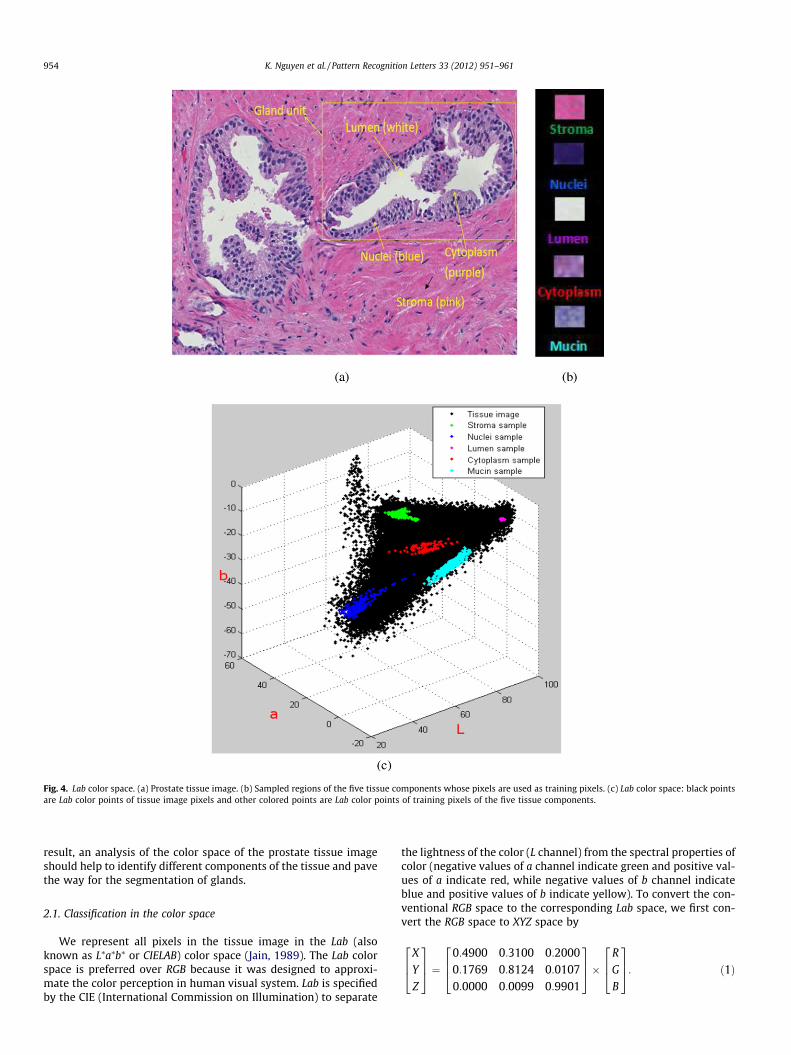
Fig. 4. Lab color space. (a) Prostate tissue image. (b) Sampled regions of the five tissue components whose pixels are used as training pixels. (c) Lab color space: black pointsare Lab color points of tissue image pixels and other colored points are Lab color points of training pixels of the five tissue components.

954 K. Nguyen et al. / Pattern Recognition Letters 33 (2012) 951–961

result, an analysis of the color space of the prostate tissue imageshould help to identify different components of the tissue and pavethe way for the segmentation of glands.

2.1. Classification in the color space

We represent all pixels in the tissue image in the Lab (alsoknown as L⁄a⁄b⁄ or CIELAB) color space (Jain, 1989). The Lab colorspace is preferred over RGB because it was designed to approxi-mate the color perception in human visual system. Lab is specifiedby the CIE (International Commission on Illumination) to separate

the lightness of the color (L channel) from the spectral properties ofcolor (negative values of a channel indicate green and positive val-ues of a indicate red, while negative values of b channel indicateblue and positive values of b indicate yellow). To convert the con-ventional RGB space to the corresponding Lab space, we first con-vert the RGB space to XYZ space by

X

Y

Z

264

375 ¼

0:4900 0:3100 0:20000:1769 0:8124 0:01070:0000 0:0099 0:9901

264

375�

R

G

B

264

375: ð1Þ

K. Nguyen et al. / Pattern Recognition Letters 33 (2012) 951–961 955

The elements of the transformation matrix were derived in Fairmanet al. (1997). Next, the XYZ space is converted to Lab space by

L ¼ 116f ðY=YnÞ � 16 ð2Þa ¼ 500½f ðX=XnÞ � f ðY=YnÞ� ð3Þb ¼ 200½f ðY=YnÞ � f ðZ=ZnÞ� ð4Þ

where

f ðtÞ ¼t1=3 if t > 6

29

� �3

13

296

� �2t þ 4

29 otherwise;

(ð5Þ

and Xn, Yn, Zn are the white point tristimulus values in XYZ (Wikipe-dia contributors, 2010). Each pixel p in the image domain is mappedto a point c(p) in the Lab space, where c(p) is the three-dimensional(L,a,b) color vector of pixel p. Notice that this is a many-to-onemapping because several pixels can have the same (L,a,b) color vec-tor. In Fig. 4(c), we demonstrate the Lab color space of the image inFig. 4(a). Our goal is to determine to which component of the tissueeach image pixel p belongs. Based on the fact that the number ofpoints in the Lab space is smaller than the number of pixels in theimage, we can (i) classify points in the Lab color space into five clas-ses (representing the five components) and (ii) use the classificationresults to assign each image pixel a label of the corresponding com-ponent. This can be done due to the known mapping between pixelsin the image and points in the Lab space. To facilitate the classifica-tion, we sample pixels in local regions (approximately 18 � 22 pix-els) for each component (Fig. 4(b)) from a training tissue image. LetCi denote the class corresponding to the ith tissue component (werefer to stroma, nuclei, cytoplasm, lumen, mucin as the 1st, 2nd,

3rd, 4th and 5th components, respectively) and Di ¼ xij

n oni

j¼1denote

the set of ni training pixels of class Ci. The Lab color points of thesetraining pixels (we call training points for short), denoted by

cðDiÞ ¼ c xij

� �n oni

j¼1

� �5

i¼1, are shown in color in Fig. 4(c) while the

Lab color points of the tissue image pixels are shown in black inthe same figure.

The training points create a Voronoi tessellation (Franz, 1991) of

the Lab space (each training point c xij

� �is associated with one con-

vex polygon which includes all points closer to it than any othertraining point). Each unclassified point c(p) (black points inFig. 4(c)) is assigned to the same class associated with the training

Fig. 5. Classification in the Lab space (a) and tissue pixel labeling (b). The same color isimage; cytoplasm, nuclei, lumen, stroma and blue mucin are denoted by green, blue, pinkare invisible because they are occluded by points of other classes and (ii) multiple pixels ithe references to colour in this figure legend, the reader is referred to the web version o

point of the polygon to which it belongs. Once the points in theLab space are classified (Fig. 5(a)), each pixel in the tissue image isassigned one of the five labels in L = {LS,LN,LC,LL,LM} correspondingto the five components (stroma, nuclei, cytoplasm, lumen, mucin)(Fig. 5(b)) via the mapping of points in the Lab color space and pixelsin the image. Formally, a pixel p is assigned a label Li 2 L, l(p) = Li such

that lðpÞ ¼ arg minLiminj2½1;ni �

dðcðpÞ; c xij

� �Þ

� , where d cðpÞ; c xi

j

� �� �is

the Euclidean distance between c(p) and c xij

� �in the Lab space.

2.2. Identify glandular components

Once all the pixels have been classified, we identify nuclei andlumina, the two most important components of the gland. A binaryimage indicating nucleus pixels is derived from pixel labels(Fig. 6(a)) and a connected component algorithm is applied to thisbinary image to form the nucleus objects. The four-connectivityproperty, which only considers the top, left, bottom, and rightneighbors of each pixel, is employed. Lumen objects (commonly lo-cated in the center of glands) are also created in the same manner(Fig. 7(a)). Nucleus objects and lumen objects are sequentially uti-lized in the following two procedures.

2.3. Construct gland boundary

In the anatomical structure of a prostate tissue, epithelial celllayers comprising nuclei and cytoplasm constitute the glandboundary. Moreover, as we can see in Fig. 4(a) both nuclei andcytoplasm gather densely around the gland but scatter sparselyin other areas (for example, stroma). This motivates us to developa two-step algorithm for constructing gland boundary.

In the first step, nucleus objects (obtained from Section 2.2) areenlarged by combining them with cytoplasm pixels. An enlargedinstance N0i of a nucleus object Ni is defined as: N0i ¼ fpjp 2 Ni or(l(p) = LC and kp,centroid(Ni)k2 6 dn)}, where p is a pixel in the im-age, LC is the label of the cytoplasm pixel (defined in the previouspart) and parameter dn is empirically estimated by half the averagedistance between neighboring nuclei in the gland boundary andcentroid(Ni) is the centroid of the object Ni. The goal of this stepis to facilitate the grouping of neighboring nuclei in the secondstep.

used for a classified point in the Lab space and the associated labeled pixel in the, red, cyan, respectively in both (a) and (b). Note that (i) several points of each class

n the image can be mapped to one point in the Lab color space. (For interpretation off this article.)

Fig. 6. Gland boundary segments are generated from nucleus objects.

956 K. Nguyen et al. / Pattern Recognition Letters 33 (2012) 951–961

In the second step, we group enlarged nuclei which intersecteach other to construct gland boundary segments. Each segmentmay contain only one isolated enlarged nucleus or several enlargednuclei, depending on the nucleus density in the area. More con-cretely, a gland boundary segment GB can be (i) a single enlargednucleus N0i if 8N0j – N0i; N0i \ N0j ¼ ; or (ii) a group of enlarged nucleiN0k; . . . ;N0kþm

� �, where 8N0i ðk 6 i 6 kþmÞ; 9N0j ðk 6 j 6 kþmÞ such

that i – j and N0i \ N0j –;.As nuclei are not uniformly dense everywhere on the boundary,

we may not obtain a complete boundary segment for each gland.Thus, this stage can generate multiple segments for each glandboundary. Fig. 6(b) demonstrates the output of gland boundary

Fig. 7. Expansion procedure of the lumen to unify glan

construction applied to the image of Fig. 4(a). The next procedurecombines these segments into the final gland regions.

2.4. Segment complete gland units

Again, we rely on the glandular structure (lumina lie in the cen-ter of glands and are embraced by gland boundary) to implementan algorithm for unifying lumen objects (obtained from Section 2.2)with gland boundary segments (obtained from Section 2.3) to formcomplete gland units. The non-tissue areas (which appear whitenear the image boundary, e.g. in Fig. 8(a) and (c)) are discriminatedfrom lumen objects by their contacts with the image boundary. The

dular components and form complete gland units.

K. Nguyen et al. / Pattern Recognition Letters 33 (2012) 951–961 957

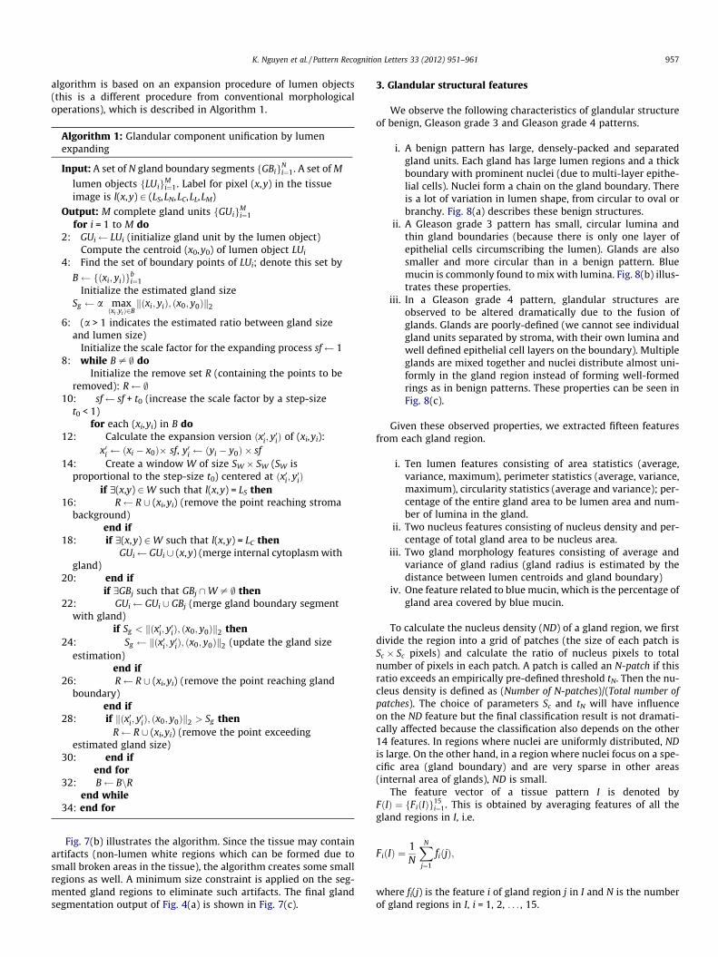
algorithm is based on an expansion procedure of lumen objects(this is a different procedure from conventional morphologicaloperations), which is described in Algorithm 1.

Algorithm 1: Glandular component unification by lumenexpanding

Input: A set of N gland boundary segments fGBigNi¼1. A set of M

lumen objects fLUigMi¼1. Label for pixel (x,y) in the tissue

image is l(x,y) 2 (LS,LN,LC,LL,LM)

Output: M complete gland units fGUigMi¼1

for i = 1 to M do2: GUi LUi (initialize gland unit by the lumen object)

Compute the centroid (x0,y0) of lumen object LUi

4: Find the set of boundary points of LUi; denote this set by

B fðxi; yiÞgbi¼1

Initialize the estimated gland sizeSg a max

ðxi ;yiÞ2Bkðxi; yiÞ; ðx0; y0Þk2

6: (a > 1 indicates the estimated ratio between gland sizeand lumen size)

Initialize the scale factor for the expanding process sf 18: while B – ; do

Initialize the remove set R (containing the points to beremoved): R ;

10: sf sf + t0 (increase the scale factor by a step-sizet0 < 1)

for each (xi,yi) in B do12: Calculate the expansion version ðx0i; y0iÞ of (xi,yi):

x0i ðxi � x0Þ� sf, y0i ðyi � y0Þ � sf14: Create a window W of size SW � SW (SW is

proportional to the step-size t0) centered at ðx0i; y0iÞif $(x,y) 2W such that l(x,y) = LS then

16: R R [ (xi,yi) (remove the point reaching stromabackground)

end if18: if $(x,y) 2W such that l(x,y) = LC then

GUi GUi [ (x,y) (merge internal cytoplasm withgland)

20: end ifif $GBj such that GBj \W – ; then

22: GUi GUi [ GBj (merge gland boundary segmentwith gland)

if Sg < kðx0i; y0iÞ; ðx0; y0Þk2 then24: Sg kðx0i; y0iÞ; ðx0; y0Þk2 (update the gland size

estimation)end if

26: R R [ (xi,yi) (remove the point reaching glandboundary)

end if28: if kðx0i; y0iÞ; ðx0; y0Þk2 > Sg then

R R [ (xi,yi) (remove the point exceedingestimated gland size)

30: end ifend for

32: B BnRend while

34: end for

Fig. 7(b) illustrates the algorithm. Since the tissue may contain

artifacts (non-lumen white regions which can be formed due tosmall broken areas in the tissue), the algorithm creates some smallregions as well. A minimum size constraint is applied on the seg-mented gland regions to eliminate such artifacts. The final glandsegmentation output of Fig. 4(a) is shown in Fig. 7(c).

3. Glandular structural features

We observe the following characteristics of glandular structureof benign, Gleason grade 3 and Gleason grade 4 patterns.

i. A benign pattern has large, densely-packed and separatedgland units. Each gland has large lumen regions and a thickboundary with prominent nuclei (due to multi-layer epithe-lial cells). Nuclei form a chain on the gland boundary. Thereis a lot of variation in lumen shape, from circular to oval orbranchy. Fig. 8(a) describes these benign structures.

ii. A Gleason grade 3 pattern has small, circular lumina andthin gland boundaries (because there is only one layer ofepithelial cells circumscribing the lumen). Glands are alsosmaller and more circular than in a benign pattern. Bluemucin is commonly found to mix with lumina. Fig. 8(b) illus-trates these properties.

iii. In a Gleason grade 4 pattern, glandular structures areobserved to be altered dramatically due to the fusion ofglands. Glands are poorly-defined (we cannot see individualgland units separated by stroma, with their own lumina andwell defined epithelial cell layers on the boundary). Multipleglands are mixed together and nuclei distribute almost uni-formly in the gland region instead of forming well-formedrings as in benign patterns. These properties can be seen inFig. 8(c).

Given these observed properties, we extracted fifteen featuresfrom each gland region.

i. Ten lumen features consisting of area statistics (average,variance, maximum), perimeter statistics (average, variance,maximum), circularity statistics (average and variance); per-centage of the entire gland area to be lumen area and num-ber of lumina in the gland.

ii. Two nucleus features consisting of nucleus density and per-centage of total gland area to be nucleus area.

iii. Two gland morphology features consisting of average andvariance of gland radius (gland radius is estimated by thedistance between lumen centroids and gland boundary)

iv. One feature related to blue mucin, which is the percentage ofgland area covered by blue mucin.

To calculate the nucleus density (ND) of a gland region, we firstdivide the region into a grid of patches (the size of each patch isSc � Sc pixels) and calculate the ratio of nucleus pixels to totalnumber of pixels in each patch. A patch is called an N-patch if thisratio exceeds an empirically pre-defined threshold tN. Then the nu-cleus density is defined as (Number of N-patches)/(Total number ofpatches). The choice of parameters Sc and tN will have influenceon the ND feature but the final classification result is not dramati-cally affected because the classification also depends on the other14 features. In regions where nuclei are uniformly distributed, NDis large. On the other hand, in a region where nuclei focus on a spe-cific area (gland boundary) and are very sparse in other areas(internal area of glands), ND is small.

The feature vector of a tissue pattern I is denoted byFðIÞ ¼ fFiðIÞg15

i¼1. This is obtained by averaging features of all thegland regions in I, i.e.

FiðIÞ ¼1N

XN

j¼1

fiðjÞ;

where fi(j) is the feature i of gland region j in I and N is the numberof gland regions in I, i = 1, 2, . . . , 15.

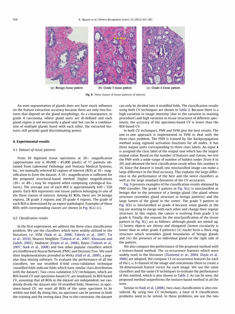
Fig. 8. Three classes of tissue patterns of interest.

958 K. Nguyen et al. / Pattern Recognition Letters 33 (2012) 951–961

An over-segmentation of glands does not have much influenceon the feature extraction accuracy because there are only two fea-tures that depend on the gland morphology. As a consequence, ingrade 4 carcinoma, where gland units are ill-defined and eachgland region is not necessarily a gland unit but can be a combina-tion of multiple glands fused with each other, the extracted fea-tures still provide good discriminating power.

4. Experimental results

4.1. Dataset of tissue patterns

From 26 digitized tissue specimens at 20� magnification(approximate size is 90,000 � 45,000 pixels) of 17 patients ob-tained from Lakewood Pathology and Ventana Medical Systems,Inc., we manually selected 82 regions of interest (ROI) at 10�mag-nification to form the dataset. A 10� magnification is sufficient forthe proposed structural-based method (higher magnifications(20� or 40�) may be required when computing cytological fea-tures). The average size of each ROI is approximately 620 � 550pixels. Each ROI represents one tissue pattern belonging to one ofthe three classes of interest. Among 82 ROIs, there are 34 benignregions, 28 grade 3 regions and 20 grade 4 regions. The grade ofeach ROI is determined by an expert pathologist. Examples of theseROIs with corresponding classes are shown in Fig. 8(a)–(c).

4.2. Classification results

In the first experiment, we address the three-class classificationproblem. We use the classifiers which were widely utilized in theliterature, i.e. SVM (Naik et al., 2008; Tabesh et al., 2007; Taiet al., 2010), Nearest Neighbor (Tabesh et al., 2007; Khouzani andZadeh, 2003), Adaboost (Doyle et al., 2006), Bayes (Tabesh et al.,2007; Naik et al., 2008) and two other popular classifiers whichare feedforward Neural Network (FNN) and Decision Tree. We usedtheir implementations provided in Weka (Hall et al., 2009), a pop-ular data mining software. To evaluate the performance of all theclassifiers, we use stratified K-fold cross-validation technique(stratified folds indicate folds which have similar class distributionwith the dataset). Two cross-validation (CV) techniques, which areROI-based CV and specimen-based CV, are employed. In ROI-basedCV, assuming that all ROIs in the dataset are independent, we ran-domly divide the dataset into 10 stratified folds. However, in spec-imen-based CV, we want all ROIs of the same specimen to liewithin one fold. By doing this, no specimen can be present in boththe training and the testing data. Due to the constraint, the dataset

can only be divided into 4 stratified folds. The classification resultsusing both CV techniques are shown in Table 2. Because there is ahigh variation in image intensity (due to the variation in stainingprocedure) and high variation in tissue structures of different spec-imens, the accuracy of the specimen-based CV is lower than theROI-based CV.

In both CV techniques, FNN and SVM give the best results. Theone-vs-one approach is implemented in SVM to deal with thethree-class problem. The FNN is trained by the backpropagationmethod using sigmoid activation functions for all nodes. It hasthree output units corresponding to three class labels. An input xis assigned the class label of the output unit which has the largestoutput value. Based on the number of features and classes, we testthe FNN with a wide-range of number of hidden nodes (from 8 to20) and obtained the best classification result when this number is16. Since the dataset is small, one misclassified image can make alarge difference in the final accuracy. This explains the large differ-ence in the performance of the best and the worst classifiers aswell as the large standard deviation of the CV accuracies.

Fig. 9 presents examples of the classification results obtained byFNN classifier. The grade 3 pattern in Fig. 9(a) is misclassified asbenign due to the presence of a benign gland (the gland whosestructure resembles gland structure in benign patterns) and thelarge lumen of the gland in the center. The grade 3 pattern inFig. 9(b) is misclassified as grade 4 because some glands at thetop are starting to merge with each other and change their regularstructure. In this region, the cancer is evolving from grade 3 tograde 4. Finally, the reasons for the misclassification of the tissuepattern in Fig. 9(c) are as follows: although glands are mixed up,(i) lumen objects are skinny and elongated (lumen circularity islower than in other grade 4 patterns) (ii) nuclei form a thick ringstructure which resembles gland boundaries of benign glandsand (iii) the presence of an individual gland on the right side ofthe pattern.

We also compare the performance of the proposed method witha texture-based method. The co-occurrence features which werewidely used in the literature (Diamond et al., 2004; Doyle et al.,2006) are adopted. We compute 13 co-occurrence features for eachof the L, a, b channel of the image and concatenate them to create a39-dimensional feature vector for each image. We use the sameclassifiers and the same CV techniques to evaluate the performanceof this method, which is also shown in Table 2. As can be seen, theproposed method outperforms the texture-based method in all thetests.

Similar to Naik et al. (2008), two-class classification is also con-sidered. By using two CV techniques, a total of 8 classificationproblems need to be solved. In these problems, we use the two

Table 2Accuracy (%) and standard deviation of three-class classification for the proposedmethod and texture-based method evaluated by ROI-based CV and specimen-basedCV. Bold values are the best accuracies in each column.

Classifier ROI-based CV Specimen-based CV

Proposedmethod

Texture-basedmethod

Proposedmethod

Texture-basedmethod

Adaboost (with decisionstump as weakclassifier)

75.3(12.7)

56.1 (10.9) 68.3(06.7)

52.2 (04.3)

Nearest Neighbor 80.3(14.0)

72.9 (13.7) 69.5(11.4)

57.5 (19.5)

Decision Tree (C4.5) 79.0(11.2)

72.1 (16.3) 68.4(11.4)

62.4 (18.9)

Naive Bayes 81.5(08.6)

70.4 (18.1) 71.9(09.3)

59.9 (21.7)

SVM (squaredexponential kernel)

87.8(09.6)

81.7 (10.9) 75.1(10.6)

69.9 (15.7)

Feedforward NeuralNetwork with onehidden layer

87.8(13.7)

83.0 (13.8) 74.5(07.8)

71.4 (15.5)

Table 3Best accuracies achieved for 8 different two-class classification problems of the twomethods (proposed and texture-based) evaluated by two cross-validation (CV)techniques. For the proposed method, SVM is better than FNN for all the 8 problems.For the texture-based method, the best classifier and its accuracy are shown for eachproblem. Bold values indicate the method with higher accuracy for each classificationproblem.

Classificationproblem

ROI-based CV Specimen-based CV

Proposedmethod

Texture-basedmethod

Proposedmethod

Texture-basedmethod

Benign vsgrade 3

98.3 (05.0) 86.9 (14.5)(by FNN)

93.2 (05.5) 74.9 (08.3)(by FNN)

Benign vsgrade 4

96.0 (12.0) 93.0 (11.4)(by SVM)

89.5 (15.0) 87.8 (13.7)(by FNN)

Grade 3 vsgrade 4

85.5 (13.1) 86.0 (12.8)(by SVM)

70.7 (22.5) 84.4 (12.3)(by SVM)

Benign vscarcinoma

97.5 (05.0) 86.5 (12.8)(by SVM)

94.2 (07.4) 80.3 (08.3)(by FNN)

K. Nguyen et al. / Pattern Recognition Letters 33 (2012) 951–961 959

classifiers which performed the best in the three-class problem(SVM and FNN). We also compare the proposed method and thetexture-based method on these problems. For the proposed meth-od, SVM gives better results than FNN in all two-class classification

Fig. 9. Examples of classification results. Misclassifications: (a) Grade 3 pattern misclassmisclassified as benign; Correct classifications: (d) Benign pattern, (e) grade 3 pattern a

problems. The accuracy of FNN is approximately 4% lower thanSVM, on average. However, in the texture-based method, SVM out-performs FNN in some classification problems and FNN outper-forms SVM in other problems. The best classification results ofthe two methods in 8 different classification problems are reportedin Table 3. As can be seen, the proposed method is better than thetexture-based method in all problems except for the grade 3 vsgrade 4 classification problem. Since the dataset contains several

ified as benign, (b) Grade 3 pattern misclassified as grade 4 and (c) Grade 4 patternnd (f) grade 4 pattern.

960 K. Nguyen et al. / Pattern Recognition Letters 33 (2012) 951–961

images in which cancer is evolving from grade 3 to grade 4, i.e.some glands still appear as single units while other glands aremerging with each other, the structural features of these ROIs areambiguous which can degrades the performance of the proposedmethod. Moreover, due to the appearance of crystallized proteinor due to the cutting direction when a tissue is sampled, the luminaof some glands in a tissue may be partially or totally occluded.These occluded lumina also affect the performance of our systembecause both the segmentation and the classification stages utilizelumen information. In our dataset, there are three cases in whichgrade 3 ROIs are misclassified as grade 4 because some of the lumi-na are occluded and also because the cancer in those ROIs are inthe transition stage from grade 3 to grade 4. We do not see the af-fect of occluded lumina in other benign or grade 4 ROIs in ourdataset.

Based on this observation, we propose a hierarchical (binary)classification scheme (Fig. 10) to classify a ROI I using both meth-ods. In the first stage, we classify I as benign or carcinoma by usingthe proposed method because it performs better for this classifica-tion problem. If the result is benign, we stop. Otherwise, we con-tinue to determine whether it is grade 3 or grade 4 carcinoma inthe second stage by applying the texture-based method which isdominant for this problem.

We utilize the two-class classification results obtained in Table 3to calculate the accuracy of the hierarchical scheme (HS), whichgives the same results if performing separate experiments on theHS because the two classification stages are independent. Letp(xi) denote the prior probability of class xi, which is estimatedfrom the dataset. Let p(correctjxi) denote the probability that wecorrectly classify I when I belongs to class xi. Since the probabilitythat I is correctly classified, p(correct), depends on whether I is abenign, grade 3 or grade 4 region, we can calculate the overallaccuracy as follows:

pðcorrectÞ ¼X3

i¼1

pðcorrectjxiÞpðxiÞ; ð6Þ

where x1, x2 and x3 denote the benign, grade 3, and grade 4 clas-ses, respectively. While p(correctjx1) is the accuracy of the first clas-sification stage only, p(correctjx2) and p(correctjx3) involve theaccuracies of both the stages since they require both to be correct.Let aBC and a34 denote the accuracies of benign vs. carcinoma andgrade 3 vs. grade 4 classification problems obtained from Table 3,respectively. We have p(correctjx1) = aBC and p(correctjx2) =p(correctjx3) = aBCa34.

Based on the distribution of three classes in the dataset, we havep(x1) = 34/82, p(x2) = 28/82 and p(x3) = 20/82. Using the ROI-based CV technique (aBC = 0.975 and a34 = 0.86), we have p(cor-rectjx1) = 0.975 and p(correctjx2) = p(correctjx3) = 0.975⁄0.86 =0.838. So p(correct) = 89.5% which is higher than the best accuracy

Fig. 10. The proposed hierarchical classification scheme based on binaryclassifications.

obtained by direct three-class classification, 87.8%. Using the speci-men-based CV technique (aBC = 0.942 and a34 = 0.844), we havep(correctjx1) = 0.942 and p(correctjx2) = p(correctjx3) = 0.942⁄0.844 =0.795. So p(correct) = 85.6% which is higher than the best accuracyobtained by direct three-class classification, 75.1%. Hence, to classifya ROI into one of the three classes, it is better to use a HS which em-ploys both the proposed method and the texture-based method.

Now, we show that using the two-class classification accuraciesaBC and a34 to compute the accuracy of the HS by Eq. (6) is valid asfollowing. First, the input to the HS which is also the input to stage1 of the HS can be benign or carcinoma. Hence, using aBC as theaccuracy of this stage is valid. Second, the input to stage 2 of theHS can also be benign or carcinoma since in stage 1, we may mis-classify a benign sample as carcinoma. However, in this case, thisbenign sample is already counted as a misclassification of the HSfrom stage 1 and this misclassification is already included in theaccuracy aBC. So, all benign samples which are misclassified instage 1 should be disregarded when considering the accuracy ofstage 2. As a result, the accuracy of stage 2 is still a34.

5. Summary and conclusions

We have proposed a novel method to analyze the glandularstructure of a prostate tissue pattern in order to grade it as benign,grade 3 or grade 4 carcinoma. Basic underlying components of thetissue (nuclei, lumina, cytoplasm, blue mucin, stroma) and eventu-ally gland units are segmented. Fifteen structural features are ex-tracted to classify the tissue pattern, achieving state of the artclassification results. Our algorithm utilizes nucleus and blue mu-cin components which were not used in the previous segmenta-tion-based studies. Nucleus information not only facilitates thepattern grading but can also be helpful in detecting other struc-tures of the prostate tissue such as seminal vesicles, paraganglia,eosinophilic crystalloids, perineural indentation or PIN (ProstaticIntraepithelial Neoplasia). Gland regions, which are not availablein non-segmentation based approaches, can be used as landmarksfor registering images of tissue slides in the same prostate regionthat are generated by different staining methods (H&E and IHC)to enhance the grading results. Gland regions can also be used toretrieve glands from a tissue image dataset, which may be of inter-est to pathologists. We plan to further improve the accuracy ofgrade 3 vs grade 4 classification by analyzing distinctive cytologi-cal features at a higher magnification scale. Finally, we are address-ing the problem of detecting adenocarcinoma from a digitizedtissue specimen, which requires processing a very large image(with an approximate size of 90,000 � 45,000 pixels).

Acknowledgement

Anil K. Jain’s research was partially supported by WCU (WorldClass University) program through the National Research Founda-tion of Korea funded by the Ministry of Education, Science andTechnology (R31-10008) to Korea university.

References

Catalona, W., Smith, D., Ratliff, T., 1991. Measurement of prostate-specific antigen inserum as a screening test for prostate cancer. New Engl. J. Med. 324 (17), 1156–1161.

Cootes, T.F., Taylor, C.J., Cooper, D.H., Graham, J., 1995. Active shape models-theirtraining and application. Comput. Vision Image Understand. 61 (1), 38–59.

Cootes, T., Edwards, G., Taylor, C., 2001. Active appearance models. IEEETransactions on Pattern Anal. Machine Intell. 23, 681–685.

Diamond, J., Anderson, N., Bartels, P., Montironi, R., Hamilton, P., 2004. The use ofmorphological characteristics and texture analysis in the identification of tissuecomposition in prostatic neoplasia. Hum. Pathol. 35, 1121–1131.

K. Nguyen et al. / Pattern Recognition Letters 33 (2012) 951–961 961

Doyle, S., Madabhushi, A., Feldman, M., Tomaszeweski, J., 2006. A boosting cascadefor automated detection of prostate cancer from digitized histology. MICCAI,504–511.

Fairman, H.S., Brill, M.H., Hemmendinger, H., 1997. How the CIE 1931 color-matching functions were derived from Wright-Guild data. Color Res. Appl. 22,11–23.

Franz, A., 1991. Voronoi diagrams – A survey of a fundamental geometric datastructure. ACM Comput. Surv. 23 (3), 345–405.

Gleason, D., 1977. Histologic grading and clinical staging of prostatic carcinoma. In:Tannenbaum, M. (Ed.), Urologic Pathology: The Prostate. Lea and Febiger,Philadelphia, PA, pp. 171–198.

Gleason, D., 1992. Histologic grading of prostate cancer: A perspective. Hum. Pathol.23, 273–279.

Hall, M., Frank, E., Holmes, G., Pfahringer, B., Reutemann, P., Witten, I., 2009. TheWeka data mining software: An update, SIGKDD Explorations, issue 1.

Haralick, R., Shanmugam, K., Dinstein, I., 1973. Textural features for imageclassification. IEEE Trans. Systems Man Cybernet. SMC 3, 610–621.

Jain, A., 1989. Fundamentals of Digital Image Processing. Prentice Hall.Khouzani, K.J., Zadeh, H.S., 2003. Multiwavelet grading of pathological images of

prostate. IEEE Trans. Biomed. Eng. 50 (6), 697–704.Kiernan, J.A., 2001. Histological and Histochemical Methods: Theory and Practice. A

Hodder Arnold Publication.Li, C., Xu, C., Gui, C., Fox, M.D., 2005. Level set evolution without re-initialization: A

new variational formulation. IEEE Internat. Conf. on Computer Vision andPattern Recognition (CVPR) 1, 430–436.

Mason, M., 1964. Cytology of the prostate. J. Clin. Path., 581–590.Naik, S., Doyle, S., Madabhushi, A., Tomaszewski, J., Feldman, M., 2008. Automated

nuclear and gland segmentation and gleason grading of prostate histology byintegrating low-, high-level and domain specific information. In: SpecialWorkshop on Computational Histopathology (CHIP), in conjunction with 5thIEEE Internat. Symp. on Biomedical Imaging (Invited Paper), pp. 284–287.

Tabesh, A., Teverovskiy, M., Pang, H., 2007. Multifeature prostate cancer diagnosisand gleason grading of histological images. IEEE Trans. Med. Imaging 26 (10),1366–1378.

Tai, S.K., Li, C.Y., Wu, Y.C., Jan, Y.J., Lin, S.C., August 2010. Classification of prostaticbiopsy. Digital Content, Multimedia Technology and its Applications (IDC). In:2010 6th Internat. Conf. on, pp. 354 –358.

Teverovskiy, M., Kumar, V., Ma, J., Kotsianti, A., Verbel, D., Tabesh, A., Pang, H.,Vengrenyuk, Y., Fogarasi, S., Saidi, O., 2004. Improved prediction of prostatecancer recurrence based on an automated tissue image analysis system. Proc.IEEE Internat. Symp. Biomed. Imag., 257–260.

US Cancer Statistics Working Group, 2010. United states cancer statistics: 1999–2006 incidence and mortality web-based report. Atlanta (GA): Department ofHealth and Human Services, Centers for Disease Control and Prevention, andNational Cancer Institute. <http://www.cdc.gov/uscs>.

Wikipedia contributors, 2010. Lab color space. <http://en.wikipedia.org/wiki/Lab_color_space>.