pattern recognition in electric brain signals · chapter 1 introduction...
TRANSCRIPT
Pattern Recognition inElectric Brain Signals
- mind reading in the sleeping brain
Christian Vad Karsten
Kongens Lyngby 2012IMM-M.Sc.-2012-91

Technical University of DenmarkDTU InformaticsAsmussens Alle, building 305, DK-2800 Lyngby, DenmarkPhone +45 4525 3351, Fax +45 4588 [email protected] IMM-M.Sc.-2012-91
Abstract
A machine learning framework for analyzing experimental EEG data is pre-sented. The question of whether the human brain is capable of more abstractprocessing during sleep is partly answered by analyzing data from 18 sleepingsubjects tested at a semantic level using two different classes of auditory input.Using a pattern recognition algorithm it is possible to localize significant dis-criminating activity in 12 subjects during sleep. To validate the method, it isapplied to data from the same experiment obtained during wakefulness. Here itproduces significant results for 16 subjects.The purpose of the presented pattern-based analysis is twofold. The first ob-jective is to consider whether classification is possible with the underlying pre-sumption that if a classifier can label new examples with a better accuracy thanchance, then the two conditions are indeed differently represented in the brain.The second is to make claims about information representation in the brain.Both objectives are fulfilled. Regardless of differences in latency and morphologyat a single-subject level, patterns similar to results from the relevant literatureconcerning wakefulness do arise. This can be an indication of cognitive process-ing during sleep all the way up to motor planning.The presented results are obtained using a novel method for image based analysisof EEG spectrograms at the sensor level. A non-linear support vector machineis trained directly on spectrograms and combined with an embedded featureselection scheme to overcome the challenges posed by low sample size high di-mensional data. Opposite to classical analysis of EEG data, this method allowsanalysis at an individual subject level, where results are normally obtained at agroup level. In addition to answering the question of whether there is informa-tion of interest (pattern discrimination), the method also to some degree answerthe questions of where and how the information is encoded (pattern localizationand pattern characterization).

ii

Resumé
I hvor høj grad hjernen fortsætter med at behandle eksterne input, mens men-nesket sover, har været diskuteret gennem årtier. I det følgende vises, at hjerneni en vis grad forsætter med at behandle auditoriske input på et semantisk niveaui de lette søvnfaser.Der anvendes EEG-optagelser fra et forsøg, hvor testpersoner skal skelne mellemordklasser i vågen tilstand og i forlængelse deraf i sovende tilstand. Til analysenudvikles en selvlærende algoritme, som finder signifikant diskriminerende hjer-neaktivitet i mindst 12 ud af 18 sovende testpersoner. Metoden valideres på datafra den vågne tilstand af forsøget. Her er det muligt at vise diskriminerende ak-tivitet i 16 ud af de 18 testpersoner.Den foreslåede metode til analyse af EEG-optagelser fra et eksperimentelt setup,benytter en ikke-lineær support vektor maskine med en inkorporeret automa-tisk udvælgelse af relevante datapunkter. Det giver mulighed for både at visediskriminerende aktivitet i hjernen, samt at undersøge hvor og hvordan informa-tionen er indkodet. Resultaterne sammenlignes med litteraturen på området, ogder findes generelle ligheder. Mellem forsøgspersonerne ses betydelige forskelle ilatens og morfologi ved aktivering af hjernen. Resultaterne tyder på, at hjernenbehandler information helt op til forberedelse af bevægelse.Metoden udmærker sig ved, at det i modsætning til klassisk analyse af EEG-dataer muligt at analysere data på individniveau. Ligeledes giver metoden mulighedfor at analysere direkte på spektrogrammer fra enkelte elektroder på trods af dehøjdimensionelle repræsentationer med få forsøgseksempler.Metoden er generisk i den forstand, at relevante spatiotemporale strukturer ihjernen udvælges automatisk på baggrund af relevans for klassifikationen. Detgør den særligt anvendelig i kendte såvel som ukendte eksperimentelle paradig-mer, hvor forhåndsantagelser kan være problematiske.

iv

Preface
This thesis was written at the Section for Cognitive Systems, Department ofInformatics and Mathematical Modelling, Technical University of Denmark as apartial fulfillment of the requirements for acquiring the M.Sc. in MathematicalModelling and Computation.This thesis was carried out between March 1st and August 15th 2012 with aworkload of 30 ECTS credits.
I would like to thank my three supervisors, Professor, Lars Kai Hansen, andPost. Doc., Carsten Stahlhut, both Department of Informatics and Mathemat-ical Modeling, DTU and Dr. Sid Kouider, École Normale Supérieure, Paris, fortheir genuine interest in my project and for asking all the questions.Also I would like to acknowledge Leonardo Barbosa, École Normale Supérieure,for having made the pre-processing of data used in this thesis a lot easier.
Kgs. Lyngby, 15-August-2012
Christian Vad Karsten

vi

Contents
Abstract i
Resumé iii
Preface v
List of Abbreviations xi
1 Introduction 1
2 Physiological Background 52.1 Brain Activity and EEG . . . . . . . . . . . . . . . . . . . . . . . 5
2.1.1 Classification Studies . . . . . . . . . . . . . . . . . . . . . 102.2 The Sleeping Brain . . . . . . . . . . . . . . . . . . . . . . . . . . 10
2.2.1 Processing During Sleep . . . . . . . . . . . . . . . . . . . 112.3 Experimental Setup . . . . . . . . . . . . . . . . . . . . . . . . . 15
2.3.1 Procedure . . . . . . . . . . . . . . . . . . . . . . . . . . . 152.3.2 Stimuli . . . . . . . . . . . . . . . . . . . . . . . . . . . . 152.3.3 Sleep Assessment . . . . . . . . . . . . . . . . . . . . . . . 172.3.4 Subjects . . . . . . . . . . . . . . . . . . . . . . . . . . . . 172.3.5 EEG Equipment . . . . . . . . . . . . . . . . . . . . . . . 18
3 Support Vector Machines 193.1 The Learning Setting . . . . . . . . . . . . . . . . . . . . . . . . . 203.2 Separating Hyperplanes . . . . . . . . . . . . . . . . . . . . . . . 203.3 Optimal Margin Hyperplanes . . . . . . . . . . . . . . . . . . . . 223.4 Soft Margin Optimal Hyperplanes . . . . . . . . . . . . . . . . . 243.5 The Non-linear Support Vector Machine for Non-separable Data 25
3.5.1 Kernel . . . . . . . . . . . . . . . . . . . . . . . . . . . . . 28
viii CONTENTS
3.6 Numerical Optimization . . . . . . . . . . . . . . . . . . . . . . . 283.6.1 Subset selection . . . . . . . . . . . . . . . . . . . . . . . . 293.6.2 Sequential Minimal Optimization . . . . . . . . . . . . . . 293.6.3 Stopping Criterion . . . . . . . . . . . . . . . . . . . . . . 313.6.4 Implementation . . . . . . . . . . . . . . . . . . . . . . . . 33
4 Feature Extraction 354.1 Feature Construction . . . . . . . . . . . . . . . . . . . . . . . . . 35
4.1.1 Spectral Decomposition . . . . . . . . . . . . . . . . . . . 364.2 Feature Selection . . . . . . . . . . . . . . . . . . . . . . . . . . . 37
4.2.1 NIPS 2003 Feature Selection Challenge Summary . . . . . 394.2.2 Univariate Methods . . . . . . . . . . . . . . . . . . . . . 404.2.3 Multivariate Embedded Methods . . . . . . . . . . . . . . 41
5 Model Selection 455.1 The Curse of Dimensionality . . . . . . . . . . . . . . . . . . . . 455.2 Cross-validation . . . . . . . . . . . . . . . . . . . . . . . . . . . . 465.3 Permutation Test . . . . . . . . . . . . . . . . . . . . . . . . . . . 475.4 Synthetic Data . . . . . . . . . . . . . . . . . . . . . . . . . . . . 485.5 Parameter Selection . . . . . . . . . . . . . . . . . . . . . . . . . 49
5.5.1 SVM Parameters . . . . . . . . . . . . . . . . . . . . . . . 495.5.2 SMO Parameter . . . . . . . . . . . . . . . . . . . . . . . 525.5.3 RFE Parameters . . . . . . . . . . . . . . . . . . . . . . . 59
5.6 Evaluation of Model Performance . . . . . . . . . . . . . . . . . . 59
6 Results 616.1 Data Pre-processing . . . . . . . . . . . . . . . . . . . . . . . . . 61
6.1.1 Data Set Dimensionality Reduction . . . . . . . . . . . . . 636.1.2 Artifact Rejection . . . . . . . . . . . . . . . . . . . . . . 63
6.2 Feature Selection . . . . . . . . . . . . . . . . . . . . . . . . . . . 646.3 T-Test Based Feature Selection . . . . . . . . . . . . . . . . . . . 646.4 RFE Feature Selection . . . . . . . . . . . . . . . . . . . . . . . . 64
6.4.1 Permutation Test . . . . . . . . . . . . . . . . . . . . . . . 666.4.2 Data From Pre-motor Cortex . . . . . . . . . . . . . . . . 716.4.3 Data From Visual Cortex . . . . . . . . . . . . . . . . . . 716.4.4 Data From the Awake Condition . . . . . . . . . . . . . . 726.4.5 Spectro-histo-grams . . . . . . . . . . . . . . . . . . . . . 736.4.6 Inter-Subject Learning & Group Level Results . . . . . . 756.4.7 Learning Curves . . . . . . . . . . . . . . . . . . . . . . . 756.4.8 Included Electrodes . . . . . . . . . . . . . . . . . . . . . 756.4.9 Kernel Parameter . . . . . . . . . . . . . . . . . . . . . . . 786.4.10 Number of Cross-validation Iterations . . . . . . . . . . . 78

CONTENTS ix
7 Discussion 797.1 Spatiotemporal Cortical Dynamics . . . . . . . . . . . . . . . . . 797.2 Anti-Learning . . . . . . . . . . . . . . . . . . . . . . . . . . . . . 817.3 Data Representation . . . . . . . . . . . . . . . . . . . . . . . . . 827.4 Computational Issues . . . . . . . . . . . . . . . . . . . . . . . . 837.5 Future Work - Harnessing the Machine Learning Approach . . . 84
8 Conclusion 87
A Classifier Performance and Spectro-histo-grams 89
B Learning Curves 105
C Awake Classifier Performance 113
Bibliography 117

x CONTENTS

List of Abbreviations
BCI Brain Computer Interface
EEG Electroencephalography
ERD Event-Related Desynchronization
ERP Event-Related Potentials
ERS Event-Related Synchronization
fMRI Functional Magnetic Resonance Imaging
ICA Independent Component Analysis
KKT Karush-Kuhn-Tucker
LDA Linear Discriminant Analysis
LRP Lateralized Readiness Potential
PCA Principal Component Analysis
QP Quadratic Programming
RBF Radial Basis Function
REM Rapid Eye Movement
RFE Recursive Feature Elimination
SMO Sequential Minimal Optimization
SVM Support Vector Machine
XOR Exclusive OR

xii CONTENTS

Chapter 1
Introduction
Sleep is a recurring and readily reversible state of unconsciousness in every hu-man being. It is revealed by inactivity of most voluntary muscles and apparentunresponsiveness to, and interaction with, external stimuli. To what extendthe brain actually shuts down and whether semantic processes take place dur-ing sleep however, is relatively unknown. This thesis deals with the questionof whether, and to what extent, the brain continues to respond to and processexternal stimuli during sleep.
Though [Emmons and Simon, 1956] state that material presented a numberof times during sleep cannot be subsequently recalled and in contrast [Huxley,1932]’s conditioning of children in "Brave New World" via hypnopedia seems farfetched, both some older [Oswald et al., 1960, Formby, 1967] and newer [Halperinand Iorio, 1981, Bastuji et al., 2002] studies have shown that auditory stimuliwith a relevant meaning are more likely to lead to awakening, indicating somediscriminating brain activity. However, it is still unclear if the brain is capableof more abstract processing or even preparation of task-relevant responses.To get an insight on this issue, data from an experiment, where subjects werepresented a task-set while awake and tested later whether this task-set wouldbe maintained while the same subjects were asleep, is used. Subjects were pre-sented with auditory stimuli before sleep onset and had to give a behavioralresponse, classifying the stimulus as animals vs. objects by pressing a buttonusing the right and left hand respectively. This is known to induce contralateral

2 Introduction
activity patterns in the brain, [Pfurtscheller and Lopes da Silva, 1999]. Hence,this task allowed the mapping of two specific categories with a specific manualresponse. It was reasoned that the induction of a category-response mappingjust before sleep onset would promote the maintenance of this task-set afterthe disappearance of behavioral responsiveness. Following sleep onset, subjectswere exposed to new auditory stimuli within the same two categories to ensurethe involvement of semantic categorization rather than simple stimulus-responseassociations.
Sleeping subjects present several significant challenges since classical analysisof motor action is not possible. A lot of cognitive experiments are a combina-tion of a presented stimulus and a simple forced-choice perceptual report. Thisis the case in the awake case of the present experiment. During sleep thereis no direct way to evaluate the response. Both during sleep and wakefulnesshowever, it is possible to measure and evaluate brain activity using Electroen-cephalography, EEG.Usually grand averages of EEG-signals within a group of subjects might givesome insights using event-related potentials, ERP, and event-related desynchro-nization, ERD and synchronization, ERS. However, in EEG signals from sleep-ing subjects the signal-to-noise ratio is reduced and simple statistical analyses ismore challenging, also due to a considerable intra- and inter- subject variability.Furthermore, when dealing with high dimensional data representations in neuro-science studies, classical statistics are insufficient for analysis of single subjects.Simplified analysis where the dimension is reduced to a single measurementmight be unsatisfactory and hence, the analysis can often only be conducted ata group level.More advanced mathematical tools may provide additional insights. One ap-proach to high dimensional problems is to use pattern recognition systems.Pattern recognition is about seeing similarities in diverse data and machinelearning techniques, especially the Support Vector Machine, SVM [Boser et al.,1992, Cortes and Vapnik, 1995, Vapnik, 1998], has proven very powerful forvarious classification- and pattern recognition problems, including EEG datainterpretation in Brain Computer Interfaces, BCI, [Lotte et al., 2007]. Hencethey may help to answer the question of the degree of semantic processing con-tinuing in the brain during sleep. Utilizing the structure of the models mighteven help to identify specific cortical dynamics associated with the describedtasks. Using SVMs it is possible to do the analysis at the level of individualsubjects.
The adaption of support vector machines for neuro-scientific image-based statis-tical analysis is inspired by several functional magnetic resonance imaging, fMRIstudies [Pereira et al., 2009]. Two or more sets of images, in the present thesisEEG spectrograms corresponding to two different conditions, are analyzed withthe goal of identifying differences. This is done by training an SVM on one part
3
of the data set and then predict the labels on the rest of the data set. Theunderlying presumption is that if an SVM can label new examples with a betteraccuracy than chance, the two conditions are indeed different, and the SVMimplicitly find the differences. Furthermore, the benefit of the SVM is that itdoes not assume independence between the data set features.
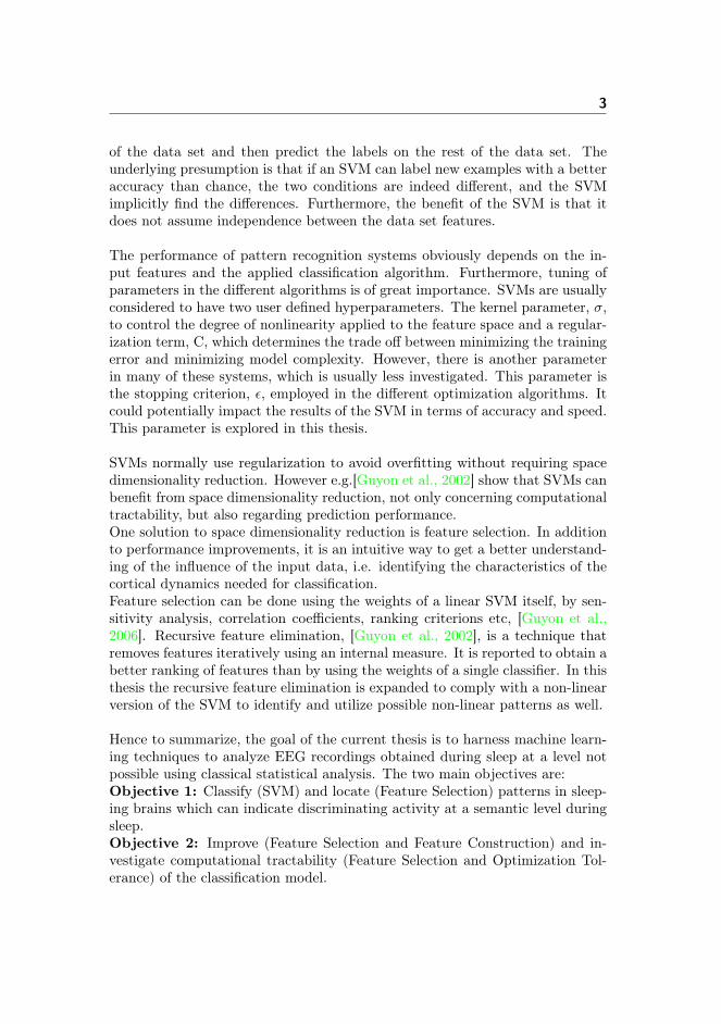
The performance of pattern recognition systems obviously depends on the in-put features and the applied classification algorithm. Furthermore, tuning ofparameters in the different algorithms is of great importance. SVMs are usuallyconsidered to have two user defined hyperparameters. The kernel parameter, σ,to control the degree of nonlinearity applied to the feature space and a regular-ization term, C, which determines the trade off between minimizing the trainingerror and minimizing model complexity. However, there is another parameterin many of these systems, which is usually less investigated. This parameter isthe stopping criterion, ε, employed in the different optimization algorithms. Itcould potentially impact the results of the SVM in terms of accuracy and speed.This parameter is explored in this thesis.
SVMs normally use regularization to avoid overfitting without requiring spacedimensionality reduction. However e.g.[Guyon et al., 2002] show that SVMs canbenefit from space dimensionality reduction, not only concerning computationaltractability, but also regarding prediction performance.One solution to space dimensionality reduction is feature selection. In additionto performance improvements, it is an intuitive way to get a better understand-ing of the influence of the input data, i.e. identifying the characteristics of thecortical dynamics needed for classification.Feature selection can be done using the weights of a linear SVM itself, by sen-sitivity analysis, correlation coefficients, ranking criterions etc, [Guyon et al.,2006]. Recursive feature elimination, [Guyon et al., 2002], is a technique thatremoves features iteratively using an internal measure. It is reported to obtain abetter ranking of features than by using the weights of a single classifier. In thisthesis the recursive feature elimination is expanded to comply with a non-linearversion of the SVM to identify and utilize possible non-linear patterns as well.
Hence to summarize, the goal of the current thesis is to harness machine learn-ing techniques to analyze EEG recordings obtained during sleep at a level notpossible using classical statistical analysis. The two main objectives are:Objective 1: Classify (SVM) and locate (Feature Selection) patterns in sleep-ing brains which can indicate discriminating activity at a semantic level duringsleep.Objective 2: Improve (Feature Selection and Feature Construction) and in-vestigate computational tractability (Feature Selection and Optimization Tol-erance) of the classification model.

4 Introduction
The thesis is organized as follows. The physiological background and the exper-iment used for the data acquisition are presented in Chapter 2. The SVM andthe algorithm for solving it will be derived in Chapter 3. The SVM is enhancedfor the current setting by feature selection schemes introduced in Chapter 4.Considerations related to parameter tuning and model selection are presentedin Chapter 5 along with a resampling framework for evaluation of the methods.Small examples are provided to illustrate the impact of the proposed heuristics.Finally the data obtained from the experiment are analyzed in Chapter 6 usingthe presented framework. In Chapter 7 the results are discussed and extensionsare proposed before a final conclusion is provided in Chapter 8.

Chapter 2
Physiological Background
2.1 Brain Activity and EEG
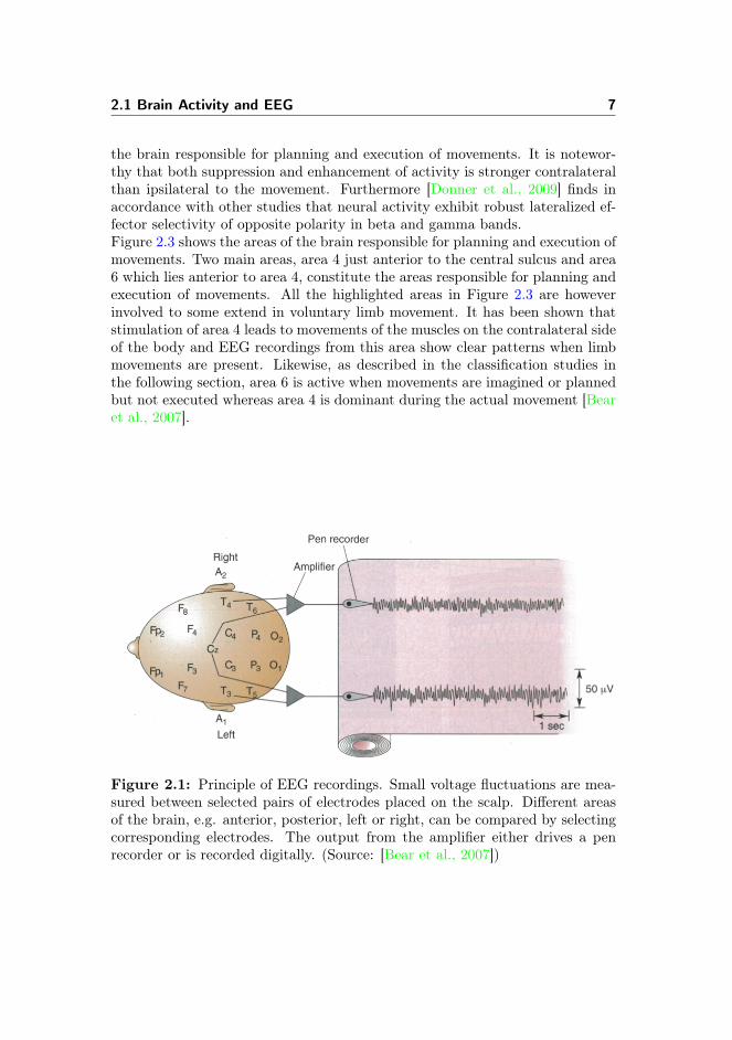
A fundamental property of the brain is the ability of groups of neurons to workin synchrony and generate oscillatory activity, [Bear et al., 2007]. Brain activ-ity and inactivity is widely studied and large-scale activity can be measured bynon-invasive techniques such as EEG, which is the recording of electrical activ-ity along the scalp, see Figure 2.1 and 2.2. In general, EEG signals have a goodtime resolution and a broad spectral content. The signals are usually describedusing the oscillatory activity in specific frequency bands, and it appears thatthe frequency of brain oscillations is negatively correlated with amplitude. Theamplitude is furthermore proportional to the number of synchronously activeneurons. This indicates that slowly oscillating cell assemblies comprise moreneurons than fast oscillating assemblies [Brown and Singer, 1993]. These fluc-tuations of field potentials from large cell assemblies are measured by electrodesthat are fixed to the outside of the scalp. Single electrodes can easily be mountedand removed, but since the EEG signal is usually recorded at many locationssimultaneously, the use of EEG caps is an advantage. In such a setup, thedistance between neighboring electrodes is usually in the range of one to a fewcentimeters.The spatial resolution of EEG is not only limited by the distance between elec-trodes, [Nunez and Srinivasan, 2006]. EEG recordings suffer from the fact that

6 Physiological Background
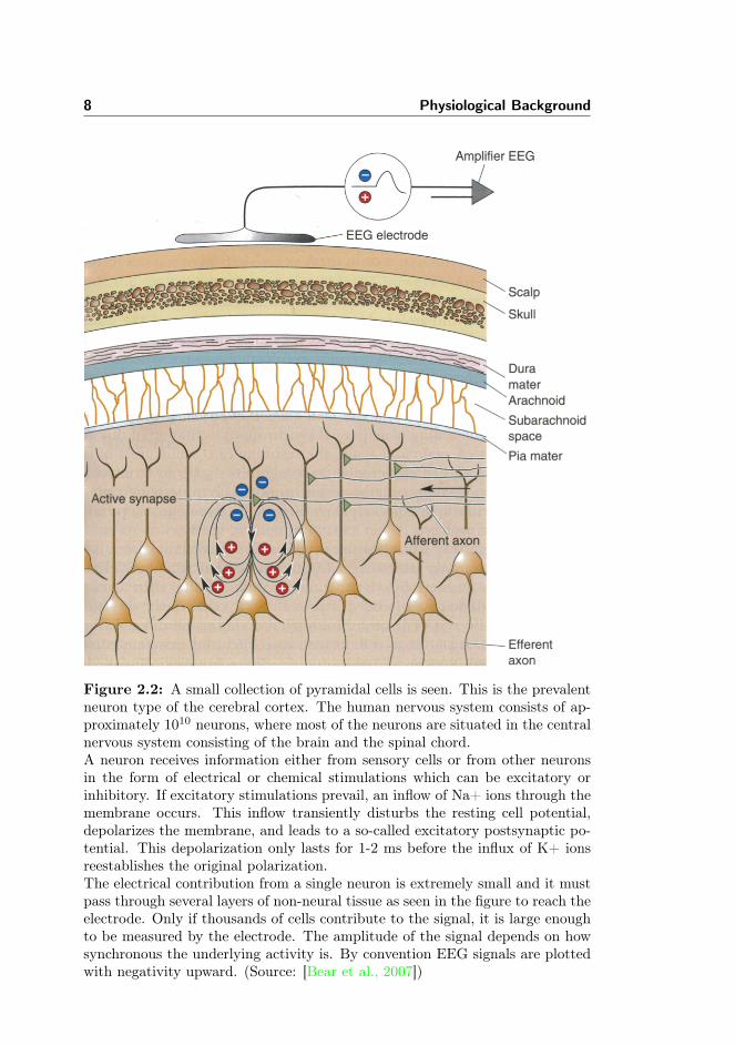
the electric signal has to pass through the intra-cerebral liquor, the meninges,the skull bone, and the skin, see Figure 2.2. These layers act as a low-passfilter to the electrical fields and act as a spatial low-pass filter as well. EEG isfurthermore very prone to so-called artifacts. Artifacts are signal componentspicked up by EEG electrodes that are not caused by neural activity and canbe so strong in amplitude that interesting signals are not detectable any more.The fact that artifacts are picked up with highest intensity at electrodes closestto their origin can help to identify them. Typical artifacts in EEG comprise:muscle activity, movements of the eyeball, eye blinks and exterior signal sources.Most artifacts however, can be controlled by proper instruction of the subjectsby using additional control electrodes close to possible artifact locations and byproper frequency filtering of the recorded signals, [Nunez and Srinivasan, 2006].[Berger, 1929] discovered the oscillatory behavior and described the commonlyoccurring alpha activity (8 -13 Hz) after his invention of EEG around 1930. Itcan be detected from the occipital lobe during relaxed wakefulness and increaseswhen the eyes are closed. Later defined frequency bands are delta (1 - 4 Hz),theta (4 - 8 Hz), beta (13 - 30 Hz) and gamma (> 30 Hz). Generally oscillationsin the beta band and above indicate an activated cortex [Bear et al., 2007]. Theexact definitions of the frequency ranges are varying slightly in the literature,especially the transition from beta to gamma is defined over a broader range,see e.g. [Nunez and Srinivasan, 2006, Pfurtscheller and Lopes da Silva, 1999].It has been shown that several kinds of events can induce time-locked changesin the oscillatory activity of ensembles of neurons or neural networks. Thesechanges are commonly referred to as event-related potentials, ERP. Averagingtechniques are commonly used to detect ERPs since these will enhance thesignal-to-noise ratio. The underlying assumption is that the brain signal has arelatively fixed time-delay to the stimulus and other ongoing activity behaves asadditive noise. This is however just a simplification of the real condition. Certainevents are indeed time-locked but not phase-locked and can either desynchro-nize or even block the present alpha activity. These types of changes can notbe extracted by simple averaging methods, but may be detected by frequencyanalysis [Pfurtscheller and Lopes da Silva, 1999]. These kind of phenomenawhere power in a given frequency band is either increased or decreased may beviewed as an increase or decrease in synchrony of the underlying neural network.It is referred to as event-related synchronization, ERS, [Pfurtscheller, 1992] andevent-related desynchronization, ERD, [Pfurtscheller, 1977].[Pfurtscheller and Lopes da Silva, 1999] propose that ERPs reflect changes inafferent activity in the cortical neurons and ERD/ERS reflect changes in theactivity of local interactions between main neurons and interneurons.[Pfurtscheller and Lopes da Silva, 1999] and [Donner et al., 2009] summarizesfrom several studies how rhythmic neural activity carries information about sen-sory stimuli, cognitive processes, or motor tasks. Limb movements especiallyare reported to be accompanied by suppression of low-frequency activity andenhancement of high frequency activity in motor cortex, which is the part of
2.1 Brain Activity and EEG 7
the brain responsible for planning and execution of movements. It is notewor-thy that both suppression and enhancement of activity is stronger contralateralthan ipsilateral to the movement. Furthermore [Donner et al., 2009] finds inaccordance with other studies that neural activity exhibit robust lateralized ef-fector selectivity of opposite polarity in beta and gamma bands.Figure 2.3 shows the areas of the brain responsible for planning and execution ofmovements. Two main areas, area 4 just anterior to the central sulcus and area6 which lies anterior to area 4, constitute the areas responsible for planning andexecution of movements. All the highlighted areas in Figure 2.3 are howeverinvolved to some extend in voluntary limb movement. It has been shown thatstimulation of area 4 leads to movements of the muscles on the contralateral sideof the body and EEG recordings from this area show clear patterns when limbmovements are present. Likewise, as described in the classification studies inthe following section, area 6 is active when movements are imagined or plannedbut not executed whereas area 4 is dominant during the actual movement [Bearet al., 2007].
Figure 2.1: Principle of EEG recordings. Small voltage fluctuations are mea-sured between selected pairs of electrodes placed on the scalp. Different areasof the brain, e.g. anterior, posterior, left or right, can be compared by selectingcorresponding electrodes. The output from the amplifier either drives a penrecorder or is recorded digitally. (Source: [Bear et al., 2007])
8 Physiological Background
Figure 2.2: A small collection of pyramidal cells is seen. This is the prevalentneuron type of the cerebral cortex. The human nervous system consists of ap-proximately 1010 neurons, where most of the neurons are situated in the centralnervous system consisting of the brain and the spinal chord.A neuron receives information either from sensory cells or from other neuronsin the form of electrical or chemical stimulations which can be excitatory orinhibitory. If excitatory stimulations prevail, an inflow of Na+ ions through themembrane occurs. This inflow transiently disturbs the resting cell potential,depolarizes the membrane, and leads to a so-called excitatory postsynaptic po-tential. This depolarization only lasts for 1-2 ms before the influx of K+ ionsreestablishes the original polarization.The electrical contribution from a single neuron is extremely small and it mustpass through several layers of non-neural tissue as seen in the figure to reach theelectrode. Only if thousands of cells contribute to the signal, it is large enoughto be measured by the electrode. The amplitude of the signal depends on howsynchronous the underlying activity is. By convention EEG signals are plottedwith negativity upward. (Source: [Bear et al., 2007])

2.1 Brain Activity and EEG 9
Figure 2.3: The areas of the cerebral cortex related to planning and executionof voluntary movements. Area 4 is the primary motor cortex and area 6 consti-tutes the premotor cortex involved in planning of movements. (Source: [Bearet al., 2007])
10 Physiological Background
2.1.1 Classification Studies
[Pfurtscheller et al., 2006] present a classification study of four motor imagerytask and concludes that the discrimination improved when ERD end ERS pat-terns were induced in at least one or two tasks. The most important electrodepositions for the classification are found to be C3, C4, and Cz of the interna-tional 10-20 system, see Figure 2.5. Furthermore an optimal spatial filteringreveals electrodes in the neighborhood of C3 and C4 to be the most impor-tant. They finally conclude there is a great inter- and intra-subject variabilityconcerning the reactivity of upper mu rhythm (9-13 Hz), which is the typicalrhytmic activity exhibited by motor cotical areas at rest.[Morash et al., 2008] use neural signals preceding movement and motor imageryto predict which of the four movements/motor imageries is about to occur, andto access this utility for BCI applications [Crone et al., 1998].Within BCI applications machine learning techniques are widely used in connec-tion with EEG recordings,[Blankertz et al., 2004, Lotte et al., 2007, Lal et al.,2004]. [Lotte et al., 2007] review classification algorithms used in a BCI set-ting and find that especially the support vector machine performs well. Usingsimilar techniques to analyze experimental data in an EEG framework is lesswidespread whereas they are commonly used to analyze neuroimaging data infMRI settings [Pereira et al., 2009, Haynes and Rees, 2006, Norman et al., 2006].[Cruse et al., 2012] and [Cruse et al., 2011] investigate motor imagery tasks in agroup of patients in the minimally conscious state and vegetative state using alinear SVM and find robust responses in some cases. They use artifact rejected,downsampled EEG signals recorded over the motor cortex and calculate logpower values at every time step in four frequency bands ranging from 7-30 Hz.60 to 203 trials contribute to each subjects single-trial analysis and accuraciesin the range 38-78 % are obtained for the two-class analysis.
2.2 The Sleeping Brain
EEG signals change dramatically during sleep and show a transition from fasterto increasingly slower frequencies. The spectral content is therefore one of themeasures used to characterize different sleep stages.Sleep has several very distinct phases but can overall be characterized by twomain stages, the the Rapid Eye Movement, REM, and non-REM sleep discoveredin the 50’s by [Aserinsky and Kleitman, 1953]. The non-REM is characterizedby high voltage and slow synchronized EEG rhythms whereas the REM sleepis characterized by desynchronized, fast and low voltage signals. When falling
2.2 The Sleeping Brain 11
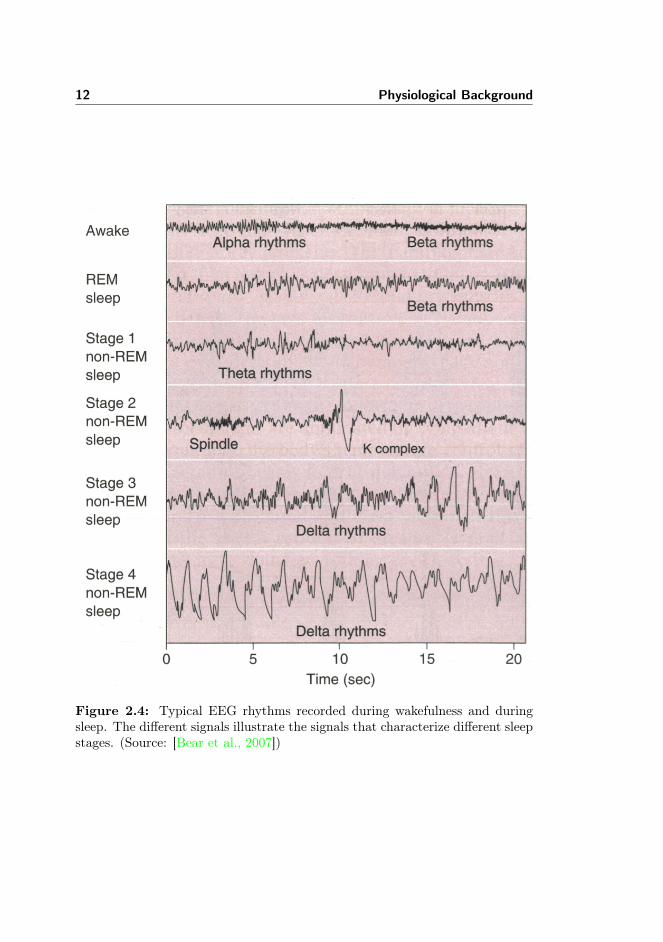
asleep the EEG alpha rhythms of relaxed wakefulness become less regular anddecline along with the eyes making slow, rolling movements. This is the firstof four stages in the non-REM sleep [Bear et al., 2007], see Figure 2.4, and isalso referred to as the drowsiness period. The second stage (light sleep) usu-ally enters after a few minutes and lasts 5-15 minutes. This stage is slightlydeeper and usually considered to be the actual onset of sleep. It is character-ized by occasional sleep spindles and K-complexes. Sleep spindles are longerlasting oscillatory brain activity in the 8-14 Hz domain whereas the K-complexis a brief high-amplitude sharp wave, see Figure 2.4. The K-complex can oc-cur spontaneously but also in response to e.g. auditory stimuli [Roth et al.,1956] and is often followed by spindles. Around actual sleep onset and beforeK-complexes and spindles occur, vertex sharp waves can be observed. They aresmall spike-like positive discharges that occur spontaneously or in response tosensory stimuli, [Rodenbeck et al., 2006]. Stage 3 (deep sleep) show large ampli-tude slow delta waves and sleep spindles gradually disappear as sleep becomesdeeper. Stage 4 (very deep sleep) is the deepest of the four stages with largedelta waves of 2 Hz or less. After stage 4 sleep lightens again and ascends tostage 2 from where it enters a brief period of REM sleep with fast beta rhythms.Physically, the REM sleep is characterized by rapid eye movements, rapid andirregular heart rate and breathing, increased blood pressure and the musclesof the body are virtually paralyzed. During a night the brain cycles throughthe different stages and generally moves towards more REM sleep as the nightprogress, [Bear et al., 2007]. Newer publications, e.g. [Iber, 2007], revise thisclassical view slightly with new class definitions and introduction of micro awak-enings and deepening of sleep within sleep stages.
2.2.1 Processing During Sleep
During sleep external stimuli are processed to some extent. The fact that peo-ple are more easily awoken by presentation of their own name and mother’s bytheir baby’s cry is a clear indication that relevant external stimuli do get someattention, [Hennevin et al., 2007, Oswald et al., 1960, Formby, 1967, Burtonet al., 1988, Bruck et al., 2009]. Another indication of the processing of externalstimuli is observed from the phenomenon that external stimuli can be incorpo-rated in dreams [Kramer et al., 1982].[Edeline et al., 2000] show for the guinea pig that auditory messages sent bythalamic cells to cortical neurons are reduced but preserved both in terms ofrate and frequencies, which indicate that the messages sent to cortical cells arenot deprived of relevant information and can explain how processing of relevantstimuli is possible during sleep. There is hence also evidence of maintainedcortical responsiveness to auditory stimuli during REM and non-REM sleep in
12 Physiological Background
Figure 2.4: Typical EEG rhythms recorded during wakefulness and duringsleep. The different signals illustrate the signals that characterize different sleepstages. (Source: [Bear et al., 2007])
2.2 The Sleeping Brain 13
both humans and animals, [Hennevin et al., 2007].Human ERP studies of response to external auditory stimuli, such as one’s ownname, [Atienza et al., 2001], indicate that auditory information processing ispossible though it is affected differently during the different stages of sleep.The P300 effect is an ERP component showing a positive deflection (relative toreference electrode) in voltage with a latency of 250 to 500 ms, which duringwakefulness is evoked in the process of decision making. During sleep, studies ofthe P300 component indicate that discriminating processes occur though shape,latency and amplitude compared to the normal P300 component is different[Hennevin et al., 2007, Atienza et al., 2001, Perrin, 2004, Perrin et al., 1999], atleast during early sleep stages and REM sleep. Compelling are also ERP studieswhich show that the N400 effect appears from word associations during bothREM and early stages of non-REM sleep [Brualla et al., 1998, Ibáñez et al.,2008, Bastuji et al., 2002]. The N400 is a negative potential (relative to refer-ence electrode) seen in the EEG which peaks around 400 ms post-stimulus inresponse to a wide array of meaningful or potentially meaningful stimuli such asauditory words. However, it is a rather automatic mechanism [Federmeier andKutas, 2009, Kutas and Federmeier, 2011], but manipulations that affect theextent to which attention is allocated to N400-eliciting stimuli do influence thesize of N400 effects. Whether processes indexed by the N400 require awarenesshas been debated for decades, but experiments suggest that N400 effects canbe obtained even when manipulations are incidental to the task and when thestimuli themselves elicit little conscious awareness, e.g. during sleep.At another level, [Antony et al., 2012] recently showed that a partly auditorytask learned during wakefulness can be promoted during sleep, which is anotherindication that more active processing takes place.Hence there are various indications that during sleep, auditory stimuli are inte-grated at a semantic level, but clearly further evidence and investigation of thelevel of cognitive processing is needed. Whether sleep involves deeper processingnot only at a semantic level but all the way "up" to the preparation of task-relevant responses remains unclear. According to [Nofzinger et al., 2002, Ma-quet et al., 2000, Manganotti et al., 2004] the relative cortical activity in sleepand awakening of motor cortex indicates that motor cortex is not fully deacti-vated during sleep. However, it does remain a question whether cortical motorprocesses are active during sleep. And it is indeed a question posing certainchallenges to investigate since the initialization of a new task-set might provedifficult during sleep stages, because the prefrontal regions dealing with execu-tive functions are particularly suppressed in comparison to other cortical regions[Muzur et al., 2002, Maquet et al., 2000]. This is somewhat addressed in the ex-periment described in Section 2.3, which is the background of this thesis. Herean induction strategy is used as an approach for the study of non-consciousperception. The results presented in the following are obtained during the earlystages of non-REM sleep and hence it remains to investigate whether it gener-alize to other sleep stages including REM sleep.
14 Physiological Background
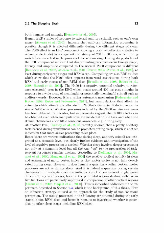
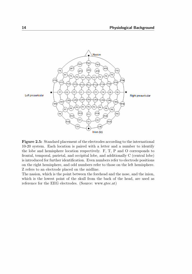
Figure 2.5: Standard placement of the electrodes according to the international10-20 system. Each location is paired with a letter and a number to identifythe lobe and hemisphere location respectively. F, T, P and O corresponds tofrontal, temporal, parietal, and occipital lobe, and additionally C (central lobe)is introduced for further identification. Even numbers refer to electrode positionson the right hemisphere, and odd numbers refer to those on the left hemisphere.Z refers to an electrode placed on the midline.The nasion, which is the point between the forehead and the nose, and the inion,which is the lowest point of the skull from the back of the head, are used asreference for the EEG electrodes. (Source: www.gtec.at)
2.3 Experimental Setup 15
2.3 Experimental Setup
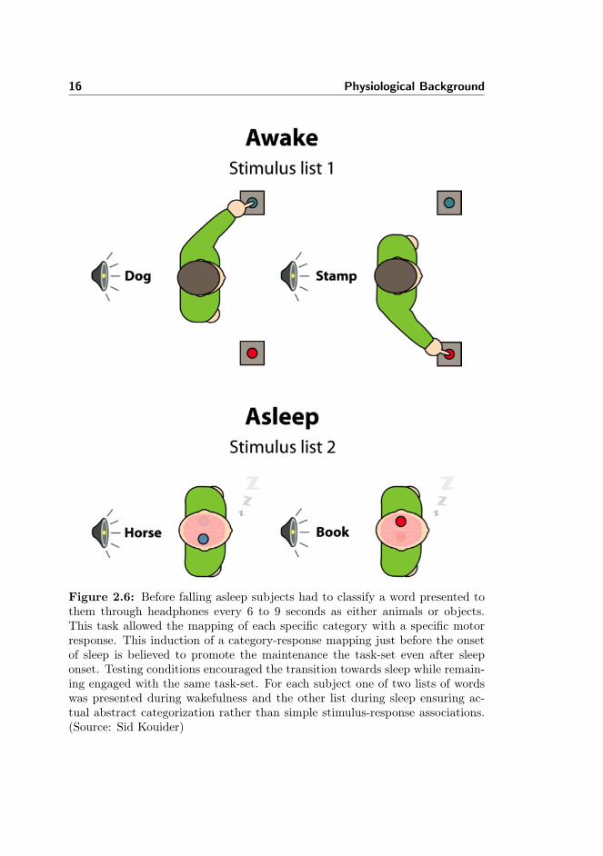
The depth of unconscious cognitive processing can be investigated at variouslevels and using various approaches. More specifically the present thesis dealswith the question of whether there is maintained some semantic processing inthe unconscious state of sleep and if it is possible to show that auditory stimulipresented to the sleeping subject can reach higher levels of processing.To answer the question, data from an experiment conducted by Dr. Sid Kouiderat Laboratoire de Sciences Cognitives et Psycholinguistique, École NormaleSupérieure is analyzed. In this study it was tested if an association betweena semantic category and a specific motor response learned during wakefulnesscan be maintained in sleep. More specifically, it was tested whether a learnedmotor mapping association between a lateralized motor action and specific se-mantic category is preserved during early sleep stages. The experiment relieson an induction strategy to overcome the problem of learning a completely newtask-set during sleep. Subjects were presented a task-set while they were stillawake and then tested whether this task-set was maintained after subjects fellasleep, see Figure 2.6. In this section the experimental setup will be describedbriefly.
2.3.1 Procedure
Subjects were instructed to do a categorization of spoken words by pressinga button with their left or right hand depending on corresponding semanticcategory, i.e. animals or objects, see Figure 2.6. While doing the classificationsubjects were lying in a comfortable chair in a dark room with their eyes closedto encourage the transition towards sleep. The auditory stimuli was presentedin headphones and subjects were instructed that they could fall asleep anytimeduring the experiment but were also asked not to stop responding voluntarilyto easier fall asleep. When the subjects were assessed to be asleep a new listof words was introduced. This new list had the same properties, see Section2.3.2, as the list presented during sleep, but was introduced to test for genuinesemantic effects rather than simple stimulus-response associations [Kouider andDehaene, 2007].
2.3.2 Stimuli
The spoken words used as stimuli were selected from the CELEX lexical database(Linguistic Data Consortium, University of Pennsylvania). There were 48 names
16 Physiological Background
Figure 2.6: Before falling asleep subjects had to classify a word presented tothem through headphones every 6 to 9 seconds as either animals or objects.This task allowed the mapping of each specific category with a specific motorresponse. This induction of a category-response mapping just before the onsetof sleep is believed to promote the maintenance the task-set even after sleeponset. Testing conditions encouraged the transition towards sleep while remain-ing engaged with the same task-set. For each subject one of two lists of wordswas presented during wakefulness and the other list during sleep ensuring ac-tual abstract categorization rather than simple stimulus-response associations.(Source: Sid Kouider)
2.3 Experimental Setup 17
of objects and 48 names of animals. Half were monosyllabic and the other halfdisyllabic, with animal and object names matched as closely as possible in termsof combined (spoken and written) log lemma frequencies, as confirmed by an in-dependent t-test (p > 0.10). Additionally, words within the two categories werematched in a pair-wise fashion regarding their phonological properties: eachobject name was matched with a similar animal name (for example "quilt" wasmatched with "quail"), ensuring that animal and object names could not be dif-ferentiated in terms of phonological properties. The words were tape-recordedby a female voice and digitized. Durations of the resulting stimuli ranged from357 to 800 ms. Two lists of 48 stimuli each were produced, one for the awakeningperiod and the other for the sleeping period.
2.3.3 Sleep Assessment
Sleep onset was assessed both online and offline. During the experiment subjectswere assessed to be asleep when showing no overt response for at least twominutes of stimulation and if the EEG showed sleep markers before and afterthe presentation of each word, i.e. vertex sharp waves, regular spontaneous andevoked K-complexes, sleep spindles, and an overall reduction of fast, alpha/betarhythms in favor of slower delta/theta rhythms, cf. Section 2.2. After theexperiment was finished, this was verified offline, and ambiguous epochs wereexcluded from the analysis.
2.3.4 Subjects
18 out of 47 subjects fell asleep for at least 9 consecutive minutes and wereincluded in this study. Of these, 6 were women and 12 were men in the agerange 18-30-years-old. They were all healthy native English speakers, right-handed and reported no auditory, neurological or psychiatric alterations. Onlyself reported easy sleepers [Johns et al., 1991] were chosen for the experimentto increase the probability that subjects would fall asleep. Subjects were alsoasked to avoid exciting substances as coffee, and to sleep 1-2 hours less thanusual the night preceding the experiment. They signed a written consent andwere paid for their participation.

18 Physiological Background
2.3.5 EEG Equipment
The electroencephalogram was continuously recorded from 64 Ag/AgCl elec-trodes mounted on an electrode cap (Easycap, Falk Minow Services, Herrsching-Breitbrunn, Germany) using SynAmps amplifiers (NeuroScan Labs, Sterling,VA), with Cz as a reference. The impedance for electrodes was kept below 6kΩ. Data were acquired with a sampling rate of 500 Hz, and then down sampledat 250 Hz. An electrooculogram (EOG) was recorded through electrodes placedabove and below the right eye (vertical) and at the outer canthi (horizontal).Amplifier band pass was 0.1-100 Hz.

Chapter 3
Support Vector Machines
Statistical learning theory [Vapnik, 2006, Vapnik, 2000, Vapnik, 1998] providesthe theoretical basis for machine learning and Support Vector Machines, SVM.It deals with the problem of inferring a predictive function based on empiricaldata using concepts from the fields of statistics and functional analysis.SVMs have developed in several directions such that they have applications bothwithin regression estimation as well as single-class and multi-class classification.This thesis deals with the formulation dealing with two-class pattern recognitionin the non-linear version [Boser et al., 1992, Cortes and Vapnik, 1995, Vapnik,1998].The foundation of the SVM is the separating hyperplane. From this an optimalmargin hyperplane can be defined and extended to the case where data are non-separable. Furthermore the optimal margin hyperplane can be generalized to anon-linear version where it is computed in a feature space non-linearly relatedto the input space. The following review is inspired by [Schölkopf and Smola,2002, Bishop, 2007].

20 Support Vector Machines
3.1 The Learning Setting
Suppose m observations, where each observation belongs to only one of twodifferent classes, are given. Each observation consists of a pattern vector xi ∈X , i = 1, ...,m and the associated class label yi, which for mathematical conve-nience is labelled by either +1 or −1 in the simple binary classification problem.In the present thesis this corresponds to the classification of words belongingto one of two classes. In the frame of mathematical learning the goal is to beable to generalize to unseen data, i.e. for a new x ∈ X it is possible to predictthe corresponding y ∈ ±1. Again in the present thesis, given an EEG epochrecorded during auditory stimulation, it is possible to predict the word class. Inthe following it is assumed that there exists some unknown but fixed probabilitydistribution P(x,y) from which these data are drawn and the data are assumedi.i.d. For all x ∈ X we want to estimate a function f : X → ±1.
3.2 Separating Hyperplanes
If the pattern vectors are given in a dot product space x ∈ H, then any hyper-plane can be written as
x ∈ H|〈w,x〉+ b = 0, w ∈ H, b ∈ <, (3.1)
where w is an orthogonal vector to the hyperplane, see also Figure 3.1.
The dot product is a simple similarity measure, since it represents geometricconstructions that can be formulated in terms of angles, lengths and distances.Later a kernel function, k, will be introduced since it turns out that in manyproblems the dot product is not sufficiently general. However, both the dotproduct and kernels gives a way to characterize similarity in two patterns ge-ometrically and hence the ability to construct learning algorithms using linearalgebra and analytic geometry. In both cases the space H is called a featurespace.If the hyperplane is scaled such that the point closest to the hyperplane has adistance of 1
‖w‖ , the hyperplane is said to be canonical and much freedom inchoosing a hyperplane is gone. Nevertheless, it is still possible to choose both(w, b) and (−w,−b). Without class labels it is not possible to distinguish thesehyperplanes. For pattern recognition problems they are different as they make
3.2 Separating Hyperplanes 21
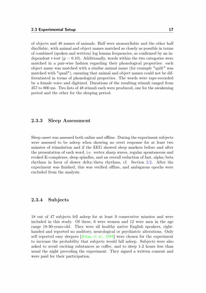
Figure 3.1: The SVM "learns" a hyperplane which gives the best separation oftwo classes. The figure shows a 2-dimensional classification problem where reddots correspond to the class label +1 and green dots corresponds to the classlabel -1.
opposite class assignments using the two inversely correlated decision functions
fw,b : H → ±1x 7→ fw,b(x) = sgn(〈w,x〉+ b). (3.2)
From this it is clear how a separating hyperplane can be constructed if the dataare separable, i.e. two disjoint sets with corresponding different class labels.In creating learning algorithms it proves useful to define the margin as well. Themargin is defined as the perpendicular distance between the decision boundaryand the closest data point, hence for a hyperplane, the geometric margin of thepoint (x, y) ∈ H × ±1 is defined as
ρ(w,b)(x, y) := y(〈w,x〉+ b)/‖w‖, (3.3)
and the minimum value
ρ(w,b) := mini=1,...,m
ρ(w,b)(xi, yi), (3.4)
is the geometrical margin, or just the margin, of (x1, y1), . . . , (xm, ym).For a correctly classified point (x, y) the margin is the distance from x to the hy-perplane and for a misclassified point the margin gives a negative distance. This

22 Support Vector Machines
can be seen from the fact that for the canonical hyperplane considered the mar-gin is 1/‖w‖ and the length of the weight vector is 1. Hence it is the projectionof x onto the direction orthogonal to the hyperplane. The idea behind SVMs isto choose a decision boundary for which the margin of the separating hyperplaneis maximized. The intuition behind this is that a large margin will give the op-timal separation of the data. Furthermore, since the observed data is assumedto have been generated by the same underlying process it seems reasonable toassume that new observations will lie close (inH) to one of the training patterns.
3.3 Optimal Margin Hyperplanes
An important property of support vector machines is that the determination ofthe model parameters eventually corresponds to a convex optimization problem,hence any local solution is also a global optimum. Finding the optimal separat-ing hyperplane (maximum margin) is the heart of the support vector machineand it basically boils down to optimizing the parameters w and b in order tomaximize the decision boundary.For the canonical hyperplane all points will satisfy yi(〈xi,w〉 + b) ≥ 1 and thedecision boundary is optimized when ‖w‖−1 is maximized. Hence, for a linearlyseparable set of training data the optimal separating hyperplane can be foundfrom the following quadratic optimization problem
minw∈H,b∈<
τ(w) =1
2‖w‖2 (3.5)
subject to: yi(〈xi,w〉+ b) ≥ 1 ∀ i = 1, ...,m. (3.6)
Solving this primal problem will result in (w, b) with the largest possible ge-ometric margin with respect to the training set. The dual problem however,can give some additional insight and it is here the foundation of the SVM isfound. The Lagrangian of the inequality constrained primal convex quadraticoptimization problem is given by
L(w, b,α) =1
2‖w‖2 −
m∑i=1
αi(yi(〈xi,w〉+ b)− 1), (3.7)
where αi ≥ 0 are the Lagrange multipliers.The corresponding Karush-Kuhn-Tucker, KKT, optimality conditions, [Nocedaland Wright, 1999] are both necessary and sufficient conditions for optimalitysince both the objective function and the inequality constraints are continuouslydifferentiable convex functions.To obtain the same solution as to the primal problem, the Lagrangian must be

3.3 Optimal Margin Hyperplanes 23
minimized with respect to w and b and maximized with respect to αi, hence thesolution is found at a saddle point. Minimizing the Lagrangian with respect tow and b yields two conditions
∂
∂wL(w, b,α) = 0 (3.8)
∂
∂bL(w, b,α) = 0, (3.9)
which implies that
m∑i=1
αiyi = 0 (3.10)
w =
m∑i=1
αiyixi. (3.11)
From 3.11 it can furthermore be seen that the unique solution vector (due toconvexity) has an expansion only in terms of the training data. If 3.11 is pluggedinto the Lagrangian 3.7, we obtain
L(w, b,α) =
m∑i=1
αi −1
2
m∑i,j=1
αiαjyiyjxTi xj − bm∑i=1
αiyi, (3.12)
which can be reduced using 3.10 such that
L(w, b,α) =
m∑i=1
αi −1
2
m∑i,j=1
αiαjyiyjxTi xj . (3.13)
Combined with the constraints, we have the dual form of the primal optimizationproblem
maxα∈<m
m∑i=1
αi −1
2
m∑i,j=1
αiαjyiyj〈xi,xj〉 (3.14)
subject to: αi ≥ 0, i = 1, ...,m (3.15)m∑i=1
αiyi = 0. (3.16)
This is the foundation of the SVM algorithm, written only in terms of the innerproduct between points in the input feature space and the parameters (Lagrangemultipliers) αi. For every training point there is a Lagrange multiplier αi. Atthe solution, those points, xi for which αi > 0 are called support vectors andthey lie exactly on the margin. All other training points have αi = 0 and areirrelevant as they do not appear in (3.11).

24 Support Vector Machines
Now suppose the models αi’s are found using a training set, and we wish tomake a prediction at a new input x. We would then calculate 〈w,x〉 + b, andpredict y = 1 if and only if this quantity is bigger than zero. But using (3.11) ,this quantity can also be written
wTx + b = (
m∑i=1
αiyixi)Tx + b =
m∑i=1
αiyi〈xi,x〉+ b. (3.17)
Hence the prediction only depends on the inner product between the new pointx and the points in the training set. Moreover, the αi’s will all be zero exceptfor the support vectors. Thus, many of the terms in the sum will be zero, andonly the inner products between x and the support vectors (of which there isoften only a small number) need to be calculated in order to calculate (3.17)and make a prediction using the sgn function.
3.4 Soft Margin Optimal Hyperplanes
The classifier considered so far is ideally suited for linearly separable data with-out outliers. However, in practice data is rarely in that condition, and thealgorithm must be adjusted to work for non-separable data sets and to be lesssensitive to outliers. To allow some of the training points to be misclassified,the optimization problem can be reformulated by introducing slack variables foreach training point, ξi ≥ 0, i = 1, ...,m and relax the separation constraints 3.6such that
yi(〈xi,w〉+ b) ≥ 1− ξi i = 1, ...,m. (3.18)
Correctly classified training points that are either on the margin or on the correctside of the margin yields ξi = 0. Points that lie inside the margin, but on thecorrect side of the decision boundary have 0 < ξi ≤ 1, and misclassified datapoints on the wrong side of the decision boundary yields ξi ≥ 1, see Figure3.1. This allows the constraints to be satisfied by making ξi large enough as itrelaxes the hard margin constraint to give a "soft" margin and allows some of thetraining set data points to be misclassified. However, it is necessary to penalizelarge values of ξi in order not to obtain the trivial solution where all ξi’s arelarge. This can be done by including the slack variables in the objective functionof (3.5), hence our goal is now to maximize the margin while penalizing points

3.5 The Non-linear Support Vector Machine for Non-separable Data 25
that lie on the wrong side of the margin. This can be formulated as follows
minw∈H,b∈<
τ(w) =1
2‖w‖2 + C
m∑i=1
ξi (3.19)
subject to: yi(〈xi,w〉+ b) ≥ 1− ξi i = 1, ...,m (3.20)ξi ≥ 0 i = 1, ...,m, (3.21)
where the parameter C > 0 is similar to a regularization coefficient because itcontrols the trade-off between minimizing training errors (corresponding to thenon-zero slack variables and the corresponding penalty) and controlling modelcomplexity (maximizing margin). The original formulation can for separabledata be recovered in the limit where C →∞. The selection of the C parameterhas proven to be rather unintuitive, and there is no obvious a priory way ofselecting it, other than searching a wide range of values, [Shawe-Taylor andCristianini, 2004]. As for the original primal problem (3.5) - (3.6) it is possibleto obtain a dual formulation. The Lagrangian is given by
L(w, b, ξ,α, r) =1
2‖w‖2 + C
m∑i=1
ξi −m∑i=1
αi[yi(〈xi,w〉+ b)− 1 + ξi]−m∑i=1
riξi,
(3.22)
where ξi ≥ 0 and ri ≥ 0 are the corresponding Lagrange multipliers. Followingthe same procedure as previous the dual formulation can be obtained
maxα∈<m
m∑i=1
αi −1
2
m∑i,j=1
αiαjyiyj〈xi,xj〉 (3.23)
subject to: 0 ≤ αi ≤ C, i = 1, ...,m (3.24)m∑i=1
αiyi = 0, (3.25)
where the only change turns out to be an upper bound on the αi’s, these con-straints are known as box constraints. Predictions for new data points are doneusing 3.17.
3.5 The Non-linear Support Vector Machine forNon-separable Data
A very important extension of the presented classifier comes with the intro-duction of kernels. Everything in the setting so far deals with classification of

26 Support Vector Machines
more or less linearly separable data. In the following kernels are introduced tonon-linearly transform the input data, now denoted x1, ..., xm ∈ X , using a mapφ : xi → xi into a high-dimensional feature space and do the linear separationthere. In practice it requires only small modifications of the presented formula-tion and the transformation leads to a much more powerful classification tool.As with the dot product, the kernel function is used as a similarity measure,and a large class of kernels actually admit a dot product representation in afeature space. Kernels can in general be regarded as generalized dot productsand any dot product is in fact a kernel. More formally the class of kernels kthat correspond to a dot product in a feature space H via a map φ that satisfies
φ : X → Hx→ x := φ(x), (3.26)
then
k(x, xi) = 〈φ(x),φ(xi)〉. (3.27)
There are no constraints on the structure of the domain X other than it needsto be a non-empty set. Since it is possible to compare similarities between non-vectorial objects such as strings [Haussler, 1999] it makes kernels applicable insituations where vectorial representation is not readily available and expands thefield of kernel methods. In this thesis however, only vectorial data is considered.The term kernel originates from the first use of this type of function in the fieldof integral operators. They were originally introduced since there are manyclasses of problems that are harder to solve in their original representations.An integral transform maps a function from its original domain into anotherdomain. Solving the equation in the target domain can be easier than in theoriginal domain. The solution can then be mapped back to the original domainusing the inverse of the integral transform.
Definition 3.1 [Polyanin and Manzhirov, 2008]A function k which gives rise to an operator Tk via(Tkf)(x) =
∫X k(x, xi)f(xi)dxi
is called the kernel of Tk.
For a kernel to be valid and describe a dot product in some feature space itgenerally needs to satisfy Mercer’s Theorem, see e.g. [Mercer, 1909, Schölkopfand Smola, 2002]. Usually Mercer’s theorem is presented in a form involvingL2 functions, but when the input data take values in Rn as in this thesis, it isequivalent to:
Theorem 3.2 (Mercer) Let K : Rn ×Rn → Rn be given.Then for K to be a valid kernel, it is necessary and sufficient that for any

3.5 The Non-linear Support Vector Machine for Non-separable Data 27
x1, ..., xm, (m < ∞), the corresponding kernel matrix is symmetric positivesemi-definite.
In continuation of Mercers Theorem, the following proposition is used:
Proposition 3.3 [Schölkopf and Smola, 2002]If k is a kernel satisfying the conditions of Mercers Theorem, we can constructa mapping φ into a space where k acts as a dot product,〈φ(x),φ(xi)〉 = k(x, xi),for almost all (except for sets of measure zero) x, xi ∈ X . Moreover, given anyε ≥ 0, there exists a map φn into an n-dimensional dot product space (wheren ∈ N depends on ε) such that|k(x, xi)− 〈φ(x),φ(xi)〉| ≤ εfor almost all (except for sets of measure zero) x, xi ∈ X .
Positive definite kernels are also called reproducing kernels [Schölkopf and Smola,2002] and can thought of as a set of dot products in another space. The repro-ducing kernel property amounts to
〈φ(x),φ(xi)〉 = k(x, xi), (3.28)
which is also the basis of the "kernel trick", which basically states that any algo-rithm formulated in terms of a positive definite kernel, k, can be reformulated toan alternative algorithm by replacing k by a new positive definite kernel k. TheReproducing Kernel Hilbert Spaces theory more precisely states which kernelfunctions correspond to a dot product and the linear spaces that implicitly areinduced by these kernel functions, see [Schölkopf and Smola, 2002].An example of this is an algorithm where the k is the dot product in the in-put domain such as the formulation of the optimal separating hyperplane. Ifthe formulation of the optimal hyperplane everything can be rewritten in termsof φ(s) instead of x and then using the kernel trick we have a way of write anonlinear operator as a linear one in a space of higher dimension
maxα∈<m
m∑i=1
αi −1
2
m∑i,j=1
αiαjyiyjk(xi, xj)
subject to: 0 ≤ αi ≤ C, i = 1, ...,m (3.29)m∑i=1
αiyi = 0,
with the corresponding decision function
f(x) = sgn
(m∑i=1
yiαik(x, xi) + b
). (3.30)

28 Support Vector Machines
For support vectors xj for which ξj = 0 the threshold b can be computed byaveraging 3.20 over all support vectors xj , since they satisfy 0 < αj < C.
3.5.1 Kernel
One function satisfying the properties described in the previous section is theRadial Basis Function, RBF, kernel. In general the RBF kernel shows someattractive properties and performs very well for a wide range of problems, see[Caputo et al., 2002]. Any continuous decision boundary can be obtained usingthe RBF kernel, but with proper parameter selection it makes the SVM behavelike a simple linear classifier, see section 5.5.1. The RBF kernel is given by
K(x, xi) = e−||x−xi||
2σ2 . (3.31)
Other kernel functions are e.g. the linear kernel, the polynomial kernel, thespline kernel, the Fourier kernel, and the Sigmoid kernel. Except for the linearkernel which is considered briefly, these are not considered further.
3.6 Numerical Optimization
As long as the kernel matrix fits the main memory of modern computers, fastand accurate solutions exist in terms of Quadratic Programming, QP, solvers.In many real life problems the kernel matrix however, is too large to make thefull problem tractable.
The Sequential Minimal Optimization, SMO, was introduced by Platt [Platt,1998], improved by [Keerthi et al., 2001] and a modified version [Fan et al., 2005]is implemented in LIBSVM [Chang and Lin, 2011] in an analogous version ofthe quadratic formulation presented in previous sections. The SMO algorithmis a widely applied approach for solving the considered QP problem as it hasdesirable properties for large-scale problems. The SMO algorithm consists inmost implementations of an analytical part for optimizing the smallest possiblesubproblem consisting of two multipliers, and a heuristic part for choosing whichtwo multipliers to optimize.

3.6 Numerical Optimization 29
3.6.1 Subset selection
The quadratic optimization problem in 3.29 is covered by the following QP
minα
1
2αTQα+ cTα
subject to Aα = d (3.32)0 ≤ α ≤ u,
which can be formulated as a convex program in a subset of the variables.Assume there exists a subset, the working set, Sw ⊂ [m] which will be usedduring optimization and a fixed set Sf = [m] \ Sw which will not be modified.Then Q, c,A, and u can be split up accordingly into the following permutationmatrices
Q =
[Qww Qfw
Qwf Qff
], c = (cw, cf ), A = [Aw, Af ], u = (uw, uf ), (3.33)
and the QP can be restated as
minαw
1
2αTwQwwαw + [cw +Qwfαf ]Tα+ [
1
2αTf Qff αf + cTf αf ] (3.34)
subject to Awαw = d−Afαf0 ≤ αw ≤ uw,
where the constant offset produced by αf is not to be considered in the actualoptimization. Solving the subset problem will lead to an improvement of thefull problem, and several heuristics have been proposed for choosing the workingset.
3.6.2 Sequential Minimal Optimization
The SMO algorithm is the extreme case of the above, where the working setonly consist of two variables
minαi, αj
1
2[α2iQii + α2
jQjj + 2αiαjQij ] + ciαi + cjαj
subject to sαi + αj = γ
0 ≤ αi ≤ Ci
0 ≤ αj ≤ Cj ,
where s ∈ ±1, Q ∈ <2x2, and ci, cj , γ ∈ < are chosen accordingly.There exist an analytic solution to this optimization problem. The following

30 Support Vector Machines
shows the derivation and finds the explicit values needed during iterations of thealgorithm. By using the equality constraint, sαi+αj = γ, it is possible to expressthe objective function only in terms of αi since αj = γ− sαi. Furthermore, dueto the constraints on αj , sαi = γ − αj , the following bound γ ≥ sαi ≥ γ − Cjapplies. Combining this with the bound on αi, 0 ≤ αi ≤ Ci, it is possible toobtain the following constraint: H ≥ αi ≥ L, where
L =
max(0, s−1(γ − Cj )) if s > 0max(0, s−1γ) o.w.
H =
min(Ci, s
−1γ) if s > 0min(Ci, s
−1(γ − Cj )) o.w.
Then, with the new bound on αi, it is possible to substitute αj = γ − sαi andthe QP can then be stated only in terms of αi as
minαi
1
2α2i (Qii +Qjj − 2sQij ) + αi(ci − scj + γQij − γsQjj )
subject to L ≤ αi ≤ H. (3.35)
By introducing the auxiliary variables
Γ = scj − ci + γsQjj − γQij (3.36)Λ = (Qii +Qjj − 2sQij ), (3.37)
the unconstrained objective function can be written as: Λ2 α
2i − Γαi. By taking
the derivative, the corresponding unconstrained minimum is obtained at αi =Λ−1Γ. To ensure that the solution is within the constrained interval αi ∈ [L,H]the unconstrained solution is cut to the interval, i.e. αi = min(max(Λ−1Γ, L), H).In the case of classification it must hold that
∑mi=1 yiαi = 0 and hence yiαi +
yjαj = yiαoldi + yjα
oldj . This gives γ := yiyjαi + αj = yiyjα
oldi + αoldj and
s = yiyj .Furthermore from (3.33) it is given that Qii = Kii, Qjj = Kjj , Qij = Qji =sKij where Kij := k(xi, xj) is the kernel matrix and hence
Λ = Kii +Kjj + 2Kij . (3.38)
To find Γ, ci and cj can be obtained from (3.34)
ci = −1 + yi
m∑l 6=i,j
αlk(xi, xl)
= yi(f(xi)− b− yi)− αiKii − αjsKij (3.39)
cj = −1 + yj
m∑l 6=i,j
αlk(xj , xl)
= yj(f(xj)− b− yj)− αiKjj − αisKij .
(3.40)

3.6 Numerical Optimization 31
Then Γ can be computed using yi = yjs
Γ =− yi(f(xi)− b− yi) + αiKii + αjsKij + yi(f(xj)− b− yj)+ αjsKjjαiKij + (αi + sαj)(Kij −Kjj
=yi((f(xj)− yj)− (f(xi)− yi)) + αiΛ. (3.41)
Plugging back into the original formulation yields the following results:If yi = yj
L = max(0, αoldi + αoldj − Cj) (3.42)
H = min(Ci, αoldi + αoldj ), (3.43)
and if yi 6= yj
L = max(0, αoldi + αoldj ) (3.44)
H = min(Ci, Cj + αoldi + αoldj ), (3.45)
then the optimal values are
αi = min(max(α, L), H) (3.46)
αj = s(αoldi − αi)− αoldj , (3.47)
where
α =
αoldi + Λ−1δ if Λ > 0−∞ if Λ = 0 and δ > 0∞ if Λ = 0 and δ < 0
,
and δ := yi((f(xj)− yj)− (f(xi)− yi)).
From the above, it can be seen that if the constrained and unconstrained so-lution are identical, i.e. αi = α, then the objective function is improved byΛ−1((f(xj)− yj)− (f(xi)− yi))2. Hence it is important to select a working setwhich makes this term large, see e.g. [Keerthi et al., 2001].
3.6.3 Stopping Criterion
As the decomposition method asymptotically approaches an optimum, it is inpractice terminated after satisfying a stopping criterion. Some methods focus onthe precision of the Lagrange multipliers αi, whereas others use the proximityof the primal and the dual objective functions [Schölkopf and Smola, 2002]. It isworth noticing that an improvement in the primal objective does not necessarilyimply an improvement in the dual and vice versa. In SMO the dual gap can

32 Support Vector Machines
fluctuate considerably. In the SMO-algorithm implemented in LIBSVM, [Changand Lin, 2011], the KKT conditions are checked to be within ε of fulfillment: Thestandard KKT conditions [Nocedal and Wright, 1999] of the dual formulation,Equation 3.32, states that if there exist a scalar, b, and two nonnegative vectorsλ and µ such that
∇f(α) + by = λ + µ (3.48)λiαi = 0, i = 1..m (3.49)
µi(C − αi) = 0, i = 1..m (3.50)λi = 0, i = 1..m (3.51)µi = 0, i = 1..m (3.52)
where ∇f(α) ≡ Qα+c is the gradient of f(α). Then a feasible α is a stationarypoint of 3.32. The conditions can be rewritten as
∇if(α) + byi ≥ 0 if αi < C (3.53)∇if(α) + byi ≤ 0 if αi > 0. (3.54)
Utilizing the fact that yi = ±1 this yields that there exists a b such that
m(α) = maxi∈Ihi(α)
−yi∇if(α) ≤ b ≤M(α) = mini∈Ilo(α)
−yi∇if(α), (3.55)
where
Ihi(α) ≡ t|αt < C, yt = 1 or αt > 0, yt = −1 (3.56)Ilo(α) ≡ t|αt < C, yt = −1 or αt > 0, yt = 1. (3.57)
Hence for an α to be feasible it must hold
m(α) ≤M(α), (3.58)
which gives the stopping condition employed in LIBSVM
m(α)−M(α) ≤ ε, (3.59)
where ε is the stopping tolerance. The SMO algorithm with the described stop-ping criterion has been shown to converge in a finite number of iterations [Chenet al., 2006, Fan et al., 2005, Keerthi and Gilbert, 2002].The time required for the SMO algorithm to converge hence depends on the de-sired accuracy of the output but also on the working set selection. The literatureinvestigating this kind of stopping tolerance for the SMO algorithm is limited,but it generally seems there is consensus that ε = 10−3 is the default value touse. [Joachims, 1999, Chang and Lin, 2011, Fan et al., 2005, Hsu and Lin, 2002]use ε = 10−3, with the general note that this is an acceptable value, though

3.6 Numerical Optimization 33
without providing any evidence except from Platt’s paper [Platt, 1998] whichstates: "Recognition systems typically do not need to have the KKT conditionsfulfilled to high accuracy: it is acceptable for examples on the positive margin tohave outputs between 0.999 and 1.001". Nevertheless, it is a very interesting pa-rameter to investigate further since it obviously is a trade-off between accuracyand computational effort.
3.6.4 Implementation
LIBSVM [Chang and Lin, 2011] is a library for SVMs written in C++. Itimplements a version of a SVM for classification problems similar to the onedescribed in the present chapter and solves the optimization problem using theSMO algorithm. LIBSVM has a compiled interface which allows all functionsto be called from MATLAB. The library is modified in this thesis to producea non-standard output used for the feature extraction algorithm described inSection 4.2.3. The code is slow since it, in addition to the suppressible outputs,produces non-suppressible outputs during every iteration. These are removedand a Matlab routine, which utilizes the SUN grid-engine cluster facilities atDTU Informatics, is written, to be able to process high-dimensional jobs in ahigh performing parallel environment.

34 Support Vector Machines

Chapter 4
Feature Extraction
Machine learning methods, including SVMs, do not necessarily work well whenapplied to raw EEG data signal segments. One of the major difficulties inbuilding a classification model based on EEG recordings is to find a good datarepresentation. Feature extraction deals with construction and selection of rel-evant and informative features.
4.1 Feature Construction
New features can be constructed to get an appropriate data representation. Ac-cording to [Guyon and Elisseeff, 2003], performance can often be improved usingfeatures derived from the original input. Building a new feature representationis also a way of incorporating domain knowledge. There are a number of genericfeature construction methods, including clustering, linear transforms of the in-put variables, e.g. Principal Component Analysis, PCA, Linear DiscriminantAnalysis, LDA, and spectral transforms e.g. Fourier, multitaper, and wavelettransforms.As described in Section 2.1, raw EEG signals are time series of voltage fluc-tuations resulting from ionic current flows within the neurons of the brain.Many applications and analyses does however, as described, generally focus onthe spectral content of EEG, i.e. the type of neural oscillations that can be

36 Feature Extraction
observed in EEG signals and it has been demonstrated numerous times thatassessing specific frequencies can often yield insights into the functional cogni-tive correlations of these signals. Hence instead of representing the data in theoriginal domain, it can be transformed to the time-frequency domain.
4.1.1 Spectral Decomposition
In theory, every signal can be decomposed into sinusoidal oscillations of differ-ent frequencies. Such a decomposition is traditionally computed using a Fouriertransform to quantify the oscillations that compose the signal [Nunez and Srini-vasan, 2006]. Time-frequency analysis makes it possible to study oscillatoryneural activity that appears consistently at particular times, relative to theevent of interest, even if this activity is not phase locked to the event and there-fore averages out in conventional analyses of evoked responses.All methods of time-frequency analysis are inherently limited by the fact thatthe resolution in time is inversely related to frequency resolution, called theuncertainty principle [Percival and Walden, 1993]. Different methods of time-frequency analysis handle this trade-off slightly different and are therefore op-timal for certain kinds of signals and suboptimal for others.
4.1.1.1 Wavelets and Multitapers
Wavelet transforms have shown advantageous when handling the trade-off be-tween temporal resolution and frequency resolution in the analysis of EEG sig-nals, [Mørup et al., 2007, van Vugt et al., 2007]. The continuous wavelet trans-form is very similar to a short time Fourier transform, but instead of having thesame window length at all frequencies, it varies the window length over differentfrequencies. The wavelet length is shorter for higher frequencies than lower fre-quencies, which is desirable for EEG since high frequencies generally vary morerapidly in time than low frequencies. There are various types of wavelets, butthe Morlet wavelet, which compares the signal with short segments of an oscilla-tion multiplied by a Gaussian window function, is widely used in EEG analysis[Mørup et al., 2007, Oostenveld et al., 2011]. The continuous wavelet transformfor a sampled signal x(tn) is defined at time t0 using the wavelet coefficient
X(t0, a) =1√a
∞∑n=−∞
φ(tn − t0a
)x(tn), (4.1)
4.2 Feature Selection 37
with scale a and mother wavelet
φ(t) =1√
2πσ2e−i2πte−
t2
2σ2 , (4.2)
where the number of oscillations included in the analysis is defined from thewidth of the wavelet, 2πσ. The width of the wavelets is given in number ofcycles, where smaller values will increase the temporal resolution at the expenseof frequency resolution.Multitapers, [Percival and Walden, 1993], have also been proposed and adoptedto analyses of EEG data because of their properties [Mitra and Pesaran, 1999,Raghavachari et al., 2001, Hoogenboom et al., 2006]. Multitapers differ fromwavelets in that the width of the function stays the same in absolute time acrossfrequencies, which is similar to a Fourier transform. In the Multitaper transform,the original signal is multiplied with Slepian windows, which are designed toprevent leakage of power to neighboring frequencies. After multiplication of thewindow function, a Fourier Transform is performed, and the absolute squareis taken of the resulting signal. The convolution is repeated with a number oforthogonal windows to reduce the variance of the estimate. Both transformsproduce spectrograms similar to the ones in Figure 4.1.
4.2 Feature Selection
The presented EEG classification problem using a spectral transform comprisenumerous input features. The number of features for the transformed EEG datais a function of the number of channels, the time resolution, and the frequencyresolution. In the setting described there are hundreds of thousands of initialfeature dimensions in contrast to the small number of trials.Many features do not contain relevant information for the classification prob-lem and some input features are more likely comprised of noise and hence onlycorrelate with the task labels of the training set by chance. A classifier trainedon these features might overfit to these false regularities and fail out-of-sample.Figure 4.2 illustrate the trade-off between too many and too few features in rela-tion to out-of-sample classification error. Furthermore, high dimensional inputfeatures enlarge the complexity and capacity needed to reach a good separationon the training data. If noisy features can be removed, the capacity is not un-necessarily increased. This can also prevent the classifier from overfitting thetraining data.In the current setting with sleeping subjects there are too few training vectorsto cope with the original dimension. Only a median of 17 trials (range 7 - 24)in each class (left/right) was recorded during sleep, hence the classification onlyhave few examples in each condition compared to the dimension of the input
38 Feature Extraction
Time
Fre
qu
en
cy
Subject 138, Electrode C3
0 0.5 1 1.5 2
5
10
15
20
25
30
35
40
0
1000
2000
3000
4000
5000
6000
7000
8000
9000
(a)
Time
Fre
qu
en
cy
Subject 138, Electrode C4
0 0.5 1 1.5 2
5
10
15
20
25
30
35
40
0
1000
2000
3000
4000
5000
6000
7000
8000
9000
(b)
Time
Fre
qu
en
cy
Subject 138, Electrode C3
0 0.5 1 1.5 2
5
10
15
20
25
30
35
40
0
500
1000
1500
2000
2500
3000
3500
4000
(c)
Time
Fre
qu
en
cy
Subject 138, Electrode C4
0 0.5 1 1.5 2
5
10
15
20
25
30
35
40
0
500
1000
1500
2000
2500
3000
3500
4000
4500
(d)
Time
Fre
qu
en
cy
Subject 138, Electrode C3
0 0.5 1 1.5 2
5
10
15
20
25
30
35
40
0
500
1000
1500
2000
2500
3000
3500
4000
4500
(e)
Time
Fre
qu
en
cy
Subject 138, Electrode C4
0 0.5 1 1.5 2
5
10
15
20
25
30
35
40
0
500
1000
1500
2000
2500
3000
3500
4000
4500
5000
(f)
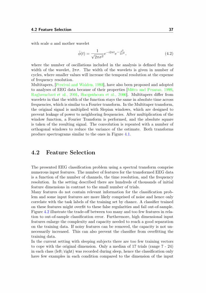
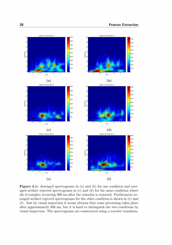
Figure 4.1: Averaged spectrograms in (a) and (b) for one condition and aver-aged artifact rejected spectrograms in (c) and (d) for the same condition wherethe k-complex occurring 300 ms after the stimulus is removed. Furthermore av-eraged artifact rejected spectrograms for the other condition is shown in (e) and(f). Just by visual inspection it seems obvious that some processing takes placeafter approximately 800 ms, but it is hard to distinguish the two conditions byvisual inspection. The spectrograms are constructed using a wavelet transform.

4.2 Feature Selection 39
space. One way to obtain more examples is to use the trials across subjects,but it has been shown in BCI settings that "good" features usually cannot betransferred from one person to another without problems. Brain structures arenot organized exactly the same way, and hence brain signal characteristics varybetween subjects, and some subjects even lack typical mu-rhythm activity, seee.g. [Lal et al., 2004, Pfurtscheller and Lopes da Silva, 1999]. Furthermore, therecording positions can not be controlled in enough detail to transfer directlysince the exact positioning of EEG caps is difficult and the re-application atdifferent recording sessions does not result in identical recording positions. Thismeans that an optimal set of features has to be determined for each subjectthough there might be some overlap.However, there are also obvious benefits in reducing the number of input fea-tures. The interpretability of the recorded signal is improved by extractinga few significant features. For new experimental paradigms, prior knowledgeabout the importance of features is limited and might even be misleading iftransferred directly from other paradigms.Selecting a subset of features can also lead to improved experiments. If only asubset of channels proves to be relevant future, EEG research can e.g. rely ona reduced set of electrodes.
4.2.1 NIPS 2003 Feature Selection Challenge Summary
One of the most rigorous investigations of different feature selection schemes isthe NIPS 2003 Feature Selection Challenge [Guyon et al., 2004]. This is the maininspiration for the selected methods in this thesis. To summarize the results ofthe NIPS 2003 Feature Selection Challenge [Guyon et al., 2006] it is found thatnon-linear classifiers generally outperform linear classifiers in the competition.Even for data sets with a high number of features and few examples adequateregularization of nonlinear classifiers leads to better performance than linearclassifiers. The SVM is furthermore identified as a versatile classifier.7 out of 10 of the best performing classifiers use some feature selection strategywhere most used forward selection or backward elimination inspired approaches.Forward selection algorithms starts with an empty set of features and then pro-gressively add features based on some measure of improvement of performance.The backward elimination algorithms starts with a full set of unranked featuresand then progressively removes the least important features. Though some ofthe top entrants use embedded methods, others perform well using all the avail-able features. Unsupervised dimensionality reductions methods, e.g. PrincipalComponent Analysis, PCA, are shown to work well, as are filter methods likethe Pearson correlation coefficient.

40 Feature ExtractionC
lass
ifica
tion
Err
or
# ranked features included
Meaningful, not redundant Meaningful, redundant
Noisy
Figure 4.2: The figure shows a typical behavior of the classification errorversus the size of the selected feature subset for a setting where the features areranked according to their relevance to the classification task. (Adapted from[Tangermann, 2007])
4.2.2 Univariate Methods
To test the relevance of individual features simple univariate methods, suchas the T-test, F-score etc., can be employed, and they usually perform quitewell [Guyon et al., 2006]. A univariate ranking index for a binary classificationproblem use a test statistic to compare means or variances of two assumedgaussian processes. The T-statistic compares the means of two classes and therealization, t, of the statistic T is given by
t =µA − µB
(mA−1)s2A+(mb−1)s2BmA+mB−2
√1mA
+ 1mB
, (4.3)
where mA and mB are the number of trials in each class, µA and µB are themeans of each class, and sA and sB are the estimated standard deviation, [Guyonet al., 2006]. The absolute value of the T-statistic can be used directly as aranking criterion, with the largest value corresponding to the most informativefeature. Feature ranking based on such a correlation makes an implicit orthog-onality assumption and do not take mutual information between features into

4.2 Feature Selection 41
account. However, this assumption is rarely valid, especially not in high di-mensional settings such as the presented EEG classification, where features arehighly correlated.
4.2.3 Multivariate Embedded Methods
Multivariate embedded methods deal with the shortcomings of univariate meth-ods. The term embedded refers to the relation between the feature selectionmethod and the classification method. Embedded methods integrate the classi-fication algorithm in the feature selection algorithm and this coupling leads to agood feature subset while the classifier is trained. Among the embedded meth-ods used for feature selection, the greedy algorithms based on forward selectionand backward elimination are the most popular. A popular embedded methodis a backward elimination algorithm proposed by [Guyon et al., 2002]. The Re-cursive Feature Elimination, RFE, algorithm operates by trying to choose thesubset of features, which leads to the largest margin of class separation using ameasure given by the SVM classifier itself. The algorithm is mostly used withlinear SVMs where the weights directly apply as a measure, but it can be gen-eralized to the non-linear case. In the present thesis the non-linear version isused in a modified version. In the case of a linear SVM, the decision function isgiven by f(x) = wx+ b, and the algorithm iteratively removes the feature withthe smallest weight, |wi|, and retrains the model until all features are ranked.In the non-linear case it iteratively removes the features leading to the smallestchange in the SVM cost function, see Equation (3.29). Hence the RFE is apruning method according to the smallest change in objective function. At theexpense of sub-optimality, several features can be removed at every iteration.For high dimensional data it is common practice, see e.g. [Guyon et al., 2006],to remove chunks of the features at every iteration. The algorithm is describedin Algorithm 1. Compared to the original algorithm, it is modified such thatthe σ and C parameter is re-estimated for every reduced subset of features, thissimple improves the performance. Furthermore the full cost function is esti-mated using a modified output of LIBSVM since it normally does not returnthis value.In the present implementation, see Algorithm 1, the number of features that areremoved in every iteration of the algorithm is adjusted depending on the remain-ing number of features. Hence, during the first few iterations, large chunks offeatures are removed, whereas later in the process only few features are removedevery iteration. This will be further discussed in Section 5.5.3. To select theoptimal number of features, [Guyon et al., 2002] simply evaluate the accuracydirectly on the test set for different sized subsets of genes in a gene selectiontask. Alternatively it could be based on the ranking criterion itself or by split-ting the training set into two new sets, where one is used for validation and on

42 Feature Extraction
for training, and then pick the optimal number of features based on the predic-tive performance on the validation set. This procedure however, proves to berather intractable and results in this thesis are therefore presented inspired by[Guyon et al., 2002].The algorithm, see Algorithm 1, is implemented in Matlab and it turns out thatit can benefit from the result in Section 3.6.3 and 5.5.2. During evaluation of thesingle features, the stopping tolerance can be adjusted to reduce computationaltime. To obtain the the margin based ranking criterion, LIBSVM [Chang andLin, 2011] is modified to produce the desired values.

4.2 Feature Selection 43
Algorithm 1 Modified Recursive Feature EliminationInput:Training examplesX0 = [x1;x2; . . . ;xl]Class labelsY0 = [y1; y2; . . . ; yl]
Initilalize:Feature subset of all original featuress = [1, 2, ..., n]Empty subset of ranked featuresr = [ ]
while s non-empty doReduce training examples to surviving feature indicesX = X0(:, s)
Estimate SVM parameters for the reduced set of features(σ,C) = crossval(X,T0)
Train the SVM classifier on the feature subspace defined by sW = svmtrain(Y0,X) ( i.e. W = (αT − 1
2αT yiyjK(xi, xj)α))
For each feature m ∈ s compute the ranking scorefor m = 1→ size(s) do
W\m = svmtrain(Y0,X\m)end forC(i) = abs(W2 −W\m
2)
Find the feature with the smallest ranking criterionf = argmin(C(i))
Update indicesr = [s(f), r]s=s(1:f-1,f+1:length(s))
%%% Modification to remove P % of the features at every iterationFind least important features[∼, f] = sort(C, 1, ’ascend’);Update the ranked feature listr = [fliplr(s(f(1 : ceil(size(X, 2)/P )))), r];Remove the least important featuress(f(1 : ceil(size(X, 2)/P ))) = [ ];%%%
end whileOutput:Ranked list of features r

44 Feature Extraction

Chapter 5
Model Selection
As mentioned earlier, the amount of examples available for training a single-subject classifier is rather limited since only a median of 17 examples (range 7- 24) are available in each class (left/right). Therefore a resampling strategy isapplied to obtain robust estimates of the performance of the classification al-gorithm. In doing this, the possibility of estimating sound bounds on the errordiminishes, but for high-dimensional data sets with few examples this is gen-erally not possible anyway, see [Guyon et al., 1998]. In the following a generaldescription of high dimensional spaces in low sample size settings is given as thisis the condition of the used data set. Then a cross-validation approach appli-cable to this is described, along with a way to test significance of the obtainedresults. Some small synthetic data sets are introduced to illustrate various as-pects of parameter selection. Finally, measures to evaluate the performance areintroduced.
5.1 The Curse of Dimensionality
The term "curse of dimensionality" is commonly used to describe challengesin high dimensional spaces, [Bishop, 2007]. Especially geometrical intuitionsfrom two and three dimensions are not always valid in high dimensional spaces.[Hall et al., 2005] investigate general properties of high dimensional low sample
46 Model Selection
size data in a classification setting and present some rather interesting insights.They prove for a finite sample size setting that all points will lose subsequentlymore of their spatial topology if dimensionality is increased towards infinity. Inthe presented asymptotic case of infinity, the points will be pairwise orthogonal.Furthermore, they will be asymptotically located on the vertices of a regularsimplex where all points have almost the same distances to the origin as well asamong each other.This distance concentration, where all distances in high dimensional space arealmost equal, is just one aspect of the special characteristics posed by high di-mensional problems. Low sample size high dimensional data additionally givesrise to the phenomenon known as hubness, see [Radovanović et al., 2010]. Thisphenomenon is related to the number of times a point occurs among the k nearestgeometric neighbors. It is shown for a wide range of problems, see [Radovanovićet al., 2010], that when dimensionality is increased, the distribution of the num-ber of occurrences becomes considerably skewed. Few points appear to be thenearest geometric neighbor to other points more often. Nevertheless, the phe-nomena of hubs is related to the distance concentration. As shown by [Hallet al., 2005], the points in low sample size high dimensional settings are almostorthogonal with the same distance to each other and to the origin of the high di-mensional simplex. If one point is an "outlier" in the sense that it is a little closerto the the simplex origin than the rest are, it is then also closer to several otherpoints. Hence hubs are outliers in the sense that they are found in low densityareas of the distribution, but are close to many other points. Normally outliersare thought of as further away from the center, this is not the case for hubs.These observations can influence classifier performance if not handled with care.
5.2 Cross-validation
A common approach, to avoid overfitting due to the resampling, is to use cross-validation. This is a technique where subsets of data are held out and usedfor validation, while the model is trained on the remaining data [Bishop, 2007].This procedure is repeated and the quality of the predictions across the test setsare averaged to yield an overall measure of the predictive power, i.e. the testerror. The mean accuracy of the single SVM estimated on the hold-out set isan unbiased estimator of the mean. Furthermore, in a resampling setting, themean of several unbiased estimates also produces a new unbiased estimate ofthe mean. The exact strategy for determining the size of the training- and test-subset may vary. One form of cross-validation leaves out a single observationat a time, whereas K-fold cross-validation splits the data into K subsets, whichare each used for validation. Both the kernel- and the regularization parameter

5.3 Permutation Test 47
are chosen using this strategy within the training set.In a two class classification task it is common practice to use a leave-two-outprocedure, where one example from each class is left out of the training set. Inthe presented data set the leave-two-out procedure is applied on balanced datasets, i.e. a number of trials are left completely out at every iteration to obtain anequal number of examples in each class. This is done to avoid that the trainedclassifier just behaves as "majority" classifier. In continuation of the generalproperties presented for high dimensional spaces, [Hall et al., 2005] show that abasic SVM will predict based on the majority class alone for a dimension towardsinfinity if the inter-distance between two classes is too small. Furthermore, forunbalanced data, it is shown that the SVM gives asymptotically completely in-correct classification for the population with the smaller sample. Inspired bythese results [Klement et al., 2008] show that infinity is not that large in prac-tice, especially not for the soft margin SVM. This means that a leave-one-outprocedure will misclassify all examples even for rather low dimensional data ifonly a small number of examples are available for training.
5.3 Permutation Test
While the mean of the errors obtained via cross-validation is indeed an unbiasedestimate of the expected error, the variance is not. The cross-validation trialsare not independent and hence it requires thorough modeling of the dependenceto avoid a too optimistic estimate of the variance. An alternative is to use apermutation test to estimate how likely it is to obtain the result by chance,due to some random pattern detected by the SVM in the high dimensional data[Golland and Fischl, 2003, Golland et al., 2005, Efron and Tibshirani, 1993]. Theresult provided by the permutation test provides a weaker answer than standardconvergence bounds, since it gives no indication of how well the obtained errorrate will generalize. However, it does answer whether the classification resultcould be obtained by chance.The null hypothesis of the permutation test is that the SVM cannot learn topredict labels based on the given training set and works under the assumptionthat the data distribution is adequately represented by the sample data.For a set of examples, xi, yimi=1, with all the possible permutations, Zm forindices 1...m, and with the test statistic T based on the cross-validation error,the permutation test procedure consists of N iterations, see Algorithm 2.Ideally the full set of permutations should be used to generate the cumulativedistribution, P , but this is not computational tractable, and hence the algorithmrelies on sampling from Zm. This strategy is feasible as long as N is sufficientlylarge.
48 Model Selection
Algorithm 2 Permutation Testfor n = 1→ N do
Sample a permutaion zn = (zn1 , ..., znm) from a uniform distribution over
Zm
Compute the statistic tn = T (x1, yzn1 , ...,xm, yznm)end for
Construct an empirical cumulative distribution
P (T ≤ t) =1
N
N∑n=1
Θ(t− tm)
where Θ is a step function (Θ(x) = 1, ifx > 0; 0 o.w.)
Compute the statistic for the true labels, t0 = T (x, y, ...,xm, ym) and thecorresponding p-value p0 under the empirical distribution P
Reject the null hypothesis if p0 ≤ α, where α is the acceptable significancelevel
5.4 Synthetic Data
In addition to the main analysis of the presented EEG data some synthetic datasets are created to investigate the performance of the classifier and to illustratee.g. kernel behavior.The Exclusive OR, XOR, problem is a classical problem used to illustrate chal-lenges in classification problems. Examples of the XOR problem is the chess-board problem seen in Figure 5.4 and the intertwined circles seen in Figure 5.1.It is clear that neither the input variable x1 nor x2 is able to perform the classi-fication independently whereas patterns or regularities in the data can be foundif the combination of x1 and x2 is used. If the input data is composed of addi-tional noisy features the shown regularity might not be found through classicalstatistical analysis. In that case more advanced methods can be employed toretrieve the two relevant features thus also simplifying the classification task.Furthermore the chessboard like patterns require highly non-linear decisionboundaries, and hence is a good problem to test non-linear classifiers on.Likewise, the problem composed of two intertwined semi-circles, see Figure 5.1,is a good XOR problem for illustrating kernel properties.Finally two high dimensional problems are constructed. An XOR data set with
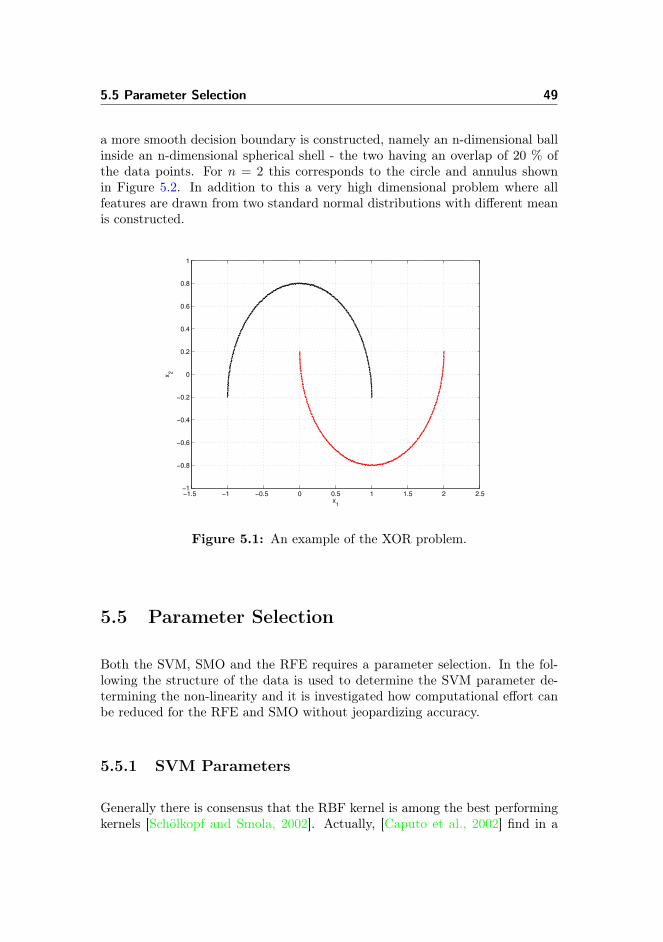
5.5 Parameter Selection 49
a more smooth decision boundary is constructed, namely an n-dimensional ballinside an n-dimensional spherical shell - the two having an overlap of 20 % ofthe data points. For n = 2 this corresponds to the circle and annulus shownin Figure 5.2. In addition to this a very high dimensional problem where allfeatures are drawn from two standard normal distributions with different meanis constructed.
−1.5 −1 −0.5 0 0.5 1 1.5 2 2.5−1
−0.8
−0.6
−0.4
−0.2
0
0.2
0.4
0.6
0.8
1
x1
x2
Figure 5.1: An example of the XOR problem.
5.5 Parameter Selection
Both the SVM, SMO and the RFE requires a parameter selection. In the fol-lowing the structure of the data is used to determine the SVM parameter de-termining the non-linearity and it is investigated how computational effort canbe reduced for the RFE and SMO without jeopardizing accuracy.
5.5.1 SVM Parameters
Generally there is consensus that the RBF kernel is among the best performingkernels [Schölkopf and Smola, 2002]. Actually, [Caputo et al., 2002] find in a
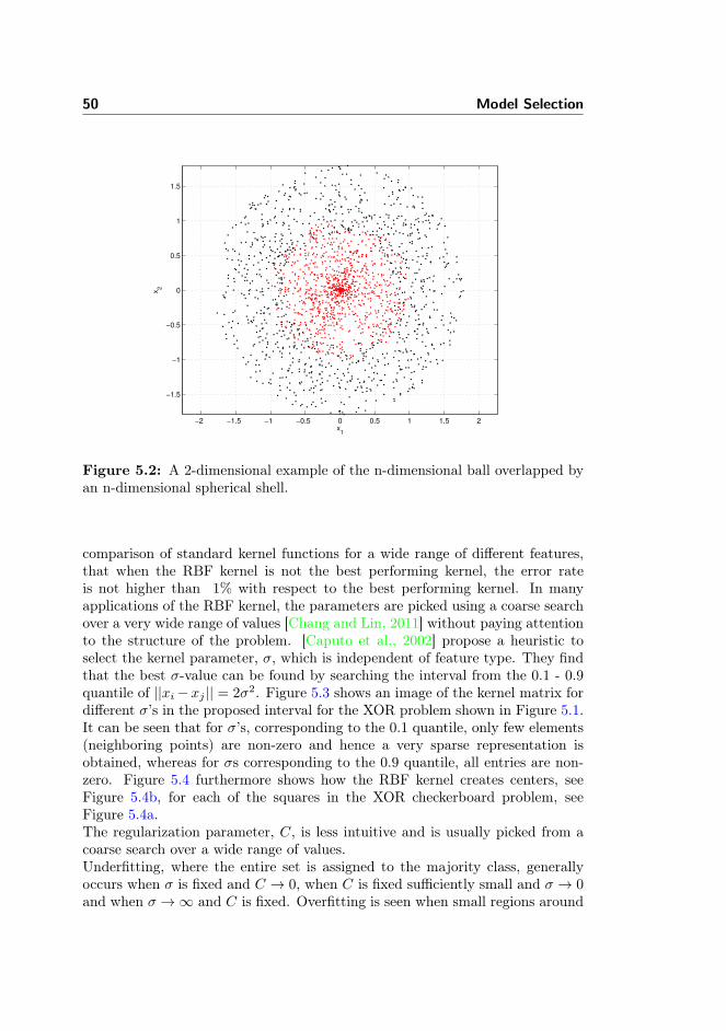
50 Model Selection
−2 −1.5 −1 −0.5 0 0.5 1 1.5 2
−1.5
−1
−0.5
0
0.5
1
1.5
x1
x2
Figure 5.2: A 2-dimensional example of the n-dimensional ball overlapped byan n-dimensional spherical shell.
comparison of standard kernel functions for a wide range of different features,that when the RBF kernel is not the best performing kernel, the error rateis not higher than 1% with respect to the best performing kernel. In manyapplications of the RBF kernel, the parameters are picked using a coarse searchover a very wide range of values [Chang and Lin, 2011] without paying attentionto the structure of the problem. [Caputo et al., 2002] propose a heuristic toselect the kernel parameter, σ, which is independent of feature type. They findthat the best σ-value can be found by searching the interval from the 0.1 - 0.9quantile of ||xi−xj || = 2σ2. Figure 5.3 shows an image of the kernel matrix fordifferent σ’s in the proposed interval for the XOR problem shown in Figure 5.1.It can be seen that for σ’s, corresponding to the 0.1 quantile, only few elements(neighboring points) are non-zero and hence a very sparse representation isobtained, whereas for σs corresponding to the 0.9 quantile, all entries are non-zero. Figure 5.4 furthermore shows how the RBF kernel creates centers, seeFigure 5.4b, for each of the squares in the XOR checkerboard problem, seeFigure 5.4a.The regularization parameter, C, is less intuitive and is usually picked from acoarse search over a wide range of values.Underfitting, where the entire set is assigned to the majority class, generallyoccurs when σ is fixed and C → 0, when C is fixed sufficiently small and σ → 0and when σ →∞ and C is fixed. Overfitting is seen when small regions around

5.5 Parameter Selection 51
the training examples of the smallest class are classified to be that class, whilethe rest is classified as the majority class. This occurs in the case where σ → 0and C is sufficiently large and when σ is fixed and C →∞ for noisy data sincethe SVM classifier strictly separates the training examples of the two classes.The linear kernel matrix is shown in Figure 5.3d. Though there is little visualresemblance between the images, it can be shown that for σ → ∞ and properscaling of C the non-linear SVM classifier with RBF kernel converges to thelinear SVM classifier, [Keerthi and Lin, 2003].
Theorem 5.1 For a proper fixed value of C = Cσ2 and σ →∞ the non-linearSVM with a Gaussian RBF kernel converges to the linear SVM.
Proof. For σ →∞ the Gaussian RBF kernel function can be written, using aseries expansion, as
K(x, x) = exp
(−‖x− x‖
2
2σ2
)(5.1)
=1− ‖x− x‖2
2σ2+O
(‖x− x‖2
σ2
)(5.2)
=1− ‖x‖2
2σ2− ‖x‖
2
2σ2− xTx
σ2+O
(‖x− x‖2
σ2
). (5.3)
Using this approximation, the quadratic term of the objective function 3.29 inthe non-linear version of the SVM can be written as∑
i
∑j
αiαjyiyjK(x, x) =
∑i
∑j
αiαjyiyj
−∑i
∑j αiαjyiyj‖xi‖2
2σ2
−∑i
∑j αiαjyiyj‖xj‖2
2σ2
+
∑i
∑j αiαjyiyjx
Ti xj
σ2
+12
∑i
∑j αiαjyiyj∆ij
σ2, (5.4)
where limσ2→∞
∆ij = 0.
By defining αi = αiσ2 and using the constraint from the QP-formulation in (3.29)
(∑mi=1 αiyi = 0) in the three first terms of the approximation in (5.4), the
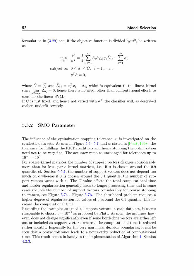
52 Model Selection
formulation in (3.29) can, if the objective function is divided by σ2, be writtenas
minα
F
σ2=
1
2
m∑i,j=1
αiαjyiyjKij −m∑i=1
αi
subject to: 0 ≤ αi ≤ C, i = 1, ...,m
yT α = 0,
where C = Cσ2 and Kij = xTi xj + ∆ij which is equivalent to the linear kernel
since limσ2→∞
∆ij = 0, hence there is no need, other than computational effort, to
consider the linear SVM.If C is just fixed, and hence not varied with σ2, the classifier will, as describedearlier, underfit severely.
5.5.2 SMO Parameter
The influence of the optimization stopping tolerance, ε, is investigated on thesynthetic data sets. As seen in Figure 5.5 - 5.7, and as stated in [Platt, 1998], thetolerance for fulfilling the KKT conditions and hence stopping the optimizationneed not to be very fine. The accuracy remains unchanged for tolerances up to10−1 − 100.For sparse kernel matrices the number of support vectors changes considerablymore than for less sparse kernel matrices, i.e. if σ is chosen around the 0.9quantile, cf. Section 5.5.1, the number of support vectors does not depend toomuch on ε whereas if σ is chosen around the 0.1 quantile, the number of sup-port vectors varies with ε. The C value affects the total computational timeand harder regularization generally leads to longer processing time and in somecases reduces the number of support vectors considerably for coarse stoppingtolerances, see Figure 5.7a - Figure 5.7b. The chessboard problem requires ahigher degree of regularization for values of σ around the 0.9 quantile, this in-crease the computational time.Regarding the examples assigned as support vectors in each data set, it seemsreasonable to choose ε = 10−3 as proposed by Platt. As seen, the accuracy how-ever, does not change significantly even if some borderline vectors are either leftout or included as support vectors, whereas the computational time is reducedrather notably. Especially for the very non-linear decision boundaries, it can beseen that a coarse tolerance leads to a noteworthy reduction of computationaltime. This result comes in handy in the implementation of Algorithm 1, Section4.2.3.
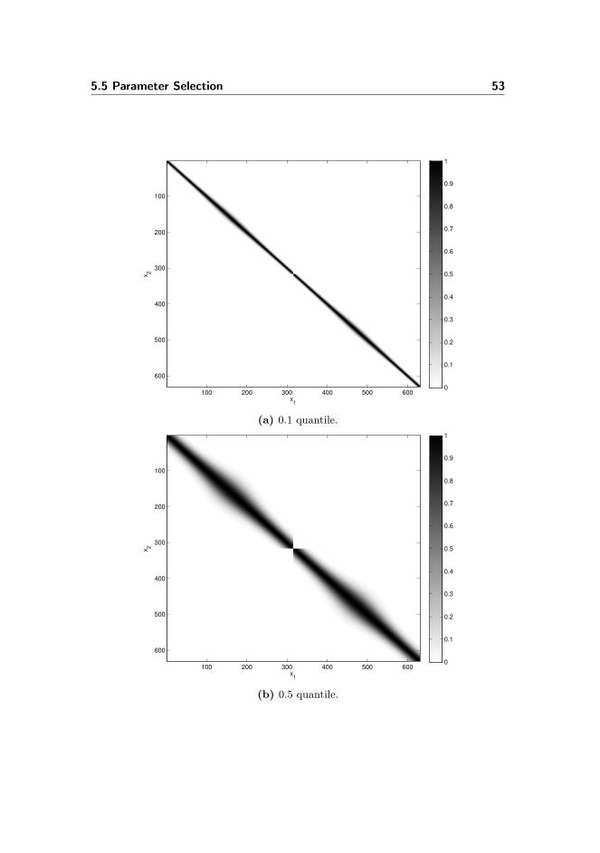
5.5 Parameter Selection 53
x1
x2
100 200 300 400 500 600
100
200
300
400
500
600
0
0.1
0.2
0.3
0.4
0.5
0.6
0.7
0.8
0.9
1
(a) 0.1 quantile.
x1
x2
100 200 300 400 500 600
100
200
300
400
500
600
0
0.1
0.2
0.3
0.4
0.5
0.6
0.7
0.8
0.9
1
(b) 0.5 quantile.
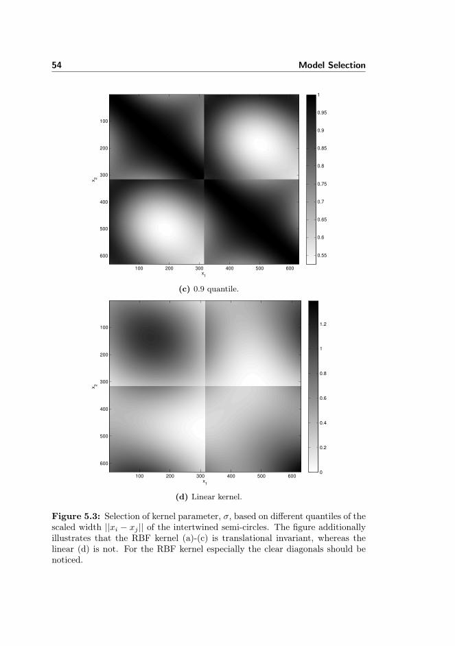
54 Model Selection
x1
x2
100 200 300 400 500 600
100
200
300
400
500
600 0.55
0.6
0.65
0.7
0.75
0.8
0.85
0.9
0.95
1
(c) 0.9 quantile.
x1
x2
100 200 300 400 500 600
100
200
300
400
500
600
0
0.2
0.4
0.6
0.8
1
1.2
(d) Linear kernel.
Figure 5.3: Selection of kernel parameter, σ, based on different quantiles of thescaled width ||xi − xj || of the intertwined semi-circles. The figure additionallyillustrates that the RBF kernel (a)-(c) is translational invariant, whereas thelinear (d) is not. For the RBF kernel especially the clear diagonals should benoticed.

5.5 Parameter Selection 55
−1 −0.8 −0.6 −0.4 −0.2 0 0.2 0.4 0.6 0.8 1−1
−0.8
−0.6
−0.4
−0.2
0
0.2
0.4
0.6
0.8
1
x1
x2
(a) 2 x 2 chessboard XOR problem.
x1
x2
100 200 300 400 500 600 700 800
100
200
300
400
500
600
700
800 0
0.1
0.2
0.3
0.4
0.5
0.6
0.7
0.8
0.9
1
(b) Corresponding kernel for σ based on the 0.1 quantile.
Figure 5.4: The image of the kernel matrix for the 2 x 2 chessboard XORproblem shows how the RBF kernel creates a center for each ofthe squares.

56 Model Selection
10−5
10−4
10−3
10−2
10−1
100
50
55
60
65
70
75
80
85
90
95
100
Stopping Tolerance
%
time
accuracy
nSV
(a)
10−5
10−4
10−3
10−2
10−1
100
50
55
60
65
70
75
80
85
90
95
100
Stopping Tolerance
%
time
accuracy
nSV
(b)
Figure 5.5: 50-dimensional ball and spherical shell with 1,000 examples in eachclass for both the test and training set. In (a) σ is chosen as the 0.1 quantile andC = 102 and in (b) σ is chosen as the 0.9 quantile. The results are averaged over100 data sets. The two classes are overlapping, hence around 90% classificationaccuracy is expected.Time and nSV (number of support vectors) are divided bytheir maximum values.
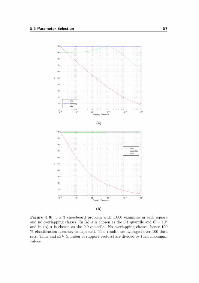
5.5 Parameter Selection 57
10−5
10−4
10−3
10−2
10−1
100
0
10
20
30
40
50
60
70
80
90
100
Stopping Tolerance
%
time
accuracy
nSV
(a)
10−5
10−4
10−3
10−2
10−1
100
0
10
20
30
40
50
60
70
80
90
100
Stopping Tolerance
%
time
accuracy
nSV
(b)
Figure 5.6: 3 x 3 chessboard problem with 1,000 examples in each squareand no overlapping classes. In (a) σ is chosen as the 0.1 quantile and C = 102
and in (b) σ is chosen as the 0.9 quantile. No overlapping classes, hence 100% classification accuracy is expected. The results are averaged over 100 datasets. Time and nSV (number of support vectors) are divided by their maximumvalues.

58 Model Selection
10−5
10−4
10−3
10−2
10−1
100
95.5
96
96.5
97
97.5
98
98.5
99
99.5
100
Stopping Tolerance
%
time
accuracy
nSV
(a)
10−5
10−4
10−3
10−2
10−1
100
0
10
20
30
40
50
60
70
80
90
100
Stopping Tolerance
%
time
accuracy
nSV
(b)
Figure 5.7: 10,000 dimensional examples with all features drawn from normaldistributions. One class has mean +1 for all features, the other class has mean-1 for all features. σ is chosen as the 0.9 quantile and C = 1 and C = 108 in(a) and (b) respectively. The results are averaged over 10 data sets. Time andnSV (number of support vectors) are divided by their maximum values. In (a)both nSV and accuracy is 100 and in (b) accuracy is 100.
5.6 Evaluation of Model Performance 59
5.5.3 RFE Parameters
The implementation of the RFE algorithm described in Section 4.2.3 removes25 % of the features during each iteration while the feature dimension is over1,000, and removes 10 % during each iteration when a feature dimension below1,000 is obtained. This approach gives very comparable results to just removing5 % of the features during all iterations, but reduces the time considerably.The SVM parameters are re-estimated during every iteration as this improvesresults significantly. Especially re-estimating the σ-parameter is important asthe problem changes size dramatically during the iterations. However, to reducecomputational time, only a very coarse grid is used to find values for C and σ.In the final implementation C is found searching a log2 interval and σ is foundusing a coarse grid from the 0.1 - 0.9 quantile of ||xi − xj || = 2σ2. Using a veryfine grid gives comparable performance for all subjects. The most importantparameter of the two proves to be σ and since a rather "narrow" feasible rangeis given from the inter- and intra class distance, this result is not surprising.Furthermore a value of ε = 10−2 is used as stopping criterion in the RFE algo-rithm. When evaluating final performance ε = 10−3 is used.
5.6 Evaluation of Model Performance
The SVM classifier is evaluated in terms of achieved prediction error (one minusthe number of correct predictions divided by the total number of predictions).Additionally the permutation test is conducted corresponding to a 95% signif-icance level. In addition to the permutation test described in Section 5.3 theclassifier is also evaluated on the data presented in the awake condition and ondata obtained solely over the visual cortex (electrodes O1 and O2). The datafrom the awake condition is expected to contain enough information for an ac-tual classification in most cases and the data obtained over the visual cortex isexpected to show less or no predictive power.

60 Model Selection

Chapter 6
Results
The following chapter analyses the EEG data obtained from the experimentdescribed in Section 2.3. The EEG data is pre-processed as described in thenext section and then analyzed using the setup described in the previous chap-ters. The SVM described in Chapter 3 is combined with the two feature se-lection schemes described in Chapter 4. All parameters are tuned as describedin Section 5.5. Performance is assessed using the balanced leave-two-out cross-validation scheme described in Section 5.2 and significance is evaluated usingthe permutation test described in Section 5.3. Everything is implemented inMatlab. The results are reported in this chapter and discussed in the followingchapter.
A general overview of the subjects included in the analysis is shown in Ta-ble 6. The table shows the number of trials obtained during wakefulness andduring sleep. As can be seen, the number of trials included for the differentsubjects to obtain a balanced training and test set varies between 14 and 46.
6.1 Data Pre-processing
The raw EEG data are pre-processed using a Matlab toolbox developed by SidKouider, École Normale Supérieure, Leonardo da Silva Barbosa, École Normale

62 Results
Subject Sleep Sleep Balanced Awake Awake BalancedEL ER no. of trials L R no. of trials
105 20 22 40 21 15 30107 17 16 32 20 22 40109 16 20 32 22 24 44111 17 7 14 16 20 32113 20 17 34 21 21 42117 9 13 18 12 13 24118 20 17 34 24 24 48122 17 16 32 15 15 30127 18 17 34 22 21 42129 10 10 20 18 19 36134 21 24 42 18 21 36137 21 19 38 15 16 30138 10 9 18 18 19 36139 10 17 20 21 25 42144 16 19 32 15 13 26147 21 22 42 15 15 30149 23 20 40 23 24 46150 23 24 46 23 20 40
Table 6.1: Overview of subjects and corresponding number of trials. EL,expected left, and ER, expected right, corresponds to the L, left, and R, rightin the awake case and indicates whether the expected response for the subjectis left or right (object vs. animal).
Supérieure, and Carsten Stahlhut, Technical University of Denmark. The tool-box is mainly based on other open source toolboxes for Matlab, namely SPM8[Ashburner et al., 2008], FieldTrip [Oostenveld et al., 2011] and EEGLAB [De-lorme and Makeig, 2004].The pre-processing steps include high-pass filtering, low-pass filtering, epoching,baseline correction and downsampling of the raw data.In addition to this all features are standardized, as recommended when dealingwith SVMs [Chang and Lin, 2011].The spectral transforms are found using the SPM8 interface to FieldTrip.Along with the general pre-processing, a more sparse representation of the EEGdata is found. This representation is more computational tractable and improvesthe predictive power of the classifier.

6.1 Data Pre-processing 63
6.1.1 Data Set Dimensionality Reduction
A spectral transform of the EEG data leads to a very high feature dimension.The dimension is a function of the number of channels × the frequency resolu-tion × the time resolution. For a standard wavelet transform of the 64 channelsignal with a frequency resolution of 1 Hz, this leads to a feature space with adimension greater than 106 for each trail.It is of course a trade off between tractability and information resolution whenthe dimensionality is reduced. However, it proves that reducing the spatiotem-poral resolution, i.e. binning frequencies into coarser intervals and reducing thetime resolution, not only leads to a reduction in computational time but alsoimproves the predictive power of the SVM. This is not surprising both from aphysical and data dimension point of view. Since only a few trials in each con-dition are present, the physiological variability between trials will lead to toomuch difference between relevant features. If the time and frequency resolutionis too fine and only a few features can be selected by the feature selection algo-rithm to reduce noise, there will simply not be an overlap of features betweenthe different trials. Additionally, when the resolution is reduced, the power ofinformative features will increase. On the other hand if the resolution is re-duced too much, the informative features will lose information due to too much"averaging" with the neighboring features. As proposed by e.g. [Pfurtschelleret al., 2006], the most important electrodes are in the motor cortex area aroundC3 and C4, hence a considerable sparse prior to apply, is that only those twoelectrodes are included in the analysis. The predominant frequencies are ex-pected to lie in the interval 4-40 Hz as described in Section 2.2, and hence thefrequency interval from 4 - 40 Hz is used with steps of 4 Hz. The original timeresolution is reduced to 50 Hz. This gives a more manageable dimension of thefeature space, namely 2,800.One (sub)optimal configuration is to use a 7 cycle wavelet transform with fre-quency intervals of 4 Hz in the range 4 - 40 Hz and a reduce the number of timesamples, using the subsample option = 10. If nothing else stated, results areobtained using this representation, which is denoted the reduced data set in thefollowing.
6.1.2 Artifact Rejection
An artifact rejected data set is constructed to investigate possible improvements,see Figure 4.1. The artifacts found in EEG data sets recorded during sleep aresignificantly different from the ones found in a normal EEG signal. Especiallysome auditory components and K-complexes have been removed in the artifact
64 Results
rejected data set using Independent Component Analysis, ICA. In the awakecondition as well as during sleep, auditory components were removed from vir-tually all trials, whereas the K-complexes are only present during sleep. Onlyduring wakefulness eye movements are removed, since these disappear duringearly sleep phases.
6.2 Feature Selection
Both the reduced data set described in 6.1.1 and the full wavelet transform leadsto classification accuracies for all subjects around 50 % if no feature selection isperformed. Hence the results are not described in further detail. In the followingthese results obtained using feature selection are presented.
6.3 T-Test Based Feature Selection
Using the T-test described in Section 4.2.2 generally leads to a poor classifierperformance around chance level for the full spectral transform. On the reduceddata set, the picture changes and it is possible to obtain significant results for atleast 11 subjects though in general performance is worse or at best comparable tousing the RFE approach, hence the results are not described in further detail.A comparison of the two methods can be seen in Figure 6.1. It shows theobtained error rates averaged over all 18 subjects. A major advantage of thet-test based feature selection is that the computational burden is significantlyreduced compared to the RFE. This feature selection approach also leads to anti-learning, which is classification performance consistently worse than chance, ina few subjects, see discussion in Section 7.2 for further details.
6.4 RFE Feature Selection
Using the RFE based features selection requires more computational effort butleads to compelling performance. Results for all subjects are presented in Figure6.3 - 6.6 and in Appendix A. For a majority of the subjects classification bet-ter than chance is possible. The corresponding features selected to obtain thereported results are harder to interpret. There is no single conclusion readilyavailable, but classification performance combined with inspection of the featureselection yields several insights to extract. For each subject a figure showing
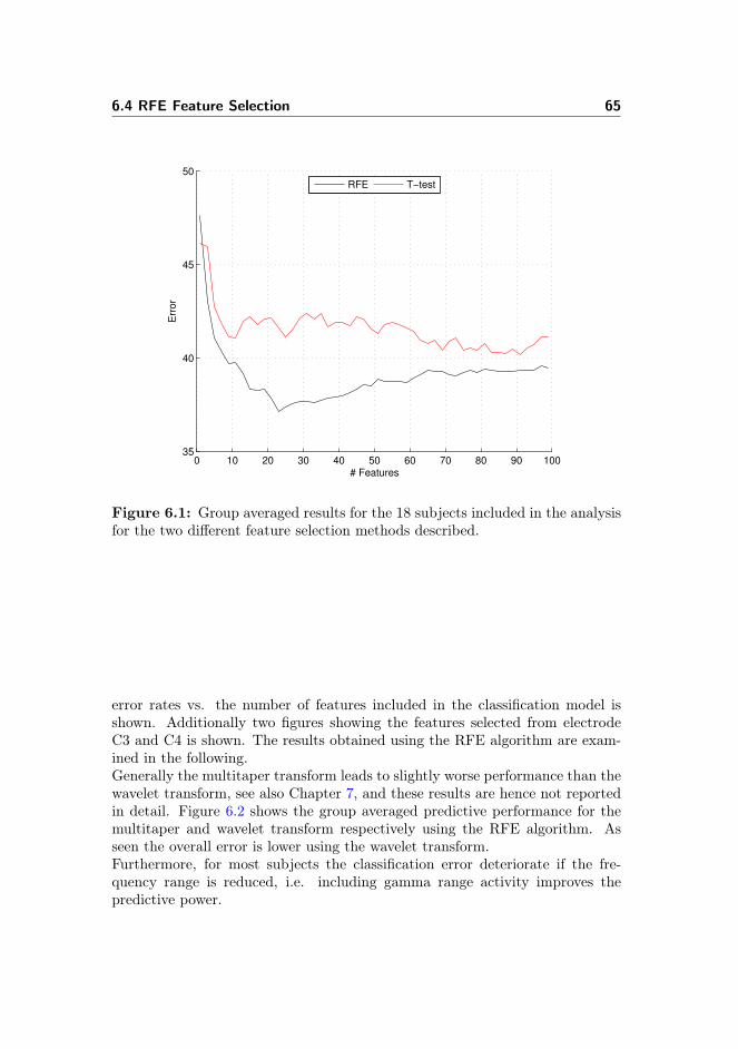
6.4 RFE Feature Selection 65
0 10 20 30 40 50 60 70 80 90 10035
40
45
50
# Features
Err
or
RFE T−test
Figure 6.1: Group averaged results for the 18 subjects included in the analysisfor the two different feature selection methods described.
error rates vs. the number of features included in the classification model isshown. Additionally two figures showing the features selected from electrodeC3 and C4 is shown. The results obtained using the RFE algorithm are exam-ined in the following.Generally the multitaper transform leads to slightly worse performance than thewavelet transform, see also Chapter 7, and these results are hence not reportedin detail. Figure 6.2 shows the group averaged predictive performance for themultitaper and wavelet transform respectively using the RFE algorithm. Asseen the overall error is lower using the wavelet transform.Furthermore, for most subjects the classification error deteriorate if the fre-quency range is reduced, i.e. including gamma range activity improves thepredictive power.
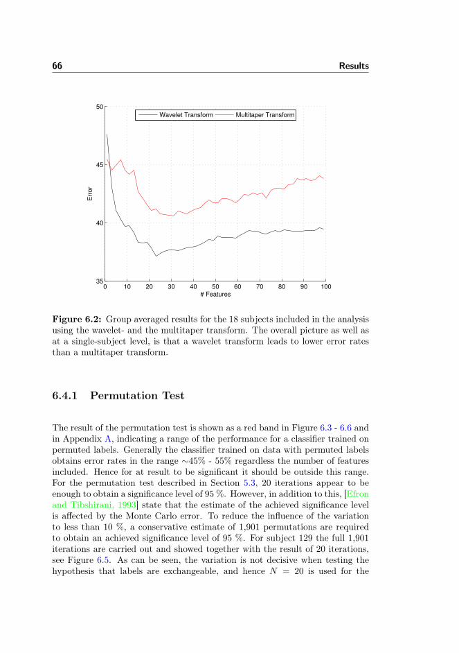
66 Results
0 10 20 30 40 50 60 70 80 90 10035
40
45
50
# Features
Err
or
Wavelet Transform Multitaper Transform
Figure 6.2: Group averaged results for the 18 subjects included in the analysisusing the wavelet- and the multitaper transform. The overall picture as well asat a single-subject level, is that a wavelet transform leads to lower error ratesthan a multitaper transform.
6.4.1 Permutation Test
The result of the permutation test is shown as a red band in Figure 6.3 - 6.6 andin Appendix A, indicating a range of the performance for a classifier trained onpermuted labels. Generally the classifier trained on data with permuted labelsobtains error rates in the range ∼45% - 55% regardless the number of featuresincluded. Hence for at result to be significant it should be outside this range.For the permutation test described in Section 5.3, 20 iterations appear to beenough to obtain a significance level of 95 %. However, in addition to this, [Efronand Tibshirani, 1993] state that the estimate of the achieved significance levelis affected by the Monte Carlo error. To reduce the influence of the variationto less than 10 %, a conservative estimate of 1,901 permutations are requiredto obtain an achieved significance level of 95 %. For subject 129 the full 1,901iterations are carried out and showed together with the result of 20 iterations,see Figure 6.5. As can be seen, the variation is not decisive when testing thehypothesis that labels are exchangeable, and hence N = 20 is used for the
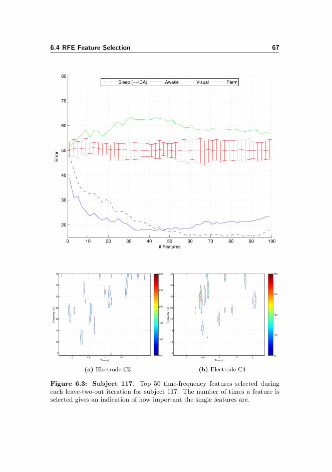
6.4 RFE Feature Selection 67
0 10 20 30 40 50 60 70 80 90 100
20
30
40
50
60
70
80
# Features
Err
or
Sleep (−−ICA) Awake Visual Perm
Time (s)
Fre
qu
en
cy (
Hz)
0 0.5 1 1.5 2
5
10
15
20
25
30
35
40
50
100
150
200
250
300
(a) Electrode C3
Time (s)
Fre
qu
en
cy (
Hz)
0 0.5 1 1.5 2
5
10
15
20
25
30
35
40
50
100
150
200
250
(b) Electrode C4
Figure 6.3: Subject 117. Top 50 time-frequency features selected duringeach leave-two-out iteration for subject 117. The number of times a feature isselected gives an indication of how important the single features are.
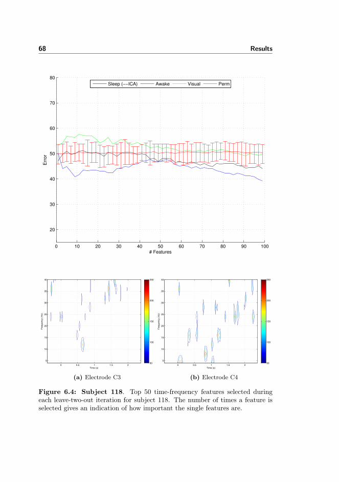
68 Results
0 10 20 30 40 50 60 70 80 90 100
20
30
40
50
60
70
80
# Features
Err
or
Sleep (−−ICA) Awake Visual Perm
Time (s)
Fre
qu
en
cy (
Hz)
0 0.5 1 1.5 2
5
10
15
20
25
30
35
40
50
100
150
200
250
(a) Electrode C3
Time (s)
Fre
qu
en
cy (
Hz)
0 0.5 1 1.5 2
5
10
15
20
25
30
35
40
50
100
150
200
250
(b) Electrode C4
Figure 6.4: Subject 118. Top 50 time-frequency features selected duringeach leave-two-out iteration for subject 118. The number of times a feature isselected gives an indication of how important the single features are.

6.4 RFE Feature Selection 69
0 10 20 30 40 50 60 70 80 90 100
20
30
40
50
60
70
80
# Features
Err
or
PermN=20
PermN=1901
Sleep Awake Visual
Time (s)
Fre
qu
en
cy (
Hz)
0 0.5 1 1.5 2
5
10
15
20
25
30
35
40
50
100
150
200
250
(a) Electrode C3
Time (s)
Fre
qu
en
cy (
Hz)
0 0.5 1 1.5 2
5
10
15
20
25
30
35
40
50
100
150
200
250
(b) Electrode C4
Figure 6.5: Subject 129. Top 50 time-frequency features selected duringeach leave-two-out iteration for subject 129. The number of times a feature isselected gives an indication of how important the single features are. In additionto the permutation test for N=20, the result of a test with N=1,901 is shown.

70 Results
0 10 20 30 40 50 60 70 80 90 100
20
30
40
50
60
70
80
# Features
Err
or
Sleep (−−ICA) Awake Visual Perm
Time (s)
Fre
qu
en
cy (
Hz)
0 0.5 1 1.5 2
5
10
15
20
25
30
35
40
50
100
150
200
250
(a) Electrode C3
Time (s)
Fre
qu
en
cy (
Hz)
0 0.5 1 1.5 2
5
10
15
20
25
30
35
40
50
100
150
200
250
(b) Electrode C4
Figure 6.6: Subject 139. Top 50 time-frequency features selected duringeach leave-two-out iteration for subject 139. The number of times a feature isselected gives an indication of how important the single features are.
6.4 RFE Feature Selection 71
remaining subjects.
6.4.2 Data From Pre-motor Cortex
Using data from electrodes C3 and C4 recorded during sleep, yields a classifierperformance significantly better than chance for 12 out of the 18 subjects, usingeither the artifact (subject 105, 113, 117, 134, 139, 144, and 150) or non-artifact(subject 107, 111, 122, 129, and 138) rejected data, see Figure 6.3 - 6.6 andFigure A.1 - A.14 in Appendix A. Some subjects get a much better signal,by removing artifacts, thus the artifact rejected data results are reported forthese subjects (labelled ICA). For others the manual artifact rejection does notchange the performance of the classifier. In some cases it removes to much ofthe signal, leading to worse classification performance. For these subjects, non-artifact rejected results are reported.Five subjects (subject 109, 118, 127, 137, and 147) are borderline cases regardingclassification performance, since only small parts of the feature subsets producesignificant classification results or classification error rates are close to chancelevel. In subject 149, see Figure A.13, anti learning behavior is seen. Thisbehavior is discussed in Section 7.2.Except for the cases where only few features are included in the model, thetraining error is generally 0 and most trials are treated as support vectors,though not all. Looking at classifier performance shows that a certain numberof features are needed to obtain the best classification, but including too manyfeatures leads to a decrease in performance, as depicted in Figure 4.2. Theplateau where including features neither improves nor worsen performance variesin size for the subjects. For subject 111 where a very low error rate is obtained,the plateau is around 100 features, which is not obvious from the shown plot,see Figure A.4. The best single-subject classification accuracy is exceeding 80%,see Figure 6.3, and several subjects yield accuracies around 70% - 80%. A fewsubjects, see e.g. Figure 6.4, have no or very little predictive signal. As statedearlier the accuracies are unbiased estimates, but it is not possible to obtainreliable error bars. However, those results not conflicting with the permutationinterval (red bars) are significant at a 95% level.
6.4.3 Data From Visual Cortex
Data recorded from electrodes O1/O2 during sleep is used as a proxy for visualcortex. It is expected that data collected from the visual cortex should notlead to good classification. However, it is not entirely the case, see Figure6.3 - 6.6 and Figure A.1 - A.14 in Appendix A. For subjects 137, see Figure

72 Results
A.9, and 149, see Figure A.13, the classifier yields results better than chancelevel. More puzzling are the results obtained for half of the subjects (107,111, 113, 117, 129, 134, 139, and 150). Here the classifier produces resultsworse than chance, implicating that flipping all labels would yield a classifierperforming significantly better than chance. Running a permutation test on thedata collected from O1/O2 yields chance level results as expected. The numberof predicted labels in each class are additionally relatively balanced, as are theerror rates for the two classes. This anti-learning behavior, where the classifierconsistently assign opposite class labels to the test set, indicates that thoughwith a special structure, signal is present in the data. This is discussed furtherin Section 7.2.
6.4.4 Data From the Awake Condition
Data collected from pre-motor cortex in the awake condition is also shown inFigure 6.3 - 6.6 and Figure A.1 - A.14 in Appendix A. Non-artifact rejected datayields a classifier performance better than chance for 7 out of the 18 subjects(109, 111, 117, 134, 138, 139, and 144) with up to 100 features included in themodel. One subject (118) is a borderline case. 6 subjects (107, 122, 127, 129,137, and 149) exhibit the anti-learning behavior further discussed in Section 7.2.However, several subjects indicate that including more features lead to betterclassification performance. This is investigated for all subjects including up toa 1,000 features. Additionally, the analysis is done on both artifact rejectedand non-artifact rejected data. In that case 10 of the 18 subjects yield goodclassification performance (109, 111, 113, 117, 118, 134, 138, 139, 144, and 149)where two of the subjects 111 and 113 gives the best performance on artifactrejected data. 6 subjects (107, 122, 127, 129, 137, and 147) show strong antileaning behavior where subject 122 and 147 gives the result for artifact rejecteddata. Only 2 out of the 18 subjects yield chance level results for the chosendata representation. The remaining 16 yield results different from chance. Onlyselected results are shown in Appendix C. For subject 113, see Figure C.1a, itcan be seen that building the model based on the top 200 features using artifactrejected data yields improved classifier performance and for subject 118, seeFigure C.1b, it can be seen that the model improves significantly by includingaround 250 features using non-artifact rejected data in the model.Very interestingly, it can be observed in general for all subjects, see Figure C.2aand C.2b for two examples, that anti-learning is reduced when more (noisy)features are added to the model. This behavior is similar to what is seen fornormal learning, see Figure 4.2. But conversely to learning, anti-learning isreversed to learning for some subjects, e.g. subject 149, see Figure C.2b, forthe non-artifact rejected data set. Here, if less than 100 features are included inthe training set, anti-learning is observed, whereas proper learning is observed

6.4 RFE Feature Selection 73
when more than 400 of the top ranked features are included in the training set.It is not always the case that anti-learning is reversed to learning by addingmore features. The representation might simply be too noisy compared to thenumber of available trials.
6.4.5 Spectro-histo-grams
Along with the obtained classification rates, the features selected to obtain theseare investigated. For every subject, see Figure 6.3 - 6.6 and Figure A.1 - A.14 inAppendix A, subfigures are shown corresponding to electrode C3 and electrodeC4. The figures are combined spectro- and histo- grams, showing the numberof times a feature is selected during the 300 iterations of the described cross-validation scheme, see Section 5.2. The histograms are composed by countingthe top 50 features. Acceptable inspection of the spectrograms and the corre-sponding selected features is a trade-off between noise and informative features.An increased number of features significantly increases the scattered noise andmakes it harder to see patterns, whereas decreasing the number of includedfeatures might remove too much information to actually see any patters. Thedominating patterns are present over a wider range of included features, butthere is inter-subject variation.Generally, it can be seen that the classifier uses pre-stimulus features along withpost-stimulus features to create the decision boundaries. The pre-stimulus mostlikely serves like a kind of baseline for the classifier. However, this does not meanthat features selected post-stimulus are all discriminative between the two con-ditions. Post-stimulus features can easily serve as baseline as well. Whether afeature is discriminative or serves as a "reference" is not to say since the se-lected features together compose one high-dimensional discriminative pattern,separating the two classes.For a lot of the subjects the patterns of selected features are scattered and itis hard to extract clear information as can be done in standard ERP analysis.It is further to be noted that the classifier uses the actual power levels in eachelectrode, hence the classifier can choose features from both C3 and C4 eventhough contralateral patterns are expected for the two classes.In the following the main patterns found in the subjects with discriminativeperformance are described.
For subject 129, see Figure 6.5, the most prominent features are selected in thealpha band ∼700 ms post-stimulus in electrode C4 and in the high beta rangesat electrode C3 at the same timing. The corresponding classification error islow, around 25 % for several subset of features. For this subject the permuta-tion test is performed with N=1,901 and N=20 to compare the variation. Thevariation is not substantial, and it is clear that the result is still significant at a

74 Results
95% significance level.For subject 117, see Figure 6.3, the classifier is also performing very well witherror rates as low as 15 %. However, the selected features are rather differ-ent. Several early and late, very high beta and low gamma features are selectedaround ∼500 ms post-stimulus and again 2,100 ms post-stimulus in electrodeC4, furthermore beta range features ∼1,000 ms post-stimulus are selected in C4.Features selected in C3 are more scattered and less frequent.Subject 139, see Figure 6.6, shows a clear pattern in the upper alpha and lowerbeta around ∼1,100 ms in electrode C4. Early, ∼300 - 600 ms, and pre-stimulusfeatures in the beta band are furthermore selected. In electrode C3, gammarange frequencies are selected ∼1,200 ms post-stimulus.Subject 105, see Figure A.1, again shows a rather different pattern. Theobtained error rates are relatively good, but mostly very early and very latefeatures are selected in the alpha and beta band. Additionally gamma bandfrequencies dominates the picture. In electrode C4 features in the alpha bandare selected ∼900 ms post-stimulus, furthermore activity in the high beta andlow gamma band is selected at around the same timingA somewhat similar pattern is seen for subject 122, see Figure A.6 with veryearly features in lower frequencies and then mainly gamma band features post-stimulus. However, the classification error is slightly higher.For subject 107, see Figure A.2, the picture is the same though some very latealpha activity is selected in C4 and the classifier obtains a relatively low errorrate.In subject 111, see Figure A.4, post-stimulus activity is selected in C4 in thebeta band from 0 - ∼700 ms and ∼800 ms post-stimulus alpha activity is se-lected in electrode C3. In both electrodes there is scattered low gamma activityand in electrode C4 a notable amount of features in the gamma range is selected∼2,000 ms post-stimulus.For subject 113, see Figure A.5, very early alpha and beta features are se-lected. ∼1,000 ms post-stimulus high alpha and low beta features are selectedin electrode C3 and additionally beta activity ∼1,400 post-stimulus is selectedin C3. Scattered features are selected in the gamma range.Subject 134, see Figure A.8, shows from the error rate that only few featuresare necessary, hence spectro-histo-grams for 6 included features can be seenin Appendix A.15. This shows only two clear patterns, beta activity selectedaround ∼350 ms post-stimulus and gamma activity selected ∼ 900-1,100 mspost-stimulus.Subject 138, see figure A.10, shows alpha activity selected 1,100 ms post-stimulus in electrode C4 followed by selection of beta range activity ∼1,300-1,600 ms post-stimulus. Late gamma activity is selected in both electrodes.Subject 144 shows a very blurry picture with scattered activity above alphaselected over full time interval, the picture remains more or less unchanged forfewer features included. Beta activity selected ∼ 2,100 ms post-stimulus is mostdominant.

6.4 RFE Feature Selection 75
The above observations give no clear picture, but some common patters canbe extracted.
6.4.6 Inter-Subject Learning & Group Level Results
Using the described feature selection and classification framework, it is not pos-sible to classify on an inter-subject basis. The group averaged classificationerror rates can be seen in Figure 6.2. Summing and scaling all the spectro-histo-grams, S, obtained for the 12 subjects leading to good classification performancegives a completely scattered image. However, by applying an averaging filter,some general structure is indicated, see Figure 6.7. The corresponding Z-scores,see Figure 6.7b, show that especially high beta and gamma activity transfersacross subjects, but also around 1,000 ms post-stimulus, a pattern of low al-pha and theta activity is consistently detected. Interestingly, pre-stimulus isselected rather consistently across subjects as described earlier. The Z-scores(Z =
1n
∑S
σ(S)
√n2 ) are found using a split-half resampling strategy inspired by
the NPAIRS framework [Strother et al., 2002] and the nonparametric analysisof statistical images presented by [Holmes et al., 1996].
6.4.7 Learning Curves
For all subjects learning curves are created where classifier error rate is shownas a function of the size of the training set. For subject 117, see Figure 6.8, bothlearning curves for different feature size subset and for a cross-section taken atthe best performing subset are shown, see Figure 6.8a and B.3a. The learningcurves for other subjects are in Appendix B, see Figure B.1a - B.6b. Only cross-sectional learning curves are shown and they generally indicate that convergencein terms of the included number of trials is not obtained for the full set of trials.From the slopes it seems clear that the classifier in most cases would benefitfrom more trials included.
6.4.8 Included Electrodes
In the main analysis only electrodes C3 and C4 are included. An analysis wherethe electrodes posterior and anterior to C3 and C4 are included is however alsoconducted, such that the classification is done based on 6 electrodes instead of 2.For most subjects performance is decreased due to the increased dimensionality,

76 Results
Time (s)
Fre
qu
en
cy (
Hz)
0 0.5 1 1.5 2
5
10
15
20
25
30
35
40
0.5
1
1.5
2
2.5
3
3.5x 10
−3
(a) Group average of scaled spectra-histo-grams.
Time (s)
Fre
qu
en
cy (
Hz)
0 0.5 1 1.5 2
5
10
15
20
25
30
35
40
1
2
3
4
5
6
Z−score
(b) Z-score.
Figure 6.7: Group averaged spectro-histo-gram in Figure 6.7a. 6.7a is a com-pilation of spectro-histo-grams from electrodes C3 and C4 for the 12 subjectsyielding good classification performance. Each spectro-histo-gram is scaled byits sum. To reduce the scattered structure it has been convoluted with an av-eraging filter. In Figure 6.7b the corresponding Z-scores are calculated usinga split-half resampling scheme. Low values in the averages spectrogram arethresholded out.

6.4 RFE Feature Selection 77
0 10 20 30 40 50 60 70 80 90 10015
20
25
30
35
40
45
50
55
m = 2
m = 4
m = 6m = 8
m = 10
m = 12
m = 14
m = 16
# Features
Err
or
(a) Learning curves for subject 117.
2 4 6 8 10 12 14 1615
20
25
30
35
40
45
50
55
# Examples
Err
or
# features = 60
(b) Learning curve for subject 117.
Figure 6.8: Cross-section of the learning curves with 60 features included, andthe full set of learning curves for subject 117, where m indicates the number oftrials included in the training set.

78 Results
but for three subjects performance is increased (122, 127, and 137). Two of thethree subjects (127 and 137) are the borderline cases from the previous analysis,which yield significant results when more electrodes are included. Lateralizedaveraging of neighboring electrodes does not generally improve performance.
6.4.9 Kernel Parameter
The kernel parameter, σ, is found using the described cross-validation schemeand results from Section 5.5.1. It is furthermore investigated which optimal ker-nel parameter is selected during the cross-validation. Using a confusion matrix,only values where the classifier predicts both labels correctly are investigated.When the classification model is estimated from up to around 20 features themajority of the σ’s averaged over subjects are selected within the interval cor-responding to the ]0.1; 0.9[ quantile of the width. Nevertheless, there is a largevariability between subjects. When more features are included in the model,only a few percent of the models have σ-values corresponding to an almost non-linear decision boundary. These results are obtained if the cross-validation isset to prefer higher σ-values if equally good. For the reverse case where thecross-validation is set to prefer a smaller value of σ the σ’s selected for higherdimensional problems are tend to be smaller.
6.4.10 Number of Cross-validation Iterations
The number of leave-two-out cross-validation iterations included in the analysesare set to 300 for all subjects. A value of 300 leads to convergence within a fewpercent compared to up to 1,000 cv-iterations included and obviously reducecomputational time compared to 1,000 cv-iterations where all subjects producevery stable solutions.

Chapter 7
Discussion
Discriminating brain activity was found in the majority of the subjects. Thelocalization of the patterns are discussed in the following.Classification errors significantly above 50% might be hard to grasp at first sightin the presented framework, since the classifier could obtain the reverse (anddesirable) result by flipping all labels. This anti-learning behavior is discussedin the following.Finally improvements to the setting and computational issues are discussed.
7.1 Spatiotemporal Cortical Dynamics
For the 12 subjects showing discriminating brain activity, the overall picture isthat general patterns do seem to occur though latency, morphology and rangevaries. Alpha and beta range features show clear patterns between ∼700 and∼1,400 ms post-stimulus at a single-subject level. Both very early and latepatterns occurs as well. For several subjects a considerable number of featuresare also selected in the gamma band over the course of the epoch. Here la-tency varies over the full epoch, but late activity is generally more clear. Figure6.7 showing the averaged result and corresponding Z-scores for the group docatch some of these patterns, but the inter-subject variability blur the generalpicture. Especially high beta and gamma activity transfer across subjects, but

80 Discussion
also around 1,000 ms post-stimulus, a pattern of low alpha and theta activityis consistently detected.As described in the introductory section, see Chapter 2, voluntary movement iswidely acknowledged in the literature [Pfurtscheller and Lopes da Silva, 1999] toinduce a desynchronization in the upper alpha and lower beta frequency bandsclose to the motor areas of the cortex. In addition to alpha and beta rhythms,oscillations are also found in the gamma range frequencies [Pfurtscheller et al.,1993, Pfurtscheller and Lopes da Silva, 1999]. [Andrew and Pfurtscheller, 1996]reports an increase of coherence in phase of 40 Hz oscillations between the con-tralateral motor and the supplementary motor areas during the performance ofunilateral finger movements. The gamma activity can be separated over differ-ent parts of the cerebrum but exhibit high correlation and synchrony during theperformance of motor tasks. In contrast to the alpha band rhythms, the gammarange activity reflect active information processing. According to [Pfurtschellerand Lopes da Silva, 1999] desynchronization of alpha band rhythms may bea prerequisite for the forming of gamma range frequencies. They furthermoresuggest that gamma rhythms indicate active information processing, which maybe related to a binding of motor integration.The results obtained could indicate that the activity is a result of motor plan-ning, but since classification is possible using other electrode pairs than C3/C4,some source localization algorithm would have to be applied to be able to trulydetermine the origin of the signal. Furthermore, in the current setting it is notpossible to determine whether classification is based on the contralateral pat-terns arising from motor planning or some other discriminating effect, though itis the most plausible explanation. In the described experiment, clear contralat-eral patterns can be found when analyzing the data obtained during wakeful-ness. Looking at the lateralized readiness potential, LRP, which is obtained bysubtracting ipsilateral ERPs from contralateral ERPs recorded over the scalp,contralateral patterns arise which reflect the preparation of motor activity.Results (though reversed, see the following discussion of anti-learning) obtainedfrom visual cortex are most likely the true cognitive motor effects, just detectedfurther away due to transcranial volume conduction. The effects can be ex-plained from the fact that conduction is not restricted to one direction andthus electrodes all over the scalp receives some signal though fainter than theelectrodes nearer the source. Methods, such as SVMs, not relying on averagingtechniques to enhance signal-to-noise ratios are more sensitive and can detecteven vague signals if present. This is supported by the actual results, whichgenerally show that electrodes over the visual cortex show less predictive powerthan those at pre-motor cortex, indicating that the origin of the signal is notvisual cortex.Regarding the data obtained during wakefulness, only 16 of the 18 subjects arefound to contain either learnable or anti-learable signal, it is however relativelycommon in EEG experiments that signal from some subjects is hard to analyzeor

7.2 Anti-Learning 81
7.2 Anti-Learning
In continuation of the remarkable geometric representation found in low samplehigh dimensional settings, see Section 5.1, it was also described how [Hall et al.,2005] and [Klement et al., 2008] show that for small sample size data, a basicSVM will classify all examples as the same class, even in lower dimensions.As described earlier, to avoid this kind of behavior, all results are obtained witha balanced resampling scheme on a balanced data set. Hence, the describedanti-learning is not a product of this.Further analysis is hence required to deal with the observed anti-learning be-havior since this kind of behavior is very unusual. Best case it is a rare eventand therefore rarely reported, though it is more likely that when encounteredit is ignored or misinterpreted as a case of over-fitting of noisy data not worthfurther investigation.Anti-learning is not a product of choice of classifier. It has been shown, [Kowal-czyk et al., 2007], that all standard supervised learning algorithms such as thelinear SVM, kernel SVM, naive Bayes, ridge regression, k-nearest neighbors,shrunken centroid, multilayer perceptron and decision trees perform in an un-usual way on natural and synthetic data sets containing certain structures. Theyall classify a randomly sampled training set almost perfectly and perform worsethan chance on new unseen validation data. The structure in the synthetic datais the outcome of a winner take all zero-sum game where any two examplesof the opposite class are more correlated than any two examples of the sameclass. This can geometrically be interpreted as that the intra-class distance be-tween examples is greater than the inter-class distance. Based on the structureof the "game" and the anti-learning behavior, [Kowalczyk et al., 2007] states:Such a simple "Darwinian" mechanism makes it plausible to argue that anti-learning signatures can arise in the biological datasets. However, there are alsomany other models generating anti-learnable signature, for instance a model ofmimicry. Hence, the anti-learning behavior indicate genuine informative fea-tures rather than other phenomena, though the structure of the data is differentthan usually reported. This is supported by the fact that the permutationtest yields chance level results. The anti-learning behavior in a general set-ting is not very well investigated, and reports of the behavior is mostly relatedto biological low sample size high dimensional feature space data sets, such asmicroarray data used for prediction of cancer outcomes and data sets originat-ing from bio-medical research, including heart ECG [Kowalczyk and Chapelle,2005, Kowalczyk, 2007, Kowalczyk et al., 2007].There is a US Patent Application by Adam Kowalczyk, Alex Smola, Cheng SoonOng, and Olivier Chapelle [Chapelle et al., 2005] concerning unlearnable datasets. They propose to use a reverser to apply negative weights to predictedlabels if anti-learning is observed, whereby error rates translates directly intoaccuracy. Furthermore it is described, see also [Kowalczyk et al., 2007], how

82 Discussion
anti-learnable data can be transformed using a non-monotonic increasing ker-nel function to avoid anti-learning behaviour. A transformation like that canincrease the within class similarity and decrease inter-class similarities. If theconsidered data set exhibit perfect anti-learning the transformation can leadto perfect learning, but for data-sets that are not perfectly anti-learnable, thetransformation has more limited potential.As observed in the awake data sets, see Section 6.4, where anti-learning decreasewhen more (noisy) features are added to the model, [Kowalczyk et al., 2007]also observe that addition of random noise suppresses the symmetries leadingto anti-learning. When even more features are added, anti-learning is reversedto learning for the data recorded during wakefulness but not during sleep. Thismight be another indication that the signals recorded during wakefulness arestronger than those collected during sleep.Anyway, the 16 subjects in the awake case of the experiment showing eitherlearning or anti-learning are reported to exhibit discriminative brain activitysupported. This is supported by a permutation test.It is not possible consistently to find the structures exhibited by a perfect anti-learning data set in the present EEG data set. However, it is possible for certainfeature subsets and certain sub samples to show a somewhat similar structurewhere the intra-class distances are larger than the inter-class distance. In thedata sets exhibiting anti-learning it is generally the case that the classifier pre-dicts approximately equally many labels in each class. Additionally some signsof hubs can be found if a kernel matrix of the nearest neighbors are plotted.Whether these are related to the anti-learning is still to be determined.Though not reported very often, anti-learning is suspected to occur in manyother data sets as well. It would be interesting to make an analysis using thesame framework as presented here, but on a data set where it is possible tomove away from the low sample size setting and data set characteristics arewell known. Such data sets could e.g. be the BCI competition data sets whichare publicly available EEG data sets with well known characteristics and manyavailable trials [Tangermann et al., 2012].
7.3 Data Representation
The optimal spectral transform and data representation have probably not beenfound. It seems that the wavelet transform generally leads to better performancethan a multitaper transform for the signals recorded during sleep. This is inagreement with [van Vugt et al., 2007], who find that multitaper methods areless sensitive to weak signals but very frequency-specific compared to wavelets.Generally, the multitaper transform is more applicable for analyses of higherfrequencies as well [van Vugt et al., 2007, Raghavachari et al., 2001, Hoogen-

7.4 Computational Issues 83
boom et al., 2006].Of the tested configurations a wavelet transform on down sampled data splitinto frequency bins of 4 Hz gives good performance using 7 cycles in the trans-form. Some subjects benefit from fewer cycles whereas some subjects benefitfrom more. Likewise, both finer and more coarse frequency and temporal res-olution leads to better performance for some subjects. Although using signalsfrom electrodes C3 and C4 generally leads to good performance, it is further-more seen that some subjects benefit from a less sparse representation where 6electrodes and even up to 18 electrodes are included. For at few subjects themultitaper transform likewise leads to better performance, though overall thewavelet transfer is superior.It is beyond the scope of the present thesis to evaluate tuning of different spec-tral transforms relative to each other. Rather it is a goal to find a feasibletransform. Hence, the significance of the claims about which spectral transformis better was not tested.
7.4 Computational Issues
Given that data collection itself takes hours for just one subject and days forseveral subjects and the total planning time of an experiment probably is in theorder of months, a total running time of a few hours to do the data analysis isacceptable, it is however desirable that the algorithm is as fast as possible suchthat it is possible to run several analyses.Since the full permutation test with 1,901 permutations, see Figure 6.5, takesmore than a weekend to run for one subject, the permutation tests in this thesisare run with N = 20. 1,901 permutations seems overly conservative and thedifference between N = 20 and N = 1, 901 is not decisive. [Strother et al., 2002]uses 10 permutations for each subject in a split-half setting.It was assessed that 300 cross-validation iterations produced stable enough re-sults when comparing different setups, though around 1,000 iterations are re-quired to obtain very stable results.Combined with the argument from Section 5.5.1, the investigation of the ker-nel parameter found from the cross-validation indicates that non-linear decisionboundaries yield better performance than linear. This is especially the case forvery sparse models with only few input features. Hence it is worth using theextra computational effort required to solve the non-linear version of the SVM.The learning curves give a strong indication that the non-linear SVM could ben-efit highly from more included examples in the training set. This also elucidatewhy the test set (leave-two-out) used for cross-validation should be as small aspossible.Since the program runs in parallel on a shared cluster system where recourses
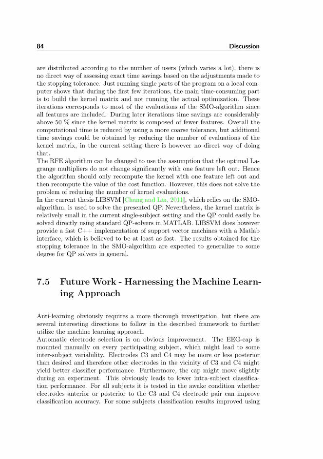
84 Discussion
are distributed according to the number of users (which varies a lot), there isno direct way of assessing exact time savings based on the adjustments made tothe stopping tolerance. Just running single parts of the program on a local com-puter shows that during the first few iterations, the main time-consuming partis to build the kernel matrix and not running the actual optimization. Theseiterations corresponds to most of the evaluations of the SMO-algorithm sinceall features are included. During later iterations time savings are considerablyabove 50 % since the kernel matrix is composed of fewer features. Overall thecomputational time is reduced by using a more coarse tolerance, but additionaltime savings could be obtained by reducing the number of evaluations of thekernel matrix, in the current setting there is however no direct way of doingthat.The RFE algorithm can be changed to use the assumption that the optimal La-grange multipliers do not change significantly with one feature left out. Hencethe algorithm should only recompute the kernel with one feature left out andthen recompute the value of the cost function. However, this does not solve theproblem of reducing the number of kernel evaluations.In the current thesis LIBSVM [Chang and Lin, 2011], which relies on the SMO-algorithm, is used to solve the presented QP. Nevertheless, the kernel matrix isrelatively small in the current single-subject setting and the QP could easily besolved directly using standard QP-solvers in MATLAB. LIBSVM does howeverprovide a fast C++ implementation of support vector machines with a Matlabinterface, which is believed to be at least as fast. The results obtained for thestopping tolerance in the SMO-algorithm are expected to generalize to somedegree for QP solvers in general.
7.5 Future Work - Harnessing the Machine Learn-ing Approach
Anti-learning obviously requires a more thorough investigation, but there areseveral interesting directions to follow in the described framework to furtherutilize the machine learning approach.Automatic electrode selection is on obvious improvement. The EEG-cap ismounted manually on every participating subject, which might lead to someinter-subject variability. Electrodes C3 and C4 may be more or less posteriorthan desired and therefore other electrodes in the vicinity of C3 and C4 mightyield better classifier performance. Furthermore, the cap might move slightlyduring an experiment. This obviously leads to lower intra-subject classifica-tion performance. For all subjects it is tested in the awake condition whetherelectrodes anterior or posterior to the C3 and C4 electrode pair can improveclassification accuracy. For some subjects classification results improved using

7.5 Future Work - Harnessing the Machine Learning Approach 85
more posterior electrodes in the awake case, but it was not consistently a goodindication of what electrodes worked best for the sleep data. Combining therelation between the most important electrodes in the awake condition however,could lead to additional insights and further weight could be given to the ob-tained results if electrodes selected automatically in the awake condition couldbe transferred to the sleeping condition.Ideally, a framework where the most important electrodes for the classificationare determined automatically using the data should be built. The most informa-tive electrodes could be selected using either a clustering algorithm or a commonspatial pattern on the full set of electrodes. This would both reduce the influ-ence of electrode-cap placement and reduce inter-subject variability. FieldTripsclustering algorithm was tested on the data-set, and did indeed find C3, C4,CP3, and CP4 to be the most relevant electrodes in most cases. Hence it wouldbe a good path to follow.Inspired by the presented approach to feature elimination the method can beexpanded to include a recursive channel elimination step where channels are re-moved iteratively in a similar fashion to the recursive feature elimination. Thiswould reduce the inclusion of prior knowledge, which, as discussed, can be mis-leading for new experimental paradigms. Furthermore, it would automaticallyfind the most relevant brain areas for the classification. This would require alower dimensional feature space for each channel, which could be achieved byusing e.g. autoregressive coefficients as proposed in [Lal et al., 2004].The artifact rejection should be automatized to a higher degree to reduce humanbias and inconsistency. Using a toolbox like CORRMAP[Campos Viola et al.,2009], would allow the identification and clustering of independent componentsrepresenting EEG artifacts. Finally, finding a good data representation is keyand there are several parameters to investigate further, likewise more advancedmethods can be adopted which can deal with variable latencies in data derivedfrom neural activity. Multilinear shift-invariant decompositions can handle thisto some degree [Mørup et al., 2008].

86 Discussion
Chapter 8
Conclusion
The results obtained in the present thesis indicate that the sleeping human brainis responsive to external auditory input and indeed capable of processing it ata semantic level.Discriminative activity is found in at least 12 out of the 18 subjects duringsleep. Using the proposed method during wakefulness, it is possible to showdiscriminative activity in 16 out of 18 subjects.It remains a question whether the observation generalizes to all sleep stages,and to elucidate the degree of motor cortex involvement. Furthermore, it isless clear where in the process from semantic processing to actual execution theobstruction of neural signals occur.
A novel framework for analyzing EEG-recordings has been presented in a chal-lenging context of low sample high dimensional data. The challenge is magnifiedby the low signal-to-noise ratio from the unexplored experimental paradigm in-vestigating the degree of semantic processing during sleep. The proposed frame-work gives a way of analyzing whether discriminative patterns are present in therecorded EEG signals, and where the information is located at a single-subjectlevel. The method succeeds regardless of effective behavioral response which isgenerally absent during sleep.The engine of the proposed framework is a non-linear SVM with a RBF kernelcombined with an RFE algorithm. The presented implementation is a modi-fied and improved algorithm, where parameters are re-estimated during every
88 Conclusion
iteration according to a heuristic based on the structure of the feature subset.Even in the low sample size setting, the non-linear capabilities are utilized andnon-linear decision boundaries are found to improve classification.In addition to improved classification performance, the RFE algorithm givesthe possibility to investigate a reduced subset of features driving the classifier.This makes the method especially powerful in new paradigms with no or fewcertain priors established. The results obtained from the feature selection showa large degree of inter-subject variability regarding latency and morphology ofbrain activity. Anyhow, the results are somewhat similar to what is found inclassical ERP and ERD studies of EEG in awake motor-studies. This indicatesthat the brain prepares a relevant response all the way up to motor preparationduring light sleep though execution is clearly suppressed. Since classificationwas possible using other electrode pairs than those of motor areas, this needsfurther investigation of source localization. Superior classification performancewas however obtained in motor areas indicating a relation to the origin of thesignal.
In contrast to the full spectral transform obtained for all channels, a very sparserepresentation giving good performance is found using a more coarse Morletwavelet transform only including channels C3 and C4.Compared to classical statistical analysis, the method excels by the fact thateven for the low sample size setting multivariate analysis is possible at the indi-vidual subject level where classical analysis can only be done at a group level.Along with the sparse data representation, computational tractability was im-proved by adjusting the stopping tolerance of the SMO algorithm during theRFE-loop. This was shown to improve speed without jeopardizing accuracy.From the classifier learning curves found in the single-subject analyses, it is clearthat classification performance in general would benefit from more experimentaltrials.Anti-learning was observed, especially in the data obtained from the visual cor-tex, but plausible explanations have been given. For the awake condition it hasbeen shown how addition of features can reduce anti-learning, and in some caseseven change anti-learning to learning.
SVMs combined with embedded feature selection schemes show some generalencouraging characteristics in relation to interpretation of EEG recorded neuro-scientific data collected in new as well as well-known experimental paradigms.Using a margin-based recursive feature elimination algorithm, it is possible toclassify and characterize discriminative brain activity based on full spectrogramsat a sensor level for single subjects.

Appendix A
Classifier Performance andSpectro-histo-grams

90 Classifier Performance and Spectro-histo-grams
0 10 20 30 40 50 60 70 80 90 100
20
30
40
50
60
70
80
# Features
Err
or
Sleep (−−ICA) Awake Visual Perm
Time (s)
Fre
qu
en
cy (
Hz)
0 0.5 1 1.5 2
5
10
15
20
25
30
35
40
50
100
150
200
250
(a) Electrode C3
Time (s)
Fre
qu
en
cy (
Hz)
0 0.5 1 1.5 2
5
10
15
20
25
30
35
40
50
100
150
200
250
300
(b) Electrode C4
Figure A.1: Subject 105. Top 50 time-frequency features selected duringeach leave-two-out iteration for subject 105. The number of times a feature isselected gives an indication of how important the single features are.
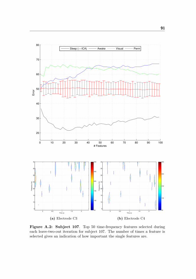
91
0 10 20 30 40 50 60 70 80 90 100
20
30
40
50
60
70
80
# Features
Err
or
Sleep (−−ICA) Awake Visual Perm
Time (s)
Fre
qu
en
cy (
Hz)
0 0.5 1 1.5 2
5
10
15
20
25
30
35
40
50
100
150
200
250
300
(a) Electrode C3
Time (s)
Fre
qu
en
cy (
Hz)
0 0.5 1 1.5 2
5
10
15
20
25
30
35
40
50
100
150
200
250
(b) Electrode C4
Figure A.2: Subject 107. Top 50 time-frequency features selected duringeach leave-two-out iteration for subject 107. The number of times a feature isselected gives an indication of how important the single features are.

92 Classifier Performance and Spectro-histo-grams
0 10 20 30 40 50 60 70 80 90 100
20
30
40
50
60
70
80
# Features
Err
or
Sleep (−−ICA) Awake Visual Perm
Time (s)
Fre
qu
en
cy (
Hz)
0 0.5 1 1.5 2
5
10
15
20
25
30
35
40
50
100
150
200
250
300
(a) Electrode C3
Time (s)
Fre
qu
en
cy (
Hz)
0 0.5 1 1.5 2
5
10
15
20
25
30
35
40
50
100
150
200
250
(b) Electrode C4
Figure A.3: Subject 109. Top 50 time-frequency features selected duringeach leave-two-out iteration for subject 109. The number of times a feature isselected gives an indication of how important the single features are.

93
0 10 20 30 40 50 60 70 80 90 100
20
30
40
50
60
70
80
# Features
Err
or
Sleep (−−ICA) Awake Visual Perm
Time (s)
Fre
qu
en
cy (
Hz)
0 0.5 1 1.5 2
5
10
15
20
25
30
35
40
20
40
60
80
100
120
140
(a) Electrode C3
Time (s)
Fre
qu
en
cy (
Hz)
0 0.5 1 1.5 2
5
10
15
20
25
30
35
40
50
100
150
200
250
(b) Electrode C4
Figure A.4: Subject 111. Top 50 time-frequency features selected duringeach leave-two-out iteration for subject 111. The number of times a feature isselected gives an indication of how important the single features are.
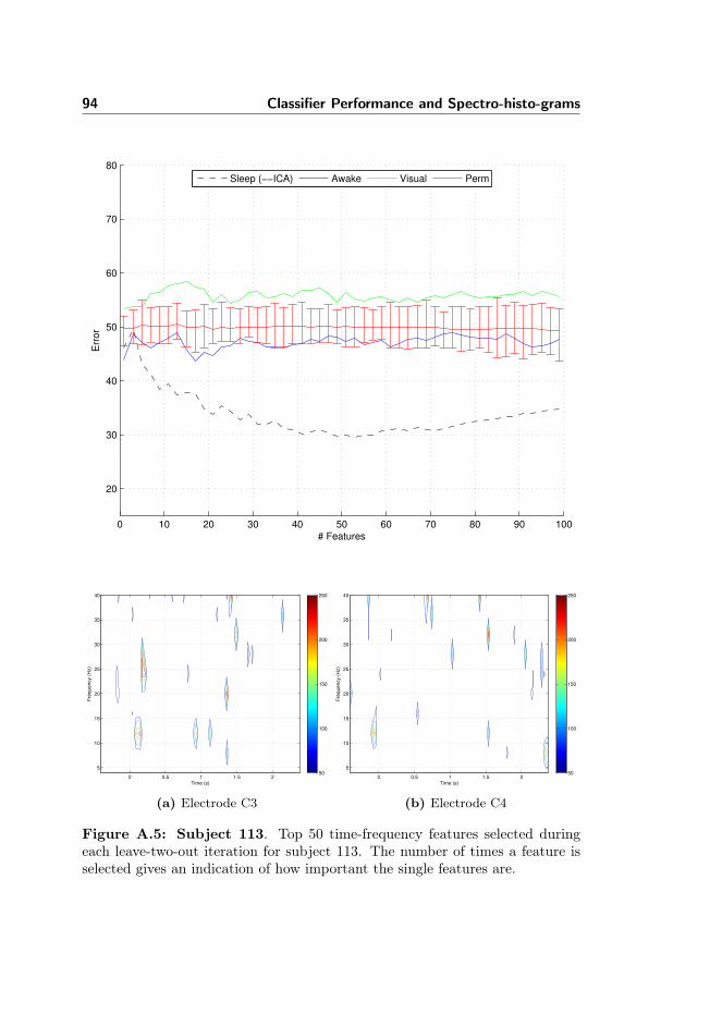
94 Classifier Performance and Spectro-histo-grams
0 10 20 30 40 50 60 70 80 90 100
20
30
40
50
60
70
80
# Features
Err
or
Sleep (−−ICA) Awake Visual Perm
Time (s)
Fre
qu
en
cy (
Hz)
0 0.5 1 1.5 2
5
10
15
20
25
30
35
40
50
100
150
200
250
(a) Electrode C3
Time (s)
Fre
qu
en
cy (
Hz)
0 0.5 1 1.5 2
5
10
15
20
25
30
35
40
50
100
150
200
250
(b) Electrode C4
Figure A.5: Subject 113. Top 50 time-frequency features selected duringeach leave-two-out iteration for subject 113. The number of times a feature isselected gives an indication of how important the single features are.

95
0 10 20 30 40 50 60 70 80 90 100
20
30
40
50
60
70
80
# Features
Err
or
Sleep (−−ICA) Awake Visual Perm
Time (s)
Fre
qu
en
cy (
Hz)
0 0.5 1 1.5 2
5
10
15
20
25
30
35
40
50
100
150
200
250
300
(a) Electrode C3
Time (s)
Fre
qu
en
cy (
Hz)
0 0.5 1 1.5 2
5
10
15
20
25
30
35
40
50
100
150
200
250
(b) Electrode C4
Figure A.6: Subject 122. Top 50 time-frequency features selected duringeach leave-two-out iteration for subject 122. The number of times a feature isselected gives an indication of how important the single features are.

96 Classifier Performance and Spectro-histo-grams
0 10 20 30 40 50 60 70 80 90 100
20
30
40
50
60
70
80
# Features
Err
or
Sleep (−−ICA) Awake Visual Perm
Time (s)
Fre
qu
en
cy (
Hz)
0 0.5 1 1.5 2
5
10
15
20
25
30
35
40
50
100
150
200
250
(a) Electrode C3
Time (s)
Fre
qu
en
cy (
Hz)
0 0.5 1 1.5 2
5
10
15
20
25
30
35
40
50
100
150
200
250
(b) Electrode C4
Figure A.7: Subject 127. Top 50 time-frequency features selected duringeach leave-two-out iteration for subject 127. The number of times a feature isselected gives an indication of how important the single features are.
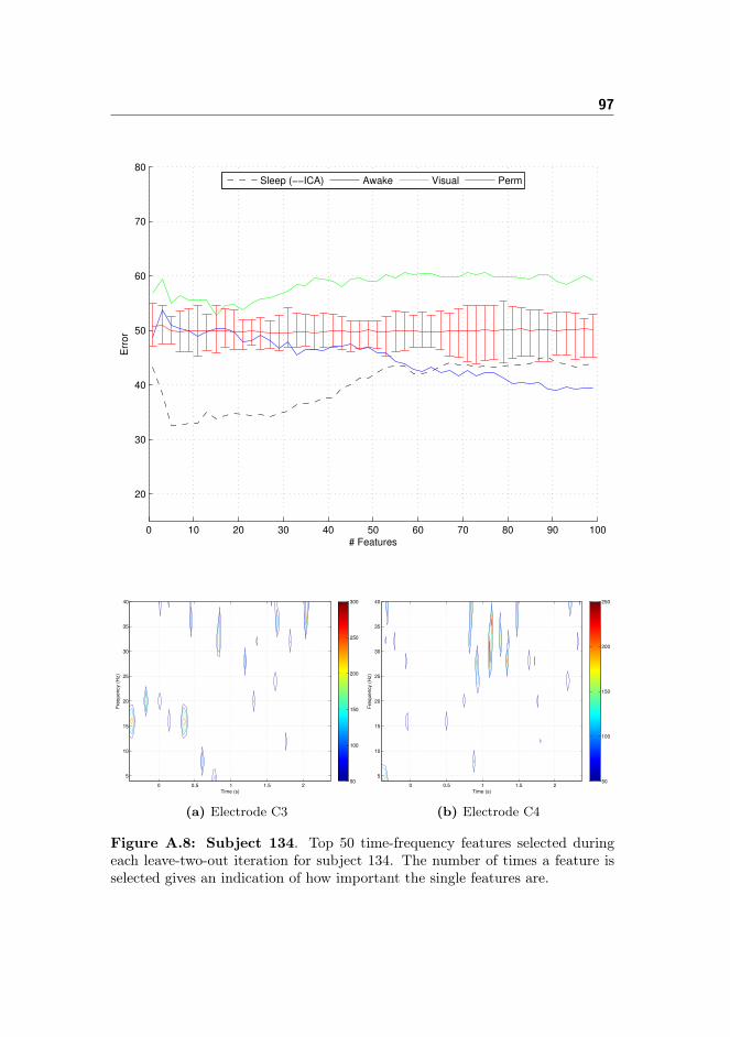
97
0 10 20 30 40 50 60 70 80 90 100
20
30
40
50
60
70
80
# Features
Err
or
Sleep (−−ICA) Awake Visual Perm
Time (s)
Fre
qu
en
cy (
Hz)
0 0.5 1 1.5 2
5
10
15
20
25
30
35
40
50
100
150
200
250
300
(a) Electrode C3
Time (s)
Fre
qu
en
cy (
Hz)
0 0.5 1 1.5 2
5
10
15
20
25
30
35
40
50
100
150
200
250
(b) Electrode C4
Figure A.8: Subject 134. Top 50 time-frequency features selected duringeach leave-two-out iteration for subject 134. The number of times a feature isselected gives an indication of how important the single features are.

98 Classifier Performance and Spectro-histo-grams
0 10 20 30 40 50 60 70 80 90 100
20
30
40
50
60
70
80
# Features
Err
or
Sleep (−−ICA) Awake Visual Perm
Time (s)
Fre
qu
en
cy (
Hz)
0 0.5 1 1.5 2
5
10
15
20
25
30
35
40
50
100
150
200
250
(a) Electrode C3
Time (s)
Fre
qu
en
cy (
Hz)
0 0.5 1 1.5 2
5
10
15
20
25
30
35
40
50
100
150
200
250
(b) Electrode C4
Figure A.9: Subject 137. Top 50 time-frequency features selected duringeach leave-two-out iteration for subject 137. The number of times a feature isselected gives an indication of how important the single features are.

99
0 10 20 30 40 50 60 70 80 90 100
20
30
40
50
60
70
80
# Features
Err
or
Sleep (−−ICA) Awake Visual Perm
Time (s)
Fre
qu
en
cy (
Hz)
0 0.5 1 1.5 2
5
10
15
20
25
30
35
40
50
100
150
200
250
(a) Electrode C3
Time (s)
Fre
qu
en
cy (
Hz)
0 0.5 1 1.5 2
5
10
15
20
25
30
35
40
50
100
150
200
250
(b) Electrode C4
Figure A.10: Subject 138. Top 50 time-frequency features selected duringeach leave-two-out iteration for subject 138. The number of times a feature isselected gives an indication of how important the single features are.

100 Classifier Performance and Spectro-histo-grams
0 10 20 30 40 50 60 70 80 90 100
20
30
40
50
60
70
80
# Features
Err
or
Sleep (−−ICA) Awake Visual Perm
Time (s)
Fre
qu
en
cy (
Hz)
0 0.5 1 1.5 2
5
10
15
20
25
30
35
40
50
100
150
200
250
300
(a) Electrode C3
Time (s)
Fre
qu
en
cy (
Hz)
0 0.5 1 1.5 2
5
10
15
20
25
30
35
40
50
100
150
200
250
(b) Electrode C4
Figure A.11: Subject 144. Top 50 time-frequency features selected duringeach leave-two-out iteration for subject 144. The number of times a feature isselected gives an indication of how important the single features are.

101
0 10 20 30 40 50 60 70 80 90 100
20
30
40
50
60
70
80
# Features
Err
or
Sleep (−−ICA) Awake Visual Perm
Time (s)
Fre
qu
en
cy (
Hz)
0 0.5 1 1.5 2
5
10
15
20
25
30
35
40
50
100
150
200
250
(a) Electrode C3
Time (s)
Fre
qu
en
cy (
Hz)
0 0.5 1 1.5 2
5
10
15
20
25
30
35
40
50
100
150
200
250
300
(b) Electrode C4
Figure A.12: Subject 147. Top 50 time-frequency features selected duringeach leave-two-out iteration for subject 147. The number of times a feature isselected gives an indication of how important the single features are.

102 Classifier Performance and Spectro-histo-grams
0 10 20 30 40 50 60 70 80 90 100
20
30
40
50
60
70
80
# Features
Err
or
Sleep (−−ICA) Awake Visual Perm
Time (s)
Fre
qu
en
cy (
Hz)
0 0.5 1 1.5 2
5
10
15
20
25
30
35
40
50
100
150
200
250
(a) Electrode C3
Time (s)
Fre
qu
en
cy (
Hz)
0 0.5 1 1.5 2
5
10
15
20
25
30
35
40
50
100
150
200
250
300
(b) Electrode C4
Figure A.13: Subject 149. Top 50 time-frequency features selected duringeach leave-two-out iteration for subject 149. The number of times a feature isselected gives an indication of how important the single features are.
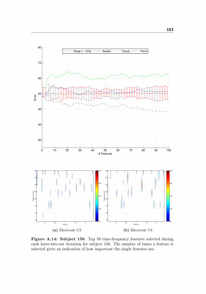
103
0 10 20 30 40 50 60 70 80 90 100
20
30
40
50
60
70
80
# Features
Err
or
Sleep (−−ICA) Awake Visual Perm
Time (s)
Fre
qu
en
cy (
Hz)
0 0.5 1 1.5 2
5
10
15
20
25
30
35
40
50
100
150
200
250
(a) Electrode C3
Time (s)
Fre
qu
en
cy (
Hz)
0 0.5 1 1.5 2
5
10
15
20
25
30
35
40
50
100
150
200
250
(b) Electrode C4
Figure A.14: Subject 150. Top 50 time-frequency features selected duringeach leave-two-out iteration for subject 150. The number of times a feature isselected gives an indication of how important the single features are.

104 Classifier Performance and Spectro-histo-grams
Time (s)
Fre
qu
en
cy (
Hz)
0 0.5 1 1.5 2
5
10
15
20
25
30
35
40
20
40
60
80
100
120
140
(a) Electrode C3
Time (s)F
req
ue
ncy (
Hz)
0 0.5 1 1.5 2
5
10
15
20
25
30
35
40
20
40
60
80
100
120
140
160
(b) Electrode C4
Figure A.15: Subject 134. Top 6 time-frequency features selected duringeach leave-two-out iteration for subject 134.

Appendix B
Learning Curves
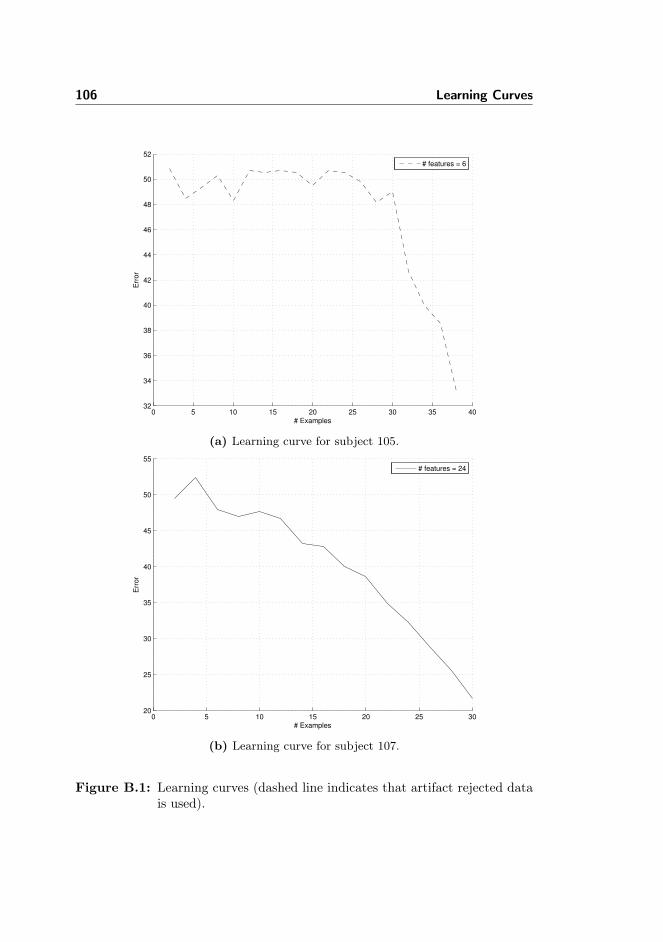
106 Learning Curves
0 5 10 15 20 25 30 35 4032
34
36
38
40
42
44
46
48
50
52
# Examples
Err
or
# features = 6
(a) Learning curve for subject 105.
0 5 10 15 20 25 3020
25
30
35
40
45
50
55
# Examples
Err
or
# features = 24
(b) Learning curve for subject 107.
Figure B.1: Learning curves (dashed line indicates that artifact rejected datais used).
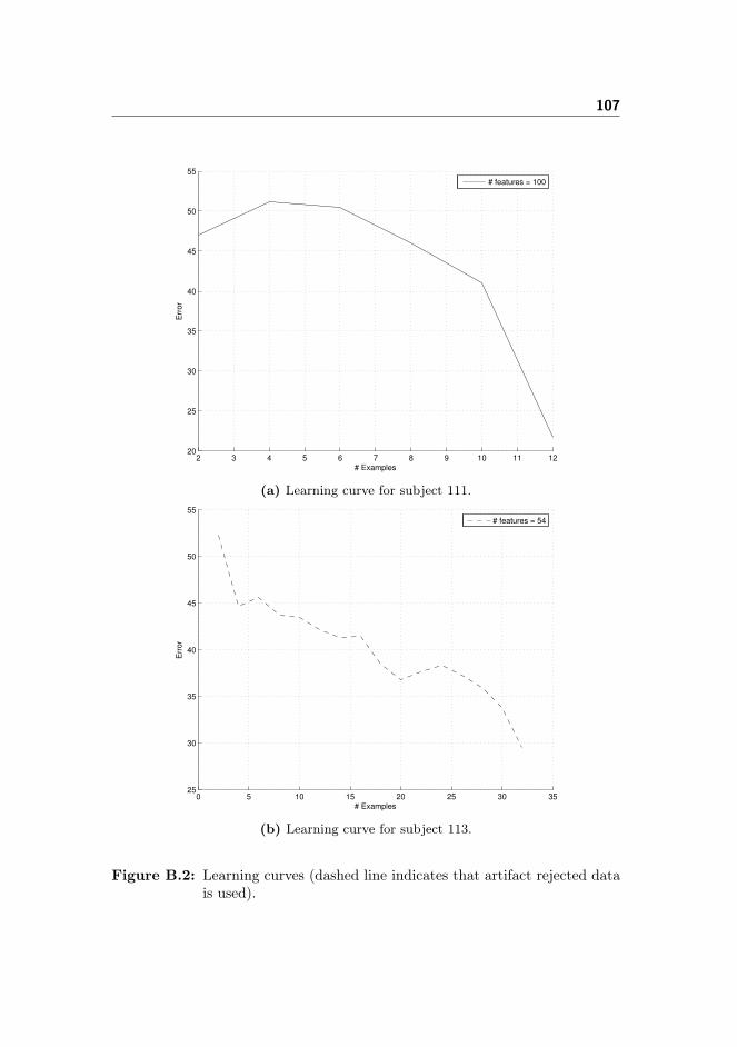
107
2 3 4 5 6 7 8 9 10 11 1220
25
30
35
40
45
50
55
# Examples
Err
or
# features = 100
(a) Learning curve for subject 111.
0 5 10 15 20 25 30 3525
30
35
40
45
50
55
# Examples
Err
or
# features = 54
(b) Learning curve for subject 113.
Figure B.2: Learning curves (dashed line indicates that artifact rejected datais used).

108 Learning Curves
2 4 6 8 10 12 14 1615
20
25
30
35
40
45
50
55
# Examples
Err
or
# features = 60
(a) Learning curve for subject 117.
0 5 10 15 20 25 3025
30
35
40
45
50
55
# Examples
Err
or
# features = 26
(b) Learning curve for subject 122.
Figure B.3: Learning curves (dashed line indicates that artifact rejected datais used).
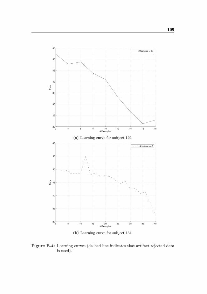
109
2 4 6 8 10 12 14 16 1820
25
30
35
40
45
50
55
# Examples
Err
or
# features = 24
(a) Learning curve for subject 129.
0 5 10 15 20 25 30 35 4030
35
40
45
50
55
60
# Examples
Err
or
# features = 8
(b) Learning curve for subject 134.
Figure B.4: Learning curves (dashed line indicates that artifact rejected datais used).

110 Learning Curves
2 4 6 8 10 12 14 1636
38
40
42
44
46
48
50
52
# Examples
Err
or
# features = 32
(a) Learning curve for subject 138.
2 4 6 8 10 12 14 16 1830
32
34
36
38
40
42
44
46
48
50
# Examples
Err
or
# features = 32
(b) Learning curve for subject 139.
Figure B.5: Learning curves (dashed line indicates that artifact rejected datais used).

111
0 5 10 15 20 25 3025
30
35
40
45
50
55
60
# Examples
Err
or
# features = 26
(a) Learning curve for subject 144.
0 5 10 15 20 25 30 35 40 4538
40
42
44
46
48
50
52
54
# Examples
Err
or
# features = 96
(b) Learning curve for subject 150.
Figure B.6: Learning curves (dashed line indicates that artifact rejected datais used).

112 Learning Curves

Appendix C
Awake ClassifierPerformance

114 Awake Classifier Performance
0 100 200 300 400 500 600 700 800 900 1000
20
30
40
50
60
70
80
# Features
Err
or
Awake Awake ICA
(a) Subject 113.
0 100 200 300 400 500 600 700 800 900 1000
20
30
40
50
60
70
80
# Features
Err
or
Awake Awake ICA
(b) Subject 118.
Figure C.1: Classifier performance with up to 1,000 features included in themodel.
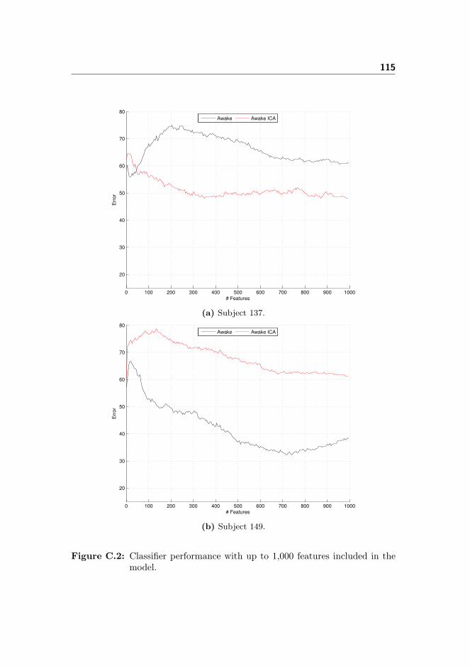
115
0 100 200 300 400 500 600 700 800 900 1000
20
30
40
50
60
70
80
# Features
Err
or
Awake Awake ICA
(a) Subject 137.
0 100 200 300 400 500 600 700 800 900 1000
20
30
40
50
60
70
80
# Features
Err
or
Awake Awake ICA
(b) Subject 149.
Figure C.2: Classifier performance with up to 1,000 features included in themodel.

116 Awake Classifier Performance

Bibliography
[Andrew and Pfurtscheller, 1996] Andrew, C. and Pfurtscheller, G. (1996).Event-related coherence as a tool for studying dynamic interaction of brainregions. Electroencephalography and clinical Neurophysiology, 98(2):144–148.
[Antony et al., 2012] Antony, J., Gobel, E., O’Hare, J., Reber, P., and Paller,K. (2012). Cued memory reactivation during sleep influences skill learning.Nature Neuroscience.
[Aserinsky and Kleitman, 1953] Aserinsky, E. and Kleitman, N. (1953). Regu-larly occurring periods of eye motility, and concomitant phenomena, duringsleep. Science, 118(3062):273–274.
[Ashburner et al., 2008] Ashburner, J., Chen, C., Flandin, G., Henson, R.,Kiebel, S., Kilner, J., Litvak, V., Moran, R., Penny, W., Stephan, K., et al.(2008). Spm8 manual. Functional Imaging Laboratory, Institute of Neurology.
[Atienza et al., 2001] Atienza, M., Cantero, J., and Escera, C. (2001). Auditoryinformation processing during human sleep as revealed by event-related brainpotentials. Clinical Neurophysiology, 112(11):2031–2045.
[Bastuji et al., 2002] Bastuji, H., Perrin, F., and Garcia-Larrea, L. (2002). Se-mantic analysis of auditory input during sleep: studies with event relatedpotentials. International Journal of Psychophysiology, 46(3):243–255.
[Bear et al., 2007] Bear, M., Connors, B., and Paradiso, M. (2007). Neuro-science: Exploring the brain. Lippincott Williams & Wilkins.
[Berger, 1929] Berger, H. (1929). Über das Elektroenkephalogramm des Men-schen. Archiv für Psychiatrie und Nervenkrankheiten, 87:527–570.

118 BIBLIOGRAPHY
[Bishop, 2007] Bishop, C. M. (2007). Pattern Recognition and Machine Learn-ing (Information Science and Statistics). Springer, 1st ed. 2006. corr. 2ndprinting edition.
[Blankertz et al., 2004] Blankertz, B., Muller, K.-R., Curio, G., Vaughan,T. M., Schalk, G., Wolpaw, J. R., Schlogl, A., Neuper, C., Pfurtscheller,G., Hinterberger, T., Schroder, M., and Birbaumer, N. (2004). The bci com-petition 2003: Progress and perspectives in detection and discrimination ofeeg single trials. IEEE Transactions on Biomedical Engineering, 51(6).
[Boser et al., 1992] Boser, B. E., Guyon, I. M., and Vapnik, V. N. (1992). Train-ing algorithm for optimal margin classifiers. Proceedings of the Fifth AnnualACM Workshop on Computational Learning Theory, pages 144–152.
[Brown and Singer, 1993] Brown, A. M. and Singer, W. (1993). Synchronizationof cortical activity and its putative role in information processing and learning.Annual Review of Physiology, 55.
[Brualla et al., 1998] Brualla, J., Romero, M., Serrano, M., and Valdizán, J.(1998). Auditory event-related potentials to semantic priming during sleep.Electroencephalography and Clinical Neurophysiology/Evoked Potentials Sec-tion, 108(3):283–290.
[Bruck et al., 2009] Bruck, D., Ball, M., Thomas, I., and Rouillard, V. (2009).How does the pitch and pattern of a signal affect auditory arousal thresholds?Journal of Sleep Research, 18(2):196–203.
[Burton et al., 1988] Burton, S., Harsh, J., and Badia, P. (1988). Cognitiveactivity in sleep and responsiveness to external stimuli. Sleep: Journal ofSleep Research & Sleep Medicine.
[Campos Viola et al., 2009] Campos Viola, F., Thorne, J., Edmonds, B.,Schneider, T., Eichele, T., and Debener, S. (2009). Semi-automatic iden-tification of independent components representing eeg artifact. Clinical Neu-rophysiology, 120(5):868–877.
[Caputo et al., 2002] Caputo, B., Sim, K., Furesjo, F., and Smola, A. (2002).Appearance-based object recognition using svms: Which kernel should i use?In Proc of NIPS workshop on Statistical methods for computational experi-ments in visual processing and computer vision, Whistler, volume 2002.
[Chang and Lin, 2011] Chang, C.-C. and Lin, C.-J. (2011). LIBSVM: A libraryfor support vector machines. ACM Transactions on Intelligent Systems andTechnology, 2(3):27:1–27:27.
[Chapelle et al., 2005] Chapelle, O., Smola, A., Ong, C. S., and Kowalczyk, A.(2005). Data mining unlearnable data sets. Patent Application Publication,US20080027886.

BIBLIOGRAPHY 119
[Chen et al., 2006] Chen, P., Fan, R., and Lin, C. (2006). A study on smo-typedecomposition methods for support vector machines. Neural Networks, IEEETransactions on, 17(4):893–908.
[Cortes and Vapnik, 1995] Cortes, C. and Vapnik, V. (1995). Support-vectornetworks. Machine Learning, 20:273–297.
[Crone et al., 1998] Crone, N. E., Miglioretti, D. L., Gordon, B., Sieracki, J. M.,Wilson, M. T., Uematsu, S., and Lesser, R. P. (1998). Functional mappingof human sensorimotor cortex with electrocorticographic spectral analysis: I.alpha and beta event-related desynchronization. Brain, 121(12):2271–2299.
[Cruse et al., 2011] Cruse, D., Chennu, S., Chatelle, C., Bekinschtein, T.,Fernández-Espejo, D., Pickard, J., Laureys, S., and Owen, A. (2011). Bedsidedetection of awareness in the vegetative state: a cohort study. The Lancet.
[Cruse et al., 2012] Cruse, D., Chennu, S., Chatelle, C., Fernández-Espejo, D.,Bekinschtein, T., Pickard, J., Laureys, S., and Owen, A. (2012). Relation-ship between etiology and covert cognition in the minimally conscious state.Neurology.
[Delorme and Makeig, 2004] Delorme, A. and Makeig, S. (2004). Eeglab: anopen source toolbox for analysis of single-trial eeg dynamics including inde-pendent component analysis. Journal of neuroscience methods, 134(1):9–21.
[Donner et al., 2009] Donner, T. H., Siegel, M., Fries, P., and Engel, A. K.(2009). Buildup of choice-predictive activity in human motor cortex duringperceptual decision making. Current Biology, 19(18):1581–1585.
[Edeline et al., 2000] Edeline, J., Manunta, Y., and Hennevin, E. (2000). Audi-tory thalamus neurons during sleep: changes in frequency selectivity, thresh-old, and receptive field size. Journal of neurophysiology, 84(2):934–952.
[Efron and Tibshirani, 1993] Efron, B. and Tibshirani, R. (1993). An introduc-tion to the bootstrap, volume 57. Chapman & Hall/CRC.
[Emmons and Simon, 1956] Emmons, W. and Simon, C. (1956). The non-recallof material presented during sleep. American Journal of Psychology, 69(1):76–81.
[Fan et al., 2005] Fan, R.-E., Chen, P.-H., and Lin, C.-J. (2005). Working setselection using second order information for training support vector machines.J. Mach. Learn. Res., 6:1889–1918.
[Federmeier and Kutas, 2009] Federmeier, M. and Kutas, K. D. (2009). N400.Scholarpedia, 4(10):7790.

120 BIBLIOGRAPHY
[Formby, 1967] Formby, D. (1967). Maternal recognition of infant’s cry. Devel-opmental medicine and child neurology., 9(3):293–298.
[Golland and Fischl, 2003] Golland, P. and Fischl, B. (2003). Permutation testsfor classification: towards statistical significance in image-based studies. InInformation processing in medical imaging, pages 330–341. Springer.
[Golland et al., 2005] Golland, P., Liang, F., Mukherjee, S., and Panchenko, D.(2005). Permutation tests for classification. Learning Theory, pages 36–39.
[Guyon and Elisseeff, 2003] Guyon, I. and Elisseeff, A. (2003). An introductionto variable and feature selection. J. Mach. Learn. Res., 3:1157–1182.
[Guyon et al., 2004] Guyon, I., Gunn, S., Ben-Hur, A., and Dror, G. (2004).Result analysis of the nips 2003 feature selection challenge. Advances inNeural Information Processing Systems, 17:545–552.
[Guyon et al., 1998] Guyon, I., Makhoul, J., Schwartz, R., and Vapnik, V.(1998). What size test set gives good error rate estimates? Pattern Analysisand Machine Intelligence, IEEE Transactions on, 20(1):52–64.
[Guyon et al., 2002] Guyon, I., Weston, J., Barnhill, S., and Vapnik, V. (2002).Gene selection for cancer classification using support vector machines. Ma-chine Learning, 46(1-3):389–422.
[Guyon et al., 2006] Guyon, I. M., Gunn, S. R., Nikravesh, M., and Zadeh, L.(2006). Feature Extraction, Foundations and Applications. Springer.
[Hall et al., 2005] Hall, P., Marron, J., and Neeman, A. (2005). Geometric rep-resentation of high dimension, low sample size data. Journal of the RoyalStatistical Society: Series B (Statistical Methodology), 67(3):427–444.
[Halperin and Iorio, 1981] Halperin, J. M. and Iorio, L. C. (1981). Responsivityof rats to neutral and danger-signaling stimuli during sleep. Behavioral andNeural Biology, 33(2):213–219.
[Haussler, 1999] Haussler, D. (1999). Convolution Kernels on Discrete Struc-tures. Technical report, University of California at Santa Cruz.
[Haynes and Rees, 2006] Haynes, J. and Rees, G. (2006). Decoding mentalstates from brain activity in humans. Nature Reviews Neuroscience, 7(7):523–534.
[Hennevin et al., 2007] Hennevin, E., Huetz, C., and Edeline, J. (2007). Neu-ral representations during sleep: from sensory processing to memory traces.Neurobiology of learning and memory, 87(3):416–440.
BIBLIOGRAPHY 121
[Holmes et al., 1996] Holmes, A., Blair, R., Watson, G., and Ford, I. (1996).Nonparametric analysis of statistic images from functional mapping experi-ments. Journal of Cerebral Blood Flow & Metabolism, 16(1):7–22.
[Hoogenboom et al., 2006] Hoogenboom, N., Schoffelen, J., Oostenveld, R.,Parkes, L., and Fries, P. (2006). Localizing human visual gamma-band activ-ity in frequency, time and space. Neuroimage, 29(3):764–773.
[Hsu and Lin, 2002] Hsu, C.-W. and Lin, C.-J. (2002). A simple decompositionmethod for support vector machines. Mach. Learn., 46(1-3):291–314.
[Huxley, 1932] Huxley, A. (1932). Brave New World. Chatto & Windus.
[Ibáñez et al., 2008] Ibáñez, A., San Martín, R., Hurtado, E., and López, V.(2008). Methodological considerations related to sleep paradigm using eventrelated potentials. Biological Research, 41(3):271–275.
[Iber, 2007] Iber, C. (2007). The AASM manual for the scoring of sleep andassociated events: rules, terminology and technical specifications. AmericanAcademy of Sleep Medicine.
[Joachims, 1999] Joachims, T. (1999). Making large-scale support vector ma-chine learning practical. In Schölkopf, B., Burges, C. J. C., and Smola, A. J.,editors, Advances in kernel methods, pages 169–184. MIT Press, Cambridge,MA, USA.
[Johns et al., 1991] Johns, M. et al. (1991). A new method for measuring day-time sleepiness: the epworth sleepiness scale. sleep, 14(6):540–545.
[Keerthi and Gilbert, 2002] Keerthi, S. and Gilbert, E. (2002). Convergenceof a generalized smo algorithm for svm classifier design. Machine Learning,46(1):351–360.
[Keerthi and Lin, 2003] Keerthi, S. and Lin, C. (2003). Asymptotic behav-iors of support vector machines with gaussian kernel. Neural computation,15(7):1667–1689.
[Keerthi et al., 2001] Keerthi, S., Shevade, S., Bhattacharyya, C., and Murthy,K. (2001). Improvements to platt’s smo algorithm for svm classifier design.Neural Computation, 13(3):637–649.
[Klement et al., 2008] Klement, S., Madany Mamlouk, A., and Martinetz, T.(2008). Reliability of cross-validation for svms in high-dimensional, low sam-ple size scenarios. Artificial Neural Networks-ICANN 2008, pages 41–50.
[Kouider and Dehaene, 2007] Kouider, S. and Dehaene, S. (2007). Levels ofprocessing during non-conscious perception: a critical review of visual mask-ing. Philosophical Transactions of the Royal Society B: Biological Sciences,362(1481):857–875.
122 BIBLIOGRAPHY
[Kowalczyk, 2007] Kowalczyk, A. (2007). Classification of anti-learnable bio-logical and synthetic data. Knowledge Discovery in Databases: PKDD 2007,pages 176–187.
[Kowalczyk and Chapelle, 2005] Kowalczyk, A. and Chapelle, O. (2005). Ananalysis of the anti-learning phenomenon for the class symmetric polyhedron.In Algorithmic Learning Theory, pages 78–91. Springer.
[Kowalczyk et al., 2007] Kowalczyk, A., Greenawalt, D., Bedo, J., Duong, C.,Raskutti, G., Thomas, R., and Phillips, W. (2007). Validation of anti-learnable signature in classification of response to chemoradiotherapy inesophageal adenocarcinoma patients. In Proc. Intern. Symp. on Optimiza-tion and Systems Biology, OSB (to appear. Citeseer.
[Kramer et al., 1982] Kramer, M., Kinney, L., and Scharf, M. (1982). Dreamincorporation and dream function. Sleep, 82:369–371.
[Kutas and Federmeier, 2011] Kutas, M. and Federmeier, K. (2011). Thirtyyears and counting: Finding meaning in the n400 component of the event-related brain potential (erp). Annual review of psychology, 62:621–647.
[Lal et al., 2004] Lal, T., Schroder, M., Hinterberger, T., Weston, J., Bogdan,M., Birbaumer, N., and Scholkopf, B. (2004). Support vector channel selectionin bci. Biomedical Engineering, IEEE Transactions on, 51(6):1003–1010.
[Lotte et al., 2007] Lotte, F., Congedo, M., Lécuyer, A., Lamarche, F., andArnaldi, B. (2007). A review of classification algorithms for eeg-based brain–computer interfaces. Journal of Neural Engineering, 4(2):R1.
[Manganotti et al., 2004] Manganotti, P., Fuggetta, G., and Fiaschi, A. (2004).Changes of motor cortical excitability in human subjects from wakefulnessto early stages of sleep: a combined transcranial magnetic stimulation andelectroencephalographic study. Neuroscience letters, 362(1):31–34.
[Maquet et al., 2000] Maquet, P. et al. (2000). Functional neuroimaging of nor-mal human sleep by positron emission tomography. Journal of Sleep Research,9(3):207–232.
[Mercer, 1909] Mercer, J. (1909). Functions of positive and negative type andtheir connection with the theory of integral equations. Philos. Trans. RoyalSoc. (A), 83(559):69–70.
[Mitra and Pesaran, 1999] Mitra, P. and Pesaran, B. (1999). Analysis of dy-namic brain imaging data. Biophysical journal, 76(2):691–708.
[Morash et al., 2008] Morash, V., Bai, O., Furlani, S., Lin, P., and Hallett,M. (2008). Classifying eeg signals preceding right hand, left hand, tongue,and right foot movements and motor imageries. Clinical Neurophysiology,119(11):2570–2578.

BIBLIOGRAPHY 123
[Mørup et al., 2007] Mørup, M., Hansen, L., and Arnfred, S. (2007). Erpwave-lab: A toolbox for multi-channel analysis of time–frequency transformed eventrelated potentials. Journal of neuroscience methods, 161(2):361–368.
[Mørup et al., 2008] Mørup, M., Hansen, L., Arnfred, S., Lim, L., and Madsen,K. (2008). Shift-invariant multilinear decomposition of neuroimaging data.NeuroImage, 42(4):1439–1450.
[Muzur et al., 2002] Muzur, A., Pace-Schott, E., and Hobson, J. (2002). Theprefrontal cortex in sleep. Trends in Cognitive Sciences, 6(11):475–481.
[Nocedal and Wright, 1999] Nocedal, J. and Wright, S. (1999). Numerical op-timization. Springer.
[Nofzinger et al., 2002] Nofzinger, E., Buysse, D., Miewald, J., Meltzer, C.,Price, J., Sembrat, R., Ombao, H., Reynolds, C., Monk, T., Hall, M., et al.(2002). Human regional cerebral glucose metabolism during non-rapid eyemovement sleep in relation to waking. Brain, 125(5):1105–1115.
[Norman et al., 2006] Norman, K., Polyn, S., Detre, G., and Haxby, J. (2006).Beyond mind-reading: multi-voxel pattern analysis of fmri data. Trends incognitive sciences, 10(9):424–430.
[Nunez and Srinivasan, 2006] Nunez, P. and Srinivasan, R. (2006). Electricfields of the brain: the neurophysics of EEG. Oxford University Press, USA.
[Oostenveld et al., 2011] Oostenveld, R., Fries, P., Maris, E., and Schoffelen,J. (2011). Fieldtrip: open source software for advanced analysis of meg,eeg, and invasive electrophysiological data. Computational intelligence andneuroscience, 2011:1.
[Oswald et al., 1960] Oswald, I., Taylor, A., and Treisman, M. (1960). Discrim-inative responses to stimulation during human sleep. Brain, 83(3):440–&.
[Percival and Walden, 1993] Percival, D. and Walden, A. (1993). Spectral anal-ysis for physical applications: multitaper and conventional univariate tech-niques. Cambridge University Press.
[Pereira et al., 2009] Pereira, F., Mitchell, T., and Botvinick, M. (2009). Ma-chine learning classifiers and fmri: a tutorial overview. Neuroimage,45(1):S199–S209.
[Perrin, 2004] Perrin, F. (2004). Auditory event-related potentials studies ofinformation processing during human sleep. Psychologica belgica, 44:43–58.
[Perrin et al., 1999] Perrin, F., García-Larrea, L., Mauguičre, F., and Bastuji,H. (1999). A differential brain response to the subject’s own name persistsduring sleep. Clinical Neurophysiology, 110(12):2153–2164.

124 BIBLIOGRAPHY
[Pfurtscheller, 1977] Pfurtscheller, G. (1977). Graphical display and statisticalevaluation of event-related desynchronization (erd). Electroencephalographyand Clinical Neurophysiology, 43(5):757–760.
[Pfurtscheller, 1992] Pfurtscheller, G. (1992). Event-related synchronization(ers) - an electrophysiological correlate of cortical areas at rest. Electroen-cephalography and Clinical Neurophysiology, 83(1):62–69.
[Pfurtscheller et al., 2006] Pfurtscheller, G., Brunner, C., Schlögl, A., andLopes da Silva, F. H. (2006). Mu rhythm (de)synchronization and eeg single-trial classification of different motor imagery tasks. Neuroimage, 31(1):153–159.
[Pfurtscheller and Lopes da Silva, 1999] Pfurtscheller, G. and Lopes da Silva,F. H. (1999). Event-related eeg/meg synchronization and desynchronization:basic principles. Clinical Neurophysiology, 110(11):1842–1857.
[Pfurtscheller et al., 1993] Pfurtscheller, G., Neuper, C., and Kalcher, J. (1993).40-hz oscillations during motor behavior in man. Neuroscience letters, 164(1-2):179–182.
[Platt, 1998] Platt, J. (1998). Sequential minimal optimization: A fast algo-rithm for training support vector machines. Technical report, Advances inKernel Methods - Support Vector Learning.
[Polyanin and Manzhirov, 2008] Polyanin, A. D. and Manzhirov, A. V. (2008).Handbook of Integral Equations. Chapman & Hall/CRC Press, 2 edition.
[Radovanović et al., 2010] Radovanović, M., Nanopoulos, A., and Ivanović, M.(2010). Hubs in space: Popular nearest neighbors in high-dimensional data.The Journal of Machine Learning Research, 9999:2487–2531.
[Raghavachari et al., 2001] Raghavachari, S., Kahana, M., Rizzuto, D., Caplan,J., Kirschen, M., Bourgeois, B., Madsen, J., and Lisman, J. (2001). Gatingof human theta oscillations by a working memory task. The journal of Neu-roscience, 21(9):3175–3183.
[Rodenbeck et al., 2006] Rodenbeck, A., Binder, R., Geisler, P., Danker-Hopfe,H., Lund, R., Raschke, F., Weeß, H., and Schulz, H. (2006). A review ofsleep eeg patterns. part i: A compilation of amended rules for their visualrecognition according to rechtschaffen and kales. Somnologie, 10(4):159–175.
[Roth et al., 1956] Roth, M., Shaw, J., and Green, J. (1956). The form, volt-age distribution and physiological significance of the k-complex. Electroen-cephalography and Clinical Neurophysiology, 8(3):385–402.
[Schölkopf and Smola, 2002] Schölkopf, B. and Smola, A. J. (2002). Learningwith kernels : support vector machines, regularization, optimization, and be-yond. The MIT Press, 1st edition.

BIBLIOGRAPHY 125
[Shawe-Taylor and Cristianini, 2004] Shawe-Taylor, J. and Cristianini, N.(2004). Kernel methods for pattern analysis. Cambridge Univ Pr.
[Strother et al., 2002] Strother, S., Anderson, J., Hansen, L., Kjems, U., Kus-tra, R., Sidtis, J., Frutiger, S., Muley, S., LaConte, S., and Rottenberg, D.(2002). The quantitative evaluation of functional neuroimaging experiments:The npairs data analysis framework. NeuroImage, 15(4):747–771.
[Tangermann, 2007] Tangermann, M. (2007). Feature Selection for Brain-Computer Interfaces. PhD thesis, Universitätsbibliothek Tübingen.
[Tangermann et al., 2012] Tangermann, M., Müller, K., Aertsen, A., Bir-baumer, N., Braun, C., Brunner, C., Leeb, R., Mehring, C., Miller, K.,Müller-Putz, G., et al. (2012). Review of the bci competition iv. Frontiers inNeuroscience, 6.
[van Vugt et al., 2007] van Vugt, M., Sederberg, P., and Kahana, M. (2007).Comparison of spectral analysis methods for characterizing brain oscillations.Journal of neuroscience methods, 162(1):49–63.
[Vapnik, 1998] Vapnik, V. N. (1998). Statistical learning theory. Wiley, 1 edi-tion.
[Vapnik, 2000] Vapnik, V. N. (2000). The nature of statistical learning theory.Springer-Verlag New York Inc.
[Vapnik, 2006] Vapnik, V. N. (2006). Estimation of dependences based on em-pirical data. Springer-Verlag New York Inc.