Pattern-forming fronts in a Swift-Hohenberg equation with directional

quenching — parallel and oblique stripes

Ryan Goh and Arnd Scheel

August 12, 2017

Abstract

We study the effect of domain growth on the orientation of striped phases in a Swift-Hohenberg equation.

Domain growth is encoded in a step-like parameter dependence that allows stripe formation in a half plane, and

suppresses patterns in the complement, while the boundary of the pattern-forming region is propagating with

fixed normal velocity. We construct front solutions that leave behind stripes in the pattern-forming region that

are parallel to or at a small oblique angle to the boundary.

Technically, the construction of stripe formation parallel to the boundary relies on ill-posed, infinite-dimensional

spatial dynamics. Stripes forming at a small oblique angle are constructed using a functional-analytic, perturbative

approach. Here, the main difficulties are the presence of continuous spectrum and the fact that small oblique

angles appear as a singular perturbation in a traveling-wave problem. We resolve the former difficulty using

a farfield-core decomposition and Fredholm theory in weighted spaces. The singular perturbation problem is

resolved using preconditioners and boot-strapping.

1 Introduction

We are interested in the growth of crystalline phases in macro- or mesoscopic systems, subject to directional

quenching. More precisely, we are interested in systems that exhibit stable or metastable ordered states, such as

stripes, or spots arranged in hexagonal lattices. Examples of such systems arise for example in di-block copolymers

[12], phase-field models [30, 1], and other phase separative systems [9, 37, 19], as well as in phyllotaxis [27], and

reaction diffusion systems [24, 2]. Throughout, we will focus on a paradigmatic model, the Swift-Hohenberg

equation

ut = −(1 + ∆)2u+ µu− u3, (1.1)

where u = u(t, x, y) ∈ R, (x, y) ∈ R2, t ∈ R, subscripts denote partial derivatives, and ∆u = uxx + uyy. It is well

known that for µ > 0, (1.1) possesses stable striped patterns up(kxx+ kyy; k), with up(θ; k) = up(θ + 2π; k) and

wave vector k = (kx, ky), k = |k| for µ > 0. The wave vector can be thought of as the lattice parameter of the

crystalline phase, encoding its strain and orientation.

The particular scenario of interest here is when such a system is quenched into a pattern-forming state in a

growing half plane (x, y) |x − ct < 0, choosing for instance µ = −µ0 sign (x − ct). The main question is then

if the growth process will select an orientation or strain in the crystalline phase. Roughly speaking, our analysis

establishes such a selection mechanism, for the strain, as a function of an arbitrary orientation, at least for small

oblique angles.

In a moving coordinate frame ξ = x− ct, (1.1) then reads

ut = −(1 + ∆)2u− µ0sign (ξ)u− u3 + cuξ. (1.2)

The growth process and the selection of stripes is encoded in the existence and stability of coherent structures,

that is, traveling waves or time-periodic solutions to (1.2).

1

Stripes parallel to the boundary in a comoving frame are of the form up(kxx; kx) = up(kx(ξ+ ct); kx), hence time-

periodic. The simplest solutions enabling the creation of such stripes are therefore of the form u(ζ, τ), τ = ωt,

ζ = kxξ, ω = ckx, solving the boundary-value problem on (ζ, τ) ∈ R2,−ωuτ − (k2

x∂2ζ + 1)2u+ µ(ζ)u− u3 + ωuζ = 0

u(ζ, τ)− u(ζ, τ + 2π) = 0

limζ→∞ u(ζ, τ) = 0

limζ→−∞ (u(ζ, τ)− up(τ + ζ; kx)) = 0,

(1.3)

for some kx.

Obliques stripes up(kxx + kyy; k) = up(kxξ + kyy + ckxt; k) are stationary in a vertically comoving frame τ =

−(kyy + ckxt). The simplest solutions enabling the creation of oblique stripes are therefore of the form u(ζ, τ),

with ζ = kxξ, τ = −(kyy + ωt), ω = ckx, and solve−ωuτ − (k2

x∂2ζ + k2

y∂2τ + 1)2u+ µ(ζ)u− u3 + ωuζ = 0

u(ζ, τ)− u(ζ, τ + 2π) = 0

limζ→∞ u(ζ, τ) = 0

limζ→−∞ (u(ζ, τ)− up(τ + ζ; k)) = 0,

(1.4)

for some kx. Note that, formally letting ky → 0, the problem (1.4) limits on (1.3). The difficulty in this limiting

process is two-fold. First, the perturbation is singular in that the highest derivatives in τ vanish at ky = 0.

Second, the linearization L of (1.3) at a solution u∗tr,

Lv := −ωvτ − (k2x∂

2ζ + 1)2v + µ(ζ)v − 3(u∗tr)

2v + ωvζ , (1.5)

is not Fredholm as a closed and densely defined operator on L2(R × T), say, where T = R/2πZ. This can be

readily seen noticing that ∂τu∗tr belongs to the kernel but does not converge to zero at infinity, such that a simple

Weyl sequence construction shows that the range is not closed.

It turns out that Fredholm properties can be recovered by choosing exponentially weighted function spaces. We

therefore introduce the space

L2η(R× T) =

u(ζ, τ) ∈ L2

loc(R× T) | eη|ζ|u ∈ L2(R× T), (1.6)

and consider L as a closed operator on this exponentially weighted space with small weights η ∼ 0.

Definition 1.1 (Non-degenerate parallel stripe formation). We say that a solution u∗tr of (1.3) is non-degenerate

if the linearization L is Fredholm of index 0 in the weighted space L2η for all η < 0, sufficiently small, and λ = 0

is algebraically simple as an eigenvalue in these spaces. Moreover, the asymptotic periodic patterns are stable

with respect to coperiodic perturbations, with a simple zero eigenvalue of the coperiodic linearization induced by

translations.

We refer the reader to [33] for background and a spatial dynamics illustration motivating such non-degeneracy

conditions. Note also that this choice of exponential weights allows for exponential growth of functions and is

hence generally ill-suited for nonlinear analysis.

Main results. We are now in a position to state our results. Our first result is concerned with a singular

perturbation in the presence of essential spectrum.

Theorem 1 (Parallel =⇒ oblique stripe formation). Suppose there exists a solution (u∗tr, k∗x) of (1.3) for some

fixed c > 0, µ0 > 0, forming parallel stripes. Suppose furthermore that the solution is non-degenerate as stated in

Definition 1.1. Then there exists a family of solutions (utr, kx) to (1.4), depending on ky ∼ 0, sufficiently small,

forming oblique stripes. At ky = 0, this family coincides with (u∗tr, k∗x). The dependence of kx and of the solutions

utr on ky, measured in C0loc(R × T), is of class C2. At leading order, the wavenumber satisfies the expansion

kx(ky) = k∗x −byck2y +O(k4

y) with by defined in (2.29), below.

Our second result shows that the assumptions of Theorem 1 hold for µ0 > 0, sufficiently small.

2

Theorem 2 (Existence of parallel stripe formation). For all µ0 > 0 sufficient small and 0 < c < c∗(µ0),

c∗(µ0) = 4√µ0 + O(µ0), there exists a kx(c) and solution u∗tr to (1.3) that is non-degenerate in the sense of

Definition 1.1.

Together, these two results establish the existence of crystallization fronts forming stripes with small oblique angle

to the interface x = ct. In particular, crystallization fronts select wavenumbers transverse to the interface, de-

pending on prescribed wavenumbers parallel to the interface. Using that k ∼ 1, one can equivalently parameterize

strain in the crystalline phase as a function of grain orientation, that is, growth selects strain but not orientation

in this case of near-parallel orientation; see Remark 2.8.

We expect non-degeneracy as in Definition 1.1 to hold generically for parallel stripe formation. In particular, we

expect Theorem 1 to apply to parallel stripe formation at finite amplitude, µ0 not necessarily small, or in other

systems exhibiting striped phases, as described above. Theorem 2, on the other hand, is intrinsically focused

on small amplitudes. It seems difficult to obtain existence results of this type at finite amplitude. We expect,

however, that the methods from Theorem 2 could be adapted to find solutions to (1.4), at small amplitude. We

chose the alternative approach from Theorem 1 in order to illustrate the robust continuation from parallel to

oblique stripes, independent of small amplitude assumptions and, to some extent, specific model problems.

Techniques. We next comment on technical aspects of the proofs of Theorems 1 and 2.

The proof of Theorem 2 pairs the somewhat classical techniques of center manifold reduction and normal forms

(see [5]) with heteroclinic matching techniques such as invariant foliations and Melnikov theory in an infinite

dimensional setting. In particular, we perform a center manifold reduction in the spatial dynamical systems for

ξ < 0 and ξ > 0, separately. The parallel striped front is then constructed as a heteroclinic orbit from the

intersection of the unstable manifold of a periodic orbit in the ξ < 0-center manifold with the stable manifold of

the origin in the ξ > 0-center manifold. Since locally the two center manifolds only intersect at the origin, we

construct the heteroclinic by finding intersections of the center-unstable manifold of the periodic orbit in the ξ < 0

dynamics with the stable manifold of the origin in the ξ > 0 dynamics. We use invariant foliations to reduce the

infinite-dimensional nature of the problem, allowing us to project the dynamics onto one of the center manifolds

and obtain a leading order intersection. We then use Melnikov theory and transversality arguments to obtain the

desired heteroclinic. Transversality of the intersection implies non-degeneracy as stated in Definition 1.1.

Traditionally, the two main difficulties in proving a result like Theorem 1 have been addressed using spatial

dynamics. To address the neutral continuous spectrum induced by the asymptotic roll state, one typically uses

spatial dynamics in the ζ-direction. That is one formulates the equation as an (ill-posed) dynamical system

with evolutionary variable ζ and studies roll states as periodic orbits and fronts as heteroclinic orbits. Essential

spectrum corresponds to the lack of hyperbolicity of periodic orbits, and is resolved by focusing on strong stable

foliations.

To address the singular limit ky = 0, one might use spatial dynamics in the direction τ along the growth interface,

formulating the equation as a fast-slow dynamical system in the τ -direction [33, 29]. One would then try to study

bifurcations using a center-manifold reduction or the geometric methods pioneered by Fenichel [7].

Combining these two difficulties seems beyond the scope of spatial dynamics techniques, and we therefore resort

to a more direct functional-analytic approach. To overcome the singularly perturbed nature of the problem, we

use an approach similar to [28], preconditioning the problem with a constant-coefficient linear operator before

applying the Implicit Function Theorem. To resolve the difficulties caused by the continuous spectrum, we use

an ansatz of the form

u = w(ζ, τ) + u∗tr(ζ, τ) + χ(ζ) [up(ζ + τ ; k)− up(k∗xζ/kx + τ ; k∗x)] , (1.7)

to decompose the far-field patterns at ζ = −∞ from the “core” patterns near the interface at ζ = 0. Here, χ

is a smooth, monotone function with χ ≡ 1 for ξ < −2 and χ ≡ 0 for ξ > −1. Having accounted in this way

for changes in the farfield wavenumber, we may require the correction w to be exponentially localized. We then

solve in exponentially localized spaces, where the linearization turns out to be Fredholm of index -1, using the

free parameter kx as a variable to account for the cokernel. As a result, we obtain w and kx as functions of the

remaining free parameter ky using the Implicit Function Theorem after careful preconditioning; see Section 2.

Regularity in ky is obtained via a bootstrapping procedure; see Section 2.5.

3

Outline. We prove Theorems 1 and 2 in Section 2 and 3, respectively. We conclude with a discussion of

applications, extensions, and future directions in Section 4.

Acknowledgements. Research partially supported by the National Science Foundation through the grants

NSF-DMS-1603416 (RG), and NSF-DMS-1612441, NSF-DMS-1311740 (AS), as well as a UMN Doctoral Disser-

tation Fellowship (RG). RG would like to thank C. E. Wayne for useful discussions about this work, as well as

the Institute for Mathematics and its Applications for its kind hospitality during a weeklong visit where some of

this research was performed.

2 From parallel to oblique stripes — proof of Theorem 1

We prove Theorem 1. Section 2.1 collects and reinterprets information on the primary profile u∗tr and the lineariza-

tion. We then describe the functional-analytic setup, in particular the farfield-core decomposition, Section 2.2.

Section 2.3 introduces the second key ingredient to the proof, a nonlinear preconditioning to set up the Implicit

Function Theorem. Section 2.4 concludes the existence proof and Section 2.5 establishes differentiability in ky.

2.1 Properties of the parallel trigger and its linearization

We establish smoothness, exponential convergence, and some properties of the linearization. First, notice that u∗trsolves a pseudo-elliptic equation, such that ∂τu and ∂4

ζu belong to L∞, with a jump at ζ = 0. For ζ 6= 0, u∗tr can

readily seen to be smooth. By assumption, u∗tr converges to the periodic pattern up(ζ + τ ; k∗) as ζ → −∞.

By translation invariance in τ , ∂τu∗tr is bounded and belongs to the kernel of the linearized equation in L2

η, for all

η < 0, but not for η ≥ 0, since kx 6= 0.

Lemma 2.1 (Fredholm crossing). The operator L from (1.5) is Fredholm of index -1 in L2η(R × T) for η > 0,

sufficiently small, with trivial kernel.

Proof. We rely on the characterization of Fredholm indices using Fredholm borders; see [32, 34, 8]. Since the

asymptotic state at ξ = +∞ is linearly stable, its Morse index at ξ = −∞ can be calculated through a homotopy

as follows. We linearize at the asymptotic periodic pattern and find, including a spectral homotopy parameter λ,

−ω(uτ − uζ)− (k2x∂

2ζ + 1)2u+ µ0u− 3u2

p(ζ + τ)u = λu.

A Floquet-Bloch ansatz u(ζ, τ) = ei`τeνxζw(ζ + τ), with w(z) = w(z + 2π), yields the periodic boundary value

problem

λu = −ω(i`− νx)− (k2x(∂z + νx)2 + 1)u+ µ0u− 3u2

p(z)u =: Lp(νx)u− ω(i`− νx)u, z ∈ (0, 2π).

We are interested in spatial eigenvalues νx ∈ C, crossing the imaginary axis, that is, νx ∈ iR. In this case, Lp(νx)

is Hermitian, such that for homotopies λ ≥ 0 we necessarily find νx = i` and Lp(i`)w = λw. Restricting to the

fundamental Floquet domain Imνx ∈ [0, 1), we further conclude νx = ` = 0. This however is impossible for λ > 0

by the assumption of coperiodic stability, and it implies that w = u′p up to scalar multiples for λ = 0, νx = ` = 0.

Inspecting multiplicity of this spatial Floquet multiplier νx = 0, one is looking for a generalized eigenfunction w

solving L′p(0)u′p + ωu′p + Lp(0)w = 0 for w, where L′p denotes the derivative with respect to νx. By the quadratic

dependency on νx, this reduces to Lp(0)w = ωu′p, which in turn is impossible since Lp(0) is self-adjoint. This

proves that there is precisely one zero Floquet exponent for λ = 0 and no Floquet exponent crossings for λ > 0,

which implies that L is Fredholm of index 0 for η < 0, small, and Fredholm of index -1 for η > 0, small. Since

the eigenfunction at λ = 0 is not decaying as ξ → −∞, the kernel is trivial for η > 0.

Lemma 2.2. There are C, δ > 0, such that

‖χ(ζ + ζ0) (u∗tr(ζ/k∗x, τ)− up(ζ + τ ; k∗x)) ‖Hk(R×T) ≤ Ce−δζ0 (2.1)

as ζ0 → +∞, where χ is as in (1.7).

4

Proof. We can rely on spatial dynamics; see for isntance [33]. The asymptotic periodic orbit is hyperbolic

up to the neutral Floquet exponent generated by translations, as seen in Lemma 2.1. Its local stable manifold

is therefore given by the union of strong stable fibers, thus implying exponential convergence. Since the spatial

dynamics can be formulated in spaces of arbitrary regularity, convergence is exponential in spaces with higher

derivatives, too.

2.2 Setup and farfield-core decomposition

We start setting up our fixed point argument by performing a functional analytic farfield-core decomposition. We

start from (1.4),

0 = −(1 + (kx∂ζ)2 + (ky∂τ )2)2u+ µ(ζ)u− u3 + ckx(uζ − uτ ), (ζ, τ) ∈ R× T, (2.2)

with the appropriate boundary conditions stated there. Recall that χ is a smooth cut-off function with χ ≡ 1 for

all ξ < −2 and support contained in (−∞,−1]. Our ansatz is of the form

u = w(ζ, τ) + u∗tr

(k∗xkxζ, τ

)+ χ(ζ)

(up (ζ + τ ; k)− up

(k∗xkxζ + τ ; k∗x

)), (2.3)

where k2 = k2x + k2

y. We consider perturbations w ∈ L2η defined in (1.6), with η > 0 sufficiently small. Note that

we introduced parameter dependence into the trigger front u∗tr by simply scaling appropriately with kx, such that

u∗tr solves L(kx, 0)u∗tr + f(u∗tr) + c(k∗x − kx)∂τu∗tr = 0 for all kx 6= 0.

Let us first consider the non-regularized nonlinear map. Inserting the ansatz (2.3) into (1.4), and setting

L(kx, ky) = −(1 + ∆kx,ky )2 + ckx(∂ζ − ∂τ ), f(u) = µ(ζ)u− u3, ∆kx,ky := (kx∂ζ)2 + (ky∂τ )2,

Φ(k)(ζ, τ) = up(ζ + τ, k)− up(k∗xζ/kx + τ ; k∗x),

we find, suppressing τ, ζ dependence,

0 = L(kx, ky)(u∗tr + w + χΦ(k)) + f(u∗tr + w + χΦ(k))

= L(kx, ky)u∗tr + L(kx, ky)(χΦ(k) + w) + f(u∗tr + w + χΦ(k))

= L(kx, ky)(χΦ(k) + w) + f(u∗tr + w + χΦ(k))− f(u∗tr)− (k∗x − kx)c∂τu∗tr + (L(kx, ky)− L(kx, 0))u∗tr.

From this last line, we can then define the mapping

F (w; k) := [L(kx, ky) + f ′(u∗tr)]w +R(k) +N (w; k), (2.4)

with the w-independent residual term

R(k) = L(kx, ky)(χΦ(k)) + f(u∗tr + χΦ(k))− f(u∗tr) + (kx − k∗x)c∂τu∗tr + (L(kx, ky)− L(kx, 0))u∗tr, (2.5)

and the nonlinear term

N (w; k) = f(u∗tr + χΦ(k) + w)− f(u∗tr + χΦ(k))− f ′(u∗tr)w. (2.6)

Since f(u) = µu− u3, we have

N (w; k) = 3(u∗tr + χΦ(k))2w − 3(u∗tr)2w + 3(u∗tr + χΦ(k))w2 + w3.

Exponential convergence of the primary trigger u∗tr from Lemma 2.2 implies that for k = k∗ := (k∗, 0)T , F is a

locally well-defined nonlinear mapping from the anisotropic Sobolev space Xη := H1(T, L2η(R)) ∩ L2(T, H4

η(R))

to L2η. Indeed, one obtains R(k∗) ∈ L2

η using the exponential convergence of u∗tr to up(|k∗|) and the fact that

L(kx, ky)up(|k|) + f(up(|k|)) = 0. Then, since Xη can readily be seen to be a Banach algebra and up is bounded,

we have that N (w; k) ∈ L2η as well.

The existence assumption of u∗tr implies that F (0,k∗) = 0. Also, we note that the linearization of F in w satisfies

∂wF∣∣∣(0,k∗)

= L := −(1 + (k∗x∂ζ)2)2 + f ′(u∗tr) + ck∗x(∂ζ − ∂τ ),

5

which is closed and densely defined on L2η. We also record for later use that

∂kxF∣∣∣(0,k∗)

= [L(k∗x, 0) + f ′(u∗tr)]χ∂kΦ(k∗)− c∂τu∗tr.

It is readily observed that F is not continuous in k2y as a map from Xη to L2

η as it is not well-defined for

ky 6= 0, due to higher-order terms such as ∂4τ and ∂2

τ (1 + (kx∂ζ)2). We will therefore regularize the equation by

preconditioning with a Fourier multiplier in the next section. We conclude this setup by collecting some properties

of the linearization.

Lemma 2.3. For all η > 0 small, let e∗ span cokerL with 〈e∗, ∂τu∗tr〉L2η

= 1. Algebraic simplicity of the eigenvalue

0 in L2η, η < 0, as in Definition 1.1 then implies that⟨

e∗, ∂kxF∣∣∣(0,k∗x,0)

⟩L2η

6= 0. (2.7)

Proof. We argue as in [22, Lemma 6.3]. Namely, if one assumes that the above inner product is zero, then there

exists w0 ∈ L2η and α ∈ R non-zero such that

Lw0 = α∂kxF = α (L(χ∂kxΦ(k∗))− c∂τu∗tr) .

We then have

L(w0 − αχ∂kxΦ(k∗)) = c∂τu∗tr.

Since w0 is exponentially localized, and ∂kxup ∈ L2−η, we have w0 − αχ∂kxΦ(k∗)) 6= 0 and is a generalized

eigenvector of the kernel element ∂τu∗tr when considered in L2

−η, contradicting the algebraic simplicity.

We also define the L2-adjoint of L for later use,

Lad0 : X0 ⊂ L2 → L2

v 7→ −(1 + (k∗x∂x)2)2v − ck∗x(∂x − ∂τ )v + f ′(u∗tr)v. (2.8)

2.3 Regularization of the nonlinear mapping

To prove Theorem 1, we shall study zeros of the regularized nonlinear mapping

F(w; kx, k2y) :=M(kx, k

2y)F (w; k) : Xη → Xη, (2.9)

with the regularizing operator M(kx, k2y) := (L(k)− id)−1 . The existence and boundedness of such an inverse

can be obtained in L2 by studying the associated Fourier multiplier,

M(kx, k2y)(im, i`) =

(−1− (1− k2

x`2 − k2

ym2)2 + ckxi(`−m)

)−1, m ∈ Z, ` ∈ R,

noticing that the real part of the denominator has real part less than -1 for all m, `. One can then extend

existence to the exponentially weighted space L2η by the use of conjugating isomorphisms u 7→ e±η〈x〉u. More

explicitly one obtains the inverse by first obtaining the inverse on the one-sided weighted spaces L2±η,>, where

L2η,> = u : eηξu ∈ L2 and ∂ξ acts as ∂ξ−η, and then use the fact that L2

η = L2η,>∩L2

−η,> with equivalent norm,

||u||L2η,>∩L

2−η,>

:= ||u||L2η,>

+ ||u||L2−η,>

,

This inverse can also be found to have the continuity properties listed in the following proposition. For ease of

notation in the following we let ε = k2y, κ = kx, and κ∗ = k∗x. Also, since they are in fact functions of ε = k2

y, we

re-define R(κ, ε) = R(k) and N (w;κ, ε) = N (w; k).

Proposition 2.4. For ε ∼ 0, κ ∼ κ∗ 6= 0, and speed c 6= 0, the mappings M(κ, ε) and ∂κM(κ, ε) are well-defined,

bounded, and norm-continuous on Xη × R2 → Xη.

6

Proof. Since we are considering M as a mapping from Xη to itself, it suffices to prove the result on L2η.

Furthermore we prove the result for η = 0 as the result for 0 < η 1 can be obtained as discussed above. Hence,

we consider M : L2 → L2.

We start by considering continuity ofM. Therefore let ε→ ε0, κ→ κ0. For ε0 > 0, continuity is easily established

using smoothness properties of the symbol. We therefore focus on the case ε0 = 0, κ0 = κ∗. We need to show

supm,`|M(κ, ε)(im, i`)− M(κ∗, 0)(im, i`)| → 0.

We decompose

supm,`|M(κ, ε)(im, i`)− M(κ∗, 0)(im, i`)|

≤ supm,`|M(κ, ε)(im, i`)− M(κ∗, ε)(im, i`)|+ sup

m,`|M(κ∗, ε)(im, i`)− M(κ∗, 0)(im, i`)| =: (I) + (II).

To estimate (I), we first define

pκ,ε(m, `) = −1− (1− κ2`2 − εm2)2 + cκi(m+ `),

so that ∣∣∣M(κ, ε)(im, i`)− M(κ∗, ε)(im, i`)∣∣∣ =

∣∣∣∣pκ∗,ε(m, `)− pκ,ε(m, `)pκ∗,ε(m, `)pκ,ε(m, `)

∣∣∣∣= |κ− κ∗|

∣∣∣∣ci(`−m)− (κ2∗ + κ2)(κ∗ + κ)`4 − 2εm2`2(κ∗ + κ)

pκ,ε(m, `)pκ∗,ε(m, `)

∣∣∣∣. |κ− κ∗|

∣∣ci(`−m)− 4κ3∗`

4 − 4κ∗εm2`2∣∣

|pκ∗,ε(m, `)|2, (2.10)

where in the last line we used the fact that κ∗ 6= 0. Then

|pκ∗,ε(m, `)2| = |pκ∗,ε(m, `)|

2 = (1 + (1− κ2∗`− εm2)2)2 + c2κ2

∗(`−m)2,

can be bounded from below by 1 + `8 + ε`6m2 + ε2m4 up to a constant independent of ε. It then readily follows

that the above quotient is bounded uniformly in (κ− κ∗) so that∣∣∣M(κ, ε)(im, i`)− M(κ∗, ε)(im, i`)∣∣∣ . |κ− κ∗|. (2.11)

For (II) we further decompose

M(κ, ε)(im, i`)− M(κ, 0)(im, i`) =pκ∗,ε(m, `)− pκ∗,0(m, `)

pκ∗,ε(m, `)pκ,ε(m, `)

=2εm2(1− κ2`2)

pκ∗,ε(m, `)pκ,ε(m, `)− ε2m4

pκ∗,ε(m, `)pκ,ε(m, `)=: (III) + (IV). (2.12)

For (III) we scale m = ε1/3m and define Ωd = |m|2 + |`|2 > d. By studying the real and imaginary parts of the

product pκ∗,ε(m, `)pκ∗,0(m, `), one finds for (m, `) ∈ Ωd and d sufficiently large

|pκ∗,ε(m, `)pκ∗,0(m, `)| & 1 + `8 + |cκm|(`2m2 + ε1/3m4),

so that

|(III)| =∣∣∣∣ 2ε1/3m2(1− κ2`2)

pκ∗,ε(m, `)pκ,ε(m, `)

∣∣∣∣. ε1/3

2m2κ2`2

1 + `8 + |cκ|`2|m|3 + ε1/3|m|5

≤ Cdε1/3, (2.13)

with constant Cd > 0, independent of ε. Note that here we have used the fact that κ∗ and c are both non-zero.

7

On the complement Ωcd, one bounds the denominator from below by 1 so that

|(III)| ≤ |2ε1/3m2(1− κ2`2)|

. ε1/3(|m|2 + |`|2)

≤ C′dε1/3. (2.14)

A similar argument is used to bound (IV), this time with the scaling m = ε2/5m. Indeed, for (m, `) ∈ Ωd we have

(IV) =

∣∣∣∣ 2ε2/5m4

pκ∗,ε(m, `)pκ,ε(m, `)

∣∣∣∣.ε2/5

m4

1 + `8 + |cκ∗||m|5. (2.15)

Combining the bounds for (III) and (IV) we conclude that the term (II) converges to zero as (κ, ε) → (κ∗, 0) as

desired.

We next turn to the derivative, ∂κM. First ∂κM exists in a neighborhood of (κ∗, ε) and has the expected Fourier

multiplier

∂kM(κ, ε) = −∂κpκ,ε(m, `)pκ,ε(m, `)2

,

where p is defined above. This is obtained by observing

supm,`

∣∣∣∣M(κ, ε)− M(κ0, ε)−∂κpκ0,ε(m, `)

pκ0,ε(m, `)2

(κ− κ0)

∣∣∣∣ · |κ− κ0|−1

= supm,`

∣∣∣∣2(κ+ κ0)`2 − (κ2 + κ20)(κ+ κ0)`4 − 2(κ∗ + κ)ε`2m2 + ci(`−m)

pκ,ε(m, `)pκ0,ε(m, `)− 4κ0(1− κ2

0`2 − εm2)`2 + ci(`−m)

pκ0,ε(m, `)2

∣∣∣∣→ 0

(2.16)

as κ→ κ0, for any ε near 0 and κ0 near κ∗. This convergence is obtained using similar estimates as in (2.10).

To prove continuity in (κ, ε), we proceed in the same way as above, aiming to show

supm,`

∣∣∣∂κM(κ, ε)(im, i`)− ∂κM(κ∗, 0)(im, i`)∣∣∣→ 0, as (κ, ε)→ (κ∗, 0),

and thus once again decompose

supm,`

∣∣∣∂κM(κ, ε)(im, i`)− ∂κM(κ∗, 0)(im, i`)∣∣∣

≤ supm,`|∂κM(κ, ε)(im, i`)− ∂κM(κ∗, ε)(im, i`)|+ sup

m,`|∂κM(κ∗, ε)(im, i`)− ∂κM(κ∗, 0)(im, i`)| =: (I) + (II).

(2.17)

It is readily found that

|∂κM(κ, ε)(im, i`)− ∂κM(κ∗, ε)(im, i`)| =∣∣∣∣∂κpκ,ε(m, `)pκ∗,ε(m, `)

2 − ∂κpκ∗,ε(m, `)pκ,ε(m, `)2

pκ,ε(m, `)2pκ∗,ε(m, `)2

∣∣∣∣.

∣∣∣∣∂κpκ,ε(m, `)(pκ∗,ε(m, `)− pκ,ε(m, `))(pκ∗,ε(m, `) + pκ,ε(m, `))

pκ,ε(m, `)2pκ∗,ε(m, `)2

∣∣∣∣+|∂κpκ∗,ε(m, `)− ∂κpκ,ε(m, `)|

|pκ∗,ε(m, `)2|

.|∂κpκ,ε(m, `)||pκ∗,ε(m, `)− pκ,ε(m, `)||pκ,ε(m, `)||pκ,ε(m, `)pκ∗,ε(m, `)|

+

∣∣∣∣∂κpκ∗,ε(m, `)− ∂κpκ,ε(m, `)pκ∗,ε(m, `)

2

∣∣∣∣=

∣∣4κ`2(1− κ2`2 − εm2) + ci(`−m)∣∣

|pκ∗,ε(m, `)||M(κ, ε)− M(κ∗, ε)|

+ |κ− κ∗||4`2 + 4(κ2 + κκ∗ + κ2

∗)`4 + 4εm2`2|

|pκ∗,ε(m, `)|2

. |κ− κ∗|. (2.18)

8

For (II) we proceed in a similar manner finding

|∂κM(κ∗, ε)(im, i`)− ∂κM(κ∗, 0)(im, i`)| =∣∣∣∣∂κpκ∗,ε(m, `)pκ,0(m, `)2 − ∂κpκ,0(m, `)pκ∗,ε(m, `)

2

pκ∗,ε(m, `)2pκ∗,0(m, `)2

∣∣∣∣.

4κ2∗εm

2`2

|pκ∗,ε(m, `))|2+|∂κpκ,0(m, `)||pκ,0(m, `)|

∣∣∣M(κ∗, ε)− M(κ∗, 0)∣∣∣

. ε. (2.19)

Here we have used the fact that | ∂κpκ,0(m,`)

pκ,0(m,`)| is bounded in (m, `) and the same scaling arguments used above for

continuity of M. Combining the estimates for (I) and (II), we conclude the continuity of ∂κM near (κ∗, 0), thus

finishing the proof of the proposition.

Remark 2.5. We note that M is readily seen to be smooth in ε and κ as long as ε > 0.

We can now conclude the continuity of F = w +M(κ, ε) (w + f ′(u∗tr)w +R(κ, ε) +N (w;κ, ε)) in ε, which shall

allow us to apply the Implicit Function Theorem.

Corollary 2.6. For (κ, ε) ∼ (κ∗, 0), the mapping F : Xη × R2 → Xη is locally well-defined in a neighborhood

of (0;κ∗, 0), smooth in w, C1 in κ, and continuous in ε. Furthermore, the derivatives ∂wF and ∂κF are also

continuous in ε.

Proof. We have that

F(w;κ, ε) =M(κ, ε)[(L(κ, ε)w − w) + w + f ′(u∗tr)w +R(κ, ε) +N (w;κ, ε)

]= w +M(κ, ε)

[w + f ′(u∗tr)w +R(κ, ε) +N (w;κ, ε)

].

We have already shown above that R(κ, ε) and N (w, κ, ε) are exponentially localized, taking values in L2η. A

bootstrapping argument can then be used to obtain higher regularity of u∗tr in τ and ζ. This along with the fact

that Xη is a Banach algebra, implies that R and N take values in Xη. Hence we obtain that F is well-defined

and smooth in w near w = 0.

Then, since

∂κΦ(k) = ∂2up(ζ + τ ; |k|)−2κ

|k|2 + ∂1up(κ∗ζ/κ+ τ ; |k∗|)κ∗κ2ζ,

and

|u∗tr(κ∗ζ/κ, τ)− up(κ∗ζ/κ+ τ ; |k∗|)| → 0

|∂κu∗tr − ∂κup(|k∗|)| =∣∣∣∣∂ξu∗tr(κ∗ζ/κ, τ)

κ∗ζ

κ2− ∂1up(κ∗ζ/κ+ τ ; |k∗|)κ∗ζ

κ2

∣∣∣∣→ 0, (2.20)

exponentially fast as ζ → 0, one can readily show that the derivatives ∂κR and ∂κN are well defined as maps (in

κ and w respectively) and continuous in κ in a neighborhood of (κ∗, 0). The regularity of M in κ then implies

that F is C1 in κ as well. We infer continuity of F in ε by combining Proposition 2.4 with the estimate

‖F(w;κ, ε)−F(w;κ, 0)‖Xη ≤ ‖M(κ, ε)−M(κ, 0)‖Xη→Xη‖w + f ′(u∗tr)w +R(κ, ε) +N (w;κ, ε)‖Xη+ ‖M(κ, 0)‖Xη→Xη‖R(κ, ε) +N (w;κ, ε)−R(κ, 0) +N (w;κ, 0)‖Xη . (2.21)

In a similar manner, we also obtain that

∂wF = I +M(κ, ε)[(1 + f ′(utr))I +R(κ, ε) +N ′(w;κ, ε)

],

∂κF = ∂κM(κ, ε)[(1 + f ′(utr))I +R(κ, ε) +N (w;κ, ε)

]+M(κ, ε) [∂κR(κ, ε) + ∂κN (w;κ, ε)] ,

are continuous in ε.

9

2.4 Proof of existence of oblique stripe formation

To obtain the existence of oblique stripes we must study the linearization of the regularized mapping (2.9) with

respect to (w, kx) to obtain a family of solutions nearby (w;κ, ε) = (0;κ∗, 0). Hence we must consider the Fredholm

properties of the linearization ∂wF∣∣0,κ∗,0

=M(κ∗, 0) L : Xη → Xη.

Lemma 2.7. The operator M(k∗x, 0) L : Xη → Xη is Fredholm with index −1 and one-dimensional cokernel.

Proof. First note that M(κ∗, 0) is bounded invertible as a map from L2η → Xη and hence is Fredholm with

index 0. Using Fredholm algebra and Lemma 2.1, we then obtain that M(κ∗, 0) L is Fredholm of index -1.

To define an adjoint of the linearization ∂wF∣∣∣0,κ∗,0

we first define a suitable adjoint for M(κ∗, 0). A closed and

densely defined adjoint can readily be defined for M−1 : Xη ⊂ L2η → L2

η as (M−1)ad := eη〈x〉L(κ∗, ε)e−η〈x〉 − id.

Then, using for example [18, Thm. III.5.30], one can conclude the existence of Mad on L2η and that (M−1)ad =

(Mad)−1. We thus have (∂w∣∣0,κ∗,0

F)ad

:= (ML)ad = LadMad.

Next, it is readily found that the cokernel of this operator is spanned by v∗ := (Mad)−1e∗. We then have by

Lemma 2.7,

〈∂κF , v∗〉L2η

=⟨M∂κF + ∂κMF, (M−1)ade∗

⟩L2η

= 〈∂κF, e∗〉L2η6= 0, (2.22)

where all derivatives and functions are evaluated at (w, κ, ε) = (0, κ∗, 0).

A Fredholm bordering lemma (see for example [34, §4.2]) then gives [∂wF , ∂κF ] = [ML,M∂kxF ] : Xη×R→ Xηis Fredholm with index zero, has trivial kernel, and is thus invertible. Combining this with Corollary 2.6, we apply

the Implicit Function theorem to obtain a continuous family of solutions (wtr(ε), κtr(ε)) for all ε sufficiently small.

From this we obtain the existence of a continuous family of oblique stripes nearby the planar front u∗tr,

utr(ε) = u∗tr + wtr(ε) + χ(Φ(ktr(ε))− Φ(k∗) (2.23)

with wavenumber vector ktr(ε) = (κtr(ε),√ε).

2.5 Differentiability and leading order expansion

Having proved the existence of a continuous family of solutions (wtr(ε), ktrx (ε)) for ε near 0, we now use a formal

expansion and bootstrapping procedure to prove that this family is in fact differentiable at ε = 0. First we set

∆L(κ, ε) = L(k)− L(k∗)

= (κ− κ∗)[−(κ+ κ∗)∂

2ζ − (κ+ κ∗)(κ

2 + κ2∗)∂

4ζ + c(∂ζ − ∂τ )

]− ε2∂4

τ − 2ε(1 + κ2∂2ζ )∂2

τ . (2.24)

Then, momentarily omitting M, we insert the formal ansatz

w = εw1 + ε2w, κ = κ∗ + εκ1 + ε2κ,

into (2.9),

0 = [L(k∗) + f ′(u∗tr) + ∆L(κ, ε)](εw1 + ε2w)

+R(κ∗ + εκ1 + ε2κ, ε) +N (εw1 + ε2w, κ∗ + εκ1 + ε2κ, ε)

= ε(Lw1 +R1κ1 +R2) + ε2[∆L(κ, ε)/ε](w1 + εw) + ε2(Lw +R1κ)

+ R(εκ1 + ε2κ, ε) + N (εw1 + ε2w, εκ1 + ε2κ, ε), (2.25)

where

R(K, ε) = R(κ∗ +K, ε)−R1K −R2ε = O((|K|+ |ε|)2) ,

N (w,K, ε) = N (w, κ∗ +K, ε) = O (|w|(|w|+ |K|+ |ε|)) ,

10

and

R1 := ∂κR(κ∗, 0) = c∂τu∗tr + L(χ∂κΦ(k∗)),

R2 := ∂εR(κ∗, 0) = −2∂2τ (1 + (κ∗∂ζ)

2)u∗tr + L(χ∂εΦ(k∗)).

It this then readily seen that R(εκ1 + ε2κ, ε), N (εw1 + ε2w, εκ2 + ε2κ, ε) = O(ε2). Thus, we can solve (2.25) at

O(ε) by solving

Lw1 +R1κ1 = −R2. (2.26)

By bootstrapping to higher regularity in space and time for u∗tr one obtains that R2 ∈ L2η. As in Section 2.4,

this equation is affine linear and the augmented operator [L,R1] : Xη × R→ L2η is well-defined and invertible by

Lemma 2.7. Indeed, integration by parts using the exponential localization of e∗ gives,

〈L(χ∂κΦ(k∗), e∗〉L2η

= 0.

Then since 〈∂τu∗tr, e∗〉L2η

= 1, we obtain

〈R1, e∗〉L2η

= c 6= 0.

Thus we can solve, obtaining

(w1, κ1) = −[L,R1]−1R2 ∈ Xη × R.

Inserting this solution into (2.25), and dividing by ε2 we then obtain an equation for the residual (w, κ),

0 =M(εκ1 + ε2κ, ε)

[(Lw +R1κ+ ∆L(κ, ε)/ε)(w1 + εw) +

Rε2

+Nε2

]. (2.27)

We then notice that at ε = 0 this equation collapses to

0 =M(k∗x, 0)

[Lw +R1κ+ κ1(2κ∗∂

2ζ + 4κ3

∗∂4ζ + c(∂ζ + ∂τ ))w1 + 2∂2

τ (1 + κ∗∂2ζ )w1

+R11κ21 + 2R12κ1 +R22 + f ′′(u∗)[w

21 + 2χw1(κ1∂κΦ + ∂εΦ)]

], (2.28)

because ∂2N = ∂3N = ∂22N = ∂33N = 0. This equation is affine linear in (w, κ) and we once again obtain a

solution (w0, κ0) ∈ Xη by inverting the augmented operator [L,R1]. Here Rij = ∂ijR(κ∗, 0) for i, j = 1, 2. Since

the linearization in (w, κ) of this equation at ε = 0 is the same as in (2.9) we can apply the Implicit Function

theorem to (2.27) just as in the previous section to obtain the existence of a continuous family of solutions

(w, κ)(ε) ∈ Xη × R with (w, κ)(0) = (w0, κ0).

By the uniqueness of the Implicit Function theorem result, and the fact that

‖(εw1 + ε2w(ε), εκ1 + ε2κ(ε))− (εw1, εκ1)‖Xη×R = ε2‖(w(ε), κ(ε))‖Xη×R = O(ε2),

we obtain that the solution family and wavenumber are differentiable in ε at ε = 0. Furthermore, the O(ε)-

equation (2.26) can be used to obtain the leading order wavenumber correction, κ1, in ε. Namely, one projects

(2.26) onto the cokernel of L, obtaining

κ1 = − bybx, bx := 〈R1, e∗〉 = c, by := 〈R2, e∗〉 =

⟨−2∂2

τ (1 + κ2∗∂

2ζ )u∗tr, e∗

⟩. (2.29)

so that the selected wavenumber has the leading order expansion

kx(ky) = κ(k2y) = k∗x −

bybxε+O(ε2). (2.30)

This completes the proof of Theorem 1.

Remark 2.8. From this result an expansion in ky for the modulus, or total strain, of the striped pattern can

readily be obtained as

|k|2 = kx(ky)2 + k2y = (k∗x)2 + (1− 2

bybxk∗x)k2

y +O(k4y). (2.31)

11

3 Parallel stripe formation near onset — proof of Theorem 2

We construct an example of a planar trigger front that satisfies the hypotheses of our main result, Theorem 1. We

therefore solve (1.3), arising from the Swift-Hohenberg equation through an ansatz u = u(ωt, kxζ), with ω = ckx.

Our focus here is on small-amplitude solutions with small speed c. In this parameter regime, it turns out that a

slightly different choice of coordinates is more convenient. Therefore, we try to find u(x, t) = W (x, x − ct), with

W (x, ξ) = W (x+ (2π/k), ξ), corresponding to a shear transformation from (1.3) with τ → τ + ξ and a scaling by

kx.

We obtain existence through a center-manifold based approach used to construct front solutions in various settings

[5, 3, 16]. In such works, fronts are studied as solutions of (ill-posed) dynamical systems with ξ as the time-like

evolutionary variable, near the onset of Turing instability at µ0 = 0, making the parameter scaling

µ(x− ct) = −ε2sgn(x− ct), c = εc, 0 < ε 1.

After a Fourier decomposition in x, the linearized system about the origin is found to possess infinitely many center

eigenvalues for ε = 0. When ε becomes positive, all but finitely many of these eigenvalues move away from the

imaginary axis with O(ε1/2) rate, leaving a finite set of isolated eigenvalues in an O(ε)-neighborhood of iR. One

then performs a center-manifold reduction about the eigenspace associated with these O(ε)-eigenvalues to obtain

a finite-dimensional phase-space which organizes the dynamics. Within this finite-dimensional center-manifold,

the spatial dynamics possess equilibria for µ ≡ ε2, that is, for ξ < 0, corresponding to spatially periodic solutions

with wavenumber k, with explicit leading order form

up(kx; k) = ε√

4(1− 4γ2)/3 cos(kx) +O(ε2), k = 1 + γε.

Pattern-forming fronts can then be obtained by finding intersections between the center-unstable manifold of

the periodic orbit in the ξ < 0-dynamics with the stable manifold of the origin in the ξ > 0-dynamics. These

invariant manifolds can be foliated by fibers with base-points on the respective center-manifolds. We shall see

that intersections of these invariant manifolds can be found to leading order by simply overlaying the dynamics

of the center-manifolds and finding the desired intersections.

To begin we collect information about the µ ≡ ±ε2 dynamics separately, with the two equations

ut = −(1 + ∂2x)2u+ ε2µr/lu− u3, (3.1)

where µr/l = ∓1 corresponding to x− ct ≷ 0 respectively. We use the “r/l” notation to study both equations at

once when possible.

Center-manifold approach. Once again, we adapt the approach of [5], studying solutions of the form

u(x, t) = W (x, x− ct), W (x, ·) = W (x+ 2π/k, ·)

so that W has the Fourier decomposition W (x, ξ) =∑n∈ZWn(ξ)e−inkx. By decomposing (3.1) into an infinite set

of finite dimensional systems for each Wn, we are able to study spectra and perform a center-manifold reduction

in each of the µr/l phase portraits. The µl portrait will have a circle of equilibria which correspond to the periodic

wave trains up of wavenumber k. Substituting the decomposition of u into (3.1), we obtain the equation[ε2µr/l + εc∂ξ − (1 + (−ikn+ ∂ξ)

2)2]Wn(ξ) =

∑p+q+r=n

Wp(ξ)Wq(ξ)Wr(ξ). (3.2)

Then setting X = (Xn)n∈Z with Xn = (Wn, ∂ξWn, ∂2ξWn, ∂

3ξWn)T , we obtain the first-order system

∂ξXn = M r/ln Xn + Fn(X), (3.3)

for each Fourier mode with

M r/ln =

0 1 0 0

0 0 1 0

0 0 0 1

Ar/l B C D

, Fn(X) = (0, 0, 0,∑

p+q+r=n

Xp,0Xq,0Xr,0)T ,

12

and

Ar/l = −(1− (kn)2)2 + ε2µr/l, B = 4ikn(1− (kn)2) + c, C = 6(kn)2 − 2, D = 4ikn.

The characteristic polynomial for each Mr/ln is found to be

pr/ln (ν) = (ν − i(kn+ 1))2(ν − i(kn− 1))2 − cεν − µr/lε2,

so that Mr/ln has a pair of geometrically simple and algebraically double eigenvalues at ν = i(kn ± 1) for ε = 0.

As in [5] we let k = 1 + εγ and find that for 0 < ε 1, all eigenvalues ν are at least O(ε1/2) distance away from

iR except for the pairs

νr/ln,± = ε(χ

r/l± + iγ) +O(ε2), χ

r/l± =

−c±∆r/l

8, ∆r/l =

√c2 − 16(µr/l + icγ),

in the n = ±1 subspaces, with corresponding eigenvectors φr/l± = (1, ν

r/ln,±, (ν

r/ln,±)2, (ν

r/ln,±)3)T . Also let ψ

r/l± be the

corresponding adjoint eigenvectors.

Following, [5] we let E0 =⊕∞

n=0 C4 and Xnj be the j-th component of Xn for j = 0, ...3 and E := X ∈ E0 |X0j ∈

R. Furthermore, the inner product

〈X,Y 〉s =

∞∑n=0

(1 + n2)s 〈Xn, Yn〉C4 , s ≥ 0,

makes E0 a complex Hilbert space, which we denote by H. We let Φr/l± ∈ E be the vector representation of the

eigenvectors of Mr/l1 found above,

(Φr/l± )1 = φ

r/l± , (Φ

r/l± )n = 0, n 6= 1,

and define Ψ± in a similar way for the adjoint eigenvectors ψ±. We can then define a spectral projection P c :

E0 → Ec := spanΦ+,Φ− as

P cr/lX = c+

⟨Ψ

r/l+ , X

⟩s

Φr/l+ + c−

⟨Ψ

r/l− , X

⟩s

Φr/l− , (3.4)

with the normalization constants

cr/l± =

∓1

ε∆r/l

(1 +O(ε)) .

Since W−n = Wn, we only need to study the center directions in the n = 1 Fourier subspace. Thus we let

νr/l± = ν

r/l1,± for the rest of the proof.

We can then apply Theorem A.1 of [5] or Theorem 6.3 of [16] to obtain a local center manifold W cr/l(0) of the

system (3.3) described by the graph (w, hr/l(w)) with

hr/l : Ecr/l → (Ec

r/l)⊥, hr/l(w) = O(‖w‖3),

where the orthogonal complement is taken in H. Note that the first cited theorem gives C1-smoothness while the

latter gives Cm-smoothness for m > 1 with ε sufficiently small. We note that by the construction of P cr/l, the

subspace Rg (1 − P cr/l) consists of the hyperbolic, or non-center, eigenspaces, Es,u

r/l , of the linear operators Mr/ln .

In the coordinates w = a+Φ+ + a−Φ−, the equation on the center manifold takes the form

da+

dξ= ν

r/l+ a+ − 3c+(a+ + a−)|a+ + a−|2 +O(|a+ + a−|4),

da−dξ

= νr/l− a− − 3c−(a+ + a−)|a+ + a−|2 +O(|a+ + a−|4). (3.5)

By rescaling time ζ = εξ and applying the linear change of coordinates(q

p

)=

1

ε

(1 0

− c8

+ γi ∆r/l

8

)(1 1

1 −1

)(a+

a−

)

=1

ε

(1 1

χr/l+ + iγ χ

r/l− −+iγ

)(a+

a−

)=: Br/l(ε)

(a+

a−

)(3.6)

13

the system (3.5) can be put into normal form

dq

dζ= p+O(ε),

dp

dζ=

1

4

(−µr/lq − cp+ 3q|q|2

)+ γ(2ip+ γq) +O(ε). (3.7)

Note that this is also the equation obtained if one performs a multiple scale expansion, inserting the ansatz

u = εA(εx, ε2τ)eikx + c.c. into the original equation with parameters scaled, taking leading order terms in ε and

then transforming into a moving frame. We now collect some facts about the leading order system.

Proposition 3.1. The following hold for the leading order system (3.7) with ε = 0, γ = 0 and 0 < 4 − c 1.

For µr = −1,

• The origin (0, 0) is a hyperbolic equilibrium. When formulated as a real system by decomposing into real and

imaginary parts, it has double eigenvalues χr±.

For µl = 1,

• The origin (0, 0) is a stable equilibrium. When formulated as a real system, it is a stable spiral with double

eigenvalues χl±.

• The point P0 = (q0, p0) = 1/√

3 is an equilibrium with eigenvalues 0,−c, −c±√c2+32

8.

• Due to the phase-invariance of the system under rotations (q, p) 7→ eiθ(q, p), each point on the circle P =

(eiθq0, eiθp0) | θ ∈ [0, 2π) is also an equilibrium with the same stability properties.

• There exists a one-parameter family of heteroclinic orbits H connecting the equilibria in P to the origin

(0, 0).

Furthermore, these properties persist for γ ∼ 0 except for the multiplicities of the eigenvalues and the equilibria

position |q∗|2 = (µ− 4γ)/3.

We denote the stable manifold about (0, 0) with µr as W sr (0) and the center-unstable manifold of the circle of

equilibria for µ = µl as W cul (P). Finally, we note this family forms a normally hyperbolic invariant manifold and

thus persists under O(ε)-perturbations as a one dimensional family of equilibria in (3.7); see [5, §B].

Invariant Foliations. Since Erc and El

c do not span the same space for ε > 0, the corresponding invariant

manifolds W cr/l do not necessarily intersect away from the origin. To see this formally restrict to the n = 1

Fourier space, then W cr and W c

l , each having dimension four in the decomplexification, R8, of C4, generically

have zero-dimensional intersection. Thus, we can not directly seek intersections of the submanifolds W cul (P) and

W sr (0) contained in the respective center-manifolds, and must organize the local hyperbolic dynamics nearby.

Hence we construct a pattern-forming front by finding intersections between the full stable manifold, W sr (0), of

the origin and the center-unstable manifold, W cul (P), of the family of equilibria P. Using standard results on

foliations of center-manifolds one can construct strong-stable and strong-unstable foliations locally around each

center manifold W cr/l(0). Then we find an intersection by projecting W s

r (0), the union of W sr (0) and its strong-

stable foliation, onto W cl (0) along its own strong-unstable foliation. We then show that to leading order, this is

equivalent to overlaying the center-manifold dynamics in (3.7) for µr on top of those for µl. Hence trigger fronts

can be found by finding intersections of the submanifolds W cul (P) and W s

r (0).

In more detail, general results on invariant foliations [6] give that the center-manifolds W cr (0) and W c

l (0) possess

local strong-stable and strong-unstable Cm-smooth foliations corresponding to the stable and unstable eigenvalues

at least O(ε1/2) distance away from the imaginary axis,

F ss/uur =

⋃w∈W c

r (0)

F ss/uur,w , F ss/uu

l =⋃

w∈W cl

(0)

F ss/uul,w

with Cm-fibers Fjr/l,w diffeomorphic to Ejr/l and Cm−1-smooth dependence on the base-point w ∈ W cr/l(0). Fur-

thermore, locally within the stable and unstable foliations, there exists a forward, repectively backward evolution

Φξ of (3.3), leaving these foliations invariant in the sense that

Φξ(Fjr/l,w) ⊂ Fjr/l,Φξ(w),

14

for j = ss with ξ > 0, and for j = uu with ξ < 0. In particular each fiber Fjr/l,w can be written as a graph

vjr/l + gjr/l(vjr/l, wr/l) with smooth functions gjr/l : Ejr/l × E

cr/l → Ec

r/l. Also note that for w ∈ P,

W uul (w) = Fuu

l,w, W cul (P) =

⋃w∈W cu

l(P)

Fuul,w,

W ssr (0) = F ss

r,0, W sr (0) =

⋃w∈W s

r (0)

F ssr,w.

Wrc(0)

Wlc(0)

Wrss(0)

Fluu

Frss

Wluu(0)

Wlc(0)

Wlcu(P)~

Wlcu(P)

P

Figure 3.1: Strong-stable (red) and Strong-unstable (blue) foliations around the center manifolds W cr/l

(0)

(black curves). Inset depicts the strong-unstable foliation of the center manifold dynamics around the family

of periodics P (represented by a point).

Next observe that in the n = 1 Fourier space, F ssr and Fuu

l are each real six-dimensional and hence generically have

a real four-dimensional intersection near the origin. Since this is the subspace containing the center directions,

we expect that the full intersection W cur (0) ∩ W cs

l (0) will be real four-dimensional as well. Using the graph

descriptions of the invariant manifolds and foliations given above, this intersection is given by roots the equation

T : Ecr × Ec

l × Esr × Eu

l → E0(wr, wl, v

sr , v

ul ) 7→ wl − wr + vu

l − vsr + hl(wl)− hr(wr) + gu

l (vul , wl)− gs

r(vsr , wr). (3.8)

We then search for roots of T near by the origin where T (0, 0, 0, 0) = 0.

Proposition 3.2. Fix ε > 0 sufficiently small. Then for all sufficiently small wr ∈ Ecr , there exists a two-

parameter family of solutions (wl, vsr , v

ul )∗(wr) of T = 0. Furthermore, the solution wl,∗(wr) satisfies

wl,∗(wr) = P cl wr +O(||wr||2 + ε2), (3.9)

with the projection P cl defined in (3.4) above.

Proof. Given the smoothness of the foliation, we may straighten out the fibers via a smooth change of coordinates

and study the map:

T (wr, wl, vsr , v

ul ) = wl − wr + vu

l − vsr + hc

l (wl)− hcr(wr). (3.10)

Any corrections to the final solution wl(wr) from this coordinate change will come at higher order. We then prove

the proposition using a Lyapunov-Schmidt reduction near the trivial solution T (0, 0, 0, 0) = 0. We define P⊥ to

be the projection in E0 onto Esr +Eu

l along Ecl , and denote P c = 1−P⊥ as it’s complement. Due to the fact that

µr/l0 corrections come in at O(ε2) in the hyperbolic eigenspaces we have that P⊥ = P c

l +O(ε2) in operator norm.

We then decompose the equation T = 0, first solving

0 = P⊥T = vul − vs

r + P⊥ (hl(wl)− hr(wr)− wr) ,

15

for (vul , v

sr) in terms of (wr, wl), as the linearization of this equation has D(vu

l,vsr)P

⊥T = ι⊥, where

ι⊥ : Esr × Eu

l → E0, ι⊥(v, w) = v − w,

is the joint canonical embedding which is invertible on its range Esr + Eu

l . We then solve the complimentary

equation

0 = P cT = wl + P c (hl(wl)− wr − hr(wr)) ,

which we can then readily solve for wl in terms of wr. The expansion above then follows from the fact that

P c = P cl +O(ε) in the operator norm.

The desired trigger fronts are then given to leading order by projecting W sr (0) onto W c

l (0) and finding intersections

with W cul (P). In the normal-form coordinates qr, pr and ql, pl the projection P c

l has the form I2 +O(ε), with

I2 the identity matrix on C2. This can be found by a straightforward calculation using the transformations

Br/l(ε), defined in (3.6) above, and the explicit form of the projection P cl in (3.4). We can now prove the following

theorem:

Theorem 3. (Existence) For all ε > 0 sufficiently small, and 0 < 4− c 1, there exists a one-parameter family

of planar trigger front solutions, u∗ε (x − ct, t; c), with asymptotic spatial wavenumber k(c) = 1 + O(ε), which are

2π/(ck)-periodic in their second argument, and satisfy

|u∗ε (ξ, t; ε, c)− up(kξ − ckt; c)| → 0, ξ → −∞|u∗ε (ξ, t; ε, c)| → 0, ξ → +∞.

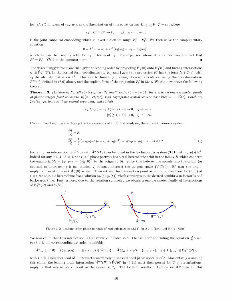
Proof. We begin by overlaying the two versions of (3.7) and studying the non-autonomous system

dq

dζ= p,

dp

dζ=

1

4

(−sgn(−ζ)q − cp+ 3q|q|2

)+ γ(2ip+ γq), (p, q) ∈ C2. (3.11)

For γ = 0, an intersection of W sr (0) with W cu

l (P0) can be found in the leading order system (3.11) with (q, p) ∈ R2.

Indeed for any 0 < 4− c 1, the ζ < 0 phase portrait has a real heteroclinic orbit in the family H which connects

the equilibria P0 = (q0, p0) := ( 1√3, 0)T to the origin (0, 0). Since this heteroclinic spirals into the origin (as

opposed to approaching it monotonically) it must intersect the tangent space T0Wsr (0) ∩ R2 near the origin,

implying it must intersect W sr (0) as well. Then setting this intersection point as an initial condition for (3.11) at

ζ = 0 we obtain a heteroclinic front solution (q∗(ξ), p∗(ξ)) which converges to the desired equilibria in forwards and

backwards time. Furthermore, due to the rotation symmetry we obtain a one-parameter family of intersections

of W cul (P) and W s

r (0).

p

q

Wrs(0)~

Wlcu(P0)~

P0

p

q

Wrs(0)~

Wlcu(P0)~

P0

Figure 3.2: Leading order phase portrait of real subspace in (3.11) for c > 4 (left) and c . 4 (right).

We now claim that this intersection is transversely unfolded in γ. That is, after appending the equation ddζγ = 0

to (3.11), the corresponding extended manifolds

W sr,ext(I × 0) = (γ, (p, q)) : γ ∈ I, (p, q) ∈ W s

r (0), W cul,ext(I × P) = (γ, (p, q)) : γ ∈ I, (p, q) ∈ W cu

l (P),

with I ⊂ R a neighborhood of 0, intersect transversely in the extended phase space R×C2. Momentarily assuming

this claim, the leading order intersection W cul (P) ∩ W s

r (0) in (3.11) must then persist for O(ε)-perturbations,

implying that intersections persist in the system (3.7). The foliation results of Proposition 3.2 then lift this

16

intersection to the full dynamics, implying that W sr (0) and W cu

l (P) intersect, from which we conclude the existence

of a planar trigger front solution W ∗(x, ξ) of (3.2), where once again W ∗(x, 0) is set to be at the intersection

point. To then obtain the 2π/ω-time-periodic solutions u∗ε (ξ, t), we simply set

u∗ε (ξ, t) = W ∗ε (ξ + ct, ξ), ω = ck.

Hence it only remains to prove the extended transversality claim. We prove this by using a Melnikov type

calculation to show that as γ is varied from 0 the invariant manifolds W cul (P) and W s

r (0) split with non-zero

speed.

First, we decompose (3.11) into real and imaginary variables q = qr + iqi, p = pr + ipi,

qr = pr,

pr = −1

4(µ(ξ)qr + cpr − 3qr(q

2r + q2

i ))− 2γpi,

qi = pi

pi = −1

4(µ(ξ)qi + cpi − 3qi(q

2r + q2

i ))− 2γpr, (3.12)

For short-hand we denote this system as Uζ = F (ξ, U ; c, γ) with U ∈ R4. First note that the heteroclinic front,

U∗(ζ) = (q∗(ζ), p∗(ζ), 0, 0)T found above in (3.11) for γ = 0, lies in the real subspace qi = pi = 0. We wish to

study how the invariant manifolds vary in γ near U∗(0) so we study the variational equation about U∗,

Vζ = A(ζ)V +G(ζ, V ; c, γ), (3.13)

A(ζ) = DUF (ζ, U∗(ζ); c, 0), G(ζ, V ; c, γ) = F (ζ, U∗(ζ) + V ; c, γ)− F (ζ, U∗(ζ); c, 0)−DUF (ζ, U∗(ζ); c, 0)V.

It then readily follows that the linear variational equation Vζ = A(ζ)V possesses exponential dichotomies Φs/ur (ζ, s)

for ζ, s > 0 and Φcu/ssl (ζ, s) for ζ, s < 0, with decay properties determined by the linearizations about the

asymptotic equilibria; see [33, 32] for a precise definition. The corresponding subspaces satisfy

Es/ur (ζ) := RgΦs/u

r (ζ, ζ), Es/ur (ζ) = TU∗(ζ)W

s/ur (0), ζ ≥ 0,

Ess/cul (ζ) := RgΦ

ss/cul (ζ, ζ) Ess/cu

r (ζ) = TU∗(ζ)Wss/cul (P0), ζ ≤ 0.

Furthermore, in a neighborhood of U∗(0), the invariant manifolds can be described by the sets

W cul (P0) = U∗(0) + vl + hcu

l (vl, γ) | hcul : Ecu

l (0)× R→ Essl (0),

W sr (0) := U∗(0) + vr + hs

r(vr, γ) | hsr : Es

r(0)× R→ Eur (0).

Then since there exists a one parameter family of intersections R(θ)U∗(0), where R(θ) is the real matrix

defined by the complex rotation (q, p) 7→ eiθ(q, p) in the basis qr, pr, qi, pi, we have dimR4Esr(0) ∩ Ecu

l (0) = 1,

and thus codimR4 Esr(0) + Ecu

l (0) = 1. Then using the fact that ∂θR(0)U∗(0) = (0, 0,−q∗(0),−p∗(0))T , an explicit

calculation gives that the vector ψ0 := (0, 0,−p∗(0), q∗(0))T satisfies

spanψ0 =[Es

r(0) + Ecul (0)

]⊥.

We then define a splitting distance for these invariant manifolds in a neighborhood of U∗(0),

S(γ, vl, vr) =⟨ψ0, h

cul (vl; γ)− hs

r(vr, γ)⟩R4,

for vr/l in some small neighborhood of zero, where here 〈·, ·〉R4 denotes the regular inner product in R4. Using the

variation of constants formula for the invariant manifolds we find

∂

∂γS(0, 0, 0) =

⟨ψ0, h

cul (0; 0)− hs

r(0; 0)⟩R4

=

⟨ψ0,

∫ 0

−∞Φss

l (0, ζ)∂γGdζ −∫ 0

∞Φu

r (0, ζ)∂γGdζ

⟩R4

, (3.14)

where

∂γG =∂

∂γG(0, c, 0) = (0,−2p∗(0), 0, 2p∗(0))T .

17

We then decompose this inner product and analyze each term separately. We first find∫ 0

∞

⟨ψ0,Φ

ur (0, ζ)∂γGdζ

⟩R4< 0,

by approximating Φur (0, ζ) by the linear flow of the asymptotic linearization about U = 0. We next find∫ 0

−∞

⟨ψ0,Φ

ssl (0, ζ)∂γG

⟩R4dζ > 0,

using a phase-plane analysis of the linearized flow about U∗(ζ) in qi, pi and the invariance of the real and

imaginary subspaces under the flow for γ = 0. We therefore have

∂

∂γS(0, 0, 0) > 0.

From this we conclude that in a neighborhood of U∗(0) the invariant manifolds W cur (P0) and W s

r (0) split for γ 6= 0

and thus are transversely unfolded in γ. This completes the proof of the theorem.

Using the transversality obtained in the above proof we can then prove genericity of the front u∗ε .

Proposition 3.3 (Genericity). The trigger front u∗ε is non-degenerate in the sense of Definition 1.1. That is the

linearization L about such a front has an algebraically simple Floquet exponent at λ = 0 when considered on the

exponentially weighted space L2η(R× T) for η > 0, small.

Proof. This result can be obtained by viewing the front as a heteroclinic orbit in a ξ-spatial dynamics

formulation. Given the extended transversality found in Theorem 3 above, and the spectral stability of the

asymptotic states u ≡ 0 and up (see [23]), one can use perturbation arguments in ε (see [31] or [11] for example)

to observe that the invariant manifolds of the asymptotic states W cul (up) and W s

r (0) in this spatial dynamics

formulation are transversely unfolded near u∗ε in the parameter ω. Then the approach of [33] can be used, viewing

u∗ε as a “transverse transmission” defect, to conclude algebraic simplicity of the zero eigenvalue.

Combining the results of Theorem 3 and Proposition 3.3 we obtain the existence of a planar trigger front in the

Swift-Hohenberg equation at onset satisfying the necessary hypotheses for Theorem 1. Hence we can conclude

the existence of obliquely striped trigger fronts in (1.3) at onset.

4 Applications and discussion

We discuss our results with possible extensions, and mention several applications.

Summary of results. We established existence of coherent structures that create striped patterns at a small

oblique angle to a quenching line, in the prototypical model of the Swift-Hohenberg equation. Technically, the

result is a singular perturbation result in the presence of continuous spectrum, perturbing from coherent pattern-

forming fronts that create stripes parallel to the quenching line. In the second part of this paper, we establish the

existence of these primary pattern-forming fronts.

Extending in parameter space. Ignoring the dependence on the parameter µ, our results establish exis-

tence for speeds 0 < c < clin and 0 < ky < ky(c). In a different direction, one could strive to establish existence

for ky 6= 0, 0 < c < cmax(ky). As in the case of stripe formation parallel to the quenching line, one expects the

maximal speed to be determined by a linear spreading speed, cmax(ky) = clin(ky), that is, the speeds at which

disturbances spread by means of pulled invasion fronts [38] when modulated in the transverse direction. It turns

out that for isotropic systems, such transversely modulated invasion speeds are always slower than non-modulated

invasion, clin(ky) < clin(0) for all ky 6= 0; [17, §7]. We therefore expect that, proving existence of transversely

modulated invasion fronts together with a gluing result as in [14] would give existence of oblique fronts up to

cmax(ky) = clin(ky), for a rather general class of pattern-forming equations. The fact that oblique fronts exist up

to a maximal speed slower than the maximal speed of parallel fronts then explains the fact that, across many

18

experiments from reaction-diffusion settings to phase separation processes, one observes stripes parallel to the

quenching line at large speeds.

For small speeds, at finite µ, wavenumber selection turns out to be quite intricate [13], and extensions to nonzero

ky appear to be difficult. Beyond small angles, ky ∼ 0, one can still attempt to construct stripe-forming fronts

for small µ, using the approach from Section 3 and more generally spatial dynamics and normal forms as in [36].

We expect more intricate behavior when ky approaches the zigzag-critical wavenumber, at which point we expect

kx ∼ 0. It would clearly be interesting to establish existence and non-existence of solutions globally in the space

of wavenumbers kx, ky and speeds c.

Stability, modulation, and selection. Beyond existence of solutions, the next natural question would be

concerned with their stability. One would expect linear stability of the waves, based on the approximation by a

monotone solution in the triggered Ginzburg-Landau amplitude equation. Having established spectral stability

in such a perturbative fashion, one expects nonlinear diffusive stability from results for coherent structures as

in [11]. A difficulty occurs, however, when considering perturbations that are not co-periodic in the y-direction.

Already linear stability of the selected stripe solution with respect to such perturbations is not evident. As

demonstrated in [35], relying on [13], parallel stripes selected by slowly moving triggers are unstable against

transverse perturbations due to a zigzag instability. The instability may however be propagating at a slower

speed than the quenching, such that unstable patterns can be observed in a large region in the wake of the

quenching line. Similar formation of unstable, or merely metastable patterns in the wake of the quenching line

has been observed in phase separation processes; see [25] and references therein. It is worth noticing that our

perturbation analysis is insensitive to these instabilities, as the main non-degeneracy assumption only relies on

co-periodic stability of the periodic patterns. Other instabilities are non-resonant with the mode of propagation

and therefore do not change the Fredholm index; see [15, §4] for the notion of non-resonance in this context.

On the other hand, the fact that stripe formation occurs for a family of wavenumbers ky ∼ 0 raises the question of

possible interaction of wavenumbers, modulating an initial condition slowly in the transverse direction along stripe-

forming fronts with wavenumber ky(εy). Focusing on the dynamics at the interfacial line and neglecting the farfield

patterns, one then observes temporal oscillations that are slowly modulated in y and expects dynamics for the

wavenumber ky given by Burgers’ equation [4]. It would be interesting to understand if and how these interfacial

dynamics interact with the far-field striped patterns. Beyond ky ∼ 0, one observes more complicated dynamics,

such as interaction between stripes formed parallel to the interface in y > 0, say, and stripes perpendicular to

the interface in y < 0, say, creating permanent grain boundaries between different stripe orientation in their wake

[22, 36].

Experiments. We briefly report on experiments exhibiting the parallel and oblique stripe formation. Consid-

ering the Swift-Hohenberg equation as a prototypical model for Turing instabilities leading to striped phases, the

most relevant recent experiments have been performed using a light-sensing reaction-diffusion system, striving to

illustrate the effect of domain growth on the formation of Turing patterns [24]. More specifically, the authors

studied a CDIMA reaction in a gel in which high intensity light suppresses a spatial Turing instability. They found

that by moving an opaque mask, which blocked the light, across the surface of the gel at different speeds, different

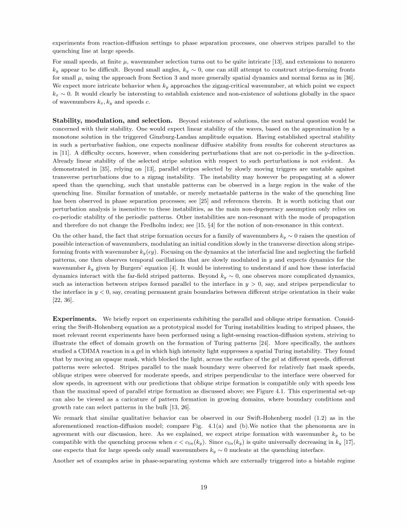
patterns were selected. Stripes parallel to the mask boundary were observed for relatively fast mask speeds,

oblique stripes were observed for moderate speeds, and stripes perpendicular to the interface were observed for

slow speeds, in agreement with our predictions that oblique stripe formation is compatible only with speeds less

than the maximal speed of parallel stripe formation as discussed above; see Figure 4.1. This experimental set-up

can also be viewed as a caricature of pattern formation in growing domains, where boundary conditions and

growth rate can select patterns in the bulk [13, 26].

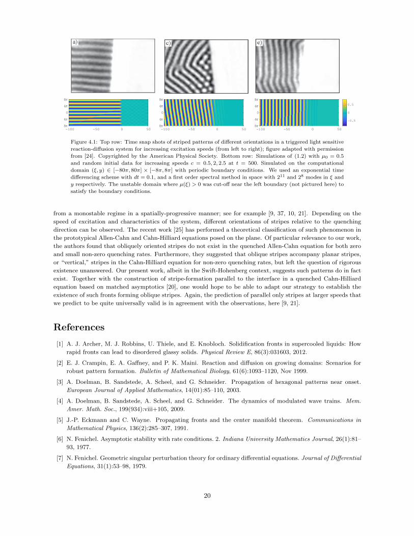
We remark that similar qualitative behavior can be observed in our Swift-Hohenberg model (1.2) as in the

aforementioned reaction-diffusion model; compare Fig. 4.1(a) and (b).We notice that the phenomena are in

agreement with our discussion, here. As we explained, we expect stripe formation with wavenumber ky to be

compatible with the quenching process when c < clin(ky). Since clin(ky) is quite universally decreasing in ky [17],

one expects that for large speeds only small wavenumbers ky ∼ 0 nucleate at the quenching interface.

Another set of examples arise in phase-separating systems which are externally triggered into a bistable regime

19

-100 -50 0 50

8

4

0

4

8

-0.5

0

0.5

-100 -50 0 50

8

4

0

4

8

-0.5

0

0.5

-100 -50 0 50

8

4

0

4

8

-0.5

0

0.5

Figure 4.1: Top row: Time snap shots of striped patterns of different orientations in a triggered light sensitive

reaction-diffusion system for increasing excitation speeds (from left to right); figure adapted with permission

from [24]. Copyrighted by the American Physical Society. Bottom row: Simulations of (1.2) with µ0 = 0.5

and random initial data for increasing speeds c = 0.5, 2, 2.5 at t = 500. Simulated on the computational

domain (ξ, y) ∈ [−80π, 80π] × [−8π, 8π] with periodic boundary conditions. We used an exponential time

differencing scheme with dt = 0.1, and a first order spectral method in space with 211 and 28 modes in ξ and

y respectively. The unstable domain where µ(ξ) > 0 was cut-off near the left boundary (not pictured here) to

satisfy the boundary conditions.

from a monostable regime in a spatially-progressive manner; see for example [9, 37, 10, 21]. Depending on the

speed of excitation and characteristics of the system, different orientations of stripes relative to the quenching

direction can be observed. The recent work [25] has performed a theoretical classification of such phenomenon in

the prototypical Allen-Cahn and Cahn-Hilliard equations posed on the plane. Of particular relevance to our work,

the authors found that obliquely oriented stripes do not exist in the quenched Allen-Cahn equation for both zero

and small non-zero quenching rates. Furthermore, they suggested that oblique stripes accompany planar stripes,

or “vertical,” stripes in the Cahn-Hilliard equation for non-zero quenching rates, but left the question of rigorous

existence unanswered. Our present work, albeit in the Swift-Hohenberg context, suggests such patterns do in fact

exist. Together with the construction of stripe-formation parallel to the interface in a quenched Cahn-Hilliard

equation based on matched asymptotics [20], one would hope to be able to adapt our strategy to establish the

existence of such fronts forming oblique stripes. Again, the prediction of parallel only stripes at larger speeds that

we predict to be quite universally valid is in agreement with the observations, here [9, 21].

References

[1] A. J. Archer, M. J. Robbins, U. Thiele, and E. Knobloch. Solidification fronts in supercooled liquids: How

rapid fronts can lead to disordered glassy solids. Physical Review E, 86(3):031603, 2012.

[2] E. J. Crampin, E. A. Gaffney, and P. K. Maini. Reaction and diffusion on growing domains: Scenarios for

robust pattern formation. Bulletin of Mathematical Biology, 61(6):1093–1120, Nov 1999.

[3] A. Doelman, B. Sandstede, A. Scheel, and G. Schneider. Propagation of hexagonal patterns near onset.

European Journal of Applied Mathematics, 14(01):85–110, 2003.

[4] A. Doelman, B. Sandstede, A. Scheel, and G. Schneider. The dynamics of modulated wave trains. Mem.

Amer. Math. Soc., 199(934):viii+105, 2009.

[5] J.-P. Eckmann and C. Wayne. Propagating fronts and the center manifold theorem. Communications in

Mathematical Physics, 136(2):285–307, 1991.

[6] N. Fenichel. Asymptotic stability with rate conditions. 2. Indiana University Mathematics Journal, 26(1):81–

93, 1977.

[7] N. Fenichel. Geometric singular perturbation theory for ordinary differential equations. Journal of Differential

Equations, 31(1):53–98, 1979.

20

[8] B. Fiedler and A. Scheel. Spatio-temporal dynamics of reaction-diffusion patterns. In Trends in nonlinear

analysis, pages 23–152. Springer, Berlin, 2003.

[9] E. Foard and A. Wagner. Survey of morphologies formed in the wake of an enslaved phase-separation front

in two dimensions. Physical Review E, 85(1):011501, 2012.

[10] H. Furukawa. Phase separation by directional quenching and morphological transition. Physica A: Statistical

Mechanics and its Applications, 180(1):128 – 155, 1992.

[11] T. Gallay, G. Schneider, and H. Uecker. Stable transport of information near essentially unstable localized

structures. Discrete Contin. Dyn. Syst. Ser. B, 4(2):349–390, 2004.

[12] K. Glasner. Hexagonal phase ordering in strongly segregated copolymer films. Phys. Rev. E, 92:042602, Oct

2015.

[13] R. Goh, R. Beekie, D. Matthias, J. Nunley, and A. Scheel. Universal wave-number selection laws in apical

growth. Phys. Rev. E, 94:022219, Aug 2016.

[14] R. Goh and A. Scheel. Triggered fronts in the complex Ginzburg Landau equation. Journal of Nonlinear

Science, 24(1):117–144, 2014.

[15] R. N. Goh, S. Mesuro, and A. Scheel. Spatial wavenumber selection in recurrent precipitation. SIAM J.

Appl. Dyn. Syst., 10(1):360–402, 2011.

[16] M. Haragus-Courcelle and G. Schneider. Bifurcating fronts for the Taylor–Couette problem in infinite cylin-

ders. Zeitschrift fur angewandte Mathematik und Physik, 50(1):120–151, 1999.

[17] M. Holzer and A. Scheel. Criteria for pointwise growth and their role in invasion processes. Journal of

Nonlinear Science, 24(4):661–709, 2014.

[18] T. Kato. Perturbation theory for linear operators, volume 132. Springer Science & Business Media, 1966.

[19] M. H. Kopf and U. Thiele. Emergence of the bifurcation structure of a Langmuir–Blodgett transfer model.

Nonlinearity, 27(11):2711, 2014.

[20] A. Krekhov. Formation of regular structures in the process of phase separation. Phys. Rev. E, 79:035302,

Mar 2009.

[21] R. Kurita. Control of pattern formation during phase separation initiated by a propagated trigger. Scientific

Reports, 7(1):6912, 2017.

[22] D. J. B. Lloyd and A. Scheel. Continuation and bifurcation of grain boundaries in the Swift-Hohenberg

equation. SIAM J. Appl. Dyn. Syst., 16(1):252–293, 2017.

[23] A. Mielke. Instability and stability of rolls in the Swift-Hohenberg equation. Comm. Math. Phys., 189(3):829–

853, 1997.

[24] D. G. Mıguez, M. Dolnik, A. P. Munuzuri, and L. Kramer. Effect of axial growth on Turing pattern formation.

Physical Review Letters, 96(4):048304, 2006.

[25] R. Monteiro and A. Scheel. Phase separation patterns from directional quenching. Journal of Nonlinear

Science, Feb 2017.

[26] D. Morrissey and A. Scheel. Characterizing the effect of boundary conditions on striped phases. SIAM

Journal on Applied Dynamical Systems, 14(3):1387–1417, 2015.

[27] M. Pennybacker and A. C. Newell. Phyllotaxis, pushed pattern-forming fronts, and optimal packing. Physical

Review Letters, 110(24):248104, 2013.

[28] J. D. Rademacher and A. Scheel. The saddle-node of nearly homogeneous wave trains in reaction–diffusion

systems. Journal of Dynamics and Differential Equations, 19(2):479–496, 2007.

[29] E. Risler. Travelling waves and dispersion relation in the spatial unfolding of a periodic orbit. C. R. Math.

Acad. Sci. Paris, 334(9):833–838, 2002.

[30] M. J. Robbins, A. J. Archer, U. Thiele, and E. Knobloch. Modeling the structure of liquids and crystals

using one-and two-component modified phase-field crystal models. Physical Review E, 85(6):061408, 2012.

[31] B. Sandstede and A. Scheel. Essential instability of pulses and bifurcations to modulated travelling waves.

Proceedings of the Royal Society of Edinburgh-A-Mathematics, 129(6):1263–1290, 1999.

21

[32] B. Sandstede and A. Scheel. On the structure of spectra of modulated travelling waves. Mathematische

Nachrichten, 232(1):39–93, 2001.

[33] B. Sandstede and A. Scheel. Defects in oscillatory media: toward a classification. SIAM Journal on Applied

Dynamical Systems, 3(1):1–68, 2004.

[34] B. Sandstede and A. Scheel. Relative Morse indices, fredholm indices, and group velocities. Discrete and

Continuous Dynamical Systems A, pages 139–158, 2008.

[35] A. Scheel and J. Weinburd. Wavenumber selection in a quenched Swift-Hohenberg equation. Preprint, 2017.

[36] A. Scheel and Q. Wu. Small-amplitude grain boundaries of arbitrary angle in the Swift-Hohenberg equation.

ZAMM Z. Angew. Math. Mech., 94(3):203–232, 2014.

[37] S. Thomas, I. Lagzi, F. Molnar Jr, and Z. Racz. Probability of the emergence of helical precipitation patterns

in the wake of reaction-diffusion fronts. Physical Review Letters, 110(7):078303, 2013.

[38] W. Van Saarloos. Front propagation into unstable states. Physics Reports, 386(2):29–222, 2003.

R. Goh (Corresponding author), Department of Mathematics and Statistics, Boston University, 111 Cummington

Mall, Boston, MA 02215

E-mail address, R. Goh: rgoh@bu.edu

A. Scheel, School of Mathematics, University of Minnesota, 206 Church St. SE, Minneapolis, MN 55455

E-mail address, A. Scheel: scheel@umn.edu

22