pattern classification basic principles and tools

Pattern classification

Basic principles and tools

Pattern Classification, Chapter 1

2

Summary

• Why a lecture on pattern recognition?

• Introduction to Pattern Recognition (Duda - Sections 1.1-1.6)

• An example of unsupervised learning: PCA

• Tools


3

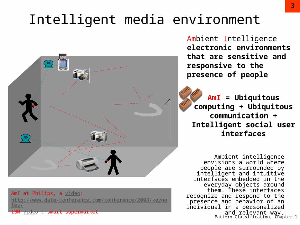
Intelligent media environmentAmbient Intelligenceelectronic environmentsthat are sensitive and responsive to the presence of people

AmI = Ubiquitous computing + Ubiquitous

communication + Intelligent social user

interfaces

Ambient intelligence envisions a world where people are

surrounded by intelligent and intuitive interfaces embedded in

the everyday objects around them. These interfaces recognize and respond to the presence and

behavior of an individual in a personalized and relevant way.

AmI at Philips, a video:http://www.date-conference.com/conference/2003/keynotes/IBM video : smart supermarket

http://www.date-conference.com/conference/2003/keynotes/


4

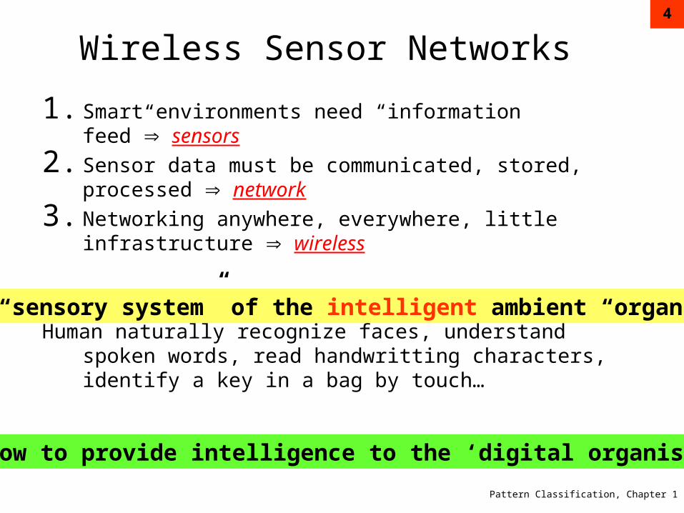
Wireless Sensor Networks

1. Smart environments need “information feed” sensors

2. Sensor data must be communicated, stored, processed network

3. Networking anywhere, everywhere, little infrastructure wireless

Human naturally recognize faces, understand spoken words, read handwritting characters, identify a key in a bag by touch…

The “sensory system” of the intelligent ambient “organism”

How to provide intelligence to the ‘digital organism’?


5

What is pattern recognition?

• A pattern is an object, process or event that can be given a name.

• A pattern class (or category) is a set of patterns sharing common attributes and usually originating from the same source.

• During recognition (or classification) given objects are assigned to prescribed classes.

• A classifier is a machine which performs classification.

“The assignment of a physical object or event to one of several pre-specified categories” -- Duda & Hart


6

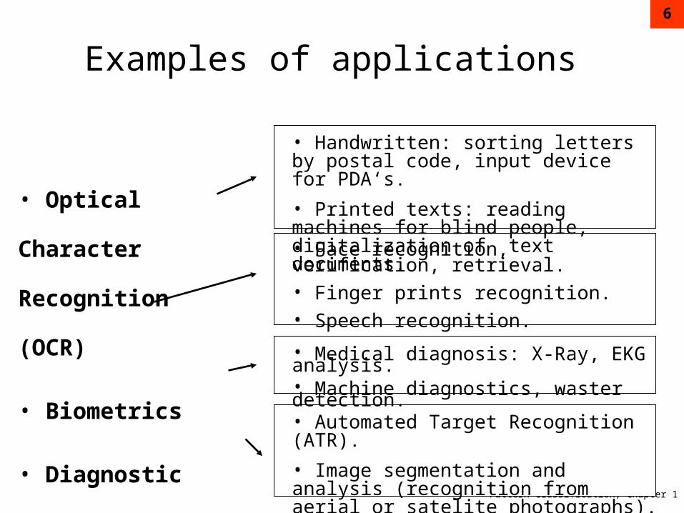
Examples of applications

• Optical Character

Recognition (OCR)

• Biometrics

• Diagnostic systems

• Military applications

• Handwritten: sorting letters by postal code, input device for PDA‘s.

• Printed texts: reading machines for blind people, digitalization of text documents.

• Face recognition, verification, retrieval. • Finger prints recognition.• Speech recognition.

• Medical diagnosis: X-Ray, EKG analysis.• Machine diagnostics, waster detection.

• Automated Target Recognition (ATR).

• Image segmentation and analysis (recognition from aerial or satelite photographs).


7

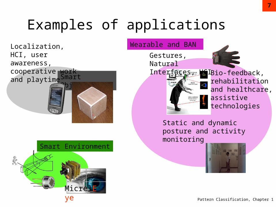
Examples of applications

Smart Objects

Wearable and BAN

Smart Environment

Gestures, Natural Interfaces, HCI

Localization, HCI, user awareness, cooperative work and playtime Bio-feedback,

rehabilitation and healthcare, assistive technologies

Static and dynamic posture and activity monitoring

MicrelEye


8

Design space

• The design space is wide… two examples:• Seq. of static posture:

• Threshold based algorithm, network star topology:

• Can be embedded in microcontroller

• Can be distributed among nodes

• More nodes (to understand complex postures) means problems in terms of: scalability, wearability, real-time loss, etc…

• Activity recognition (Gait): one sensor• SVM based algorithm, one sensor

• Extreme wearability

• Need computational power

• Can understand more complex activity


9

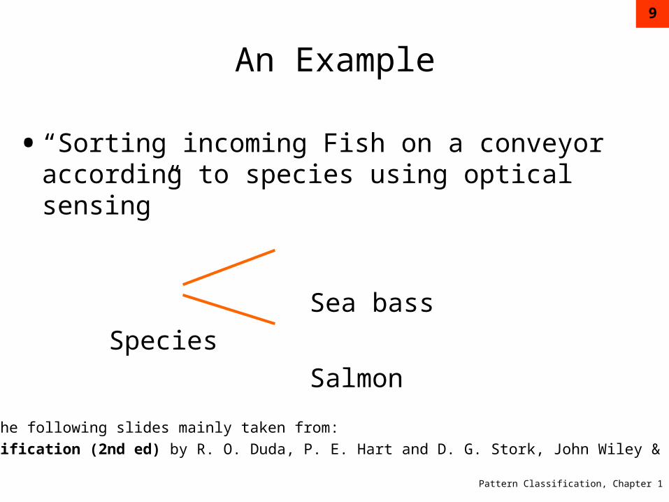
An Example

• “Sorting incoming Fish on a conveyor according to species using optical sensing”

Sea bass

Species

Salmon

Material of the following slides mainly taken from:

Pattern Classification (2nd ed) by R. O. Duda, P. E. Hart and D. G. Stork, John Wiley & Sons, 2000


10

• Problem Analysis

• Set up a camera and take some sample images to extract features

• Length

• Lightness

• Width

• Number and shape of fins

• Position of the mouth, etc…

• This is the set of all suggested features to explore for use in our classifier!


11

• Preprocessing

• Use a segmentation operation to isolate fishes from one another and from the background

• Information from a single fish is sent to a feature extractor whose purpose is to reduce the data by measuring certain features

• The features are passed to a classifier


12


13

• Classification

• Select the length of the fish as a possible feature for discrimination


14

The length is a poor feature alone!

Select the lightness as a possible feature.


15

• Threshold decision boundary and cost relationship

• Move our decision boundary toward smaller values of lightness in order to minimize the cost (reduce the number of sea bass that are classified salmon!)

Task of decision theory


16

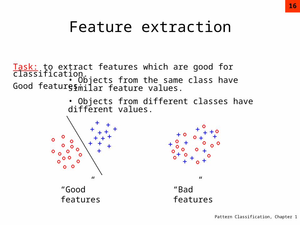
Feature extraction

Task: to extract features which are good for classification.

Good features: • Objects from the same class have similar feature values.

• Objects from different classes have different values.

“Good” features “Bad” features


17

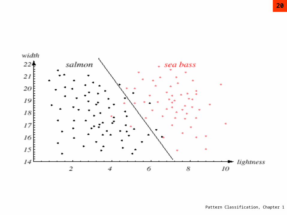
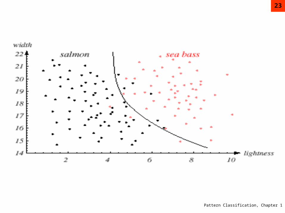
• Adopt the lightness and add the width of the fish

Fish xT = [x1, x2]

Lightness Width

Feature vector


18

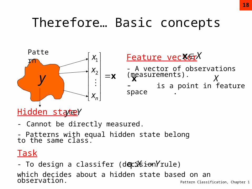
Therefore… Basic concepts

y x

nx

x

x

2

1 Feature vector

- A vector of observations (measurements). - is a point in feature space .

Hidden state

- Cannot be directly measured.

- Patterns with equal hidden state belong to the same class.

Xx

x X

Yy

Task- To design a classifer (decision rule)

which decides about a hidden state based on an observation.

YX :q

Pattern


19

In our case…

x

2

1

x

x

lightness

width

Task: fish recognition.

The set of hidden state is

The feature space is

},{ JHY2X

Training examples

)},(),...,,{( 11 ll yy xx

1x

2x

Jy

Hy Linear classifier:

0)(

0)()q(

bifJ

bifH

xw

xwx

0)( bxw

Sea bassSalmon


20


21

• We might add other features that are not correlated with the ones we already have. A precaution should be taken not to reduce the performance by adding such “noisy features”

• Ideally, the best decision boundary should be the one which provides an optimal performance such as:


22

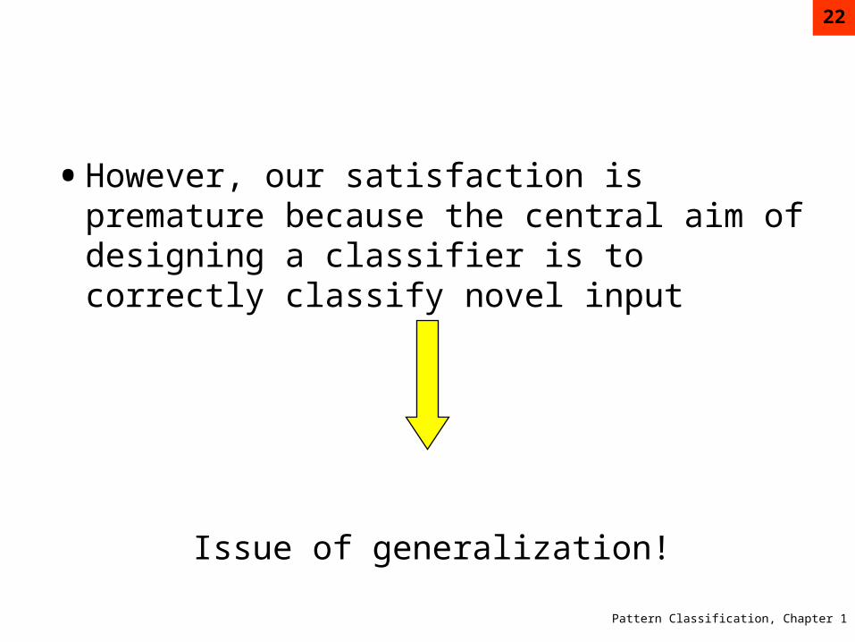
• However, our satisfaction is premature because the central aim of designing a classifier is to correctly classify novel input

Issue of generalization!


23


24

Overfitting and underfitting

Problem:

underfitting overfittinggood fit


25

Components of PR system

Sensors and preprocessing

Feature extraction

Classifier

Classassignment

• Sensors and preprocessing (segmentation / windowing)• A feature extraction aims to create discriminative features good for classification.• A classifier.• A teacher provides information about hidden state -- supervised learning.• A learning algorithm sets PR from training examples.

Learning algorithmTeacher

Pattern


26

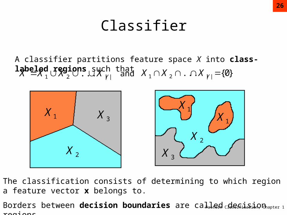
Classifier

A classifier partitions feature space X into class-labeled regions such that

||21 ... YXXXX }0{... ||21 YXXXand

1X 3X

2X

1X1X

2X

3X

The classification consists of determining to which region a feature vector x belongs to.

Borders between decision boundaries are called decision regions.


27

Representation of classifier

A classifier is typically represented as a set of discriminant functions

||,...,1,:)(f YX ii x

The classifier assigns a feature vector x to the i-the class if )(f)(f xx ji ij

)(f1 x

)(f2 x

)(f || xY

maxx y

Feature vector

Discriminant function

Class identifier


28

Post-processing and evaluation

• Voting

• Costs and Risks

• Computational complexity (differentiating between learning and classifying)


29

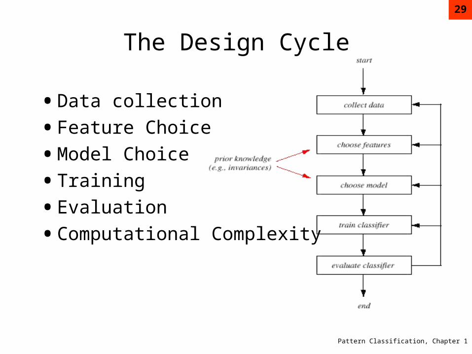
The Design Cycle

• Data collection

• Feature Choice

• Model Choice

• Training

• Evaluation

• Computational Complexity


30

• Data Collection• How do we know when we have collected an

adequately large and representative set of examples for training and testing the system?

• Feature Choice• Depends on the characteristics of the problem

domain. Simple to extract, invariant to irrelevant transformation insensitive to noise.

• Model Choice• Unsatisfied with the performance of our fish

classifier and want to jump to another class of model


31

• Training• Use data to determine the classifier. Many different

procedures for training classifiers and choosing models

• Evaluation• Measure the error rate (or performance and switch

from one set of features to another one

• Computational Complexity• What is the trade-off between computational ease

and performance?

• (How an algorithm scales as a function of the number of features, patterns or categories?)


32

Learning and Adaptation

• Supervised learning

• A teacher provides a category label or cost for each pattern in the training set

• Unsupervised learning

• The system forms clusters or “natural groupings” of the input patterns


33

Unsupervised learning: PCA

• Principal Component Analysis

• Used abundantly because it is a method for extracting relevant information from confusing datasets

• It is Simple and Non parametric

• Can be used to reduce a complex data set to a lower dimension, revealing hidden simplified structures

• Starting point - we are experimenter: phenomenon to measures, but data appears clouded, unclear, redundant


34

Unsupervised learning: PCA as example

• The Toy Example: motion of the ideal springA ball of mass m attached to a massless, frictionless spring. The ball is released a small distance

away from equilibrium it oscillates indef. along x at a set freq about its equilibrium We are ignorant we don’t know how many axes and

dimensions to measure

We decide to use:- 3 cameras, not orthogonal

- each camera records at 200Hz an image of the two-dim position of rthe ball (a projection)

- we chose three axes {a,b,c}


35

The Toy Example – con’t

• how do we get from this data set to a simple equation of x?

• One goal of PCA is to compute the most meaningful basis to re-express a noisy data set.

• Goal in our example: “the dynamics are along the x-axis.” x - the unit basis vector along the x-axis - is the important dimension.

• Our data set is at each time:

Where each camera contributes a 2-dimensional projection of the ball’s position to the entire vector X

If we record the ball’s position for 10 minutes at 120 Hz, then we have recorded 10x60x120 = 72000 of these vectors.


36

Change of Basis• Each sample X is an m-dimensional vector, where m

is the number of measurements types (e.g. 6) every samples is a vector lying in an m-dim vector space spanned by an orthonormal basis B and can be expressed as a lin. comb. of bi

• Exist B’, which is lin comb of B, that best re-expresses our data set?

• Linearity assumption• restrict potential basis

• formalize implicit assumption of dataset continuity

• PCA limited to re-express the data as a linear combination of its basis vector


37

• X be the original data set (columns =samples in t)

• X is m x n (m=6, n=72000)

• Y is m x n related to X by P

PX=Y 1. P is a matrix that transforms X in Y

2. P is geometrically a rotation and stretch between X, Y

3. And…The rows of P, {p1, . . . , pm}, are a set of new basis vectors for expressing the columns of X.

• jth coeff of yi is a projection on the jth row of P

• Therefore the rows of P are a new set of basis vectors for columns of X


38

Variance and the goal

• Rows of P principal component of X• What is the best way to re-express X?

• What is a good choice for P?

• What does“best express” the data mean?

• Decipher ‘garbled’ data. In a linear system “garbled” refers to:

• noise,

• rotation and

• redundancy.


39

A. Noise and RotationNoise is measured relative to the measurement. A common

measure is the signal-to-noise ratio (SNR), or a ratio of variances σ2

SNR (>> 1) precision data, low SNR noise contaminated dataSimulated data of (xA, yA) for camera A.

• SNR measures how “fat” the cloud is • We assume that directions with largest variances in our measurement vector space contain the dynamics of interest.

Maximizing the variance (and by assumption the SNR ) corresponds to finding the appropriate rotation of the naive basis.


40• This intuition corresponds to finding the direction p in Figure 2b. How do we find p* In the 2-dimensional case of Figure 2a, p falls along the direction of the best-fit line for the data cloud. Thus, rotating the naive basis to lie parallel to p would reveal the direction of motion of the spring for the 2-D case.


41

B. Redundancy

• On the other extreme, Figure 3c depicts highly correlated recordings.

• Clearly in panel (c) it would be more meaningful to just have recorded a single variable, not both.

• Indeed, this is the very idea behind dimensional reduction.

• Possible plots between two arbitrary measurement types r1 and r2.

(a) no apparent relationship = r1 is entirely uncorrelated with r2. r1 and r2 are statistically independent.


42

Covariance matrix

• Generalizing to higher dimensionality

• Two sets of measurements (zero-mean)

• The variances are:

• And covariance

• The covariance measures the degree of the linear relationship between two variables. A large (small) value indicates high (low) redundancy.


43

• Generalizing to m vectors x1…xm we obtain a m x n matrix

• Each row of X corresponds to all measurements of a particular type (xi).

• Each column of X corresponds to a set of measurements from one particular trial

• Covariance matrix:


44

• CX is a square symmetric m x m matrix.

• The diagonal terms of CX are the variance of particular measurement types.

• The off-diagonal terms of CX are the covariance between measurement types.

• CX captures the correlations between all possible pairs of measurements. The correlation values reflect the noise and redundancy in our measurements.• In the diagonal terms, by assumption, large (small) values correspond

to interesting dynamics (or noise).

• In the off-diagonal terms large (small) values correspond to high (low) redundancy.

• Pretend we have the option of manipulating CX. We will suggestively define our manipulated covariance matrix CY. What features do we want to optimize in CY?


45

Diagonalize the Covariance Matrix

(1) to minimize redundancy, measured by covariance,

(2) maximize the signal, measured by variance.

CY must be diagonal

To do so PCA use the easiest way:

- PCA assumes P is an orthonormal matrix

- PCA assumes the directions with the largest variances the signals and the most “important” or principal

- P acts as a generalized rotation to align a basis with the maximally variant axis


46

1. Select a normalized direction in m-dimensional space along which the variance in X is maximized. Save this vector as p1.

2. Find another direction along which variance is maximized, however, because of the orthonormality condition, restrict the search to all directions perpendicular to all previous selected directions. Save this vector as p2

3. Repeat this procedure until m vectors are selected.

Y=PX and CY is diagonal


47

SOLVING PCATwo ways for the algebraic solution:

• EIGENVECTORS OF COVARIANCE

• A MORE GENERAL SOLUTION: SVD (singular value decomposition)

The first method corresponds for a given data set X to(1) Subtract the mean of each measurements type(2) Compute the eigenvectors of XXT (= obtain P)

More in general performing PCA is done by three steps1. Organize a data set as an m x n matrix, where m is the

number of measurement types and n is the number of trials.2. Subtract off the mean for each measurement type or row xi.3. Calculate the SVD or the eigenvectors of the covariance.


48

TOOLS and demonstration (30min)

– Commercial– Open-source• WEKA

http://www.cs.waikato.ac.nz/~ml/weka/index.html• YALE (now RapidMiner http://rapid-i.com/)• The R Project for Statistical Computing http://www.r-

project.org/• Pentaho – whole BI solutions.

http://www.pentaho.com/– Matlab

pattern classification basic principles and tools

Documents