pathfinding through urban traffic using dijkstra’s...

Makalah IF2091 Struktur Diskrit – Sem. I Tahun 2011/2012

Pathfinding through urban traffic using Dijkstra’s Algorithm

Tubagus Andhika Nugraha (13510007)

Program Studi Teknik Informatika Sekolah Teknik Elektro dan Informatika

Institut Teknologi Bandung, Jl. Ganesha 10 Bandung 40132, Indonesia [email protected]; [email protected]

Abstract—Getting from place to place is a problem for citizens of urban cities that worsens every day due to the inevitable increase in vehicle ownership leading to more traffic on roads and the impending traffic jams that come with them. Efficient urban travel requires a route that is not only short in terms of distance, but also takes less time by avoiding the worst traffic. This paper discusses how Dijkstra’s algorithm can be used to find the optimal path for travelling inside a city.

Index Terms—Dijkstra’s algorithm, graph theory,

pathfinding, traffic

I. INTRODUCTION

Citizens of Jakarta, the populous, metropolitan capital of Indonesia would describe living in the city as “getting old on the road”. Traffic jams have become an increasing problem for the citizens of not only Jakarta, but also other metropolitan cities in the world. As an example, analysts have predicted that by the year 2050, traffic in Jakarta will be congested up to the point of freezing entirely.

The traffic jam problem may be a problem that must be solved by politicians and city planners, but it may take more than a decade for any real major long-term change to materialize. Practically, citizens would benefit from just a way to navigate through city traffic and get home from work in an efficient manner. Doing so would have to take into account not just distance, but also traffic, as a factor in determining the most optimal route. Such a route can be generated automatically using computers.

The task of finding a route between two points is called pathfinding. Pathfinding in general is used in a lot of applications, from airplane routing to intelligent robots. Most applications of pathfinding utilize a branch of discrete mathematics called graph theory. The same idea can be applied to the traffic jam problem. We first represent the city map that includes our origin and destination points as a graph, then we calculate the optimal path based on that graph.

One of the most common ways of finding such an optimal path in graphs is using a graph search algorithm called Dijkstra’s algorithm. This paper shall discuss how Dijkstra’s algorithm can be applied in pathfinding through urban traffic.

II. THEORIES

A. City Maps A city map is a large-scale thematic map of a city (or

part of a city) created to enable the fastest possible orientation in an urban space. [1] A city map generally contains the city’s transport network, in the form of roads, highways, as well as railroads, tram networks, monorails and other forms of public transportation. Generally, roads are symbolized by lines with their thickness representing the size of the road, i.e. highways and artery roads are thicker than streets in residential areas. Likewise, crisscrossing lines represent intersections. Public transportation lines are generally represented with other forms of lines, but they are outside the context of this paper. Buildings and open green spaces are denoted as the spaces between roads.

In the context of this paper, three types of objects within city maps are of interest: buildings, roads and intersections. Buildings are used as start and end points for the traveller. Roads are used as the basis for the route,


because simply, cars can only travel through roads. Intersections split roads into sections of roads, which will be the unit of calculation, as we will see in Chapter III. Lengths of sections of roads can then be inferred from measuring the distance between intersections on the map and applying the appropriate scale.

Besides distance, we also need to take into account the amount of traffic going through a section of road. This data can be represented in many ways, but for this paper, we shall measure the traffic through a section of road in terms of the average speed of the cars travelling through the section of road. We shall measure such speed in kilometers per hour (km/h).

B. Graph Theory A graph is an abstract representation of a set of objects

where some pairs of the objects are connected by links. The interconnected objects are represented by mathematical abstractions called vertices, and the links that connect some pairs of vertices are called edges. Typically, a graph is depicted in diagrammatic form as a set of dots for the vertices, joined by lines or curves for the edges. [2]

There are multiple types of graphs, depending on how to categorize them. A graph may be undirected, that is, there is no distinction between the two vertices connected by an edge, or it may be directed from one vertex to another. An example of an undirected graph would be people shaking hands, where each person is represented by a vertex and their shaking hands represented by an edge. When two people shake hands, there is no distinction between the two, and thus, it is a symmetric act, therefore an undirected graph. A purchase at the market, however, would be asymmetric, as there would be a seller and a buyer. This is an example of a directed graph. Mixed graphs are graphs in which some edges are directed and some aren’t. Below is an example of a directed graph.

Another distinction among graphs is between weighted

and non-weighted graphs. In non-weighted graphs, there is no distinction between one edge and another in terms of significance. Every edge is considered equal; the only difference is the vertices they connect. In weighted graphs, however, numbers are assigned to each edge. These numbers may represent cost, distance, and

capacities, among others, depending on the problem at hand.

There are also simple graphs and multigraphs. In simple graphs, two vertices can only be connected by one edge, whereas in multiple graphs, multiple edges are allowed.

Besides edges and vertices, there are also other useful concepts in graph theory. One particular concept of use in this paper is paths. A path in a graph is a sequence of vertices such that from each of its vertices there is an edge to the next vertex in the sequence. A path may be infinite, but a finite path always has a first vertex, called its start vertex, and a last vertex, called its end vertex. Both of them are called terminal vertices of the path. The other vertices in the path are internal vertices. [3] In weighted graphs, the weight of a path is the sum of the weights of all the edges that the path consists of.

Applications in graph theory range from city planning to electronic circuit design, including, as this paper will show, pathfinding through urban traffic.

C. Dijkstra’s Algorithm As explained before, in weighted graphs, the weight of

a path can be calculated as the sum of the weights of the edges inside the path. Finding the shortest path between two vertices is called the shortest path problem. Several algorithms exist to solve different variations of the shortest path problem; of which one is Dijkstra’s algorithm.

Dijkstra’s algorithm was conceived by Dutch computer scientist Edsger Dijkstra in 1956 and published in 1959. For a given source vertex (node) in the graph, the algorithm finds the path with lowest cost (i.e. the shortest path) between that vertex and every other vertex. It can also be used for finding costs of shortest paths from a single vertex to a single destination vertex by stopping the algorithm once the shortest path to the destination vertex has been determined. [4]

The algorithm Let the node at which we are starting be called the

initial node. Let the distance of node Y be the distance from the initial node to node Y. Dijkstra’s algorithm will then run as follows:

1. Assign a tentative distance value to every node. Set it zero for the initial node, and infinity for every other node.

2. Mark all nodes as unvisited. Set the initial node as current. Create a set of the unvisited nodes and call it the unvisited set.

3. For the current node, consider all of its unvisited neighbors and calculate their tentative distances. For example, if the current node X is marked with a distance of 4 (from the initial node), and the edge connecting it with neighbor Y has length 3, then the distance to B will be 4+3=7. If this distance is less than the previously recorded distance, then overwrite that distance. Even though a neighbor

A

B

C D

E


has been examined, it is not marked as visited at this time, and it remains the unvisited set.

4. Once every neighbor of the current node has been considered, mark the current node as visited and remove it from the unvisited set. A visited node will never be checked again; its distance recorded now is final and minimal.

5. If the destination node has been marked as visited or if the smallest tentative distance among the nodes in the unvisited set is infinity, then the algorithm has finished.

6. Set the unvisited node marked with the smallest tentative distance as the next current node and go back to step 3 [4].

In pseudocode, Dijkstra’s algorithm can be described as follows:

function Dijkstra (G: Graph, S: Vertex) → real { G is a Graph with each edge E in the

form of (v1, v2) and vertices V. S is the source vertex. }

DECLARATIONS dist: array of real { array of distances

from the source to each vertex } prev: array of pointer to Vertex { array

of pointers to preceding vertices } i: integer { loop index } F: list of Vertex { finished vertices } U: list of Vertex { unfinished vertices } ALGORITHM { Init: set every distance to ∞ } iterate [0..(abs(G.V)–1)] dist[i] = ∞ prev[i] = Nil { end iterate } { The distance from the source to the

source is defined to be zero } dist[S] = 0 while (F is missing a vertex) do V ← the vertex in U with the shortest

path to S Insert(F, V) foreach edge of V as (v1, v2) if (dist[v1] + length(v1, v2) <

dist[v2]) then dist[v2] = dist[v1] +

length(v1, v2) prev[v2] = v1 { end if } { end foreach } { end while }

{ [5] } Dijkstra's original algorithm does not use a min-priority

queue and runs in O(|V|2). The idea of this algorithm is also given in (Leyzorek et al. 1957). The common implementation based on a min-priority queue implemented by a Fibonacci heap and running in O(|E| + |V| log |V|) is due to (Fredman & Tarjan 1984). This is asymptotically the fastest known single-source shortest-path algorithm for arbitrary directed graphs with unbounded nonnegative weights. [4]

III. METHODS

A. Representation of a City Map as a Graph The first step in pathfinding would be to represent the

city map as a graph. However, there is a fundamental difference between maps and graphs. Maps are basically continuous representations of the streets inside a city, which themselves are also continuous. A graph on the other hand is a discrete structure with discrete concepts of vertices and edges. Thus, we need to convert elements of a city map into discrete objects so the map can be represented as a graph. These elements are intersections, roads, and buildings. Intersections are the only possible places where drivers can turn and change roads, thus we shall represent each intersection as a node or vertex in a graph. Since intersections are also entry and exit points for traffic, the traffic between two intersections can be assumed to be uniform and represented by a single measurement, thus justifying the intersections’ representation as vertices. Since a person would start his or her route from a building, we shall also define two additional vertices at the origin and destination buildings.

For roads, however, additional detail is required, since there are different types of roads, and additional variables are associated to each road. Some roads are one-way, while others are bidirectional. Roads also have distances and traffic patterns. For traffic patterns, some roads have different traffic patterns in each direction; in other cases they are uniform. Thus, our graph shall be a mixed weighted multigraph. Bidirectional roads with uniform traffic patterns, such as residential streets, shall be represented as undirected edges. One-way roads between two intersections shall be represented as a single directed edge. For two-way roads between two intersections but different traffic patterns in each direction, we shall represent them with two oppositely directed edges.

The next thing we need to do is assign numbers as weights for each of these edges. Since our basic goal here is to find the most efficient route between two points, meaning that we need to look for the most timesaving path, the weight of an edge would need to represent the time needed to go through the section of road. Let T(E) be a function of edge E that represents the weight of the edge, and thus, the time needed for a vehicle to pass through it. As has been explained in subchapter IIA, two variables are of importance here: distance and traffic. The


calculation of T would have to involve these two variables. Let D(E) be a function of edge E that represents the length of road between two intersections connected by E, and let F(E) be a function of edge E that represents the average speed of vehicles passing through the section of road represented by E. For distance, D, it is easily understood that the longer the distance between two points, the more time needed, thus T is directly proportionate to D. For traffic, F, since the data we use shall be in the form of the average speed of cars going in the section of road, T shall be inversely proportionate to F. Because our measurement of traffic in F(E) is the average speed of cars going through a section of road, F already factors in any possible cause of traffic congestion: road breadth, road quality, car volume, etc.

Thus, we may summarize T as the following formula:

𝑇(𝐸) =𝐷(𝐸)𝐹(𝐸)

(1) According to this interpretation, the weight of a path

would then represent the time needed to go through the roads inside a route. Thus, using Dijkstra’s algorithm to find the shortest path between the origin and final vertices would be equivalent to finding the most efficient route between the origin and destination locations.

B. Obtaining Data Once we have understood how to represent a city map

as a graph, we need to obtain data to be able to generate a useful graph. This data involves the city map itself, which includes the distance of roads, as well as traffic data, measured by the average speed of cars. This subchapter shall discuss the possible methods for obtaining such data.

City maps are freely available for download on many websites, including but not limited to Google Maps and Bing Maps. In this paper, we shall use a map of Bandung between lower Cisitu and ITB as a case study.

Traffic data is collected by many institutions, although not all provide the data we need publicly. In Indonesia, for example, one such institution is the National Traffic Management Centre of the Indonesian Police (NTMC POLRI). Generally, however, we may assume that traffic data does exist for major roads, as public policy planners in urban cities would most likely install traffic-monitoring cameras in key areas as part of their policy development strategy.

For residential or suburban areas, however, traffic data is generally unavailable, thus we shall assume a mean speed of 20 km/h in these areas.

As a matter of fact, since the formula in equation (1) is in the form of a ratio, using scaled-down measurements (such as cm or pixels for distance) would still result in the same route, provided that the same scale is used throughout the graph.

C. Case Study As a case study, we shall examine the region of

Bandung between upper Cisitu and ITB. This is an area frequented by ITB students, with several possible routes between upper Cisitu and the ITB campus. Each of these different routes exhibit different traffic patterns. Our challenge would be to map the fastest route between a point near Cisitu to the front gate of ITB.

We shall first obtain the map for the area. We shall use Google Maps as the source for this map.

This map, however, contains discrepancies originating

from Google’s conversion of satellite imagery into digital maps. This map also contains many roads and streets which will be of no use to us, such as dead ends and roads which are highly unlikely to be travelled through by student cars. We eliminate these elements, then overlay this map with vertices and edges that represent intersections and roads, respectively, with white dots representing vertices (aside from the origin and destination nodes) and black lines representing edges. The red dot shows our point of origin (Cisitu), and the blue dot shows our destination point (ITB). The resulting image would be:


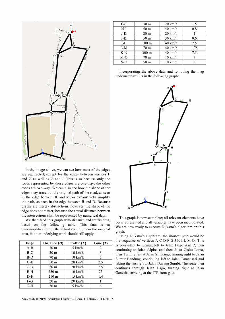
In the image above, we can see how most of the edges

are undirected, except for the edges between vertices F and G as well as G and J. This is so because only the roads represented by those edges are one-way; the other roads are two-way. We can also see how the shape of the edges may trace out the original path of the road, as seen in the edge between K and M, or exhaustively simplify the path, as seen in the edge between B and D. Because graphs are merely abstractions, however, the shape of the edge does not matter, because the actual distance between the intersections shall be represented by numerical data.

We then feed this graph with distance and traffic data, based on the following table. This data is an oversimplification of the actual conditions in the mapped area, but our underlying work should still apply.

Edge Distance (D) Traffic (F) Time (T) A-B 10 m 5 km/h 2 B-C 30 m 10 km/h 3 B-D 70 m 10 km/h 7 C-E 50 m 20 km/h 2.5 C-D 50 m 20 km/h 2.5 E-H 250 m 10 km/h 25 D-F 210 m 15 km/h 1.4 F-G 20 m 20 km/h 1 G-H 30 m 5 km/h 6

G-J 30 m 20 km/h 1.5 H-I 50 m 40 km/h 0.8 J-K 20 m 20 km/h 1 I-K 50 m 30 km/h 0.6 I-L 100 m 40 km/h 2.5

L-M 70 m 40 km/h 1.75 K-N 300 m 40 km/h 7.5 M-O 70 m 10 km/h 7 N-O 50 m 10 km/h 5

Incorporating the above data and removing the map

underneath results in the following graph:

This graph is now complete; all relevant elements have

been represented and all variables have been incorporated. We are now ready to execute Dijkstra’s algorithm on this graph.

Using Dijkstra’s algorithm, the shortest path would be the sequence of vertices A-C-D-F-G-J-K-I-L-M-O. This is equivalent to turning left to Jalan Dago Asri 2, then continuing to Jalan Alpina and then Jalan Cisitu Lama, then Turning left at Jalan Siliwangi, turning right to Jalan Sumur Bandung, continuing left to Jalan Tamansari and taking the first left to Jalan Dayang Sumbi. The route then continues through Jalan Dago, turning right at Jalan Ganesha, arriving at the ITB front gate.


IV. DISCUSSION

The case study above shows plausible results. Albeit oversimplified data, the study shows that it is indeed possible to determine the most efficient route by first representing a portion of a city map as a graph and then applying Dijkstra’s algorithm to find the shortest path.

In real-life application, pathfinding would involve a far greater number of vertices and edges spanning a wider area of the city. Say, for example, if the map used in our case study was not simplified, we would have at least twice the number of vertices. More data would be required regarding traffic, and more precise measurements of distance would help improve the quality of the process.

With regards to algorithm complexity, pathfinding using the method described above runs in the same amount of time as Dijkstra’s algorithm, added with the arithmetic of calculating T(E). If V is the number of vertices in the resulted graph and E is the number of edges, then our method would run in O(|V|2) + O(E). Since the algorithm complexity follows a quadratic pattern, applying this method in a real-life situation would require significantly more computation that our case study.

However, it should be noted that Dijkstra’s algorithm is the most efficient algorithm for finding the shortest path for graphs with non-negative weights, thus this method would be relatively the most efficient method of pathfinding using graph theory.

V. CONCLUSION

From the explanation above, it can be concluded that it is possible to route the most efficient route through traffic by means of using Dijkstra’s algorithm.

REFERENCES

[1] City map, http://en.wikipedia.org/w/index.php?title=City_map&oldid=461616441 (last visited Dec. 7, 2011).

[2] Graph (mathematics), http://en.wikipedia.org/w/index.php?title=Graph_(mathematics)&oldid=463999352 (last visited Dec. 7, 2011).

[3] Path (graph theory), http://en.wikipedia.org/w/index.php?title=Path_(graph_theory)&oldid=450267728 (last visited Dec. 11, 2011).

[4] Dijkstra's algorithm, http://en.wikipedia.org/w/index.php?title=Dijkstra%27s_algorithm&oldid=465227482 (last visited Dec. 11, 2011).

[5] http://www.cprogramming.com/tutorial/computersciencetheory/dijkstra.html

PERNYATAAN

Dengan ini saya menyatakan bahwa makalah yang saya tulis ini adalah tulisan saya sendiri, bukan saduran, atau terjemahan dari makalah orang lain, dan bukan plagiasi.

Bandung, 10 Desember 2011

Tubagus Andhika Nugraha 13510007

pathfinding through urban traffic using dijkstra’s...

Documents