path sequence-based xml query processing - inria
TRANSCRIPT

Path Sequence-based XML Query Processing
Ioana ManolescuINRIA Futurs–LRI
France
Andrei ArionINRIA Futurs–LRI
France
Angela BonifatiICAR CNR
Italy
Andrea PuglieseUniversity of Calabria
Italy
Abstract
We present the path sequence storage model, a new logical model for storing XML documents. This model partitions
XML data and content according to the document paths; and uses ordered sequences as logical and physical structures.
Besides being very compact, this model has a strong impact on the efficiency of XQuery evaluation. Its main advan-
tages are: fast and selective data access plans; intelligent combination of such plans, based on a summary of the document
paths; and intelligent usage of a concise path summary.
The model is implemented in the GeX1 system. We describe our physical storage scheme, query processing and
optimization techniques. We demonstrate the performance advantages or our approach through a series of experiments.
1 Introduction
XML data management has been a very active research field lately. The XQuery [25] W3C standard for XML querying has
almost reached its final state; accordingly, XML database research is concentrating on storage and processing techniques
for XQuery evaluation [2, 28, 21, 8, 12, 9, 15, 19, 7]. To illustrate the issues involved in XQuery processing, we use the
XMark [24] document snippet depicted in Figure 3(a). The document models an on-line auction site: clients, items for
sale, and a classification of items in categories. We use italic fonts for #PCData and attribute values.
Example 1. Consider the query:
for $i in //asia//item, $d in $i/description where $i//keyword=”romantic”
return � gift � � name � {$i/name} � /name � {$d//emph} � /gift �For every asian item and every description of this item, such that the item has at least one keyword descendent with
value “romantic”, the query returns a new gift element with the item name, and the emphasized points in its description.
Items with multiple “romantic” keywords must produce only one gift element, with the name and emph descendants if
any – or an empty gift element otherwise.
A central notion in XQuery evaluation is that of variable bindings. The bindings of a query variable � are the elements
(duplicate-free in the sense of element identity, and in document order) found by following the path expressions defining
� . For example, the bindings for $i consist of the unique, ordered elements found by matching the path expression
//asia//item. Similarly, bindings for $d are obtained by following //description from each binding of $i; $i bindings must
also be unique, and ordered.
1GeX stands for “The Gemo XML engine”.
1

Bind$k [="romantic"]
$d//emphBind
$dBind
Bind$i//name
Serialize
$i Bind
Combine
Figure 1: General XQuery evaluation strategy.
Algorithm loadPathSequences(document � )1 ����� = � ; ��� = � ; ���� �� ; ����� = �2 � = � ; � = ��� ; ����� � = � ; �"! = # # # # ; �"$ = # # # # ; %"! = � ; %"$ = �3 beginElement(tag � , attributes &('*)+� � )4 � = � ; �"$ =�"! ; %�$ = %"!5 � ++; � ! =� ! + # #-,.�/# # ; ����� .push([ � , -1])6 if the node of � ! is not yet created in ���7 then create it; let %"! be its number8 create �����10 % !�29 if ( �43 � ) then ��� .markBegin( % $ , % ! )
10 foreach &��+�657 98:&(��;<&�=(> in &('*)+� �11 create the container �"!?,�@7&�� in ��� if needed12 append ( � , &(= ) to this container13 characters(string A BC&�5D� )14 create the container � ! ,FEG�IHJ%C� in ��� if needed15 append 8:��;<AKBC&�5��.> to this container16 endElement( )17 ����� � ++; ����� .top.setPost(�C�D� � );18 append ����� .pop() to ������0 % !D219 ��� .markEnd( % ! )20 � = � ; � ! =� $ ; % ! = % $
Figure 2: XML document loading algorithm.
A generic query evaluation strategy in the spirit of [9]
follows from XQuery semantics [27]. Bind all the vari-
ables, and the subqueries in the return clause. Com-
bine these bindings through joins. Finally, serialize the
XML results, as dictated by the return clause. While
the previous phases manipulate mainly element IDs,
this step requires retrieving and tagging XML element
contents.
Figure 1 exemplifies this strategy for the query from
Example 1. We purposedly left unspecified the de-
tails of each step; we will discuss them later. No-
tice that the joins in Combine pair bindings accord-
ing to value-based predicates (none in this example),
or to structural relationships among the element IDs
they contain. The latter joins are known as structural
joins [2, 10, 8, 29]. In Figure 1, within Combine, a
structural join connects $i and $d bindings; a struc-
tural semijoin connects $i and $k, since items with sev-
eral matching keywords must produce only one result;
and structural outerjoins connect $name and emph el-
ements to $i and $d bindings, since a result must be
output even for items without name and/or emph descendents.
The performance of XQuery evaluation depends on the efficiency of these three steps: binding, combination, and
serialization. The latter can be done efficiently, once the content to be output has been gathered and ordered [20]. Thus,
performance is determined by: bindings variables, according to the query predicates, and the relationships between vari-
ables; and combining them.
Recent works provide efficient techniques for implementing [2] and ordering [28, 9] structural joins, relying on a
relational or tree-structured storage, augmented with B+-tree indexes [12, 9]. These indexes provide ordered access to the
identifiers of elements of a given tag. We call this storage and indexing approach tag partitioning (TP).
In this paper, we propose the new path sequence storage model. Our model partitions XML content and structure
according to the data paths, and stores it in ordered sequences. Its main advantage is its support for efficient variable
binding, up to several orders of magnitude faster than TP. This is due to the precise structural knowledge of the document,
included in the path sequence model. We make the following contributions:
L We describe the logical and physical path sequence storage model. This model is more compact than TP, and allows
for efficient document loading. The model comprises a document path summary, encapsulating compact structural
2

information.
L We show that based on the path summary, binding variables is much more efficient than when TP is used.
L We extend the iterator execution model, for operators whose output is in document order. Using path summary
information, and based on this extension, we derive a family of structural joins algorithms, which use selective
predicates on one input to access only the matching part of the other input.
L We show that our storage and query processing model integrates well with XQuery optimization techniques devel-
oped for TP [28, 9]. Besides more efficient evaluation options, our model also provides precise structural informa-
tions to the optimizer, further improving XQuery performance.
The paper is organized as follows. Section 2 describes the path sequence storage model. We then show how to ef-
ficiently answer XQuery queries based on this model. Section 3 discusses the construction of variable binding plans.
Section 4 addresses binding combination; the information from the path summary can be used to help an XQuery opti-
mizer. Section 5 presents the approach we take for XML serialization. Section 6 validates the interest of our techniques
through extensive experiments. We discuss related work in Section 7, and conclude in Section 8.
2 Path sequence-based storage
In this section, we describe the principles of path sequence-based XML storage, and its implementation options.
2.1 The logical path-sequence storage model
Our model separates the document structure from the document content, and stores each set of similar items in document
order. We decompose the document into three distinct structures, that we describe in turn.
The first structure contains a compact representation of the XML tree structure. We assign unique, persistent identifiers
to each element in an XML document. We adopt the [pre, post] scheme used in [2, 10, 12]. The pre number corresponds
to the positional number of the element’s begin tag, and the post number corresponds to the number of its end tag in the
document. Using this scheme, an element e � is an ancestor of an element e � iff n � .pre � n � .pre and n � .post � n � .post. For
example, Figure 3(a) depicts the [pre, post] ID of each element just above the element.
Furthermore, we partition the identifiers according to the data path to which the elements belong. Logically, each
partition is a sequence of identifiers, ordered by their pre field, which reflects the document order. For example, Fig-
ure 3(c) depicts a few path sequences resulting from the sample document in Figure 3(a), for the paths /site, /site/people,
/site/regions/asia/item etc.
All IDs in a path sequence appear at the same depth in the document tree, which is the path length. Thus, element
depth is concisely stored within the paths.
Our second structure stores the contents of XML elements, and values of the attributes. We pair such values to their
closest enclosing element identifier (precisely to the pre field of that element ID), and store them in a sequence of [pre,
3

[1 1000]/site/site/people [2 10]/site/people/person [10 9][3 7]
/site/regions/asia/item [19 66]
[10 9]
3[3 7] [1 1000]
1[2 10]2
@id="person0"
city
Tampa
[7 3]country
USA
[6 2]street
35 McCrossin St
[8 4]
lace umbrella
category
category
name
name
description
site
regions[17 300]
item ...
parlist
description
[1 1000]
[29 63]listitem
[22 64]
[21 65]
[19 66]
listitem[23 59]
[18 100]asia
name
item item
europe
item
[33 200]
... ...
people
person
[2 10]
emailaddress[9 6]
mailto:[email protected]
person
@id="person1"
name
T. Limaye
[13 11]
[14 51]
[15 12]
... ... ...
[16 50]
A special
text[30 60]
keyword[31 61]
romantic
emph
gift
[32 62]
From Paris
text[28 58]
address [5 5]
[3 7]
[10 9] [12 52]
[11 8]
[20 53]
parlist
listitem[25 56]
[24 57]
Ivory
emph[27 55]
text[26 54]
Umbrellaname
M. Wile
[4 1]
person1person0
[10 9]
3/@id[3 7]
27/#text[28 58]From Paris
people
person
site
regions
asia
item
description
parlist
listitem
listitem
parlist
europe
item
text keyword
1
2
3
4
16
15
1719
5
8
category
category
description
name
name
1112
13
14
10
name
67
address
countrycity
street
9emailaddress
text
emph
@id name18
2021
22 2324
25 26emph
27 28
2930
1 − site m =1 M =1N1=1 {2, 10, 15}
m =1 M =1
m =1 M =1
2,1
10,1
15,1
2 1 people N2=1{3}3,2
2,1
10,1
3,23,2
15,1
m =2 M =2
(c)
(d)
(a)
(e)
(f) 4/#text[3 7][10 9]
M. WileT. Limaye
/site/people/person/@id [3 7]person0
/people/person/name/#text [4 1]M. Wile
/site/regions/asia/item/description/parlist/listitem/text/#text
T. Limaye
person1
From Paris[28 58]
[11 8]
[10 9]
(b)
(g)
Figure 3: XMark document snippet, its path summary, and some of the resulting storage structures.
value] pairs ordered by pre. We call such a sequence a container.2 Values found in a container are classified as string,
integer, or double values; this can be inferred from their format. For example, Figure 3(e) shows some containers for the
document in Figure 3(a), for /site/people/person/@id, /site/people/person/name/#text etc.
To deal with XML elements having both textual and element children, we can assign IDs [pre, post] to each text child,
as if it were a text element. For example, the fragment � description � New � bold � Nike � /bold � sport shoes � /description �
would yield the IDs: [1, 4] for description, [3, 2] for bold, and [2, 1] and [4, 3] for the two text children of description. For
simplicity, in the rest of the paper, we ignore the mixed-content issue.
The above two structures alone can represent a document without any loss. We added a third indexing structure
that will prove very useful in query processing. The path summary of an XML document is a tree, whose internal
nodes correspond to XML elements, and whose leaves correspond to values (text or attributes). For every simple path��������������� �����
matching one or several (element or value) nodes in the XML document, there is exactly one node reached
by the same path in the path summary.
To each node � in the path summary, we assign an unique integer path number which characterizes both the node
and the path from the summary root to the node � . Thus, each path-driven ID sequence is uniquely associated to a path
number. Each container is associated to a pair of a path number, and: either @attrName for attributes, or #text for text
content. Figure 3(b) represents the path summary for the XML fragment at its left. Path numbers appear in large fonts
next to the summary nodes.
A path summary is different from a dataguide [11]. The former is always a tree, while the latter can be a graph.
Another relevant difference is that a dataguide tends to group nodes with the same tag, for example, a single dataguide
node would stand for the nodes 17 and 30 in Figure 3. We keep separate information about these element sets.
The path summary encapsulates a set of simple and concise statistics. Let � be a node in the summary, on a path
2The term is inspired from the XMill project [14].
4

ending with the tag � , and � be a child of � . We record in the path summary the following statistics:
L���� : the number of elements found on the path � (the size of the ID sequence corresponding to � ).
L���� � ����� � : the minimum, resp. maximum number of � children of the XML elements on the path � .
Notations. For a given document, we denote by � its size, � its height, and ����� the number of nodes in its path
summary. We show in Section 6.2.2 that the path summary is very small compared to the document, and thus we keep it
in memory at query processing time.
ID sequences, containers, and the path summary together are all the storage we materialize from a document, not
indexes to be added to another persistent storage. We now discuss the loading of a document within this model.
2.2 Document loading algorithm
We load an XML document in a single pass, using an event-based parser [26] which raises events while traversing the
document: beginElement on a start tag, characters when an element value is found, and endElement on an end tag.
Figure 2 shows the parser pseudo-code; it gradually construct the ID sequences ����� , containers � ��� , and path
summary ��� . At any point, the current element is the last one for which beginElement was raised; we identify it in
Figure 2 by � , and its parent by � . Their respective paths are �! and �#" , with path numbers �$ and �#" .
On beginElement, we save the current � in � (line 4) and assign a new � number. We push on %'&(� an incomplete) � �+*-,+. ID, since we don’t know its post value yet. If � is the first element encountered on its path, we create the
corresponding node in the path summary (lines 6-8). For each node � " and child � , ��� stores a temporary value
/10 � �324 �35 representing, for the most recently encountered element on path � " , the number of its children on path � . The
call to ��� markBegin (line 9) increases /60 � � 2 � 5 by , , and sets to 7 the counters /60 � � 5 �98 , for all children �;: of �$ . The
parser passes the attributes of � as parameters to beginElement, thus we append their values to the proper containers here
(lines 10-12).
On characters, we append the value to the correct container (lines 13-15).
On endElement, we compute the post number of � , update � ’s ID, and pop it from % &<� into the right sequence (lines
17-18). The ��� .markEnd call (line 19) updates � � 5 �38 and � � 5 �38 using the value /60 � � 5 �38 if needed.
The algorithm runs in time linear with � , using =?>@�BA � ���$C memory for the stack and path summary.
2.3 Physical storage for the path sequence model
An essential feature of the path sequence logical model is order in ID sequences, and in containers. Thus, the physical
storage structures implementing it must inherently support order. We consider two ordered persistent structures:
B+-trees. This is the option is considered in many works [8, 10, 12, 29], relying on a relational or persistent tree storage.
Its advantage is robustness, and good support for updates. Its disadvantage, as we show in Section 6.2.2, is the important
bloating factor due to extensive ID indexing.
5

Persistent sequences. The alternative that we investigate is the usage of persistent sequences as basic storage unit. The
advantage of this model is its extreme compactness, which leads to reduced memory usage. We found at least one persis-
tent storage system, endowed with locking and transaction functionality, supporting sequences as first-class citizens [6]. A
more recent system [13] features a sequence-based storage, largely outperforming an RDBMS in applications where data
order is critical (e.g., financial series data). The drawback of sequence-based storage is its poor behavior in the presence
of updates.
In this work, we focus on read-only querying. Thus, we adopt persistent sequences as physical storage.
Figure 3(d) represents the physical storage of the ID sequences in Figure 3(b). Items in these sequences have constant
length, equal to the ID size. Figure 3(f) depicts the sequences resulting from the containers in Figure 3(c). Container
entries have variable length, due to the data values. Thus, we use sequences of variable-length items.
We store the path summary as a sequence of variable-length items, as in Figure 3(g). There is one item per node,
comprising: the node number, its parent number, the children numbers, and the statistics previously described. The space
occupied by the path summary is linear in � ��� .
3 Binding plans on a path sequence storage
In this section, we show how to construct variable binding plans using the path sequence model. Binding plans output
identifiers of the elements to which the variables are bound.
Notations. A linear path expression (lpe) is an expression of the form: 8:=�� � > 8 ,�� ,�,F> ' �8 ,�� ,�,�> ' ������J8 ,�� ,F,�>6'� , where
each� �
is a tag or a � , the���
s are connected by�
or� �
, ����� 7 , and ��
is an optional query variable. We refer to � as
the length of lpe � � . We call an lpe of the form� � ��� � � �� ��� �
a simple lpe. In particular, each node of the path summary
corresponds to the simple lpe connecting it to the root. We say that two simple lpes are related, when the path summary
node of one of them is an ancestor of the other’s node. The path summary nodes matching an lpe � are those obtained by
top-down evaluation of the lpe against the path summary, considered as a data tree. We also say the simple lpes of these
nodes match � .
We consider a generic tuple-based execution model, following the iterator interface. We denote � � ) � . the�-th column
in the output of � � . Each column may be either of a simple type like string, integer etc., or of type structural ID.
3.1 Binding one query variable
The first problem we consider is binding a single variable to an lpe, such as $x in the query fragment “for $x in
/site/people/person/name”.
Path partitioning allows immediate access to the bindings: just scan the corresponding ID sequence, numbered 4 in
Figure 3. We use IDScan( � ) iterator, returning the IDs from the path sequence associated to � ; IDScan also fills in the
depth field in element identifiers, with the length of the simple lpe of � . Its output is ordered, and duplicate-free.
Now consider more complex lpes, as for example in the fragment “for $x in //parlist//text”. We identify the set of path
summary nodes matching //parlist//text. We scan all corresponding ID sequences, and at the same time merge them in a
6

pipelined fashion. The resulting bindings are in document order, and free of duplicates.
In general, we can retrieve the bindings for $x by matching � against the path summary into a set of elementary paths,
reading exactly the useful ID sequences, and merging them. No join is required.
Let � � be the number of nodes in the path summary matching � , � � be the number of bindings for � , and � be the
blocking factor.
Theorem 3.1 Using path partitioning, the bindings for � can be obtained with an % � = cost of =?> � � �� A � � C , and a
CPU cost of =?> � � � � ���B>�� � C C . The memory occupancy required is =?> � ��� A � � C .The % � = cost is due to scanning exactly the desired binding IDs. Each ID sequence is physically clustered, but all the � �matching sequences may not be clustered together, thus the � � extra reads.
The CPU cost corresponds to the merge of � � ordered ID sequences. The Merge operator uses a balanced search tree
with � � leaf nodes. Each ID read from one input is inserted in the search structure in =?> � ���;>�� � C C ; to produce an output,
the Merge extracts from the search structure the smallest ID it contains, again in =?> � ���;>�� � C C .The memory occupancy corresponds to holding the path summary, and the Merge’s search structure.
To match an lpe � against the path summary, we traverse the summary top-down, identifying the tags in � from left to
right, and adding nodes found to match the last tag in � to the result set. This can be done in =?> � ��� C time. For example,
to bind //asia//item, we start from node 1 with � , and attempt to match its first tag asia. Since the root has a different tag,
we propagate the search for � to all children of the root, which propagate it further. On the regions/asia branch, the asia
tag is matched, and the search for //item is propagated to its children etc.
Binding with simple predicates. Now consider simple selections on the text value, or attributes of $x, as in:
for $x in //people//person[@id=“person0”]
In such cases, we need to access the container for person/@id. We use a ContScan( � ) operator, where � is a container path
like 3/@id in Figure 3, returning the ordered [pre,value] container tuples. On top of ContScan, a selection can be applied.
If an index on the container exists, we use the IdxAccess operator to access only the desired tuples. We furthermore apply
a structural join with IDScan(4), to retrieve the complete [pre,post,depth] IDs.
Binding with more complex predicates. This case can be thought of as binding several variables, on some of which
there are simple predicates. For example, the following two fragments are equivalent:
for $x in //europe//item[//keyword=”romantic”]//price... and
for $x in //europe//item, $y in $x//price where $x//keyword=”romantic”...
We address many-variable binding next.
3.2 Binding several related variables
In general, bindings must be computed for several related variables. For example, Figure 4(a) depicts the query variables
from Example 1, structured in a generalized tree pattern (GTP) [9]. We use simple lines for�
relationships, and double
lines for� �
. Dashed lines denote left outerjoin connections between two nodes, considering the parent at left. Edges with
7

$k keyword="romantic"
$d description
asia
$2 emph $1 name
$i item*
$k keyword="romantic"
asia
$1 name
$i item
$2 emph
*
(a) (b)
IDScan(18)ContScan(18/#text)
STJ−FFD
STJ
TagContent
IndexAccess(28)IDScan(17)
STJ−FFA
STJ−FFD
IDScan(22)IDScan(18)ContScan(18/#text) ContScan(22/#text)
STJ STJ
Merge
Figure 4: Generalized tree pattern (a) and reduced pattern (b) for the query in Example 1 (left); complete query executionplan to be discussed throughout the paper (right).
a ’*’ denote left semijoin relationships (also considering the parent at left). We gave the ad-hoc names $1 and $2 to the
nodes corresponding to the return clause.
To bind such variables, we proceed in two steps. First, we determine the minimum data sets that need to be accessed to
bind the variables, by analyzing relationships among variables, and the path summary. In this step, we may also discover
useless variables, or new relationship among them. Second, we construct binding plans, based on the knowledge gathered
in the first step.
Variable path inference. We start by computing, for every variable, the set of paths in the path summary to which it
may possibly be bound. Throughout this section, let � , � be query variables such that � is a parent of � in the GTP, and
��� , ��� be their respective sets of possible paths.
We compute ��� sets by traversing the GTP and the path summary in parallel, using ��� as a starting point to determine
the ��� . For example, for the query in Figure 4 and the path summary in Figure 3, � � is {/site/regions/asia/item}. From
the node in � � , we match the /description path to find that ��� is {/site/regions/asia/item/description}. Similarly, matching
//keyword from � � yields the set � � ={28} (denoting paths by their numbers in Figure 3(b)). Using ��� and � � , we find
� � ={18} for $1 and � � ={22, 26} for $2.
Semijoin transformation. During path inference, for every edge connecting a parent variable � to a child variable � , and
pair of related paths �� � � , �� � � , we compute the maximum path factor � ��� � � . This factor is the maximum � �� �� found by traversing the path summary from node � to node � . For example, for the edge between $i and $2 in Figure 4(a),
we compute the � ��� ��� � � and � ��� ��� ��� ; � ��� ��� � � is the largest among � ��� ��� , � ��� ��� , � ��� � � , and � � � � � .
If � ��� � ��� , , and if the edge connecting � to � is a semijoin, we transform it into a join edge, since join and semijoin
coincide. For example, if � ��� ��� ��� � , in Figure 3, the execution of the query in Example 1 could start with an access
to $k, followed immediately by a join with the bindings for $i. Without this optimization, a duplicate-elimination step on
$i identifiers would be needed, when combining the bindings.
Join branch elimination. Similarly, we compute the minimum path factor � ��� � � for each related pair of paths � and � ,
as the minimum ��� � along the path from � to � . If the edge between � and � is a join, � ��� � � � , and � ��� � � � , for
all related paths � � � , and there is no predicate directly on � , then we eliminate � from the GTP, and “glue” all descendents
of � to � directly. For example, on the GTP in Figure 4(a), if all asian items have exactly one description, the variable $d
is useless and is eliminated, leading to the reduced GTP in Figure 4(b).
8

Algorithm traverse(GTPNodes � , % ,PSNodes ��� , ��% , �C= )
1 foreach GTP node = � child of �2 � HJ%C� � = % ; � HJ%C�6� � =�C%3 if (the tag of ��= matches the tag of = � )4 if ( = � is a variable node)5 mark( % , = � , �C% , ��= )6 upd( � ������� ��� , ������� ��� , ������ ��� , ����� ��� )7 � HJ%C� � = = � ; � H.%?�I� � =�C=8 foreach PSNode ��� child of ��=9 traverse( = � , � H.%?� � , ��= , � HJ%C�6� � , ��� )
10 if (the edge � - = � is ancestor-descendent)11 foreach PSNode ��� child of ��=12 traverse( � , % , ��= , ��% , ��� )
1516
$x
22
$y $t
26
17
$z
3029
$d $2
26
$1 $k$i
17 19 2218
28
Figure 5: The path inference algorithm, and sample results.
Variable path pruning. Next, we use each set � � to prune useless paths from � � , where � is a variable parent of � in the
GTP. For example, consider the query: for $p in //parlist, $k in $p//text return $k.
Path inference in this case yields ��� ={20, 23}, and � � ={26}. Since we know by the path summary that 26 is a descendent
of 20, but not of 23, we eliminate the useless path 23 from �� , which becomes {20}. Such pruning applies only when in the
GTP, � and � are connected by continuous edges only. It does not apply to children connected to their parents by dashed
edges, since these children are not required by the query. Thus, even ancestors that do not have them must produce results.
The same pruning may find that a query has no answer, due to an empty path set for a variable connected through
joins and semijoins only to the root.
GTP enrichment. Finally, new structural relationships among variables may be discovered. For example, consider the
fragment “for $i in //item, $p in $i//parlist, $t in $i//text”. After path inference and pruning, all paths of $t are descendents of
some path of $p. This translates into a new join edge from $p to $t, providing new possibilities of binding combination
(the GTP node set does not change).
The path inference algorithm. The algorithm is sketched in Figure 5. It consists of a recursive traversal function traverse
that is invoked on a path summary node � � , given: its parent summary node � � ; the last GTP node � that has been matched
to an ancestor of � � ; the last GTP variable node � that has been mached to an ancestor of � � 3; and the path � � where this
� was matched.
The invocation of traverse on � � aims to match � � to one of the (GTP) children of � . For each such child ��, we check
if the tag of � � matches that of ��. If, furthermore, �
�is a variable, then we mark the path we found for it, given that its
parent variable � was matched to the path � � (line 5). Furthermore, we update � ��� �+� � � and � ��� �+� � � with the � and
� statistics stored for � � and � � (line 6).
Next, whether ��
is a variable or not, we propagate the matching further by trying to match the children of ��
(in
the GTP) to the children of � � (in the path summary), through recursive calls (lines 8-9). For this call, the last variable
matched is � (that may have changed when matching ��), and the last GTP node matched is �
�.
Finally, if the edge beween � and ��
is ancestor-descendent, we also traverse � � ’s children with the same parameters
3Not all GTP nodes are variables; for example, the asia node in Figure 4 is not a variable, yet it has to be matched before its descendents.
9

as for � � . This ensures that // GTP edges are correctly matched at any depth in the path summary.
The worst-case complexity of this algorithm is =?> ������������ C , where ���$� is the size of GTP; this is consistent with
e.g. [18]. The worst case arises, for example, if the summary degenerates into a list of � ��� nodes labeled � , and the GTP
is a list of � ��$� //-connected nodes, labeled � . However, path summaries for real data sets are quite different, therefore,
this cost is affordable in practice. Furthermore, � � #� is rarely very large; and if all variables of the query do not have a
common ancestor, we have to solve several smaller, unrelated, matching problems.
The inference process outputs the path lists found for each variable, grouped hierarchically following the variables in
the GTP. In Figure 5, at the top right, we depicted the result for the query in Example 1. Each path found for a given
variable points to the corresponding paths found for its children variables in the GTP. (Arrows preserve all edge semantics
from the GTP; arrows leaving from the same path of a variable, and reaching different paths of another variable, have or
semantics.) Arrows are also annotated with the � ��� and � ��� computed factors.
Paths without required descendents are also pruned based on this result. For example, in Figure 5 at the bottom right,
we have depicted the paths resulting for the variables in: “$x in //regions, $y in $x/*, $z in $y/item, $t in $z//emph” on the
path summary in Figure 3. Realizing that path 30 for $z has no descendent path for $t, we prune 30, and then 29.
Semi-join transformation and join branch elimination also apply (and may reduce) on the result of path pruning.
Finally, to infer new edges in the GTP, we analyze the surviving variable paths. This process may be piggybacked on
traverse, using a matrix of ����� bits in which we mark which path is descendent of which other. The complexity of these
steps is still dominated by the path inference itself.
Binding plan construction. Using the path sets that result from the above steps, we construct individual binding
plans, as described in Section 3.1. For the query in Example 1, this yields: IDScan(17) for $i; Join(IDScan(28), Fil-
ter(ContScan(28/#text)) for $k; IDScan(19) for $1; Merge(IDScan(22), IDScan(26)) for $2 ($d has been eliminated).
These plans are selective, as they only access IDs whose paths allow them to contribute to the query result.
Metadata and statistics for the binding plans. Let� � � � denote the cardinality estimate for operator � � . If � � ) � . is of
type ID, we denote by ��� � � �1> � � � � C the set of path numbers on which IDs from � � ) � . may be found.
For IDScan( � ) plans, ��� � � �1> � � C ={ % },� � � � � � � . For plans of the form Merge(IDScan( � �
),��
, IDScan( � �)),
��� � � �1> � � C ={ % � , % � ,. . . % }, we estimate� � � � as � ��� ��� ��������� ��� � � . For Filter or IdxAccess plans, predicate selectivity esti-
mation are needed to estimate� � � � . Value statistics on containers can be used to this purpose.
4 Combining binding plans
Binding plans are combined bottom-up through joins and structural joins, as in [28, 9]. We now focus just on efficient
techniques enabled by the path sequence model, which can be profitably integrated to the combination step.
Section 4.1 derives from the path-based model an order-preserving condition for structural joins. Section 4.2 describes
more complex algorithms, that skip useless parts of the join inputs, enabled by our ordered path-partitioned storage.
Section 4.3 discusses the impact of our techniques on join ordering, and choice of physical operator.
10

d11 d12 d13
(b)
(a)
d1 d2 d3 d4 d5 d6 d7 d8 d9 d10
a1 a2 a3
a6 a7 a8 a9a4 a5
Figure 6: Structural joins when inputs can be skipped.
Algorithm STJ-FastForward( &�� A , ��H �JA )1 & = &(� A .getID(); � = ��H �JA .getID()2 while ( �.HJ� � 8:&�� AJ> or �JHJ�� 8:��HF�KAK> ) do3 if ( & is an ancestor/parent of � )4 then output [ & , � ]; � = ��H �JA .nextFF-pre(a.pre)5 else if ( � before & )6 then � = ��HF�KA � nextFF-pre( & .pre)7 else // & before �8 & = &(� A .nextFF-post( � .post)9 endwhile
Figure 7: The STJ-FastForward (STJ-FF) algorithm.
4.1 Order-preserving structural join
The StackTreeDesc (STD) and StackTreeAnc (STA) algorithms [2] directly apply in our context. They pair inputs by
structural relationships among structural [pre, depth, post] element IDs they contain. STA and STD require inputs sorted
in the document order of the IDs to join; STA preserves the order of the ancestor IDs, and STD the order of the descendent
IDs. Both algorithms employ a stack; STA needs some other data structures. Both work in pipeline.
To avoid intermediary sorting steps, it would be interesting to have a structural join operator preserving both ancestor
and descendent ID order; however, this is not always possible. For example, let � � � output successively the IDs [23,59],
[25,56], and let � � � return successively [26,54], [26,58]. The join result may be ordered in either order:
L ([23,59], [26,54]); ([23,59], [28,58]); ([25,56], [26,54])
L ([23,59], [26,54]); ([25,56], [26,54]); ([23,59], [28,58])
A structural join can preserve both input orders iff the IDs in the ancestor are free of ancestor-descendent pairs [2, 9].
This condition is data-dependent, and thus impractical to check. We provide a sufficient, easier to check condition:
Theorem 4.1 Let � � � and � � � be two operators, such that � � �) � . and � � �') � . contain element IDs. If the paths in
��� � � �1> � � � � � C are all pairwise unrelated, then a structural join matching ancestor IDs in � � � ) � . with descendent IDs
in � � � ) � . can preserve both input orders.
Given a set ��� � � � of size � , the condition can be checked on the path summary in =?> � � � C : from each node in ��� � � � , we
navigate upwards to the root; if we encounter another node from ��� � � � , then the paths are not pairwise unrelated. Thus,
when � � / paths are unrelated, the (simpler) STD algorithm can be used with the knowledge that it preserves both ancestor
and descendent order.
4.2 The STD-FastForward family of algorithms
A structural join may avoid reading parts of the inputs [29, 10, 8, 21]. Figure 6 depicts two such examples. Element IDs
are shown as horizontal [pre,post] segments, dashed for IDs of the � � / operator, and solid for IDs of the ��� �3/ operator.
An � � / ID � is an ancestor of a ��� �3/ ID � iff the segment of � is under the segment of � .
In Figure 6(a), the first descendent of � � is ��� . Thus, � � * ��� could be skipped, since they do not produce join results.
Instead, the join should advance ��� �3/ to the first � that may be a descendent of � � , that is, such that � pre � � � pre. Since
the ��� �3/ tuples are sorted on pre, it is possible to advance ��� �3/ according to this order.
11

In Figure 6(b), after the pair � � � � � � , the join could skip � � * � � , and advance �'� / to the first � that could be an ancestor
of � � � , that is, such that � post � � � �� post. This requires skipping on post, but the inputs are ordered on pre; the skip is
only possible if the two orders coincide. From the pre and post semantics, it is easy to see that these orders coincide in an
ID set iff it has no ancestor-descendent pairs.
A sufficient condition applies: Given an operator � � such that � � ) � . is of type ID, if ��� � � �1> � � � � C are pairwise unrelated,
then the pre and post orders in � � ) � . coincide.
Thus, we design the STJ-FastForward (STJ-FF) structural join algorithm; it is derived from StackTreeDesc, although
for readability we omitted the stack manipulation details. STJ-FF skips inputs both based on � � / .post and ��� �3/ .pre.
STJ-FF is depicted in Figure 7. It relies on two new methods provided by �'� / and ��� �3/ :L nextFF-pre( / � � , int � ) positions an operator � � to the first output tuple having � � ) / � � . .pre
� � . If such a tuple does
not exist, nextFF-pre returns false.
L nextFF-post( / � � , int � ) positions an operator � � to the first output tuple having � � ) / � � . .post� � . If such a tuple does
not exist, nextFF-pre returns false.
Using these methods, a parent operator commands its children to produce tuples with certain values only. They can only be
called on operators � � whose output is sorted on � � ) / � � . .pre; nextFF-post further requires that the paths in ��� � � �1> � � � / � � Cbe pairwise unrelated.
IDScan and ContainerScan operators implement the nextFF methods by binary search over the sequence. The Merge,
and the STJs, implement it combining calls to the nextFF methods of their child operators. An STJ supports: (�) nextFF-pre
on both the ancestor and descendent ID columns; (� �
) nextFF-post on the ancestor and descendent ID columns, if those
paths are unrelated. For example, let � � =STJ(IDScan(17), Merge(IDScan(21), IDScan(24))) in Figure 3. � � supports:
nextFF-pre on columns 7 and , , and nextFF-post on 7 only, since 21 and 24 are related.
In Figure 6(a), after the initial skip to � � , the region � � , � � , � � contains useful IDs. Thus, after finding � � , a binary
search to find � � would make useless effort. Therefore, we implement skipping “optimistically” in the IDScan and
ContScan operators: the next available value is examined, and only if it doesn’t satisfy the skip condition, binary search
is performed. This reduces skipping overhead when matching IDs are grouped, as we illustrate in Section 6.3.
Skipping in structural joins may lead to thrashing [29]. For skipping to be profitable, a certain threshold frequency of
useless IDs must be reached, starting from which skipping allows to scan less data. If a block is read for only one useful
ID, skipping the comparisons for the other ones will not bring noticeable benefits (Section 6.3).
The situations in Figure 6 do not always occur simultaneously. For example, consider “for $x in //person[id=”person0”],
$y in $x/name”. When joining bindings for $x and $y, there will be many useless $y bindings, and a single (useful) one
for $x. Thus, we specialize STJ-FF into: STJ-FFA, which only skips � � / tuples, and advances ��� �3/ through next() calls
only; and STJ-FFD, which only skips ��� �3/ tuples, and advances � � / through next(). We demonstrate their interest in
Section 6.3.
12

4.3 Optimizing with structural joins and path sequences
To evaluate a given structural join, the optimizer examines the operands’ ��� � � � � , and whenever ancestor ��� � � � � are
unrelated, it knows that both ordered will be respected. For example, all structural joins derived from the XMark [24]
queries feature unrelated �'� / paths.
The optimizer also needs to decide when to use skipping structural joins as those described in Section 4.2. For this,
cardinality estimates on binding plans, and structural join plans, are needed. In Section 3.2, we have shown how to
estimate the cardinality of individual binding plans. The estimation techniques described in [23] can be used to determine
the structural join plans size, based on the binding plan statistics. In [23], histograms are built on structural IDs of elements
satisfying a given set of elementary predicates, such as: having a given tag, or text value. Our framework provides more
precise elementary predicates, since we know from which path a given ID comes; similarly, value statistics are built on
path-partitioned containers. For example, for the query: “for $x in //person[@id=”person1”], $y in $x//age”, STJ-FFA is a
good join candidate, since $x is only bound to a single person.
To chose a join order, our optimizer relies on I/O cost and cardinality estimates for data access plans and join plans,
and on the interesting orders required and preserved by each operator, to avoid sorting steps whenever possible.
5 Serializing XML results
We now describe our strategy for constructing new XML results, and/or for retrieving full XML elements from the
database. Since the path partitioned model is very fragmented, those two tasks are exactly the same: any result element
must be (re)constructed piece by piece. For example, consider the query in Example 1, after the path inference and
simplifications described in Section 3.2. The query is internally brought to the form:
for $i in //asia//item where $i//keyword=”romantic”
return � gift � � name � $i/name/text() � /name � 5FHJA � � � � ($i//emph,{22,26}) � /gift �where 0 � / �9� � � is an internal reconstruction macro. This macro is unfolded into a GTP fragment as follows: the path
summary subtrees rooted at 22 and 26 are traversed entirely top-down, and outerjoin edges are added for all the data
elements contained. Finally, a Merge operator is added, since there are two different paths.
Figure 4(right) depicts the resulting complete QEPs for this query. It starts by joining $i bindings with bindings for
the “romantic” keywords; STJ-FFA skips useless item IDs. This is followed by two successive pipelined outerjoins for
$i/name and $i//emph. Both use STJ-FFD, since there are relatively few ancestors and many descendents. The TagContent
operator serializes XML contents out of a stream of tuples sorted and structured following the lines of [20].
In general, let � be a node in the path summary, % be the size of the path summary subtree rooted at � , and � be the number of attribute and content containers attached to these %9 nodes. Reconstructing elements on path � takes
%+ A � structural joins: one join to connect every node to its parent, and one to connect the containers. The leaves of
the reconstruction plan are IDScans and ContScans. For a very large number of outerjoins branches, materializing the
result of the for-where branches, such as the STJ-FFA in Figure 4(right), and performing the outerjoins separately may be
faster, since it prevents the outerjoins from building gradually very large intermediary results. The overhead is in keeping
13

intermediary results (ID tuples) in memory, which is in general affordable.
Despite the high degree of storage fragmentation, reconstruction is quite performant: (�) Each leaf operator reads data
on the correct path only; in the absence of selection predicates, the data read is exactly the data that must be returned. If
predicates apply, STJ-FF joins may skip useless descendents. (� �
) All joins preserve both orders (no sort).
6 Experimental validation
In this section, we present the implementation of the techniques previously presented within the GeX prototype (Sec-
tion 6.1). We assess the efficiency of our storage system for various XQuery processing tasks: storage conciseness and
binding plans (Section 6.2), binding plan combination (Section 6.3), and serialization (Section 6.4).
6.1 Hardware and software environment
We implemented the path sequence model in the GeX system. GeX is entirely implemented in Java; it consists of about
150 classes, or 40.000 lines of code. The GeX persistent storage is built on the BerkeleyDB [6] database library. We used
constant-size sequences for storing IDs, and variable-size ones for containers and the path summary. When container
indexes were needed, we built them using BerkeleyDB’s B+-trees.
Within the query engine, IDScan, ContScan, and IdxAccess operators interact directly with the BerkeleyDB storage.
The optimizer is similar to the one described in [9]; however, it constructs binding plans as described in Section 3 by
reasoning on the path summary, and uses the structural join operators described in Section 4.1, as explained in Section 4.3.
We ran GeX on a DELL D800 computer, with a Pentium III at 1.4 GHz and 1Gb of RAM, running RedHat Linux 9.0.
All times are averaged over 20 hot runs. We report results on: an XMark document of 118 Mb; the DBLP data set of 133
Mb; and the SwissProt dataset of 114 Mb, available at www.cs.washington.edu/research/xmldatasets.
6.2 Data storage and binding plans
6.2.1 Comparison baseline: tag partitioning
We compare our approach with the state-of-the-art XML storage model, based on partitioning, and structural identifiers.
Within this model, XML documents are stored as persistent trees or relational tables. Redundant B+-tree indexes are
added to the storage, indexing all element IDs by a (tag+pre) key. These indexes give access to the list of all IDs of
a certain tag. We call this approach tag partitioning (TP); it is used in [9, 12, 29]. We refer to our approach as path
sequences (PS).
In TP systems, index-based query processing is much faster than using the persistent tree or non-indexed tables. Thus,
we compare our query processing techniques with the techniques from [2, 28, 9] based on the tag indexes. To that purpose,
we implemented TP also, in two variants: using BerkeleyDB’s B+-trees, and by tag-based sequences. The latter can be
seen as merging all sequences (or containers) ending in the same tag, in a single sequence.
14

Figure 8: Space occupancy comparison for PS and TP. Figure 9: PS merging overhead when binding one variable.
6.2.2 Space occupancy
Figure 8 compares the space occupancy for PS, and TP using B+-trees as in [9, 12, 29]. For XMark, document structure
stored with PS takes about 10% of the document size; with TP, it takes 20 times more. This is due to the presence of tags
in the B+-tree keys (with PS, they are only stored in the path summary), and to the intermediary index pages. Overall, the
document size is multiplied by 3.5-4 by when stored with TP, close to the factor of 4 reported in [9]; with PS, the storage
size is slightly smaller than the document.
The path summary occupies 26 Kb for XMark, 6 Kb for DBLP, 10 Kb for SwissProt; ��� � is respectively 514, 122,
and 117. This validates the assumption that it can be kept in memory when processing queries.
Having demonstrated sequence conciseness, in the following, we report on PS and TP performance on a persistent
sequence-based storage. We have experimented query processing on TP-based B+-trees also, using a specific set of
IDScan and ContScan operators; the overall observations are the same.
6.2.3 Variable binding performance
In this section, we compare TP and PS binding performance. Without loss of generality, we mainly consider lpes where
tags are connected by //; the / case is similar.
The case most favorable to TP is a variable bound to a lpe of the form //tag: PS merges several IDScans (Section 3.1),
while TP only looks up the IDs of the given tag. When only one path summary node matches //tag, PS and TP coincide.
Figure 9 compares the execution time for binding plans when the TP and PS plans differ. The lpes used are: � �=//item,
� �=//description, ��� =//bold, � � =//category on XMark; � � =//title, � � =//author on DBLP; and � � =//Descr on SwissProt.
The cardinalities of the binding plans range from 2.000 ( � �) to 720.000 ( � � ). The PS overhead, due to scanning and
merging different sequences, is negligible. This is because: (�) the Merge is pipelined, CPU-only, and efficient due to the
ordered tree of inputs it maintains; (� �
) IDs are tightly packed by PS in sequences and read sequentially, thus no thrashing
occurs; (� �
) the Merge fan-out is of the order of hundreds, making it possible to keep in memory one block from each
sequence to be merged.
Binding a variable to longer lpes. In such cases, TP is handicapped by its unselective data access. For example, let �be /site/people/person/name: TP only allows to access all name IDs. Most of such IDs are not on the required path; they
may be on paths 11, 18 etc. (Figure 3), leading to useless data scans. To separate just the person names, we must access
15

Figure 10: Binding one variable to lpes of length 2. Figure 11: Binding one variable to lpes of length 3.
all person IDs (thus read even more data !), and apply a structural join between the two. Furthermore, we must read all
site and people IDs, and successively join with them also, to separate just the proper names.
In general, to bind a variable to a lpe of length � , TP must scan the IDs of all tags involved, and compute an � -way
join. PS just scans the result. (although we only need the IDs of the elements of tag� �
). Contrast this with theorem ??.
Now consider the query “for $x in //parlist//text”. TP must join all parlist IDs with all text IDs; but a new complication
arises. A text ID may be a descendent of two parlist elements, as is the case for the element [26,54] in Figure 3. Such text
elements will appear twice in the join result. Thus, a final duplicate elimination (dup-elim) is required.
Optimized TP. To give TP a chance, we use the PS path summary to eliminate useless data scans, joins, and dup-elims
from TP binding plans.
Let � be a linear path expression of length � , � � � ��� � �� � ��� ����� ��� � � ��� �
���� � �� � �����
, �3� be the set of path summary
nodes matching � , and ���� be the set of nodes matching � � � ����� � �� � ��� ����� ��� �
�� � � �� � �����
(� �
has been skipped). If
���� � �3� , then � � is equivalent to � ; reading and joining the IDs with the tag� �
can be avoided, reducing the binding cost.
In general, more than one such tag���
can be eliminated; for example, from //site//people//person//name we can eliminate
site, and person. There may be several minimal-length lpes equivalent to � ; both //people//name and //person//name are
equivalent to the previous path, and cannot be further reduced. Once � � and ���� are known, we can decide if ���� � � � in
=?> ����� � � C (look for a node labeled� �
between� ���
and� ���, in all ���� paths). To find the minimal equivalent path(s),
we test ��� �� against �3� for all subsequences � � � of � . We call optimized TP (OTP) the most efficient binding plan derived
from all the resulting minimal sequences. This binding plan only applies the final dup-elim if it is necessary: that is, if
two paths in � � are related. We now compare the binding performance of: PS, TP, and OTP. TP and OTP use the best
structural join ordering.
Figure 10 considers lpes of length 2: � � =//description//parlist, � � =//parlist//listitem, � ���=//item//keyword,
� � �=//person//name, � � �
= //category//name on XMark; � �� =//article//title, � � � =//book//author and � � � =//book//title on
DBLP; � ���=//METAL/Descr and � ���
=//LIPID//Descr on SwissProt. For � � and � � , PS and OTP coincide; TP performs
one extra join and a dup-elim. From � � �to � ���
, OTP only spares the dup-elim, which is cheap since the join result order
was favorable. The performance difference between PS and OTP reflects the proportion of useless IDs scanned by OTP
due to the tag-partitioned storage. This proportion reaches 430 for � � � ; PS is very fast for � � � , � � � and � ���.
In Figure 11 we measured lpes of length 3 (not listed for space reasons). (O)TP performance is determined by the data
16

� $x in //person, $y in $x//name, $z in $x//watch �� $x in //item, $y in $x//parlist, $z in $x//keyword � $x in //asia, $y in $x//item, $z in $x//description �� $x in //categories, $y in $x//listitem, $z in $x//text�� $x in //item, $y in $x//description, $z in $x//parlist �� $x in //article, $y in $x//title, $z in $x//year
Figure 12: Binding 2- and 3-variable patterns.
scans; PS speed-up is of up to several hundreds.
Overall, the TP handicap grows with the length of the lpe, as this translates to potentially more useless ID scan.
Path summary processing. We have measured the time to apply the path inference, simplification, and GTP enrichment,
as described in Section 3.2, on GTPs of up to 10 variables, derived from XMark queries. We found this time to be
negligible; the longest value was 0.145 s.
6.3 Combining variable bindings
In this section, we study binding performance for GTPs of two or more variables. Figure 12 compares TP and PS
performance when binding two, respectively, three related variables. Differently from the previous section, in these cases,
TP cannot benefit from any optimization, since the scans and the structural join are required, in order to get binding pairs.
Furthermore, PS must also scan many inputs and join them. Also, in Figure 12, PS and TS use the best possible join order.
In Figure 12 (left), we consider again the paths � � to � ���that we used in Figure 10, but this time we replace “for $x in
//tag � //tag � ” with “for $x in //tag � , $y in $x//tag � ”. For example, in Figure 12(top), � �� stands for the two-variable pattern “for
$x in //description, $y in $x//parlist”. We notice that for � �� and � �� , PS and TP are very close, since: TP makes no useless
reads (all parlist elements are under description elements, and similarly for � �� ), and the cost is dominated by data access.
For � ���� - � ���� , the unselective scans of TP translate directly into huge performance differences with PS; the curves mirror
quite closely those from Figure 10 (top). The biggest time we measured for the join in itself was 4.2 seconds, for � ���� .In Figure 12 (right), we consider a set of three-variable patterns, � �
- � � on XMark and � � on DBLP, shown just
underneath the corresponding graph.
While quite small, these patterns illustrate well the performance issues involved. We have chosen just 1-tag lpes to
connect $x to $y and $z, to pick the best possible case for TP: if longer paths connect variables, TP will do useless scans
and joins, as explained in the previous section.
Overall, scan, join, and total time are still smaller for PS than for TP. For � �, � � , � � and � � , the join cost is negligible
for both, compared to the data scan cost. In these cases, simply using a PS storage provides for faster binding. For � �and
� � , the joins by themselves take a more important part; even with the best ordering, the first join creates many intermediary
results, on which the second join spends more time. This problem can be alleviated using holistic twig joins [8], which
17
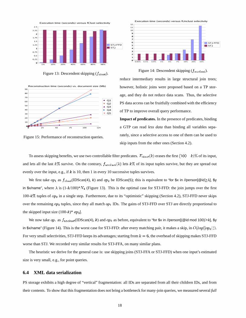
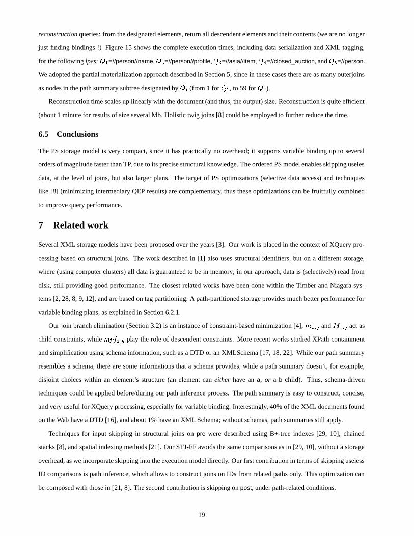
Figure 13: Descendent skipping ( ����� � ��� ). Figure 14: Descendent skipping ( � � ��� � � � ).
Figure 15: Performance of reconstruction queries.
reduce intermediary results in large structural join trees;
however, holistic joins were proposed based on a TP stor-
age, and they do not reduce data scans. Thus, the selective
PS data access can be fruitfully combined with the efficiency
of TP to improve overall query performance.
Impact of predicates. In the presence of predicates, binding
a GTP can read less data than binding all variables sepa-
rately, since a selective access to one of them can be used to
skip inputs from the other ones (Section 4.2).
To assess skipping benefits, we use two controllable filter predicates.� ��� � � � > � C erases the first > , 7'7 * � C�� of its input,
and lets all the last � � survive. On the contrary, � � ��� � ��� > � C lets � � of its input tuples survive, but they are spread out
evenly over the input, e.g., if � is 10, then 1 in every 10 successive tuples survives.
We first take � � � as � ��� � ��� (IDScan(4), � ) and � � � be IDScan(5); this is equivalent to “for $x in //person[@id �� ], $y
in $x/name”, where is (1- � /100)* � � (Figure 13). This is the optimal case for STJ-FFD: the join jumps over the first
100- � � tuples of � � � in a single step. Furthermore, due to its “optimistic” skipping (Section 4.2), STJ-FFD never skips
over the remaining � � � tuples, since they all match � � � IDs. The gains of STJ-FFD over STJ are directly proportional to
the skipped input size (100- � )*� � � � � .
We now take � � � as � � ��� � � � (IDScan(4), � ) and � � � as before, equivalent to “for $x in //person[(@id mod 100) ��� ], $y
in $x/name” (Figure 14). This is the worst case for STJ-FFD: after every matching pair, it makes a skip, in =?> � ���;> � � � ��� C C .For very small selectivities, STJ-FFD keeps its advantages; starting from � �� , the overhead of skipping makes STJ-FFD
worse than STJ. We recorded very similar results for STJ-FFA, on many similar plans.
The heuristic we derive for the general case is: use skipping joins (STJ-FFA or STJ-FFD) when one input’s estimated
size is very small, e.g., for point queries.
6.4 XML data serialization
PS storage exhibits a high degree of “vertical” fragmentation: all IDs are separated from all their children IDs, and from
their contents. To show that this fragmentation does not bring a bottleneck for many-join queries, we measured several full
18
reconstruction queries: from the designated elements, return all descendent elements and their contents (we are no longer
just finding bindings !) Figure 15 shows the complete execution times, including data serialization and XML tagging,
for the following lpes: � �=//person//name, � �
=//person//profile, � � =//asia//item, � � =//closed_auction, and � � =//person.
We adopted the partial materialization approach described in Section 5, since in these cases there are as many outerjoins
as nodes in the path summary subtree designated by � � (from 1 for � �, to 59 for � � ).
Reconstruction time scales up linearly with the document (and thus, the output) size. Reconstruction is quite efficient
(about 1 minute for results of size several Mb. Holistic twig joins [8] could be employed to further reduce the time.
6.5 Conclusions
The PS storage model is very compact, since it has practically no overhead; it supports variable binding up to several
orders of magnitude faster than TP, due to its precise structural knowledge. The ordered PS model enables skipping useles
data, at the level of joins, but also larger plans. The target of PS optimizations (selective data access) and techniques
like [8] (minimizing intermediary QEP results) are complementary, thus these optimizations can be fruitfully combined
to improve query performance.
7 Related work
Several XML storage models have been proposed over the years [3]. Our work is placed in the context of XQuery pro-
cessing based on structural joins. The work described in [1] also uses structural identifiers, but on a different storage,
where (using computer clusters) all data is guaranteed to be in memory; in our approach, data is (selectively) read from
disk, still providing good performance. The closest related works have been done within the Timber and Niagara sys-
tems [2, 28, 8, 9, 12], and are based on tag partitioning. A path-partitioned storage provides much better performance for
variable binding plans, as explained in Section 6.2.1.
Our join branch elimination (Section 3.2) is an instance of constraint-based minimization [4]; � � � and ��� � act as
child constraints, while � ��� � � play the role of descendent constraints. More recent works studied XPath containment
and simplification using schema information, such as a DTD or an XMLSchema [17, 18, 22]. While our path summary
resembles a schema, there are some informations that a schema provides, while a path summary doesn’t, for example,
disjoint choices within an element’s structure (an element can either have an a, or a b child). Thus, schema-driven
techniques could be applied before/during our path inference process. The path summary is easy to construct, concise,
and very useful for XQuery processing, especially for variable binding. Interestingly, 40% of the XML documents found
on the Web have a DTD [16], and about 1% have an XML Schema; without schemas, path summaries still apply.
Techniques for input skipping in structural joins on pre were described using B+-tree indexes [29, 10], chained
stacks [8], and spatial indexing methods [21]. Our STJ-FF avoids the same comparisons as in [29, 10], without a storage
overhead, as we incorporate skipping into the execution model directly. Our first contribution in terms of skipping useless
ID comparisons is path inference, which allows to construct joins on IDs from related paths only. This optimization can
be composed with those in [21, 8]. The second contribution is skipping on post, under path-related conditions.
19

GeX started as an XML querying and compression engine [5]; the work reported here is independent of compression.
8 Conclusion and future work
We have presented the path sequence storage model, a compact and fragmented model for XML storage. The path
sequence model improves over similar systems by preserving precise path information, in the storage as well as under the
form of a path summary that is extensively used for query optimization. Our model is fully implemented within the GeX
system; we validated its performance advantages through a series of experiments.
In the future, we envision extending GeX with support for updates, and schemas. For what concerns updates, using
the path inference algorithm described in Section 3.2 on an XML declarative update statement, it is possible to infer if
the update will create new paths, or move nodes from some paths to others. Thus, although the path summary is derived
from the data, it is possible to maintain it through document updates. With respect to schemas, we plan to find a simple
compromise between schema language conciseness, and difficulty of query minimization, based on the results of [18, 17].
Acknowledgements. The authors are extremely grateful to Alberto Lerner, for many useful comments on this paper.
References[1] Vincent Aguilera, Frederic Boiscuvier, Sophie Cluet, and Bruno Koechlin. Pattern tree matching for XML queries. Gemo Technical Report
number 211, 2002.[2] S. Al-Khalifa, H.V. Jagadish, J.M. Patel, Y. Wu, N. Koudas, and D. Srivastava. Structural joins: A primitive for efficient XML query pattern
matching. In ICDE, 2002.[3] S. Amer-Yahia. Storing techniques and mapping schemas for XML. Submitted for publication, 2003.[4] S. Amer-Yahia, S. Cho, and L. Lakshmanan et al. Minimization of tree pattern queries. In SIGMOD, 2001.[5] A. Arion, A. Bonifati, G. Costa, S. D’Aguanno, I. Manolescu, and A. Pugliese. Efficient query evaluation over compressed XML data. In EDBT,
2004.[6] The BerkeleyDB database library. http://www.sleepycat.com.[7] Omar Boucelma, Mehdi Essid, Zoe Lacroix, Julien Vinel, Jean-Yves Garinet, and Abdelkader Betari. VirGIS: Mediation for geographical infor-
mation systems. In ICDE, 2004.[8] N. Bruno, N. Koudas, and D. Srivastava. Holistic twig joins: Optimal XML pattern matching. In SIGMOD, 2002.[9] Z. Chen, H.V. Jagadish, L. Lakshmanan, and S. Paparizos. From tree patterns to generalized tree patterns: On efficient evaluation of XQuery. In
VLDB, 2003.[10] S. Chien, Z. Vagena, D. Zhang, and V. Tsotras. Efficient structural joins on indexed XML documents. In VLDB, 2002.[11] R. Goldman and J. Widom. Dataguides: Enabling query formulation and optimization in semistructured databases. In VLDB, Athens, Greece,
1997.[12] A. Halverson, J. Burger, L. Galanis, A. Kini, R. Krishnamurthy, A.N. Rao, F. Tian, S. Viglas, Y. Wang, J.F. Naughton, and D.J. DeWitt. Mixed
mode XML query processing. In VLDB, 2003.[13] A. Lerner and D. Shasha. Aquery: Query language for ordered data, optimization techniques, and experiments. In VLDB, 2003.[14] H. Liefke and D. Suciu. XMILL: An efficient compressor for XML data. In SIGMOD, 2000.[15] A. Marian and J. Simeon. Projecting XML documents. In VLDB, 2003.[16] L. Mignet, D. Barbosa, and P. Veltri. The XML web: A first study. In Proc. of the Int. WWW Conf., 2003.[17] J. Miklau and D. Suciu. Containment and equivalence for an XPath fragment. In Proc. of the Symposium on Principles of Database Systems
(PODS), 2003.[18] F. Neven and T. Schwentick. XPath containment in the presence of disjunctions, DTDs, and variables. In Proc. of the Int. Conf. on Database
Theory (ICDT), 2003.[19] Tuyet Tram Dang Ngoc and Georges Gardarin. Evaluating XQuery in a full-XML mediation architecture. In Proc. Journées Bases de Données
Avancées, 2003.[20] J. Shanmugasundaram, E. Shekita, R. Barr, M. Carey, B. Lindsay, H. Pirahesh, and B. Reinwald. Efficiently publishing relational data as XML
documents. In VLDB, Cairo, Egypt, 2000.[21] J. Teubner, T. Grust, and M. van Keulen. Bridging the GAP between relational and native XML storage with staircase join. In VLDB, 2003.[22] P. Wood. Containment for XPath fragments under DTD constraints. In Proc. of the Int. Conf. on Database Theory (ICDT), 2003.[23] Y. Wu, J.M. Patel, and H.V. Jagadish. Estimating answer sizes for XML queries. In Proc. of the Conf. on Extending Database Technology (EDBT),
2002.[24] The XMark benchmark. www.xml-benchmark.org, 2002.[25] The XQuery language. www.w3.org/TR/xquery, 2003.[26] The SAX project. www.saxproject.org.[27] XQuery 1.0 formal semantics. www.w3.org/TR/2004/WD-xquery-semantics.[28] H. Jagadish Y. Wu, J. Patel. Structural join order selection for XML query optimization. In ICDE, 2003.[29] C. Zhang, J. Naughton, D. DeWitt, Q. Luo, and G. Lohman. On supporting containment queries in RDBMSs. In SIGMOD, 2001.
20