path-loss channel models for receiver spatial diversity...

Research ArticlePath-Loss Channel Models for Receiver Spatial DiversitySystems at 2.4GHz

Abdulmalik Alwarafy,1 Ahmed Iyanda Sulyman,1 Abdulhameed Alsanie,1

Saleh A. Alshebeili,1,2 and HatimM. Behairy3

1Department of Electrical Engineering, King Saud University, Riyadh, Saudi Arabia2KACST-TIC in RF and Photonics for the e-Society (RFTONICS), Department of Electrical Engineering, King Saud University,Riyadh, Saudi Arabia3National Center for Electronics and Photonics Technology, King Abdulaziz City for Science and Technology, Riyadh, Saudi Arabia

Correspondence should be addressed to Abdulmalik Alwarafy; [email protected]

Received 27 January 2017; Revised 21 March 2017; Accepted 23 March 2017; Published 13 April 2017

Academic Editor: Ikmo Park

Copyright © 2017 Abdulmalik Alwarafy et al. This is an open access article distributed under the Creative Commons AttributionLicense, which permits unrestricted use, distribution, and reproduction in any medium, provided the original work is properlycited.

This article proposes receiver spatial diversity propagation path-loss channel models based on real-field measurement campaignsthat were conducted in a line-of-site (LOS) and non-LOS (NLOS) indoor laboratory environment at 2.4GHz. We apply equalgain power combining (EGC), coherent and noncoherent techniques, on the received signal powers. Our empirical data is used topropose spatial diversity propagation path-loss channel models using the log-distance and the floating intercept path-loss models.The proposed models indicate logarithmic-like reduction in the path-loss values as the number of diversity antennas increases.In the proposed spatial diversity empirical path-loss models, the number of diversity antenna elements is directly accounted for,and it is shown that they can accurately estimate the path-loss for any generalized number of receiving antenna elements for agiven measurement setup. In particular, the floating intercept-based diversity path-loss model is vital to the 3GPP and WINNERII standards since they are widely utilized in multi-antenna-based communication systems.

1. Introduction

Diversity is a robust communication technique utilized inmodern wireless systems to improve the quality of thereceived signals and to ensure a better link performance. Itis basically used to mitigate the effects of fading experiencedby a receiver in flat fading channels. The general concept ofdiversity is implemented through using diverse communica-tion channels each with different operating characteristics.This will guarantee better signal quality and thus better biterror rate (BER) performance, better signal-to-noise-ratio(SNR), and better signal coverage. The most commonly usedimplementation approaches for diversity systems in wirelesstransmissions are frequency diversity, spatial diversity, timediversity, coding diversity, and polarization diversity. Each ofthese approaches achieves a significant improvement in thewireless link performance [1]. The most efficient and widelyused implementation in modern wireless communication

systems however is the spatial diversity [1]. For example,the multiple-input multiple-output (MIMO) communicationsystems employed multiple spatial antenna elements at boththe transmitter (TX) and the receiver (RX) sides to boostsignal level and hence to increase the SNR. These MIMO-based systems are now implemented in a wide variety ofwireless systems such as the wireless local area networksWLANs (i.e., IEEE 802.11n/ac), theWiMAX, and the Fourth-Generation Long Term Evolution (4G-LTE) for cellularsystems. The most commonly utilized combining techniquesin spatial diversity are selection combining (SC), equal gaincombining (EGC), and maximal ratio combining (MRC)schemes [1–4]. The SC only requires an individual receiverand a basic phasing circuitry for each diversity branch. Inthe EGC, the weights of each branch are set to unity and thesignals of each branch are combined either without cophasing(noncoherently) or with cophasing (coherently). In MRC,however the signals from all the diversity branches are

HindawiInternational Journal of Antennas and PropagationVolume 2017, Article ID 6790504, 12 pageshttps://doi.org/10.1155/2017/6790504

https://doi.org/10.1155/2017/6790504

2 International Journal of Antennas and Propagation

weighted according to their individual SNRs, cophased, andthen summed. The SNR enhancements over a flat Rayleighfading channel as a function of the number of diversityantennas combined for these three techniques reveal thatEGC has slightly less SNR gain enhancement compared toMRC [1]. However, our measurement work here uses theEGC scheme since it is moderate in complexity, as it onlyneeds information about the phases of the signals. TheMRC,on the other hand, is more complex to implement since anestimation of both phases and amplitudes of the signals mustbe realized [2, 5], which is difficult to be achieved with ourequipment.

There are many works that have introduced path-lossmodels for single-input single-output (SISO) schemes, suchas the works in [6, 7]. However, despite the implementationof spatial diversity techniques in modern wireless commu-nications, no work to-date has incorporated spatial diversityantennas in path-loss models. For example, the works in [8–12] presented path-loss models for MIMO systems; howeverthesemodels do not have any term that accounts for the effectof the number of receiving diversity antennas. The authorin [13] conducted spatial diversity measurement campaignsin a modern factory at 2.4GHz to obtain path-loss models.However, there is no term in the presented path-loss modelsthat accounts for the number of antenna elements. Thework in [14] proposed a theoretical-based diversity gainmodel, which accounts for the number of antenna elements.However, since there is no distance-dependent term in themodel, it is not like the traditional path-loss models in theliterature.

Our previous works in [15, 16] proposed a receiverspatial diversity and a beam combining path-loss model,respectively, based on the log-distancemodel. However, sincethe floating intercept model (FIM) is also widely used in theliterature, for example, in the 3GPP [17] andWINNER II [18]standards, which are widely utilized in multi-antenna-basedsystems, it becomes imperative to develop such a receiver spa-cial diversity model in accordance with these standards. Thiswork proposes a receiver spatial diversity propagation path-loss channel model based on the FIM at 2.4GHz. We presenta comprehensive analysis of our path-loss measurement datathat were collected in an indoor environment at 2.4GHz.Theproposed receiver spatial diversity models present terms thataccount for the effects of the number of receiving antennaelements in the path-loss equations.

The rest of this article is organized as follows. Section 2discusses the equal gain power combining (EGC) procedurewith the related combining types. Section 3 illustrates theexperimental procedure and the LOS and NLOS propagationscenarios. Section 4 introduces the measurements-basedpath-loss channel models and analyzes them. Section 5presents the proposed spatial diversity path-loss channelmodels and, finally, Section 6 summarizes the article.

2. Equal Gain Power Combining Procedure

In order to improve the performance of wireless link, weemploy equal gain power combining (EGC) at the RX side.

Two combining schemes are adopted in our work, the non-coherent combining (NCC) and the coherent combining(CC) each of which will combine the power of the receivedsignals that arrive from the receiving diversity antennas.The potential enhancement that is achieved from these twoschemes are quantitatively investigated by means of theaverage enhancement (i.e., reduction) in the path-loss andby means of the percentage of the path-loss exponent (PLE)reduction relative to the single antenna reception case (i.e.,SISO system) as well as by means of cumulative distributionfunction (CDF). In CC scheme, the received powers fromeach RX diversity antenna are cophased and aligned, sothey can be combined together using a known carrier phaseinformation [1, 2, 5]. This enables us to extract the maximumpower from each diversity antenna element.TheNCC, on theother hand, assumes that signals phases from each individualreceiving diversity antenna are independently and identicallydistributed (i.i.d). This means that we can directly linearlyadd the powers from each antenna without the need for anyalignment or phase information [1, 2, 5].The CC and NCC ofthe received spatial diversity powers, that is, 𝑃𝑟CC and 𝑃𝑟NCC,are given, respectively, by [2]

𝑃𝑟CC (𝑑) = (𝑁𝑟∑𝑖=1

√𝑃𝑖)2

, (1)

𝑃𝑟NCC (𝑑) =𝑁𝑟∑𝑖=1

𝑃𝑖, (2)

where 𝑃𝑖 is the received power inWatts and𝑁𝑟 is the numberof receiving antenna elements. We used these two combiningschemes on our measurement data, for power received fromtwo, three, or more receiving diversity antennas. The cor-responding log-distance and floating intercept propagationpath-loss channelmodels are then developed for cases of line-of-site (LOS) and non-LOS (NLOS) propagation scenarios.

3. Experimental Procedure

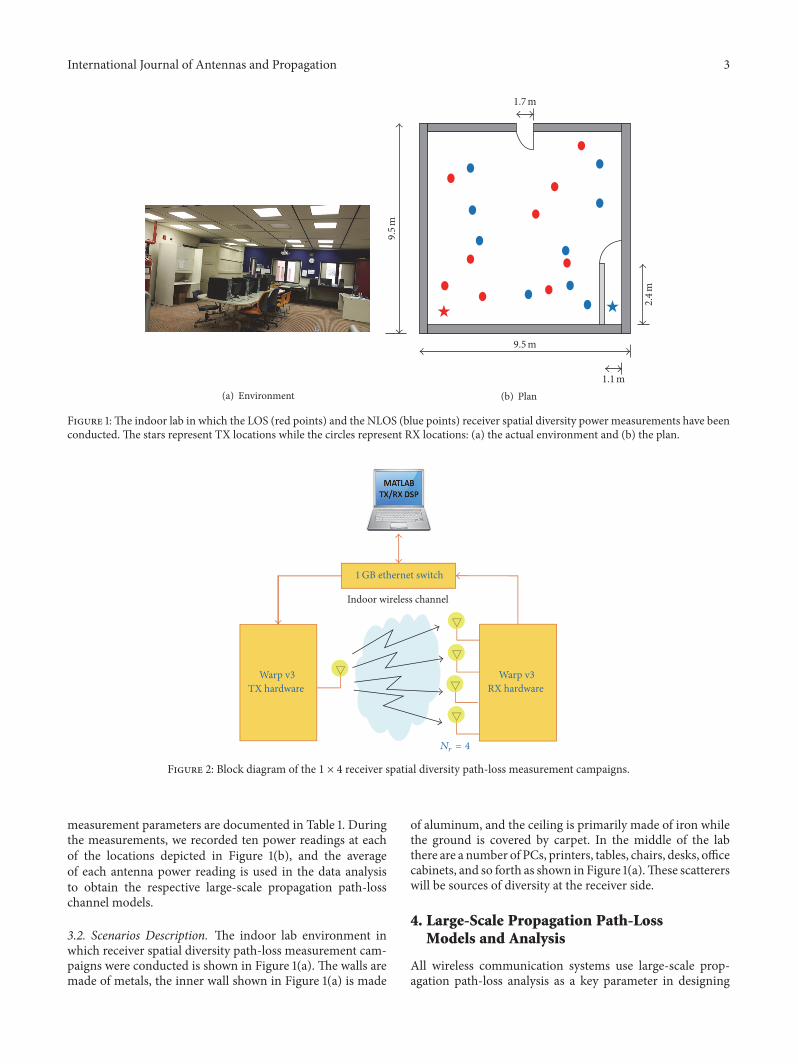
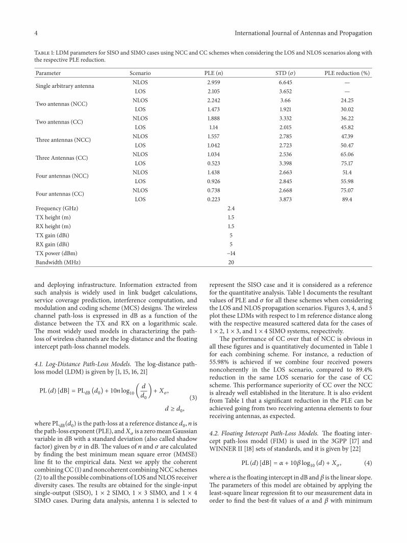
3.1. Measurements Setup. The test signal that is used in ourreceiver spatial diversity indoor measurement campaigns isgenerated using the Warp v3 kit [19], similar to the experi-ments conducted in [15, 20]. In our experiments, we selectedone LOS and one NLOS transmitter location and randomlyselected nine LOS and nine NLOS locations scattered inan indoor, stationary, laboratory environment with TX-RXseparation distances up to 9m. Figure 1 shows the indoorlab environment along with the corresponding LOS andNLOS measurement locations. At each TX-RX LOS/NLOSlocation, one TX antenna and up to four RX antennas wereused (i.e., 1 × 4 single-input multiple-output 1 × 4 SIMOsystem). Figure 2 shows the block diagram of the 1 × 4receiver spatial diversity that is used in the measurementcampaigns. MATLAB-based digital signal processing (DSP)tools are used to generate, transmit, receive, and processthe radio signals. A PC-running MATLAB is connectedto a 1 GB Ethernet switch, which links the TX and RXWarp v3 boards via an Ethernet switch. The rest of the

International Journal of Antennas and Propagation 3

(a) Environment

1.7 m

9.5 m

2.4 m

9.5 m

1.1 m(b) Plan

Figure 1:The indoor lab in which the LOS (red points) and the NLOS (blue points) receiver spatial diversity power measurements have beenconducted. The stars represent TX locations while the circles represent RX locations: (a) the actual environment and (b) the plan.

Warp v3 TX hardware

1 GB ethernet switch

Indoor wireless channel

Warp v3 RX hardware

Nr = 4

Figure 2: Block diagram of the 1 × 4 receiver spatial diversity path-loss measurement campaigns.

measurement parameters are documented in Table 1. Duringthe measurements, we recorded ten power readings at eachof the locations depicted in Figure 1(b), and the averageof each antenna power reading is used in the data analysisto obtain the respective large-scale propagation path-losschannel models.

3.2. Scenarios Description. The indoor lab environment inwhich receiver spatial diversity path-loss measurement cam-paigns were conducted is shown in Figure 1(a). The walls aremade of metals, the inner wall shown in Figure 1(a) is made

of aluminum, and the ceiling is primarily made of iron whilethe ground is covered by carpet. In the middle of the labthere are a number of PCs, printers, tables, chairs, desks, officecabinets, and so forth as shown in Figure 1(a).These scattererswill be sources of diversity at the receiver side.

4. Large-Scale Propagation Path-LossModels and Analysis

All wireless communication systems use large-scale prop-agation path-loss analysis as a key parameter in designing


Table 1: LDM parameters for SISO and SIMO cases using NCC and CC schemes when considering the LOS and NLOS scenarios along withthe respective PLE reduction.

Parameter Scenario PLE (𝑛) STD (𝜎) PLE reduction (%)

Single arbitrary antenna NLOS 2.959 6.645 —LOS 2.105 3.652 —

Two antennas (NCC) NLOS 2.242 3.66 24.25LOS 1.473 1.921 30.02

Two antennas (CC) NLOS 1.888 3.332 36.22LOS 1.14 2.015 45.82

Three antennas (NCC) NLOS 1.557 2.785 47.39LOS 1.042 2.723 50.47

Three Antennas (CC) NLOS 1.034 2.536 65.06LOS 0.523 3.398 75.17

Four antennas (NCC) NLOS 1.438 2.663 51.4LOS 0.926 2.845 55.98

Four antennas (CC) NLOS 0.738 2.668 75.07LOS 0.223 3.873 89.4

Frequency (GHz) 2.4TX height (m) 1.5RX height (m) 1.5TX gain (dBi) 5RX gain (dBi) 5TX power (dBm) −14Bandwidth (MHz) 20

and deploying infrastructure. Information extracted fromsuch analysis is widely used in link budget calculations,service coverage prediction, interference computation, andmodulation and coding scheme (MCS) designs. The wirelesschannel path-loss is expressed in dB as a function of thedistance between the TX and RX on a logarithmic scale.The most widely used models in characterizing the path-loss of wireless channels are the log-distance and the floatingintercept path-loss channel models.

4.1. Log-Distance Path-Loss Models. The log-distance path-loss model (LDM) is given by [1, 15, 16, 21]

PL (𝑑) [dB] = PLdB (𝑑0) + 10𝑛 log10 ( 𝑑𝑑0) + 𝑋𝜎,𝑑 ≥ 𝑑0,

(3)

where PLdB(𝑑0) is the path-loss at a reference distance 𝑑0, 𝑛 isthe path-loss exponent (PLE), and𝑋𝜎 is a zeromeanGaussianvariable in dB with a standard deviation (also called shadowfactor) given by 𝜎 in dB. The values of 𝑛 and 𝜎 are calculatedby finding the best minimum mean square error (MMSE)line fit to the empirical data. Next we apply the coherentcombiningCC (1) andnoncoherent combiningNCC schemes(2) to all the possible combinations of LOS andNLOS receiverdiversity cases. The results are obtained for the single-inputsingle-output (SISO), 1 × 2 SIMO, 1 × 3 SIMO, and 1 × 4SIMO cases. During data analysis, antenna 1 is selected to

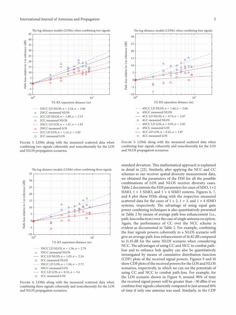
represent the SISO case and it is considered as a referencefor the quantitative analysis. Table 1 documents the resultantvalues of PLE and 𝜎 for all these schemes when consideringthe LOS and NLOS propagation scenarios. Figures 3, 4, and 5plot these LDMs with respect to 1m reference distance alongwith the respective measured scattered data for the cases of1 × 2, 1 × 3, and 1 × 4 SIMO systems, respectively.

The performance of CC over that of NCC is obvious inall these figures and is quantitatively documented in Table 1for each combining scheme. For instance, a reduction of55.98% is achieved if we combine four received powersnoncoherently in the LOS scenario, compared to 89.4%reduction in the same LOS scenario for the case of CCscheme. This performance superiority of CC over the NCCis already well established in the literature. It is also evidentfrom Table 1 that a significant reduction in the PLE can beachieved going from two receiving antenna elements to fourreceiving antennas, as expected.

4.2. Floating Intercept Path-Loss Models. The floating inter-cept path-loss model (FIM) is used in the 3GPP [17] andWINNER II [18] sets of standards, and it is given by [22]

PL (𝑑) [dB] = 𝛼 + 10𝛽 log10(𝑑) + 𝑋𝜎, (4)

where𝛼 is the floating intercept in dB and𝛽 is the linear slope.The parameters of this model are obtained by applying theleast-square linear regression fit to our measurement data inorder to find the best-fit values of 𝛼 and 𝛽 with minimum


The log-distance models (LDMs) when combining two signals

−10

−5

0

5

10

15

20

25

30

35

40

45

Path

-loss

relat

ive t

o 1 m

refe

renc

e (dB

)

101100

TX-RX separation distance (m)

2NCC measured NLOS

2NCC measured LOS

2CC measured NLOS

2CC measured LOS

2NCC LD NLOS, n = 2.24, = 3.66

2CC LD NLOS, n = 1.89, = 3.33

2NCC LD LOS, n = 1.47, = 1.92

2CC LD LOS, n = 1.14, = 2.02

Figure 3: LDMs along with the measured scattered data whencombining two signals coherently and noncoherently for the LOSand NLOS propagation scenarios.

−10

−5

0

5

10

15

20

25

30

35

Path

-loss

relat

ive t

o 1 m

refe

renc

e (dB

)

101100


3NCC measured NLOS

3NCC measured LOS

3CC measured NLOS

3CC measured LOS

3NCC LD NLOS, n = 1.56, = 2.79

3CC LD NLOS, n = 1.03, = 2.54

3NCC LD LOS, n = 1.04, = 2.72

3CC LD LOS, n = 0.52, = 3.4

The log-distance models (LDMs) when combining three signals

Figure 4: LDMs along with the measured scattered data whencombining three signals coherently and noncoherently for the LOSand NLOS propagation scenarios.

101100


4NCC measured NLOS

4NCC measured LOS

4CC measured NLOS

4CC measured LOS

4NCC LD NLOS, n = 1.44, = 2.66

4CC LD NLOS, n = 0.74, = 2.67

4NCC LD LOS, n = 0.93, = 2.85

4CC LD LOS, n = 0.22, = 3.87

The log-distance models (LDMs) when combining four signals

−10

−5

0

5

10

15

20

25

30

Path

-loss

relat

ive t

o 1 m

refe

renc

e (dB

)

Figure 5: LDMs along with the measured scattered data whencombining four signals coherently and noncoherently for the LOSand NLOS propagation scenarios.

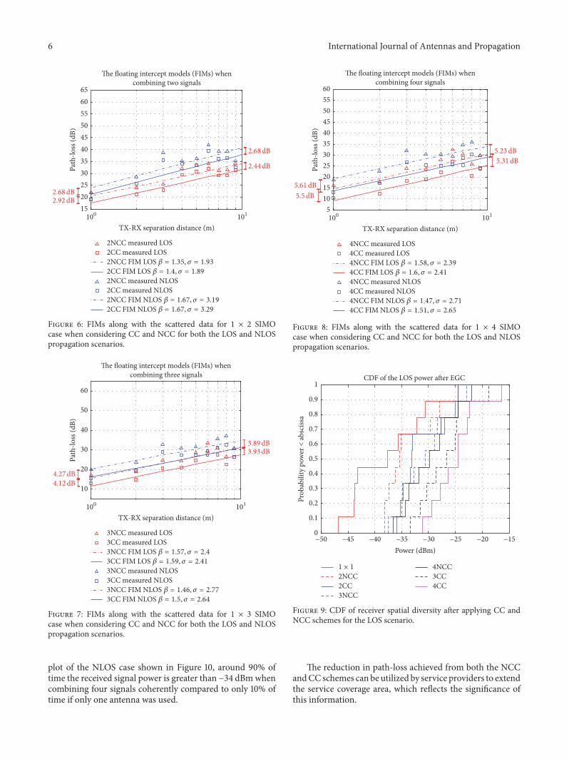
standard deviation.This mathematical approach is explainedin detail in [22]. Similarly, after applying the NCC and CCschemes to our receiver spatial diversity measurement data,we obtained the parameters of the FIM for all the possiblecombinations of LOS and NLOS receiver diversity cases.Table 2 documents the FIMparameters for cases of SISO, 1×2SIMO, 1 × 3 SIMO, and 1 × 4 SIMO systems. Figures 6, 7,and 8 plot these FIMs along with the respective measuredscattered data for the cases of 1 × 2, 1 × 3, and 1 × 4 SIMOsystems, respectively. The advantage of using equal gainpower combining techniques is also quantitatively presentedin Table 2 by means of average path-loss enhancement (i.e.,path-loss reduction) over the case of single antenna reception.Again, the performance of CC over the NCC scheme isevident as documented in Table 2. For example, combiningthe four signals powers coherently in a NLOS scenario willgive an average path-loss enhancement of 16.82 dB comparedto 11.45 dB for the same NLOS scenario when consideringNCC.The advantages of using CC and NCC to combat path-loss and to enhance link quality can also be quantitativelyinvestigated by means of cumulative distribution function(CDF) plots of the received signal powers. Figures 9 and 10showCDFplots of the received powers for the LOS andNLOSscenarios, respectively, in which we can see the potentials ofusing CC and NCC to combat path-loss. For example, forthe LOS scenario shown in Figure 9, around 90% of timethe received signal power will be greater than −30 dBm if wecombine four signals coherently compared to just around 10%of time if only one antenna was used. Similarly, in the CDF


The floating intercept models (FIMs) whencombining two signals

2.68 dB

2.44 dB

2.92 dB2.68 dB

2NCC measured LOS2CC measured LOS

2CC measured NLOS2NCC measured NLOS

2NCC FIM LOS = 1.35, = 1.93

2CC FIM NLOS = 1.67, = 3.29

2CC FIM LOS = 1.4, = 1.89

1520253035404550556065

Path

-loss

(dB)

101100


= 1.67, = 3.192NCC FIM NLOS

Figure 6: FIMs along with the scattered data for 1 × 2 SIMOcase when considering CC and NCC for both the LOS and NLOSpropagation scenarios.

The floating intercept models (FIMs) whencombining three signals

4.12 dB4.27 dB

3.89 dB3.93 dB


3CC measured NLOS3NCC measured NLOS

3NCC FIM LOS = 1.57, = 2.4

3CC FIM NLOS = 1.5, = 2.64

101100


10

20

30

40

50

60

Path

-loss

(dB)

= 1.59, = 2.413CC FIM LOS

= 1.46, = 2.773NCC FIM NLOS


plot of the NLOS case shown in Figure 10, around 90% oftime the received signal power is greater than −34 dBmwhencombining four signals coherently compared to only 10% oftime if only one antenna was used.

The floating intercept models (FIMs) whencombining four signals

5.31 dB5.23 dB

5.61 dB5.5 dB

101100


51015202530354045505560

Path

-loss

(dB)

4CC FIM NLOS = 1.51, = 2.65

4CC measured NLOS4NCC measured NLOS4CC FIM LOS = 1.6, = 2.41

4NCC FIM LOS = 1.58, = 2.39


= 1.47, = 2.714NCC FIM NLOS


CDF of the LOS power after EGC

2NCC2CC3NCC

4NCC3CC4CC

0

0.1

0.2

0.3

0.4

0.5

0.6

0.7

0.8

0.9

1

Prob

abili

ty p

ower

< ab

sciss

a

−15−40 −35 −30 −25 −20−45−50Power (dBm)

1 × 1

Figure 9: CDF of receiver spatial diversity after applying CC andNCC schemes for the LOS scenario.

The reduction in path-loss achieved from both the NCCandCC schemes can be utilized by service providers to extendthe service coverage area, which reflects the significance ofthis information.


Table 2: FIM parameters along with the average path-loss enhancements of receiver diversity for all the cases of SIMO reception.

Scenario LOS NLOSCombining type NCC CC NCC CCDiversity scheme 1 × 2 1 × 3 1 × 4 1 × 1 1 × 2 1 × 3 1 × 4 1 × 2 1 × 3 1 × 4 1 × 1 1 × 2 1 × 3 1 × 4𝛼 [dB] 21.42 16.53 15.57 24.75 18.5 12.41 10.07 24.83 21.26 20.26 31.36 22.15 16.99 14.65𝛽 1.35 1.57 1.58 1.54 1.4 1.59 1.6 1.67 1.46 1.47 1.53 1.67 1.5 1.51𝜎 [dB] 1.93 2.4 2.39 3.81 1.89 2.41 2.41 3.19 2.77 2.71 5.21 3.29 2.64 2.65Average enhancement in path-loss (dB) 4.52 8.08 8.98 — 7.11 12.06 14.34 5.6 10.53 11.45 — 8.32 14.56 16.82

CDF of the NLOS power after EGC

2NCC2CC3NCC

4NCC3CC4CC

−55 −50 −20−45 −35 −25−40 −30−60Power (dBm)

0

0.1

0.2

0.3

0.4

0.5

0.6

0.7

0.8

0.9

1

Prob

abili

ty p

ower

< ab

sciss

a

1 × 1

Figure 10: CDF of receiver spatial diversity after applying CC andNCC schemes for the NLOS scenario.

5. Receiver Spatial Diversity PropagationPath-Loss Channel Models

It was noticed that, at any TX-RX individual location, thepath-loss values are reduced in a logarithmic manner as thenumber of diversity antenna elements being combined goesfrom one up to four, for both the NCC and CC schemes.This is depicted in Figure 11, which shows the path-lossreduction at 8m separation distance for the NCC and CCschemes when considering the LOS propagation scenario.Furthermore, it is also evident from Figures 3–5 that theslope (or PLE) is reduced as a function of the number ofcombined signal powers. Therefore, we rely on these trendsobserved in our data to propose measurements-based spatialdiversity propagation path-loss channel models that accountfor the number of receiving diversity antennas in the path-loss equations. The proposed diversity models are developedbased on the log-distance path-loss model that is given by (3)and the floating intercept path-loss model that is given by (4).These models account for the number of antenna elementsdirectly in the path-loss estimation.

Path-loss reduction (CC)Path-loss reduction (NCC)

−5

0

5

10

15

20

Path

-loss

(dB)

32 2.5 3.51 41.5Number of combined signals

Figure 11: The logarithmic-like reduction in the path-loss values asthe number of diversity antennas goes from one up to four at 8mseparation distance for the LOS scenario.

The proposed log-distance-based diversity path-lossmodel is given by

PLDiv (𝑑) [dB] = PL (𝑑0) + (10𝑛SISOlog10 ( 𝑑𝑑0))⋅ (1 − 𝐴 log2(𝑁𝑟)) + 𝑋𝜎,

(5)

while the floating intercept-based diversity path-loss modelis given by

PLDiv (𝑑) [dB] = 𝛼SISO (1 − 𝐵 log2 (𝑁𝑟))+ 10𝛽SISOlog10 (𝑑) + 𝑋𝜎, (6)

where 𝑛SISO is the PLE for a single antenna reception (SISOscheme), 𝛼SISO is the floating intercept for the SISO case,𝛽SISO is the linear slope for the SISO case, 𝑁𝑟 is the numberof receiving diversity antenna elements, and 𝐴 and 𝐵 areweighting factors that are obtained by applying the MMSE fit(or least-square linear regression fit) to find the best-fit valueto the measured data with minimum standard deviation. Forthe log-distance-based diversity model, the values of 𝐴 areobtained by fixing the values of 𝑛SISO and then performing the


MMSE fit in order to find the best values of 𝐴 that give thecorresponding measured values of PL and 𝑁𝑟, whereas, forthe floating intercept-based diversity model, the respectivevalues of 𝐵 are determined by first fixing the values of 𝛼SISOand 𝛽SISO and then performing the MMSE fit to determinethe best values of 𝐵 that give the corresponding values ofPL and 𝑁𝑟. The closed-form expressions used to find 𝐴 and𝐵 along with their derivations are provided in Appendix.These approaches are used to obtain the values of 𝐴 and𝐵 for both diversity models for the CC and NCC schemeswhen considering LOS and NLOS propagation scenarios.Table 3 documents the values of𝐴 and𝐵 for the two proposeddiversity models that are given by (5) and (6). It is worthpointing out that the proposed diversity models given by (5)and (6) reduce to (3) and (4), respectively, when𝑁𝑟 = 1 (theSISO case), as would be required.

Next, we test the accuracy of the proposed diversitymodels to see how accurately they match the measured path-loss curves. Figures 12–15 compare the log-distance-baseddiversity path-loss model (5) with the measured log-distancemodel (3) for the CC and NCC when considering LOSpropagation scenario. Figures 12 and 13 present these resultsfor LOS scenarios for the CC and NCC, respectively, whileFigures 14 and 15 present these results for NLOS scenariosfor the CC and NCC, respectively. On the other hand, theaccuracy of the floating intercept-based diversity model (6)is examined by comparing it with the measured floatingintercept model (4). Figures 16–19 plot this diversity modelagainst the measured floating intercept models for the CCand NCC schemes when considering LOS scenario. Figures16 and 17 present these results for LOS scenario for the CCand NCC, respectively, while Figures 18 and 19 present theseresults for NLOS scenario for the CC and NCC, respectively.

It is evident from all these figures that the proposeddiversity path-loss models match the measured path-lossmodels fairly well for all the CC and NCC schemes whenconsidering the LOS and NLOS scenarios, after applying theappropriate values of the weighting factors 𝐴 and 𝐵.

The proposed receiver spatial diversity propagation path-loss models given by (5) and (6) are quite useful. This is dueto their ability to estimate or predict the path-loss valueseven for the case when we combine more than four signals(i.e., 𝑁𝑟 > 4), given that we are considering the samemeasurement parameters (i.e., carrier frequency, operatingenvironment, propagation scenario, and TX/RX heights). Allwhat one needs is to choose the appropriate values of diversitymodels’ parameters from Tables 1, 2, and 3 (i.e., 𝐴, 𝐵, 𝑛SISO,𝛼SISO, and 𝛽SISO) and the diversity models can estimate thepath-loss values for the case 𝑁𝑟 > 4. For example, usingthe floating intercept-based diversity model given by (6) onewould use 𝛼SISO = 31.36 and 𝛽SISO = 1.53 along with𝐵 = 0.276 from Tables 2 and 3, respectively, to estimatethe path-loss for NLOS CC case when combining 3, 5, 7,and 10 signals given that we have the same measurementparameters. Figure 20 shows the path-loss prediction forthis case. For the respective case but with using the log-distance-based diversity model given by (5), one would use𝑛SISO = 2.959 along with 𝐴 = 0.385 from Tables 1 and 3in which similar trends to those shown in Figure 20 would

Diversity model versus log-distance models (LDMs) for CC

−5

0

5

10

15

20

25

30

35

40

Path

-loss

relat

ive t

o 1 m

refe

renc

e (dB

)

101100


Diversity model 1 × 3

LDM 1 × 3


LDM 1 × 4


LDM 1 × 1

LDM 1 × 2


Figure 12: Path-loss for the proposed log-distance-based diversitymodel given by (5) for the CC scheme when considering LOSscenario, with 𝑛SISO = 2.105 and 𝐴 = 0.458.

Diversity model versus log-distance models (LDMs) for NCC

−5

0

5

10

15

20

25

30

35

40

Path

-loss

relat

ive t

o 1 m

refe

renc

e (dB

)

101100



LDM 1 × 3


LDM 1 × 4


LDM 1 × 1

LDM 1 × 2


Figure 13: Path-loss for the proposed log-distance-based diversitymodel given by (5) for the NCC scheme when considering LOSscenario, with 𝑛SISO = 2.105 and 𝐴 = 0.296.

be observed. Another advantage of the proposed generaldiversity path-loss models given by (5) and (6) is that theyrequire less number of parameters calculations for any arbi-trary number of coherently/noncoherently combined signals𝑁𝑟. For example, consider the case if we try to combinesixteen signals either coherently or noncoherently. Whenusing the floating intercept-based general diversitymodel (6),


Table 3: Parameters of the proposed receiver spatial diversity path-loss models presented in (5) and (6).

Diversity model Log-distance-based diversity model Floating intercept-based diversity modelScenario LOS NLOS LOS NLOSCombining scheme NCC CC and SISO NCC CC and SISO NCC CC and SISO NCC CC and SISO𝐴 0.296 0.458 0.269 0.385 — — — —𝐵 — — — — 0.189 0.295 0.192 0.276𝜎 [dB] 3.777 4.051 5.89 3.174 2.32 2.75 3 3.65

Diversity model versus log-distance models (LDMs) for CC

101100


−5

0

5

10

15

20

25

30

35

40

Path

-loss

relat

ive t

o 1 m

refe

renc

e (dB

)


LDM 1 × 3


LDM 1 × 4


LDM 1 × 1

LDM 1 × 2


Figure 14: Path-loss for the proposed log-distance-based diversitymodel given by (5) for the CC scheme when considering NLOSscenario, with 𝑛SISO = 2.959 and 𝐴 = 0.385.

Diversity model versus log-distance models (LDMs) for NCC

−5

0

5

10

15

20

25

30

35

40

Path

-loss

relat

ive t

o 1 m

refe

renc

e (dB

)

101100



LDM 1 × 3


LDM 1 × 4


LDM 1 × 1

LDM 1 × 2


Figure 15: Path-loss for the proposed log-distance-based diversitymodel given by (5) for the NCC scheme when considering NLOSscenario, with 𝑛SISO = 2.959 and 𝐴 = 0.269.

Diversity model versus floating intercept models(FIMs) for CC

5

10

15

20

25

30

35

40

45

50

55

60

Path

-loss

(dB)

101100





FIM 1 × 1

FIM 1 × 2

FIM 1 × 3

FIM 1 × 4


Figure 16: Path-loss for the proposed floating intercept-baseddiversity model given by (6) for the CC scheme when consideringLOS scenario, with 𝛼SISO = 24.75, 𝛽SISO = 1.54, and 𝐵 = 0.295.instead of calculating thirty-two parameters (sixteen for𝛼 and another sixteen for 𝛽) in the standard FIM, weonly require to calculate three parameters in the proposeddiversity model, which are 𝐵, 𝛼SISO, and 𝛽SISO. This meansthat the proposed diversity model is using only three valuesto replace thirty-two values with a very good accuracy in thepath-loss estimates as shown in Figures 16–19 for our case.For the respective case but with using the log-distance-baseddiversity model (5), we only require to find two parametersin the proposed diversity model, which are 𝐴 and 𝑛SISOinstead of finding sixteen values of the PLE in the standardlog-distance model. This means that the proposed diversitymodel is using only two values to replace sixteen valueswith a very good accuracy in the path-loss estimates asshown in Figures 12–15 for our case. The proposed receiverspatial diversity path-loss channel models can thus be used inmodern wireless systems to account for the general numberof receiving diversity antennas in the path-loss calculation.

6. Conclusion

In this paper we propose receiver spatial diversity propaga-tion path-loss channel models. These models are developed


Diversity model versus floating intercept models(FIMs) for NCC

10

15

20

25

30

35

40

45

50

55

60

Path

-loss

(dB)

101100





FIM 1 × 1

FIM 1 × 2

FIM 1 × 3

FIM 1 × 4


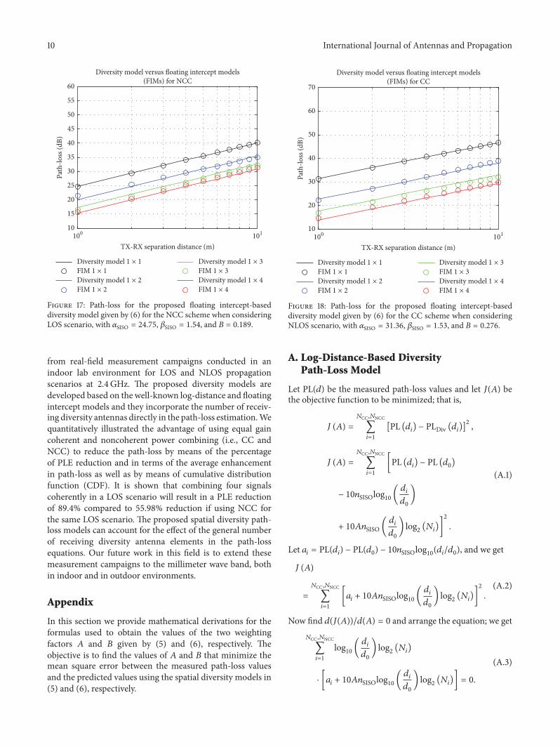
Figure 17: Path-loss for the proposed floating intercept-baseddiversity model given by (6) for the NCC scheme when consideringLOS scenario, with 𝛼SISO = 24.75, 𝛽SISO = 1.54, and 𝐵 = 0.189.

from real-field measurement campaigns conducted in anindoor lab environment for LOS and NLOS propagationscenarios at 2.4GHz. The proposed diversity models aredeveloped based on the well-known log-distance and floatingintercept models and they incorporate the number of receiv-ing diversity antennas directly in the path-loss estimation.Wequantitatively illustrated the advantage of using equal gaincoherent and noncoherent power combining (i.e., CC andNCC) to reduce the path-loss by means of the percentageof PLE reduction and in terms of the average enhancementin path-loss as well as by means of cumulative distributionfunction (CDF). It is shown that combining four signalscoherently in a LOS scenario will result in a PLE reductionof 89.4% compared to 55.98% reduction if using NCC forthe same LOS scenario. The proposed spatial diversity path-loss models can account for the effect of the general numberof receiving diversity antenna elements in the path-lossequations. Our future work in this field is to extend thesemeasurement campaigns to the millimeter wave band, bothin indoor and in outdoor environments.

Appendix

In this section we provide mathematical derivations for theformulas used to obtain the values of the two weightingfactors 𝐴 and 𝐵 given by (5) and (6), respectively. Theobjective is to find the values of 𝐴 and 𝐵 that minimize themean square error between the measured path-loss valuesand the predicted values using the spatial diversity models in(5) and (6), respectively.

Diversity model versus floating intercept models(FIMs) for CC

10

20

30

40

50

60

70

Path

-loss

(dB)

101100





FIM 1 × 1

FIM 1 × 2

FIM 1 × 3

FIM 1 × 4


Figure 18: Path-loss for the proposed floating intercept-baseddiversity model given by (6) for the CC scheme when consideringNLOS scenario, with 𝛼SISO = 31.36, 𝛽SISO = 1.53, and 𝐵 = 0.276.

A. Log-Distance-Based DiversityPath-Loss Model

Let PL(𝑑) be the measured path-loss values and let 𝐽(𝐴) bethe objective function to be minimized; that is,

𝐽 (𝐴) = 𝑁CC ,𝑁NCC∑𝑖=1

[PL (𝑑𝑖) − PLDiv (𝑑𝑖)]2 ,

𝐽 (𝐴) = 𝑁CC ,𝑁NCC∑𝑖=1

[PL (𝑑𝑖) − PL (𝑑0)− 10𝑛SISOlog10 ( 𝑑𝑖𝑑0)+ 10𝐴𝑛SISO ( 𝑑𝑖𝑑0) log2 (𝑁𝑖)]

2 .

(A.1)

Let 𝑎𝑖 = PL(𝑑𝑖) − PL(𝑑0) − 10𝑛SISOlog10(𝑑𝑖/𝑑0), and we get

𝐽 (𝐴)= 𝑁CC ,𝑁NCC∑𝑖=1

[𝑎𝑖 + 10𝐴𝑛SISOlog10 ( 𝑑𝑖𝑑0) log2 (𝑁𝑖)]2 . (A.2)

Now find 𝑑(𝐽(𝐴))/𝑑(𝐴) = 0 and arrange the equation; we get𝑁CC ,𝑁NCC∑𝑖=1

log10( 𝑑𝑖𝑑0) log2 (𝑁𝑖)

⋅ [𝑎𝑖 + 10𝐴𝑛SISOlog10 ( 𝑑𝑖𝑑0) log2 (𝑁𝑖)] = 0.(A.3)


Diversity model versus floating intercept models(FIMs) for NCC

10

20

30

40

50

60

70

Path

-loss

(dB)

101100



FIM 1 × 1

FIM 1 × 2



FIM 1 × 3

FIM 1 × 4


Figure 19: Path-loss for the proposed floating intercept-baseddiversity model given by (6) for the NCC scheme when consideringNLOS scenario, with 𝛼SISO = 31.36, 𝛽SISO = 1.53, and 𝐵 = 0.192.

Solving for 𝐴 we get the final formula as

𝐴= −∑𝑁CC ,𝑁NCC𝑖=1

log10(𝑑𝑖/𝑑0) log2 (𝑁𝑖) ∗ [𝑎𝑖]10𝑛SISO∑𝑁CC ,𝑁NCC𝑖=1(log10(𝑑𝑖/𝑑0))2 (log2 (𝑁𝑖))2 .

(A.4)

B. Floating Intercept-Based DiversityPath-Loss Model

Similarly,

𝐽 (𝐵) = 𝑁CC ,𝑁NCC∑𝑖=1

[PL (𝑑𝑖) − PLDiv (𝑑𝑖)]2 ,


[PL (𝑑𝑖) − 𝛼SISO + 𝐵𝛼SISOlog2 (𝑁𝑖)− 10𝛽SISOlog10 (𝑑𝑖)]2 .

(B.1)

Let 𝑎𝑖 = PL(𝑑𝑖) − 𝛼SISO − 10𝛽SISOlog10(𝑑𝑖), and we get


[𝑎𝑖 + 𝐵𝛼SISOlog2 (𝑁𝑖)]2 . (B.2)

Now find 𝑑(𝐽(𝐵))/𝑑(𝐵) = 0 and arrange the equation; we get

𝑁CC ,𝑁NCC∑𝑖=1

[𝑎𝑖log2 (𝑁𝑖) + 𝛼SISO𝐵 (log2 (𝑁𝑖))2] = 0. (B.3)

General diversity model after CC for the NLOS scenario

0

5

10

15

20

25

30

35

40

Path

-loss

(dB)

101100


General diversity modell (Nr = 3)

General diversity model (Nr = 5)



Figure 20: Path-loss prediction for arbitrary number of combinedsignals using the proposed general receiver diversity path-lossmodelgiven by (6), for the NLOS CC case with 𝛼SISO = 31.36 and 𝛽SISO =1.53 along with 𝐵 = 0.276 from Tables 2 and 3, respectively.

Solving for 𝐵 we get the final formula as

𝐵 = −∑𝑁CC ,𝑁NCC𝑖=1log2(𝑁𝑖) ∗ [𝑎𝑖]

𝛼SISO∑𝑁CC ,𝑁NCC𝑖=1(log2(𝑁𝑖))2 . (B.4)

Conflicts of Interest

The authors declare that they have no conflicts of interest.

Acknowledgments

The project was supported by King Saud University, Dean-ship of Scientific Research, College of Engineering ResearchCenter.

References

[1] T. S. Rappaport,Wireless Communications: Principles and Prac-tice, Prentice Hall, Upper Saddle River, NJ, USA, 2nd edition,2002.

[2] D. G. Brennan, “Linear diversity combining techniques,” Pro-ceedings of the IEEE, vol. 91, no. 2, pp. 331–356, 2003.

[3] A. I. Sulyman and M. Kousa, “Bit error rate performance of ageneralized diversity selection combining scheme in Nakagamifading channels,” in Proceedings of the IEEE Wireless Commu-nications and Networking Conference (WCNC ’00), vol. 3, pp.1080–1085, IEEE, September 2000.

[4] I. S. Ansari, F. Yilmaz, M.-S. Alouini, and O. Kucur, “Newresults on the sum of gamma random variates with applica-tion to the performance of wireless communication systems


over nakagami-m fading channels,” Transactions on EmergingTelecommunications Technologies, vol. 28, no. 1, Article ID e2912,2017.

[5] H. H. Beverage and H. O. Peterson, “Diversity receiving sys-tem of R.C.A. communications, inc., for radiotelegraphy,” Pro-ceedings of the Institute of Radio Engineers, vol. 19, no. 4, pp. 529–561, 1931.

[6] K. T. Herring, J. W. Holloway, D. H. Staelin, and D. W. Bliss,“Path-Loss characteristics of urban wireless channels,” IEEETransactions onAntennas andPropagation, vol. 58, no. 1, pp. 171–177, 2010.

[7] H. Kdouh, C. Brousseau, G. Zaharia, G. Grunfelder, and G.El Zein, “Measurements and path loss models for shipboardenvironments at 2.4GHz,” in Proceedings of the IEEE 201141st European Microwave Conference (EuMC ’11), pp. 408–411,October 2011.

[8] X. Zhao, B. M. Coulibaly, X. Liang et al., “Comparisons ofchannel parameters and models for urban microcells at 2 GHzand 5 GHz [wireless corner],” IEEE Antennas and PropagationMagazine, vol. 56, no. 6, pp. 260–276, 2014.

[9] V. Erceg, P. Soma, D. S. Baum, and S. Catreux, “Multiple-inputmultiple-output fixedwireless radio channelmeasurements andmodeling using dual-polarized antennas at 2.5 GHz,” IEEETransactions on Wireless Communications, vol. 3, no. 6, pp.2288–2298, 2004.

[10] Y.Wang, X.-L.Wang, Y.Qin, Y. Liu,W.-J. Lu, andH.-B. Zhu, “Anempirical path loss model in the indoor stairwell at 2.6 GHz,” inProceedings of the IEEE International Wireless Symposium (IWS’14), pp. 1–4, March 2014.

[11] J.-M. Molina-Garcıa-Pardo, J.-V. Rodrıguez, and L. Juan-Llacer,“Polarized indoor MIMO channel measurements at 2.45 GHz,”IEEE Transactions on Antennas and Propagation, vol. 56, no. 12,pp. 3818–3828, 2008.

[12] R. Mardeni and Y. Solahuddin, “Path loss model developmentfor indoor signal loss prediction at 2.4 GHz 802.11n network,” inProceedings of the International Conference on Microwave andMillimeter Wave Technology (ICMMT ’12), vol. 2, pp. 724–727,May 2012.

[13] S. Phaiboon, “Space diversity path loss in a modern factory atfrequency of 2.4 GHz,” WSEAS Transactions on Communica-tions, vol. 13, pp. 386–393, 2014.

[14] H.-G. Park, H. Keum, and H.-G. Ryu, “Path loss model withmultipleantenna,” in Proceedings of the Progress in Electromag-netics Research Symposium, pp. 2119–2124, Guangzhou, China,August 2014.

[15] A. Alwarafy, A. I. Sulyman, A. Alsanie, S. Alshebeili, andH. Behairy, “Receiver spatial diversity propagation path-lossmodel for an indoor environment at 2.4 GHz,” in Proceedings ofthe International Conference on the Network of the Future (NOF’15), pp. 1–4, October 2015.

[16] A. I. Sulyman, A. Alwarafy, G. R. MacCartney, T. S. Rappaport,andA.Alsanie, “Directional radio propagation path lossmodelsfor millimeter-wave wireless networks in the 28-, 60-, and 73-GHz bands,” IEEE Transactions on Wireless Communications,vol. 15, no. 10, pp. 6939–6947, 2016.

[17] V6.1.0, 3GPP TR 25.996, Spatial channel model for multipleinput multiple output MIMO simulations, September 2003.

[18] P. Kyosti, J. Meinila, L. Hentila et al., “D1. 1.2 WINNER II chan-nel models part I channel models,” Tech. Rep. IST-4-027756,WINNER Information Society Technologies, 2007.

[19] MangoCommunications, http://mangocomm.com/products/kits/warp-v3-kit.

[20] K. M. Humadi, A. I. Sulyman, and A. Alsanie, “Experimentalresults for generalized spatial modulation scheme with varia-ble active transmit antennas,” in Proceedings of the 10th Inter-national Conference on Cognitive Radio Oriented Wireless Net-works (IEEE-Crowncom ’15), Doha, Qatar, April 2015.

[21] A. Sulyman, A. Nassar, M. Samimi, G. Maccartney, T. Rappa-port, and A. Alsanie, “Radio propagation path loss models for5G cellular networks in the 28 GHZ and 38 GHZ millimeter-wave bands,” IEEE CommunicationsMagazine, vol. 52, no. 9, pp.78–86, 2014.

[22] J. F. Kenney and E. S. Keeping, Mathematics of Statistics, vanNostrand, Princeton, NJ, USA, 1965.

http://mangocomm.com/products/kits/warp-v3-kit

http://mangocomm.com/products/kits/warp-v3-kit

RoboticsJournal of

Hindawi Publishing Corporationhttp://www.hindawi.com Volume 2014


Active and Passive Electronic Components

Control Scienceand Engineering

Journal of


International Journal of

RotatingMachinery


Hindawi Publishing Corporation http://www.hindawi.com

Journal of

Volume 201

Submit your manuscripts athttps://www.hindawi.com

VLSI Design



Shock and Vibration


Civil EngineeringAdvances in

Acoustics and VibrationAdvances in



Electrical and Computer Engineering

Journal of

Advances inOptoElectronics

Hindawi Publishing Corporation http://www.hindawi.com

Volume 2014

The Scientific World JournalHindawi Publishing Corporation http://www.hindawi.com Volume 2014

SensorsJournal of


Modelling & Simulation in EngineeringHindawi Publishing Corporation http://www.hindawi.com Volume 2014


Chemical EngineeringInternational Journal of Antennas and

Propagation




Navigation and Observation



DistributedSensor Networks


path-loss channel models for receiver spatial diversity...

Documents