i

Pasture Phosphorus Management(PPM) Calculator

Technical DocumentationVersion 1.0

Michael White & Daniel Storm Tesfaye Demissie

Biosystems and Agricultural Engineering Department

Hailin ZhangPlant and Soil Sciences Department

Michael SmolenBiosystems and Agricultural Engineering Department

Division of Agricultural and Natural ResourcesOklahoma State University

December 31, 2003

ii

AcknowledgmentsThe authors and developers of the PPM Calculator would like to acknowledge the contribution ofthe Soil and Water Assessment Tool team (Grassland, Soil and Water Research Laboratory,USDA-ARS), in particular Dr. Jeff Arnold, for their support in the development of this tool. We wouldalso like to thank Dr. Daren Redfern for his contribution to the forage and grazing management partof the program. This work was supported in part by the Oklahoma Agricultural Experiment Stationand Oklahoma Cooperative Extension Service.

iii

Table of ContentsExecutive Summary . . . . . . . . . . . . . . . . . . . . . . . . . . . . . . . . . . . . . . . . . . . . . . . . . . . . . . . . . . 1

Introduction and Background . . . . . . . . . . . . . . . . . . . . . . . . . . . . . . . . . . . . . . . . . . . . . . . . . . . 3

SWAT 2000 Background . . . . . . . . . . . . . . . . . . . . . . . . . . . . . . . . . . . . . . . . . . . . . . . . . . . . . . 4

PPM Calculator Model Components . . . . . . . . . . . . . . . . . . . . . . . . . . . . . . . . . . . . . . . . . . . . . 5

PPM Calculator User Interface . . . . . . . . . . . . . . . . . . . . . . . . . . . . . . . . . . . . . . . . . . . . . . . . . . 5Input Parameters . . . . . . . . . . . . . . . . . . . . . . . . . . . . . . . . . . . . . . . . . . . . . . . . . . . . . . 5Buttons . . . . . . . . . . . . . . . . . . . . . . . . . . . . . . . . . . . . . . . . . . . . . . . . . . . . . . . . . . . . . . 7Output . . . . . . . . . . . . . . . . . . . . . . . . . . . . . . . . . . . . . . . . . . . . . . . . . . . . . . . . . . . . . . . 8Quality Assurance and Quality Control Features . . . . . . . . . . . . . . . . . . . . . . . . . . . . . . 9

SWAT Input Parameters . . . . . . . . . . . . . . . . . . . . . . . . . . . . . . . . . . . . . . . . . . . . . . . . . . . . . . . 9HRU Properties (.HRU) . . . . . . . . . . . . . . . . . . . . . . . . . . . . . . . . . . . . . . . . . . . . . . . . . 9Soil Chemistry File (.CHM) . . . . . . . . . . . . . . . . . . . . . . . . . . . . . . . . . . . . . . . . . . . . . . 10

Correcting STP for Differences in Laboratory Methods . . . . . . . . . . . . . . . . . . 10Relating Soil Test Phosphorous to SWAT Soil Labile Phosphorus . . . . . . . . . 11

Soil Properties (.SOL) . . . . . . . . . . . . . . . . . . . . . . . . . . . . . . . . . . . . . . . . . . . . . . . . . . 11Management Operations (.MGT) . . . . . . . . . . . . . . . . . . . . . . . . . . . . . . . . . . . . . . . . . 12

General Management Variables . . . . . . . . . . . . . . . . . . . . . . . . . . . . . . . . . . . . 12Minimum Dry Biomass (BIOMIN) . . . . . . . . . . . . . . . . . . . . . . . . . . . . . 12Curve Number . . . . . . . . . . . . . . . . . . . . . . . . . . . . . . . . . . . . . . . . . . . . 12General Management Default Variables . . . . . . . . . . . . . . . . . . . . . . . . 12

Management Operations . . . . . . . . . . . . . . . . . . . . . . . . . . . . . . . . . . . . . . . . . 13Plant/Begin Growing Season . . . . . . . . . . . . . . . . . . . . . . . . . . . . . . . . 13Fertilizer Application . . . . . . . . . . . . . . . . . . . . . . . . . . . . . . . . . . . . . . . 13Hay . . . . . . . . . . . . . . . . . . . . . . . . . . . . . . . . . . . . . . . . . . . . . . . . . . . . 13Grazing . . . . . . . . . . . . . . . . . . . . . . . . . . . . . . . . . . . . . . . . . . . . . . . . . 13

Basin Configuration (.BSN) . . . . . . . . . . . . . . . . . . . . . . . . . . . . . . . . . . . . . . . . 13Eucha Calibration Parameters . . . . . . . . . . . . . . . . . . . . . . . . . . . . . . . . . . . . . . . . . . . 14

PPM Calculator Verification and Sensitivity Analysis . . . . . . . . . . . . . . . . . . . . . . . . . . . . . . . . 14

PPM Calculator Validation . . . . . . . . . . . . . . . . . . . . . . . . . . . . . . . . . . . . . . . . . . . . . . . . . . . . 19

Limitations . . . . . . . . . . . . . . . . . . . . . . . . . . . . . . . . . . . . . . . . . . . . . . . . . . . . . . . . . . . . . . . . 23

Proposed Future Work . . . . . . . . . . . . . . . . . . . . . . . . . . . . . . . . . . . . . . . . . . . . . . . . . . . . . . . 23

References . . . . . . . . . . . . . . . . . . . . . . . . . . . . . . . . . . . . . . . . . . . . . . . . . . . . . . . . . . . . . . . . 25

Appendix . . . . . . . . . . . . . . . . . . . . . . . . . . . . . . . . . . . . . . . . . . . . . . . . . . . . . . . . . . . . . . . . . . 27Appendix A

SWAT Peer Reviewed Publications . . . . . . . . . . . . . . . . . . . . . . . . . . . . . . . . . 28Appendix B

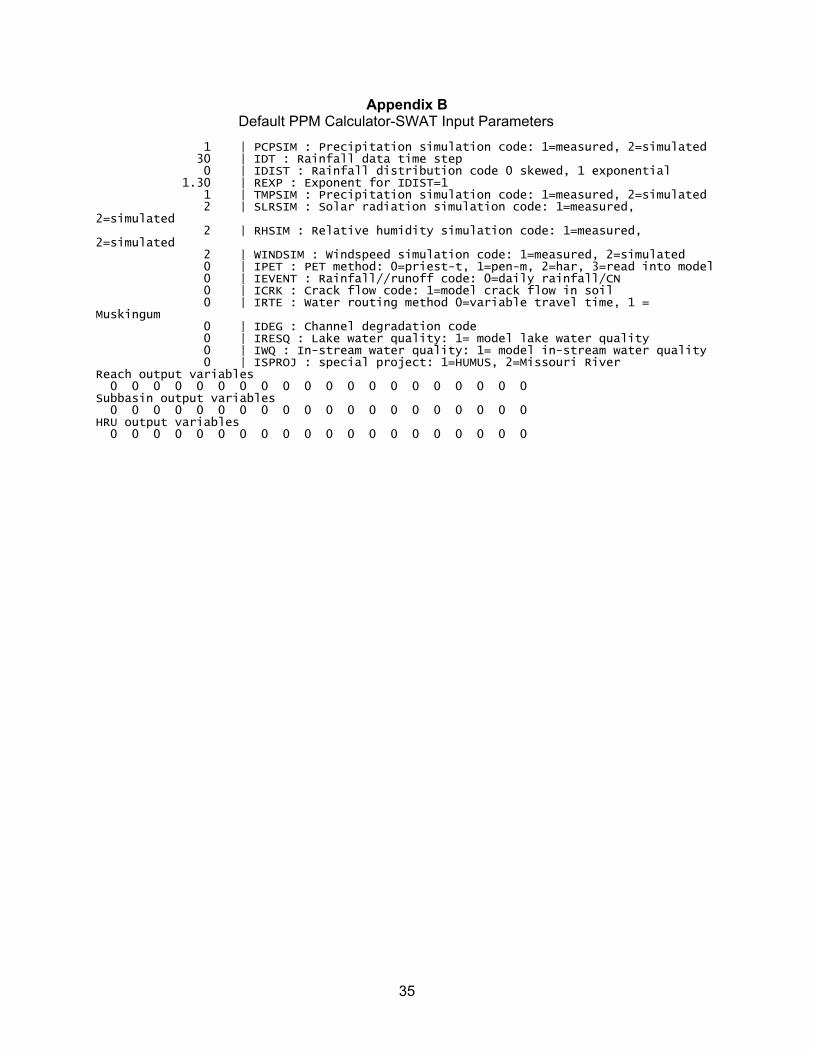
Default PPM Calculator-SWAT Input Parameters . . . . . . . . . . . . . . . . . . . . . . 33

iv

Appendix CRelationship between Oklahoma State University and University ofArkansas Soil Test Phosphorus . . . . . . . . . . . . . . . . . . . . . . . . . . . . . . . . . . . . 36

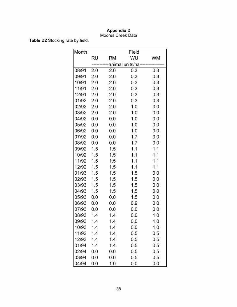
Appendix DMoores Creek Data . . . . . . . . . . . . . . . . . . . . . . . . . . . . . . . . . . . . . . . . . . . . . . 37

Appendix EGraphical Verification Results . . . . . . . . . . . . . . . . . . . . . . . . . . . . . . . . . . . . . . 39

1

Executive SummaryIn December of 2001 the City of Tulsa and the Tulsa Metropolitan Utility Authority filed suit inFederal Court against Tyson Foods, Inc., Cobb-Vantress Inc., Peterson Farms, Inc., SimmonsFoods, Inc., Cargill, Inc., George’s, Inc., and the City of Decatur, Arkansas for damages andinjunctive relief for one of the City of Tulsa’s water supplies, the Lake Eucha/Spavinaw complex(United States District Court for the Northern District of Oklahoma, Case No. 01 CV 0900EA[C]).In July of 2003 a settlement agreement between the parties was reached. The settlementagreement requested that Oklahoma State University and the University of Arkansas work on a“Phosphorus Risk Index” to be submitted to the Court by January 1, 2004. The technicalPhosphorus Index Team members of Oklahoma State University and the University of Arkansaswere unable to agree on a common Phosphorus Index, and thus Oklahoma State University issubmitting its own Phosphorus Index to the Court. The submitted Phosphorus Index meets therequirements of the settlement agreement and is specific to the Lake Eucha/Spavinaw basin.Presented is a technical document which describes the development, verification, sensitivityanalysis, and validation of the submitted Phosphorus Index.

The Phosphorus Index submitted to the Court and documented in this report is called the PasturePhosphorus Management (PPM) Calculator, which was developed at Oklahoma State UniversityDivision of Agricultural Sciences and Natural Resources by faculty and staff in the Biosystems andAgricultural Engineering and Plant and Soil Sciences Departments. The PPM Calculator is aquantitative tool developed to predict edge-of-field phosphorus loss from pasture systems in theLake Eucha/Spavinaw basin. The PPM Calculator is a simple interface written in Visual Basic thatuses the Soil and Water Assessment Tool (SWAT) 2000 model, which allows field personnel to takeadvantage of the predictive capacity of SWAT typically reserved for use by hydrologists andengineers. The PPM Calculator was designed to be simple to use by field personnel with readilyavailable inputs, and thus insulates the user from the complexity of SWAT by formatting modelinputs and interpreting model output. By using the physically based SWAT model, the PPMCalculator can accurately simulate a variety of management options under a variety of fieldconditions.

SWAT is a widely accepted model which has been used extensively by hydrologists and engineerssince 1994 in the United States as well as a number of other countries around the world. SWAT’sstrength lies in the physical basis of the model, which gives it the ability to make accuratepredications under a wide range of conditions and Best Management Practices (BMPs). The PPMCalculator only utilizes the “field” components of the SWAT model and does not use the channelrouting and transformation routines that may be needed when applying the model at a basin scale.

The PPM Calculator was designed to prevent the model from being modified by a user and therebyproduce incorrect results. The PPM Calculator requires several files to operate properly, and thusa modified or corrupt file may invalidate results generated by the model. Therefore, modification ofany file required by the PPM Calculator deactivates the software, forcing the user to reinstall thesoftware. The PPM Calculator also has smart input fields which help the user avoid mistakes. Allvalues entered in the interface are checked to ensure that they are numeric, positive and in theacceptable range for that parameter. Moving the cursor slowly over an input field will produce a tagwith information or guidance concerning that input. Various warnings and messages alert the userto possible mistakes. When possible, references tables or calculators are included to aid the user.Tools for estimating stocking rates in animal units, minimum available forage in dry weight, andfertilizer application rates are included.

To add to the reliability of the PPM Calculator, the model was verified for various parameters (or

2

processes), a sensitivity analysis was performed, and the model was validated. Verification is aprocess that certifies that the model components are working correctly. A sensitivity analysis is aprocess of identifying parameters that have the greatest impact on model output, and validation isa process that assures that the model functions properly and produces reasonable results underspecific conditions. The PPM Calculator was validated using 33 months of data on four fields justsouth of the Lake Eucha/Spavinaw basin using data presented by Edwards et al. (1994), Edwardset al. (1996a, 1996b), and Edwards et al. (1997). The validation process tests the PPM Calculatorwith observed data that is not used in calibration. The PPM Calculator was not directly calibrated;however the model made use of SWAT hydrologic parameters calibrated specifically for the LakeEucha/Spavinaw basin (Storm et al., 2003). Using these basin specific parameters significantlyincreases the reliability of the PPM Calculator when applied to pastures in the Eucha/Spavinawbasin. The performance of the PPM Calculator on the validation data set was excellent, thusproviding additional confidence in the model’s accuracy and predictive capability.

The PPM Calculator predicts average monthly and annual phosphorus loads based on 15 yearsof observed weather data. The PPM Calculator utilizes existing and proven technology and canbe used to determine the amount of litter that can be applied to a pasture to meet a specific waterquality objective. The PPM Calculator also allows the agricultural producer to select from a numberof management options that will minimize phosphorus loss from his/her field. Therefore, the PPMCalculator is an important component of an environmentally sound nutrient management plan.Another benefit of the PPM Calculator is that the nutrient management plan developer can workwith the agricultural producer on site to evaluate multiple management options in a few minutes anddevelop a plan that minimizes phosphorus loss as well as optimizing agricultural productivity.

The PPM Calculator is a physically-based quantitative tool based on a widely tested and acceptedmodel. A qualitative Phosphorus Index is less likely to accurately predict phosphorus lossespecially for conditions outside the range used to develop the index, and therefore it is unlikely thatone can accurately predict whether a specific water quality objective can be met. In order toaccurately predict phosphorus loss from a pasture system, the effects of the amount and timing ofgrazing, haying, and fertilization must be accounted for in a physically based hydrologic model. Itshould be noted that both a quantitative and qualitative Phosphorus Index require the selection ofa water quality endpoint (water quality objective). Although an endpoint is not required to run thePPM Calculator, the endpoint is required to determine the allowable phosphorus load allocation forpasture systems in the Lake Eucha/Spavinaw basin. A similar endpoint is required to setthresholds for a qualitative Phosphorus Index.

3

Introduction and BackgroundIn December of 2001 the City of Tulsa and the Tulsa Metropolitan Utility Authority filed suit inFederal Court against Tyson Foods, Inc., Cobb-Vantress Inc., Peterson Farms, Inc., SimmonsFoods, Inc., Cargill, Inc., George’s, Inc., and the City of Decatur, Arkansas for damages andinjunctive relief for one of the City of Tulsa’s water supplies, the Lake Eucha/Spavinaw complex(United States District Court for the Northern District of Oklahoma, Case No. 01 CV 0900EA[C]).In July of 2003 a settlement agreement between the parties was reached. The following is anexcerpt from the settlement agreement describing the intent of the settlement:

“C. STATEMENT OF INTENT....(2) to ensure that nutrient management protocolsare used in the Watershed to reduce the risk of harm to Plaintiffs’ Water Supply dueto the Land Application of Nutrients and The City of Decatur’s WWTP discharge,while at the same time recognizing the right of the Poultry Defendants and theirGrowers to continue to conduct poultry operations in the Watershed within suchprotocols and the importance of clean lakes, safe drinking water and a viable poultryindustry to the economics of Northeast Oklahoma and Northwest Arkansas.”

The settlement agreement also requested that Oklahoma State University and the University ofArkansas work on a “Phosphorus Risk Index” to be submitted to the Court by January 1, 2004.Below are excerpts from the settlement that describe the requested Phosphorus Index:

“17. “PI” means the risk based Phosphorus Index developed to govern the termsand conditions under which Nutrients may be land applied in the Watershed, asfurther described in Section D of this Agreement, and includes the numerical indexsystem represented thereby, the target objective or index necessary to limit the landapplication of Nutrients, as described therein, and any other associatedrequirements, limits or guidelines pertaining to the land application of Nutrients asprescribed by the PI developers. Page 2

1. A new phosphorus risk-based index (“PI”) shall be developed to govern the termsand conditions under which any Nutrients may be land applied in the Watershed.Although the PI, as developed or with modification, may have broader applicationor be of interest to other watersheds or parties not involved in the Watershed, thePI shall be developed particularly for the existing physical, geological andhydrological conditions and characteristics of the Watershed and the stated goalsand intent of this Agreement.

2. The PI shall be developed to achieve the least amount of total phosphorusreasonably attainable from each Application Site to the Water Supply from allsources of phosphorus on each such Application Site while still meeting theagronomic requirements for the growth of grasses, crops and other desirable plantlife.”

As part of the Settlement agreement, there is a moratorium on litter application in the basin “...untila Nutrient management Plan containing a PI number for each tract, field or pasture” is developed.The technical Phosphorus Index team members of Oklahoma State University and the Universityof Arkansas were unable to agree on a common Phosphorus Index, and thus Oklahoma StateUniversity is submitting its own Phosphorus Index to the Court. Presented is a technical documentwhich describes the development, verification, sensitivity analysis, and validation of the submittedindex. In its current form this Phosphorus Index should only be applied to pastures in the Lake

4

Figure 1. Lake Eucha/Spavinaw basin.

Eucha/Spavinaw basin.

The Lake Eucha/Spavinaw basin (Figure 1) islocated in northeast Oklahoma and northwestArkansas, and covers approximately 265,000acres of Delaware County, Oklahoma andBenton County, Arkansas. The basin is locatedin the Ozark Highlands and the CentralIrregular Plains Ecoregion. The land cover isprimarily pasture and forest. Forests are mostlydeciduous, but pine trees are common.Pastures are used for hay and grazing cattle.There are approximately 85 million chickensand turkeys produced annually in over 1000poultry houses in the basin, and thus poultrylitter is often applied to these pastures toincrease their productivity. The topography isKarst, with exposed limestone in some areas.Soils are mainly of the ultisol order, and are typically thin and highly permeable. Average annualprecipitation is approximately 45 inches. Additional details on the basin are given in Storm et al.(2002).

The Phosphorus Index submitted to the Court and documented in this report is called the PasturePhosphorus Management (PPM) Calculator, which was developed at the Oklahoma StateUniversity Division of Agricultural Sciences and Natural Resources by faculty and staff in theBiosystems and Agricultural Engineering and Plant and Soil Sciences Departments. The PPMCalculator was developed to predict phosphorus loss from pasture systems in the LakeEucha/Spavinaw basin. The PPM Calculator is a simple interface written in Visual Basic that usesthe Soil and Water Assessment Tool (SWAT) 2000 model, which allows field personnel to takeadvantage of the predictive capacity of SWAT typically reserved for use by hydrologists andengineers.

The PPM Calculator is a quantitative tool that predicts the edge-of-field average annual totalphosphorus load from pastures under a variety of management options. The PPM Calculator wasdesigned to be simple to use by field personnel, with readily available inputs. The PPM Calculatorinsulates the user from the complexity of SWAT by generating model inputs and interpreting modeloutput. By using the physically based SWAT model, the PPM Calculator can accurately simulatea variety of management practices and field characteristics.

SWAT 2000 BackgroundSWAT is a distributed parameter basin-scale model developed by the USDA Agricultural ResearchService at the Grassland, Soil and Water Research Laboratory in Temple, Texas. SWAT is includedin the Environmental Protection Agency’s (EPA) latest release of Better Assessment ScienceIntegrating Point and Nonpoint Sources (BASINS). The model has been used extensively undera variety of conditions in the United States as well as a number of other countries around the world.Additional documentation (Users Manual and Theoretical Documentation) for the SWAT model arelocated online at http://www.brc.tamus.edu/swat/swatdoc.html. A list of peer reviewed SWATpublications is given in Appendix A.

5

SWAT 2000 Input Files

PPM Calculator

SWAT 2000 Executable

SWAT 2000 Output Files

User (Field Staff)

Calibrated Eucha/SpavinawSWAT Model

PPM Calculator Model ComponentsThe PPM Calculator acts as an interface for the SWAT 2000 model while greatly simplifying its usefor modeling pasture systems. SWAT is a widely accepted model which has been used extensivelyby hydrologists and engineers since 1994 in the United States as well as a number of othercountries around the world. SWAT’s strength lies in the physical basis of the model, which givesit the ability to make accurate predications under a wide variety of Best Management Practices(BMPs). The PPM Calculator interacts with SWAT as shown in Figure 2. SWAT input files aregenerated using input from the user via the PPM Calculator interface and then used during theexecution of the model. The PPM Calculator summarizes the SWAT model output in a simple tablethat is easy to interpret. It should be noted that the PPM Calculator only utilizes the “field”components of the SWAT model and does not use the channel routing and transformation routinesthat may be needed when applying the model at a basin scale.

Figure 2. PPM Calculator block diagram.

PPM Calculator User InterfaceThe PPM Calculator user interface is the bridge between the user and the SWAT model. The userinterface is the only portion that the user interacts with. It was designed to be easy to use, but werecommend that users read the SWAT users manual. The PPM Calculator includes criticalreference tables and calculators to minimize the need for additional documents or software.

Input Parameters

The default PPM Calculator input parameters are given in Appendix B. The PPM Calculatorinterface (Figure 3) allows the user to specify the following parameters:

Field Owner - Owner or manager responsible for the property.

Plan Developer - Person who runs the PPM Calculator to develop a nutrient management plan fora particular field.

Field Description (optional) - Allows owners of multiple fields to add a description or name.

Date - Date plan is developed.

Field Area - Area of field not including buffer strips in acres.

Soil Type - The Interface contains data for 35 soils commonly found in the Eucha/Spavinaw basin.

6

Forage Type - Allows the user to select warm, cool, or mixed forages.

STP - Input for Mehlich III Soil Test Phosphorus. User must specify which lab performed theanalysis. All Soil Test Phosphorus measurements are converted to an Oklahoma State Universityequivalent.

Minimum Dry Forage - The minimum dry forage present on the field at any time of the year.Grazing is suspended by the program when this level is reached.

Forage Yield Goal - Used to calculate maximum nitrogen recommendations based on OSUguidelines. The program will alert the user if the nitrogen amount is exceeded.

Field Slope - The average field slope in percent.

Slope Length - Revised Universal Soil Loss Equation Slope Length in feet.

Slope to Stream (Not active in Version 1.0) - Average slope of the area between the field andnearest stream or concentrated flow channel.

Distance to Stream (Not active in Version 1.0) - Distance from field to nearest stream orconcentrated flow channel.

Alum Treated Litter (Not active in Version 1.0) - Used to indicate that litter is treated with alumbefore it is applied to a pasture, which may reduce soluble phosphorus loss.

Buffer Strip Width (Not active in Version 1.0) - Buffer strips are a BMP that may trap sediment andnutrients before they leave the field.

Field Center (UTM Coordinates) - Location of field being analyzed. These data are saved by PPMCalculator, but are not used in any calculations.

Hay - Used to indicate that a hay operation occurs this month. All operations are scheduled for thefirst day of the month selected.

Stocking Rate - Number of animal units per acre grazed each month. One animal unit is equivalentto a 1000 lb cow. The conversion table for other animal types is included in the PPM calculator.

Litter N - Total amount of nitrogen (as N) applied in litter this month.

Litter P - Total amount of phosphorus (as P2O5) applied in litter this month.

Commercial N - Amount of nitrogen (as N) applied in commercial fertilizers this month.

Commercial P - Amount of phosphorus (as P2O5) applied in commercial fertilizers this month.

Status and Warnings - This display shows the status of the program and displays warnings thatmay require corrective action by the user.

P Allocation - This is the maximum allowable phosphorus load permitted from pastures in theEucha/Spavinaw basin to meet a specific water quality objective. This endpoint must be set by theparties and/or the Court if the risk of P loss from a particular field is desired. The default value is

7

arbitrarily set to zero. This value is not required to run the PPM Calculator.

Buttons

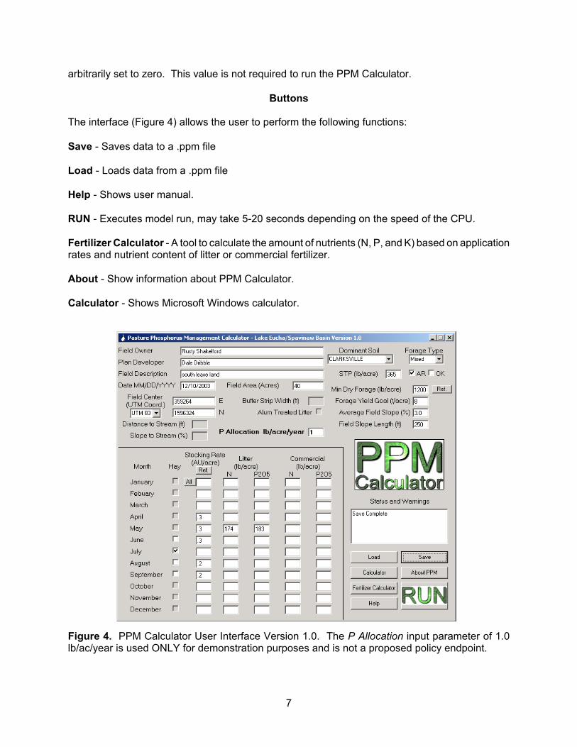
The interface (Figure 4) allows the user to perform the following functions:

Save - Saves data to a .ppm file

Load - Loads data from a .ppm file

Help - Shows user manual.

RUN - Executes model run, may take 5-20 seconds depending on the speed of the CPU.

Fertilizer Calculator - A tool to calculate the amount of nutrients (N, P, and K) based on applicationrates and nutrient content of litter or commercial fertilizer.

About - Show information about PPM Calculator.

Calculator - Shows Microsoft Windows calculator.

Figure 4. PPM Calculator User Interface Version 1.0. The P Allocation input parameter of 1.0lb/ac/year is used ONLY for demonstration purposes and is not a proposed policy endpoint.

8

Output

Output from the PPM Calculator is a standard .txt file witch can be read by any word processor ortext editor. All the information entered by the user is listed in the output, along with monthly andannual precipitation, runoff, sediment, total phosphorus, and estimated available forage. A messageat the bottom of the output tells the user if this scenario is predicted to meet the Parties and/orCourt specified Phosphorus Allocation.

Created 12/19/2003 1:36:43 PM by PPM Calculator 1.0

Field Owner: Rusty ShakelfordPlan Developer: Dale DribbleField Description: south lease landPlan Date: 12/10/2003Field Area (acres): 40Field Slope (%): 3.0Soil Type: CLARKSVILLE Hydrologic Group BCurve Number: 56Forage Type: MixedArkansas STP (lb/acre): 365 (OK Equivalent): 407Minimum Standing Forage (lb/acre): 1200Forage Yield Goal (ton/acre): 8UTM Coordinates: 359264E 1596324N UTM 83Allowed P Allocation (lb/acre/year): 1Hay Harvested (ton/acre/year): 2.2969

Month Hay Stocking Litter Commercial Precip Runoff Sediment Total Available Rate N P2O5 N P2O5 Phosphorus Forage (AU/acre) ----(Lb/acre)---- (in) (in) (t/acre) (lb/acre) (Dry ton/acre)

Jan 0.0 0 0 0 0 1.56 0.21 0.000 0.08 0.16 Feb 0.0 0 0 0 0 2.19 0.44 0.000 0.16 0.22 Mar 0.0 0 0 0 0 3.88 0.55 0.000 0.19 0.39 Apr 0.3 0 0 0 0 3.87 0.63 0.000 0.22 0.48 May 0.3 174 183 0 0 4.65 0.35 0.000 0.14 1.18 Jun 0.3 0 0 0 0 4.37 0.43 0.000 0.19 2.28 Jly X 0.0 0 0 0 0 2.64 0.04 0.000 0.02 1.02 Aug 0.2 0 0 0 0 3.77 0.07 0.000 0.03 1.90 Sep 0.2 0 0 0 0 3.34 0.18 0.000 0.08 2.68 Oct 0.0 0 0 0 0 3.67 0.20 0.000 0.09 3.30 Nov 0.0 0 0 0 0 3.87 0.33 0.000 0.14 0.17 Dec 0.0 0 0 0 0 2.45 0.37 0.000 0.16 0.17 ------------------------------------------------------------------------------------Annual Totals 174 183 0 0 40.26 3.80 0.002 1.48 WARNING: PPM Calculator predicts this management scenario will exceedthe allowable phosphorus load by 48.1%

NOTE: The P Allocation input parameter of 1.0 lb/ac/year is used ONLY for demonstration purposesand is not a proposed policy endpoint.

9

Quality Assurance and Quality Control Features

Smart InputsThe PPM Calculator has smart input fields which help the user avoid mistakes. All values enteredin the interface are checked to ensure that they are numeric, positive, and in the acceptable rangefor that parameter. Moving the cursor slowly over an input field will produce a tag with someinformation or guidance concerning that input. Various warnings and messages alert the user topossible mistakes. When possible, references tables or calculators are included to aid the user.Tools for estimating stocking rates in animal units, minimum available forage in dry weight, andfertilizer application rates are included.

Tamper ResistanceThe PPM Calculator requires several files to operate properly, these files are accessible to the userfor inspection only. A modified or corrupt file may invalidate results generated by the model.Therefore, modification of any file required by the PPM Calculator will deactivate the software,forcing the user to reinstall the program. The PPM Calculator was designed to prevent the modelfrom being modified and produce erroneous results.

SWAT Input Parameters

The PPM Calculator generates several files needed to run SWAT using site specific data providedby the user. Data entered by the user is transformed into a suitable format to be used by the SWATmodel. Files modified or created by the PPM Calculator are listed below:

HRU Properties (.HRU)Soil Chemistry File (.CHM)Soil Properties (.SOL)Management Operations (.MGT)Basin Configuration (.BSN)

The remaining SWAT files are not altered by the PPM Calculator. Parameters in these remainingfiles may be predefined SWAT defaults or taken directly from the SWAT model calibrated for theLake Eucha basin (Storm et al., 2003). The hydrologic parameters from the Lake Eucha/SpavinawSWAT model were used in the PPM Calculator (Storm et al., 2003). All files required to run SWATare visible in the \BIN directory of the PPM Calculator installation. These can be inspected at anytime by any user; however if any file is corrupted or modified the PPM Calculator will not run, andreinstallation will be required.

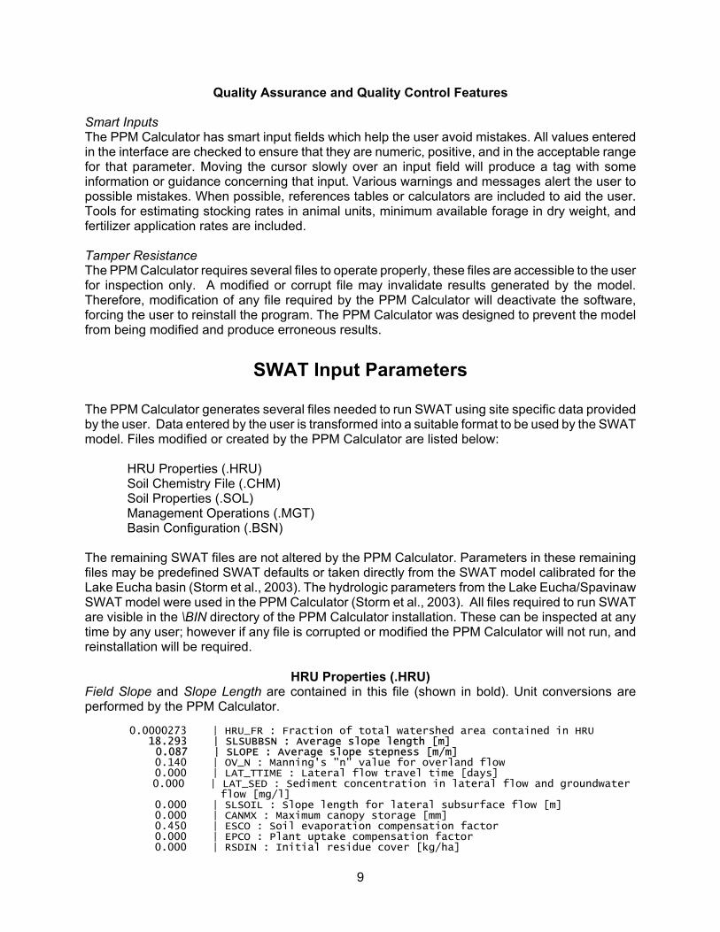
HRU Properties (.HRU)Field Slope and Slope Length are contained in this file (shown in bold). Unit conversions areperformed by the PPM Calculator.

0.0000273 | HRU_FR : Fraction of total watershed area contained in HRU 18.293 | SLSUBBSN : Average slope length [m] 0.087 | SLOPE : Average slope stepness [m/m] 0.140 | OV_N : Manning's "n" value for overland flow 0.000 | LAT_TTIME : Lateral flow travel time [days]

0.000 | LAT_SED : Sediment concentration in lateral flow and groundwater flow [mg/l]

0.000 | SLSOIL : Slope length for lateral subsurface flow [m] 0.000 | CANMX : Maximum canopy storage [mm] 0.450 | ESCO : Soil evaporation compensation factor 0.000 | EPCO : Plant uptake compensation factor 0.000 | RSDIN : Initial residue cover [kg/ha]

10

0.000 | ERORGN : Organic N enrichment ratio 0.000 | ERORGP : Organic P enrichment ratio 0.000 | FILTERW : Filter strip width 0 | IURBAN : Urban simulation code 0 | URBLU : Urban land type identification number 0 | IRR : Irrigation code 0 | IRRNO : Irrigation source location 0.000 | FLOWMIN : Minimum in-stream flow for irrigation 0.000 | DIVMAX : Maximum daily irrigation diversion from the reach [mm] 0.000 | FLOWFR : Fraction of available flow 0.000 | DDRAIN : Depth to surface drain [mm] 0.000 | TDRAIN : Time to drain soil to field capacity [hours] 0.000 | GDRAIN : Drain tile lag time [hours] 0 | NPTOT : The total number of different type of pesticides 0 | IPOT : Number of HRU 0.000 | POT_FR : Fraction of HRU are that drains into pothole 0.000 | POT_TILE : Average daily outflow to main channel from tile flow [m3/s] 0.000 | POT_VOLX : Maximum volume of water stored in the pothole [104m3] 0.000 | POT_VOL : Initial volume of water stored in pothole [104m3] 0.000 | POT_NSED : Normal sediment concentration in pothole [mg/l] 0.000 | POT_NO3L : Nitrate decay rate in pothole [1/day]

Soil Chemistry File (.CHM)This file contains the Soil Test Phosphorus (STP) input (shown in bold) data. The Soil Labile P inthe first three soil layers is defined by the PPM Calculator using STP which is input by the user. TheSTP value is corrected for differences in lab methods between the Oklahoma State University andUniversity of Arkansas labs.

Soil Nutrient Data Soil Layer : 1 2 3 4 Soil NO3 [mg/kg] : 0.00 0.00 0.00 0.00 Soil organic N [mg/kg] : 0.00 0.00 0.00 0.00 Soil labile P [mg/kg] : 36.83 36.83 36.83 0.00 Soil organic P [mg/kg] : 0.00 0.00 0.00 0.00

Soil Pesticide Data Pesticide Pst on plant Pst in 1st soil layer Pst enrichment # [kg/ha] [kg/ha] [kg/ha] 0 0.00 0.00 0.00 0 0.00 0.00 0.00 0 0.00 0.00 0.00 0 0.00 0.00 0.00 0 0.00 0.00 0.00 0 0.00 0.00 0.00 0 0.00 0.00 0.00 0 0.00 0.00 0.00 0 0.00 0.00 0.00 0 0.00 0.00 0.00

Correcting STP for Differences in Laboratory MethodsSTP data for Oklahoma and Arkansas were analyzed in different labs using slightly differentmethods. Oklahoma soil samples were analyzed by the Oklahoma State University Soil, Water &Forage Analytical Laboratory and Arkansas soil samples were analyzed by the University ofArkansas Soil Testing and Research Laboratory. Oklahoma State University and University ofArkansas use extraction ratios of 1:10 and 1:7, respectively, and use different instrumentation foranalysis. Oklahoma State University uses a colorimetric method and the University of Arkansasuses inductively coupled argon plasma spectrometry (ICAP). All data were converted to anOklahoma State University equivalent using the following relationship established by testing thesame set of soil samples by both labs (R2 = 0.98, n=46, Appendix C):

Oklahoma State University Mehlich III = 1.05 * University of Arkansas Mehlich III + 8.4

11

BATES ELSAH MOKO SECESHBRITW ATER ENDERS M OUNTAINBURG SHIDLERCAPTINA FATIM A NEW TONIA SUM M ITCARYTOW N HEALING NIXA TAFTCHEROKEE HECTOR NOARK TALOKACLARKSVILLE JAY OKEM AH TONTIDENNIS LINKER PARSONS VERDIGRISDONIPHAN M ACEDONIA PERIDGE W ABEELDORADO M AYES RAZORT

where Mehlich III is in lb/ac.

Relating Soil Test Phosphorous to SWAT Soil Labile PhosphorusSWAT contains three phosphorus pools: active pool, stable pool, and labile or soluble pool. STPis related to soil labile phosphorus by assuming that a Mehlich III extractant can dissolvephosphorus roughly equal to that contained in the Active and Liable pools as defined by the SWATmodel.

STP = OSU Equivalent Mehlich III Soil Test Phosphorus value (lb/acre)Sol_labp = Labile (soluble) P concentration in the surface layer (mg/kg)Sol_actp = Amount of phosphorus stored in the active mineral phosphorus pool (mg/kg)

UNIT Conversions:1 lb P/acre – 0.5 ppm (Note: Assuming 6 inch soil layer.)

1 mg/kg = 1 ppm – 2 lb/acre

The initial value of sol_actp is given in the SWAT source code as:

sol_actp = sol_labp* (1. - 0.4) / 0.4)

Simplified to:sol_actp = 1.5 sol_labp

STP value represents the soil labile P pool + soil active P pool:

STP = sol_actp +sol_labp

Substitute and simplify:

STP = 1.5 sol_labp +sol_labp STP= 2.5 sol_labp

Incorporate unit conversions:

STP (lb/acre) – sol_labp (mg/kg) / 5

Soil Properties (.SOL)SWAT requires extensive soil information to make accurate predictions. The Eucha Spavinaw basincontains many different soils; 35 of the most common soils in the basin are included with the PPMCalculator. The following soils are available in the interface:

12

ConditionA B C D

With Grazing and BIOMIN < 400 kg/ha 68 79 86 89With Grazing and BIOMIN = 650 kg/ha 49 69 79 84With Grazing and BIOMIN > 900 kg/ha 39 61 74 80

No Grazing 30 58 71 78

Hydrologic Soil Group

Below is an example soil file. Note that all soils will have different properties. These are derivedfrom the SWAT State Soil Geographic STATSGO soil database. When a new soil is selected theentire .sol file is replaced.

Soil Name: OKEMAH Soil Hydrologic Group: C Maximum rooting depth(m) : 2006.00 Porosity fraction from which anions are excluded: 0.500 Crack volume potential of soil: 0.500 Texture 1 : SIL-SIC-SIC Depth [mm]: 533.40 1092.20 2006.60 Bulk Density Moist [g/cc]: 1.40 1.52 1.52 Ave. AW Incl. Rock Frag : 0.20 0.15 0.14 Ksat. (est.) [mm/hr]: 2.00 0.21 0.20 Organic Carbon [weight %]: 1.16 0.39 0.13 Clay [weight %]: 23.50 45.00 45.00 Silt [weight %]: 52.04 47.63 47.63 Sand [weight %]: 24.46 7.37 7.37 Rock Fragments [vol. %]: 0.53 0.58 0.58 Soil Albedo (Moist) : 0.02 0.11 0.18 Erosion K : 0.43 0.43 0.43 Salinity (EC, Form 5) : 0.00 0.00 0.00

Management Operations (.MGT)The management file is the most complex file generated by the PPM Calculator for SWAT. Eachoperation adds a line to the file. Due to the complexity and structure of this file we recommend thatusers consult the SWAT users manual for file structure information.

General Management VariablesGeneral Management variables are parameters which do not change with time or managementoperations. These are specified on line 2 of the .MGT file.

Minimum Dry Biomass (BIOMIN)This is the minimum dry above ground biomass at which grazing is permitted. The purpose of thisvariable is to prevent over gazing by basing day-to-day grazing on available forage. The userenters this variable as minimum dry forage in lb/acre.

Curve NumberCurve Number has a direct influence on runoff volume. We based Curve Number on grazing,Minimum Dry Biomass (BIOMIN), and hydrologic soil group. To eliminate discontinuities, CurveNumbers with grazing and a BIOMIN between 401-650 lb/ac and between 650-899 lb/ac are linearlyinterpolated.

General Management Default VariablesThe following general management variables are static default SWAT values for the PPMCalculator:

13

0 IGRO Land cover status code.1 NROT Number of years of rotation.0 NCRP Land cover identification number.0 ALAI Initial leaf area index.0 BIO_MS Initial dry weight biomass (kg/ha).0 PHU Total number of heat units or growing degree days needed to bring plant to

maturity.0 BIOMIX Biological mixing efficiency.1 USLE_P USLE equation support practice factor.

Management OperationsThe number and type of management operations scheduled depends on the user. The user canspecify when operations such as haying, grazing, and fertilization take place. The PPM Calculatoruses this information and a set of default operations to generate a set of management operationsfor use in the SWAT model.

Plant/Begin Growing SeasonThis operation starts the growing season with the forage type listed by the user. This operation isscheduled for January 1, but forage growth will not occur until temperatures are suitable. Thetemperature required for forage growth depends on the forage type. Cool season and mixed foragewill generally have earlier growth than warm season. If cool season forage is selected by the userTall Fescue is planted; if warm season forage is selected Bermuda is planted. Because SWATcannot simulate more than one crop at a time, a new crop was created to simulate mixed forage.This crop is a mix of the parameters between Tall Fescue and Bermuda, which mimic the growthpattern of a mix of warm and cool season forages.

Fertilizer ApplicationIf litter or commercial fertilizer is applied the operation is scheduled for the first day of the month.Litter nitrogen was assumed to be 80% organic and 20% mineral, and litter phosphorus wasassumed to be 70% organic and 30% mineral (SWAT, 2002). Commercial fertilizers were treatedas 100% mineral. All fertilizer operations are performed on the first day of the month.

HayHaying is allowed from June to September for warm and mixed forages and for June and July onlyfor cool season grasses. Hay operations were assumed to cut 90% of the above ground forage, and90% of that is removed from the field since hay rakes and bailers are not 100% efficient. Foragecut and not removed from the field is converted to residue. These harvest efficiency parameters arepredefined by SWAT. Hay operations are performed on the first day of the month.

GrazingSWAT simulates cattle grazing as the daily removal of biomass with a corresponding deposition ofmanure. The amount of forage consumed by an animal unit is 25 lb dry matter/day with anadditional 6.25 lb dry matter/day being trampled (OSU Extension Pub. F-2871). Each animal unitproduces 8 lb of manure daily (ASAE, 1995). If at any time the amount of available forage fallsbelow the BIOMIN or Minimum Dry Forage, SWAT suspends grazing until more growth occurs.

Basin Configuration (.BSN)The drainage area used in the MUSLE equation was assumed to be 40 acres. This assumptionwas required since it will be difficult for the nutrient management plan developers to accuratelyestimate. It should be noted that the drainage area is not the area of the field.

14

)()(

12

12

PPOO

OPSb

br

−−

=

Eucha Calibration ParametersHydrologic parameters from the Lake Eucha calibration (Storm et al., 2003) were used in the PPMCalculator. Due to the changes in the way in which biological mixing was implemented and the lackof in-stream nutrient processes in the original Lake Eucha/Spavinaw model (Storm et al., 2003), wedid not use the phosphorus parameters (PPERCO and PHOSKD) calibrated for the LakeEucha/Spavinaw basin. We used the predefined phosphorus parameter values in SWAT.

The default PPM Calculator input parameters are given in Appendix B. Parameters/data taken fromthe calibrated Lake Eucha/Spavinaw model were (Storm et al., 2003):

Soil evaporation compensation factor = 0.45Groundwater delay [days] = 1Baseflow alpha factor [days] = 0.11Threshold depth of water in shallow aquifer required for return flow to occur [mm] = 30Groundwater "revap" coefficient = 0.02Threshold depth of water in the shallow aquifer for "revap" to occur [mm] = 10Deep aquifer percolation fraction = 0.2Curve Number for moisture condition 2 = Adjusted by -5Weather data from the Lake Spavinaw dam (1975-1990)

PPM Calculator Verification and Sensitivity Analysis

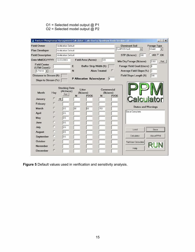
The PPM Calculator was verified for various parameters (or processes) accounted for in the model.The parameters considered were field slope, slope length, soil test P, litter and commercial P2O5application rate, litter and commercial nitrogen application rate, minimum dry forage (biomass),forage type, maximum stocking rate, hay, soil type, grazing and application timing. Most of theparameters have five different levels (values). The verification was carried out by varying oneparameter at a time from a default value, then running the model. Default values are shown inFigure 5. The levels of the variations used in the verifications are shown in Table 1. As an example,the levels of field slope factor were 0, 2, 3, 5, and 10%, with the default (median) value of 3%. Theverification results for runoff, soluble phosphorus (Sol P), organic P (Org P), sediment bound P(Sed P) and total P (TP) were as expected for our default condition (Table 1 and Appendix E).

To answer the question about the relative importance of factors that influence phosphorus loss inrunoff, the sensitivity of the PPM Calculator was tested for various parameters (or processes)accounted in the model. The parameters considered for sensitivity analysis were field slope, slopelength, soil test P, litter P2O5, commercial P2O5, litter N, commercial N, minimum dry forage(biomass), and maximum stocking rate. The tabular summary of the sensitivity analysis for all theparameters is given in Table 2, and the graphical summaries are given in Appendix E. The relativesensitivity coefficient was calculated using the following equation:

where: Sr = Relative sensitivity (non-dimensional)Pb = Parameter investigated baseline valueOb = Selected model output for baseline conditionsP1 = Parameter value adjusted less than PbP2 = Parameter value adjusted greater than Pb

15

O1 = Selected model output @ P1O2 = Selected model output @ P2

Figure 5 Default values used in verification and sensitivity analysis.

16

Table 1 Summary table for the effects of the parameters considered for verifying the PasturePhosphorus Management Calculator.

Parameters OutputRunoff (in) Soluble P

(lb/acre)Organic P(lb/acre)

Sediment P(lb/acre)

Total P(lb/acre)

Field Slope (%)0 4.06 0.91 0.00 0.00 0.912 4.05 0.91 0.01 0.02 0.943 4.05 0.91 0.01 0.03 0.955 4.05 0.91 0.03 0.06 1.0010 4.04 0.90 0.08 0.19 1.17Slope Length (ft)100 4.04 0.91 0.01 0.02 0.94200 4.05 0.91 0.01 0.03 0.95300 4.05 0.91 0.01 0.03 0.95400 4.05 0.91 0.01 0.03 0.96500 4.05 0.91 0.01 0.03 0.96STP (lb/acre)65 4.05 0.73 0.01 0.02 0.76120 4.05 0.77 0.01 0.02 0.81300 4.05 0.91 0.01 0.03 0.95500 4.05 1.06 0.01 0.04 1.111000 4.05 1.44 0.01 0.06 1.51Min Dry Forage (lb/acre)400 11.4 2.26 0.47 1.51 4.24800 4.97 1.07 0.02 0.06 1.151200 4.05 0.91 0.01 0.03 0.951600 4.02 0.91 0.01 0.03 0.952000 4.01 0.91 0.01 0.03 0.96Litter P205 (lb/acre)0 4.05 0.55 0.01 0.02 0.5760 4.05 0.91 0.01 0.03 0.95120 4.05 1.27 0.02 0.04 1.33180 4.05 1.63 0.03 0.05 1.7240 4.05 1.99 0.03 0.06 2.08Litter N (lb/acre)0 4.72 0.86 0.03 0.06 0.9560 4.05 0.91 0.01 0.03 0.95120 4.04 0.99 0.01 0.03 1.03180 4.06 1.04 0.01 0.03 1.09240 4.07 1.08 0.01 0.03 1.12Commercial N (lb/acre)0 4.30 0.87 0.02 0.05 0.9475 4.22 0.90 0.01 0.04 0.95150 4.05 0.91 0.01 0.03 0.95175 4.04 0.92 0.01 0.03 0.96200 4.03 0.93 0.01 0.03 0.97

17

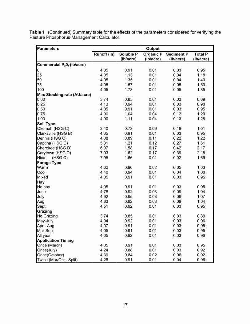
Table 1 (Continued) Summary table for the effects of the parameters considered for verifying thePasture Phosphorus Management Calculator.

Parameters OutputRunoff (in) Soluble P

(lb/acre)Organic P(lb/acre)

Sediment P(lb/acre)

Total P(lb/acre)

Commercial P205 (lb/acre)0 4.05 0.91 0.01 0.03 0.9525 4.05 1.13 0.01 0.04 1.1850 4.05 1.35 0.01 0.04 1.4075 4.05 1.57 0.01 0.05 1.63100 4.05 1.78 0.01 0.05 1.85Max Stocking rate (AU/acre)0.00 3.74 0.85 0.01 0.03 0.890.25 4.13 0.94 0.01 0.03 0.980.50 4.05 0.91 0.01 0.03 0.950.75 4.90 1.04 0.04 0.12 1.201.00 4.90 1.11 0.04 0.13 1.28Soil TypeOkemah (HSG C) 3.40 0.73 0.09 0.19 1.01Clarksville (HSG B) 4.05 0.91 0.01 0.03 0.95Dennis (HSG C) 4.08 0.89 0.11 0.22 1.22Captina (HSG C) 5.31 1.21 0.12 0.27 1.61Cherokee (HSG D) 6.97 1.58 0.17 0.42 2.17Carytown (HSG D) 7.03 1.62 0.17 0.39 2.18Nixa (HSG C) 7.95 1.66 0.01 0.02 1.69Forage TypeWarm 4.62 0.96 0.02 0.05 1.03Cool 4.40 0.94 0.01 0.04 1.00Mixed 4.05 0.91 0.01 0.03 0.95HayNo hay 4.05 0.91 0.01 0.03 0.95June 4.78 0.92 0.03 0.09 1.04July 4.92 0.95 0.03 0.09 1.07Aug 4.63 0.92 0.03 0.09 1.04Sept 4.51 0.92 0.01 0.03 0.95GrazingNo Grazing 3.74 0.85 0.01 0.03 0.89May-July 4.04 0.92 0.01 0.03 0.96Apr - Aug 4.07 0.91 0.01 0.03 0.95Mar-Sep 4.05 0.91 0.01 0.03 0.95All year 4.05 0.92 0.01 0.03 0.96Application TimingOnce (March) 4.05 0.91 0.01 0.03 0.95Once(July) 4.24 0.88 0.01 0.03 0.92Once(October) 4.39 0.84 0.02 0.06 0.92Twice (Mar/Oct - Split) 4.28 0.91 0.01 0.04 0.96

18

ParameterRunoff Soluble P Organic P Sediment P Total P

Field Slope (%) -0.001 -0.003 2.400 1.900 0.082

Slope Length (ft) 0.002 0.000 0.000 0.250 0.016

STP (lb/acre) 0.000 0.250 0.000 0.428 0.253

Min Dry Forage (lb/acre) -1.370 -1.113 -34.500 -37.000 -2.589

Litter P2O5 (lb/acre) 0.000 0.567 0.500 0.500 0.568

Litter N (lb/acre) -0.080 0.111 -1.000 -0.500 0.083

Commercial N (lb/acre) -0.050 0.049 -0.750 -0.500 0.024

Commercial P2O5 (lb/acre) 0.000 0.322 0.000 0.250 0.321

Max Stocking rate (lb/acre) 0.143 0.143 1.500 1.667 0.205

Relative Sensitivity (dimensionless)

Table 2 Summary of the sensitivity analysis of the parameters considered for the PasturePhosphorus Management Calculator.

19

PPM Calculator ValidationValidation improves the reliability of the model predictions. The validation process tests the modelwith observed data that is not used in the calibration. The PPM Calculator was not directlycalibrated; however the model makes use of SWAT parameters calibrated for the Lake EuchaBasin. The PPM Calculator was validated using 33 months of data on four fields 12 miles west ofFayetteville Arkansas. These data were presented in Edwards et al. (1994), Edwards et al. (1996a,1996b), and Edwards et al. (1997) (Appendix D). This study monitored four fields under naturalrainfall, with elevated STP due to the application of poultry litter. Two fields received additional litterduring the study period and two received only commercial nitrogen. This data-set, known as theMoore’s Creek Study, was ideal for validating the PPM Calculator.

The Moore’s Creek study contains all data required by the PPM Calculator with the exception ofminimum dry forage. Other site characteristics and management for the four fields are given inTables (3-7). Precipitation data collected at each set of fields was included in the PPM Calculatorfor the validation. Personal communication with J. F. Murdoch (2003), who was responsible for fieldwork associated with the Moore’s Creek project, stated that to the best of his recollection there werea minimum of 2-3 inches of forage and the pastures were never over grazed. Excellent conditionfertilized tall fescue contains 450-550 lbs dry forage/inch/acre (Barnhart, Stephen, ”EstimatingAvailable Forage, PM 1758”., Iowa State University Extension). We estimated minimum dry foragefor all four fields to be 500 lbs dry forage/inch/acre * 3 inches = 1500 lb dry forage/acre. We alsoelected to include a table of validation results at a minimum dry forage of 1200 lb/acre (Table 10).The results were very similar.

The overall performance of the PPM Calculator on the validation data set was excellent (Tables 8and 9). Relative errors for total and soluble P for fields RU and WU were less than 2% and -25%,respectively, and relative errors for RM and WM were higher. Relative error in predicted sedimentyields ranged from 28% to -99%. It should be noted that erosion rates from these fields are verysmall and the maximum over prediction by the model was only 69 lb/ac.

The PPM calculator performed better on fields receiving litter than those which received onlycommercial nitrogen. The PPM calculator generally under predicted total phosphorous on fieldsRM and WM, which was likely due in part to the application of poultry litter on these fields in 1991just prior to the study. Fields RM and WM experienced significant (P < 0.02) decreases in runoffsoluble phosphorous concentration during the monitoring period (Edwards et al., 1996a). Inaddition, soil test phosphorus generally decreased for these two fields during the study period(Table 6). This under prediction by the PPM Calculator for total phosphorus on these two fields isexpected because the PPM Calculator does not consider recent litter application.

20

Field Area (acre) Soil

Slope (%)

Slope Length (ft)

STP (lb/acre)

RU 3.04 Captina 3.00 450 353RM 1.41 Fayetteville 2.00 465 492WU 2.62 Allegheny-Hector-Mountainburg 4.00 590 374WM 3.61 Linker 4.00 635 727

Field Equivalent Litter

(t/acre/yr)

Commercial N (lb/acre/yr)

Ave Stocking Rate

(AU/acre/yr)RU 6 - 0.5RM - 85 0.5WU 5.5 - 0.3WM - 75 0.1

Month RU RM WU WMJan 0.7 0.7 0.3 0.1Feb 0.5 0.5 0.4 0.1Mar 0.5 0.5 0.4 0.1Apr 0.2 0.3 0.3 0.0May 0.0 0.0 0.5 0.0Jun 0.0 0.0 0.4 0.0Jul 0.0 0.0 0.4 0.0

Aug 0.5 0.5 0.3 0.2Sep 0.7 0.7 0.2 0.3Oct 0.7 0.7 0.2 0.3Nov 0.7 0.7 0.3 0.3Dec 0.7 0.7 0.3 0.3

Average 0.5 0.5 0.3 0.1

Table 3 Moore’s Creek site characteristics.

Table 4 Moore’s Creek average annual fertilizer and stocking rates.

Table 5 Moore’s Creek average monthly stocking rate for the period 8-91 to 4-94.

21

Date RU RM WU WMSTP (lb/ac) STP (lb/ac) STP (lb/ac) STP (lb/ac)

09/91 362 615 - -12/91 388 614 425 126603/92 230 420 368 78606/92 506 592 394 78709/92 493 625 416 77112/92 304 476 380 61903/93 261 395 258 60606/93 257 432 320 53709/93 397 408 357 47112/93 343 393 405 67803/94 346 441 416 753

Average 353 492 374 727

Parameter RU RM WU WM-------------------------- lb/ac/year---------------------------

NO3-N 0.24 0.38 0.25 3.01PO4-P 3.87 0.59 1.40 2.41TP 4.09 0.69 1.77 2.38NH3-N 0.36 0.18 0.88 1.13TKN 4.97 1.41 3.49 5.46COD 86.81 25.68 42.86 71.66TSS 69.19 26.31 60.75 104.59

Field Observed Runoff

(in)

Predicted Runoff

(in)

Runoff RE (%)

Observed Total P

(lb/acre)

Predicted Total P

(lb/acre)

Total P RE (%)

RU 8.2 6.7 19% 4.1 5.1 -25%RM 1.8 3.1 -76% 0.69 0.49 29%WU 2.8 3.3 -20% 1.8 2.0 -12%WM 7.4 3.5 53% 2.4 0.81 66%

Table 6 Moores Creek fields Soil Test Phosphorus (STP). Each observation is the average of fivesamples.

Table 7 Moores Creek estimated annual runoff losses of analysis parameters.

Table 8 The PPM Calculator validation results for average annual runoff volume and totalphosphorus.

22

Field Observed Soluble P (lb/acre)

Predicted Soluble P (lb/acre)

Soluble P RE (%)

Observed TSS

(lb/ac)

Predicted Sediment (lb/acre)

Sediment RE (%)

RU 3.9 3.8 2% 69 138 -99%RM 0.59 0.35 41% 26 50 -90%WU 1.4 1.6 -15% 61 44 28%WM 2.4 0.45 81% 105 90 14%

Field Observed Total P

(lb/acre)

Predicted Total P

(lb/acre)

Total P RE (%)

Observed Soluble P (lb/acre)

Predicted Soluble P (lb/acre)

Soluble P RE (%)

RU 4.1 5.3 -28% 3.9 3.9 0%RM 0.69 0.57 17% 0.59 0.36 39%WU 1.8 2.0 -12% 1.4 1.6 -15%WM 2.4 0.76 68% 2.4 0.44 82%

Table 9 PPM Calculator validation results for average soluble phosphorus and sediment.

Table 10 PPM Calculator validation using a minimum dry forage of 1200 lb/acre instead of1500/lb/acre for total and soluble phosphorus.

23

LimitationsThere are a few limitations of the PPM Calculator and SWAT models that should be noted.Limitations may be the result of data used in the model, inadequacies in the model, or using themodel to simulate situations for which it was not designed. Hydrologic models will always havelimitations, because the science behind the model is not perfect nor complete, and a model bydefinition is a simplification of the real world. Understanding the limitations helps assure thataccurate inferences are drawn from model predictions.

Because the PPM Calculator uses SWAT, it is subject to the same limitations as SWAT for pasturesystems. The selected management options are applied the same each year and do not varyingwith weather conditions for a particular year. Also, the PPM Calculator does not consider recentlitter applications, which may alter the predicted phosphorus loads in the first couple of years of thesimulation. Another limitation of the PPM calculator is the assumption of a 40 acre drainage area,which is used to predict erosion in the MUSLE equation. This assumption was required to simplifythe implementation of the PPM Calculator by the nutrient management plan developers.

The PPM Calculator predicts average monthly values based on 15 years of observed weather data.The PPM Calculator is intended to predict long term average values and is not intended to predictphosphorus load for a specific year in the future. In addition, the PPM Calculator does not currentlyconsider cultivated crops or small grains planted into pastures. One of SWAT’s strengths is itsability to examine BMPs on cultivated fields. Unfortunately, there was not time to include thiscomponent in the current version of the PPM Calculator interface.

Proposed Future WorkBelow is a list of features we will consider in release 2.0 or later versions to expand the utility of thePPM Calculator:

• Expanded simulation period with the addition of precipitation based statistical confidenceintervals on loads. This will allow the PPM Calculator to predict a probability of exceedinga particular load allocation based on weather variability.

• Account for alum treated litter. Some producers may be able to apply alum treated litterwho may not otherwise be allowed to apply untreated litter.

• Include buffer strips to allow the producer more options to meet the required phosphorusallocation.

• Activate the USLE algorithms in the SWAT model to predict erosion and eliminate the needto specify the drainage area for the field.

• Add a delivery function from field to stream to estimate the contribution of phosphorusdelivered to the stream.

• Include other Best Management Practices (BMPs) as options. The effect of some BMPscan be scientifically quantified, many others however have little research with which toconstruct a quantitative algorithm to add to the model.

24

• Evaluate the accuracy of forage yields and output the number of days grazing takes placeper month to allow the producer to use the PPM Calculator as an economic planning andmanagement tool.

25

ReferencesRedmon, L., Bidwell, T., “Stocking Rate: The key to Successful Livestock Production, F-2871”,Oklahoma Cooperative Extension Service.

Barnhart, Stephen, ”Estimating Available Forage, PM 1758”, Iowa State University Extension.

Edwards, D. R., Daniel T. C., Murdoch J. F., Vendrell P. F., Nichols D. J.. 1994. “The Moore’sCreek Monitoring Project”, Arkansas Water Resource Center Publication No. MSC-162., October21, 1994

Edwards, D. R., Daniel T. C., Murdoch J. F., Moore P. A. 1996a. “Quality of Runoff from FourNorthwest Arkansas Pasture Fields Treated with Organic and Inorganic Fertilizer”, Transactionsof the ASAE, 39(5): 1689-1696.

Edwards, D. R., Haan C.T., Sharpley A. N., Daniel T. C., Murdoch J. F., Moore P. A. 1996b.“Application of Simplified Phosphorus Transport Models to Pastures in Northwest Arkansas”,Transactions of the ASAE, 39(2): 489-496.

Edwards, D. R., Coyne M. S., Vendrell P. F., Daniel T. C., Moore P. A., Murdoch J. F. 1997. “FecalColiform and Streptococcus Concentrations in Runoff From Grazed Pastures in NorthwestArkansas”, Journal of the American Water Resources Association, 33(2):413-422. Arnold, J.G., R. Srinivasan, R. S. Mittiah, and J. R. Williams. 1998. Large Area Hydraulic Modelingand Assessment: Part I - Model Development. Journal of the American Water ResourcesAssociation, 34(1): 73-90.

Cooperative Observation Network. Surface Data Daily. NOAA. National Climatic Data Center.2003.

Haan, C.T., B.J. Barfield, J.C. Hayes. 1994. Design Hydrology and Sedimentation for SmallCatchments. Academic Press, Inc.

Lynch, S.D., Schulze, R.E. Techniques for Estimating Areal Daily Rainfallhttp://www.ccwr.ac.za/~lynch2/p241.html (2000-DEC-15).

Manure Production and Characteristics. 1995. ASAE D384.1.

Neitsch, S.L., J.G. Arnold, J.R. Williams. 2001. Soil and Water Assessment Tool User's ManualVersion 2000. Blackland Research Center.

Rollins, D. Determining Native Range Stocking Rates. OSU Extension Facts 2855.

Storm, D.E., M.J. White, M.D. Smolen. 2002. Modeling the Lake Eucha Basin Using SWAT 2000.Submitted to the Tulsa Metropolitan Utility Authority. Department of Biosystems and AgriculturalEngineering, Oklahoma State University, Stillwater, Oklahoma, August 9, 2002. (Report availableat http://biosystems.okstate.edu/home/dstorm)

Storm D. E., White M. J. “Lake Eucha Basin SWAT 2000 Model Simulations Using New RowCrop/Small Grains Soil Test Data. 2003. Submitted to the Tulsa Metropolitan Utility Authority.

26

Department of Biosystems and Agricultural Engineering, Oklahoma State University, Stillwater,Oklahoma, February 24, 2002. (Report available at http://biosystems.okstate.edu/home/dstorm)

SWAT 2000. Arnold, Jeff. et. al. USDA. Agricultural Research Service. Grassland, Soil, and WaterResearch Laboratory, 2002.

27

Appendix

Appendix A Swat Peer Reviewed Publications

Appendix B Default PPM Calculator-SWAT Input Parameters

Appendix C Relationship between Oklahoma State University and University of Arkansas SoilTest Phosphorus

Appendix D Moore’s Creek Data

Appendix E Graphical Verification Results

28

Appendix ASWAT Peer Reviewed Publications

Journal Publications and Book Chapters (as of August 21, 2003) Available online at: http://www.brc.tamus.edu/swat/swat-peerreivewed-publications.htm

Allen, P.M., J.G. Arnold, and E. Jakubowski. 1999. Prediction of stream channel erosion potential.Environmental and Engineering Geoscience V(3):339-351.

Allen, P.M., J.G. Arnold, and E. Jakubowski. 1997. Design and testing of a simple submerged jetdevice for field determination of soil erodibility. Environmental and Engineering GeoscienceIII(4):579-584.

Allen, P.M., J.G. Arnold, and W. Skipworth. 2002. Assessment of bedrock channel erosion inurban watersheds. J. of American Water Resources Association 38(5):1477-1492.

Arnold, J.G., and P.M. Allen. 1999. Automated methods for estimating baseflow and groundwaterrecharge from stream flow records. J. American Water Resources Association 35(2):411-424 .

Arnold, J.G., and P.M. Allen. 1996. Estimating hydrologic budgets for three Illinois watersheds. J.of Hydrology 176(1996):57-77.

Arnold, J.G., and Allen, P.M. 1993. A comprehensive surface-ground water flow model. J. ofHydrology 142(1993):47-69.

Arnold, J.G., P.M. Allen, and D. Morgan. 2001. Hydrologic model for design of constructedwetlands. Wetlands 21(2):167-178.

Arnold, J.G., P.M. Allen, R.S. Muttiah, and G. Bernhardt. 1995. Automated base flow separationand recession analysis techniques. Groundwater 33(6): 1010--1018.

Arnold, J.G. and R. Srinivasan. 1998. A continuous catchment-scale erosion model. In ModellingSoil Erosion by Water, NATO ASI Series, Vol. I 55: 413-427. J. Boardman and D. Favis-Mortlock,eds. Springer-Verlag Berlin Heidelberg.

Arnold, J.G., R.S. Muttiah, R. Srinivasan, and P.M. Allen. 2000. Regional estimation of base flowand groundwater recharge in the upper Mississippi basin. J. of Hydrology 227(2000):21-40.

Arnold, J. G., R. Srinivasan, and B.A. Engel. 1994. Flexible watershed configurations for simulationmodels. American Institute of Hydrology. Hydrological Science and Technology 30(1-4):5-14.

Arnold, J.G., R. Srinivasan, R.S. Muttiah, P.M. Allen and C. Walker. 1999. Continental scalesimulation of the hydrologic balance. J. American Water Resources Association 35(5):1037-1052.

Arnold, J.G., R. Srinivasan, R.S. Muttiah, and J.R. Williams. 1998. Large area hydrologic modelingand assessment part I: model development. J. American Water Resources Association 34(1):73-89.

Arnold, J.G., R. Srinivasan, T.S. Ramanarayanan, and M. Diluzio. 1999. Water resources of theTexas gulf basin. Water Science and Technology (39)3:121-133.

29

Arnold, J.G., J.R. Williams, and D.A. Maidment. 1995. A continuous time water and sedimentrouting model for large basins. J. Hydraulics Div., ASCE 121(2): 171--183.

Bingner, R.L., J. Garbrecht, J.G. Arnold, and R. Srinivasan. 1997. Effect of watershed subdivisionon simulated runoff and fine sediment yield. Transactions of the ASAE 40(5):1329-1335.

DiLuzio, M., R. Srinivasan, and J.G. Arnold. 2002. Integration of watershed tools and SWAT modelinto BASINS. J. of American Water Resources Association 38(4):1127-1141.

Eckhardt, K. and J.G. Arnold. 2001. Automatic calibration of a distributed catchment model. J. ofHydrology (251)1-2 (2001):103-109

Engel, B.A., R. Srinivasan, J.G. Arnold, C. Rewerts, and S.J. Brown. 1993. Nonpoint Source (NPS)Pollution Modeling Using Models Integrated with Geographic Information Systems (GIS). WaterScience Technology 28(3-5):685-690.

FitzHugh, T. W., and D.S. Mackay. 2000. Impacts of input parameter spatial aggregation on anagricultural nonpoint source pollution model. Journal of Hydrology 236:35-53.

Fohrer, N., K. Eckhardt, S. Haverkamp, and H.-G. Frede. 1999. Effects of land use changes on thewater balance of a rural watershed in a peripheral region. Z. f. Kulturtechnik und Landentwicklung40:1-5.

Fohrer, N., S. Haverkamp, K. Eckhardt, and H.-G. Frede. 2001. Hydrologic response to land usechanges on the catchment scale. Phys. Chem. Earth (B), 26(7-8): 577-582.

Fontaine, T.A., T.S. Cruickshank, J.G. Arnold and R.H. Hotchkiss. 2002. Development of asnowfall-snowmelt routine for mountainous terrain for the soil water assessment tool (SWAT),Journal of Hydrology 262 (1-4):209-223.

Fontaine, T.A., J.F. Klassen, T.S. Cruickshank, and R.H. Hotchkiss. 2001. Hydrological responseto climate change in the Black Hills of South Dakota, USA. Hydrological Sciences Journal46(1):27-40.

Gitau, M.W., W.J. Gburek, and A.R. Jarrett. 2002. Estimating best management practice effectson water quality in the Town Brook watershed, New York. In: Proc. Interagency Fed. ModelingMeeting Las Vegas.

Haberlandt, U., B. Klocking, V. Krysanova, and A. Becker. 2002. Regionalisation of the base flowindex from dynamically simulated flow components---a case study in the Elbe River Basin. Journalof Hydrology 248:35-53.

Haberlandt, U., V. Krysanova, B. Klocking, and A. Becker. 2001. Development of a metamodel forlarge-scale assessment of water and nutrient fluxes—first components and initial tests for the ElbeRiver basin. Proceedings of a symposium held during the Sixth IAHS Scientific Assembly atMaastricht, The Netherlands, July 2001). IAHS Publ. No. 268.

Harmel, R. D., C.W. Richardson, and K.W. King. 2000. Hydrologic response of a small watershedmodel to generated precipitation. Transactions of the ASAE 43(6):1483-1488.

30

Hotchkiss, R.H., S.F. Jorgensen, M.C. Stone, and T.A. Fontaine. 2000. Regulated river modelingfor climate change impact assessment: The Missouri River. 36(2):375-386.

King, K.W., J.G. Arnold, and R.L. Bingner. 1999. Comparison of Green-Ampt and curve numbermethods on Goodwin creek watershed using SWAT. Transactions of the ASAE 42(4):919-925.

Kirsh, K., A. Kirsh, and J.G. Arnold. 2002. Predicting sediment and phosphorus loads in the RockRiver Basin using SWAT. Transactions of the ASAE 45(6):1757-1769.

Lasch, P., M. Lindner, B. Ebert, M. Flechsig, F.-W. Grestengarbe, F. Suckow, and P.C. Werner.1999. Regional impact analysis of climate change on natural and managed forests in the FederalState of Barandenburg, Germany. Environmental Modeling and Assessment 4:273-286.

Manguerra, H.B., and B.A. Engel. 1998. Hydrologic parameterization of watersheds for runoffprediction using SWAT. J. of the American Water Resources Association 34(5):1149-1162.

Miller, S. N., W.G. Kepner, M.H. Mehaffey, M. Hernandez, R.C. Miller, D.C. Goodrich, K.KDevonald, D.T. Heggem, and W.P. Miller . 2002. Integrating landscape assessment and hydrologicmodeling for land cover change analysis. J. of American Water Resources Association38(4):915-929.

Qiu, Z., and T. Prato. 1998. Economic evaluation of riparian buffers in an agricultural watershed.J. of American Water Resources Association 34(4):877-890.

Peterson, J.R. and J.M. Hamlet. 1998. Hydrologic calibration of the SWAT model in a watershedcontaining fragipan soils. J. of American Water Resources Association 34(3): 531-544.

Ritschard, R. L., J.F. Cruise, and L.U. Hatch. 1999. Spatial and temporal analysis of agriculturalwater requirements in the Gulf Coast of the United States. J. of American Water ResourcesAssociation 35(6):1585-1596.

Rosenberg, N.J., D.L. Epstein, D. Wang, L. Vail, R. Srinivasan, and J.G. Arnold. 1999. Possibleimpacts of global warming on the hydrology of the Ogallala aquifer region. Climatic Change42(4):677-692.

Rosenthal, W.D., and D.W. Hoffman. 1999. Hydrologic modeling/GIS as an aid in locatingmonitoring sites. Transactions of the ASAE 42(6):1591-1598.

Rosenthal, W.D., R. Srinivasan, and J.G. Arnold. 1995. Alternative river management using alinked GIS-hydrology model. Transactions of the ASAE 38(3):783-790.

Saleh, A., J.G. Arnold, P.W. Gassman, L.W. Hauck, W.D. Rosenthal, J.R. Williams, and A.M.S.McFarland. 2000. Application of SWAT for the upper north Bosque watershed. Transactions of theASAE 43(5):1077-1087.

Santhi, C., J.G. Arnold, J.R. Williams, W.A. Dugas, and L. Hauck. 2001. Validation of the SWATmodel on a large river basin with point and nonpoint sources. J. of American Water ResourcesAssociation 37(5):1169-1188.

31

Santhi, C., J.G. Arnold, J.R. Williams, W.A. Dugas, and L. Hauck. 2002. Application of awatershed model to evaluate management effects on point and nonpoint source pollution.Transactions of the ASAE 44(6):1559-1570.

Sophocleous, M.A., J.K. Koelliker, R.S. Govindaraju, T. Birdie, S.R. Ramireddygari, and S.P.Perkins. 1999. Integrated numerical modeling for basin-wide water management: The case of theRattlesnake Creek basin in south-central Kansas. Journal of Hydrology 214:179-196.

Spruill, C.A., S.R. Workman, and J.L. Taraba. 2000. Simulation of daily and monthly streamdischarge from small watersheds using the SWAT model. 43(6):1431-1439.

Srinivasan, R. and J.G. Arnold. 1994. Integration of a basin-scale water quality model with GIS.Water Resources Bulletin (30)3:453-462.

Srinivasan, R.S., J.G. Arnold, and C.A. Jones. 1998. Hydrologic modeling of the United States withthe soil and water assessment tool. Water Resources Development 14(3):315-325.

Srinivasan, R., J.G. Arnold, and R.S. Muttiah. 1995. Plant and hydrologic simulation at thecontinental scale using SWAT and GIS. AIH Hydrologic Science and Technology 11(1-4):160-168.

Srinivasan, R., T.S. Ramanarayanan, J.G. Arnold, and S.T, Bednarz.. 1998. Large area hydrologicmodeling and assessment part II: model application. J. American Water Resources Association34(1):91-101.

Stone, M.C., R.H. Hotchkiss, C.M. Hubbard, T.A. Fontaine, L.O. Mearns, and J.G. Arnold. 2001.Impacts of climate change on Missouri river basin water yield. J. of American Water ResourcesAssociation 37(5):1119-1130.

Stonefelt, M. D., T.A. Fontaine, and R.H. Hotchkiss. 2000. Impacts of climate change on wateryield in the upper wind river basin. J. of American Water Resources Association 36(2):321-336.

Thomson, A.M., R.A. Brown, N.J. Rosenberg, R.C. Izaurralde, D.M. Legler, and R. Srinivasan.2003. Simulated impacts of El Nino/southern oscillation on United States water resources. J. ofAmerican Water Resources Association 39(1):137-148.

Van Griensven, A., and W. Brauwens. 2001. Integral water quality modeling of catchments. WaterScience and Technology 43(7):321-328.

Van Liew, M.W. and J. Garbrecht. 2003. Hydrologic simulation of the Little Washita Riverexperimental watershed using SWAT. J. of American Water Resources Association 39(2):413-426.

Wauchope, R.D., L.R. Ahuja, J.G. Arnold, R. Bingner, R. Lowrance, M.T. Van Genuchten, and L.D.Adams. 2002. Software for pest management science: computer models and databases for theU.S. Department of Agriculture – Agricultural Research Service. Pest Management Science59(6-7):691-698.

Weber, A., N. Fohrer and D. Moller. 2001. Long-term land use changes in a mesocale watersheddue to socio-economic factors – effects on landscape structures and functions. Ecological Modelling140:125-140.

32

Whittaker, G., R. Fare, R. Srinivasan, and D.W. Scott. 2003. Spatial evaluation of alternativenonpoint nutrient regulatory instruments. Published in Water Resources Research 39(4).

Wollmuth, J.C. and J. W. Eheart. 2000. Surface water withdrawal allocation and trading systemsfor traditionally riparian areas. J. American Water Resources Association 36(2):293-303.

33

Appendix BDefault PPM Calculator-SWAT Input Parameters

Pond Properties (.PND)Ponds were not included

In-Stream Water Quality Parameters (.SWQ)In-stream Processes are disabled.

Weather Generator (.WGN)Observed rainfall and temperature from spavianw dam weather station included.Other stats generated using default SWAT weather database for Siolam Springs.

Water Use (.WUS)No consumptive usage

Stream Channel Properties (.RTE) 10.111 | CHW2 : Main channel width [m] 2.000 | CHD : Main channel depth [m] 0.002 | CH_S2 : Main channel slope [m/m] 2.5 | CH_L2 : Main channel length [km] 0.014 | CH_N2 : Manning's nvalue for main channel 0.000 | CH_K2 : Effective hydraulic conductivity [mm/hr] 0.000 | CH_EROD: Channel erodibility factor 0.000 | CH_COV : Channel cover factor 5.000 | CH_WDR : Channel width:depth ratio [m/m] 0.000 | ALPHA_BNK : Baseflow alpha factor for bank storage [days]

Subbasin Properties (.SUB) 1 | HRUTOT : Total number of HRUs modeled in subbasin 36.343544 | LATITUDE : Latitude of subbasin [degrees] 316.69 | ELEV : Elevation of subbasin [m] 0.000 | PLAPS : Precipitation lapse rate [mm/km] 0.000 | TLAPS : Temperature lapse rate [/C/km] 0.000 | SNO_SUB : Initial snow water content [mm] 1.000 | CH_L1 : Longest tributary channel length [km] 0.002 | CH_S1 : Average slope of tributary channel [m/m] 82.111 | CH_W1 : Average width of tributary channel [mm/km] 0.500 | CH_K1 : Effective hydraulic conductivity in tributary channel[mm/hr] 0.014 | CH_N11 : Manning's "n" value for the tributary channels| HRU data files000010001.hru000010001.mgt000010001.sol000010001.chm000010001.gw

Ground Water Properties (.GW) 100.0000 | SHALLST : Initial depth of water in the shallow aquifer [mm] 1000.0000 | DEEPST : Initial depth of water in the deep aquifer [mm] 1.0000 | GW_DELAY : Groundwater delay [days] 0.1100 | ALPHA_BF : BAseflow alpha factor [days] 30.0000 | GWQMN : Threshold depth of water in the shallow aquifer requiredfor return flow to occur [mm] 0.0200 | GW_REVAP : Groundwater "revap" coefficient 10.0000 | REVAPMN: Threshold depth of water in the shallow aquifer for"revap" to occur [mm] 0.2000 | RCHRG_DP : Deep aquifer percolation fraction 1.0000 | GWHT : Initial groundwater height [m] 0.0030 | GW_SPYLD : Specific yield of the shallow aquifer [m3/m3] 0.0000 | GW_NO3 : Concentration of nitrate in groundwater contribution tostreamflow from subbasin [mg N/l] 0.0000 | GWSOLP : Concentration of soluble phosphorus in groundwatercontribution to streamflow from subbasin [mg P/l]

Basin Configuration (.BSN) 0.165 | DA_KM : Area of the watershed [km2] 0.000 | DT : . Time step for infiltration and channel routing [hr] 1.000 | SFTMP : Snowfall temperature [ºC] 0.500 | SMTMP : Snow melt base temperature [ºC] 4.500 | SMFMX : Melt factor for snow on June 21 [mm H2O/ºC-day] 4.500 | SMFMN : Melt factor for snow on December 21 [mm H2O/ºC-day] 1.000 | TIMP : Snow pack temperature lag factor

34

Appendix BDefault PPM Calculator-SWAT Input Parameters

1.000 | SNOCOVMX : Minimum snow water content that corresponds to 100%

snow cover [mm] 0.500 | SNO50COV : Fraction of snow volume represented by SNOCOVMX thatcorresponds to 50% snow cover 1.000 | RCN : Concentration of nitrogen in rainfall [mg N/l] 0.000 | SURLAG : Surface runoff lag time [days] 1.000 | APM : Peak rate adjustment factor for sediment routing in thesubbasin (tributary channels) 1.000 | PRF : Peak rate adjustment factor for sediment routing in themain channel 0.001 | SPCON : Linear parameter for calculating the maximum amount ofsediment that can be reentrained during channel sediment routing 1.500 | SPEXP : Exponent parameter for calculating sediment reentrainedin channel sediment routing 1.000 | EVRCH : Reach evaporation adjustment factor 3.000 | EVLAI : Leaf area index at which no evaporation occurs fromwater surface [m2/m2] 0.000 | FFCB : Initial soil water storage expressed as a fraction offield capacity water content 0.003 | CMN : Rate factor for humus mineralization of active organicnitrogen 20.000 | UBN : Nitrogen uptake distribution parameter 20.000 | UBP : Phosphorus uptake distribution parameter 2.000 | NPERCO : Nitrogen percolation coefficient 5.00 | PPERCO : Phosphorus percolation coefficient 300.000 | PHOSKD : Phosphorus soil partitioning coefficient 0.400 | PSP : Phosphorus sorption coefficient 0.050 | RSDCO : Residue decomposition coefficient 0.500 | PERCOP : Pesticide percolation coefficient 0 | IRTPEST : Number of pesticide to be routed through the watershedchannel network 0.000 | WDPQ : Die-off factor for persistent bacteria in soil solution.[1/day] 0.000 | WGPQ : Growth factor for persistent bacteria in soil solution[1/day] 0.000 | WDLPQ : Die-off factor for less persistent bacteria in soilsolution [1/day] 0.000 | WGLPQ : Growth factor for less persistent bacteria in soilsolution. [1/day] 0.000 | WDPS : Die-off factor for persistent bacteria adsorbed to soilparticles. [1/day] 0.000 | WGPS : Growth factor for persistent bacteria adsorbed to soilparticles. [1/day] 0.000 | WDLPS : Die-off factor for less persistent bacteria adsorbed tosoil particles. [1/day] 0.000 | WGLPS : Growth factor for less persistent bacteria adsorbed tosoil particles. [1/day] 175.000 | BACTKDQ : Bacteria partition coefficient 1.070 | THBACT : Temperature adjustment factor for bacteriadie-off/growth 0.000 | MSK_CO1 : Calibration coefficient used to control impact of thestorage time constant (Km) for normal flow 3.500 | MSK_CO2 : Calibration coefficient used to control impact of thestorage time constant (Km) for low flow 0.200 | MSK_X : Weighting factor controlling relative importance ofinflow rate and outflow rate in determining water storage in reach segment

Simulation Control File (.COD) 20 | NBYR : Number of years simulated 1970 | IYR : Beginning year of simulation 1 | IDAF : Beginning julian day of simulation 365 | IDAL : Ending julian day of simulation 0 | IPD : Print code (month, day, year) 5 | NYSKIP : Number of years to skip output printing/summarization 1 | IPRN : Print code for .std file: 0=input summary is printed 0 | ILOG : Stream flow print code: 1=print log of streamflow 1 | IPRP : Print code for .pso file: 1=print pesticide output 0 | IGN : Random number seed cycle code

35

Appendix BDefault PPM Calculator-SWAT Input Parameters

1 | PCPSIM : Precipitation simulation code: 1=measured, 2=simulated 30 | IDT : Rainfall data time step 0 | IDIST : Rainfall distribution code 0 skewed, 1 exponential 1.30 | REXP : Exponent for IDIST=1 1 | TMPSIM : Precipitation simulation code: 1=measured, 2=simulated 2 | SLRSIM : Solar radiation simulation code: 1=measured,2=simulated 2 | RHSIM : Relative humidity simulation code: 1=measured,2=simulated 2 | WINDSIM : Windspeed simulation code: 1=measured, 2=simulated 0 | IPET : PET method: 0=priest-t, 1=pen-m, 2=har, 3=read into model 0 | IEVENT : Rainfall//runoff code: 0=daily rainfall/CN 0 | ICRK : Crack flow code: 1=model crack flow in soil 0 | IRTE : Water routing method 0=variable travel time, 1 =Muskingum 0 | IDEG : Channel degradation code 0 | IRESQ : Lake water quality: 1= model lake water quality 0 | IWQ : In-stream water quality: 1= model in-stream water quality 0 | ISPROJ : special project: 1=HUMUS, 2=Missouri RiverReach output variables 0 0 0 0 0 0 0 0 0 0 0 0 0 0 0 0 0 0 0 0Subbasin output variables 0 0 0 0 0 0 0 0 0 0 0 0 0 0 0 0 0 0 0 0HRU output variables 0 0 0 0 0 0 0 0 0 0 0 0 0 0 0 0 0 0 0 0

36

Comparison of Soil Test Phosphorus Between Arkansas and Oklahoma

y = 1.05x + 8.4R2 = 0.98

n = 460

200

400

600

800

1000

0 200 400 600 800 1000Arkansas M3-P (lb/a)

Okl

ahom

a M

3-P

(lb/a

)

Appendix CRelationship between Oklahoma State Universityand University of Arkansas Soil Test Phosphorus

37

Field Date Fertilizer Type

N P

RU 03/15/92 Poultry Manure 296 10607/13/93 Poultry Manure 402 186

RM 03/23/92 NH4NO3 60 008/14/92 NH4NO3 60 004/22/93 NH4NO3 103 007/14/93 NH4NO3 121 0

WU 03/23/92 Poultry Litter 194 5508/13/92 Poultry Litter 128 5304/13/93 Poultry Litter 141 3807/20/93 Poultry Litter 173 6303/29/94 Poultry Litter 166 63

WM 03/23/92 NH4NO3 123 004/13/93 NH4NO3 91 007/20/93 NH4NO3 91 003/24/94 NH4 NO3 90 0

(lb/ac)Application Rate

Appendix DMoores Creek Data

Table D1 Manure and commercial fertilizer application by field.

38

Month FieldRU RM WU WM

08/91 2.0 2.0 0.3 0.309/91 2.0 2.0 0.3 0.310/91 2.0 2.0 0.3 0.311/91 2.0 2.0 0.3 0.312/91 2.0 2.0 0.3 0.301/92 2.0 2.0 0.3 0.302/92 2.0 2.0 1.0 0.003/92 2.0 2.0 1.0 0.004/92 0.0 0.0 1.0 0.005/92 0.0 0.0 1.0 0.006/92 0.0 0.0 1.0 0.007/92 0.0 0.0 1.7 0.008/92 0.0 0.0 1.7 0.009/92 1.5 1.5 1.1 1.110/92 1.5 1.5 1.1 1.111/92 1.5 1.5 1.1 1.112/92 1.5 1.5 1.1 1.101/93 1.5 1.5 1.5 0.002/93 1.5 1.5 1.5 0.003/93 1.5 1.5 1.5 0.004/93 1.5 1.5 1.5 0.005/93 0.0 0.0 1.5 0.006/93 0.0 0.0 0.9 0.007/93 0.0 0.0 0.0 0.008/93 1.4 1.4 0.0 1.009/93 1.4 1.4 0.0 1.010/93 1.4 1.4 0.0 1.011/93 1.4 1.4 0.5 0.512/93 1.4 1.4 0.5 0.501/94 1.4 1.4 0.5 0.502/94 0.0 0.0 0.5 0.503/94 0.0 0.0 0.5 0.504/94 0.0 1.0 0.0 0.0

-----------animal units/ha----------------

Appendix DMoores Creek Data

Table D2 Stocking rate by field.

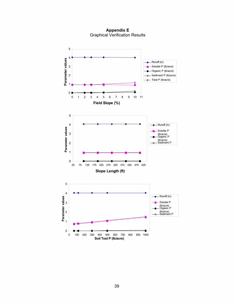
39

0

1

2

3

4

5

0 1 2 3 4 5 6 7 8 9 10 11

Field Slope (%)

Para

met

er v

alue

sRunoff (in)Soluble P (lb/acre)Organic P (lb/acre)Sediment P (lb/acre)Total P (lb/acre)

0

1

2

3

4

5

25 75 125 175 225 275 325 375 425 475 525

Slope Length (ft)

Para

met

er v

alue

s

Runoff (in)

Soluble P(lb/acre)Organic P(lb/acre)Sediment P

0

1

2

3

4

5

0 100 200 300 400 500 600 700 800 900 1000Soil Test P (lb/acre)

Para

met

er v

alue

s Runoff (in)

Soluble P(lb/acre)Organic P(lb/acre)Sediment P

Appendix EGraphical Verification Results

40

0

2

4

6

8

10

12

0 300 600 900 1200 1500 1800 2100Minimum Dry Forage (lb/acre)

Para

met

er v

alue

s Runoff (in)

Soluble P(lb/acre)Organic P(lb/acre)Sediment P

0

1

2

3

4

5

0 50 100 150 200 250Litter P2O5 (lb/acre)

Para

met

er v

alue

s

Runoff (in)

Soluble P(lb/acre)Organic P(lb/acre)Sediment P

0

1

2

3

4

5

0 50 100 150 200 250

Litter N (lb/acre)

Para

met

er v

alue

s

Runoff (in)

Soluble P(lb/acre)Organic P(lb/acre)Sediment P

Appendix E Graphical Verification Results (Continued)

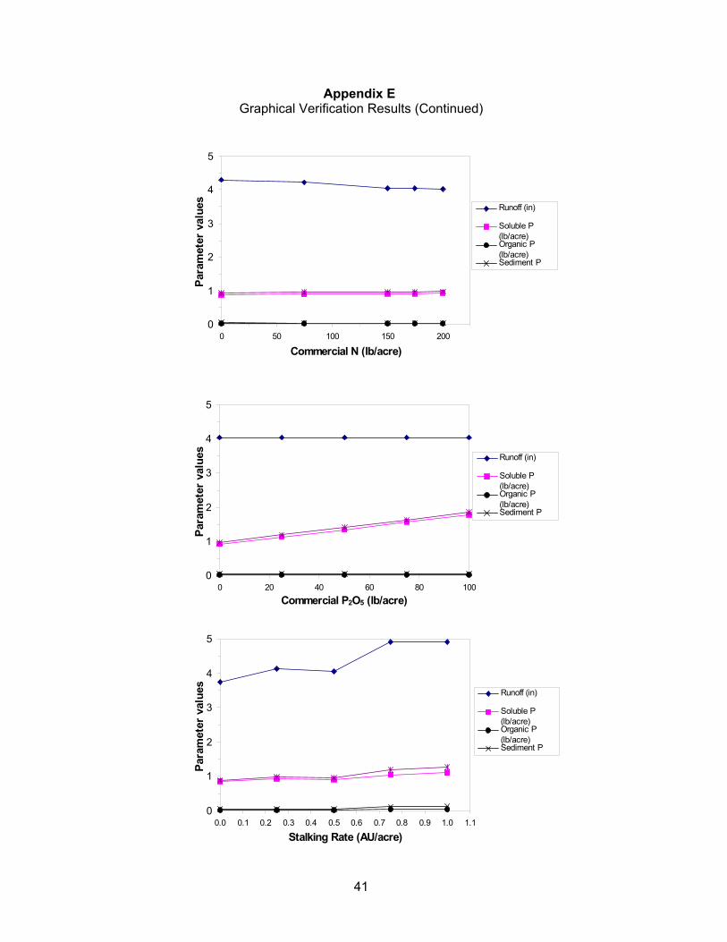
41

0

1

2

3

4

5

0 50 100 150 200

Commercial N (lb/acre)

Para

met

er v

alue

sRunoff (in)

Soluble P(lb/acre)Organic P(lb/acre)Sediment P

0

1

2

3

4

5

0 20 40 60 80 100Commercial P2O5 (lb/acre)

Para

met

er v

alue

s

Runoff (in)

Soluble P(lb/acre)Organic P(lb/acre)Sediment P

0

1

2

3

4

5

0.0 0.1 0.2 0.3 0.4 0.5 0.6 0.7 0.8 0.9 1.0 1.1

Stalking Rate (AU/acre)

Para

met

er v

alue

s

Runoff (in)

Soluble P(lb/acre)Organic P(lb/acre)Sediment P

Appendix E Graphical Verification Results (Continued)

42

0

1

2

3

4

5

6

7

8

Okemah(HSG C)

Clarksville(HSG B)

Dennis(HSG C)

Captina(HSG C)

Cherokee(HSG D)

Carytown(HSG D)

Nixa (HSG C)

Soil Type

Para

met

er v

alue

sRunoff (in)

Soluble P(lb/acre)Organic P(lb/acre)Sediment P

0

1

2

3

4

5

Warm Cool Mixed

Forage Type

Para

met

er v

alue

s Runoff (in)

Soluble P(lb/acre)Organic P(lb/acre)Sediment P

0

1

2

3

4

5

No hay June July Aug Sept

Hay

Para

met

er v

alue

s

Runoff (in)

Soluble P(lb/acre)Organic P(lb/acre)Sediment P

Appendix E Graphical Verification Results (Continued)

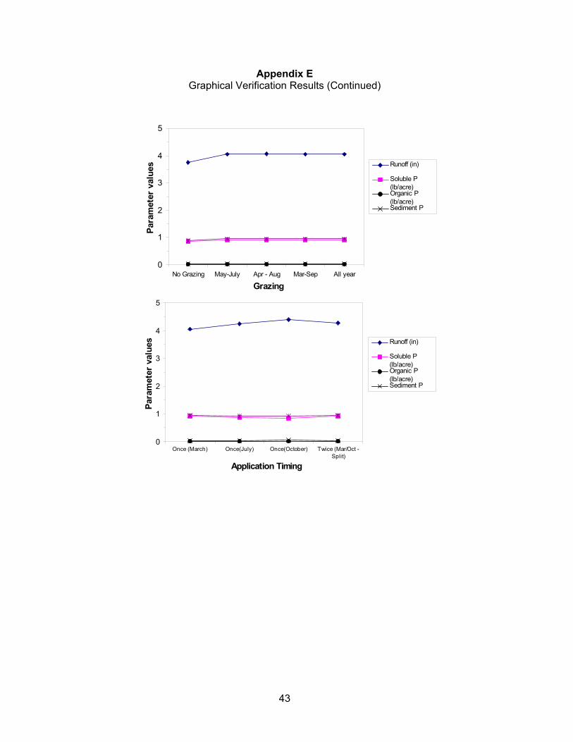
43

0

1

2

3

4

5

No Grazing May-July Apr - Aug Mar-Sep All year

Grazing

Para

met

er v

alue

s Runoff (in)

Soluble P(lb/acre)Organic P(lb/acre)Sediment P

0

1

2

3

4

5

Once (March) Once(July) Once(October) Twice (Mar/Oct -Split)

Application Timing

Para

met

er v

alue

s Runoff (in)

Soluble P(lb/acre)Organic P(lb/acre)Sediment P

Appendix EGraphical Verification Results (Continued)