past week - miramareperessi/non-uniform.pdf · 3. intrinsic generators consider the subroutine that...

3. Intrinsic generators

Consider the subroutine that generates random numbers: e.g., in For-tran 90 random number() is an intrinsic procedure generating real randomnumbers in the range [0,1[. The argument of the subroutine random number()is real, has intent out, and can be a scalar or an array.See for instance rantest intrinsic.f90 (don’t worry about the seed ofthe sequence). Note in the example the use of the dynamical allocationof memory (the instruction allocatable) for the array x and the use ofprint instruction with a specified format.

(a) Produce a sequence (long enough) of random numbers in [0,1[ withthe intrinsic generator of your favorite compiler. Test uniformity andcorrelation (see points b) e c) of Ex. 2) on this sequence. What doyou see? Any di↵erence with respect to Ex. 2?

(b) (optional) For a quantitative test of uniformity consider the momentof order k:

hxki = 1

N

NX

i=1

x

ki =

Z 1

0dx x

kP (x) + O(1/

pN).

For the uniform distribution pu(x) in [0,1[, i.e. for

pu(x) =n1 for 0 x 10 outside

we have hxki = 1/(k + 1). Consider the sequence

��1

N

NX

i=1

x

ki � 1

k + 1

��

and study the asymptotic behaviour for large N . If the behaviour is⇠ 1/

pN , then the distribution is random and uniform. Do the test

for k=1, 3, 7, and N=100, 10.000, 100.000.

(c) (optional) A quantitative test for correlation is to calculate

C(k) =1

N

NX

i=1

xixi+k ⇡Z 1

0dx

Z 1

0dy xy P (x, y).

For the uniform distribution pu(x) with x and y totally uncorrelated,we have C(k) = 1/4. If our random number distribution is uniformenough and with small correlation, we expect C(k) � 1/4 ⇠ 1/

pN .

What can you tell about the sequence above?

3


Consider the subroutine that generates random numbers: e.g., in For-tran 90 random number() is an intrinsic procedure generating real randomnumbers in the range [0,1[. The argument of the subroutine random number()is real, has intent out, and can be a scalar or an array.See for instance rantest intrinsic.f90 (in this exercise don’t worryabout the seed of the sequence). Note in the example the use of the dyna-mical allocation of memory (the instruction allocatable) for the array xand the use of print instruction with a specified format.


(b) For a quantitative test of uniformity consider the moment of order k:

hxkicalc = 1

N

NX

i=1

x

ki ; hxkith =

Z 1

0dx x

kP (x)



we have hxkith = 1/(k + 1). Consider the error

�N (k) =��hxkicalc � hxkith

�� =

��1

N

NX

i=1

x

ki � 1

k + 1

��

for the expected moment of order k and study its asymptotic beha-viour for large N . If the behaviour is ⇠ 1/

pN , then the distribution

is random and uniform. Do the test for k=1, 3, 7, and N=100,10.000, 100.000.

(c) A quantitative test for correlation is to calculate

C(k)calc =1

N

NX

i=1

xixi+k; C(k)th =

Z 1

0dx

Z 1

0dy xy P (x, y).

For the uniform distribution pu(x) with x and y totally uncorrelated,we have C(k)th = 1/4. If our random number distribution is uni-form enough and with small correlation, we expect

��C(k)calc � 1/4

�� ⇠1/pN . What can you tell about the sequence above?

3

past week:





hxki = 1

N

NX

i=1

x

ki =

Z 1

0dx x

kP (x) + O(1/

pN).




��1

N

NX

i=1

x

ki � 1

k + 1

��



for k=1, 3, 7, and N=100, 10.000, 100.000.


C(k) =1

N

NX

i=1

xixi+k ⇡Z 1

0dx

Z 1

0dy xy P (x, y).


pN .


3





hxki = 1

N

NX

i=1

x

ki =

Z 1

0dx x

kP (x) + O(1/

pN).




��1

N

NX

i=1

x

ki � 1

k + 1

��



for k=1, 3, 7, and N=100, 10.000, 100.000.


C(k) =1

N

NX

i=1

xixi+k ⇡Z 1

0dx

Z 1

0dy xy P (x, y).


pN .


3

numerically calculated

from the sequence

expected if the sequence

were truly uniform

deviation of <x>k =

log(deviation of <x>k) ~ -1/2 log(N) + cost.’

+ cost.

check the slope of the log-log !!!

do you want to check a power law?

linear regression: much better

very small deviations from the expected behavior could be accidental;

check the overall behavior, and try also changing the seed!

k=1k=3k=7

the higher is the order of the momentum, the more meaningful is the test(two functions may have the same average (<x>) although they are very different!):

check the behavior for higher-order momenta!

Random numbers with non uniform

distributionsand random processes

M. Peressi - UniTS - Laurea Magistrale in PhysicsLaboratory of Computational Physics - Unit III

last lecture:

generation of real (pseudo)random numberswith uniform distribution in [0;1[

@⇢

@t

= r

pu(x) =

n1 0 x < 1

0 otherwise

1

@⇢

@t

= r

pu(x) =

n1 0 x < 1

0 otherwise

1

@⇢

@t

= r

pu(x) =

n1 0 x < 1

0 otherwise

1

Part I - Random numbers with non uniform distributions:

How can we generate random numbers with a given distribution p(x) ?

@⇢

@t

= r

pu(x) =

n1 0 x < 1

0 otherwise

p(x)

1

@⇢

@t

= r

pu(x) =

n1 0 x < 1

0 otherwise

1

Part I - Random numbers with non uniform distributions:

1) inverse transformation method (general)2) rejection method (general)3) some “ad hoc” methods: the Box-Muller algorithm for the gaussian distribution

@⇢

@t

= r

pu(x) =

n1 0 x < 1

0 otherwise

p(x)

1

@⇢

@t

= r

pu(x) =

n1 0 x < 1

0 otherwise

1

Non uniform random numbers distribution:1) inverse transformation method (general)

Inverse transform method 3 – 2

Generating random numbers

Problem: Generate sample of a random variable X with a givendensity f . (The sample is called a random variate)

What does this mean ?

Answer: Develop an algorithm such that if one used it repeatedly(and independently) to generate a sequence of samplesX1, X2, . . . , Xn then as n becomes large, the proportion of samplesthat fall in any interval [a, b] is close to P(X ! [a, b]), i.e.

#{Xi ! [a, b]}n

" P(X ! [a, b])

Solution: 2-step process

• Generate a random variate uniformly distributed in [0, 1] .. alsocalled a random number

• Use an appropriate transformation to convert the random numberto a random variate of the correct distribution

why is this approach good ?

Answer: Focus on generating samples from ONE distribution only.

Problem: Generate sample of a random variable (or variate) x with a given distribution p .

Non uniform random numbers distribution:1) inverse transformation method - algorithm

3.2.2 Transformation Method http://homepage.univie.ac.at/Franz.Vesely/cp0102/dx/node40.html

1 of 1 18-10-2005 0:14

Next: 3.2.3 Generalized Transformation Method: Up: 3.2 Other Distributions Previous: 3.2.1 Transformation of probability

3.2.2 Transformation Method

Given a probability density :

Find a bijective mapping such that the distribution of is :

$\displaystyle p(x)$

It is easy to see that

fulfills this condition, with .

EXAMPLE: Let


Then , with the inverse . Therefore:

Sample equidistributed in .

Compute .

Geometrical interpretation:

is sampled from an equidistribution and .

The regions where is steeper (i.e. is large) are hit more frequently.

Franz J. Vesely Oct 2005See also: "Computational Physics - An Introduction," Kluwer-Plenum 2001

! +!

"!

p(x)dx = 1

y = P (x) =! dy = dP (x) =! pu(y)dy = dP (x) (since pu(y) = 1 for 0 " y " 1)

cumulative distribution function P(x)

But : dP (x) = p(x)dx, therefore p(x)dx = pu(y)dy

@⇢

@t

= r

p

u

(x) =

n1 0 x < 1

0 otherwise

Let p(x) be a desired distribution, and y = P (x) =

Zx

�1p(x

0)dx

0the corresponding cumulative distribution.

Assume that P

�1(y) is known.

• Sample y from an equidistribution in the interval (0,1). (i.e., use p

u

(y))

• Compute x = P

�1(y).

The variable x then has the desired probability density p(x).

1

3.2.2 Transformation Method http://homepage.univie.ac.at/Franz.Vesely/cp0102/dx/node40.html

1 of 1 18-10-2005 0:14

Next: 3.2.3 Generalized Transformation Method: Up: 3.2 Other Distributions Previous: 3.2.1 Transformation of probability

3.2.2 Transformation Method

Given a probability density :

Find a bijective mapping such that the distribution of is :


It is easy to see that

fulfills this condition, with .

EXAMPLE: Let


Then , with the inverse . Therefore:

Sample equidistributed in .

Compute .

Geometrical interpretation:

is sampled from an equidistribution and .

The regions where is steeper (i.e. is large) are hit more frequently.

Franz J. Vesely Oct 2005See also: "Computational Physics - An Introduction," Kluwer-Plenum 2001

Non uniform random numbers distribution:1) inverse transformation method - the concept

intuitive rationale: also a regular uniform sampling in ygives a sampling in x with density proportional to p(x)

cumulative distribution function P(x)

Non uniform random numbers distribution:1) inverse transformation method - examples

1)

2)

p(x) =

!

1

b!aa ! x ! b

0 otherwise

P (x) =

!

0 x ! a" x

a

1

b!adx" = x!a

b!aa ! x ! b

1 x > b

P (x) =! 0 x ! 0

1 " e!ax x # 0

p(x) =! 0 x ! 0

ae!ax

x " 0

y =

y =

x = !

1

aln(1 ! y) or (same distribution!) x = !

1

aln y

x = y(b ! a) + a

Non uniform random numbers distribution:2) rejection method (general)

Due to Von Newmann (1947). Applicable to almost all distributions.Can be inefficient if the area of the rectangle is large comparedto the area below the curve p(x)

3.2.4 Rejection Method http://homepage.univie.ac.at/Franz.Vesely/cp0102/dx/node42.html

1 of 2 18-10-2005 0:38

Next: 3.2.5 Multivariate Gaussian Distribution Up: 3.2 Other Distributions Previous: 3.2.3 Generalized Transformation Method:

3.2.4 Rejection Method

A classic: created by John von Neumann, applicable to almost any .

Here is the original formulation:

And this is how we read it today:

The method is simple and fast, but it becomes inefficient whenever the area of the rectangle is large compared to the area below the graph of

. Otherwise, the ``Improved Rejection Method'' may be applicable:

@⇢

@t

= r

pu(x) =

n1 0 x < 1

0 otherwise

Let [a, b] be the allowed range of values of the variate x, and pm the maximum of the distribution p(x).

1. Sample a pair of equidistributed random numbers, x 2 [a, b] and y 2 [0, pm].

2. If y p(x), accept x as the next random number, otherwise return to step 1.

The variable x then has the desired probability density p(x).

1

p(x)accept

reject

pm

a bx

(x,y)

(x,y)

Non uniform random numbers distribution:3) gaussian distribution

@⇢

@t

= r

pu(x) =

n1 0 x < 1

0 otherwise

p(x)

1

@⇢

@t

= r

pu(x) =

n1 0 x < 1

0 otherwise

1

How to produce numbers with gaussian distribution?

- Inverse transformation method: impossibleThe cumulative distribution function P(x) cannot be analytically calculated!

- Rejection method: inefficient

p(x) =1

!

1!

2"e!x2/(2!2)

Non uniform random numbers distribution:3) gaussian distribution - Box-Muller technique

p(x) =1

!

1!

2"e!x2/(2!2)

Hint: consider the distribution in 2D instead of 1D (here σ =1 ):

p(x)p(y)dxdy = (2!)!1 e!(x2+y2)/2 dxdy



r =

!

x2 + y2 ! = arctan (y/x) ! ! r2/2Use polar coordinates: , ; def.:

(x,y)

θr

p(x) =1

!

1!

2"e!x2/(2!2)




r =

!

x2 + y2 ! = arctan (y/x) ! ! r2/2

p(x)p(y) dx dy = p(!, ") d! d" = (2#)!1 e!! d! d"

Use polar coordinates: , ; def.:dxdy = r dr d! = d" d!

and therefore:

p(x) =1

!

1!

2"e!x2/(2!2)




r =

!

x2 + y2 ! = arctan (y/x) ! ! r2/2

p(x)p(y) dx dy = p(!, ") d! d" = (2#)!1 e!! d! d"

Use polar coordinates: , ; def.:

If !

! exponentially distributed" uniformly distributed in[0, 2#]

!

"

#

"

$

x = r cos ! =!

2" cos !y = r sin ! =

!2" sin !

x, y have gaussian distributionwith "x# = "y# = 0 and # = 1

dxdy = r dr d! = d" d!and therefore:


p(x) =1

!

1!

2"e!x2/(2!2)

Non uniform random numbers distribution:3) gaussian distribution - Box-Muller recipe #1

X, Y ! [0, 1["

!

! = # ln(X) distributed with p(!) = e!!

" = 2#Y distributed with (2#)!1pu

!

x = r cos ! =!

"2 lnX cos(2"Y )y = r sin ! =

!

"2 lnX sin(2"Y )

Recipe #1 (BASIC FORM):

If !


!

"

#

"

$

x = r cos ! =!

2" cos !y = r sin ! =

!2" sin !


X, Y unif. distrib. in [0, 1[

{

NOTE:x, y are normally distributed and statistically independent. Gaussian variates with given variances σx, σy are obtained by multiplying x and y by σx and σy respectively

Non uniform random numbers distribution:3) gaussian distribution - Box-Muller recipe #2

Recipe #2 (POLAR FORM) (implemented in boxmuller.f90) :

If !


!

"

#

"

$

x = r cos ! =!

2" cos !y = r sin ! =

!2" sin !


XY R .

Advantages: avoids the calculations of sin and cos functions

@⇢

@t= r

8><

>:

X, Y uniformly distributed in [�1,1];

take (X,Y ) only within the unitary circle;

) R2= X2

+ Y 2is

uniformly distributed in [0,1]

1

@⇢

@t

= r8><

>:



) R

2= X

2+ Y

2is


8>>>>>><

>>>>>>:

x =

p�2 lnR

2X

R

y =

p�2 lnR

2Y

R

since:

cos ✓ =

X

R

, sin ✓ =

Y

R

1

on $/home/peressi/comp-phys/III-random-non-uniform-and-processes/f90 [do: $cp /home/peressi/... .../f90/* .]

expdev.f90 boxmuller.f90

Some programs:

subroutine expdev(x) REAL, intent (out) :: x REAL :: r do call random_number(r) if(r > 0) exit end do x = -log(r) END subroutine expdev

r is generated in [0,1[ ;but r=0 has to be discarded;if r=0, generate another random number;if not, exit from the unbounded loop and calculate its log

A look at the expdev.f90 code

SUBROUTINE gasdev(rnd) IMPLICIT NONE REAL, INTENT(OUT) :: rnd REAL :: r2, x, y REAL, SAVE :: g LOGICAL, SAVE :: gaus_stored=.false. if (gaus_stored) then rnd=g gaus_stored=.false. else do call random_number(x) call random_number(y) x=2.*x-1. y=2.*y-1. r2=x**2+y**2 if (r2 > 0. .and. r2 < 1.) exit end do r2=sqrt(-2.*log(r2)/r2) rnd=x*r2 g=y*r2 gaus_stored=.true. end ifEND SUBROUTINE gasdev

Every two callsuses the random number already generated in the previous call

A look at the boxmuller.f90 code

@⇢

@t

= r8><

>:



) R

2= X

2+ Y

2is


x =

p�2 lnR

2X

R

= X

p�2 lnR

2/R

2

1

since:(thus avoiding the calculation of

another √ to calculate R separately)

#include <math.h>

float gasdev(long *idum){ float ran1(long *idum); static int iset=0; static double gset; double fac,rsq,v1,v2;

if (iset == 0) { do { v1=2.0*ran1(idum)-1.0; v2=2.0*ran1(idum)-1.0; rsq=v1*v1+v2*v2; } while (rsq >= 1.0 || rsq == 0.0); fac=sqrt(-2.0*log(rsq)/rsq); gset=v1*fac; iset=1; return (float)(v2*fac); } else { iset=0; return (float)gset; }}

Every two callsuses the random number already generated in the previous call

A look at the gasdev.c code

@⇢

@t

= r8><

>:



) R

2= X

2+ Y

2is


x =

p�2 lnR

2X

R

= X

p�2 lnR

2/R

2

1

since:(thus avoiding the calculation of another √ to calculate R separately)

(optional, but useful!)

random.f90 (is a module)t_random.f90

to compile: $gfortran random.f90 t_random.f90(the module first!)

Other programs:

in the same directories indicated before:

Part II - Using random numbers

to simulate random processes

Random processes: radioactive decay

Atoms present at time Probability for each atom to decay inAtoms which decay between and

t

!N(t)

!N(t) = !!N(t)!t

N(t) = N(t = 0)e!!t

t + !t

N(t)

t

we use the probability of decay of each atomto simulate the behavior of the number of atoms left;we should be able to obtain (on average):

!

!

!t

DO ! loop on time DO i = 1, nleft ! loop on all the nuclei left call random_number(r) IF (r <= lambda) THEN ! BASIC ALGORITHM nleft = nleft -1 ! update the nuclei left (*) ENDIF END DO WRITE (unit=7,fmt=*) t , nleft if (nleft == 0) exit t = t + 1 END DO

Radioactive decay:numerical simulation

A scheme for the

simulation

1. Assign a value to the decay constant � 1 (the

probability for each nucleus to decay in a given

interval of time �t)

� establishes the time scale; one iteration in the “do loop”

corresponds to one time step �t

2. Start with Nleft = Nstart= total number of

nuclei at time t = 0

3. Basic algorithm: for each nucleus left (not yet

decayed):

• Generates a random number 0 x 1

• if x �, the nucleus decays and Nleft =

Nleft - 1, otherwise it remains and Nleft is

unchanged.

4. Repeat for each nucleus

5. Repeat the cycle for the next time step

A scheme for the

simulation

1. Assign a value to the decay constant � 1 (the

probability for each nucleus to decay in a given

interval of time �t)

� establishes the time scale; one iteration in the “do loop”

corresponds to one time step �t

2. Start with Nleft = Nstart= total number of

nuclei at time t = 0

3. Basic algorithm: for each nucleus left (not yet

decayed):

• Generates a random number 0 x 1

• if x �, the nucleus decays and Nleft =

Nleft - 1, otherwise it remains and Nleft is

unchanged.

4. Repeat for each nucleus

5. Repeat the cycle for the next time step

Note: “exit” ≠ “cycle”

Note: unbounded loop

(*) Notice that the upper bound of the inner loop (nleft) is changed within the execution of the loop; but with most compilers, in the execution the loop goes on up to the initial value of nleft; this ensures that the implementation of the algorithm is correct. The program checkloop.f90 is a test for the behavior of the loop. Look also at decay_checkloop.f90. If nleft would be changed (decreased) during the execution, the effect would be an overestimate of the decay rate. CHECK with your compiler!

decay.f90 decay_checkloop.f90

checkloop.f90

Programs:

in the same directory indicated before:

[name:] DO exit [name]

or [name:] DO END DO [name]

(name is useful in case of nested loops for explicitly indicating from which loop to exit)

possible forms of "do while": DO if (condition)exit END DOor: DO WHILE (.not. condition) ... END DO NOTE: first is better (“if () ..exit” can be placed everywhere in the loop, whereas DO WHILE must execute the loop up to the end)

- Other note:Difference between EXIT and CYCLE

Details on Fortran: unbounded loops

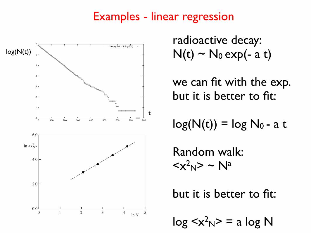
plot of the results of decay simulation (N vs t)with N=1000

N(t) ~ N0 exp(- a t)

semilog plot (log(N) vs t)=> log(N(t)) = log N0 - a t=> slope is -a

Radioactive decay:results of numerical simulation

0

200

400

600

800

1000

0 100 200 300 400 500 600 700 800

’decay.dat’

0

1

2

3

4

5

6

7

0 100 200 300 400 500 600 700 800

’decay.dat’ u 1:(log($2))

log(N(t))

N(t)

t

t

Semilog plot of the results of decay simulation for the same decay rate and different initial number of atoms:almost a straight line, but withimportant deviations (stochastic) for small N

Radioactive decay:results of numerical simulation

Page P002.html http://www.physics.orst.edu/~rubin/CPbook/chap7/P002.html

1 of 1 17-10-2005 15:54

: Slide 2 of 16.

Click slide for next, or go to previous, first, or last slide, or back to thumbnail layout.

Click slide for next, or goto previous, or back to thumbnail layout.

numerical simulations: OK on average and for large numbers

Other random processes: order and disorder

A box is divided into two parts communicating through a small hole. One particle randomly can pass through the hole per unit time, from the left to the right or viceversa.

Nleft(t): number of particles present at time t in the left sideGiven Nleft(0), what is Nleft(t) ? (see later, lectures on the statistical ensembles)

Random Walk Simulation http://www.krellinst.org/UCES/archive/modules/monte/node4.html

1 of 1 24-10-2005 10:45

Next: ProjectUp: MONTE-CARLO TECHNIQUESPrevious: Project

Random Walk Simulation

Random walk of 1000 steps going nowhere

Many physical processes such as Brownian motion, electron transport through metals, and round offerrors on computers are modeled as a random walk. In this model, many steps are taken with thedirection of each step independent of the direction of the previous one. For our model, we start at theorigin and take steps of lengths (not coordinates) in the x and y directions of

where there are a total of N steps. The distance from the starting point R is related to these steps by

Now while (2) is quite general for any walk you may take, if it is a random walk then you are equallylikely to move forwards as backwards in each step - as well as to the right or left. So on the average, for a large number of steps, all the cross terms in (2) will vanish and we are left with

where is the square root of the average squared step size or root mean squared step size. Note, thesame result obtains for a three dimensional walk. According to (3), even though the total distance

walked is , on the average, the distance from the starting point is only .

Here are different methods to generate 2-D unit steps.

Project

Next: ProjectUp: MONTE-CARLO TECHNIQUESPrevious: Project

(see next lecture)

Other random processes: random walks

Part III - Fitting data

Least-square method

• Suppose to have ND data (independent measure-ments of the variable y which is function of thevariable x):

(xi, yi ± �i), i = 1, ND

with ±�i error associated to the i value of y.

• Purpose: determine the function y = f(x) whichbetter described these data. If the analytic form ofthe function is known, a part from a set MP of pa-rameters {a1, a2 . . . , aMP

}, i.e., f(x) = f(x; {am}),the goal is to find the best set of parameters.

• To test whether the data fit via f(x) is good ornot calculate the quantity

⇥2 :=NDX

i=1

yi � f(xi; {am})

�i

!2

Note that by dividing by �i, data with larger errorshave smaller weight in this weighted average.

• The smallest ⇥2, the better the fit is.

• Least-squares fitting: The parameters MP thatminimize ⇥2 are found by:

⌅⇥2

⌅am= 0 (m = 1, MP )

=⇤ND�

i=1

yi � f(xi)

�2i

⌅f(x; {am})⌅am

= 0 (1)

• If f(x; a, b) = ax+b (linear regression), the equa-tions giving ⇥2 minimum reduce to:

a =SSxy � SxSy

�, b =

SxxSy � SxSxy

�

S =ND�

i=1

1

�2i

, Sx =ND�

i=1

xi

�2i

Sy =ND�

i=1

yi

�2i

, Sxx =ND�

i=1

x2i

�2i

Sxy =ND�

i=1

xiyi

�2i

, � = SSxx � S2x (2)

example: see program fit.f90

• Least-squares fitting: The parameters MP thatminimize ⇥2 are found by:

⌅⇥2

⌅am= 0 (m = 1, MP )

=⇤ND�

i=1

yi � f(xi)

�2i

⌅f(x; {am})⌅am

= 0 (1)

• If f(x; a, b) = ax+b (linear regression), the equa-tions giving ⇥2 minimum reduce to:

a =SSxy � SxSy

�, b =

SxxSy � SxSxy

�

S =ND�

i=1

1

�2i

, Sx =ND�

i=1

xi

�2i

Sy =ND�

i=1

yi

�2i

, Sxx =ND�

i=1

x2i

�2i

Sxy =ND�

i=1

xiyi

�2i

, � = SSxx � S2x (2)

0

1

2

3

4

5

6

7

0 100 200 300 400 500 600 700 800

’decay.dat’ u 1:(log($2))

log(N(t))

t

radioactive decay:N(t) ~ N0 exp(- a t)

we can fit with the exp.but it is better to fit:

log(N(t)) = log N0 - a t

Examples - linear regression

Random walk:<x2N> ~ Na

but it is better to fit:

log <x2N> = a log N

CHAPTER 7. RANDOM PROCESSES 231

0.0

2.0

4.0

6.0

0 1 2 3 4 5ln N

ln <x2

N>

Figure 7.2: Plot of ln!x2N " versus ln N for the data listed in Table 7.2. The straight line y =

1.02x + 0.83 through the points is found by minimizing the sum (7.19).

is that the most probable error in m and b, !m and !b respectively, is given by

!m =1#n

!y

!x(7.27a)

!b =1#n

!x2

"1/2

!x!y, (7.27b)

where

!2y =

1n $ 2

n#

i=1

d2i , (7.27c)

and di is given by (7.18). Because there are n data points, we might have guessed that n ratherthan n $ 2 would be present in the denominator of (7.27c). The reason for the factor of n $ 2 isrelated to the fact that to determine !y, we first need to calculate two quantities m and b, leavingonly n $ 2 independent degrees of freedom. To see that the n $ 2 factor is reasonable, considerthe special case of n = 2. In this case we can find a line that passes exactly through the two datapoints, but we cannot deduce anything about the reliability of the set of measurements becausethe fit always is exact. If we use (7.27c), we see that both the numerator and denominator wouldbe zero, and hence !y = 0/0, that is, !y is undetermined. If a factor of n appeared in (7.27c)instead, we would conclude that !y = 0/2 = 0, an absurd conclusion. Usually n >> 1, and thedi"erence between n and n $ 2 is negligible.

For our example, !y = 0.03, !b = 0.07, and !m = 0.02. The uncertainties "m and "# arerelated by 2"# = "m. Because we can associate "m with !m, we conclude that our best estimate

Suppose you want to fit your data (say, ‘data.dat’) with an exponential function.You have to give: 1) the functional form ; 2) the name of the parameters

gnuplot> f(x) = a * exp (-x*b)

Then we have to recall these informations together with the data we want to fit:it can be convenient to inizialize the parameters:gnuplot> a=0. ; b=1. (for example)

gnuplot> fit f(x) 'data.dat' via a,b

On the screen you will have something like:

Final set of parameters Asymptotic Standard Error ======================= ==========================

a = 1 +/- 8.276e-08 (8.276e-06%) b = 10 +/- 1.23e-06 (1.23e-05%)

correlation matrix of the fit parameters:

a b a 1.000 b 0.671 1.000

It’s convenient to plot together the original data and the fit:

gnuplot> plot f(x), 'data.dat'

Example: fit using gnuplot - I

If you prefer to use linear regression, use logarithmic data in the data file, or directlyfit the log of the original data using gnuplot:

gnuplot> f(x) = a + b*x

Then we have to recall these informations together with the data we want to fit(in the following example: x=log of the first column; y=log of the second column): gnuplot> fit f(x) 'data.dat' u (log($1)):(log($2)) via a,b

... Final set of parameters Asymptotic Standard Error ======================= ========================== (...gnuplot will work for you....)...

Also in this case it will be convenient to plot together the original data and the fit:

gnuplot> plot f(x), 'data.dat' u (log($1)):(log($2))

In case of needs, we can limit the set of data to fit in a certain range [x_min:x_max]:

gnuplot> fit [x_min:x_max] f(x) 'data.dat' u ... via ...

Example: fit using gnuplot - II

Part IV - more on fortran

Intrinsic functions: LOGARITHMlog returns the natural logarithmlog10 returns the common (base 10) logarithm(NOTE: also in gnuplot, log and log10 are defined with the same meaning)

INTEGER PARTnint(x) and the others, similar but different (see Lect. II) => ex. II requires histogram for negative and positive data values

Arrays:possible to label the elements from a negative number or 0:dimension array(-n:m) (e.g., useful for making histograms)[default in Fortran: n=1; in c and c++: n=0]

A few notes on Fortran related to the exercises

AINT(A[,KIND]) • Real elemental function • Returns A truncated to a whole number. AINT(A) is the largest integer which is smaller than |A|, with the sign of A. For example, AINT(3.7) is 3.0, and AINT(-3.7) is -3.0. • Argument A is Real; optional argument KIND is Integer

ANINT(A[,KIND]) • Real elemental function • Returns the nearest whole number to A. For example, ANINT(3.7) is 4.0, and AINT(-3.7) is -4.0. • Argument A is Real; optional argument KIND is Integer

FLOOR(A,KIND) • Integer elemental function • Returns the largest integer ≤ A. For example, FLOOR(3.7) is 3, and FLOOR(-3.7) is -4. • Argument A is Real of any kind; optional argument KIND is Integer • Argument KIND is only available in Fortran 95

INT(A[,KIND]) • Integer elemental function • This function truncates A and converts it into an integer. If A is complex, only the real part is converted. If A is integer, this function changes the kind only. • A is numeric; optional argument KIND is Integer.

NINT(A[,KIND]) • Integer elemental function• Returns the nearest integer to the real value A. • A is Real

what is int() ? similar intrinsic functions? how to choose?

Array dimension: default : dimension array([1:]n)but also using other dimensions e.g.: dimension array(-n:m)

Important to check dimensions of the array when compiling or during execution !If not done, it is difficult to interpret error messages (typically: “segmentation fault”), or even possible to obtain unpredictable results!

Default in g95 and gfortran:boundaries not checked; use compiler option:

gfortran -fbounds-check myprogram.f90

Print:

man gfortranand scroll the pages to see the possible options of compilation

Structure of a main program with one functionprogram name_program (see: expdev.f90 or boxmuller.f90) implicit none (*) <declaration of variables> <executable statements>

contains subroutine ... (or function) ... end subroutine

end program

(*) General suggestion for variable declaration:Use “implicit none” + explicit declaration of variables

See also the use of module in Lect. II and III.

past week - miramareperessi/non-uniform.pdf · 3. intrinsic generators consider the subroutine that...

Documents