passive earth pressures on a pile cap with a dense sand
TRANSCRIPT

Brigham Young University Brigham Young University
BYU ScholarsArchive BYU ScholarsArchive
Theses and Dissertations
2009-12-15
Passive Earth Pressures on a Pile Cap with a Dense Sand Backfill Passive Earth Pressures on a Pile Cap with a Dense Sand Backfill
Robert Ashall Marsh Brigham Young University - Provo
Follow this and additional works at: https://scholarsarchive.byu.edu/etd
Part of the Civil and Environmental Engineering Commons
BYU ScholarsArchive Citation BYU ScholarsArchive Citation Marsh, Robert Ashall, "Passive Earth Pressures on a Pile Cap with a Dense Sand Backfill" (2009). Theses and Dissertations. 1958. https://scholarsarchive.byu.edu/etd/1958
This Thesis is brought to you for free and open access by BYU ScholarsArchive. It has been accepted for inclusion in Theses and Dissertations by an authorized administrator of BYU ScholarsArchive. For more information, please contact [email protected], [email protected].

Passive Earth Pressures on a Pile Cap
with a Dense Sand Backfill
Robert A. Marsh Jr.
A thesis submitted to the faculty of Brigham Young University
in partial fulfillment of the requirements for the degree of
Master of Science
Travis M. Gerber, Chair Kyle M. Rollins
Paul W. Richards
Department of Civil and Environmental Engineering
Brigham Young University
April 2010
Copyright © 2010 Robert Marsh
All Rights Reserved


ABSTRACT
Passive Earth Pressures on a Pile Cap
with a Dense Sand Backfill
Robert A. Marsh Jr.
Department of Civil and Environmental Engineering
Master of Science
Pile groups are often used to provide support for structures. Capping a pile group
further adds to the system’s resistance due to the passive earth pressure from surrounding
backfill. While ultimate passive earth pressure under static loading conditions can be
readily calculated using several different theories, the effects of cyclic and dynamic
loading on the passive earth pressure response are less understood.
Data derived from the full-scale testing of a pile cap system with a densely
compacted sand backfill under static, cyclic, and dynamic loadings was analyzed with
particular focus on soil pressures measured directly using pressure plates. Based on the
testing and analyses, it was observed that under slow, cyclic loading, the backfill stiffness
was relatively constant. Under faster, dynamic loading, the observed backfill stiffness
decreased in a relatively linear fashion. During cyclic and dynamic loading, the pile cap


gradually developed a residual offset from its initial position, accompanied by a reduction
in backfill force. While the pile cap and backfill appeared to move integrally during
static and cyclic loadings, during dynamic loading the backfill exhibited out-of-phase
movement relative to the pile cap.
Observed losses in backfill contact force were associated with both cyclic
softening and dynamic out-of-phase effects. Force losses due to dynamic loading
increased with increasing frequency (which corresponded to larger displacements).
Losses due to dynamic loading were offset somewhat by increases in peak force due to
damping. The increase in contact force due to damping was observed to be relatively
proportional to increasing frequency. When quantifying passive earth forces with
cyclic/dynamic losses without damping, the Mononobe-Okabe (M-O) equation with a
0.75 or 0.8 multiplier applied to the peak ground acceleration can be used to obtain a
reasonable estimate of the force. When including increases in resistance due to damping,
a 0.6 multiplier can similarly be used.

ACKNOWLEDGMENTS
This thesis was completed through the support and assistance of several people. I
personally wish to express my gratitude to Dr. Travis M. Gerber for the counsel and
experience he willingly and patiently offered. The other members of the committee also
contributed their time to supplying feedback to this thesis for which I am appreciative.
The research presented in this thesis was supported by the National Science
Foundation under Award Number CMS-0421312 and the George E. Brown, Jr. Network
for Earthquake Engineering Simulation (NEES) which operates under NSF Award
Number CMS-0402490. Additional support was provided via a pooled-fund study led by
the Utah Department of Transportation (UDOT) under Contract No. 069148 “Dynamic
Passive Pressure of Abutments and Pile Caps” with participation from the Departments of
Transportation of California, Montana, New York, Oregon, and Utah. Daniel Hsiao was
the project manager for UDOT. The support provided by these organizations is gratefully
acknowledged. The views, interpretations, and recommendations expressed in this thesis
are those of the author and do not necessarily reflect those of the research sponsors.
Lastly, I am fortunate to have such a wonderful sweetheart who spent many hours
at my side, often earlier in the morning than reasonable. To my Natalie, thank you.


TABLE OF CONTENTS
LIST OF TABLES ........................................................................................................... ix
LIST OF FIGURES ......................................................................................................... xi
1 Introduction ............................................................................................................... 1
1.1 Background ......................................................................................................... 1
1.2 Description and Objective of Research .............................................................. 2
1.3 Organization of Thesis ........................................................................................ 3
2 Literature Review ..................................................................................................... 5
2.1 Site or Loading Specific Research ...................................................................... 5
2.1.1 Cummins (2009) ............................................................................................. 5
2.1.2 Runnels (2007), Valentine (2007) ................................................................. 11
2.2 Static and Cyclic Passive Earth Pressure .......................................................... 13
2.2.1 Duncan and Mokwa (2001) .......................................................................... 13
2.2.2 Cole (2003), Cole and Rollins (2006) ........................................................... 15
2.3 Dynamic Passive Earth Pressure ....................................................................... 17
2.3.1 Kramer (1996) ............................................................................................... 17
2.3.2 Seed and Whitman (1970) ............................................................................ 19
2.3.3 Richards and Elms (1979) ............................................................................. 20
2.3.4 Whitman (1990) ............................................................................................ 22
2.3.5 Ostadan and White (1997) ............................................................................ 22
2.3.6 Chandrasekaran (2009) ................................................................................. 24
v
3 Methods of Testing .................................................................................................. 27
3.1 Site Characterization ......................................................................................... 27
3.2 Test Components .............................................................................................. 31
3.2.1 Pile Cap Foundation ...................................................................................... 31
3.2.2 Backfill .......................................................................................................... 34
3.2.3 Reaction Foundation ..................................................................................... 37
3.2.4 Loading Equipment ....................................................................................... 39
3.2.5 Instrumentation ............................................................................................. 40
3.3 Test Procedures ................................................................................................. 43
4 Methods of Analysis ................................................................................................ 47
4.1 Data Reduction ................................................................................................. 48
4.1.1 Pile Cap Displacements ................................................................................ 48
4.1.1.1 Displacements during Cyclic Loading .......................................... 51
4.1.1.2 Displacements during Dynamic Loading ...................................... 53
4.1.1.2.1 Integrating Accelerations ................................................... 55
4.1.1.2.2 Accounting for Residual Offset ........................................ 58
4.1.2 Passive Earth Pressures and Forces .............................................................. 63
4.2 Determination of Parameters ............................................................................ 71
4.2.1 Backfill Stiffness ........................................................................................... 71
4.2.2 Residual Offset .............................................................................................. 71
4.2.3 Phase Angle .................................................................................................. 73
4.2.4 Damping ........................................................................................................ 75
5 Test Results .............................................................................................................. 81
5.1 Backfill Stiffness ............................................................................................... 81
5.2 Residual Offset ................................................................................................. 86
vi

vii
5.3 Phase Angle ...................................................................................................... 89
5.3.1 Through the Depth of the Backfill ................................................................ 90
5.3.2 Across the Length of the Backfill ................................................................. 92
5.3.2.1 Displacement during Cyclic Loading ........................................... 92
5.3.2.2 Displacement during Dynamic Loading ....................................... 94
5.4 Damping .......................................................................................................... 101
6 Interpretation of Results ...................................................................................... 103
6.1 Identifying Components of Passive Contact Force ......................................... 103
6.1.1 Cyclic Effect ............................................................................................... 104
6.1.2 Dynamic Effect ........................................................................................... 110
6.1.3 Damping Effect ........................................................................................... 112
6.1.4 Passive Force Loading Comparison ............................................................ 114
6.2 Mononobe-Okabe ........................................................................................... 117
7 Conclusion ............................................................................................................. 125
References ...................................................................................................................... 127

viii

LIST OF TABLES Table 2-1 Breakup of testing performed (Cummins 2009)………………………………..6
Table 2-2 Comparison of passive resistances (kips) (Duncan and Mokwa 2001)……….15
Table 3-1 Index properties for clean sand backfill material……………………………. .35
Table 3-2 Compaction characteristics of clean sand backfill…………………………... .36
Table 3-3 Average in-situ unit weight properties for clean sand backfill………………..36
Table 3-4 Sequence of testing for each push…………………………………………… .46
Table 4-1 Depth to pressure plates………………………………………………………64
Table 5-1: Time when 180 degree phase angle occurs at 0.61 and 1.83 m away from the pile cap……………………………………………………………………….97
ix

x
LIST OF FIGURES Figure 2-1 Typical load-displacement loops during cyclic loading when the
actuators loaded the pile cap (a) after and (b) before the dynamic loading (Cummins 2009) …………………………………………………………………..7
Figure 2-2 Typical load-displacement loops during dynamic loading when the shaker loaded the pile cap (a) before and (b) after the cyclic loading (Cummins 2009) ……...…………………………………………………………...8
Figure 2-3 Cyclic displacement amplitude, stiffness, loop area, and damping during loading of densely compacted sand backfill (Cummins 2009)……………………9
Figure 2-4 Dynamic parameters related to both frequency and displacement during loading of densely compacted sand backfill (Cummins 2009)…………………..10
Figure 2-5 Dense silty sand stiffness versus forcing frequency (Valentine 2007) ………12
Figure 2-6 Loose silty sand damping versus forcing frequency (Runnels 2007)………..12
Figure 2-7 Soil failure type during testing various backfill conditions (Duncan and Mokwa 2001)…………………………………………………………………….14
Figure 2-8 Backbone passive resistance comparisons (Cole and Rollins 2006) ………...16
Figure 2-9 Passive resistance using cyclic-hyperbolic model (Cole and Rollins 2006) ……………………………………………………………………………..16
Figure 2-10 Mononobe-Okabe forces acting on a passive soil wedge (Kramer 1996) …. 19
Figure 2-11 Phase lag between force and displacement (a) before resonance (b) after resonance (Chandrasekaran 2009) ………………………………………………. 25
Figure 3-1 Arial view of the site plan located 300 m north of the SLC Airport Control Tower ……………………………………………………………………28
Figure 3-2 Test site referencing the location of subsurface test (Christensen 2006) …….29
Figure 3-3 Idealized soil profile with CPT (Christensen 2006)………………………….30
Figure 3-4 Plan and profile views of the test layout …………………………………….. 32
xi

Figure 3-5 Photographs of the test layout……………………………………………… ..33
Figure 3-6 Particle size distribution with qualifying limits for clean sand backfill material ………………………………………………………………………… ..35
Figure 3-7 Density distribution of densely compacted clean sand backfill…………… ...37
Figure 3-8 Geokon Model 3510 contact pressure cell (Geokon 2004)…………………..42
Figure 3-9 Pressure plates constructed on the north face of the pile cap………………...42
Figure 3-10 Typical forcing frequency verses time during dynamic loading……………44
Figure 4-1 Pressure verses string potentiometer displacements during cyclic loading …. 49
Figure 4-2 Reversed string potentiometer displacements and accelerometer derived displacements during cyclic loading……………………………………………..50
Figure 4-3 Pile cap displacements recorded by string potentiometer, Series 8 ………… .52
Figure 4-4 Pile cap displacements recorded by string potentiometer, Series 9 ………… .52
Figure 4-5 Pile cap displacement time history recorded by string potentiometer, Shake 8.…………………………………………………………………………..54
Figure 4-6 Pile cap displacement time history recorded by string potentiometer, Shake 9…………………………………………………………………….……..54
Figure 4-7 Typical pile cap accelerations time history due to dynamic loading ……… . . . 56
Figure 4-8 Typical displacements calculated from double integration of accelerometer data ……………………………………………………………… . 57
Figure 4-9 Cap displacement time history based on string potentiometer data, Shake 8…………………………………………………………………………...59
Figure 4-10 Cap displacement time history based on string potentiometer data, Shake 9…………………………………………………………………………...60
Figure 4-11 Trendline showing overall offset in sample of cap displacement data during dynamic loading ……...………………………………………………… .. 60
Figure 4-12 Overall trend of displacement data based on string potentiometer data, Shake 8…...………………………………………………………………………61
Figure 4-13 Overall trend of displacement data based on string potentiometer data, Shake 9…………………………………………………………………………. . .61
xii
Figure 4-14 Cap displacement time history based on accelerometer-derived displacements corrected for offset, Shake 8 …………………………………… .. 62
Figure 4-15 Cap displacement time history based on accelerometer-derived displacements corrected for offset, Shake 9 …………………………………… .. 63
Figure 4-16 Earth pressure distribution as a function of pile cap displacement………… 65
Figure 4-17 Cap pressure time history measurements during cyclic loading, Series 8….67
Figure 4-18 Cap pressure time history measurements during cyclic loading, Series 9….67
Figure 4-19 Cap pressure time history measurements during dynamic loading, Shake 8…………………………………………………………………………...68
Figure 4-20 Cap pressure time history measurements during dynamic loading, Shake 9…………………………………………………………………………...68
Figure 4-21 Passive earth loads based on pressure cells versus load actuators………….70
Figure 4-22 Comparison of earth forces based on actuators and pressure cells…………70
Figure 4-23 Damping calculation parameters displayed on a load-displacement loop (Chopra 2001) ……………………………………………………………………76
Figure 4-24 Key parameters displayed on a load-displacement loop ……………………77
Figure 4-25 Typical load displacement loop during dynamic loading at high frequency…………………………………………………………………………77
Figure 4-26 Damping component and combined stiffness and damping components (Chopera) ………………………………...…………………………79
Figure 4-27 Pile cap system showing dynamic parameters of force, stiffness, and damping…………………………………………………………………………..79
Figure 5-1 Force on backfill varying with cyclic displacement, Series 8…………….....82
Figure 5-2 Backfill stiffness at each pile cap displacement interval …………………... .. 83
Figure 5-3 Load displacement loops at 5, 6, and 7 Hz (column 1) and 8, 9, and 10 Hz (column 2), Shake 8 ………………………………………………………85
Figure 5-4 Load displacement loops at 5, 6, and 7 Hz (column 1) and 8, 9, and 10 Hz (column 2), Shake 9 ………………………………………………………86
Figure 5-5 Backfill stiffness verses forcing frequency …………………………………..87
xiii
Figure 5-6 Pile cap offset during dynamic loading at each pile cap displacement interval …………………………………………………………………………...88
Figure 5-7 Force loss normalized by residual offset at various pile cap displacement intervals…………………………………………………………………………..89
Figure 5-8 Cap pressure time history at 100 seconds or 6 Hz, Shake 8 ………………. ...90
Figure 5-9 Cap pressure time history at 150 seconds or 9.3 Hz (ramp down), Shake 8…………………………………………………………………………...91
Figure 5-10 Cap and backfill displacement time histories during cyclic loading, Series 8…………………………………………………………………………...93
Figure 5-11 Cap and backfill displacement time histories during cyclic loading, Series 9…………………………………………………………………………...93
Figure 5-12 Cap and backfill displacement time histories between 10-20 seconds after the start of Shake 8 (at a forcing frequency 1 Hz)………………………….95
Figure 5-13 Cap and backfill displacement time histories between 10-20 seconds after the start of Shake 9 (at a forcing frequency 1 Hz)………………………….95
Figure 5-14 Cap and backfill displacement time histories 100 seconds after the start of Shake 8 (at a forcing frequency of 6 Hz)……………………………………...96
Figure 5-15 Cap and backfill displacement time histories 100 seconds after the start of Shake 9 (at a forcing frequency of 6 Hz)……………………………………...96
Figure 5-16 Typical phase angles versus time with corresponding frequencies, Shake 8…………………………………………………………………………...98
Figure 5-17 Pile cap moving away from the backfill shown with a time step of 0.01 seconds between each frame (1-8)……………………………………………….99
Figure 5-18 Pile cap moving towards the backfill shown with a time step of 0.01 seconds between each frame (1-8)……………………………………………...100
Figure 6-1 Depiction of force and displacement parameters during cyclic loading……107
Figure 6-2 Depiction of cyclic parameters during dynamic loading ………………… . . .108
Figure 6-3 Calculated pile cap static force time history, Shake 8…………………… . . .109
Figure 6-4 Calculated pile cap static force time history, Shake 10 …………………… .109
Figure 6-5 Measured dynamic force compared to calculated static force, Shake 8 ……111
Figure 6-6 Measured dynamic force compared to calculated static force, Shake 10 …..111
xiv

Figure 6-7 Maximum measured force compared to measured force at maximum displacement, Shake 8…………………………………………………………..113
Figure 6-8 Maximum measured force compared to measured force at maximum displacement Shake 10………………………………………………………….113
Figure 6-9 Comparison of calculated and measured passive forces on pile cap, Shake 8………………………………………………………………………….115
Figure 6-10 Comparison of calculated and measured passive forces on pile cap, Shake 10………………………………………………………………………...116
Figure 6-11 PGA factor applied to M-O equation to account for dynamic losses, Shake 8………………………………………………………………………….119
Figure 6-12 Force produced by the M-O equation with various PGA factors, Shake 8………………………………………………………………………….119
Figure 6-13 PGA factor applied to M-O equation to account for dynamic losses, Shake 10………………………………………………………………………...121
Figure 6-14 Force produced by the M-O equation with various PGA factors, Shake 10………………………………………………………………………...121
Figure 6-15 PGA factor applied to M-O equation to account for dynamic losses with damping, Shake 8………………………………………………………….122
Figure 6-16 Force including damping effects produced by the M-O equation with various PGA factors, Shake 8 …………………………………………………..122
Figure 6-17 PGA factor applied to M-O equation to account for dynamic losses with damping, Shake 10………………………………………………………...123
Figure 6-18 Force including damping effects produced by the M-O equation with various PGA factors, Shake 10 …………………………………………………123
xv

xvi
1 Introduction
1.1 Background
Piles are a deep foundation system that mitigates the effects of poor soil or
extreme loading conditions. A pile’s capacity is dependent on the contact friction
between its surface and the surrounding soil in addition to the bearing strength of the soil
at the pile’s base. A concrete pile cap connects a group of piles providing additional
stiffness and support. Pile caps primarily resist lateral movement by pushing against
surrounding backfill soil.
Lateral resistance from the backfill develops as passive earth pressure. Passive
pressures form as the pile cap encroaches into the backfill as opposed to active pressures
which develop as the structure moves away from the soil. Passive and active static earth
pressures are generally calculated using one of three theories: Rankine, Coulomb, and
logarithmic spiral. These methods predict the theoretical ultimate passive pressure and
can be coupled with hyperbolic displacement relationships to account for variable
pressure as displacement increases, or constitutive relationships can be used directly in
finite element/difference analyses.
Dynamic forces, such as vibrations from an earthquake, change the static soil
pressures that have developed between the pile cap and backfill soil. The dynamic
1

contribution to the already present static force has often been modeled as an additional
thrust force on the pile cap. One method which is used to calculate this dynamic or
pseudo-static loading is the Mononobe-Okabe (M-O) equation.
The M-O equation, developed in the mid 1920’s, was one of the first standardized
methods for calculating dynamic soil pressures. This equation supplies engineers with a
guide for designing soil retaining walls which will adequately withstand a seismic event.
The basis for the M-O equation is the Coulomb theory. To derive the M-O equation, a
horizontal seismic force is inserted into Coulomb’s equations of active and passive soil
pressure. Thus, the M-O adaptation of Coulomb’s equations approximates pseudo-static
loading by combining a static force with a seismic force.
Since Mononobe and Okabe’s research, several studies have been conducted
either to validate or expand the M-O equations results or to find alternative ways to
design for dynamic loads. For example, the M-O equation provides a resultant force but
does not describe the location of the resultant force. Research has been conducted to
explain the changing pressure distribution during dynamic loading and to locate where
the resultant force acts upon a retaining structure. In addition, M-O equation input
factors, such as the horizontal acceleration coefficient, are often ambiguous relying on
engineering judgment.
1.2 Description and Objective of Research
The research presented in this thesis is part of a combined effort to quantify
passive dynamic soil pressure acting on a concrete pile cap. This includes deriving a
reasonable inertial coefficient for the M-O equation to be used in the design of pile caps
2
by engineers. In addition, field passive forces will be validated in this thesis using
calculations independent of the M-O equation. This will verify that the M-O equation
reasonably estimates field-tested dynamic forces with appropriate M-O coefficients.
These outcomes will be arrived at by first performing full-scale dynamic testing and then
analyzing and interpreting the field results.
1.3 Organization of Thesis
This thesis is organized into chapters outlining applicable research, methods of
testing, methods of analysis, test results, and interpretation of results.
In Chapter 2, a literature review of published research, previous Brigham Young
University theses and reports, and other pertinent articles are briefly summarized.
Included in this section is a more detailed discussion of the M-O equation. This includes
parameters and limitations of the M-O equation.
Chapter 3 begins with an overview of the site and test set-up used to load a pile
cap and activate the passive pressure of the backfill soil. Previous site specific research is
referenced as well as modifications to the site in preparation for this new series of tests.
The testing equipment will be explained in detail. Chapter 3 concludes with a description
of the general test procedures followed to load the pile cap-backfill system.
Field measurements and values are outlined in Chapter 4. This includes dynamic
passive pressure at different frequencies and different pile cap displacements. Likewise,
accelerations and displacements of the pile cap and backfill are reviewed and reduced in
preparation for further observation and results. The concluding chapters will organize the
reduced data into different analyses and conclusions to meet the objectives of this thesis.
3

4
2 Literature Review
This chapter will provide a brief overview of other research which relates to the
topics explored in this thesis. These related research methods and results are placed in an
order which parallels the body of this thesis. First, pertinent soil properties, site specific
layouts, and test procedures (referenced in other Brigham Young University theses and
reports) will be presented. Then this chapter will outline analytical reports that focus on
cyclic loading conditions. Lastly, methods for predicting dynamic passive earth
pressures will be reviewed.
2.1 Site or Loading Specific Research
2.1.1 Cummins (2009)
The research analysis produced by Cummins is directly connected with this thesis.
The scope of his work involved comparing data according to the following pile cap-
backfill conditions: without backfill, with densely compacted clean sand backfill, and
with loosely compacted clean sand backfill. Full-scale testing of these conditions was
part of a larger series of tests operated during 2007. Table 2-1 displays a complete list of
all of these tests. The basis for this thesis is the data collected specifically on May 25,
2007 whereas Cummins compares data from May 18, 25, and 29 of 2007.
5
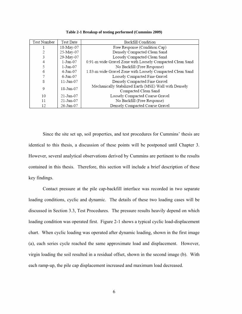
Table 2-1 Breakup of testing performed (Cummins 2009)
Since the site set up, soil properties, and test procedures for Cummins’ thesis are
identical to this thesis, a discussion of these points will be postponed until Chapter 3.
However, several analytical observations derived by Cummins are pertinent to the results
contained in this thesis. Therefore, this section will include a brief description of these
key findings.
Contact pressure at the pile cap-backfill interface was recorded in two separate
loading conditions, cyclic and dynamic. The details of these two loading cases will be
discussed in Section 3.3, Test Procedures. The pressure results heavily depend on which
loading condition was operated first. Figure 2-1 shows a typical cyclic load-displacement
chart. When cyclic loading was operated after dynamic loading, shown in the first image
(a), each series cycle reached the same approximate load and displacement. However,
virgin loading the soil resulted in a residual offset, shown in the second image (b). With
each ramp-up, the pile cap displacement increased and maximum load decreased.
6
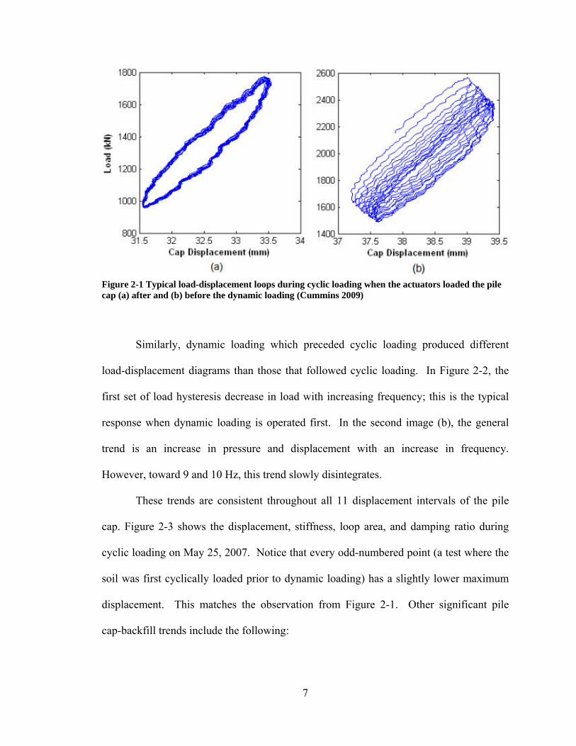
Figure 2-1 Typical load-displacement loops during cyclic loading when the actuators loaded the pile cap (a) after and (b) before the dynamic loading (Cummins 2009)
Similarly, dynamic loading which preceded cyclic loading produced different
load-displacement diagrams than those that followed cyclic loading. In Figure 2-2, the
first set of load hysteresis decrease in load with increasing frequency; this is the typical
response when dynamic loading is operated first. In the second image (b), the general
trend is an increase in pressure and displacement with an increase in frequency.
However, toward 9 and 10 Hz, this trend slowly disintegrates.
These trends are consistent throughout all 11 displacement intervals of the pile
cap. Figure 2-3 shows the displacement, stiffness, loop area, and damping ratio during
cyclic loading on May 25, 2007. Notice that every odd-numbered point (a test where the
soil was first cyclically loaded prior to dynamic loading) has a slightly lower maximum
displacement. This matches the observation from Figure 2-1. Other significant pile
cap-backfill trends include the following:
7
• System stiffness increased as the pile cap was displaced into the backfill
• System stiffness was greater when cyclic preceded dynamic loading
• Load-displacement hysteresis generally increased with forcing frequency
• Damping ratio generally remained constant with pile cap displacement
Figure 2-2 Typical load-displacement loops during dynamic loading when the shaker loaded the pile cap (a) before and (b) after the cyclic loading (Cummins 2009)
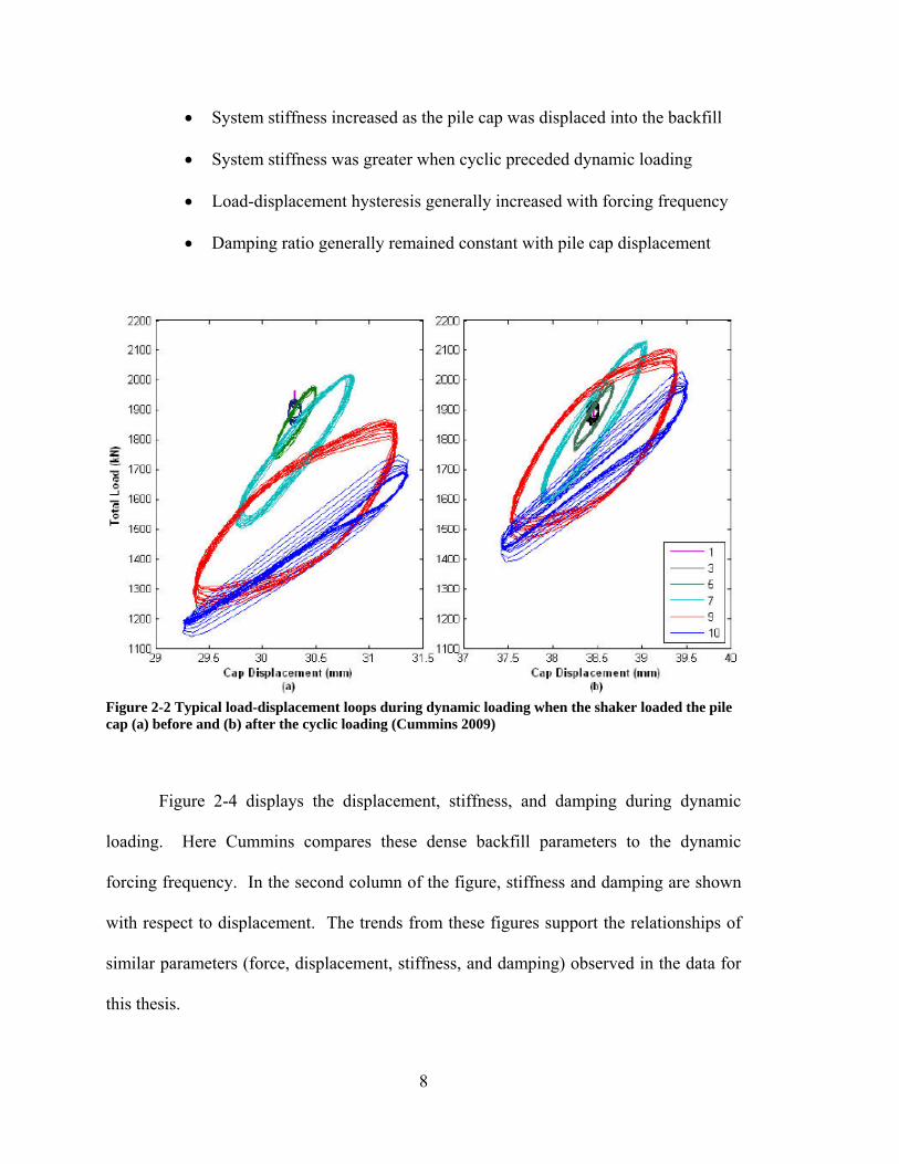
Figure 2-4 displays the displacement, stiffness, and damping during dynamic
loading. Here Cummins compares these dense backfill parameters to the dynamic
forcing frequency. In the second column of the figure, stiffness and damping are shown
with respect to displacement. The trends from these figures support the relationships of
similar parameters (force, displacement, stiffness, and damping) observed in the data for
this thesis.
8

Figure 2-3 Cyclic displacement amplitude, stiffness, loop area, and damping during loading of densely compacted sand backfill (Cummins 2009)
9
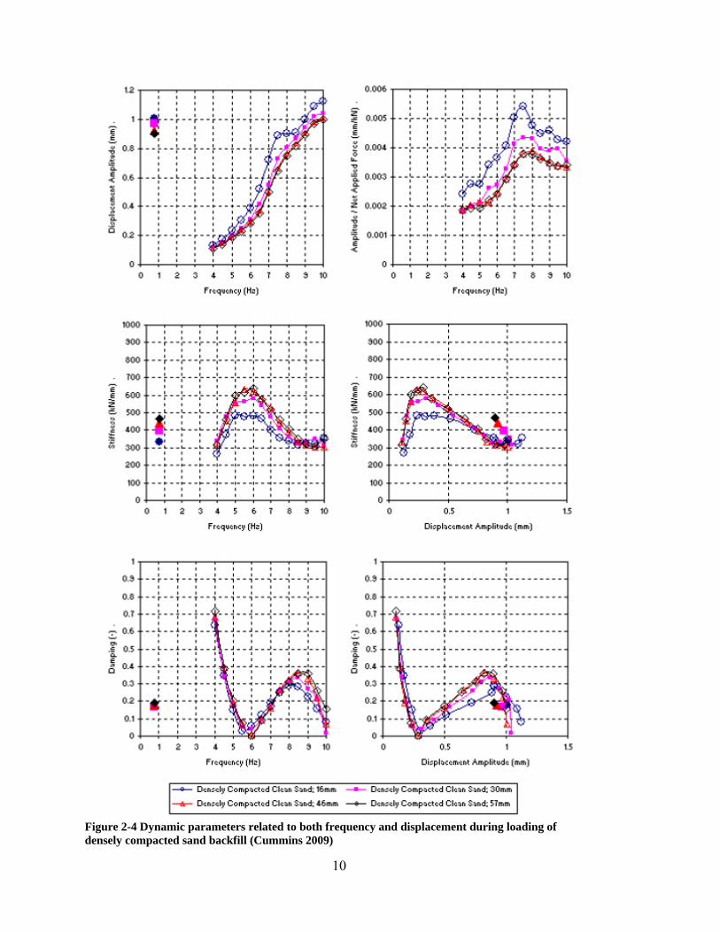
Figure 2-4 Dynamic parameters related to both frequency and displacement during loading of densely compacted sand backfill (Cummins 2009)
10
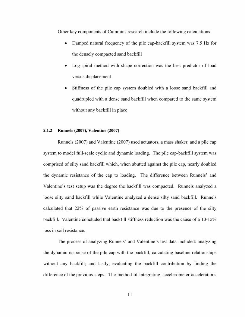
Other key components of Cummins research include the following calculations:
• Damped natural frequency of the pile cap-backfill system was 7.5 Hz for
the densely compacted sand backfill
• Log-spiral method with shape correction was the best predictor of load
versus displacement
• Stiffness of the pile cap system doubled with a loose sand backfill and
quadrupled with a dense sand backfill when compared to the same system
without any backfill in place
2.1.2 Runnels (2007), Valentine (2007)
Runnels (2007) and Valentine (2007) used actuators, a mass shaker, and a pile cap
system to model full-scale cyclic and dynamic loading. The pile cap-backfill system was
comprised of silty sand backfill which, when abutted against the pile cap, nearly doubled
the dynamic resistance of the cap to loading. The difference between Runnels’ and
Valentine’s test setup was the degree the backfill was compacted. Runnels analyzed a
loose silty sand backfill while Valentine analyzed a dense silty sand backfill. Runnels
calculated that 22% of passive earth resistance was due to the presence of the silty
backfill. Valentine concluded that backfill stiffness reduction was the cause of a 10-15%
loss in soil resistance.
The process of analyzing Runnels’ and Valentine’s test data included: analyzing
the dynamic response of the pile cap with the backfill; calculating baseline relationships
without any backfill; and lastly, evaluating the backfill contribution by finding the
difference of the previous steps. The method of integrating accelerometer accelerations
11
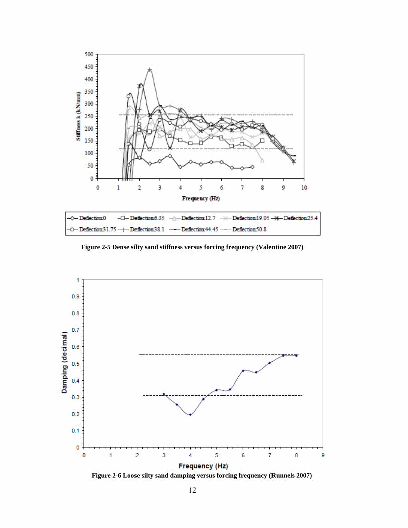
Figure 2-5 Dense silty sand stiffness versus forcing frequency (Valentine 2007)
Figure 2-6 Loose silty sand damping versus forcing frequency (Runnels 2007)
12
(which was adopted into this thesis and will be explained in Section 4.1.1.2.1) was the
primary source for retrieving accurate dynamic displacements. Similar to the test set-up
for this thesis, string potentiometers were installed, but their readings were skewed during
shaker testing due to dynamic vibrations.
Correlations produced by Runnels (2007) and Valentine (2007) validate the trends
realized in this thesis. Backfill stiffness was observed to generally decrease with
increasing frequency. This relationship is shown in Figure 2-5 at various pile cap
displacement intervals. As the pile cap is dynamically loaded, stiffness of the pile
cap-backfill system generally decreases after the stiffness is fully activated which occurs
between 1 to 3 Hz. Inversely, damping increased with increasing frequency. Figure 2-6
shows this comparison from Runnels (2007).
2.2 Static and Cyclic Passive Earth Pressure
2.2.1 Duncan and Mokwa (2001)
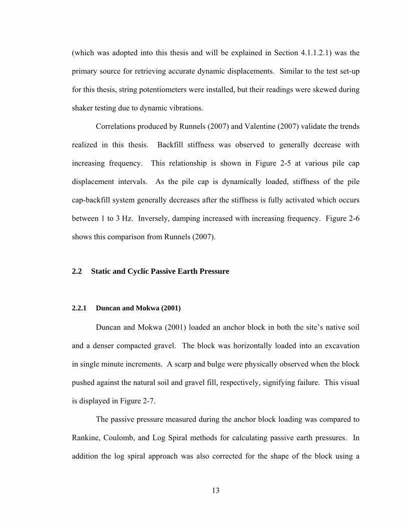
Duncan and Mokwa (2001) loaded an anchor block in both the site’s native soil
and a denser compacted gravel. The block was horizontally loaded into an excavation
in single minute increments. A scarp and bulge were physically observed when the block
pushed against the natural soil and gravel fill, respectively, signifying failure. This visual
is displayed in Figure 2-7.
The passive pressure measured during the anchor block loading was compared to
Rankine, Coulomb, and Log Spiral methods for calculating passive earth pressures. In
addition the log spiral approach was also corrected for the shape of the block using a
13
method produced by Brinch Hansen (1966) based off of research performed by
Ovesen (1964). This correction considers a 3D shape effect on mobilizing pressure.
In Table 2-2 these four methods for computing passive pressure are compared to
the actual measured pressure. The Coulomb theory and Log Spiral method are similar in
their associated passive pressure results. However, the 3D corrected log spiral
approximates the earth passive pressure closer to the pressures measured by Duncan and
Mokwa than any other method reviewed.
Duncan and Mokwa concluded that passive pressure is dependent on the
displacement of a structure, the backfill stiffness, and the structure-backfill interface
friction and adhesion. In addition, accounting for the shape of the structure more
accurately estimates the calculated passive pressure.
Figure 2-7 Soil failure type during testing various backfill conditions (Duncan and Mokwa 2001)
14

Table 2-2 Comparison of passive resistances (kips) (Duncan and Mokwa 2001)
2.2.2 Cole (2003), Cole and Rollins (2006)
Several theories analyzing the maximum displacement necessary to fully mobilize
passive earth resistance were compiled by Cole and Rollins. One objective of their
research was to derive a method for calculating the maximum passive pressure fully
mobilized behind a pile cap. Four backfill materials were used: clean sand, silty sand,
fine gravel, and course gravel. Cole and Rollins suggest that displacements ranging 3.0
to 5.2% of the pile cap height will allow the maximum passive earth pressures to develop.
Sources, namely the U.S. Navy (1986), Caltran (2001), and Duncan and
Mokwa (2001), produced original methods and models to contrast passive force versus
deflection. The comparison between these sources is displayed in Figure 2-8. The
hyperbolic model produced by Duncan and Mokwa (2001) most closely aligned with the
pressure measured by Cole and Rollins (2006). However, generally these three methods
underestimated the measured passive resistance.
During cyclic loading, passive force at the pile cap-backfill interface decreased.
This reduction stemmed from a gap which formed between the backfill and the pile cap.
15
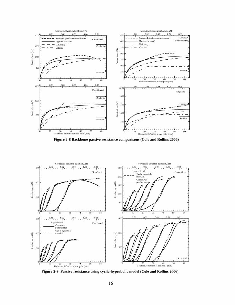
Figure 2-8 Backbone passive resistance comparisons (Cole and Rollins 2006)
Figure 2-9 Passive resistance using cyclic-hyperbolic model (Cole and Rollins 2006)
16
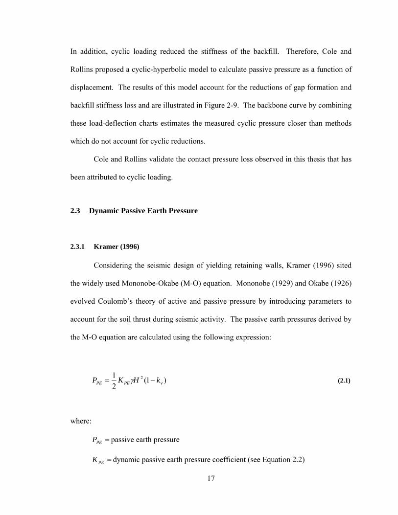
In addition, cyclic loading reduced the stiffness of the backfill. Therefore, Cole and
Rollins proposed a cyclic-hyperbolic model to calculate passive pressure as a function of
displacement. The results of this model account for the reductions of gap formation and
backfill stiffness loss and are illustrated in Figure 2-9. The backbone curve by combining
these load-deflection charts estimates the measured cyclic pressure closer than methods
which do not account for cyclic reductions.
Cole and Rollins validate the contact pressure loss observed in this thesis that has
been attributed to cyclic loading.
2.3 Dynamic Passive Earth Pressure
2.3.1 Kramer (1996)
Considering the seismic design of yielding retaining walls, Kramer (1996) sited
the widely used Mononobe-Okabe (M-O) equation. Mononobe (1929) and Okabe (1926)
evolved Coulomb’s theory of active and passive pressure by introducing parameters to
account for the soil thrust during seismic activity. The passive earth pressures derived by
the M-O equation are calculated using the following expression:
)1(21 2
vPEPE kHKP −= γ (2.1)
where:
=PEP passive earth pressure
=PEK dynamic passive earth pressure coefficient (see Equation 2.2)
17

=γ unit weight of soil
=H height of the retaining wall
=vk vertical acceleration seismic coefficient
This equation is the Coulomb theory for passive pressure with the addition of a
dynamic passive earth pressure coefficient (KPE) and a vertical acceleration seismic
coefficient (kv). KPE may be further defined by the following equation:
2
2
2
)cos()cos()sin()sin(1)cos(coscos
)(cos
⎥⎦
⎤⎢⎣
⎡
−+−−++
−+−
−+=
θβψθδψβφφδψθδθψ
ψθφPEK (2.2)
where:
=φ backfill friction angle
=θ inclination of structure measured from vertical
=ψ seismic inertia angle
=δ interface friction angle
=β slope inclination angle
The equivalent from these two equations is a single resultant force representing
both the static and dynamic force contributions. The forces resulting in an equivalent
passive resultant are shown in Figure 2-10 as a free body diagram. The M-O equation
18
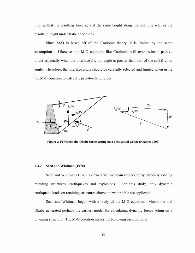
implies that the resulting force acts at the same height along the retaining wall as the
resultant height under static conditions.
Since M-O is based off of the Coulomb theory, it is limited by the same
assumptions. Likewise, the M-O equation, like Coulomb, will over estimate passive
thrust especially when the interface friction angle is greater than half of the soil friction
angle. Therefore, the interface angle should be carefully selected and limited when using
the M-O equation to calculate pseudo-static forces.
Figure 2-10 Mononobe-Okabe forces acting on a passive soil wedge (Kramer 1996)
2.3.2 Seed and Whitman (1970)
Seed and Whitman (1970) reviewed the two main sources of dynamically loading
retaining structures: earthquakes and explosions. For this study, only dynamic
earthquake loads on retaining structures above the water table are applicable.
Seed and Whitman began with a study of the M-O equation. Mononobe and
Okabe generated perhaps the earliest model for calculating dynamic forces acting on a
retaining structure. The M-O equation makes the following assumptions:
19

• Retaining structure is above the water table
• Backfill is a homogenous, dry, cohesionless material
• Retaining wall yields enough to fully mobilize active and passive pressures
• Backfill acts as a rigid body such that seismic accelerations are consistent
• Resultant force acts at the same height as the static resultant force
In the M-O equation, the horizontal force is extremely sensitive to several terms
which, therefore, must be accurately determined. For example, the soil friction angle will
increase the horizontal force acting on the retaining wall by 50 percent in only a 10
degree shift. Another condition which largely affects the horizontal force on the wall is
the backfill slope. In comparison with static horizontal force calculated by Coulomb, the
dynamic horizontal force is sometimes three times higher with a similar backfill slope.
Other variables, such as the vertical acceleration coefficient (kv), do not largely
affect the calculated dynamic force. According to Seed and Whitman, this kv factor may
be neglected for seismic analysis.
Seed and Whitman cited the efforts of Jacobsen (1939) and Matsuo (1941) in
verifying their calculated M-O forces. In both of these reports, the resultant force was
described as acting on the retaining structure a distance of 2/3 the wall height from the
base of the wall.
2.3.3 Richards and Elms (1979)
Richards and Elms (1979) discussed gravity retaining walls during seismic
activity calling the review of Seed and Whitman (1970) “misleading and
20
unconservative.” They cite investigatory observations following the 1968 Inangahua,
New Zealand earthquake. From the observed damages, estimates of the driving force to
wall resistance ratio were determined as 3.5 to 4.5 times the normal static conditions.
Mononobe-Okabe, as referred to in Seed and Whitman, would predict only 2.5 times the
static condition.
When reviewing the M-O equation, Richards and Elms (1979) concurred with
Seed and Whitman (1970) on several levels. Insignificant factors include the wall
friction angle and the vertical seismic acceleration. As seismic intensity increases, the
contribution of both of these terms becomes negligible. Critical parameters include the
backfill slope and the soil friction angle. Richards and Elms differ from Seed and
Whitman by assuming a uniform pressure distribution during seismic activity. Thus, the
resultant force would act at a height ratio H/2 from the base of the wall as opposed to
Seed and Whitman’s proposed 2H/3 ratio.
As Richards and Elms continued their discussion, the importance of including the
weight of the resisting structure was recommended. By combining the M-O equation and
Newmark’s sliding block analogy, this study derived an allowable displacement
approach. Included in this approach is a maximum wall displacement with an associated
vertical acceleration limit.
During shaking when passive conditions exist, Richards and Elms write “the wall
and the soil undoubtedly act together since the threshold acceleration for relative motion
at the base would be very large indeed” (Richards and Elms 1979). This thesis finds
observations contrary to that statement.
21

2.3.4 Whitman (1990)
Whitman (1990) reviewed the M-O equation in an effort to simplify the design of
gravity retaining walls. In addition, the use of the allowable permanent displacement
method by Richards and Elms was discussed (1979).
The article began with a review of the M-O equation. The M-O equation is based
off of several assumptions. Inherent to the Coulomb equations for pressure, the backfill
must deform thus mobilizing the interface shear resistance. Another assumption is that
the soil must be uniform. The backfill must also propagate accelerations consistently and
evenly.
Whitman then transitioned into a discussion on gravity retaining structures. He
concluded that simple walls less than 30 ft (9.14 m) and that are not restrained from
outward movements may be effectively designed using the M-O equation.
2.3.5 Ostadan and White (1997)
The objective of Ostadan and White’s report was to develop a method for
calculating lateral seismic pressure for building foundations. Criticizing the overuse of
the M-O equation with its several limitations, the reports says, “The M-O method is one
of the most abused methods in geotechnical practice”(Ostadan and White 1997). For
building foundations, the M-O equation would be inappropriate. Thus a model for
estimating seismic pressures was developed which matched the following conditions:
• Building walls are non-yielding and are confined to displacements
• Design motion is fully considered not just a single peak ground acceleration
22

• Material damping, Poisson’s ratio, soil density, and shearwave velocity are
considered
• Soil nonlinearity may be considered
• Soil-building interactions are taken into account by analyzing foundation rocking
motion, embedment, and soil motion and geometry
Ostadan and White divide their approach into two fundamental categories: firm
soil layer foundation and deep soil sites. The later takes into account the rocking motion
of a structure. Each situation was modeled by the Computer Program SASSI. During the
firm layer analysis, a vertical propagating shearwave was induced at the rock layer.
Pressure amplification was observed as the frequency of the system matched the soil
column’s natural frequency. In every variation of Ostadan and White’s analysis, the
maximum amplification of the pressure was at this natural frequency.
At shallow depths the soil tends to soften during dynamic motions. This occurs
due to the relatively low confining pressure on the soil material. For this thesis softening
of the soil is a significant parameter in calculating soil pressures. Since this thesis studies
a single pile cap, all of the backfill may be considered shallow and, therefore, subject to
softening.
Ostadan and White developed a polynomial equation to represent the soil
distribution acting on the structure. This equation, represented in terms of y, is the
following:
5432 14.859.2425.2848.1505.50015.)( yyyyyyp +−+−+−= (2.3)
23
where:
y = Y/H
Y = distance from bottom of the wall
H = height of the wall
The simplified method purposed by Ostadan and White, which output is
Equation 2.3, was compared to the computer model from SASSI. This new method
yields a range of results largely dependent on the input frequency.
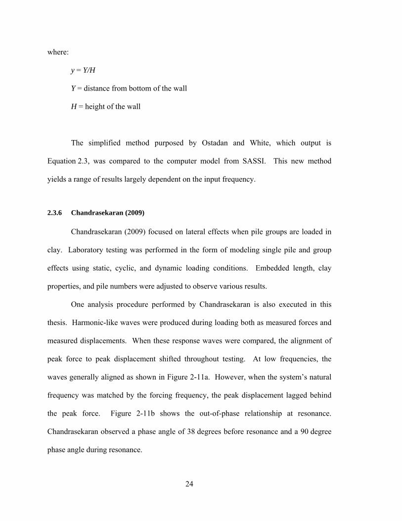
2.3.6 Chandrasekaran (2009)
Chandrasekaran (2009) focused on lateral effects when pile groups are loaded in
clay. Laboratory testing was performed in the form of modeling single pile and group
effects using static, cyclic, and dynamic loading conditions. Embedded length, clay
properties, and pile numbers were adjusted to observe various results.
One analysis procedure performed by Chandrasekaran is also executed in this
thesis. Harmonic-like waves were produced during loading both as measured forces and
measured displacements. When these response waves were compared, the alignment of
peak force to peak displacement shifted throughout testing. At low frequencies, the
waves generally aligned as shown in Figure 2-11a. However, when the system’s natural
frequency was matched by the forcing frequency, the peak displacement lagged behind
the peak force. Figure 2-11b shows the out-of-phase relationship at resonance.
Chandrasekaran observed a phase angle of 38 degrees before resonance and a 90 degree
phase angle during resonance.
24
Figure 2-11 Phase lag between force and displacement (a) before resonance (b) after resonance (Chandrasekaran 2009)
25

26
The method by which these phase angles were derived is used later in this thesis.
Two harmonic waves are first compared during similar time interval. The time interval
between peaks is then calculated and divided by the time wavelength of either harmonic
wave. This proportion multiplied by 360 degrees yields the phase angle offset between
the comparable harmonic measurements.
3 Methods of Testing
The testing for this thesis was part of a larger group of tests performed during
May and June of 2007. Some on-site structures were constructed in previous years in
connection with other research testing. Likewise, subsurface conditions were explored in
prior years. All of the test data analyzed in the following chapters was recorded on
May 25, 2007. This chapter specifically outlines methods for retrieving data on the
25th of May and relevant data compiled from previous research.
3.1 Site Characterization
For this research, testing was performed at a site located 300 m north of the
control tower at the Salt Lake City International Airport, in Salt Lake City, Utah. Figure
3-1 displays a satellite image of the testing site in relation to the Salt Lake City
International Airport.
The site, generally open and flat, is covered by approximately 1.5 m of imported
clayey to silty sand and gravel fill. Exploration of subsurface material was primarily
conducted in 1995 by Peterson (1996). Testing included Cone Penetration Tests,
Pressuremeter Tests, and laboratory tests. The locations of subsurface tests at the site are
illustrated in Figure 3-2. Figure 3-3 displays an idealized soil profile formulated using
these investigatory tests. The test site may be generally described as silt and clay layers
27

occasionally interrupted by sand layers. For a more detailed review of the site and its
subsurface characteristics reference Peterson (1996), Rollins et al. (2005a, 2005b),
Christensen (2006), and Taylor (2006). Because this research is independent of the
surrounding native soil, the subsurface conditions will not be belabored.
During testing, the water table on site was less than 10 m below the ground
surface. Pumps were used throughout the testing process to keep the water level at this
depth – beneath the pile cap and backfill.
Figure 3-1 Arial view of the site plan located 300 m north of the SLC Airport Control Tower
28
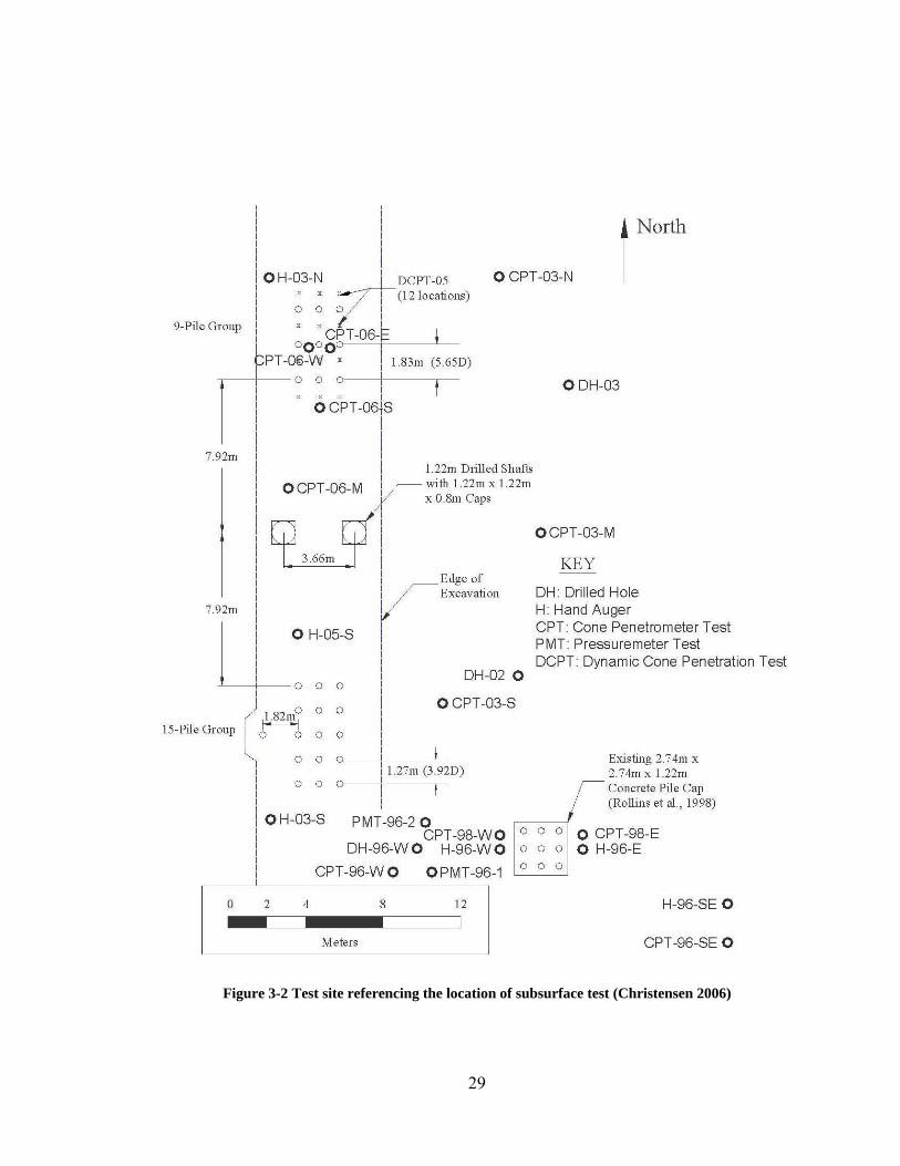
Figure 3-2 Test site referencing the location of subsurface test (Christensen 2006)
29

Figure 3-3 Idealized soil profile with CPT (Christensen 2006)
30
3.2 Test Components
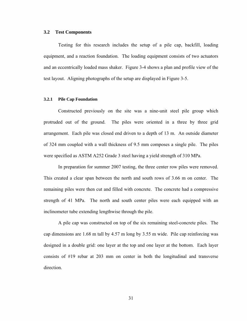
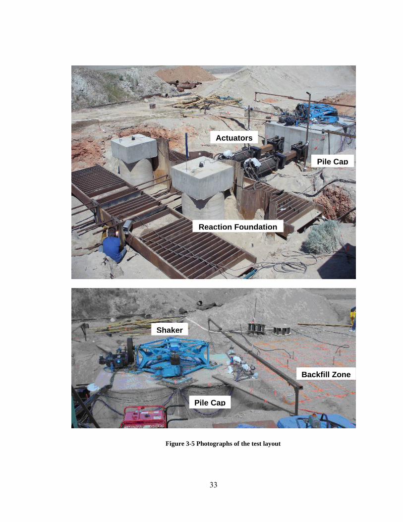
Testing for this research includes the setup of a pile cap, backfill, loading
equipment, and a reaction foundation. The loading equipment consists of two actuators
and an eccentrically loaded mass shaker. Figure 3-4 shows a plan and profile view of the
test layout. Aligning photographs of the setup are displayed in Figure 3-5.
3.2.1 Pile Cap Foundation
Constructed previously on the site was a nine-unit steel pile group which
protruded out of the ground. The piles were oriented in a three by three grid
arrangement. Each pile was closed end driven to a depth of 13 m. An outside diameter
of 324 mm coupled with a wall thickness of 9.5 mm composes a single pile. The piles
were specified as ASTM A252 Grade 3 steel having a yield strength of 310 MPa.
In preparation for summer 2007 testing, the three center row piles were removed.
This created a clear span between the north and south rows of 3.66 m on center. The
remaining piles were then cut and filled with concrete. The concrete had a compressive
strength of 41 MPa. The north and south center piles were each equipped with an
inclinometer tube extending lengthwise through the pile.
A pile cap was constructed on top of the six remaining steel-concrete piles. The
cap dimensions are 1.68 m tall by 4.57 m long by 3.55 m wide. Pile cap reinforcing was
designed in a double grid: one layer at the top and one layer at the bottom. Each layer
consists of #19 rebar at 203 mm on center in both the longitudinal and transverse
direction.
31

A A
1.5-m x 8.5-m I-BEAM(TYP)
SHEET PILE WALLSECTION AZ 18
(2) ACTUATORS 2.7 MN-EXTENSION 2.0 MN-CONTRACTION
1.2-m DIA. REINFORCEDCONCRETE SHAFTS
ECCENTRIC MASSSHAKER
0.3-m DIA.STEEL PILE(TYP)
3.4-m x 4.6-m x 1.7-mCONCRETE PILE CAP
7.0-m x 8.5-m BACKFILL AREA
North
SECTION A-A
LINE OF EXCAVATIONSLOPE 1V:3.5H
ECCENTRIC MASSSHAKER
1.5-m x 8.5-m I-BEAM(TYP OF 2)
SHEET PILE WALLSECTION AZ 18
GROUND LINE 0.3-m DIA.
STEEL PILE(TYP OF 6)
3.4-m x 4.6-m x 1.7-mCONCRETE PILE CAP
INDEPENDENTREFERENCEFRAME
(2) ACTUATORS 2.7 MN-COMPRESSION 2.0 MN-TENSION
1.2-m DIA. REINFORCEDCONCRETE SHAFTS
LEGEND OF SYMBOLS: STRING POTENTIOMETER
Figure 3-4 Plan and profile views of the test layout
32
Actuators
Pile Cap
Reaction Foundation
Shaker
Backfill Zone
Pile Cap
Figure 3-5 Photographs of the test layout
33
The pile cap encompasses the top 150 mm of each of the six remaining piles. A
5.49-m rebar cage connects the pile cap to each of the piles. The cage extends 1.47 m
into the cap and 4.02 m into each pile. Cage reinforcing is comprised of (6) #25 vertical
rebar encompassed by a 152 mm pitched #13 spiral rebar restraint. Incased by the pile
and pile cap, this cage ensures a rigid connection. The pile and pile cap now act as a
single, integral unit. Other connections extruding from the pile cap will be discussed in
Section 3.2.4 Loading Equipment.
3.2.2 Backfill
An excavation surrounded the pile cap. The excavation continued north of the
pile cap 5.2 m wide and 8.5 m long. Heavy equipment accessed the excavation via a
construction ramp with a vertical/horizontal slope of 1.0/3.5. This slope began 2.44 m
north of the pile cap. Between the slope and the pile cap, the excavated area was a
constant 2.16 m deep.
The excavation was filled with soil north of the pile cap. The backfill rested
against the northern face of the pile cap. For this thesis, well graded sand (SW),
designated using the Unified Soil Classification System (USGS), was used as backfill.
The sand was installed using 10-cm layers. Between each level, the backfill was
compacted.
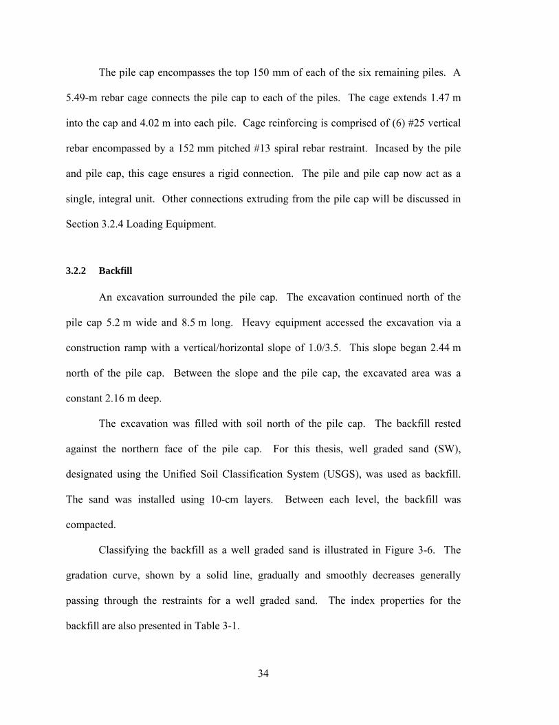
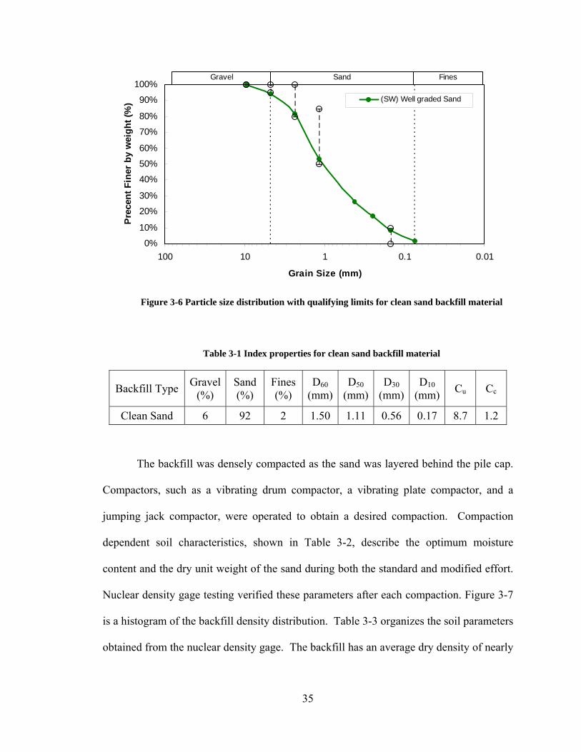
Classifying the backfill as a well graded sand is illustrated in Figure 3-6. The
gradation curve, shown by a solid line, gradually and smoothly decreases generally
passing through the restraints for a well graded sand. The index properties for the
backfill are also presented in Table 3-1.
34
0%
10%
20%
30%
40%
50%
60%
70%
80%
90%
100%
0.010.1110100
Grain Size (mm)
Prec
ent F
iner
by
wei
ght (
%) (SW) Well graded Sand
Gravel Sand Fines
Figure 3-6 Particle size distribution with qualifying limits for clean sand backfill material
Table 3-1 Index properties for clean sand backfill material
Backfill Type Gravel (%)
Sand (%)
Fines (%)
D60 (mm)
D50 (mm)
D30 (mm)
D10 (mm) Cu Cc
Clean Sand 6 92 2 1.50 1.11 0.56 0.17 8.7 1.2
The backfill was densely compacted as the sand was layered behind the pile cap.
Compactors, such as a vibrating drum compactor, a vibrating plate compactor, and a
jumping jack compactor, were operated to obtain a desired compaction. Compaction
dependent soil characteristics, shown in Table 3-2, describe the optimum moisture
content and the dry unit weight of the sand during both the standard and modified effort.
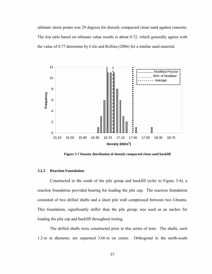
Nuclear density gage testing verified these parameters after each compaction. Figure 3-7
is a histogram of the backfill density distribution. Table 3-3 organizes the soil parameters
obtained from the nuclear density gage. The backfill has an average dry density of nearly
35
96% of the Modified Proctor maximum dry density and an average moist unit weight of
18.3 kN/m3.
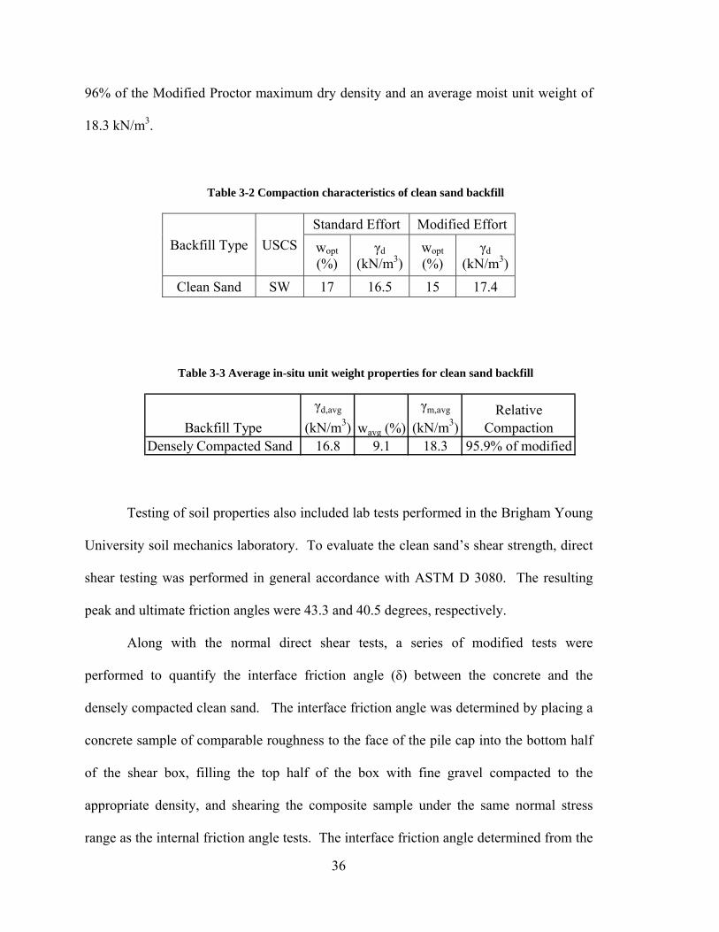
Table 3-2 Compaction characteristics of clean sand backfill
Backfill Type USCSStandard Effort Modified Effort wopt (%)
γd (kN/m3)
wopt (%)
γd (kN/m3)
Clean Sand SW 17 16.5 15 17.4
Table 3-3 Average in-situ unit weight properties for clean sand backfill
Backfill Type (kN/m ) wav
γd,avg 3
g (%) (kN/m ) CompactionDensely Compacted Sand 16.8 9.1 18.3 95.9% of modified
γm,avg 3
Relative
Testing of soil properties also included lab tests performed in the Brigham Young
University soil mechanics laboratory. To evaluate the clean sand’s shear strength, direct
shear testing was performed in general accordance with ASTM D 3080. The resulting
peak and ultimate friction angles were 43.3 and 40.5 degrees, respectively.
Along with the normal direct shear tests, a series of modified tests were
performed to quantify the interface friction angle (δ) between the concrete and the
densely compacted clean sand. The interface friction angle was determined by placing a
concrete sample of comparable roughness to the face of the pile cap into the bottom half
of the shear box, filling the top half of the box with fine gravel compacted to the
appropriate density, and shearing the composite sample under the same normal stress
range as the internal friction angle tests. The interface friction angle determined from the
36
ultimate stress points was 29 degrees for densely compacted clean sand against concrete.
The δ/φ ratio based on ultimate value results is about 0.72, which generally agrees with
the value of 0.77 determine by Cole and Rollins (2006) for a similar sand material.
0
2
4
6
8
10
12
15.10 15.50 15.90 16.30 16.70 17.10 17.50 17.90 18.30 18.70
Density (kN/m3)
Freq
uenc
y
………….. Modified Proctor________ 95% of Modified- - - - - - - - Average
Figure 3-7 Density distribution of densely compacted clean sand backfill
3.2.3 Reaction Foundation
Constructed to the south of the pile group and backfill (refer to Figure 3-4), a
reaction foundation provided bearing for loading the pile cap. The reaction foundation
consisted of two drilled shafts and a sheet pile wall compressed between two I-beams.
This foundation, significantly stiffer than the pile group, was used as an anchor for
loading the pile cap and backfill throughout testing.
The drilled shafts were constructed prior to this series of tests. The shafts, each
1.2 m in diameter, are separated 3.66 m on center. Orthogonal to the north-south
37
direction of testing, these shafts are the structure behind static and dynamic loading of the
pile cap. When constructed, the two shafts were capped with a 1.22 m by 1.22 m by
0.61 m concrete cap. Beneath the cap the west shaft extends downward a length of
16.82 m. The east shaft was constructed to 21.35 m deep. Each shaft was reinforced
using #36 bars with #16 spiral stirrups. From the top to 10.67 m deep, (18) #36
reinforcement bars were installed with the stirrups on a 75-mm pitch. At 10.67 m half of
the rebar was discontinued and the stirrup pitch increased to 300 mm. A 120-mm clear
cover was maintained between the surface of the concrete and the outermost steel
reinforcement. The concrete compressive strength is 41-MPa for both shafts.
An AZ-18 sheet piling was installed flush to the drilled shafts. This wall, 12.2 m
in height, provides additional stiffness to the drilled shafts. The sheet pile wall was made
from ASTM A-572, Grade 50 steel, and was pushed to a depth of 10.24 m to 10.85 m
below the excavation’s surface using a vibratory hammer.
Two steel I-beams pinch the sheet pile wall to the existing drilled shafts. Each
beam extends 8.53 m running parallel to the sheet pile wall in an east-west direction. The
beams, 1626 mm by 406 mm, lay flat on either side of the shaft-sheet pile system. The
beams web stiffeners, groups of 16 on each end and a group of 8 in the center, protect the
beam from crippling.
The two steel beams, sandwiching the drilled shafts and sheet pile wall, are
strapped to each other by (8) 64-mm high-strength, treaded bars. After post tensioning to
45 kN, the entire reaction foundation acts as an amalgamated unit 1.22 m south of the
pile-pile cap system.
38

3.2.4 Loading Equipment
Between the pile cap and the reaction foundation, two hydraulic actuators were
oriented north to south. Each actuator has the capacity to produce up to 2.7 MN of
horizontal force as it expands and contracts. The actuators were attached to the center of
the south face of the pile cap using four treaded bars which protruded from the concrete
cap at the time of construction. This connection was designed so that the actuator would
perform as an integral unit with the pile cap. The south end of the actuator was attached
to the reaction foundation at the four treaded post-tensioned ties discussed above.
Rotational joints on the actuator heads ensured moment free connections. Extension
arms were added to the actuator so that the loading equipment could span between the
reaction foundation and the pile cap system.
Dynamic loading on the pile cap was stimulated using an eccentrically loaded
mass shaker. This mechanism imitates earthquakes through quick rotations of an off-
balanced weight. Steel blocks may be added to the shaker in 0.08-kN increments to
increase the force produced by the shaker. Adjusting the placement of these weights will
also modify the force exuded by the shaker. The further away the weight is from the
center of rotation the greater the shaker force. This offset distance is referred to as the
eccentricity. The force the shaker produces is directly related to both the weight and its
eccentricity in addition to the number of rotations per time. This equation may be written
as follows:
2)(04016.0 fWRF ⋅⋅= (3.1)
39

where:
F = force produced by shaker, kN
WR = moment, weight multiplied by the its eccentricity, kN-cm
f = frequency, Hz
The term 0.04016 is an empirically derived factor specific to the model of shaker
used. For this research, the shaker climbed to a maximum frequency of 10 Hz with
weights offset to produce a 110.97 kN-cm moment. This configuration generated a
maximum force of 446 kN. This force acted in the north-south direction, perpendicular
to major supports and parallel to loading from the actuator.
The shaker’s attachment to the pile cap was similar to the actuator’s connection to
the cap. In this case, treaded bars were positioned in the pile cap protruding from the top,
centered. The shaker was supported directly on top of the cap and bolted in place. Thus,
the shaker acted integral with the pile cap.
3.2.5 Instrumentation
An independent reference frame was constructed to provide an unmoving datum.
Steel beams spanning the excavation were anchored in concrete unaffected by the
actuator. The reference frame dissected the space between the pile cap and the stiff
reaction frame directly above the actuators. Tension guide cables were used to stabilize
the frame from any movement. However, during dynamic loading the ground in which
the independent reference frame was anchored vibrated thus invalidating the
measurements of instruments attached to the frame.
40
Mounted on the independent reference frame attaching to the pile cap face were
four string potentiometers. Sting potentiometers measure real-time displacements by
gauging the expansion or retraction of a cable connecting the potentiometer to the object
under observation. In this manner, relative displacements could be evaluated during
testing. Seven additional string potentiometers were attached to the pile cap and staked
into the backfill.
Attached to the top of the pile cap in the corners, the center, and along the
northern edge were triaxial accelerometers. These instruments measure accelerations in
real-time. Accelerometers were independent from the reference frame which is critically
important during dynamic loading when the reference frame began to vibrate.
Accelerometers were also strategically positioned in the backfill at 0.61, 1.83, and 3.66 m
north of the pile cap.
Earth pressure cells were used to measure contact pressures between the pile cap
and the backfill. The Geokon Model 3510 Earth Pressure Cell was chosen for its ability
to accurately measure dynamic soil pressures. This stainless steel, circular model was
designed with two plates, a thick back plate and a thin upper plate. The thick back plate
is designed to be in direct contact of the structure (ie. pile cap) and resist flexure through
the earth cell induced by the dynamically loaded structure. This back plate protects
against erroneous point loads from being measured by the pressure cell. The thin plate
responds to the change in pile cap-backfill interface pressure. A depiction of the Geokon
Model 3510 is shown in Figure 3-8. The pressure plates were also designed with a semi-
conductor pressure transducer, as opposed to a vibrating wire transducer, to accurately
measure pressures during dynamic loading.
41

Pressure CellTransducer Housing Instrument Cable
(4 pair, 22 AWG)
Side View
Top View
9" 230 mm
Mounting Lugs (4 places)
Thin Pressure Sensitive Plate
Figure 3-8 Geokon Model 3510 contact pressure cell (Geokon 2004)
Figure 3-9 Pressure plates constructed on the north face of the pile cap
42

Six Geokon 3510 Earth Pressure Cells were wet set flush into the north face of the
pile cap during construction. The pressure plates were staggered within the central
portion of the pile cap face located at depths of 0.14, 0.42, 0.7, 0.98, 1.26, 1.54 m from
the top of the cap. Figure 3-9 shows the northern face of the pile cap with the pressure
plates in position before the backfill was in place.
Lastly, a painted grid was outlined on the top of the backfill’s surface after the
backfill was in place and compacted according to specifications. The grid, spaced with
0.61-m square nodes, provided a means for visual inspection. The vertical displacements
at each node were measured using traditional surveying methods and equipment.
3.3 Test Procedures
The pile cap with densely compacted sand backfill in place was loaded statically,
cyclically, and dynamically. Each type of loading was completed according to the testing
procedures described in this section.
After placement of backfill materials, the hydraulic load actuators were used to
load and displace the pile cap to its initial target displacement level. After a several-
second pause to manually record verification data, the actuators were used to apply 15
small amplitude displacement cycles (typically on the order of 2 mm (single amplitude)
at 0.75 Hz). After returning the actuators to their starting pre-cycling positions, the
lengths of the actuators were fixed, causing each actuator to act as a strut between the
reaction and test foundations. The shaker was then activated and a dynamic stepped-
ramp loading was applied. The ramped loading consisted of dwelling on a specified
frequency for 15 cycles and then ramping as fast as possible to the next dwell frequency.
43

The dwell frequencies ranged from 1 to 10 Hz, in 0.5 Hz increments. Afterwards, the
shaker was allowed to ramp back down. The duration of shaker operation was typically
about 3½ minutes, which includes the ramp up and the ramp down to the stopped
position.
Figure 3-10 displays a typical shaker frequency verses time relationship during
dynamic loading. The dwelling periods are illustrated as the plateaus between increasing
frequencies. As the frequency increases, the cycles occupy less time; therefore, the
plateau lengths decrease as dynamic loading progresses. Noise at the beginning and
ending of the dynamic loading are mechanical and ignored in the analysis.
Figure 3-10 Typical forcing frequency verses time during dynamic loading
44
After cyclic and dynamic loading were completed the backfill was visually
inspected, the actuators were extended again to push the pile cap to the next displacement
level. Upon reaching the target displacement level, rather than having the actuators cycle
first as was performed previously, the shaker was used with the actuator lengths fixed.
Dynamic shaker loading was operated with the same prescribed frequencies as before.
After the shaker loading was completed, the actuators applied their cyclic loading
as previously described. Hence, the use of cyclic actuator loads and dynamic shaker
loads was alternated between each target displacement level throughout the testing
program until the maximum target displacement was reached.
This process was repeated, expanding the actuator arms and then loading the pile
cap with the actuators and shaker (alternating loading order at each pile cap displacement
interval), for 11 displacement intervals. Throughout the entire test, data was continually
being recorded. Measurements were made with a computer data acquisition system at a
sampling rate of 200 samples per second (sps). The test data is organized under one of
two categories. Notation for data during the dynamic loading is classified as a “Shake”
followed by the pile cap displacement interval. The cyclic loading measurements are
categorized as “Series” followed by the pile cap displacement interval.
Table 3-4 displays the organization of data in categories of Series and Shakes
according to various pile cap displacements. For example, if backfill accelerations were
recorded during dynamic loading while the actuators were locked in place at 16 mm, then
these accelerations would be categorized as results in Shake 4. The fourth displacement
interval encompasses all results from both Shake 4 (dynamic loading) and Series 4
(cyclic loading).
45
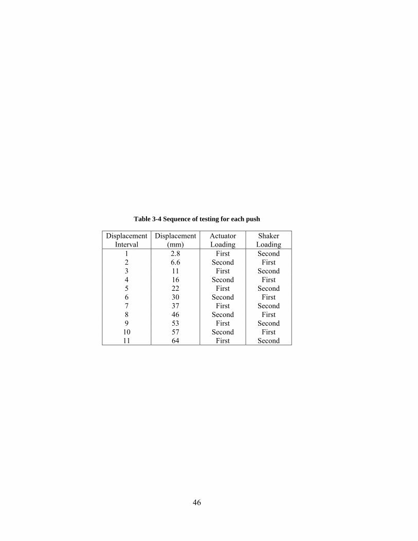
Table 3-4 Sequence of testing for each push
Displacement Interval
Displacement (mm)
Actuator Loading
Shaker Loading
1 2.8 First Second 2 6.6 Second First 3 11 First Second 4 16 Second First 5 22 First Second 6 30 Second First 7 37 First Second 8 46 Second First 9 53 First Second
10 57 Second First 11 64 First Second
46

4 Methods of Analysis
This chapter describes the measurements collected from the lateral load test
performed on the pile cap with dense sand backfill in place. The methods used to reduce
measured data will be discussed, and the analytical methods used to interpret the reduced
data will also be presented. The details of the testing procedure were presented
previously in Section 3.3. Subsequent chapters will discuss the interpreted results.
Focus has been placed on pile cap displacement interval eight and nine for two
primary reasons. First, previous research has concluded that displacements of 2 to 5% of
the pile cap height are required to fully mobilize soil passive earth pressures (NCHRP
2008). For this pile cap (1.68 m deep), 2 and 5% equate to displacement levels of 33.6
and 84 mm. Push 8 and Push 9 begin at a pile cap displacement level of 46 mm (2.7%)
and 53 mm (3.15%), respectively. In this case, inspection of the load-displacement curve
by Cummins (2009) determined that passive pressure was fully mobilized at a
displacement-to-pile-cap-height ratio of approximately 0.03, which corresponds to a
displacement of about 50 mm. Hence, the displacement levels associated with the eighth
displacement interval and subsequent displacement intervals are in the range where
passive earth pressures are expected to be fully mobilized. At lower displacement levels,
passive pressure is largely a function of displacement, and cyclic and dynamic loading
effects are difficult to separate. Additionally, even and odd numbered displacement
47
intervals reflect different loading conditions. During the even-numbered displacement
intervals, the dynamic loading from the shaker is performed first as opposed to the
odd-numbered displacement intervals during which the cyclic loading from the actuator
is performed first. Because of this alternating order, data obtained during the second half
of the loading sequence (cyclic loading if even and dynamic loading if odd) are based off
of non-virgin (i.e., previously loaded and affected) soil conditions.
4.1 Data Reduction
4.1.1 Pile Cap Displacements
The data collected by string potentiometers during cyclic loading conditions will
be reviewed first followed by displacements collected by string potentiometers during
dynamic loading conditions. In addition, accelerations measured by accelerometers were
reduced into displacements. The reduction and importance of these acceleration based
displacements will be presented.
With respect to sign convention, the string potentiometer data has been adjusted
such that positive pile cap displacement values represent northward displacements, in the
direction of the actuator thrust during static loading. When accelerometer data was
recorded, positive values represented accelerations in the north direction. After
integrating these accelerations to determine displacements, positive values likewise
represented displacements in the north direction. However, positive displacements
measured by string potentiometers at first represented displacements in the south
direction. String potentiometer signs were reversed to make the displacements
compatible with the accelerometer data (the relationship between accelerations and
48
displacements will be explained at a later point in this section). To assure the correctness
and consistency of the displacement data from both string potentiometers and
accelerometers, the pressure plate data was examined during the static pushes as well as
the slowly applied cyclic loadings. During the slow actuator loadings, dynamic effects
are expected to be minimal and the measured pressures should increase as the pile cap
moves northward into the soil backfill.
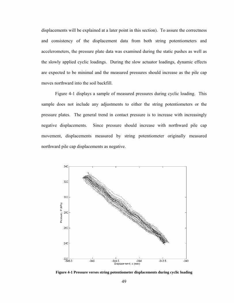
Figure 4-1 displays a sample of measured pressures during cyclic loading. This
sample does not include any adjustments to either the string potentiometers or the
pressure plates. The general trend in contact pressure is to increase with increasingly
negative displacements. Since pressure should increase with northward pile cap
movement, displacements measured by string potentiometer originally measured
northward pile cap displacements as negative.
Figure 4-1 Pressure verses string potentiometer displacements during cyclic loading
49
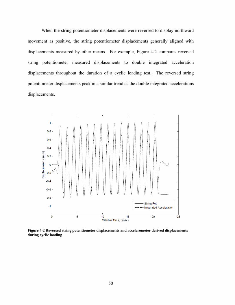
When the string potentiometer displacements were reversed to display northward
movement as positive, the string potentiometer displacements generally aligned with
displacements measured by other means. For example, Figure 4-2 compares reversed
string potentiometer measured displacements to double integrated acceleration
displacements throughout the duration of a cyclic loading test. The reversed string
potentiometer displacements peak in a similar trend as the double integrated accelerations
displacements.
Figure 4-2 Reversed string potentiometer displacements and accelerometer derived displacements during cyclic loading
50

4.1.1.1 Displacements during Cyclic Loading
Measured displacements during cyclic loading exhibited similar displacement
patterns at each pile cap displacement interval. Figure 4-3 and Figure 4-4 display cyclic
loading displacements during Series 8 and Series 9, respectively. In each figure, the load
series are represented with an initial displacement corresponding to the displacement
interval of the pile cap (refer to Table 3-4).
A typical cyclic loaded displacement pattern begins with a brief quiet period.
Then the actuators start to expand and retract according to the prescribed test procedure.
The actuators cycle 15 times shown as 15 distinct peaks in the corresponding figures.
The wavelength between peaks is approximately 1.33 seconds which agrees with the
prescribed actuator cyclic frequency of 0.75 Hz. After the actuators have expanded and
contracted 15 times the retracted position was held constant before the pile cap was
returned to its displacement interval position.
While the general pattern of cyclic displacements remains constant at each pile
cap displacement interval, a few distinct differences may be highlighted by the
comparison of Series 8 and Series 9. During Series 8 the pile cap displaces between 45.2
and 47 mm north from its unloaded position (prior to the first displacement interval).
This is a 1.8 mm spread between the maximum and minimum displacement. During
Series 9 the pile cap displacements range from 52.2 to 54.2 mm north of the unloaded
pile cap position, a 2 mm spread throughout loading.
The difference between Series 8 and Series 9 displacement spread is largely
attributed to the residual offset occurring during each cyclically loaded displacement
interval. The pile cap is being displaced further north into the backfill with each actuator
51
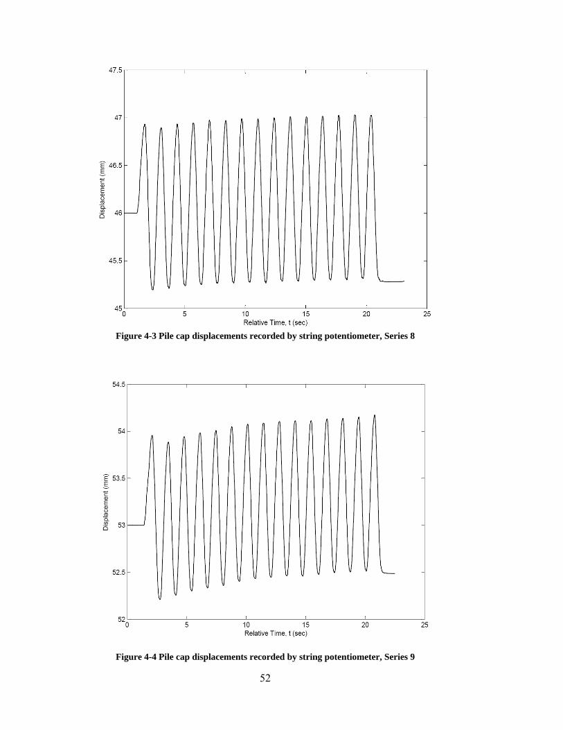
Figure 4-3 Pile cap displacements recorded by string potentiometer, Series 8
Figure 4-4 Pile cap displacements recorded by string potentiometer, Series 9
52

cycle. This offset may be observed in both Figure 4-3 and Figure 4-4 as the displacement
peaks gradually become increasingly positive. The displacements in Series 8 and
Series 9 offset approximately 0.12 and 0.29 mm, respectively. This expected difference
originates from the alternating loading sequence for even and odd displacement intervals.
4.1.1.2 Displacements during Dynamic Loading
Like cyclic displacements, typical dynamically loaded pile cap displacements
have correlating trends and patterns. Figure 4-5 and Figure 4-6 show a string
potentiometer measured displacements during Shake 8 and Shake 9, respectively. The
pile cap at the beginning of Shake 8 has previously been displaced 46 mm into the
backfill from the unloaded pile cap position. Shake 9 begins at a displacement of 53 mm
from the unloaded pile cap position.
As the eccentrically loaded mass shaker began to ramp up, the dynamic forces
jerked the pile cap back and forth. At first this motion minimally displaced the pile cap.
As the test progressed, the increasing bandwidth (the difference between minimum and
maximum displacement at a specific time) on the figures signifies increasing pile cap
displacement. Once the shaker began to ramp down, the displacement bandwidth
decreased until the dynamic loading concluded.
During dynamic loading, the ground surrounding the excavation shook including
the independent reference frame. Since string potentiometers measure the distance
between the pile cap and the independent reference frame, erratic peaks and dips in
Figure 4-5 and Figure 4-6 are likely caused by the vibratory reference frame position.
Therefore, local displacements measured by string potentiometers during dynamic
loading at every displacement interval are considered erroneous.
53

Frequency
Displacement
Figure 4-5 Pile cap displacement time history recorded by string potentiometer, Shake 8
Frequency
Displacement
Figure 4-6 Pile cap displacement time history recorded by string potentiometer, Shake 9
54

One relationship measured from the string potentiometers during dynamic loading
that is considered accurate is the total offset of the pile cap throughout dynamic loading.
The position of the independent reference frame before and after dynamic loading did not
change. However, neither Figure 4-5 nor Figure 4-6 show the pile cap ending in its
starting position. Figure 4-5, for example, shows the final pile cap location 48.4 mm
north from the unloaded pile cap position despite the pile cap being displaced only
46 mm north at the beginning of the dynamic loading. This means that during Shake 8
the pile cap displaced an additional 2.4 mm north. Likewise, during Shake 9, the pile cap
displaced an additional 1.16 mm north.
4.1.1.2.1 Integrating Accelerations
Dynamic accelerations on the pile cap are directly related to the shaker frequency.
Figure 4-7 is one example of the pile cap accelerations during dynamic loading. In this
figure, the accelerations are symmetrical about the x-axis origin signifying that
accelerations induced by the mass shaker were approximately equal in both the north and
south direction. The peak acceleration of the pile cap occurs just before 150 seconds
which corresponds to the maximum shaker frequency, 10 Hz. The cap maximum
acceleration occurs at 10 Hz during dynamic loading at every pile cap displacement
interval.
One method to obtain accurate displacements during dynamic loading is to double
integrate accelerations. Accelerations were integrated using MatLab programming by the
following process:
1. Raw data accelerations taken at 0.005 second intervals (200 sps) were uploaded
2. Accelerations were processed using a forward and backward FIR filter
55

3. Velocities were derived by summing trapezoidal areas using time periods of
0.005 seconds
4. Velocity units were converted into inches per second
5. Velocities were processed using a forward and backward FIR filter
6. Displacements were derived by summing trapezoidal areas using time periods of
0.005 seconds
7. Data file was exported with displacements in inches
Figure 4-7 Typical pile cap accelerations time history due to dynamic loading, Shake 8
A finite impulse response (FIR) filter was used for its unique ability to filter
displacements without shifting the time interval of those displacements. Unlike a typical
Butterworth filter which attempts to remove peaks by mathematically flat-lining data, a
56

FIR filter eliminates potential group delay or phase distortion. Using the FIR filter and
the trapezoidal integration method, pile cap accelerometer accelerations were integrated
into displacements for all eleven displacement intervals.
A typical plot of integrated acceleration displacements is shown in Figure 4-8.
This specific figure was created using displacements calculated by double integrating
Shake 8 accelerations. The displacements directly follow the accelerations pattern of the
mass shaker which was presented in Figure 4-7. Displacement magnitudes are symmetric
about the pile cap position at the beginning of the dynamic loading. Therefore, the
acceleration based displacements do not account for any residual offset (i.e., the
displacements end at the same position as the displacements begin at the start of the
Figure 4-8 Typical displacements calculated from double integration of accelerometer data
57
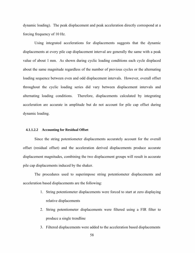
dynamic loading). The peak displacement and peak acceleration directly correspond at a
forcing frequency of 10 Hz.
Using integrated accelerations for displacements suggests that the dynamic
displacements at every pile cap displacement interval are generally the same with a peak
value of about 1 mm. As shown during cyclic loading conditions each cycle displaced
about the same magnitude regardless of the number of previous cycles or the alternating
loading sequence between even and odd displacement intervals. However, overall offset
throughout the cyclic loading series did vary between displacement intervals and
alternating loading conditions. Therefore, displacements calculated by integrating
acceleration are accurate in amplitude but do not account for pile cap offset during
dynamic loading.
4.1.1.2.2 Accounting for Residual Offset
Since the string potentiometer displacements accurately account for the overall
offset (residual offset) and the acceleration derived displacements produce accurate
displacement magnitudes, combining the two displacement groups will result in accurate
pile cap displacements induced by the shaker.
The procedures used to superimpose string potentiometer displacements and
acceleration based displacements are the following:
1. String potentiometer displacements were forced to start at zero displaying
relative displacements
2. String potentiometer displacements were filtered using a FIR filter to
produce a single trendline
3. Filtered displacements were added to the acceleration based displacements
58
To further explain this process the steps will be illustrated, compared, and contrasted
during Shake 8 and Shake 9.
Figure 4-9 and Figure 4-10 show the same string potentiometer displacements
presented in Figure 4-5 and Figure 4-6. The displacements were translated to initially
begin at zero. The same erratic peaks and dips caused by the vibrating independent
reference frame still exist. The relative offset remains the same – 2.4 mm during Shake 8
and 1.3 mm during Shake 9.
Figure 4-12 and Figure 4-13 display the second step in determining accurate
displacements during the dynamic loading. A FIR filter, depicted in Figure 4-11, was
processed through the string potentiometer displacements. The outcome was a single
trendline which has a zero phase distortion. At this point in the process the string
Figure 4-9 Cap displacement time history based on string potentiometer data, Shake 8
59

Figure 4-10 Cap displacement time history based on string potentiometer data, Shake 9
Figure 4-11 Trendline showing overall offset in sample of cap displacement data during dynamic loading
60

Figure 4-12 Overall trend of displacement data based on string potentiometer data, Shake 8
Figure 4-13 Overall trend of displacement data based on string potentiometer data, Shake 9
61

potentiometer displacements begin at zero displacement, maintain their respective offsets
(2.4 and 1.3 mm for Shake 8 and Shake 9, respectively), and are represented as a
trendline.
The displacements originating from accelerometer measurements are then
combined with the trendline displacements, resulting in the displacement time histories
shown in Figure 4-14 and Figure 4-15. These figures resemble the typical displacements
shown in Figure 4-8 but now including 2.4 and 1.3 mm offsets between the beginning
and ending of the dynamic loading as measured by the string potentiometers during
Shake 8 and Shake 9, respectively. These combined displacements represent the pile cap
displacements as they are believed to have occurred during testing.
Figure 4-14 Cap displacement time history based on accelerometer-derived displacements corrected for offset, Shake 8
62
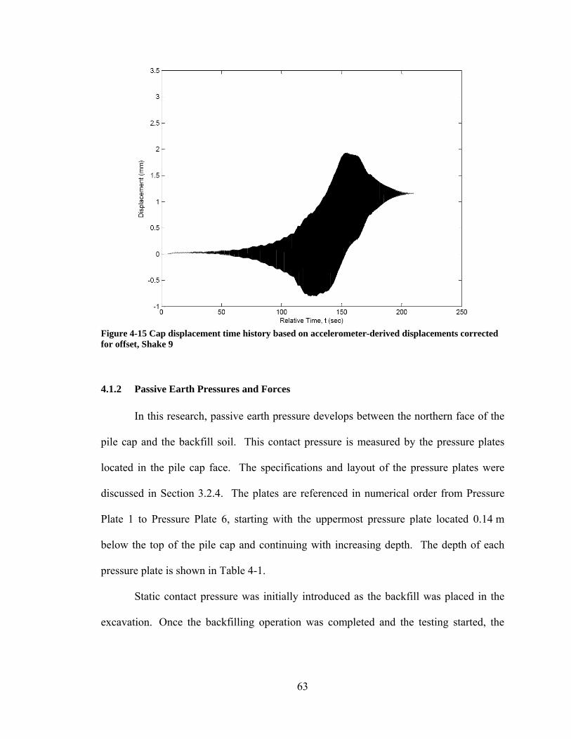
Figure 4-15 Cap displacement time history based on accelerometer-derived displacements corrected for offset, Shake 9
4.1.2 Passive Earth Pressures and Forces
In this research, passive earth pressure develops between the northern face of the
pile cap and the backfill soil. This contact pressure is measured by the pressure plates
located in the pile cap face. The specifications and layout of the pressure plates were
discussed in Section 3.2.4. The plates are referenced in numerical order from Pressure
Plate 1 to Pressure Plate 6, starting with the uppermost pressure plate located 0.14 m
below the top of the pile cap and continuing with increasing depth. The depth of each
pressure plate is shown in Table 4-1.
Static contact pressure was initially introduced as the backfill was placed in the
excavation. Once the backfilling operation was completed and the testing started, the
63

Table 4-1 Depth to pressure plates
Plate Number Depth (m)1 0.12 0.43 0.74 0.95 1.26 1.5
420864
actuators displaced the pile cap into the backfill. With each pile cap displacement
interval, static pressure increased. The resulting pressure distributions corresponding to
the end of each static push are shown in Figure 4-16. As shown in the figure, the
measured pressures generally increased with depth. This aligns with accepted static soil
pressure distribution theories. However, the deepest pressure plate (referred to as
Pressure Plate 6 in this thesis) does not follow this trend.
A few possibilities may explain the seemingly questionable measurements from
Pressure Plate 6. One possibility could be that the backfill was not firmly compacted
against the plate. The measured pressure would be unexpectedly low with minimal
contact area between the soil and pressure plate. However, since pressures measured by
Pressure Plate 6 increase initially (between the first and second pile cap displacement
interval) this explanation is not likely. Another explanation for the low pressures might
be that the pile cap rotated during loading (the top of the pile cap displacing further into
the backfill than the bottom of the pile cap). Douglas and Davis (1964) state that a 0.1 o
rotation (2.8 mm for this pile cap) would be sufficient for the bottom pressure plate to
measure no increase in pressure. However, the observed cap rotation during testing was
significantly less than the 0.1 rotation needed to produce such a significant decrease in
pressure at the bottom of the pile cap. It is possible, and most probable, that the pressure
o
64
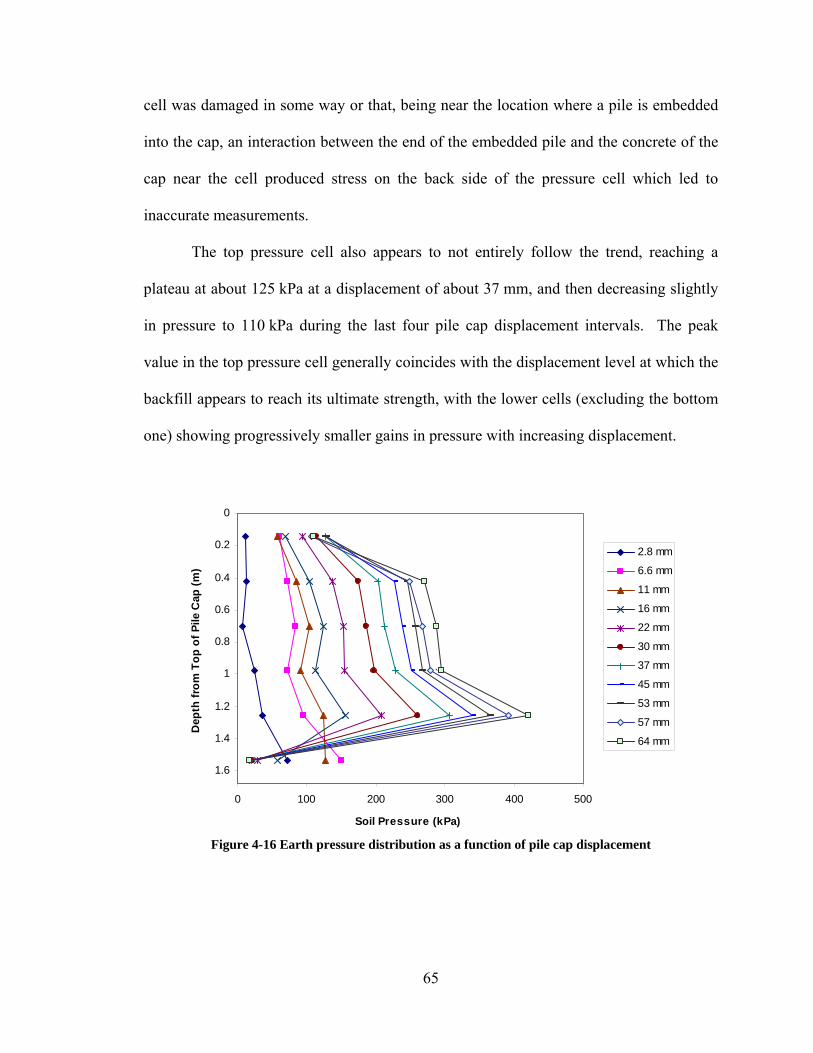
cell was damaged in some way or that, being near the location where a pile is embedded
into the cap, an interaction between the end of the embedded pile and the concrete of the
cap near the cell produced stress on the back side of the pressure cell which led to
inaccurate measurements.
The top pressure cell also appears to not entirely follow the trend, reaching a
plateau at about 125 kPa at a displacement of about 37 mm, and then decreasing slightly
in pressure to 110 kPa during the last four pile cap displacement intervals. The peak
value in the top pressure cell generally coincides with the displacement level at which the
backfill appears to reach its ultimate strength, with the lower cells (excluding the bottom
one) showing progressively smaller gains in pressure with increasing displacement.
0
0.2
0.4
0.6
0.8
1
1.2
1.4
1.6
0 100 200 300 400 500
Soil Pressure (kPa)
Dep
th fr
om T
op o
f Pile
Cap
(m)
2.8 mm
6.6 mm
11 mm
16 mm
22 mm
30 mm
37 mm
45 mm
53 mm
57 mm
64 mm
`
Figure 4-16 Earth pressure distribution as a function of pile cap displacement
65

In addition to pressures measured under static loadings, pressures were measured
during both cyclic actuator loading and dynamic shaker loading. Figure 4-17 and Figure
4-18 show pressures measured by each pressure plate during Series 8 and Series 9,
respectively. The pressures, with the exception of those measured from Pressure Plate 6,
increase with depth, consistent with the trends observed during the static loadings. The
pressures during Series 9 do drift (i.e., decrease) slightly which directly corresponds to
the displacement offset observed during Series 9.
Figure 4-19 (Shake 8) and Figure 4-20 (Shake 9) display typical dynamic pressure
measured by the pressure plates. As the dynamic loading begins, pressure measurements
oscillate sinusoidally in response to the applied load. The pressure spread, the difference
between a local maxima and minima, slowly increases as each of the dynamic loading
sequences 7 Hz (120 seconds). Nearing 120 seconds there is a shift in the pressure trend.
At this point, the maximum pressures begin to decrease and the minimum pressures
decrease more rapidly than before. The spread of pressure continues to widen with
increasing shaker forcing frequency. For dynamic loading at both pile cap displacement
intervals (Shake 8 and Shake 9), the minimum pressure occurs around 150 seconds which
equates to a frequency of 10 Hz (the maximum shaker frequency). The maximum
pressure, however, does not occur at this point. After the minimum pressure, the spread
between maximum and minimum pressures decreases as the mass shaker ramps down.
This behavior is more fully examined and discussed in Chapter 6. Shake 8 exhibits
significant offset between starting pressures and ending pressures. Shake 9 shows only a
slight offset measured only by a few of the pressure plates. Recall that during Push 8 the
shaker loaded the pile cap first. Thus, during Shake 8 the pile cap and backfill were
66
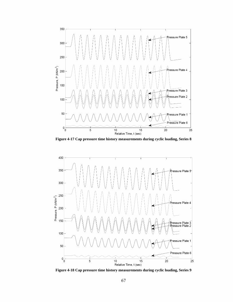
Figure 4-17 Cap pressure time history measurements during cyclic loading, Series 8
Figure 4-18 Cap pressure time history measurements during cyclic loading, Series 9
67
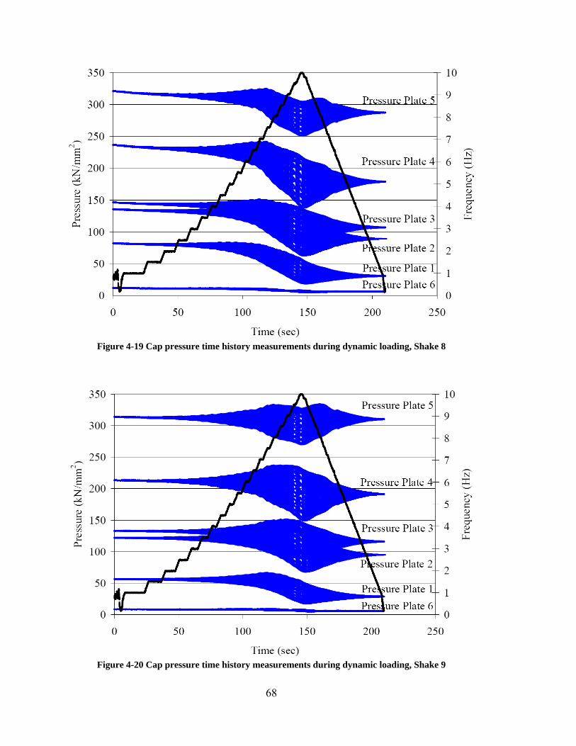
Figure 4-19 Cap pressure time history measurements during dynamic loading, Shake 8
Figure 4-20 Cap pressure time history measurements during dynamic loading, Shake 9
68
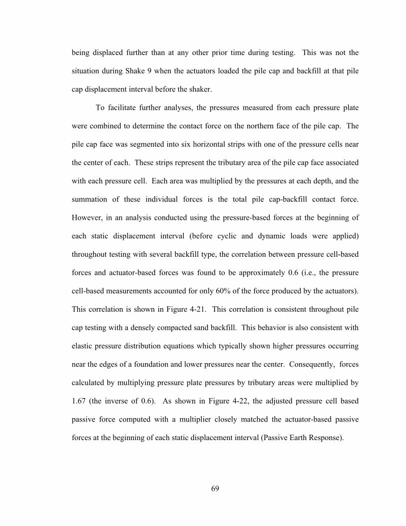
being displaced further than at any other prior time during testing. This was not the
situation during Shake 9 when the actuators loaded the pile cap and backfill at that pile
cap displacement interval before the shaker.
To facilitate further analyses, the pressures measured from each pressure plate
were combined to determine the contact force on the northern face of the pile cap. The
pile cap face was segmented into six horizontal strips with one of the pressure cells near
the center of each. These strips represent the tributary area of the pile cap face associated
with each pressure cell. Each area was multiplied by the pressures at each depth, and the
summation of these individual forces is the total pile cap-backfill contact force.
However, in an analysis conducted using the pressure-based forces at the beginning of
each static displacement interval (before cyclic and dynamic loads were applied)
throughout testing with several backfill type, the correlation between pressure cell-based
forces and actuator-based forces was found to be approximately 0.6 (i.e., the pressure
cell-based measurements accounted for only 60% of the force produced by the actuators).
This correlation is shown in Figure 4-21. This correlation is consistent throughout pile
cap testing with a densely compacted sand backfill. This behavior is also consistent with
elastic pressure distribution equations which typically shown higher pressures occurring
near the edges of a foundation and lower pressures near the center. Consequently, forces
calculated by multiplying pressure plate pressures by tributary areas were multiplied by
1.67 (the inverse of 0.6). As shown in Figure 4-22, the adjusted pressure cell based
passive force computed with a multiplier closely matched the actuator-based passive
forces at the beginning of each static displacement interval (Passive Earth Response).
69
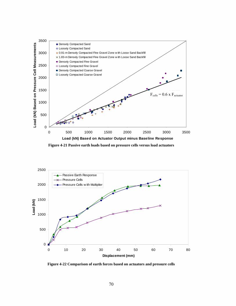
y = 0.5959x
0
500
1000
1500
2000
2500
3000
3500
0 500 1000 1500 2000 2500 3000 3500
Load (kN) Based on Actuator Output minus Baseline Response
Load
(kN
) Bas
ed o
n Pr
essu
re C
ell M
easu
rem
ents Densely Compacted Sand
Loosely Compacted Sand0.91-m Densely Compacted Fine Gravel Zone w ith Loose Sand Backfill1.83-m Densely Compacted Fine Gravel Zone w ith Loose Sand BackfillDensely Compacted Fine GravelLoosely Compacted Fine GravelDensely Compacted Coarse GravelLoosely Compacted Coarse Gravel
Figure 4-21 Passive earth loads based on pressure cells versus load actuators
0
500
1000
1500
2000
2500
0 10 20 30 40 50 60 70 80
Displacement (mm)
Load
(kN
)
Passive Earth ResponsePressure CellsPressure Cells w ith Multiplier
Figure 4-22 Comparison of earth forces based on actuators and pressure cells
Fcells = 0.6 x Factuator
70
4.2 Determination of Parameters
4.2.1 Backfill Stiffness
Stiffness is an inherent material and geometric property which resists external
forces. For this research, the pile cap activated the backfill stiffness as the cap was
displaced into the backfill. Stiffness may be measured with units of force per
displacement. The backfill stiffness may be calculated using the following equation:
cyclexxFF
k ⎟⎟⎠
⎞⎜⎜⎝
⎛−−
=minmax
minmax (4.1)
where:
k = backfill soil stiffness
F = contact force at maximum and minimum displacements of a cycle
x = maximum and minimum pile cap displacements of a cycle
Since stiffness is dependent on force and displacement, several force-
displacement figures are used in this research to identify trends in stiffness. On a force
verses displacement plot the slope of a trendline connecting force at minimum and
maximum displacements is the backfill stiffness.
4.2.2 Residual Offset
Displacement offset was previously observed during both cyclic and dynamic
loadings. During cyclic loading conditions, with each cycle the maximum displacement
increased (ie. the pile cap was displaced further north with each cycle). The difference
71
between displacement maxima during the 15 cycles provides continuous displacement
offset. Dynamic loading displacements were converted to a single trendline to show
continuous displacement offset (shown in Figure 4-12 and Figure 4-13). The difference
between the starting pile cap displacement and the pile cap displacement at the
conclusion of the dynamic loading is the total displacement offset or residual offset due
to dynamic loading.
Residual offset of the pile cap is directly responsible for partial reduction in
passive force between the pile cap and the backfill. During cyclic loading conditions the
difference between peak to peak force magnitudes provides continuous losses in force
which are at least in part associated with displacement offset. However, during dynamic
conditions continuous force losses associated with displacement offset may not simply be
computed using a filtered trendline of forces (as was previously done to compute
continuous displacement offset during dynamic loading). This is because several
different dynamic factors (in addition to displacement offset) contribute to losses in
dynamic contact force. Therefore, to isolate the loss in force due to displacement offset
that occurs throughout dynamic testing, force loss must be connected to displacement
offset.
One method to attribute the force loss due to displacement offset is to estimate the
force loss per unit of residual offset. This parameter may then be multiplied by the
displacement (relative to the displacement interval of the pile cap) at any time during
loading and yield a force loss due to the drifting displacements. The following equation
provides such a parameter:
72

12
12
xxFF
xF
Totaloffset
offset
−−
=⎟⎟⎠
⎞⎜⎜⎝
⎛ (4.2)
where:
offset
offset
xF
= force loss per unit of residual offset
1F = beginning measured force at pile cap-backfill interface
2F = ending measured force at pile cap-backfill interface
1x = beginning pile cap position
2x = ending pile cap position
4.2.3 Phase Angle
By definition, a phase angle is a numerical value denoting the degree in which
two moving objects are synchronized in motion. A phase angle of zero or 360 degrees
signifies that two objects are moving in the same direction at the same time. Inversely, a
phase angle of 180 degrees defines movement in opposing directions at similar time.
The relative movement of the backfill in relation to the pile cap during dynamic
loading may be observed by the separation of the pile cap and backfill displacement
amplitudes in relation to time. The following formula may be used to derive the phase
angle between the pile cap movement and the backfill movement:
cap
ntdisplacemesoilcap ttλ
φ max)(*360
−= (4.3)
73

where:
φ = phase angle, degrees
capt = time when maximum soil displacement occurs
soilt = time when maximum soil displacement occurs
capλ = pile cap wavelength in time
Alternatively, phase angles may be calculated through a comparison with
damping ratio. This relationship is introduced in basic structural dynamics (Chopra
2001). The phase angle increases as the forcing frequency surpasses the natural
frequency of the system subject to some degree of damping. This relationship is
described by the following equation:
( )( ) ⎥
⎥⎦
⎤
⎢⎢⎣
⎡
−= −
21
/1/2
tann
n
ωωωωζ
φ (4.4)
where:
=φ phase angle
=ζ damping ratio
=ω circular frequency
=nω natural circular frequency
However, the relationship between phase angle and damping assumes a linear stiffness.
In the analysis section of this thesis, the non-linearity of the backfill stiffness during
74
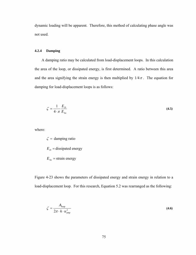
dynamic loading will be apparent. Therefore, this method of calculating phase angle was
not used.
4.2.4 Damping
A damping ratio may be calculated from load-displacement loops. In this calculation
the area of the loop, or dissipated energy, is first determined. A ratio between this area
and the area signifying the strain energy is then multiplied by 1/4π . The equation for
damping for load-displacement loops is as follows:
So
D
EE
πζ
⋅=
41
(4.5)
where:
=ζ damping ratio
=DE dissipated energy
=SoE strain energy
Figure 4-23 shows the parameters of dissipated energy and strain energy in relation to a
load-displacement loop. For this research, Equation 5.2 was rearranged as the following:
22 amp
loop
ukA⋅⋅
=π
ζ (4.6)
75
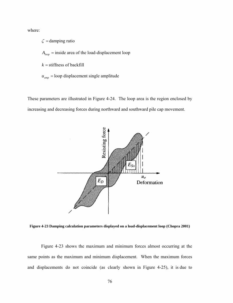
where:
=ζ damping ratio
=loopA inside area of the load-displacement loop
=k stiffness of backfill
=ampu loop displacement single amplitude
These parameters are illustrated in Figure 4-24. The loop area is the region enclosed by
increasing and decreasing forces during northward and southward pile cap movement.
Figure 4-23 Damping calculation parameters displayed on a load-displacement loop (Chopra 2001)
Figure 4-23 shows the maximum and minimum forces almost occurring at the
same points as the maximum and minimum displacement. When the maximum forces
and displacements do not coincide (as clearly shown in Figure 4-25), it is due to
76

Figure 4-24 Key parameters displayed on a load-displacement loop
Figure 4-25 Typical load displacement loop during dynamic loading at high frequency
Force at Maximum Displacement Maximum Force
77

damping. Stiffness (or the slope of the loop) is based on the peak displacements and
associated forces and not the peak (i.e., maximum) forces.
Figure 4-26 (after Chopra 2001) illustrates the relationship of viscous damping to
the force-displacement hysteresis loop which is a composite of both the damping and
stiffness forces. As derived from this figure and shown in the following equation, the
damping coefficient for the backfill can be calculated as:
( )amp
d
uf
c⋅
=ω
(4.7)
where:
=c damping coefficient
fd = force of the load-displacement loop at zero displacement
=ω circular forcing frequency (which is the circular frequency of the loop)
=ampu loop displacement amplitude
Figure 4-26 Damping component and combined stiffness and damping components (Chopera 2001)
78
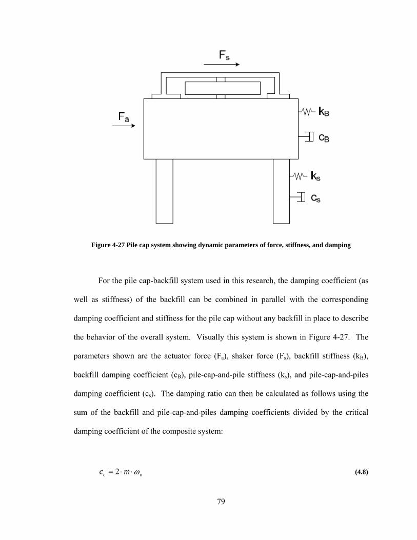
Figure 4-27 Pile cap system showing dynamic parameters of force, stiffness, and damping
For the pile cap-backfill system used in this research, the damping coefficient (as
well as stiffness) of the backfill can be combined in parallel with the corresponding
damping coefficient and stiffness for the pile cap without any backfill in place to describe
the behavior of the overall system. Visually this system is shown in Figure 4-27. The
parameters shown are the actuator force (Fa), shaker force (Fs), backfill stiffness (kB),
backfill damping coefficient (cB), pile-cap-and-pile stiffness (ks), and pile-cap-and-piles
damping coefficient (cs). The damping ratio can then be calculated as follows using the
sum of the backfill and pile-cap-and-piles damping coefficients divided by the critical
damping coefficient of the composite system:
nc mc ω⋅⋅= 2 (4.8)
79

where:
=cc critical damping coefficient of the composite system
m = mass of the system
=nω natural circular frequency of the composite system
80
5 Test Results
The development of passive earth pressure at the pile cap-backfill interface is
dependent on several factors. Some of these factors include backfill stiffness, cyclic
losses, damping, and the relative movement of the cap and backfill. Using the methods
discussed in Chapter 4, these parameters and their impact on the backfill soil pressure
will be assessed and presented in this chapter.
5.1 Backfill Stiffness
The backfill stiffness values calculated for both cyclic actuator loading and
dynamic shaker loading will be presented in this section. These stiffness values represent
reloading conditions rather than the initial loading stiffness associated with the static
displacement of the pile cap. The methods by which backfill stiffness was determined
were previously presented in Section 4.2.1.
Backfill stiffness generally remained constant during cyclic loading associated
with each particular displacement interval. This behavior is shown in Figure 5-1 for the
eighth pile cap displacement interval, where the force-displacement relationship is linear
and consistent during the 15 actuator loading cycles. As the actuator pushes the pile cap
into the soil, the cap and the soil are displaced to approximately one millimeter. When
this extension is reached, the actuators retract. As the actuators retract, the pile cap force
81
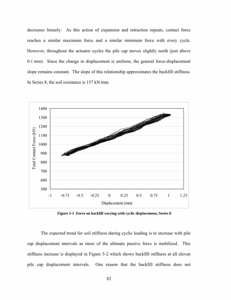
decreases linearly. As this action of expansion and retraction repeats, contact force
reaches a similar maximum force and a similar minimum force with every cycle.
However, throughout the actuator cycles the pile cap moves slightly north (just above
0.1 mm). Since the change in displacement is uniform, the general force-displacement
slope remains constant. The slope of this relationship approximates the backfill stiffness.
In Series 8, the soil resistance is 157 kN/mm.
500
600
700
800
900
1000
1100
1200
1300
1400
-1 -0.75 -0.5 -0.25 0 0.25 0.5 0.75 1 1.25
Displacement (mm)
Tota
l Con
tact
For
ce (k
N)
Figure 5-1 Force on backfill varying with cyclic displacement, Series 8
The expected trend for soil stiffness during cyclic loading is to increase with pile
cap displacement intervals as more of the ultimate passive force is mobilized. This
stiffness increase is displayed in Figure 5-2 which shows backfill stiffness at all eleven
pile cap displacement intervals. One reason that the backfill stiffness does not
82
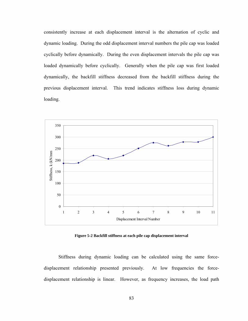
consistently increase at each displacement interval is the alternation of cyclic and
dynamic loading. During the odd displacement interval numbers the pile cap was loaded
cyclically before dynamically. During the even displacement intervals the pile cap was
loaded dynamically before cyclically. Generally when the pile cap was first loaded
dynamically, the backfill stiffness decreased from the backfill stiffness during the
previous displacement interval. This trend indicates stiffness loss during dynamic
loading.
0
50
100
150
200
250
300
350
1 2 3 4 5 6 7 8 9 10 1
Displacement Interval Number
Stiff
ness
, k (k
N/m
m
1
)
Figure 5-2 Backfill stiffness at each pile cap displacement interval
Stiffness during dynamic loading can be calculated using the same force-
displacement relationship presented previously. At low frequencies the force-
displacement relationship is linear. However, as frequency increases, the load path
83
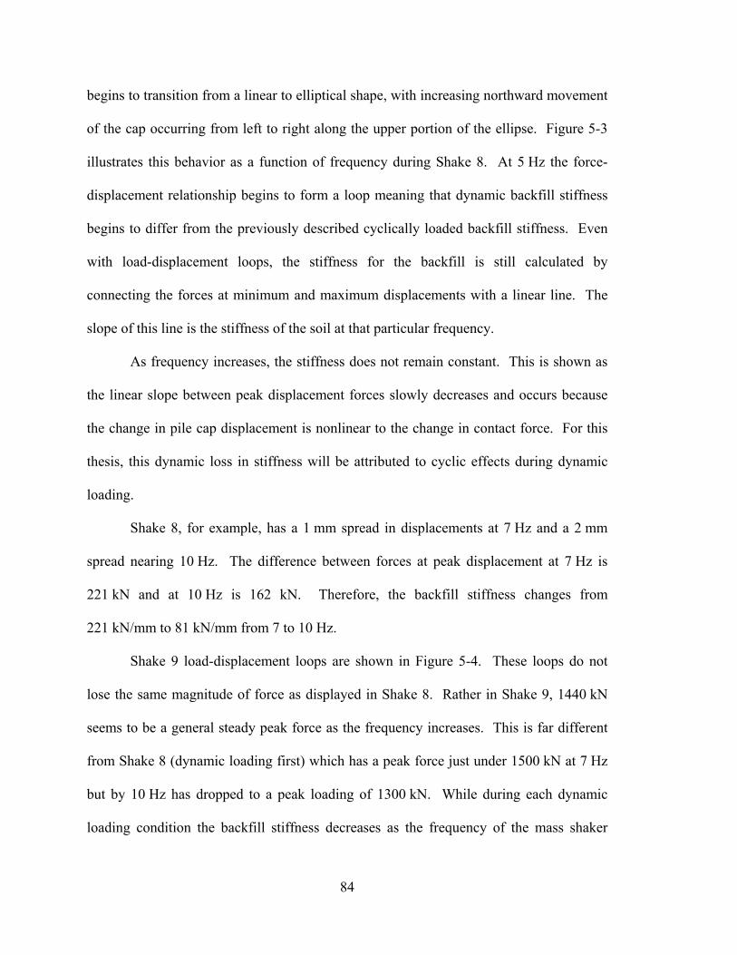
begins to transition from a linear to elliptical shape, with increasing northward movement
of the cap occurring from left to right along the upper portion of the ellipse. Figure 5-3
illustrates this behavior as a function of frequency during Shake 8. At 5 Hz the force-
displacement relationship begins to form a loop meaning that dynamic backfill stiffness
begins to differ from the previously described cyclically loaded backfill stiffness. Even
with load-displacement loops, the stiffness for the backfill is still calculated by
connecting the forces at minimum and maximum displacements with a linear line. The
slope of this line is the stiffness of the soil at that particular frequency.
As frequency increases, the stiffness does not remain constant. This is shown as
the linear slope between peak displacement forces slowly decreases and occurs because
the change in pile cap displacement is nonlinear to the change in contact force. For this
thesis, this dynamic loss in stiffness will be attributed to cyclic effects during dynamic
loading.
Shake 8, for example, has a 1 mm spread in displacements at 7 Hz and a 2 mm
spread nearing 10 Hz. The difference between forces at peak displacement at 7 Hz is
221 kN and at 10 Hz is 162 kN. Therefore, the backfill stiffness changes from
221 kN/mm to 81 kN/mm from 7 to 10 Hz.
Shake 9 load-displacement loops are shown in Figure 5-4. These loops do not
lose the same magnitude of force as displayed in Shake 8. Rather in Shake 9, 1440 kN
seems to be a general steady peak force as the frequency increases. This is far different
from Shake 8 (dynamic loading first) which has a peak force just under 1500 kN at 7 Hz
but by 10 Hz has dropped to a peak loading of 1300 kN. While during each dynamic
loading condition the backfill stiffness decreases as the frequency of the mass shaker
84
increases, the effect is far greater when the eccentrically loaded mass shaker is the first
loading device acting on the pile cap at the beginning of a load displacement interval.
Therefore, the effects of forcing frequency on stiffness loss should be observed during
Shake 8 as opposed to Shake 9.
Figure 5-3 Load displacement loops at 5, 6, and 7 Hz (column 1) and 8, 9, and 10 Hz (column 2), Shake 8
In Figure 5-5, Shake 8 backfill stiffness is displayed from 5 Hz to 10 Hz. At 5 Hz
the stiffness of the backfill is 321 kN/mm. By 10 Hz, the stiffness has dropped to 80 kN.
85

A linear relationship connects the data points between these two frequencies. At lower
frequencies the stiffness behaves similarly to cyclic conditions.
Figure 5-4 Load displacement loops at 5, 6, and 7 Hz (column 1) and 8, 9, and 10 Hz (column 2), Shake 9
5.2 Residual Offset
During dynamic loading, the pile cap displaced further north into the backfill such
that at the end of dynamic loading the pile cap was offset from its position at the
86
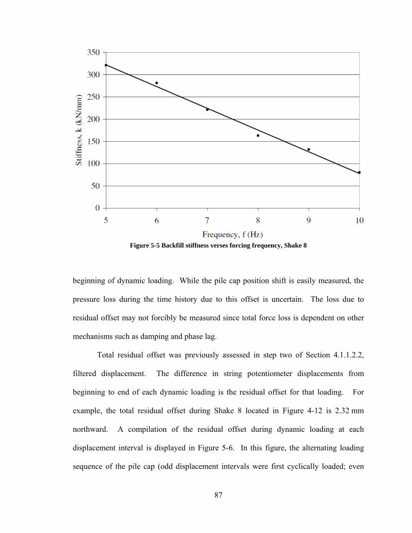
Figure 5-5 Backfill stiffness verses forcing frequency, Shake 8
beginning of dynamic loading. While the pile cap position shift is easily measured, the
pressure loss during the time history due to this offset is uncertain. The loss due to
residual offset may not forcibly be measured since total force loss is dependent on other
mechanisms such as damping and phase lag.
Total residual offset was previously assessed in step two of Section 4.1.1.2.2,
filtered displacement. The difference in string potentiometer displacements from
beginning to end of each dynamic loading is the residual offset for that loading. For
example, the total residual offset during Shake 8 located in Figure 4-12 is 2.32 mm
northward. A compilation of the residual offset during dynamic loading at each
displacement interval is displayed in Figure 5-6. In this figure, the alternating loading
sequence of the pile cap (odd displacement intervals were first cyclically loaded; even
87

displacement intervals were first dynamically loaded) significantly affects the pile cap
offset. For reasons stated previously, the backfill displaced more during dynamic
loadings which preceded cyclic loadings than dynamic loadings which followed cyclic
loadings at a particular displacement interval. The offset significantly increased between
the dynamic loading during the fifth and sixth displacement intervals. Increasing residual
offset occurs because the force applied to the backfill increases initially with loading
sequence. However, as the passive force develops the change in force begins to decrease.
Therefore, after the sixth displacement interval the pile cap offset slowly diminishes
(ignoring alternating loading effect).
In subsequent comparisons, the dynamic passive force acting upon the pile cap
face will need to be compared to the static force during dynamic loading. Since the static
force could not be measured during dynamic loading (due to dynamic effects), it is
Figure 5-6 Pile cap offset during dynamic loading at each pile cap displacement interval
88
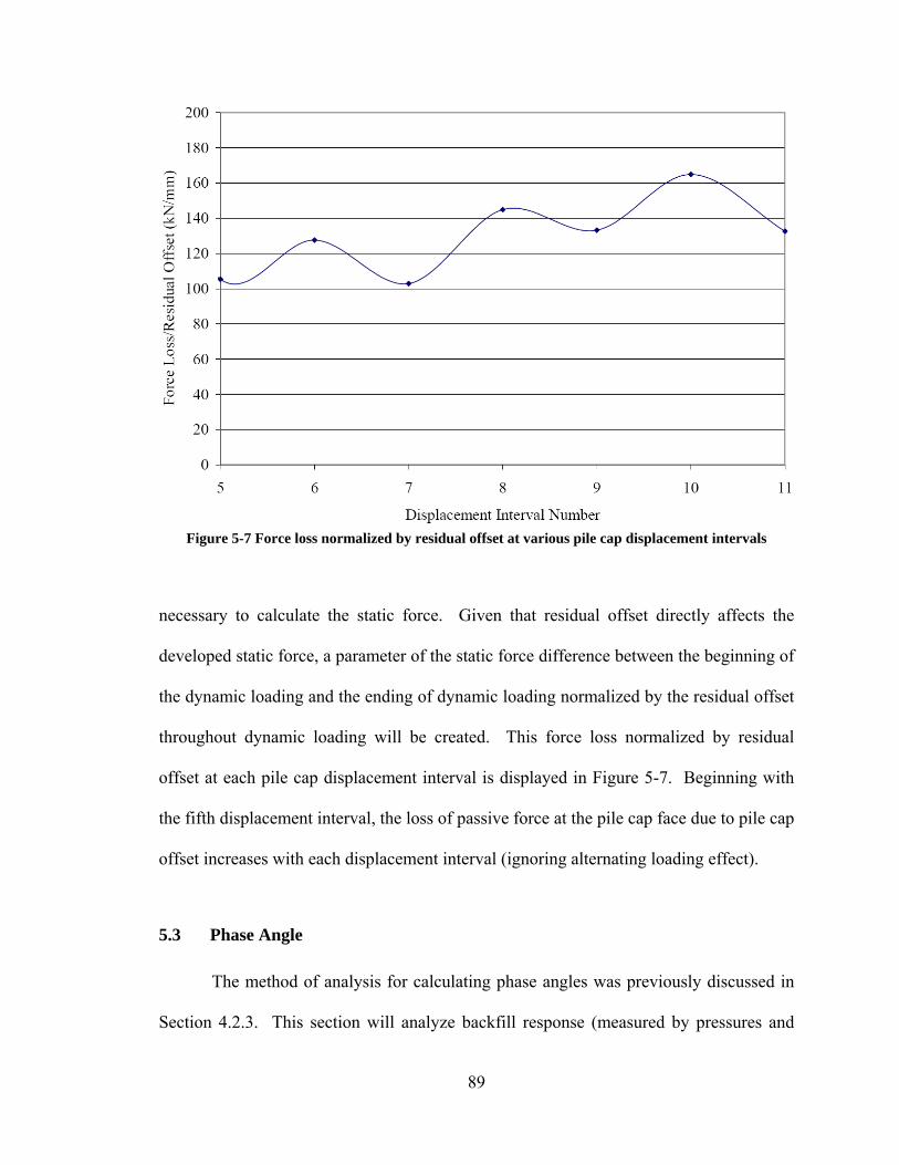
Figure 5-7 Force loss normalized by residual offset at various pile cap displacement intervals
necessary to calculate the static force. Given that residual offset directly affects the
developed static force, a parameter of the static force difference between the beginning of
the dynamic loading and the ending of dynamic loading normalized by the residual offset
throughout dynamic loading will be created. This force loss normalized by residual
offset at each pile cap displacement interval is displayed in Figure 5-7. Beginning with
the fifth displacement interval, the loss of passive force at the pile cap face due to pile cap
offset increases with each displacement interval (ignoring alternating loading effect).
5.3 Phase Angle
The method of analysis for calculating phase angles was previously discussed in
Section 4.2.3. This section will analyze backfill response (measured by pressures and
89

displacements) first through the depth of the backfill at the backfill-pile cap interface and
then at varying points across the backfill length.
5.3.1 Through the Depth of the Backfill
The pressure plate measurements during dynamic loading were presented in
Chapter 4.1.2. Figure 4-19 illustrated the pressures measured by each of the pressure
plates along the pile cap’s northern face. A closer look (a 1 second interval) at the
pressure plate measurements is displayed Figure 5-8 during Shake 8. This short interval
takes a snapshot of the changing pressures at mid-range forcing frequencies (about 6 Hz).
Generally, the pressures measured by each pressure plate rise and fall with similar
magnitudes and rate changes at similar time periods. This symmetry of motion suggests
Figure 5-8 Cap pressure time history at 100 seconds or 6 Hz, Shake 8
90
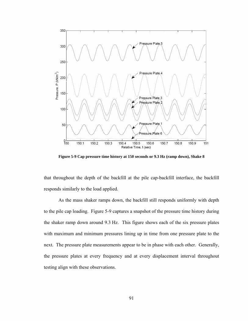
Figure 5-9 Cap pressure time history at 150 seconds or 9.3 Hz (ramp down), Shake 8
that throughout the depth of the backfill at the pile cap-backfill interface, the backfill
responds similarly to the load applied.
As the mass shaker ramps down, the backfill still responds uniformly with depth
to the pile cap loading. Figure 5-9 captures a snapshot of the pressure time history during
the shaker ramp down around 9.3 Hz. This figure shows each of the six pressure plates
with maximum and minimum pressures lining up in time from one pressure plate to the
next. The pressure plate measurements appear to be in phase with each other. Generally,
the pressure plates at every frequency and at every displacement interval throughout
testing align with these observations.
91

5.3.2 Across the Length of the Backfill
The relative movement of the pile cap and the backfill soil mass produce forces
on the pile cap face. This displacement-derived force can be treated as a spring.
However, the backfill mass itself is not a rigid nor elastic mass. Consequently, absolute
backfill displacement decreases with increasing distance from the moving pile cap face,
and even movement within the backfill mass may not be in phase at all points. As
explained previously, during cyclic loading backfill displacements can be reliably
measured by string potentiometers (whereas they cannot during dynamic loading due to
vibration effects on the reference frame).
5.3.2.1 Displacement during Cyclic Loading
Figure 5-10 and Figure 5-11, displaying displacements during Series 8 and Series
9, respectively, both show the pile cap moving approximately 0.7 mm forward and then
backward throughout cyclic loading. This motion was transferred through the soil where
displacement measurements were calculated at points located 0.61, 1.83, and 3.66 m
north of the pile cap face. While the displacement magnitudes at each backfill distance
vary, the peak displacements at various backfill positions generally align with the pile cap
peak displacements. The backfill appears to be generally in-phase with the pile cap. The
small irregularities at the beginning and ending of the time histories shown in the figures
are artifacts of the data filtering and integration process.
Another notable observation is the relationship of the soil displacements 3.66 m
and 1.83 m away from the pile cap. Intuition would say that the closer the soil is to the
pile cap the more impact the cap would have on the soil. However, the soil
displacements at 3.66 m are greater than those displacements at 1.83 m. One possible
92
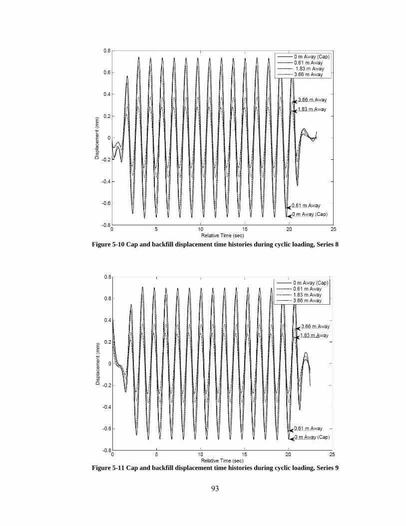
Figure 5-10 Cap and backfill displacement time histories during cyclic loading, Series 8
Figure 5-11 Cap and backfill displacement time histories during cyclic loading, Series 9
93
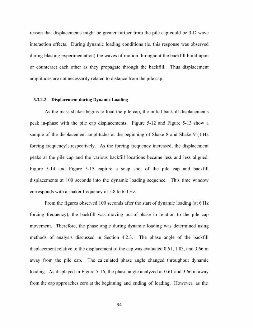
reason that displacements might be greater further from the pile cap could be 3-D wave
interaction effects. During dynamic loading conditions (ie. this response was observed
during blasting experimentation) the waves of motion throughout the backfill build upon
or counteract each other as they propagate through the backfill. Thus displacement
amplitudes are not necessarily related to distance from the pile cap.
5.3.2.2 Displacement during Dynamic Loading
As the mass shaker begins to load the pile cap, the initial backfill displacements
peak in-phase with the pile cap displacements. Figure 5-12 and Figure 5-13 show a
sample of the displacement amplitudes at the beginning of Shake 8 and Shake 9 (1 Hz
forcing frequency); respectively. As the forcing frequency increased, the displacement
peaks at the pile cap and the various backfill locations became less and less aligned.
Figure 5-14 and Figure 5-15 capture a snap shot of the pile cap and backfill
displacements at 100 seconds into the dynamic loading sequence. This time window
corresponds with a shaker frequency of 5.8 to 6.0 Hz.
From the figures observed 100 seconds after the start of dynamic loading (at 6 Hz
forcing frequency), the backfill was moving out-of-phase in relation to the pile cap
movement. Therefore, the phase angle during dynamic loading was determined using
methods of analysis discussed in Section 4.2.3. The phase angle of the backfill
displacement relative to the displacement of the cap was evaluated 0.61, 1.83, and 3.66 m
away from the pile cap. The calculated phase angle changed throughout dynamic
loading. As displayed in Figure 5-16, the phase angle analyzed at 0.61 and 3.66 m away
from the cap approaches zero at the beginning and ending of loading. However, as the
94
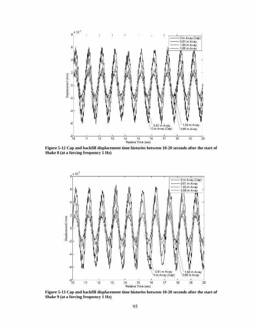
Figure 5-12 Cap and backfill displacement time histories between 10-20 seconds after the start of Shake 8 (at a forcing frequency 1 Hz)
Figure 5-13 Cap and backfill displacement time histories between 10-20 seconds after the start of Shake 9 (at a forcing frequency 1 Hz)
95

Figure 5-14 Cap and backfill displacement time histories 100 seconds after the start of Shake 8 (at a forcing frequency of 6 Hz)
Figure 5-15 Cap and backfill displacement time histories 100 seconds after the start of Shake 9 (at a forcing frequency of 6 Hz)
96
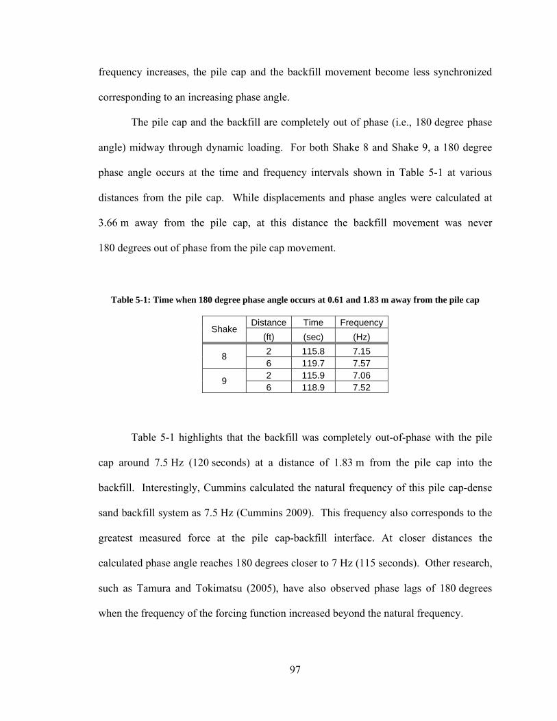
frequency increases, the pile cap and the backfill movement become less synchronized
corresponding to an increasing phase angle.
The pile cap and the backfill are completely out of phase (i.e., 180 degree phase
angle) midway through dynamic loading. For both Shake 8 and Shake 9, a 180 degree
phase angle occurs at the time and frequency intervals shown in Table 5-1 at various
distances from the pile cap. While displacements and phase angles were calculated at
3.66 m away from the pile cap, at this distance the backfill movement was never
180 degrees out of phase from the pile cap movement.
Table 5-1: Time when 180 degree phase angle occurs at 0.61 and 1.83 m away from the pile cap
Shake Distance Time Frequency
(ft) (sec) (Hz)
8 2 115.8 7.15 6 119.7 7.57
9 2 115.9 7.06 6 118.9 7.52
Table 5-1 highlights that the backfill was completely out-of-phase with the pile
cap around 7.5 Hz (120 seconds) at a distance of 1.83 m from the pile cap into the
backfill. Interestingly, Cummins calculated the natural frequency of this pile cap-dense
sand backfill system as 7.5 Hz (Cummins 2009). This frequency also corresponds to the
greatest measured force at the pile cap-backfill interface. At closer distances the
calculated phase angle reaches 180 degrees closer to 7 Hz (115 seconds). Other research,
such as Tamura and Tokimatsu (2005), have also observed phase lags of 180 degrees
when the frequency of the forcing function increased beyond the natural frequency.
97
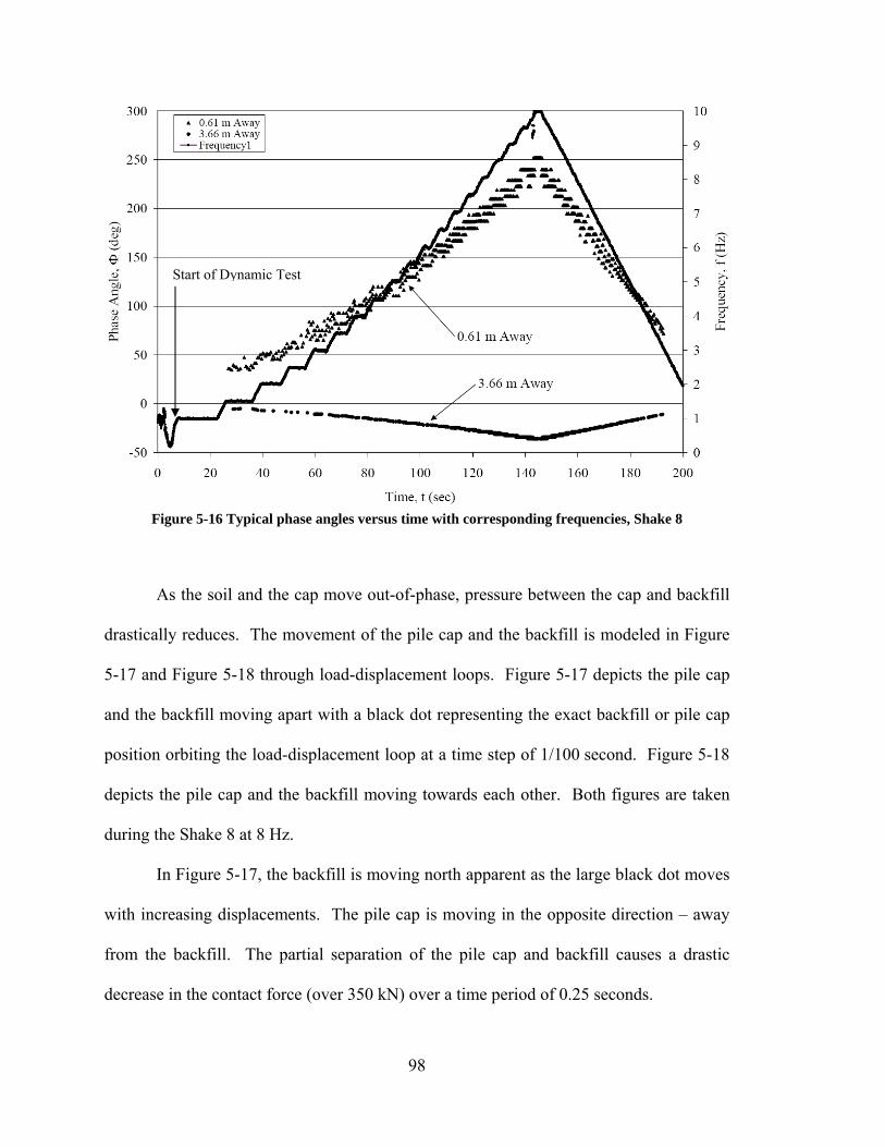
Start of Dynamic Test
Figure 5-16 Typical phase angles versus time with corresponding frequencies, Shake 8
As the soil and the cap move out-of-phase, pressure between the cap and backfill
drastically reduces. The movement of the pile cap and the backfill is modeled in Figure
5-17 and Figure 5-18 through load-displacement loops. Figure 5-17 depicts the pile cap
and the backfill moving apart with a black dot representing the exact backfill or pile cap
position orbiting the load-displacement loop at a time step of 1/100 second. Figure 5-18
depicts the pile cap and the backfill moving towards each other. Both figures are taken
during the Shake 8 at 8 Hz.
In Figure 5-17, the backfill is moving north apparent as the large black dot moves
with increasing displacements. The pile cap is moving in the opposite direction – away
from the backfill. The partial separation of the pile cap and backfill causes a drastic
decrease in the contact force (over 350 kN) over a time period of 0.25 seconds.
98
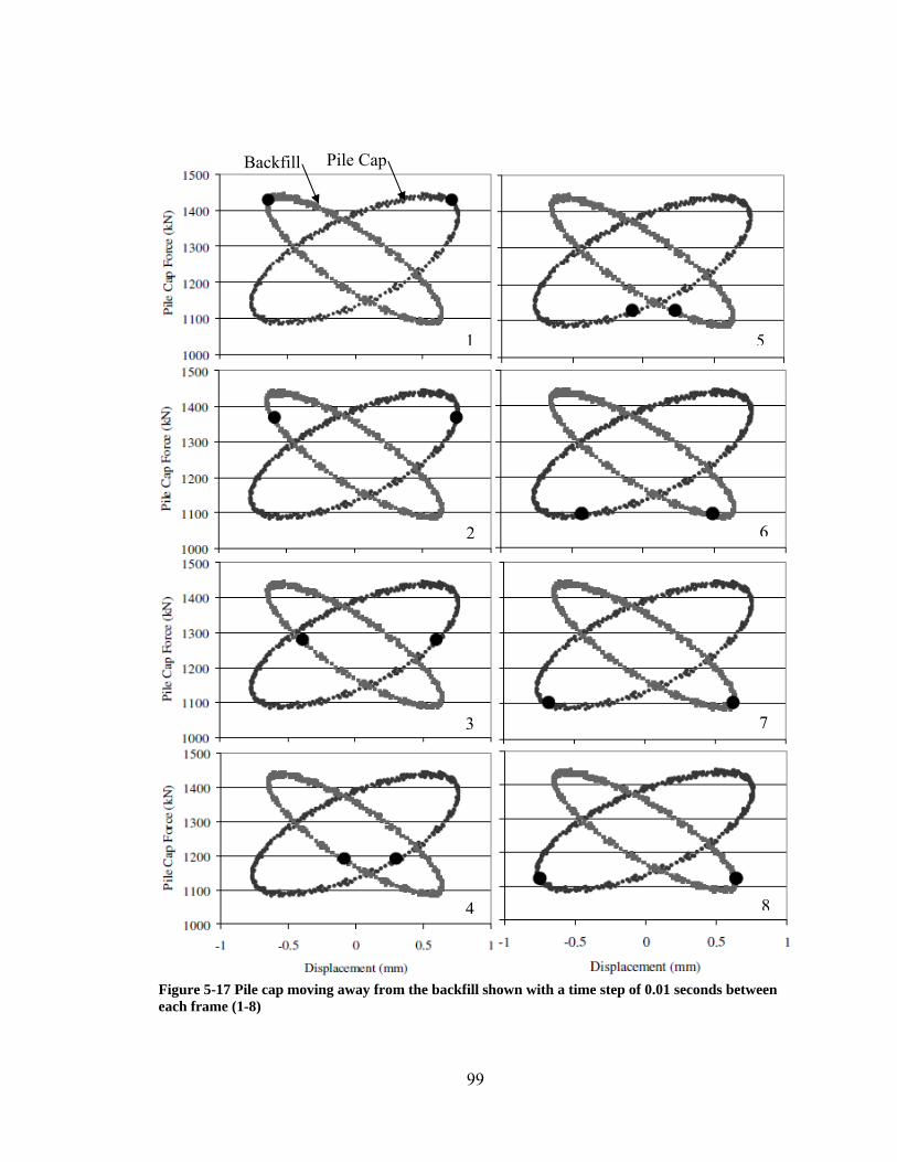
Pile Cap Backfill
1 5
62
73
84
Figure 5-17 Pile cap moving away from the backfill shown with a time step of 0.01 seconds between each frame (1-8)
99
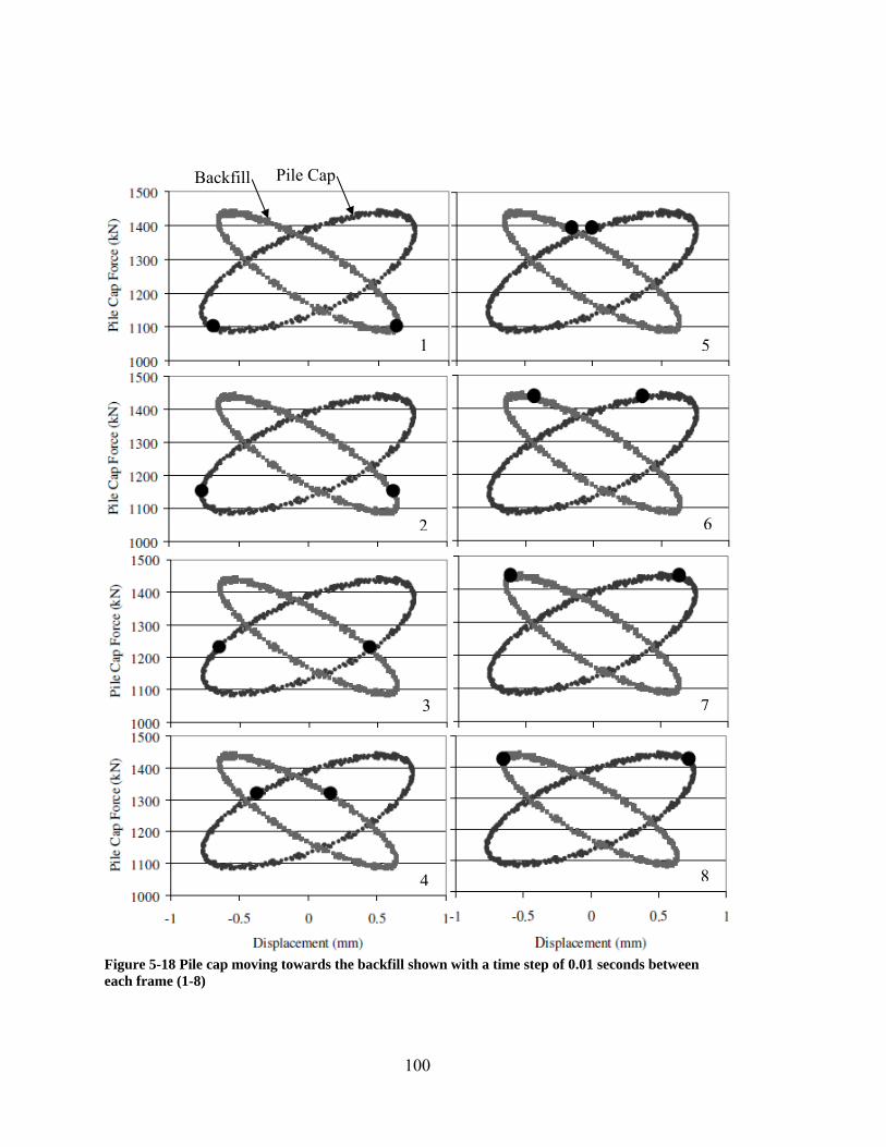
Pile Cap Backfill
1 5
62
73
84
Figure 5-18 Pile cap moving towards the backfill shown with a time step of 0.01 seconds between each frame (1-8)
100

Figure 5-18 shows the pile cap and the backfill moving towards each other. The
pile cap shifts from 0.8 mm south of its position at the beginning of the eighth
displacement interval to 0.8 mm north. The backfill moves from just over 0.6 mm north
to 0.6 mm south. The backfill does not move the full 0.8 mm that the pile cap displaces.
As these entities move closer, the contact force at the interface builds.
5.4 Damping
Calculations for assessing the damping of the system using load-displacement
loops were introduced in Section 4.2.4 (examples of load-displacement loops were
previously displayed in Figure 5-3 and Figure 5-4). Using the load-displacement loops
for the backfill, damping coefficients for the backfill were computed as a function of
forcing frequency. The results are shown in Figure 5-19, and it can be seen that the
damping coefficient is relatively constant with a value just larger than 3 kN-sec/mm.
101

0
1
2
3
4
5 6 7 8 9
Frequency, f (Hz)
Dam
ping
Coe
ffici
ent,
c (k
N*s
ec/m
m
10
)
Figure 5-19 Damping coefficient versus frequency, Shake 8
102
6 Interpretation of Results
The following chapter relies on the analyses contained in the previous chapters.
The contact force between the pile cap and the backfill will be examined to identify
changes in resistance due to cyclic and dynamic loadings. By isolating losses associated
with different mechanisms, the difference between the force under static loading
conditions and that under cyclic and dynamic loading conditions can be calculated. The
Mononobe-Okabe (M-O) equation is then used with a calibrated pseudo-static seismic
coefficient expressed as a faction of peak ground acceleration (PGA) as a means of
modeling or predicting cyclic and dynamic losses.
6.1 Identifying Components of Passive Contact Force
Force may be calculated from the simple relationship of stiffness and
displacement. A spring with a stiffness of 100 kN/m requires 100 kN to displace the
spring 1 m. If the spring was already compressed (i.e., being held in a displaced shape),
the initial force causing the compression plus the additional 100 kN to displace the spring
an extra meter may be added together to find the total static force. In a like manner, the
theoretical pile cap-backfill static contact force is equivalent to the relative displacement
amplitude of the pile cap from its initial position prior to the application of
cyclic/dynamic loads multiplied by the stiffness of the backfill and then adding the
103

actuator force initially used to displace the pile cap prior to the application of
cyclic/dynamic loads. This may be written as the following equation:
0FxkF amp +⋅= (6.1)
where:
F =theoretical static force at pile cap-backfill interface
k = backfill soil stiffness
xamp = pile cap displacement amplitude during dynamic loading
0F = initial static force at pile cap displacement interval
From this fundamental equation, a theoretical static force on the pile cap face is
calculated using the displacement amplitude of the pile cap and the measured static
stiffness of the backfill at that pile cap displacement interval.
6.1.1 Cyclic Effect
During cyclic loading, a linear increase in contact force was expected to occur
with pile cap displacement such that a higher displacement produces a higher force at the
pile cap-backfill interface. However, during cyclic loading, the contact force did not
increase as the pile cap displaced further into the backfill with each cycle. The force
losses may be attributed to cyclic effects. In other words, if no losses had occurred, the
same displacement amplitude should produce the same contact force. As seen in Figure
6-1(a), with repeated actuator cycling, less force is being mobilized with each cycle
104

despite similar displacement amplitudes. To quantify this force loss caused by cyclic
effects, another term was introduced into Equation 6.1. This term, as shown in Equation
6.2, is the product of the force loss per unit of residual offset (calculated in Equation 4.2)
and the trendline displacements (prepared in Section 4.1.1.2.2). The following equation
estimates contact force accounting for cyclic losses during dynamic loading:
0FxxF
xkF offset
Totaloffset
offsetamp +⋅⎟
⎟⎠
⎞⎜⎜⎝
⎛+⋅= (6.2)
where:
F = theoretical static force at pile cap-backfill interface
k = backfill soil stiffness
ampx = pile cap displacement amplitude
offsetF = force loss per unit of residual offset (a negative value)
offsetx = displacement trend during cyclic/dynamic loading
0F = initial static force at pile cap displacement interval
These parameters are shown during cyclic actuator loading conditions in Figure 6-1. In
Figure 6-1(a), the initial and peak forces are referenced, as is the displacement amplitude.
The displacement offset is the distance from the pile cap position corresponding with
peak force to the peak displacement during any given cycle. Foffset displays the observed
force loss associated with cyclic effects. Figure 6-1(b) and Figure 6-1(c) further
illustrate the relationship that as displacement offset increases, force offset decreases.
105
Since force loss during the dynamic shaker loading is in part due to similar cyclic effects,
Equation 6.2 can also be used to reasonably approximate cyclic losses during the
dynamic shaker loading and thus approximately separate losses due to cyclic loading and
losses due to other dynamic mechanisms such as out-of-phase movement of the cap and
backfill. The equivalent parameters for Equation 6.2 during dynamic shaker loading are
shown in Figure 6-2.
When applied throughout Shake 8 and Shake 10 (displacement intervals which
were loaded dynamically first and where passive force appears to have been nearly or
fully mobilized along the failure plane), Equation 6.2 produces the results displayed in
Figure 6-3 and Figure 6-4, respectively. The contact force at the beginning of Shake 8 is
approximately 1425 kN, and at the start of Shake 10 the initial force just above 1600 kN.
At the scale shown, individual loading cycles cannot be distinguished by the maximum
and minimum forces during each cycle which bound the shaded area formed by all of the
load cycles. The force peaks around 7.5 Hz or 118 seconds into Shake 8. Shake 10 also
reaches maximum force at 7.5 Hz. Afterward, the contact force decreases as the shaker
frequency (and force) continue to ramp up. As the ramp-down of the eccentric mass
shaker begins, the maximum and minimum forces during each load cycle begin to
converge as the dynamic amplitude decreases, reaching an ending static force of 1092 kN
for Shake 8 and 1266 kN for Shake 10.
Both Figure 6-3 and Figure 6-4 display the force decrease due to cyclic effects.
The total residual offset in Shake 8 was 2.32 mm which accounted for over 333 kN of
total force loss from the beginning to the end of the dynamic loading. During Shake 10,
the residual offset was measured at 2.07 mm resulting in 341 kN of total force loss.
106

(a)
(b)
(c)
Figure 6-1 Depiction of force and displacement parameters during cyclic loading
107
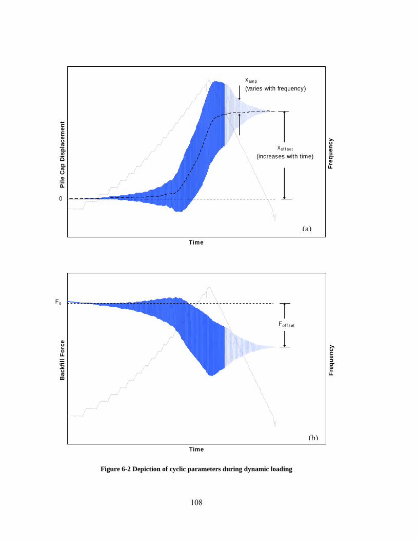
Time
Pile
Cap
Dis
plac
emen
t
Freq
uenc
y
xof f set
(increases with time)
xamp
(varies with frequency)
0
(a)
Time
Back
fill F
orce
Freq
uenc
yFof f set
Fo
(b)
Figure 6-2 Depiction of cyclic parameters during dynamic loading
108
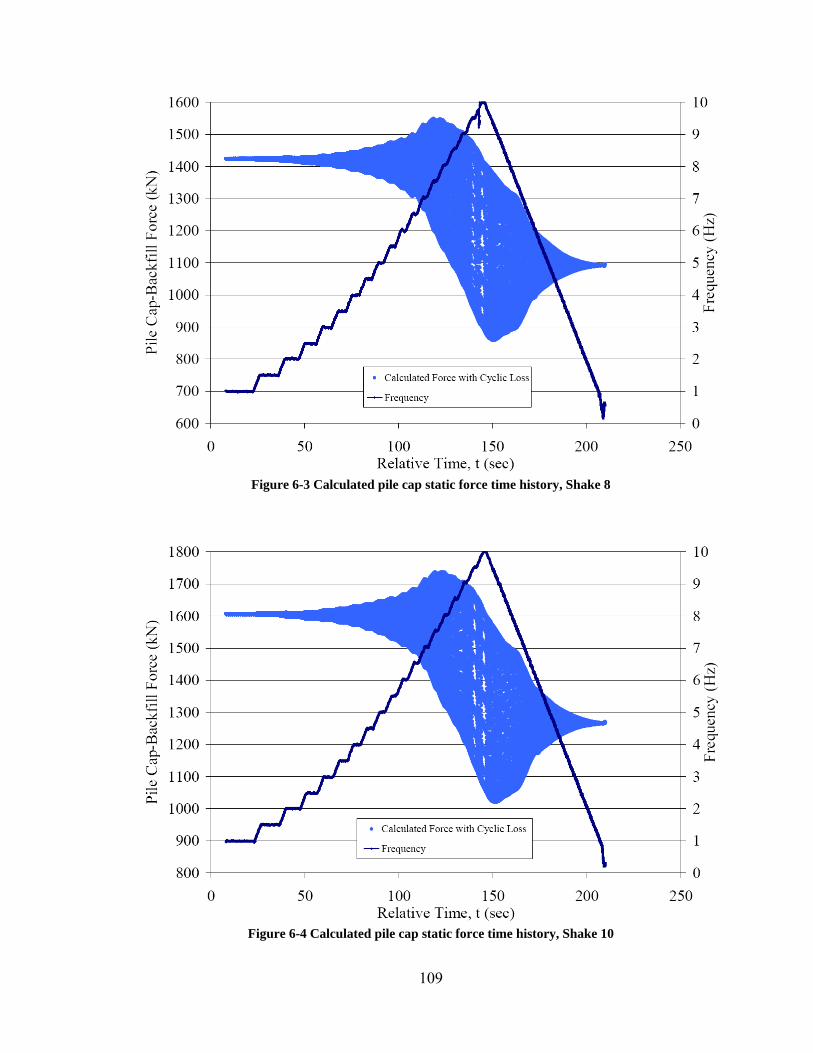
Figure 6-3 Calculated pile cap static force time history, Shake 8
Figure 6-4 Calculated pile cap static force time history, Shake 10
109
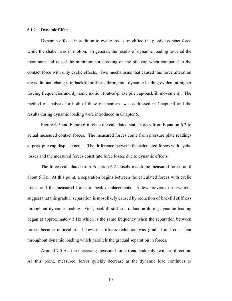
6.1.2 Dynamic Effect
Dynamic effects, in addition to cyclic losses, modified the passive contact force
while the shaker was in motion. In general, the results of dynamic loading lowered the
maximum and raised the minimum force acting on the pile cap when compared to the
contact force with only cyclic effects. Two mechanisms that caused this force alteration
are additional changes in backfill stiffness throughout dynamic loading evident at higher
forcing frequencies and dynamic motion (out-of-phase pile cap-backfill movement). The
method of analysis for both of these mechanisms was addressed in Chapter 4 and the
results during dynamic loading were introduced in Chapter 5.
Figure 6-5 and Figure 6-6 relate the calculated static forces from Equation 6.2 to
actual measured contact forces. The measured forces come from pressure plate readings
at peak pile cap displacements. The difference between the calculated forces with cyclic
losses and the measured forces constitute force losses due to dynamic effects.
The forces calculated from Equation 6.2 closely match the measured forces until
about 5 Hz. At this point, a separation begins between the calculated forces with cyclic
losses and the measured forces at peak displacements. A few previous observations
suggest that this gradual separation is most likely caused by reduction of backfill stiffness
throughout dynamic loading. First, backfill stiffness reduction during dynamic loading
began at approximately 5 Hz which is the same frequency when the separation between
forces became noticeable. Likewise, stiffness reduction was gradual and consistent
throughout dynamic loading which parallels the gradual separation in forces.
Around 7.5 Hz, the increasing measured force trend suddenly switches direction.
At this point, measured forces quickly decrease as the dynamic load continues to
110
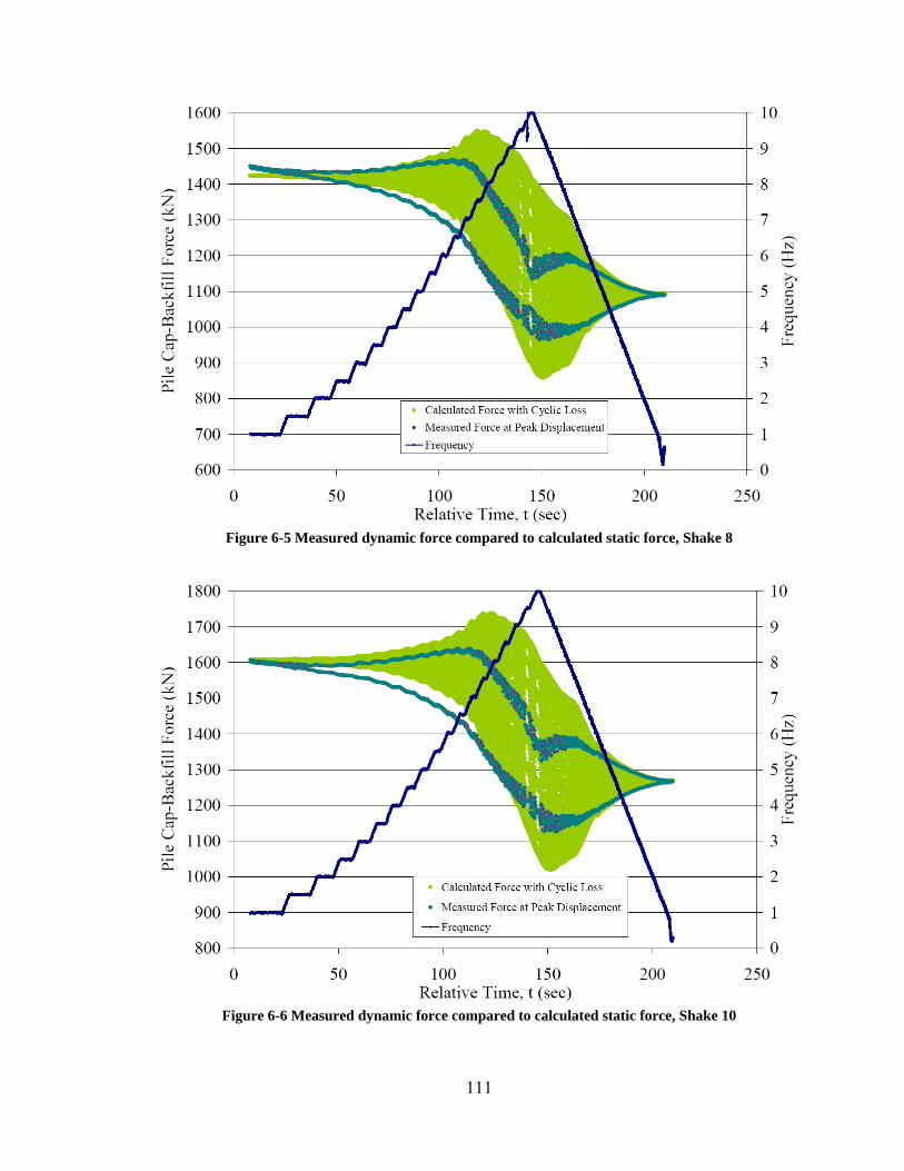
Figure 6-5 Measured dynamic force compared to calculated static force, Shake 8
Figure 6-6 Measured dynamic force compared to calculated static force, Shake 10
111

ramp-up. This sudden shift in the development of passive contact force may be attributed
to the dynamic effects of phase lag. Similar effects have been noted by Tokimatsu et al.
(2004) in their study of large shaking table tests involving piled foundations. During
cyclic loading there was a steady increase and decrease in force which matched the
movement of the pile cap into the soil suggesting that the backfill was in-phase with the
pile cap. At the beginning of dynamic loading, contact force developed similarly to
cyclic conditions. Likewise, the pile cap and the soil were generally in-phase. However,
during dynamic loading as the forcing frequency of the mass shaker increased, the soil
movement began to lag behind the pile cap movement. When the frequency approached
7.5 Hz, the soil was almost completely out-of-phase with the pile cap. This is the same
point that the measured contact force drastically and unexpectedly declines contrary to
the calculated force with cyclic losses. As the frequency continues to ramp-up to 10 Hz
the separation between the calculated force and actual force widens.
6.1.3 Damping Effect
Damping, another dynamic effect, counteracts a portion of the contact force losses
outlined above. Damping, as computed in Section 5.4, increases the passive contact force
acting on the pile cap face. This increase is proportional to the increase in frequency (as
previously described and depicted as load-displacement loops widen). At greater
frequencies, the maximum force separates from the force at maximum displacement
(shown in Figure 4-25). The difference between the maximum measured force and the
force at maximum displacement is force gain due to damping.
112
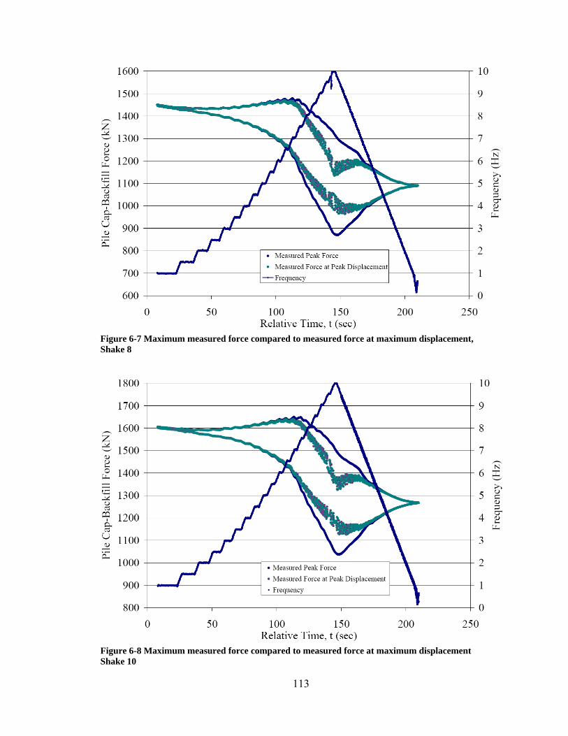
Figure 6-7 Maximum measured force compared to measured force at maximum displacement, Shake 8
Figure 6-8 Maximum measured force compared to measured force at maximum displacement Shake 10
113

Figure 6-7 and Figure 6-8 show the maximum measured force and the measured
force at maximum displacement for Shake 8 and Shake 10, respectively. Notice that at
10 Hz, approximately 150 seconds, the damping effect (the difference between the two
force distributions) is the greatest. This aligns with the damping calculations from load-
displacement loops discussed in Section 5.4. Damping is seemingly insignificant at
below 7 Hz during both dynamic loading sequences.
6.1.4 Passive Force Loading Comparison
To further illustrate the changes in the pile cap force during dynamic loading,
Figure 6-9 and Figure 6-10 overlay the various measured and computed forces. The
theoretical static force was first calculated from Equation 6.1. Adding residual offset
parameters (Equation 6.2) adjusted this static force to a reasonable estimate of the force
including cyclic losses during dynamic loading. The resulting force is referred to as the
boundary line because it distinguishes between the losses attributable to cyclic effects
(like those observable during the cyclic actuator loading cycles, represented in the figures
by Arrow A) and dynamic effects (like those observed during dynamic shaker loading
cycles, above and beyond any cyclic effects, represented in the figures by Arrow B). The
force measured by pressure plates at maximum displacement represents the static force
minus all cyclic and dynamic losses. Also shown in the figures is a line representing the
peak measured force measured by pressure plates. This force includes the added
damping force; the magnitude of the damping force is represented by Arrow C.
114
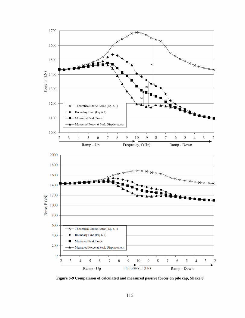
3 4 5 6 7 8 9 10 9 8 6 7 5 4 32
Ramp - Down Ramp - Up
2
3 4 5 6 7 8 9 10 9 8 6 7 5 4 3
Ramp - Down Ramp - Up
2 2
Figure 6-9 Comparison of calculated and measured passive forces on pile cap, Shake 8
115

8 6 56 102 93 4 5 3 7 8 7 4 29
Ramp - Up Ramp - Down
Ramp - Down Ramp - Up
Figure 6-10 Comparison of calculated and measured passive forces on pile cap, Shake 10
116

For both Shake 8 and Shake 10, the effects of damping at 10 Hz raise the force
approximately 10%. The figures for Shake 8 and Shake 10 are quite similar, suggesting a
consistency in effects once passive earth forces are nearly or fully mobilized.
6.2 Mononobe-Okabe
The Mononobe-Okabe (M-O) equation is probably the most widely used method
to determine the dynamic effects of active and passive earth pressures on a structure.
Inherent to this equation are several assumptions which must be satisfied. Some of these
assumptions were generally satisfied throughout the entire testing (i.e., homogenous,
cohesionless backfill was used for testing). However, other M-O assumptions were only
satisfied at certain points during testing. For example, the M-O equation is dependent on
fully mobilizing the shear strength of the backfill which occurred after the eighth pile cap
displacement interval.
The M-O equation does not explicitly account for dynamic losses due to soil
stiffness reduction, phase lag, or damping. Phase lag became apparent when the
frequency of the mass shaker increased and the pile cap and the backfill began to move
comparatively out-of-phase. The M-O equation is a pseudo-static (or perhaps more
correctly a pseudo-dynamic) equation based on static equilibrium relationships and hence
does not explicitly account for damping effects which are variable with dynamic loading
frequency. While the M-O equation does not explicitly account for non-integral
movement between the backfill and retaining structure, backfill stiffness reduction, or
damping, the M-O equation computes the lowest passive earth force between the backfill
117
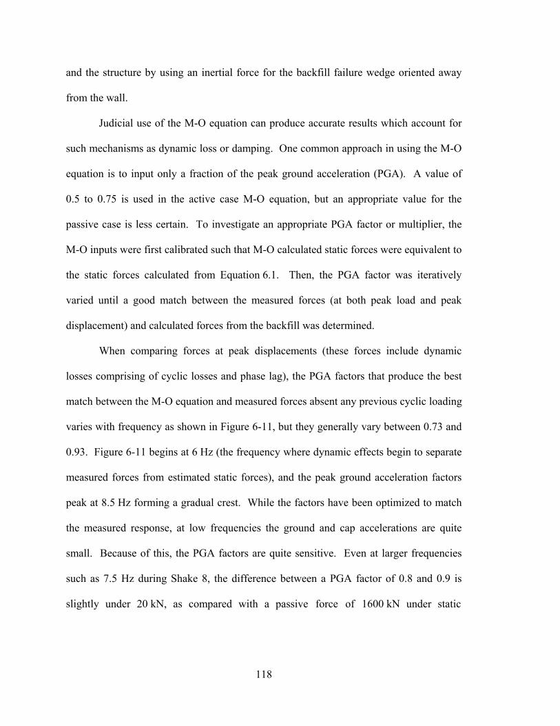
and the structure by using an inertial force for the backfill failure wedge oriented away
from the wall.
Judicial use of the M-O equation can produce accurate results which account for
such mechanisms as dynamic loss or damping. One common approach in using the M-O
equation is to input only a fraction of the peak ground acceleration (PGA). A value of
0.5 to 0.75 is used in the active case M-O equation, but an appropriate value for the
passive case is less certain. To investigate an appropriate PGA factor or multiplier, the
M-O inputs were first calibrated such that M-O calculated static forces were equivalent to
the static forces calculated from Equation 6.1. Then, the PGA factor was iteratively
varied until a good match between the measured forces (at both peak load and peak
displacement) and calculated forces from the backfill was determined.
When comparing forces at peak displacements (these forces include dynamic
losses comprising of cyclic losses and phase lag), the PGA factors that produce the best
match between the M-O equation and measured forces absent any previous cyclic loading
varies with frequency as shown in Figure 6-11, but they generally vary between 0.73 and
0.93. Figure 6-11 begins at 6 Hz (the frequency where dynamic effects begin to separate
measured forces from estimated static forces), and the peak ground acceleration factors
peak at 8.5 Hz forming a gradual crest. While the factors have been optimized to match
the measured response, at low frequencies the ground and cap accelerations are quite
small. Because of this, the PGA factors are quite sensitive. Even at larger frequencies
such as 7.5 Hz during Shake 8, the difference between a PGA factor of 0.8 and 0.9 is
slightly under 20 kN, as compared with a passive force of 1600 kN under static
118

Figure 6-11 PGA factor applied to M-O equation to account for dynamic losses, Shake 8
Measured Peak Force
Figure 6-12 Force produced by the M-O equation with various PGA factors, Shake 8
119

conditions. As shown in Figure 6-12, a PGA factor of 0.84 at 6 Hz provides the best
match. A factor of 0.75 to 0.9 appears to consistently provide the best overall match.
The maximum PGA used in this analysis was 0.43 g, occurring at a shaker frequency of
10 Hz, while the PGA at 7.5 Hz was 0.16 g.
PGA factors for Shake 10 are displayed in Figure 6-13 for comparison purposes.
At lower frequencies, the factor which produces the best match with measured force is
somewhat higher than those observed in Shake 8. At higher frequencies (6.5 Hz and
above), the PGA factor that produces the closest overall match to measured force is 0.8.
These values are generally similar to factors produced in Shake 8. Figure 6-14 compares
the measured force with forces computed using the M-O equation at various PGA factors,
with values of about 0.75 providing the best match. At lower frequencies, a large
difference between PGA factors does not significantly change the calculated force, as
was observed previously in the data from Shake 8.
Including increases in resisting force due to damping will reduce the total
dynamic losses. Therefore, the PGA factor which will model dynamic loading conditions
including the effects of damping should be less than those presented above. Figure 6-15
and Figure 6-17 display the PGA factors which provide the best match to peak force for
Shake 8 and Shake 10, respectively. The PGA factor generally ranges between 0.55 and
0.7 at higher forcing frequencies. The corresponding forces that are calculated by various
PGA factors including the effects of damping are shown in Figure 6-16 and Figure 6-18
for Shake 8 and Shake 9, respectively. Generally, it appears that the M-O equation may
be used to calculate the dynamic passive earth forces considering damping by applying a
0.55 to 0.65 multiplier to the PGA.
120

Figure 6-13 PGA factor applied to M-O equation to account for dynamic losses, Shake 10
Measured Peak Force
Figure 6-14 Force produced by the M-O equation with various PGA factors, Shake 10
121

Figure 6-15 PGA factor applied to M-O equation to account for dynamic losses with damping, Shake 8
Measured Peak Force
Figure 6-16 Force including damping effects produced by the M-O equation with various PGA factors, Shake 8
122
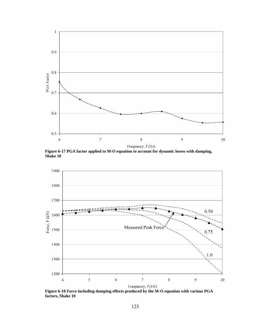
Figure 6-17 PGA factor applied to M-O equation to account for dynamic losses with damping, Shake 10
Measured Peak Force
Figure 6-18 Force including damping effects produced by the M-O equation with various PGA factors, Shake 10
123

124

7 Conclusion
This thesis analyzed data derived from full scale testing of a pile cap system with
a densely compacted sand backfill under static, cyclic, and dynamic loadings. This data
was collected on site on May 25, 2007 as part of a larger series of testing. Particular
focus has been placed on interpretation of the passive behavior of the backfill based on
the soil pressures measured directly by the pressure plates. Based on this work, the
following observations, conclusions, and recommendations are presented.
1. Passive earth force develops as the cap is pushed into the backfill. Under
slow, cyclic loading, the observed backfill stiffness is relatively constant.
Under faster, dynamic loading, the observed backfill stiffness decreases in a
relatively linear fashion (with an observed rate of 50 kN/mm for every 1 Hz
increase in forcing frequency above 5 Hz).
2. During cyclic and dynamic loading, the pile cap gradually develops a residual
offset from its initial position. This offset is accompanied by a reduction in
contact force from the backfill. Backfill which had previously experienced
cyclic loading at similar displacements exhibited considerably smaller offsets
during dynamic loading because of previous loading effects.
3. The pile cap and the backfill appeared to move integrally during static and
cyclic loadings. However, during dynamic loading, the backfill exhibited
125
some out-of-phase movement relative to the pile cap. At 7.5 Hz (the natural
frequency of the pile cap-backfill system) the backfill and the pile cap reached
a phase angle of 180 degrees suggesting complete out-of-phase movement.
4. Observed losses in contact force were associated with both cyclic (softening
due to repeated loading) and dynamic (out-of-phase movement) effects. Force
losses due to dynamic loading increased with increasing frequency (which
corresponded to larger displacements)
5. Losses due to dynamic loading were offset somewhat by increases in peak
force due to damping. Damping effects shift the occurrence of peak force at
the pile cap-backfill interface to a point before peak pile cap displacements are
reached. The increase in contact force due to damping was observed to be
relatively proportional to increasing frequency.
6. Passive earth forces with cyclic/dynamic losses without considering damping
can be reasonably estimated using the Mononobe-Okabe (M-O) equation with
a 0.75 or 0.8 multiplier applied to the peak ground acceleration (PGA). More
specifically, these multipliers ranged between 0.70 and 0.93 during dynamic
loadings from 6 Hz to 10 Hz.
7. Passive earth forces with cyclic/dynamic losses including the effect of backfill
damping can be reasonably estimated using the Mononobe-Okabe (M-O)
equation with a 0.6 multiplier applied to the peak ground acceleration (PGA).
126

References
Brinch Hansen, J. (1996). “Resistance of a rectangular anchor slab.” Bulletin No. 21. Danish Geotechnical Institute, Copenhagen, 12-13.
Caltrans (2001). “Seismic design criteria version 1.2.” California Department of Transportation, Sacramento, California.
Chandrasekaran, S. S. (2009). “Behaviour of pile groups under static, cyclic and dynamic lateral loading in clay.” PhD Dissertation, Dept. of Civil Engineering, Indian Institute of Technology Madras, Chennai, India.
Christensen, D. S. (2006). “Full scale static lateral load test of a 9 pile group in sand.” MS Thesis, Dept. of Civil and Environmental Engineering, Brigham Young University, Provo, Utah.
Chopra, A. K. (2001). Dynamics of structures. Upper Saddle River, Prentice Hall, New Jersey.
Cole, R. T. (2003). “Full-scale effects of passive earth pressure on the lateral resistance of pile caps.” PhD Dissertation, Brigham Young University, Provo, Utah.
Cole, R. T. and Rollins, K. M. (2006). “Passive earth pressure mobilization during cyclic loading.” Journal of Geotechnical and Geoenvironmental Engineering, ASCE, 132(9), 1154-1164.
Cummins, C. R. (2009). “Behavior of a full-scale pile cap with loosely and densely compacted clean sand backfill under cyclic and dynamic loadings.” MS Thesis, Dept. of Civil and Environmental Engineering, Brigham Young University, Provo, Utah.
Douglas, D. J. and Davis, E. H. (1964). “The movements of buried footings due to moment and horizontal load and the movement of anchor plates.” Geotechnique, London, 14(2), 115–132.
Duncan, J. M. and Mokwa, R. L. (2001). “Passive earth pressures: theories and tests.” Journal of. Geotechnical and Geoenvironmental Engineering, ASCE, 127(3), 248-257
127
Geokon (2004). “Model 3500/3510 earth pressure cells.” Instruction Manual, Geokon Inc.
Jacobsen, L. S. (1939). Described in Appendix D of “The Kentucky Project.” Technical Report No. 13, Tennessee Valley Authority, 1951.
Kramer, S. L. (1996). Geotechnical earthquake engineering. Upper Saddle River, Prentice Hall, New Jersey.
Matsuo, H. (1941). “Experimental study on the distribution of earth pressure acting on a vertical wall during earthquakes.” Journal of the Japan Society of Civil Engineers Japanese Society of Civil Engineers 27(2).
Mononobe, N. and Matsuo, H. (1929). “On the determination of earth pressures during earthquakes.” Proceeding, World Engineering Congress.
NCHRP (2008). “Seismic analysis and design of retaining walls, buried structures, slopes and embankments.” Report 661, National Cooperative Highway Research Program, 69-76.
Okabe, S. (1926). “General theory of earth pressures.” Journal of the Japan Society of Civil Engineers, Japanese Society of Civil Engineers 12(1).
Ostadan, F. and White, W. H. (1997). “Lateral seismic soil pressure – an updated approach.” US-Japanese SSI Workshop, Bechtel Corporation, San Francisco, California.
Ovesen, N. K. (1964). “Anchor slabs, calculation methods, and model tests.” Bulletin No. 16, Danish Geotechnical Institute, Copenhagen, 5-39.
Peterson, K. T. (1996). “Static and dynamic lateral load testing a full-scale pile group in clay.” MS Thesis, Dept. of Civil and Environmental Engineering, Brigham Young University, Provo, Utah.
Richards, R. J. and Elms, D. G. (1979). “Seismic behavior of gravity retaining walls.” Journal of the Geotechnical Engineering Division, ASCE, 449-465.
Rollins, K. M., King, R., Snyder, J. E., and Johnson, S. R. (2005a). “Full-scale lateral load tests of pile groups and drilled shafts in clay.” Procs. Intl. Conf. on Soil-Structure Interaction, Calculation Methods and Engineering Practice, Vol. 1, Ulitsky, V. M., Ed., ASV Publishers, Moscow: 287-292.
Rollins, K. M., Snyder, J. L., and Broderick, R. D. (2005b) “Static and dynamic response of a 15 pile group.” Proceedings 16th Intl. Conf. on Soil Mechanics and Geotechnical Engineering, Rotterdam, Netherlands, 2035-2040.
128
Runnels, I. K. (2007). “Cyclic and dynamic full-scale testing of a pile cap with loose silty sand backfill.” MS Thesis, Dept. of Civil and Environmental Engineering, Brigham Young University, Provo, Utah.
Seed, H. B. and Whitman, R. V. (1970). “Design of earth retaining structures for dynamic loads.” 1970 Specialty Conference, Cornell University, Ithaca, New York.
Tamura, S. and Tokimatsu, K. (2005). “Seismic earth pressure acting on embedded footing based on large-scale shaking table tests.” Seismic Performance and Simulation of Pile Foundations in Liquefied and Laterally Spreading Ground (GSP 145), ASCE, Davis, California.
Taylor, A. J. (2006). “Full-scale-lateral-load test of a 1.2 m diameter drilled shaft in sand.” MS Thesis, Dept. of Civil and Environmental Engineering, Brigham Young University, Provo, Utah.
Tokimatsu, K., Suzuki, H., and Sato, M. (2004). "Influence of initial and kinematic components on pile response during earthquakes." Procs. 11th Intl. Conf. on Soil Dynamics and Earthquake Engineering and 3rd Intl. Conf. on Earthquake Geotechnical Engineering. University of California, Berkeley. Doolin, D., Kammerer, A., Nogami, T., Seed, R. B., and Towhata, I., Eds. Vol. 1, 768-775.
U.S. Navy. (1986). Foundations and Earth Structures - Design Manual 7.2. Navy Facilities Engineering Command, Alexandria, Va.
Valentine, T. J. (2007). “Dynamic testing of a full-scale pile cap with dense silty sand backfill.” MS Thesis, Dept. of Civil and Environmental Engineering, Brigham Young University, Provo, Utah.
Whitman, R. V. (1990). “Seismic design and behavior of gravity retaining walls.” Geotechnical Special Publication 25, Design and Performance of Earth Retaining Structures, ASCE, 817-842.
129

130