partitioning perfect graphs into stars
TRANSCRIPT
HAL Id: hal-01494420https://hal.archives-ouvertes.fr/hal-01494420
Submitted on 23 Mar 2017
HAL is a multi-disciplinary open accessarchive for the deposit and dissemination of sci-entific research documents, whether they are pub-lished or not. The documents may come fromteaching and research institutions in France orabroad, or from public or private research centers.
L’archive ouverte pluridisciplinaire HAL, estdestinée au dépôt et à la diffusion de documentsscientifiques de niveau recherche, publiés ou non,émanant des établissements d’enseignement et derecherche français ou étrangers, des laboratoirespublics ou privés.
Partitioning Perfect Graphs into StarsRené van Bevern, Robert Bredereck, Laurent Bulteau, Jiehua Chen, Vincent
Froese, Rolf Niedermeier, Gerhard J. Woeginger
To cite this version:René van Bevern, Robert Bredereck, Laurent Bulteau, Jiehua Chen, Vincent Froese, et al.. Par-titioning Perfect Graphs into Stars. Journal of Graph Theory, Wiley, 2017, 85 (2), pp.297-335.�10.1002/jgt.22062�. �hal-01494420�

Partitioning Perfect Graphs into Stars∗
Rene van Bevern1,2, Robert Bredereck2, Laurent Bulteau3, Jiehua Chen2,Vincent Froese2, Rolf Niedermeier2, and Gerhard J. Woeginger4
1Novosibirsk State University, Novosibirsk, Russian Federation, [email protected] fur Softwaretechnik und Theoretische Informatik, TU Berlin, Germany,
{robert.bredereck,jiehua.chen,vincent.froese,rolf.niedermeier}@tu-berlin.de3Institut Gaspard-Monge, Universite Paris-Est Marne-la-Vallee, France
[email protected] of Mathematics and Computer Science, TU Eindhoven, The Netherlands,
March 23, 2017
Abstract
The partition of graphs into “nice” subgraphs is a central algorithmicproblem with strong ties to matching theory. We study the partitioningof undirected graphs into same-size stars, a problem known to be NP-complete even for the case of stars on three vertices. We perform athorough computational complexity study of the problem on subclassesof perfect graphs and identify several polynomial-time solvable cases, forexample, on interval graphs and bipartite permutation graphs, and alsoNP-complete cases, for example, on grid graphs and chordal graphs.
1 Introduction
We study the computational complexity (tractable versus intractable cases) ofthe following basic graph problem.
Star PartitionInput: An undirected n-vertex graph G = (V,E) and an integer s ∈ N.Question: Can the vertex set V be partitioned into k := dn/(s + 1)e mutu-
ally disjoint vertex subsets V1, V2, . . . , Vk, such that each subgraph G[Vi]contains an s-star (a K1,s)?
Two prominent special cases of Star Partition are the case s = 1 (findinga perfect matching) and the case s = 2 (finding a partition into connected
∗An extended abstract of this work appeared under the title “Star Partitions of PerfectGraphs” in Proceedings of the 41st International Colloquium on Automata, Languages, andProgramming (ICALP’14), Part I, LNCS 8572, pp. 174–185, Springer, 2014.
1

NP-complete
P
perfect
chordal
splitinterval
unitinterval
comparability
permutation
cograph
triviallyperfect
threshold(P3 known [33])
bipartite [7]
chordalbipartite
bipartitepermutation
subcubic planarbipartite [22, 23]
subcubicgrid
series-parallel [31]
tree
Figure 1: Complexity classification of Star Partition. Bold borders indicateresults of this paper. An arrow from a class A to a class B indicates thatA contains B. In most classes, NP-completeness results hold for s = 2 (that is,for P3-Partition). However, on split graphs, Star Partition is polynomi-al-time solvable for s ≤ 2, while it is NP-complete for s ≥ 3. P3-Partition issolvable on interval graphs in quasilinear time. We are not aware of any resultfor permutation graphs, chordal bipartite graphs, interval graphs (for s ≥ 3), orgrid graphs (for s = 3).
triples). Perfect matchings (s = 1), of course, can be found in polynomial time.Partitions into connected triples (the case s = 2), however, are hard to find; thisproblem, denoted P3-Partition, was proven to be NP-complete by Kirkpatrickand Hell [18].
Our goal in this paper is to achieve a better understanding of star partitionsfor certain subclasses of perfect graphs. We provide a fairly complete classificationin terms of polynomial-time solvability versus NP-completeness on the mostprominent subclasses of perfect graphs, leaving a few potentially challengingcases open; see Figure 1 for an overview of our results.
Motivation. The literature in algorithmic graph theory is full of packingand partitioning problems (packing is an optimization variant of partitioning,where one tries to maximize the number of disjoint vertex subsets). Concerningpractical relevance, note that P3-Packing and P3-Partition find applicationsin dividing distributed systems into subsystems [20] as well as in the TestCover problem arising in bioinformatics [13]. In particular, the applicationin distributed systems explicitly motivates the consideration of very restricted(perfect) graph classes such as grid-like structures. Star Partition on grid
2
graphs naturally occurs in political redistricting problems [4]. We show thatStar Partition remains NP-hard on subcubic grid graphs.
Interval graphs are a further famous class of perfect graphs. Here, StarPartition can be considered a team formation problem: Assume that we havea number of agents, each being active during a certain time interval. Our goal isto form teams, all of the same size, such that each team contains at least oneagent sharing time with every other team member. This specific team memberbecomes the team leader, since he or she can act as an information hub. Formingsuch teams is nothing else than solving Star Partition on interval graphs. Wepresent efficient algorithms for Star Partition on unit interval graphs (thatis, for the case when all agents are active for the same amount of time) and forP3-Partition on general interval graphs.
Related work. Packing and partitioning problems are central problems in algo-rithmic graph theory with many applications and with close connections to match-ing theory [35]. In the case of packing, one wants to maximize the number of graphvertices that are “covered” by vertex-disjoint copies of some fixed pattern graphH.In the case of partitioning, one wants to cover all vertices in the graph. We focuson the partitioning problem, which is also called H-Factor in the literature. Inthis work, we always refer to it as H-Partition. Since Kirkpatrick and Hell [18]established the NP-completeness of H-Partition on general graphs for every con-nected pattern H with at least three vertices, one branch of research has turnedto the investigation of classes of specially structured graphs. For instance, on theupside, H-Partition has been shown to be polynomial-time solvable on treesand series-parallel graphs [31] and on graphs of maximum degree two [23]. On thedownside, Pk-Partition (for each fixed k ≥ 3) remains NP-complete on planarbipartite graphs [14]; this hardness result is generalized to H-Partition on pla-nar graphs for any outerplanar patternH with at least three vertices [2]. For everyfixed s ≥ 2, Star Partition is NP-complete on bipartite graphs [7]. Partitioninginto triangles (K3), that is, K3-Partition, is polynomial-time solvable on chordalgraphs [12] and linear-time solvable on graphs of maximum degree three [25].
An optimization version of Pk-Partition, called Min Pk-Partition, hasalso received considerable interest in the literature. This version asks for apartition of a given graph into a minimum number of paths, each of lengthat most k. Clearly, all hardness results for Pk-Partition carry over to thisminimization version. If k is part of the input, then Min Pk-Partition is hardfor cographs [29] and chordal bipartite graphs [30]. In fact, Min Pk-Partitionis NP-complete even on convex graphs and trivially perfect graphs (also knownas quasi-threshold graphs), and hence on interval and chordal graphs [1]. MinPk-Partition is solvable in polynomial time on trees [34], threshold graphs,cographs (for fixed k) [29] and bipartite permutation graphs [30].
While in this work we study the H-Partition problem, which partitionsthe vertex set of a graph into mutually vertex-disjoint copies of some fixedpattern graph H, the literature also studies the H-Decomposition problem,which partitions the edge set of a graph into mutually edge-disjoint copies of
3

a pattern H. In general, H-Decomposition is NP-hard [8], yet easy to solveon highly-connected graphs if H is a k-star: Thomassen [32] shows that every(k2 + k)-edge-connected graph has a k-star decomposition provided its numberof edges is a multiple of k. Lovasz et al. [21] strengthen this result to (3k − 3)-edge-connected graphs for odd k ≥ 3. However, since a graph may have a k-stardecomposition without having a k-star partition and vice versa, the resultson H-Decomposition are not applicable to the Star Partition problemconsidered in our work.
Our contributions. So far, surprisingly little was known about the complexityof Star Partition for subclasses of perfect graphs. We provide a detailedpicture of the corresponding complexity landscape for classes of perfect graphs;see Figure 1 for an overview. Let us briefly summarize our major findings. (Notethat all problem variants we consider are clearly contained in NP, which meansthat our NP-hardness results in fact imply NP-completeness.)
As a central result, we provide a quasilinear-time algorithm for P3-Partition(which is Star Partition with s = 2) on interval graphs; the complexity ofStar Partition for s ≥ 3 remains open. But if we restrict the input graphs tobe unit interval graphs or trivially perfect graphs, we can solve Star Partitioneven in linear time. Furthermore, we develop a polynomial-time algorithm forStar Partition on cographs and on bipartite permutation graphs. Most of ourpolynomial-time algorithms are simple to describe: they are based on dynamicprogramming or even on greedy approaches, and hence should work well inimplementations. Their correctness proofs, however, are intricate.
On the boundary of NP-completeness, we strengthen a result of Ma lafiejskiand Zylinski [22] and Monnot and Toulouse [23] by showing that P3-Partitionis NP-hard on grid graphs with maximum degree three. Note that in strongcontrast to this, K3-Partition is linear-time solvable on graphs with maximumdegree three [25]. Furthermore, we show P3-Partition to be NP-hard on chordalgraphs, while K3-Partition is known to be polynomial-time solvable in thiscase [12]. Note that NP-hardness for s = 2 does not directly imply NP-hardnessfor all values s ≥ 2 (for example, the case s = 5 is trivially solvable on gridgraphs since they have maximum degree four). We observe that P3-Partitionis typically not easier than Star Partition for s ≥ 3. An exception to this ruleis the class of split graphs (which are chordal), where P3-Partition is polynom-ial-time solvable but Star Partition is NP-hard for any constant value s ≥ 3.
Preliminaries. We assume basic familiarity with standard graph classes [6, 17].Definitions of the graph classes are provided when first studied in this paper. Wecall the complete bipartite graph K1,s an s-star. For a graph G = (V,E), an s-star partition is a set of k := |V |/(s+1) pairwise disjoint vertex subsets V1, V2, . . . ,Vk ⊆ V with
⋃1≤i≤k Vi = V such that each induced subgraph G[Vi] contains an
s-star as a (not necessarily induced) subgraph. We refer to the vertex sets Vi asstars, even though the correct description of a star would be an arbitrary K1,s-subgraph of G[Vi]. P3-Partition is the special case of Star Partition with
4

s = 2. Without loss of generality, we assume throughout the paper that the inputgraph G is connected (otherwise, we can solve the partition problem separatelyfor each connected component of G). We denote by n := |V | the number ofvertices and by m := |E| the number of edges in a graph G = (V,E). For avertex v ∈ V , we denote by N [v] := {u ∈ V | {u, v} ∈ E} ∪ {v} the closedneighborhood of v.
Article outline. The article is structured into one section per graph class.Herein, we first present the results on graph classes with polynomial-time al-gorithms and then head over to the graph classes with NP-hardness results.Each section gives a formal definition of the graph class it considers. Section 2considers interval graphs and their subclasses unit interval graphs and triviallyperfect graphs. Section 3 provides a polynomial-time algorithm for cographs, Sec-tion 4 for bipartite permutation graphs. Section 5 marks the boundary betweentractability and NP-hardness: it shows that P3-Partition is polynomial-timesolvable on split graphs, while Star Partition is NP-hard. Section 6 showsthat P3-Partition is NP-hard on grid graphs and, finally, Section 7 shows itfor chordal graphs.
2 Interval graphs
In this section, we present algorithms that solve Star Partition on unit in-terval graphs and on trivially perfect graphs in linear time, and a simple greedyalgorithm that solves P3-Partition on interval graphs in quasilinear time.
An interval graph is a graph whose vertices one-to-one correspond to intervalson the real line such that there is an edge between two vertices if and only iftheir representing intervals intersect. Interval graphs naturally occur in manyscheduling applications [5, 19]. In a unit interval graph, all representing intervalsare open and have the same length, while in a trivially perfect graph, any tworepresenting intervals are either disjoint or one is properly contained in the other.
2.1 Star Partition on unit interval graphs
The restricted structure of unit interval graphs allows us to solve Star Partitionusing a simple greedy approach, which yields the following result.
Theorem 1. Star Partition is solvable in O(n+m) time on unit intervalgraphs.
The general idea behind the algorithm for Theorem 1 is to order the verticesin such a way that we can repeatedly select the s + 1 leftmost vertices toform an s-star and then delete them. If, at some point, the s + 1 leftmostvertices do not contain an s-star, then it can be shown that the graph cannotbe partitioned into s-stars. We order the vertices according to a so-calledbicompatible elimination order:
5

Definition 1 ([24]). For a graph G = (V,E), a bicompatible elimination orderis an ordering σ : V → {1, . . . , n} such that, for each vertex v ∈ V ,
the set Nl[v] := {u ∈ N [v] | σ(u) ≤ σ(v)} of its left neighbors and
the set Nr[v] := {u ∈ N [v] | σ(u) ≥ σ(v)} of its right neighbors
each form a clique in G.
A graph is a unit interval graph if and only if it allows for a bicompatibleelimination order [24]. Our algorithm will exploit the following property ofbicompatible elimination orders:
Lemma 1 ([3]). Let G = (V,E) be a connected unit interval graph and σ be abicompatible elimination order for G. Then, for all {u, v} ∈ E with σ(u) < σ(v),the set {w ∈ V | σ(u) ≤ σ(w) ≤ σ(v)} induces a clique in G.
We are now ready to prove Theorem 1.
Proof of Theorem 1. Given a unit interval graph G = (V,E) with n := |V | andm := |E|, we can compute in linear time a bicompatible elimination order σ [24].Moreover, we can assume G to be connected, thus making Lemma 1 applicable.For a subset V ′ ⊆ V let r(V ′) := arg maxv∈V ′ σ(v) denote the rightmost vertexin V ′ with respect to σ.
Now, we greedily partition G into s-stars starting with the first (with respectto σ) s+ 1 vertices v1, . . . , vs+1 with σ(v1) < . . . < σ(vs+1). If G[{v1, . . . , vs+1}]does not contain an s-star, then we answer “no”. Otherwise, we delete v1, . . . , vs+1
from G and continue on the remaining graph. If we end up with the emptygraph, then we have found a partition of G into s-stars and answer “yes”.
Obviously, the algorithm requires O(n + m) time since checking whetheran induced subgraph G[V ′] with |V ′| = s vertices contains an s-star runs inO(|G[V ′]|) time and after the check we delete the set V ′ from the graph. In thisway, we touch each vertex at most once and each edge at most twice.
It remains to show that this procedure is correct. To this end, we showthat if G admits an s-star partition, then G also admits an s-star partition P ′
with S := {v1, . . . , vs+1} ∈ P ′ (note that v1, . . . , vs+1 are the first s+ 1 vertices).Let P be a partition of G into s-stars such that {v1, . . . , vs+1} /∈ P , that is, thefirst s+1 vertices are not grouped into one star but distributed among several stars.Then, let S1, . . . , S` ∈ P , 2 ≤ ` ≤ s+ 1, be the stars that contain at least onevertex from S, that is, S ⊆
⋃`i=1 Si and Si∩{v1, . . . , vs+1} 6= ∅ for 1 ≤ i ≤ `, and
assume that v1 ∈ S1. Further, let ci denote the center vertex of Si for 1 ≤ i ≤ `.Note that σ(r(S1)) > s + 1, which implies S ⊆ N [c1]. Since Nl[c1] and Nr[c1]are cliques, it follows that G[S] contains an s-star that could participate in
an s-star partition if the remaining vertices in S′ :=⋃`
i=1 Si \ S can also bepartitioned into s-stars. To verify that this is possible, observe first that thenumber |S′| = (`− 1)(s+ 1) of the remaining vertices is again divisible by s+ 1.
We now show that we can greedily partition S′ into stars, because S′ consistsof two cliques such that there is a vertex of the first clique that is adjacent to
6

v1 v2 v3 v4 x u
v1 v2 v3 v4 x u
Figure 2: Example of a 3-star partition of a unit interval graph with verticesordered according to a bicompatible elimination order from left to right. Only theedges and vertices of the first three stars as well as the rightmost neighbor u :=r(N(v4)) of v4 (black) are shown. Top: v1, . . . , v4 are not grouped together intoa star in the partition. Bottom: A possible rearrangement of the 3-stars asdescribed in the proof of Theorem 1. It is always possible to group v1, . . . , v4into a 3-star.
all vertices of the second clique. To show this, we utilize the following claim,which describes the relative position of the center ci of star Si and the rightmostneighbor of vs+1:
Claim 1. For all 1 ≤ i ≤ `, the center ci of star Si satisfies that σ(ci) ≤σ(r(N [vs+1])).
Proof of Claim 1. Suppose towards a contradiction that σ(ci) > σ(r(N [vs+1])).Then ci 6= r(N [vs+1]) and thus, {ci, vs+1} ∈ E since ci is adjacent to at leastone vertex from v1, . . . , vs+1 and Lemma 1 holds. Hence, ci ∈ Nr[vs+1], whichcontradicts σ(ci) > σ(r(N [vs+1])). (of Claim 1) �
Now, let u := r(N [vs+1]) denote the rightmost neighbor of vs+1. It holdsthat S′ ⊆ N [u]. This can be seen as follows: For a vertex v′ ∈ S′, eithers+ 1 < σ(v′) ≤ σ(u) or σ(u) < σ(v′) holds. In the first case, Lemma 1 impliesthat {v′, u} ∈ E since {vs+1, u} ∈ E. For the second case, let Si, 1 ≤ i ≤ `be the star containing v′. Then, by Claim 1, it follows that Si’s center cisatisfies σ(ci) ≤ σ(u). If σ(u) < σ(v′), then Lemma 1 implies {u, v′} ∈ Esince {ci, v′} ∈ E.
Now, consider the vertex x := r(S′∩Nl[u]), that is, the rightmost vertex in S′
that is a left neighbor of u. Clearly, from Claim 1 it follows that σ(ci) ≤ σ(x)holds for every star center ci, 1 ≤ i ≤ `, since otherwise ci were to be orderedbetween x and u, and is hence, a left neighbor of u—a contradiction to xbeing the rightmost left neighbor of u in S′. Thus, x is adjacent to all verticesin S′ ∩Nr[u] due to Lemma 1. The vertices in S′ ∩Nl[u] are also adjacent to xas they induce a clique which includes x. Moreover, S′ ∩Nr[u] also induces aclique. Therefore, we simply partition the vertices in S′ from right to left (withrespect to σ) into s-stars. This is always possible since x is connected to all
7
vertices in both cliques S′ ∩Nr[u] and S′ ∩Nl[u]. Figure 2 depicts an exampleof the rearranged partition.
2.2 Star Partition on trivially perfect graphs
Recall that an interval graph is a graph whose vertices correspond directly tointervals on the real line, and there is an edge between two vertices if theirintervals intersect. A trivially perfect (also known as quasi-threshold) graph isan interval graph representable such that any two intervals are either disjoint orone is properly contained in the other.
In order to solve Star Partition in linear time on trivially perfect graphs,we will make use of the linear-time computable (rooted) tree representation ofconnected trivially perfect graphs [33]:
Definition 2 (Rooted tree representation). Let G = (V,E) be a connectedtrivially perfect graph. Let T (G) be the directed graph on the vertex set Vthat contains an arc (v, w) if and only if a) the interval representing v containsthe interval representing w, and b) there is no other vertex u such that itsrepresenting interval contains the interval representing w and is contained in theinterval representing v.
By definition of trivially perfect graphs, T (G) is a directed tree having aunique vertex, the root, with in-degree zero. We call T (G) the rooted treerepresentation of G.
If, in T (G), a vertex u lies on the directed path from the root to a vertex v,or equivalently, if there is a directed path from u to v, we call u ancestor of vand v descendant of u. The depth of a vertex is the length of the path from theroot to this vertex.
Definition 2 is illustrated in Figure 3. It is crucial to observe the equivalence ofthe adjacency of two vertices and their ancestor-descendant relation:
Observation 1. The graph G contains an edge {p, q} if and only if p is eitheran ancestor or a descendant of q in T (G).
Proof. Since G is a trivially perfect graph, G contains an edge {p, q} if andonly if either p′ ⊂ q′ or q′ ⊂ p′ where p′ and q′ are the representing intervalsof p and q, respectively. If p′ ⊂ q′, then there is a directed path from q to pin T (G). Conversely, q′ ⊂ p′ implies that there is a directed path from p to qin T (G). By the definition of ancestors and descendants, p is either an ancestoror a descendant of q.
Also the following is easy to observe:
Observation 2. If there are three vertices p, q, r such that G contains anedge {q, r} and p is an ancestor of q in T (G), then G also contains an edge {p, r}.
Proof. By Observation 1, {q, r} being an edge in G implies that q is eitheran ancestor or a descendant of r. If q is an ancestor of r, then p is also an
8

fg
h
a
b c
d e
a
b c
d e
f g h fg
h
a
b c
d e
Figure 3: An example of a trivially perfect graph and its partition into stars K1,3.Left: The trivially perfect graph with eight vertices partitioned into stars K1,3
(bold). Middle: The interval representation. Right: The rooted tree representa-tion with the corresponding partition in shaded gray.
ancestor of r, implying that G contains the edge {p, r}. Otherwise, the interval q′
representing q is properly contained in the interval r′ representing r. Since q′ isalso properly contained in the interval p′ representing p (p is an ancestor of q),we obtain that p′ and r′ are not disjoint. By the definition of trivially perfectgraphs, {p, r} is contained in G.
Before presenting our algorithm, we show that we may assume that star partitionsof G have a very restricted structure with respect to T (G). First of all, we canassume that the center of a star is an ancestor of all its leaves:
Observation 3. Let G be a trivially perfect graph with n vertices. If G allowsfor an s-star partition {V1, V2, . . . , Vn/(s+1)}, then each G[Vi], 1 ≤ i ≤ n/(s+ 1),contains an s-star whose center vertex ci is an ancestor of all vertices Vi \ {ci}in T (G).
Proof. Let ci be the center of an s-star in G[Vi]. By Observation 1, for eachvertex u ∈ Vi \ {ci}, ci is either an ancestor or a descendant of u. If ci is notan ancestor of all vertices in Vi \ {ci}, then let a be an ancestor of ci in Vi withsmallest depth. Clearly, since a is an ancestor of the center ci, a is adjacent toall vertices of Vi in G by Observation 2. It remains to show that a is also anancestor of all vertices in Vi \ {a}. Suppose, towards a contradiction, that thereis a vertex u ∈ Vi \{a} such that a is not an ancestor of u. By Observation 1, u isan ancestor of a and is, hence, an ancestor of ci with a smaller depth than a—acontradiction.
Our next observation is that we can assume that no star center is contained in asubtree T ′ of a rooted tree representation T (G) if T ′ contains “too few” vertices.Therefore, of special interest to use are subtrees of T (G) that can contain s-starsbut of which no subtree can:
Definition 3 (Center barrier). A subtree X of a rooted tree representation T (G)is a center barrier for s-stars K1,s if X has at least s+1 vertices and each propersubtree of X has at most s vertices.
The term “center barrier” is chosen since we can assume that no subtree of thecenter barrier contains an s-star center. Note that any (connected) rooted treerepresentation with at least s+ 1 vertices contains a center barrier.
9
Observation 4. Let X be a center barrier for s-stars in a rooted tree repre-sentation T (G), and P be an s-star partition of G. Then, for any Vi ∈ P thatshares a vertex with X, the graph G[Vi] contains a star whose center is the rootof X or an ancestor of that root.
Proof. By the definition of center barriers, X is a subtree of T (G). Let x be itsroot. By Observation 3, G[Vi] contains a star whose center c is the ancestor ofall vertices in Vi \ {c}. If x 6= c, then let w ∈ Vi ∩X, which exists by assumption.Observe that x is an ancestor of w. Since G contains the edge {w, c} (c is acenter for Vi 3 w), by Observation 2 and {c, w} being an edge in G, G alsocontains an edge {x, c}. Then, by Observation 1, c is either an ancestor or adescendant of x. If c is a descendant of x, then the subtree of T (G) rooted at c(which contains Vi) is a proper subtree of X. This is impossible since the propersubtrees of X have at most s vertices. Hence, x 6= c implies that c is an ancestorof x.
Finally, we show that there exists a feasible star partition where each star consistsonly of vertices from center barriers.
Lemma 2. Let G be a trivially perfect graph allowing for an s-star partition, letX be a center barrier for s-stars in the rooted tree representation T (G), and letx be the root of X. Then, G admits a star partition P with S ∪ {x} ∈ P, whereS consists of s arbitrary vertices of X \ {x}.
Proof. Let Q be a star partition of G and let S consist of s arbitrary verticesof X\{x}. By Observation 3, we can assume the center c of a vertex subset Vi ∈ Qto be the one being the ancestor of all other vertices in Vi \ {c}. If S ∪ {x} ∈ Q,then the partition we are searching for is P := Q. Otherwise, we show howto transform the partition Q into a new partition P containing S ∪ {x}. Werepeatedly exchange the vertices of two vertex sets in Q until
the modified partition Q′ contains a set Vw such that S ( Vw. (1)
Finally, we set P := (Q′ \{Vw, Vu})∪{(Vu \{x})∪{w}, (Vw \{w})∪{x}}, wherew is the center of Vw and Vu is the vertex set with center u in Q′ such thatx ∈ Vu. One can verify that both (Vw \ {w})∪ {x} and (Vu \ {x})∪ {w} containan s-star, implying that P is indeed an s-star partition for G: on the one hand,it is easy to see that G[(Vw \ {w})∪{x}] contains an s-star with center x since xis the ancestor of all vertices in Vw \ {w} = S. On the other hand, the fact thatw and x are both ancestors of all vertices in S (for w, this holds since S ( Vwand by Observation 3) implies that w and x are adjacent in G (Observations 1and 2). Since u is an ancestor of x, by Observation 2, we have that u and w areadjacent in G. This implies that u is either an ancestor or a descendant of w(Observations 1 and 2). In any case, G[(Vu \ {x}) ∪ {w}] contains an s-star withstar center either u or w.
Now, in the remainder of the proof, we aim at transforming the partition Qinto a new partition Q′ fulfilling Property (1). To this end, among all vertexsubsets Vi ∈ Q with Vi∩S 6= ∅, we let Vy be the one with the center y closest to x
10

with respect to T (G) (possibly, y = x). By assumption, |S \ Vy| ≥ 1. Thus, letVz ∈ Q be another subset with center z that contains at least one vertex from S.By Observation 4, z is an ancestor of x. By the selection of y, z is also an ancestorof y. Thus, in the graph G, z is adjacent to every vertex in Vy and y is adjacentto all vertices in Vz ∩ S since y is either x or an ancestor of x (Observations 1and 4). Thus, by setting V ′y := (Vy \ Y ) ∪ (Vz ∩ S) and V ′z := (Vz \ S) ∪ Y ,where Y ( Vy \ S is an arbitrary size-(|Vz ∩ S|) subset, we obtain a new validpartition (Q\{Vy, Vz})∪{V ′y , V ′z} such that V ′y shares more vertices with S thanVy does. Note that Y exists since |S| + 1 = |Vy| = |Vz|. Repeating the aboveprocedure at most s− 1 times results in a partition satisfying (1).
Based on Lemma 2, we now give a linear-time algorithm computing an s-starpartition (if existent) of a given trivially perfect graph.
Theorem 2. Star Partition can be solved in O(n + m) time on triviallyperfect graphs.
Proof. Let G be a connected trivially perfect graph. Construct a tree represen-tation T (G) of G in linear time [33]. Furthermore, construct in linear time adirected acyclic graph D(G) from G which has the same vertex set as G, andfor each edge {u, v} ∈ E(G), there is an arc (u, v) in D(G) if and only if thedegree of u is larger than the degree of v in G.
Due to Lemma 2, if G admits an s-star partition, then G also admits an s-starpartition P := {V1, V2, . . . , V|V |/(s+1)} such that for each i ∈ {1, 2, . . . , |V |/(s+1)}, Vi is contained in a center barrier of the rooted tree representation for the
graph G[V \ (⋃i−1
j=1 Vj)] resulting from G by deleting the vertices in⋃i−1
j=1 Vj .Hence, it is sufficient to recursively search for a center barrier X for s-stars, anddelete the root of X and s arbitrary remaining vertices from X (these deletedvertices form a subset in the s-star partition). If, at some point, there is nocenter barrier, then there are less than s+ 1 remaining vertices; hence, G cannotallow for an s-star partition.
To realize the above algorithm in linear time, we traverse T (G) in a depth-firstpost-order way. If, in D(G), the current vertex u has at least s non-marked(out-going) neighbors, then we mark this vertex u and s (arbitrary) non-marked(out-going) neighbors of u. Otherwise, we do nothing. We answer yes if allvertices in D(G) are marked after traversing the whole tree, and no otherwise.Since we mark, in D(G), each vertex and each of its out-going neighbor at mostonce, and since we traverse each vertex in T (G) at most once, by the constructionof D(G) and T (G), the total running time is O(|V (G)|+ |E(G)|).
2.3 P3-Partition on interval graphs
While it might not come as a surprise that Star Partition can be solvedefficiently on unit interval graphs using a greedy strategy, this is far from obviousfor general interval graphs even when s = 2. The obstacle here is that twointervals arbitrarily far apart from each other may eventually be required to forma P3 in the solution. Indeed, the greedy strategy we propose to overcome this
11

a
e
fb c
d
a
b c
d
ef
A0
∅A1
aa⊕
A2
aabb⊕
A3
a
A4
acc⊕
A5
addcc
⊕
A6
ad
A7
eead
⊕
A8
e
A9
e
A10
ffe
⊕
A11
∅
A12
∅
Figure 4: Left: An interval graph with six vertices and a P3-partition P (bold).Right: Interval representation of this graph and successive token lists A0, . . . , A12
computed by Algorithm 1 (additions and deletions are marked with ⊕ and ).
obstacle is naive in the sense of allowing wrong choices that can be corrected later.Note that, while we can solve the more general Star Partition in polynomialtime on subclasses of interval graphs like unit interval graphs and triviallyperfect graphs (see previous subsections), we are not aware of a polynomial-timealgorithm for Star Partition with s ≥ 3 on interval graphs.
Overview of the algorithm. The algorithm is based on the following analysisof a P3-partition of an interval graph. Each P3 contains a center and two leavesconnected to the center via their incident edges called links. We associate witheach interval two so-called tokens. We require that the link between a leaf and acenter consumes both of the leaf’s tokens (such that a leaf can be associated toonly one link) and one token of the center (which can thus be linked to two leaves).
The algorithm examines the event points (start and end points of intervals)of an interval representation in increasing order. We consider that a link {x, y}consumes three tokens of x and y as soon as one of the two intervals ends.Intuitively, a graph is a no-instance if, at some point, an interval with one ortwo remaining tokens ends, but there are not enough tokens of other adjacentintervals to create a link. Note that a link consumes three tokens. A graph is ayes-instance if the number of tokens is always sufficient.
The algorithm works according to the following two rules: when an intervalstarts, its two tokens are added to a list; when an interval with remainingtokens ends, then three tokens are deleted from this list. Only tokens of theearliest-ending intervals will be deleted (this choice may not directly translateinto a “sane” solution, with each link consuming tokens from only two intervals,but it turns out not to be a problem). The algorithm is sketched in Algorithm 1.Figure 4 shows an example instance and the list of tokens maintained by thealgorithm. Note that a token of an interval x is simply represented by a copy ofinterval x itself. We now introduce the necessary formal definitions.
Definition 4. Let G = (V,E) be a fixed interval graph. We assume that anyvertex u ∈ V represents a right-open interval u = [start(u), end(u)[ with integer
12
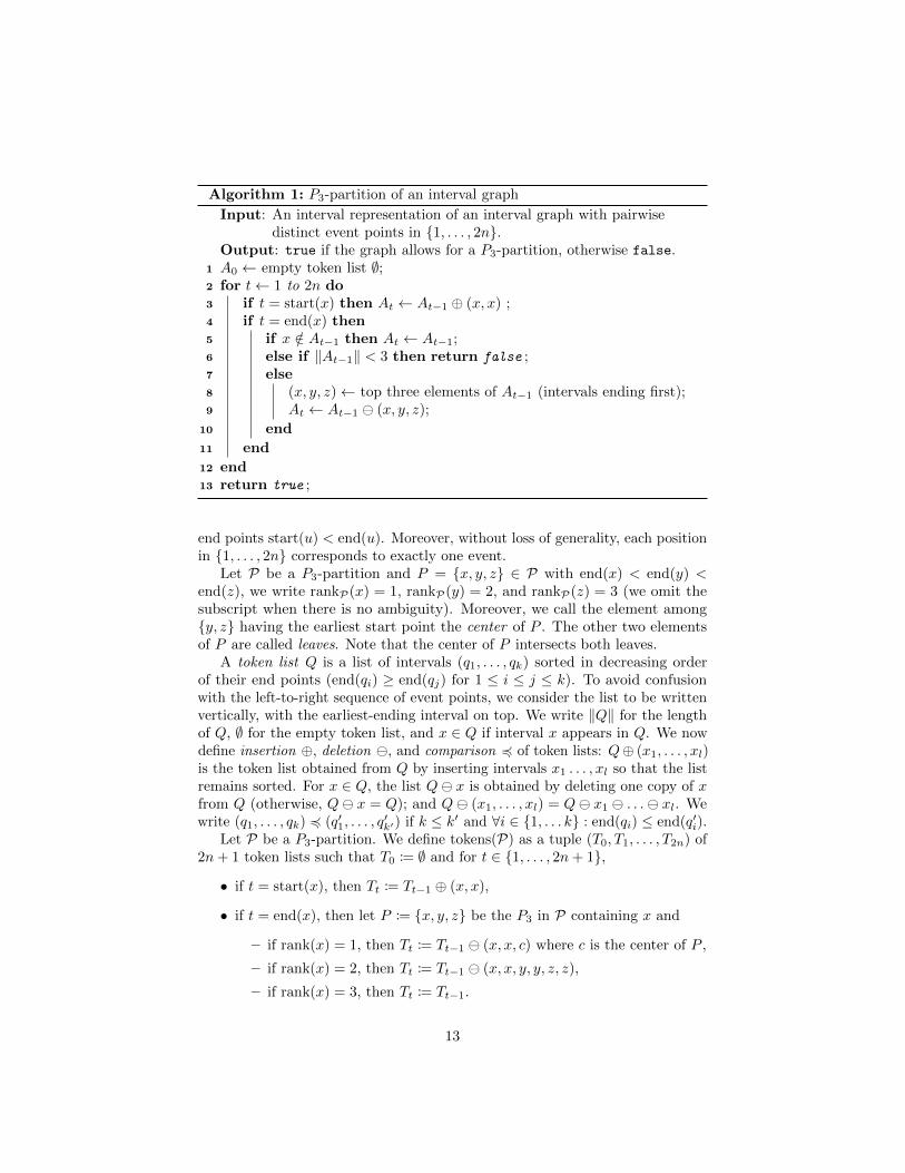
Algorithm 1: P3-partition of an interval graph
Input: An interval representation of an interval graph with pairwisedistinct event points in {1, . . . , 2n}.
Output: true if the graph allows for a P3-partition, otherwise false.1 A0 ← empty token list ∅;2 for t← 1 to 2n do3 if t = start(x) then At ← At−1 ⊕ (x, x) ;4 if t = end(x) then5 if x /∈ At−1 then At ← At−1;6 else if ‖At−1‖ < 3 then return false ;7 else8 (x, y, z)← top three elements of At−1 (intervals ending first);9 At ← At−1 (x, y, z);
10 end
11 end
12 end13 return true ;
end points start(u) < end(u). Moreover, without loss of generality, each positionin {1, . . . , 2n} corresponds to exactly one event.
Let P be a P3-partition and P = {x, y, z} ∈ P with end(x) < end(y) <end(z), we write rankP(x) = 1, rankP(y) = 2, and rankP(z) = 3 (we omit thesubscript when there is no ambiguity). Moreover, we call the element among{y, z} having the earliest start point the center of P . The other two elementsof P are called leaves. Note that the center of P intersects both leaves.
A token list Q is a list of intervals (q1, . . . , qk) sorted in decreasing orderof their end points (end(qi) ≥ end(qj) for 1 ≤ i ≤ j ≤ k). To avoid confusionwith the left-to-right sequence of event points, we consider the list to be writtenvertically, with the earliest-ending interval on top. We write ‖Q‖ for the lengthof Q, ∅ for the empty token list, and x ∈ Q if interval x appears in Q. We nowdefine insertion ⊕, deletion , and comparison 4 of token lists: Q⊕ (x1, . . . , xl)is the token list obtained from Q by inserting intervals x1 . . . , xl so that the listremains sorted. For x ∈ Q, the list Q x is obtained by deleting one copy of xfrom Q (otherwise, Q x = Q); and Q (x1, . . . , xl) = Q x1 . . . xl. Wewrite (q1, . . . , qk) 4 (q′1, . . . , q
′k′) if k ≤ k′ and ∀i ∈ {1, . . . k} : end(qi) ≤ end(q′i).
Let P be a P3-partition. We define tokens(P) as a tuple (T0, T1, . . . , T2n) of2n+ 1 token lists such that T0 := ∅ and for t ∈ {1, . . . , 2n+ 1},
• if t = start(x), then Tt := Tt−1 ⊕ (x, x),
• if t = end(x), then let P := {x, y, z} be the P3 in P containing x and
– if rank(x) = 1, then Tt := Tt−1 (x, x, c) where c is the center of P ,
– if rank(x) = 2, then Tt := Tt−1 (x, x, y, y, z, z),
– if rank(x) = 3, then Tt := Tt−1.
13

Note that in Figure 4, each token list Tt for P is equal to the respective At,except for T6 = (d, d) and T7 = (e, e, d, d).
To compare the token lists generated by Algorithm 1 to those induced by aP3-partition, we show a few properties for both types of lists.
Property 1. Let P be a P3-partition with tokens(P) = (T0, T1, . . . , T2n) andlet x be an interval with t := end(x). Then, one of the following is true:
i) x ∈ Tt−1, ‖Tt−1‖ ≥ 3, and ‖Tt‖ = ‖Tt−1‖ − 3 or
ii) x /∈ Tt−1 and Tt = Tt−1.
Moreover, in both cases, x /∈ Tt.
Proof. Let P ∈ P be the P3 containing x. Depending on the rank of x, we provethat either case (i) or (ii) applies.
If rank(x) = 1, then x is not the center of P . Let c be the center of P . Sincec is adjacent to x, it follows that start(c) < t. Since x ranks first, Tt−1 containstwice both elements x and c. Hence, ‖Tt−1‖ ≥ 4, and from the definition ofTt = Tt−1 (x, x, c) it follows that ‖Tt‖ = ‖Tt−1‖ − 3, we are thus in case (i).Moreover, only one copy of c remains in Tt.
If rank(x) = 2 and x is not the center, then let c be the center of P andy be the interval of the first rank in P . From the reasoning above, it followsthat Tt−1 contains once c and twice x but no y, implying that ‖Tt−1‖ ≥ 3.As Tt = Tt−1 (x, x, c, c, y, y), this implies that ‖Tt‖ = ‖Tt−1‖ − 3: we are incase (i).
If rank(x) = 2 and x is the center, then let P = {x, y, z} such that yranks first and z ranks third. Using the same reasoning as before it followsthat Tt−1 contains x once and z twice, but not y, implying that ‖Tt−1‖ ≥ 3.As Tt = Tt−1 (x, x, y, y, z, z), this implies that ‖Tt‖ = ‖Tt−1‖ − 3: we are incase (i).
Finally, if rank(x) = 3, then Tt−1 does not contain x (the last copies havebeen removed when the rank-2-interval ended), and Tt = Tt−1: we are in case (ii).
The fact that x /∈ Tt is clear in each case (all copies are removed whenx ∈ Tt−1, none is added).
Property 2. For any At defined by Algorithm 1 and x ∈ At, it holds thatstart(x) ≤ t < end(x). For any P3-partition P with tokens(P) = (T0, T1, . . . , T2n)and x ∈ Tt, it holds that start(x) ≤ t < end(x).
Proof. An element x is only added to a token list At or Tt when t = start(x), sothe inequality start(x) ≤ t is trivial in both cases. Consider now an interval xand t := end(x). We show that neither At nor Tt contain x, which suffices tocomplete the proof.
The fact that x /∈ Tt is already proven in Property 1. Moreover, if x /∈ At−1,then x /∈ At follows obviously.
Now, assume that x ∈ At−1. We inductively apply Property 2 to obtainthat for any y ∈ At−1, we have t− 1 < end(y) (note that the property is trivial
14

for A0). Hence, x is the interval with the earliest end point in At−1 (i. e., theinterval on top) and all of its copies(at most two) are removed from At−1 toobtain At in line 9 of Algorithm 1. It follows that x /∈ At.
Property 3. Let Q = (q1, . . . , qk) and Q′ = (q′1, . . . , q′k′) be two token lists such
that Q 4 Q′. Then for any qi ∈ Q, Q qi 4 Q′ q′k′ and for any interval x,Q⊕ x 4 Q′ ⊕ x.
Proof. For both insertion and deletion, the size constraint is clearly maintained(both list lengths respectively increase or decrease by 1). It remains to comparepairs of elements with the same index in both lists (such pairs are said to bealigned).
For the deletion case, qi is removed from Q. For any j 6= i, qj is now alignedwith either q′j (if j < i) or q′j−1 (if j > i). We have end(qj) ≤ end(q′j) sinceQ 4 Q′ and end(q′j) ≤ end(q′j−1) since Q′ is sorted. Hence, qj is aligned with aninterval in Q′ ending no later than qj itself.
We now prove the property for the insertion of x in both Q and Q′. Anelement q of Q or Q′ is said to be shifted if it is higher than the insertion pointof x (assuming that already-presentcopies of x in Q or Q′ are not shifted), this isequivalent to end(q) < end(x). Note that if some q′i is shifted but qi is not, thenend(q′i) < end(x) ≤ end(qi), a contradiction to end(q′i) ≥ end(qi). This impliesthat the insertion point of x in Q′ is not lower than the insertionpoint in Q.
Let q be an interval of Q⊕ x, now aligned with some q′ in Q′ ⊕ x. We provethat end(q′) ≥ end(q). Assume first that q = x, then either q′ = x, in whichcase trivially end(q′) ≥ end(q), or q′ 6= x. Then, q′ cannot be shifted (since x’sinsertion point is not lower in Q′ thanin Q), and end(q′) ≥ end(x) = end(q).
Assume now that q 6= x. Then, q = qi for some i. With Q 4 Q′, we haveend(q) ≤ end(q′i). If q′ = q′i then we directly have end(q) ≤ end(q′). Otherwise,exactly one of qi and q′i must be shifted. It cannot be q′i (the insertion point ofx is not lower in Q′ than in Q), henceqi is shifted and q′i is not. In Q we haveend(qi) < end(x), and in Q′ interval q′i must be placed directly below q′ andboth cannot occur higher than x (note that q′ = x ispossible), thus we haveend(q′i) ≥ end(q′) ≥ end(x). Overall, we indeed have end(q) ≤ end(q′).
Using the proven properties, we can put the token lists defined by a P3-partitioninto relation with the token lists generated by Algorithm 1.
The following two lemmas state that, on the one hand, if there is a P3-partition, then each token list created by Algorithm 1 is comparable with thecorresponding Tt, hence it always contains enough tokens to create the next list,up to A2n, and answer “true” in the end. On the other hand, if the algorithmreturns “true”, then it is indeed possible to construct a P3-partition using(indirectly) the triples of intervals removed from the token list to create the links.
Lemma 3. If an interval graph G has a P3-partition P, then, for all 0 ≤ t ≤ 2n,Algorithm 1 defines list At with Tt 4 At and ‖Tt‖ − ‖At‖ ≡ 0 (mod 3), wheretokens(P) = (T0, T1, . . . , T2n).
15
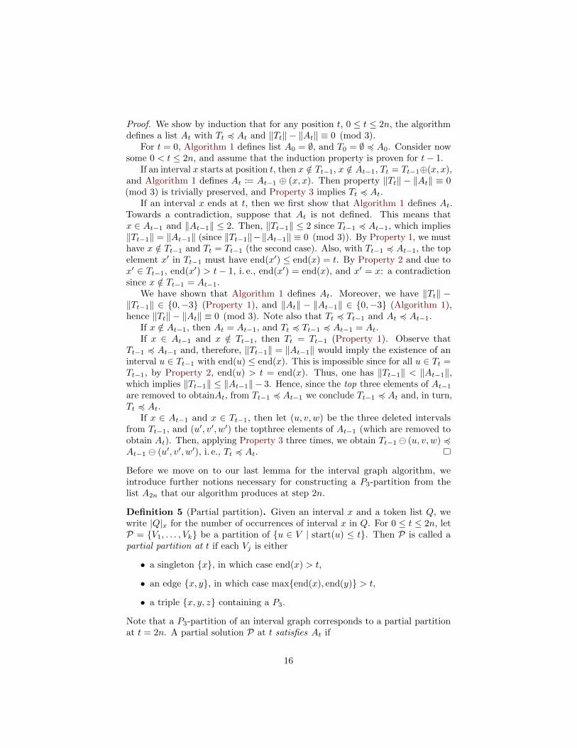
Proof. We show by induction that for any position t, 0 ≤ t ≤ 2n, the algorithmdefines a list At with Tt 4 At and ‖Tt‖ − ‖At‖ ≡ 0 (mod 3).
For t = 0, Algorithm 1 defines list A0 = ∅, and T0 = ∅ 4 A0. Consider nowsome 0 < t ≤ 2n, and assume that the induction property is proven for t− 1.
If an interval x starts at position t, then x /∈ Tt−1, x /∈ At−1, Tt = Tt−1⊕(x, x),and Algorithm 1 defines At := At−1 ⊕ (x, x). Then property ‖Tt‖ − ‖At‖ ≡ 0(mod 3) is trivially preserved, and Property 3 implies Tt 4 At.
If an interval x ends at t, then we first show that Algorithm 1 defines At.Towards a contradiction, suppose that At is not defined. This means thatx ∈ At−1 and ‖At−1‖ ≤ 2. Then, ‖Tt−1‖ ≤ 2 since Tt−1 4 At−1, which implies‖Tt−1‖ = ‖At−1‖ (since ‖Tt−1‖−‖At−1‖ ≡ 0 (mod 3)). By Property 1, we musthave x /∈ Tt−1 and Tt = Tt−1 (the second case). Also, with Tt−1 4 At−1, the topelement x′ in Tt−1 must have end(x′) ≤ end(x) = t. By Property 2 and due tox′ ∈ Tt−1, end(x′) > t− 1, i. e., end(x′) = end(x), and x′ = x: a contradictionsince x /∈ Tt−1 = At−1.
We have shown that Algorithm 1 defines At. Moreover, we have ‖Tt‖ −‖Tt−1‖ ∈ {0,−3} (Property 1), and ‖At‖ − ‖At−1‖ ∈ {0,−3} (Algorithm 1),hence ‖Tt‖ − ‖At‖ ≡ 0 (mod 3). Note also that Tt 4 Tt−1 and At 4 At−1.
If x /∈ At−1, then At = At−1, and Tt 4 Tt−1 4 At−1 = At.If x ∈ At−1 and x /∈ Tt−1, then Tt = Tt−1 (Property 1). Observe that
Tt−1 4 At−1 and, therefore, ‖Tt−1‖ = ‖At−1‖ would imply the existence of aninterval u ∈ Tt−1 with end(u) ≤ end(x). This is impossible since for all u ∈ Tt =Tt−1, by Property 2, end(u) > t = end(x). Thus, one has ‖Tt−1‖ < ‖At−1‖,which implies ‖Tt−1‖ ≤ ‖At−1‖ − 3. Hence, since the top three elements of At−1are removed to obtainAt, from Tt−1 4 At−1 we conclude Tt−1 4 At and, in turn,Tt 4 At.
If x ∈ At−1 and x ∈ Tt−1, then let (u, v, w) be the three deleted intervalsfrom Tt−1, and (u′, v′, w′) the topthree elements of At−1 (which are removed toobtain At). Then, applying Property 3 three times, we obtain Tt−1 (u, v, w) 4At−1 (u′, v′, w′), i. e., Tt 4 At.
Before we move on to our last lemma for the interval graph algorithm, weintroduce further notions necessary for constructing a P3-partition from thelist A2n that our algorithm produces at step 2n.
Definition 5 (Partial partition). Given an interval x and a token list Q, wewrite |Q|x for the number of occurrences of interval x in Q. For 0 ≤ t ≤ 2n, letP = {V1, . . . , Vk} be a partition of {u ∈ V | start(u) ≤ t}. Then P is called apartial partition at t if each Vj is either
• a singleton {x}, in which case end(x) > t,
• an edge {x, y}, in which case max{end(x), end(y)} > t,
• a triple {x, y, z} containing a P3.
Note that a P3-partition of an interval graph corresponds to a partial partitionat t = 2n. A partial solution P at t satisfies At if
16

• for any singleton {x} ∈ P we have |At|x = 2,
• for any edge {x, y} ∈ P with end(x) < end(y) we have |At|x = 0 and|At|y = 1, and
• for any triple {x, y, z} ∈ P we have |At|x = |At|y = |At|z = 0.
Note that, for any x ∈ At, since start(x) ≤ t < end(x) (Property 2), it followsthat x must be in a singleton or in an edge of any partial solution satisfying At.Moreover, for any t and x, y ∈ At with x 6= y, intervals x and y intersect (thereis an edge between them in the interval graph).
Lemma 4. Let G be an interval graph such that Algorithm 1 returns true on G.Then G admits a P3-partition.
Proof. We prove by induction that for any t such that Algorithm 1 defines At,there exists a partial solution at t satisfying At.
For t = 0, the partial solution ∅ satisfies A0. Assume now that for some t ≤ 2n,Algorithm 1 defines At, and that there exists a partial solution P at t − 1satisfying At−1.
First, if t = start(x) for some interval x, then let P ′ := P ∪ {{x}}. Thus,P ′ is now a partial solution at t (it partitions every interval with earlier startingpoint into singletons, edges and P3s) which satisfies At since by constructionof At by Algorithm 1, |At|x = 2.
Now assume that t = end(x) with x /∈ At−1. Then, in P, either x is part ofan edge {x, y} with end(y) > t, or x is part of a P3. In both cases, P ′ := P is apartial solution at t which satisfies At = At−1.
We now explore the case where t = end(x) with x ∈ At−1. Then, the topelement of At−1 must be x (no other interval u ∈ At−1 can have t−1 < end(u) ≤end(x)). Let y and z be the two elements below x in At−1. Then, by construction,At = At−1 (x, y, z) and end(x) ≤ end(y) ≤ end(z) ≤ end(u) for all u ∈ At.We create a partial solution P ′ at t depending on the number of occurrences ofx, y, and z in At−1.
If x = y (hence, |At−1|x = 2) and |At−1|z = 2, then P contains two single-tons {x} and {z}. Let P ′ := (P \ {{x}, {z}}) ∪ {{x, z}}. Then, P ′ is indeed apartial solution at t (since {x, z} is an edge with end(z) > t) that satisfies At,since |At|x = 0 and |At|z = 1.
If x = y (hence, |At−1|x = 2) and |At−1|z = 1, then P contains a single-ton {x} and an edge {z, u}. Also, note that |At−1|u = 0, that is, u /∈ At−1.Because there is an edge {x, z}, the triple {x, z, u} contains a P3. Let P ′ :=(P \ {{x}, {z, u}}) ∪ {{x, z, u}}. Then P ′ is a partial solution at t that satisfiesAt, since |At|x = |At|z = |At|u = 0.
If z = y (hence, |At−1|x = 1 and |At−1|z = 2), then similarly P containsan edge {x, u} and a singleton {z}: P ′ := (P \ {{x, u}, {z}}) ∪ {{x, z, u}} is apartial solution at t that satisfies At.
If y 6= x and y 6= z (hence, |At−1|x = 1 and |At−1|y = 1), and |At−1|z = 2,then P contains two edges {x, u} and {y, v} and a singleton {z}. Recall thatv, u /∈ At−1. Assume first that start(y) < start(x), then interval u intersects
17

y, and {y, u, v} contains a P3. Also, {x, z} forms an edge with |At|z = 1:define P ′ := (P \ {{x, u}, {y, v}, {z}}) ∪ {{y, u, v}, {x, z}}. In the case wherestart(x) < start(y), {x, u, v} contains a P3 and P ′ := (P \{{x, u}, {y, v}, {z}})∪{{x, u, v}, {y, z}} is a partial solution at t that satisfies At.
Finally, we have a similar situation when y 6= x, y 6= z and |At−1|z = 1: then,P contains three edges {x, u}, {y, v} and {z, w}. If start(y) < start(x), thenboth {y, u, v} and {x, z, w} contain P3s. Otherwise, {x, u, v} and {y, z, w} con-tain P3s. Thus, we define P ′ := (P\{{x, u}, {y, v}, {z, w}})∪{{y, u, v}, {x, z, w}}and P ′ := (P \ {{x, u}, {y, v}, {z, w}}) ∪ {{x, u, v}, {y, z, w}} respectively. Inboth cases, P ′ is a partial solution at t that satisfies At.
Overall, if Algorithm 1 returns true, then it defines A2n. According to theproperty we have proven, there exists a partial solution at t = 2n, hence G hasa P3-partition.
The above lemmas allow us to conclude the correctness of Algorithm 1.
Theorem 3. P3-Partition on interval graphs is solvable in O(n log n+m) time.
Proof. Let G be an interval graph. To prove the theorem, we show that Al-gorithm 1 returns true on G if and only if G has a P3-partition. The “onlyif” part is the statement of Lemma 4. For the “if” part, suppose that G hasa P3-partition P. Then Lemma 3 implies that Algorithm 1 defines list At atposition t = 2n, which means it returns true.
It remains to prove the running time bound. We first preprocess the input asfollows: in O(n+m) time, we can get an interval representation of an intervalgraph with n intervals that use start and end points in {1, . . . , n} [10, Section 8].We modify this representation so that each position is the start or end pointof at most one interval: first, for each interval, we add its start point to thebeginning of a list L and its end point to the end of L. We sort L using a stablesorting algorithm like counting sort in O(n) time. The result is a sorted list Lthat, for each position, contains first the start points and then the end points.Now, in O(n) time, we iterate over L and reassign each event points to its ownposition in {1, . . . , 2n} in the order of its appearance in L. At the same time,we build an 2n-element array B such that B[i] holds a pointer to the intervalstarting or ending at event point i (there is at most one such interval). It followsthat all preprocessing works in O(n+m) time.
After this preprocessing, each of the O(n) iterations for some t ∈ {1, . . . , 2n}of the loop in line 2 of Algorithm 1 is executed in O(log n) time: in constant time,we get the interval B[t] starting or ending at t and each operation on the tokenlist can be executed in O(log n) time if it is implemented as a balanced binarytree (note that only the current value of At need to be kept at each point, henceit is never necessary for the algorithm to make a copy of the whole token list).
18

3 Cographs
A cograph is a graph that does not contain a P4 (path on four vertices) as aninduced subgraph. Cographs allow for a so-called cotree to be computed in lineartime [9].
Definition 6. A cotree cot(G) of a cograph G = (V,E) is a rooted binarytree T = (VT , ET , r), r ∈ VT , where each internal node is assigned a label in{⊕,⊗} and the set of leaves corresponds to the original set V of vertices such that:
• A subtree consisting of a single leaf node corresponds to an induced sub-graph with a single vertex.
• A subtree rooted at a union node, labeled “⊕”, corresponds to the disjointunion of the subgraphs defined by the two children of that node.
• A subtree rooted at a join node, labeled “⊗”, corresponds to the join ofthe subgraphs defined by the two children of that node; that is, the unionof the two subgraphs with additional edges between every two verticescorresponding to leaves in different subtrees.
Consequently, the subtree rooted at the root r of cot(G) corresponds to G.
Using a dynamic programming approach on the cotree representation of thecograph, we can solve Star Partition in polynomial time.
Theorem 4. Star Partition can be solved in O(kn2) time on cographs.
Proof. Let (G = (V,E), s) be a Star Partition instance with G being a co-graph. Let T = (VT , ET , r) = cot(G) denote the cotree of G. Furthermore, forany node x ∈ VT , let T [x] denote the subgraph of G that corresponds to thesubtree of T rooted at x.
We define a dynamic programming table L as follows. For every node x ∈ VTand every non-negative integer c ≤ k, the table entry L[x, c] denotes the maximumnumber of leaves in T [x] that are covered by a center in T [x] when c verticesin T [x] are centers. Consequently, (G, s) is a yes-instance if and only if L[r, k] =ks. Now, let us describe how to compute L processing the cotree T bottom up.
Leaf nodes. For a leaf node x, either the only vertex v from T [x] is a centeror not. In both cases no leaf in T [x] is covered by v. Thus, L[x, 0] = L[x, 1] = 0and ∀c > 1 : L[x, c] = −∞.
Union nodes. Let x be a node labeled with “⊕” and let x1 and x2 be itschildren. Note that there is no edge between a vertex from T [x1] and a vertexfrom T [x2], neither in T [x] nor in any other subgraph of G corresponding toany T [x′], x′ ∈ VT . Thus, for every leaf v in T [x] that is covered by a center v′
from T [x], it holds that either both v and v′ are in T [x1] or both are in T [x2].Hence, it follows L[x, c] = maxc1+c2=c(L[x1, c1] + L[x2, c2]).
19
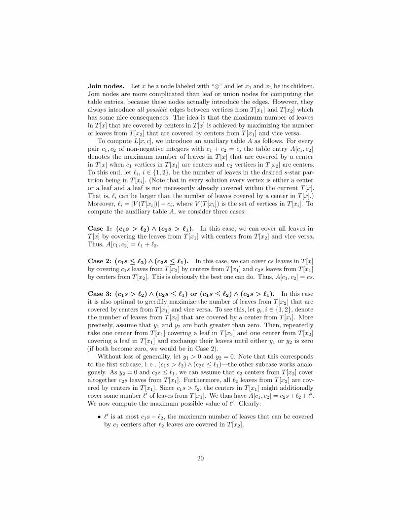
Join nodes. Let x be a node labeled with “⊗” and let x1 and x2 be its children.Join nodes are more complicated than leaf or union nodes for computing thetable entries, because these nodes actually introduce the edges. However, theyalways introduce all possible edges between vertices from T [x1] and T [x2] whichhas some nice consequences. The idea is that the maximum number of leavesin T [x] that are covered by centers in T [x] is achieved by maximizing the numberof leaves from T [x2] that are covered by centers from T [x1] and vice versa.
To compute L[x, c], we introduce an auxiliary table A as follows. For everypair c1, c2 of non-negative integers with c1 + c2 = c, the table entry A[c1, c2]denotes the maximum number of leaves in T [x] that are covered by a centerin T [x] when c1 vertices in T [x1] are centers and c2 vertices in T [x2] are centers.To this end, let `i, i ∈ {1, 2}, be the number of leaves in the desired s-star par-tition being in T [xi]. (Note that in every solution every vertex is either a centeror a leaf and a leaf is not necessarily already covered within the current T [x].That is, `i can be larger than the number of leaves covered by a center in T [x].)Moreover, `i = |V (T [xi])| − ci, where V (T [xi]) is the set of vertices in T [xi]. Tocompute the auxiliary table A, we consider three cases:
Case 1: (c1s > `2) ∧ (c2s > `1). In this case, we can cover all leaves inT [x] by covering the leaves from T [x1] with centers from T [x2] and vice versa.Thus, A[c1, c2] = `1 + `2.
Case 2: (c1s ≤ `2)∧ (c2s ≤ `1). In this case, we can cover cs leaves in T [x]by covering c1s leaves from T [x2] by centers from T [x1] and c2s leaves from T [x1]by centers from T [x2]. This is obviously the best one can do. Thus, A[c1, c2] = cs.
Case 3: (c1s > `2) ∧ (c2s ≤ `1) or (c1s ≤ `2) ∧ (c2s > `1). In this caseit is also optimal to greedily maximize the number of leaves from T [x2] that arecovered by centers from T [x1] and vice versa. To see this, let yi, i ∈ {1, 2}, denotethe number of leaves from T [xi] that are covered by a center from T [xi]. Moreprecisely, assume that y1 and y2 are both greater than zero. Then, repeatedlytake one center from T [x1] covering a leaf in T [x2] and one center from T [x2]covering a leaf in T [x1] and exchange their leaves until either y1 or y2 is zero(if both become zero, we would be in Case 2).
Without loss of generality, let y1 > 0 and y2 = 0. Note that this correspondsto the first subcase, i. e., (c1s > `2) ∧ (c2s ≤ `1)—the other subcase works analo-gously. As y2 = 0 and c2s ≤ `1, we can assume that c2 centers from T [x2] coveraltogether c2s leaves from T [x1]. Furthermore, all `2 leaves from T [x2] are cov-ered by centers in T [x1]. Since c1s > `2, the centers in T [x1] might additionallycover some number `′ of leaves from T [x1]. We thus have A[c1, c2] = c2s+ `2 + `′.We now compute the maximum possible value of `′. Clearly:
• `′ is at most c1s− `2, the maximum number of leaves that can be coveredby c1 centers after `2 leaves are covered in T [x2],
20

• `′ is at most `1 − c2s, the maximum number of leaves that are not alreadycovered by centers from T [x2], and
• `′ is at most L[x1, c1], the maximum number of leaves from T [x1] that canbe covered by centers from T [x1].
Hence, `′ ≤ min(c1s− `2, `1 − c2s, L[x1, c1])Conversely, for `′′ = min(c1s − `2, `1 − c2s, L[x1, c1]), it is possible for c1
centers in T [x1] to cover `′′ leaves in T [x1] and `2 leaves in T [x2], and for c2centers in T [x2] to cover c2s leaves in T [x1]. Here, the property that a join nodeintroduces all possible edges between the two subgraphs is crucial, because wecan therefore simply cover leaves from T [x1] by centers from T [x1] in an optimalway. (Each center from T [x1] can cover each leaf from T [x2] and vice versa.)So `′ ≥ `′′ = min(c2s− `1, `2 − c1s, L[x2, c2]). Overall,
A[c1, c2] =`1 + `2 if (c1s > `2) ∧ (c2s > `1)
cs if (c1s ≤ `2) ∧ (c2s ≤ `1)
c2s+ `2 + min(c1s− `2, `1 − c2s, L[x1, c1]) if (c1s > `2) ∧ (c2s ≤ `1)
c1s+ `1 + min(c2s− `1, `2 − c1s, L[x2, c2]) if (c1s ≤ `2) ∧ (c2s > `1).
Finally, we compute L[x, c] by considering the auxiliary table, that is,
L[x, c] = maxc1+c2=c
(A[c1, c2]).
The O(kn2) running time of this algorithm can be seen as follows: Computingthe cotree representation runs in linear time [9]. The table size of the dynamicprogram is bounded by O(kn)—there are O(n) nodes in the cotree and c ≤ k.Since V (T [xi]) corresponds to the set of leaf nodes of the subtree of T rootedin xi, the sizes |V (T [xi])| can be precomputed in linear time for each node xiof the cotree. Hence, computing a table entry costs at most O(n).
4 Bipartite permutation graphs
In this section, we show that Star Partition can be solved in O(n2) time onbipartite permutation graphs. The class of bipartite permutation graphs is theintersection of the class of bipartite graphs and the class of permutation graphs.An alternative characterization of bipartite permutation graphs can be givenusing strong orderings of the vertices of a bipartite graph:
Definition 7 (Spinrad et al. [28]). A strong ordering ≺ of the vertices of abipartite graph G = (U,W,E) is the union of a total order ≺U of U and a totalorder ≺W of W , such that, for all edges {u,w}, {u′, w′} in E with u, u′ ∈ U andw,w′ ∈W , u ≺ u′ and w′ ≺ w implies that there are edges {u,w′} and {u′, w}in E.
21

A graph is a bipartite permutation graph if and only if it is bipartite andthere is a strong ordering of its vertices; a strong ordering can be computed inlinear time [28].
In a bipartite graph G with vertex set U ∪W , if the subgraph induced bya size-(s + 1) vertex subset X ⊆ U ∪W contains an s-star, then this inducedsubgraph is a star—there is only one way to choose the star center. Thus, werefer to G[X] as a star. We denote by center(X) the center of the star G[X].Observe that the number kU of star centers in U and the number kW of starcenters in W are uniquely determined by the sizes |U | and |W | of the twoindependent vertex sets and by the number s of leaves in a star, since
|U | = kU + s · kW and |W | = kW + s · kU
and therefore
kU =|U | − |W | · s
1− s2and kW =
|W | − |U | · s1− s2
.
If these numbers are not positive integers, then G does not have an s-starpartition. Thus, we assume throughout this section that kU and kW are positiveintegers.
Our key to obtain star partitions on bipartite permutation graphs is astructural result that only a certain “normal form” of star partitions has tobe searched for. This paves the way to developing a dynamic programmingalgorithm exploiting these normal forms. We define these structural propertiesof an s-star partition of bipartite permutation graphs in the following.
Let (G, s) be a Star Partition instance, where G = (U,W,E) is a bipartitepermutation graph, ≺ is a strong ordering of the vertices, and 4 is the reflexiveclosure of ≺. For two vertex sets A,B, we also write A ≺ B if for all verticesv ∈ A and w ∈ B, we have v ≺ w.
Assume that G admits an s-star partition P. Let X ∈ P form a star. Bylm(X) (respectively by rm(X)), we denote the leftmost (that is, the minimum),respectively the rightmost (that is, the maximum) leaf of X with respect to ≺.The scope of star X is the set scope(X) := {v | xl 4 v 4 xr} containing allvertices from xl = lm(X) to xr = rm(X). The width of star X is the cardinalityof its scope, that is, width(X) := | scope(X)|. The width of P, width(P), is thesum of width(X) over all X ∈ P.
Let e = {u,w} and e′ = {u′, w′} be two edges. We say that e and e′ crosseach other if it holds that u ≺ u′ and w′ ≺ w or if it holds that u′ ≺ u andw ≺ w′. The edge-crossing number of two stars X,Y ∈ P is the number of pairsof crossing edges e, e′ with respect to the given strong order ≺ where e is anedge of X and e′ is an edge of Y . The edge-crossing number #edge-crossings(P)of P is the sum of the edge-crossing numbers over all pairs of stars X 6= Y ∈ P.
We identify the possible configurations of two stars, depending on the relativepositions of their leaves and centers, see Figure 5. Among those, the followingtwo configurations are favorable: Given X,Y ∈ P, we say that X and Y are
• non-crossing if their edge-crossing number is zero;
22

Non-crossing
Interleaving
Configuration I
Configuration III
Configuration II
Configuration IV
Figure 5: Possible interactions between two stars of a partition. Centers aredrew black. The four possible configurations of star centers and scopes thatare neither non-crossing nor interleaving are labeled I to IV. By Lemma 5, anypartition containing one of the configurations I to IV can be edited to reducethe score (see the thick gray edges).
• interleaving if center(X) ∈ scope(Y ) and center(Y ) ∈ scope(X);
We say that P is good if any two stars X 6= Y ∈ P are either non-crossing or in-terleaving. We define the score of P as the tuple (width(P),#edge-crossings(P)).We use the lexicographical order to compare scores.
These definitions allow us to observe the following property and show anormal form of star partitions in bipartite permutation graphs.
Property 4. Let u0 ≺ u1 and w0 ≺ w1 be four vertices such that edges {u0, w1}and {u1, w0} are in G. Then, G has edges {u0, w0} and {u1, w1} and, for anyedge e crossing one (respectively both) edge(s) in {{u0, w0}, {u1, w1}}, e crossesone (respectively both) edge(s) in {{u0, w1}, {u1, w0}}.
Proof. The existence of the edges {u0, w0} and {u1, w1} is a direct consequenceof Definition 7. Let e = {u,w} be an edge crossing {u0, w0} and/or {u1, w1}.We consider the cases where u ≺ u0 and where u0 ≺ u ≺ u1 (the case u1 ≺ ubeing symmetrical to u ≺ u0).
If u ≺ u0, then w0 ≺ w, and e crosses both {u0, w0} and {u1, w0}. Also, ife crosses {u1, w1}, then e also crosses {u0, w1}, which proves the property forthis case.
If u0 ≺ u ≺ u1, then if e crosses {u0, w0}, then e also crosses {u0, w1}. Ife crosses {u1, w1}, then e also crosses {u1, w0}. Overall, the property is thusproven for all cases.
Our main structural lemma now is the following.
23
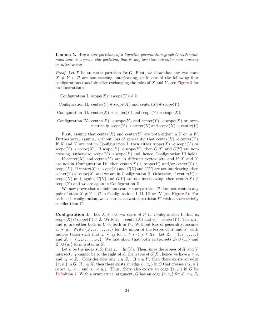
Lemma 5. Any s-star partition of a bipartite permutation graph G with mini-mum score is a good s-star partition, that is, any two stars are either non-crossingor interleaving.
Proof. Let P be an s-star partition for G. First, we show that any two starsX 6= Y ∈ P are non-crossing, interleaving, or in one of the following fourconfigurations (possibly after exchanging the roles of X and Y , see Figure 5 foran illustration):
Configuration I. scope(X) ∩ scope(Y ) 6= ∅;
Configuration II. center(Y ) ∈ scope(X) and center(X) 6∈ scope(Y );
Configuration III. center(X) ≺ center(Y ) and scope(Y ) ≺ scope(X);
Configuration IV. center(X) ≺ scope(Y ) and center(Y ) ≺ scope(X) or, sym-metrically, scope(Y ) ≺ center(X) and scope(X) ≺ center(Y ).
First, assume that center(X) and center(Y ) are both either in U or in W .Furthermore, assume, without loss of generality, that center(X) ≺ center(Y ).If X and Y are not in Configuration I, then either scope(X) ≺ scope(Y ) orscope(Y ) ≺ scope(X). If scope(X) ≺ scope(Y ), then G[X] and G[Y ] are non-crossing. Otherwise, scope(Y ) ≺ scope(X) and, hence, Configuration III holds.
If center(X) and center(Y ) are in different vertex sets and if X and Yare not in Configuration IV, then center(X) ∈ scope(Y ) and/or center(Y ) ∈scope(X). If center(X) ∈ scope(Y ) and G[X] and G[Y ] are not interleaving, thencenter(Y ) /∈ scope(X) and we are in Configuration II. Otherwise, if center(Y ) ∈scope(X) and, again, G[X] and G[Y ] are not interleaving, then center(X) /∈scope(Y ) and we are again in Configuration II.
We now prove that a minimum-score s-star partition P does not contain anypair of stars X 6= Y ∈ P in Configurations I, II, III or IV (see Figure 5). Foreach such configuration, we construct an s-star partition P ′ with a score strictlysmaller than P.
Configuration I. Let X,Y be two stars of P in Configuration I, that is,scope(X) ∩ scope(Y ) 6= ∅. Write xc = center(X) and yc = center(Y ). Then, xcand yc are either both in U or both in W . Without loss of generality, assumexc ≺ yc. Write {z1, z2, . . . , z2s} for the union of the leaves of X and Y , withindices taken such that zi ≺ zj for 1 ≤ i < j ≤ 2s. Let Zl = {z1, . . . , zs}and Zr = {zs+1, . . . , z2s}. We first show that both vertex sets Zl ∪ {xc} andZr ∪ {yc} form a star in G.
Let k be the index such that zk = lm(Y ). Then, since the scopes of X and Yintersect, zk cannot be to the right of all the leaves of G[X], hence we have k ≤ s,and zk ≺ Zr. Consider now any z ∈ Zr. If z ∈ Y , then there exists an edge{z, yc} in G. If z ∈ X, then there exists an edge {z, xc} in G that crosses {zk, yc}(since zk ≺ z and xc ≺ yc). Thus, there also exists an edge {z, yc} in G byDefinition 7. With a symmetrical argument, G has an edge {z, xc} for all z ∈ Zl.
24

It follows that the vertex sets X ′ = Zl ∪ {xc} and Y ′ = Zr ∪ {yc} both formstars in G.
We now compare the widths of G[X ′] and G[Y ′] to the widths of the originalstars G[X] and G[Y ]. Let w be the total number of elements between z1 and z2s,that is, the cardinality of the vertex set {u | z1 4 u 4 z2s} = scope(X)∪scope(Y ).Then, using the fact that the scopes of X ′ and Y ′ are disjoint and included in asize-w set, we have
width(X ′) + width(Y ′) ≤ w= | scope(X)|+ | scope(Y )| − | scope(X) ∩ scope(Y )|< width(X) + width(Y ).
We can thus construct an s-star partition P ′ = (P \ {X,Y }) ∪ {X ′, Y ′} suchthat width(P ′) < width(P), that is, with strictly smaller score. Thus, no pair ofstars in the minimum-score s-star partition P may be in Configuration I.
Configuration II. Let X,Y be two stars of P in Configuration II, i. e.,center(Y ) ∈ scope(X) and center(X) 6∈ scope(Y ). Write xc = center(X)and yc = center(Y ). Then yc ≺ rm(X) and either xc ≺ scope(Y ) or scope(Y ) ≺xc. We only consider the case xc ≺ scope(Y ); the case scope(Y ) ≺ xc worksanalogously.
Let v = rm(X) be the rightmost vertex of the leaves of the star G[X]. First,G contains the edge {xc, yc} since the star G[Y ] has at least one leaf u withxc ≺ u and yc ≺ v, and G contains the edges {xc, v} and {yc, u}. Now, considerany vertex u ∈ Y \ {center(Y )}. Then, the edge {xc, v} crosses the edge {u, yc},since xc ≺ u and yc ≺ rm(X). The graph G contains the edges {xc, yc} and{v, u}. Thus, the vertex sets X ′ = (X \ {v}) ∪ {yc} and Y ′ = (Y \ {yc}) ∪ {v}both form stars in G.
We now compare the widths of G[X ′] and G[Y ′] to the widths of the originalstars G[X] and G[Y ].
Since yc ≺ v, one has width(X ′) ≤ width(X) − 1. Obviously, width(Y ) =width(Y ′). We can thus construct an s-star partition P ′ = (P\{X,Y })∪{X ′, Y ′}with width(P ′) < width(P), that is, with strictly smaller score. Therefore, nopair of stars in the s-star partition P may be in Configuration II.
Configuration III. Let X,Y be two stars of P in Configuration III. Let xc :=center(X) and yc := center(Y ) and assume, without loss of generality, that xc ≺yc. Then, scope(Y ) ≺ scope(X). Thus, all edges of G[X] cross all edges of G[Y ].Hence, there exists an edge {xc, y} for each leaf y of G[Y ], and an edge {yc, x} foreach leaf x of G[X]. Defining X ′ = (X \ {xc})∪{yc} and Y ′ = (Y \ {xc})∪{yc},we thus have two stars G[X ′] and G[Y ′] with the same width as G[X] and G[Y ],respectively. Hence, the s-star partition P ′ = (P \ {X,Y }) ∪ {X ′, Y ′} has thesame width as P.
We now show that #edge-crossings(P ′) < #edge-crossings(P). We write BX
(respectively BY , BX′ , and BY ′) for the branches of the corresponding star, that
25
center(Y ) lm(X) rm(X)
center(X) lm(Y ) rm(Y )
center(Y ′) lm(X ′) rm(X ′)
center(X ′)lm(Y ′) rm(Y ′)
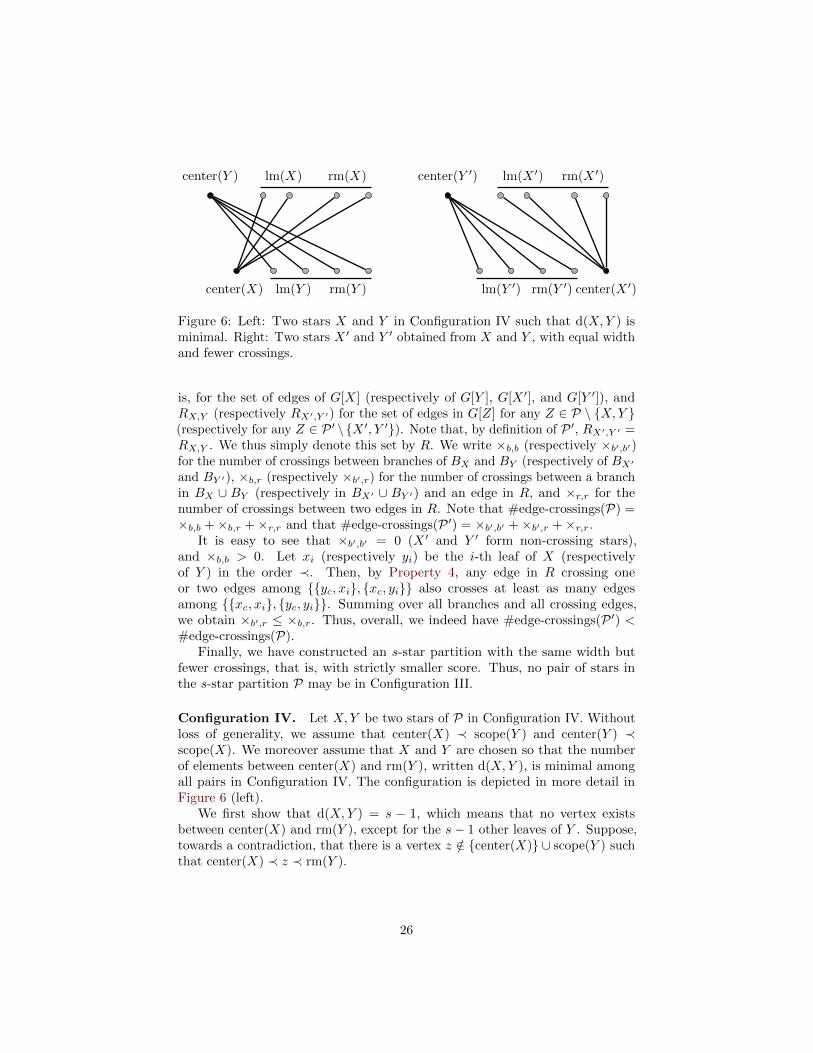
Figure 6: Left: Two stars X and Y in Configuration IV such that d(X,Y ) isminimal. Right: Two stars X ′ and Y ′ obtained from X and Y , with equal widthand fewer crossings.
is, for the set of edges of G[X] (respectively of G[Y ], G[X ′], and G[Y ′]), andRX,Y (respectively RX′,Y ′) for the set of edges in G[Z] for any Z ∈ P \ {X,Y }(respectively for any Z ∈ P ′ \{X ′, Y ′}). Note that, by definition of P ′, RX′,Y ′ =RX,Y . We thus simply denote this set by R. We write ×b,b (respectively ×b′,b′)for the number of crossings between branches of BX and BY (respectively of BX′
and BY ′), ×b,r (respectively ×b′,r) for the number of crossings between a branchin BX ∪ BY (respectively in BX′ ∪ BY ′) and an edge in R, and ×r,r for thenumber of crossings between two edges in R. Note that #edge-crossings(P) =×b,b +×b,r +×r,r and that #edge-crossings(P ′) = ×b′,b′ +×b′,r +×r,r.
It is easy to see that ×b′,b′ = 0 (X ′ and Y ′ form non-crossing stars),and ×b,b > 0. Let xi (respectively yi) be the i-th leaf of X (respectivelyof Y ) in the order ≺. Then, by Property 4, any edge in R crossing oneor two edges among {{yc, xi}, {xc, yi}} also crosses at least as many edgesamong {{xc, xi}, {yc, yi}}. Summing over all branches and all crossing edges,we obtain ×b′,r ≤ ×b,r. Thus, overall, we indeed have #edge-crossings(P ′) <#edge-crossings(P).
Finally, we have constructed an s-star partition with the same width butfewer crossings, that is, with strictly smaller score. Thus, no pair of stars inthe s-star partition P may be in Configuration III.
Configuration IV. Let X,Y be two stars of P in Configuration IV. Withoutloss of generality, we assume that center(X) ≺ scope(Y ) and center(Y ) ≺scope(X). We moreover assume that X and Y are chosen so that the numberof elements between center(X) and rm(Y ), written d(X,Y ), is minimal amongall pairs in Configuration IV. The configuration is depicted in more detail inFigure 6 (left).
We first show that d(X,Y ) = s − 1, which means that no vertex existsbetween center(X) and rm(Y ), except for the s− 1 other leaves of Y . Suppose,towards a contradiction, that there is a vertex z /∈ {center(X)} ∪ scope(Y ) suchthat center(X) ≺ z ≺ rm(Y ).
26

Assume first that z is the center of a star G[X ′] with X ′ ∈ P. Then,scope(X) ≺ scope(X ′), since X and X ′ cannot be in Configuration I or III.Moreover, we have center(X) ≺ z ≺ scope(Y ) since, otherwise, z ∈ scope(Y ) andY and X ′ would be in Configuration II. Hence, X ′ and Y are in configuration IV(with center(X ′) ≺ scope(Y ), center(Y ) ≺ scope(X ′)), and d(X ′, Y ) < d(X,Y ),which is a contradiction.
Now assume that z is a leaf of a star G[Y ′] with Y ′ ∈ P. First compareY and Y ′: scope(Y ′) ∩ scope(Y ) = ∅ since, otherwise, Y and Y ′ would be inConfiguration I. Using z ≺ rm(Y ), it follows that scope(Y ′) ≺ scope(Y ). Thisimplies that center(Y ′) ≺ center(Y ) ≺ scope(X) since, otherwise, Y ′ and Ywould be in Configuration III. We now compare X and Y ′. We have alreadyseen that center(Y ′) ≺ scope(X). Also, center(X) /∈ scope(Y ′) since, otherwise,Y ′ and X would be in Configuration II. Using center(X) ≺ z, we thus havecenter(X) ≺ scope(Y ′), which implies that X and Y ′ are in Configuration IVwith d(X,Y ′) < d(X,Y ), which is a contradiction. We conclude that no vertexother than the leaves of Y may exist between center(X) and rm(Y ).
We now construct an s-star partition with score strictly less than P . To thisend, let X0 = X \ {center(X)} and Y0 = Y \ {rm(Y )}. First observe that Gcontains the edge {center(X), center(Y )} since there is an edge in G[X] andan edge in G[Y ] crossing each other. Hence, Y ′ = Y0 ∪ {center(X)} forms astar. Now, consider any vertex u ∈ X0. The edge {center(X), u} crosses theedge {center(Y ), rm(Y )} and, therefore, G contains the edge {rm(Y ), u}. Thus,X ′ = X0 ∪ {rm(Y )} forms a star. For an illustration, see Figure 6 (right). Also,X ′ and Y ′ are non-crossing (X ′ is completely to the right of Y ′).
We now compare the widths of G[X ′] and G[Y ′] to the widths of the originalstars G[X] and G[Y ]. Obviously, width(X ′) = width(X). Moreover, sinced(X,Y ) = s − 1, it follows that width(Y ′) = width(Y ) = s. Hence, the s-starpartition P ′ = (P \ {X,Y }) ∪ {X ′, Y ′} has the same width as P.
Since the widths have not changed, we have to show that #edge-crossings(P ′) <#edge-crossings(P). We introduce the same notations as in Configuration III:Let BX (respectively BY , BX′ , and BY ′) be the set of branches of the corre-sponding star, that is, the set of edges in G[X] (respectively in G[Y ], G[X ′],and G[Y ′]), and let RX,Y (respectively RX′,Y ′) be the set of edges in G[Z] for anyZ ∈ P \ {X,Y } (respectively for any Z ∈ P ′ \ {X ′, Y ′}). Note that by definitionof P ′, RX′,Y ′ = RX,Y , and we thus simply denote this set by R. Furthermore,let ×b,b (respectively ×b′,b′) be the number of crossings between branches of BX
and BY (respectively between branches of BX′ and BY ′), let ×b,r (respectively×b′,r) be the number of crossings between a branch in BX ∪BY (respectively inBX′ ∪BY ′) and an edge in R, and let ×r,r be the number of crossings betweentwo edges in R. Note that #edge-crossings(P) = ×b,b + ×b,r + ×r,r and that#edge-crossings(P ′) = ×b′,b′ +×b′,r +×r,r. Then, it is easy to see that ×b′,b′ = 0(X ′ and Y ′ form non-crossing stars), and ×b,b > 0.
We now show that ×b′,r ≤ ×b,r. First recall that no edge in R has an endpoint between center(X) and rm(Y ). We consider the branches in BX′∪BY ′ and,for each, give a unique edge in BX ∪BY crossing the same edges of R. For anyleaf x of X ′, any r ∈ R crossing {center(X ′), x} must also cross {center(X), x}.
27
For the leftmost branch of Y ′, any r ∈ R crossing {center(X), center(Y )} mustalso cross {rm(Y ), center(Y )}. For any other branch b = {center(Y ), y} ofY ′, any r ∈ R must also cross the same branch b of Y ′. Overall, we indeedhave ×b′,r ≤ ×b,r, which implies #edge-crossings(P ′) < #edge-crossings(P).
Altogether, we have shown that a minimum-score s-star partition P containingpairs of stars in Configurations I to IV leads to a contradiction, since, in this case,we could find an s-star partition of lower score, which is a contradiction.
As a consequence of Lemma 5, we obtain the following corollary.
Corollary 1. Let P be an s-star partition of a bipartite permutation graph Gwith minimum score. Then, for each star X ∈ P, there is at most one Y ∈ Psuch that X and Y are interleaving, and for all Z ∈ P \ {X,Y }, X and Z arenon-crossing.
Proof. Since P has minimum score, for any Y ∈ P \ {X}, G[X] and G[Y ] areeither interleaving or non-crossing.
Any star interleaving with G[X] contains center(x) in its scope. If thereexist at least two such stars in P, then their scopes intersect and they are inConfiguration I, which is impossible by Lemma 5.
We now informally describe a dynamic programming algorithm for decidingwhether a bipartite graph G = (U,W,E) allows for a good s-star partition. Itbuilds up a solution following the strong ordering of the graph from left to right.A partial solution can be extended in three ways only: either (i) a star is addedwith the center in U , or (ii) a star is added with the center in W , or (iii) twointerleaving stars are added. The algorithm can thus compute, for any givennumber of centers in U and in W , whether it is possible to partition the leftmostvertices of U and W in one of the three ways (i)–(iii). This algorithm leads tothe following result.
Theorem 5. Star Partition can be solved in O(n2) time on bipartite permu-tation graphs.
Proof. Let (G, s) denote a Star Partition instance, where G = (U,W,E) is abipartite permutation graph. Furthermore, let U = {u1, u2, . . . , ukU
} and W ={w1, w2, . . . , wkW
} such that ui ≺ uj (respectively wi ≺ wj) implies i < j forsome fixed strong ordering ≺. We describe a dynamic programming algorithmthat finds a good s-star partition P . The idea is to use the fact that a star from Pis either interleaving with exactly one other star from P or it does not cross anyother star from P (see Lemma 5 and Corollary 1). In both cases, the part ofthe graph that lies entirely to the left of the star (of the two interleaving starsrespectively) with respect to the strong ordering must have an s-star partitionon its own. This is clearly also true for the part of the graph that lies entirely tothe right, but we do not need this for the proof.
Informally, an entry T (x, y) of our binary dynamic programming table T istrue if and only if x stars with centers from U and y stars with centers from Wcan “consecutively cover” the correspondingly large part of the graph from the
28
left side of the strong ordering. Formally, the binary dynamic programmingtable T is defined as
T (x, y) =
1 if G[{u1, u2, . . . , ux+s·y, w1, w2, . . . , wy+s·x}]
has an s-star partition,
0 otherwise.
Initialize the table T by:
T (0, 1) =
{1 if G[{u1, u2, . . . , us, w1}] contains an s-star,
0 otherwise,
T (1, 0) =
{1 if G[{u1, w1, w2, . . . , ws}] contains an s-star,
0 otherwise, and
T (1, 1) =
1 if G[{u1, u2, . . . , us+1, w1, w2, . . . , ws+1}]
contains disjoint s-stars,
0 otherwise.
Update the table T for all 1 < x ≤ kU and 1 < y ≤ kW by
T (x, y) =
1 if one of the following holds:
(a) T (x, y− 1) = 1 and G[{ux+s·(y−1)+1, ux+s·(y−1)+2, . . . , ux+s·(y−1)+s,w(y−1)+s·x+1}] contains an s-star,
(b) T (x−1, y) = 1 and G[{u(x−1)+s·y+1, wy+s·(x−1)+1, wy+s·(x−1)+2, . . . ,wy+s·(x−1)+s}] contains an s-star,
(c) T (x− 1, y− 1) = 1 and G[{u(x−1)+s·(y−1)+1, . . . , u(x−1)+s·(y−1)+s+1,w(y−1)+s·(x−1)+1, . . . , w(y−1)+s·(x−1)+s+1}] contains disjoint s-stars.
0 otherwise.
Concerning the running time, first, a strong ordering of the vertices can becomputed in linear time [28]. Second, the table in the dynamic program hasO(k2) entries and initialization as well as updating works in O(s2) time. Hence,the total running time is O(k2 · s2) = O(n2).
Concerning the correctness of the algorithm, we show that T (kU , kV ) istrue if and only if there is a good s-star partition and, hence, if and only ifthere is an s-star partition. To this end, consider an s-star partition P ′ forG′ := G[{u1, u2, . . . , ux+s·y, w1, w2, . . . , wy+s·x}] with minimum score. Nowthere are three simple cases:
Case (a). The rightmost vertex of G′ in W is a center of a non-crossing starin P ′ and, hence, G[{u1, u2, . . . , ux+s·(y−1), w1, w2, . . . , wy−1+s·x}] has an s-starpartition.
29

Case (b). The rightmost vertex of G′ in U is a center of a non-crossing starin P ′ and, hence, G[{u1, u2, . . . , ux−1+s·y, w1, w2, . . . , wy+s·(x−1)}] has an s-starpartition.
Case (c). The rightmost vertex of G′ in U and G′s rightmost vertex in Ware leaves of two interleaving stars. Due to Corollary 1, none of the other starsfrom P ′ is crossing these two stars. It follows that G[{u1, u2, . . . , ux−1+s·(y−1),w1, w2, . . . , wy−1+s·(x−1}] has an s-star partition.
Note that the rightmost vertex of G′ in U can only be a leaf of a non-crossingstar in P ′ if the rightmost vertex of G′ in W is the center and vice versa. Oth-erwise, the corresponding star is clearly not non-crossing. Hence, these casesare already covered by (a) and (b). Furthermore, neither the rightmost vertexof G′ in U nor in W can be a center of an interleaving star from P ′, becauseboth are rightmost with respect to the strong ordering and, thus, interleaving isimpossible. Thus we considered all cases and the update process is correct.
5 Split graphs
A split graph is a graph whose vertices can be partitioned into a clique (that is,a complete subgraph) and an independent set (that is, a subgraph with onlyisolated vertices). Remarkably, split graphs are the only graph class where wecould show that P3-Partition is solvable in polynomial time, but that StarPartition for s ≥ 3 is NP-hard.
More precisely, we solve P3-Partition on split graphs by reducing it tofinding a restricted form of factor in an auxiliary graph; herein, a factor ofa graph G is a spanning subgraph of G (that is, a subgraph containing allvertices). This graph factor problem then can be solved in polynomial time [11].Alternatively, we can also solve the problem by reducing it to finding perfectmatchings (Theorem 6).
Let G = (C ∪ I, EC ∪E) be a split graph where (C,EC) is a clique, I inducesan independent set, and B = (C ∪ I, E) forms a bipartite graph over C and I.Note that if |C| + |I| is not a multiple of 3, or if |I| > 2|C|, then G triviallyhas no P3-partition. We thus assume that |C|+ |I| (and hence 2|C| − |I|) is amultiple of 3, and that 2|C| − |I| ≥ 0.
First, we show how a P3-partition of a split graph is related to a specificfactor of the bipartite graph B. Assume that G admits a partition into P3s andlet P denote the set of edges in the partition. There are three types of P3s:
(i) a P3 consisting of three clique vertices,
(ii) a P3 consisting of two clique vertices and one independent set vertex, and
(iii) a P3 consisting of one clique vertex and two independent set vertices.
Note that, for each P3, we can assume that the edges are selected so that eachindependent set vertex is incident with at most one edge in P . In particu-
30

lar, this implies that the two clique vertices in Type (ii) are adjacent in thecorresponding P3. This leads to the following definition.
Definition 8. A factor F of the bipartite graph B is feasible if, in F , everyindependent set vertex has degree one, every clique vertex has degree zero, oneor two, and there are at least as many degree-zero clique vertices as degree-oneclique vertices.
It turns out that Definition 8 is necessary and sufficient for obtaining aP3-partition.
Lemma 6. A split graph G admits a partition into P3s if and only if there existsa feasible factor of its bipartite graph B.
Proof. Assume that there is a partition of G into P3s with edge set P such thateach vertex in I is incident with exactly one edge in P . Let PE := P ∩ E bethe subset of edges of the partition which connect vertices from C with verticesfrom I, and let F := (C ∪ I, PE) be the corresponding factor of B = (C ∪ I, E).
Each independent set vertex in I has degree one in F (since it is adjacent toexactly one edge in P , which is also in PE). Each clique vertex v in C belongsto a P3 from P . Depending on the type of this P3, in F , vertex v can havedegree zero (Type (i) or (ii), note that we assume each independent set vertexto be incident with at most one edge in P ), degree one (Type (ii)), or degreetwo (Type (iii)). Let n(i) (respectively n(ii)) denote the number of P3s of Type (i)(respectively (ii)). It remains to show that the number of degree-zero cliquevertices is equal to or greater than the number of degree-one clique vertices: Thenumber of degree-zero vertices is n(ii) + 3n(i), and the number of degree-onevertices is n(ii), hence the difference is positive. Thus, F is feasible.
Conversely, let F = (C ∪ I, PE) be a feasible factor of B. Then we par-tition G into P3s as follows. For each degree-two clique vertex v in C, add{v, x, y} to P where x and y are the neighbors of v in F . For each degree-oneclique vertex v in C, add {v, x, y} to P , where x is v’s neighbor in F and y is anarbitrary degree-zero clique vertex (there are enough such vertices). The numberof remaining degree-zero vertices in C is thus a multiple of 3: these vertices aresimply grouped up in arbitrary triples Add these triples to P . Overall, due tothe degree constraints, P is a P3-partition of G.
Cornuejols [11] shows that finding a feasible factor in B can be solved inpolynomial time by reducing it to finding disjoint edges and triangles in acorresponding auxiliary graph. Nevertheless, we show in the following how toreduce the problem to finding perfect matchings. To this end, we formulate anice property that a feasible factor in B must fulfill:
Property 5. Let F = (C ∪ I, P ∩ E) be a feasible factor of the bipartitegraph B = (C ∪ I, E). Let q and r be two non-negative integers such thatr ∈ {0, 1} and (2|C| − |I|)/3 = 2q + r. Then, in F , the number n1 of degree-onevertices in C is 2i+ r for some i, 0 ≤ i ≤ q. In particular, n1 ≤ (2|C| − |I|)/3.
31

Proof. Let n0, n1, and n2 be the number of degree-zero, degree-one, and degree-two clique vertices in F . Then, n0 + n1 + n2 = |C| (all clique vertices havedegree 0, 1 or 2), n1 + 2n2 = |I| (vertices in I have degree 1). Rearranging andresolving variable n2 yields
3n1 = 2|C| − |I| − 2(n0 − n1). (2)
As mentioned, 2|C| − |I| is a multiple of three (as well as |C|+ |I|). Note thatn0 − n1, which is positive because F is feasible, is a multiple of three because itequals the number of clique vertices in P3s of Type (i). Let j be an integer with(n0 − n1)/3 = j. Then, together with (2), we obtain that
n1 =2|C| − |I|
3− 2 · n0 − n1
3= 2q + r − 2j.
The last statement is satisfied since 2q + r = (2|C| − |I|)/3 and j ≥ 0.
To be able use a perfect matching algorithm to solve our problem, we firstreduce it to a restricted variant of the graph factor problem: We add an additionalvertex z to the bipartite graph B, and connect it to all vertices in C. We callthis graph B′. Now, the following lemma states that B′ can be used to find afeasible factor for B.
Lemma 7. The bipartite graph B = (C ∪ I, E) admits a feasible factor if andonly if graph B′ = (C ∪ I ∪ {z}, E ∪ {{z, c} | c ∈ C}) has a factor satisfying thefollowing degree constraints: (1) Every vertex in I has degree one, (2) everyvertex in C has degree zero or two, and (3) the added vertex z has degree 2i+ r,where r ∈ {0, 1} such that there is an integer q with (2|C| − |I|)/3 = 2q + r andi ∈ {0, 1, . . . , q}.
Proof. Assume that B admits a feasible factor F = (C ∪ I, PE). Then F ′ =(C ∪ I ∪ {z}, PE) is a factor of B′. For each degree-one vertex v ∈ C, we addedge {v, z} to factor F ′. By Property 5, we thus add 2i+ r edges, with 0 ≤ i ≤ q.It is easy to verify that the degree constraints stated in the lemma are satisfied.
Conversely, let F ′ be a factor for graph B′ where every independent setvertex has degree one, every clique vertex has degree zero or two, and vertex zhas degree 2i+ r with i ∈ {0, 1, . . . , q}. If we delete from F ′ all edges incidentto vertex z, then we obtain a feasible factor F for B where the number n1 ofdegree-one clique vertices is the original degree of z, that is,
n1 = 2i+ r ≤ (2|C| − |I|)/3. (3)
Since each independent set vertex still has degree one, the number of degree-two clique vertices is (|I| − n1)/2, and the number of degree-zero clique ver-tices is n0 = |C| − n1 − (|I| − n1)/2 = (2|C| − |I| − n1)/2. The differencebetween the number of degree-zero and the number of degree-one vertices isn0 − n1 = (2|C| − |I| − 3n1)/2, which is non-negative by using (3).
32
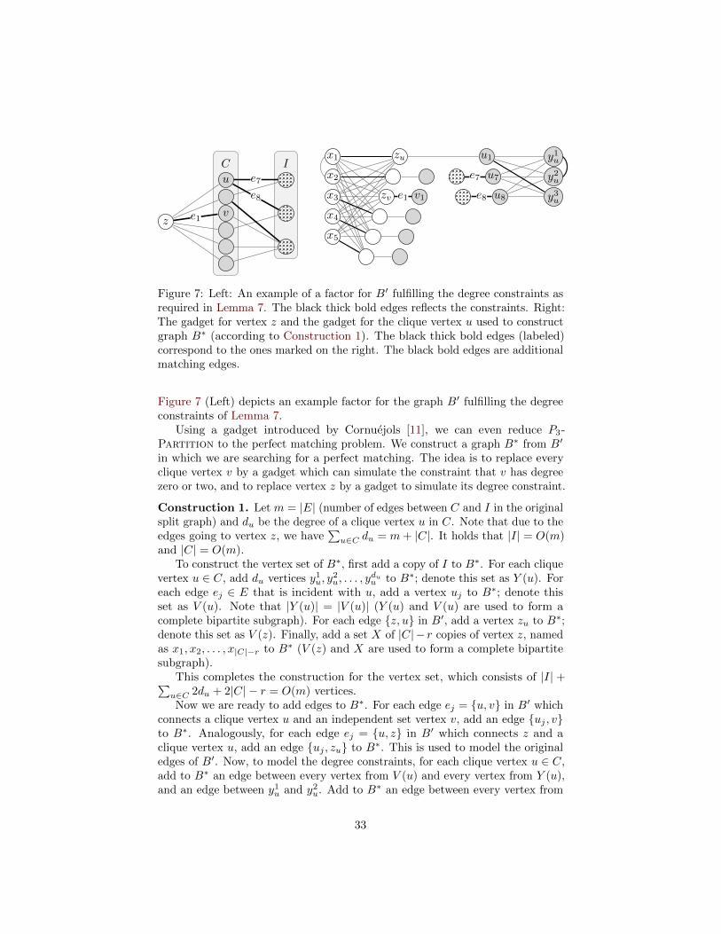
z
C
u
v
Ie7
e8
e1
zu
zv
x1
x2
v1x3
x4
x5
u1
u7
u8
y1u
y2u
y3u
e7
e8e1
Figure 7: Left: An example of a factor for B′ fulfilling the degree constraints asrequired in Lemma 7. The black thick bold edges reflects the constraints. Right:The gadget for vertex z and the gadget for the clique vertex u used to constructgraph B∗ (according to Construction 1). The black thick bold edges (labeled)correspond to the ones marked on the right. The black bold edges are additionalmatching edges.
Figure 7 (Left) depicts an example factor for the graph B′ fulfilling the degreeconstraints of Lemma 7.
Using a gadget introduced by Cornuejols [11], we can even reduce P3-Partition to the perfect matching problem. We construct a graph B∗ from B′
in which we are searching for a perfect matching. The idea is to replace everyclique vertex v by a gadget which can simulate the constraint that v has degreezero or two, and to replace vertex z by a gadget to simulate its degree constraint.
Construction 1. Let m = |E| (number of edges between C and I in the originalsplit graph) and du be the degree of a clique vertex u in C. Note that due to theedges going to vertex z, we have
∑u∈C du = m+ |C|. It holds that |I| = O(m)
and |C| = O(m).To construct the vertex set of B∗, first add a copy of I to B∗. For each clique
vertex u ∈ C, add du vertices y1u, y2u, . . . , y
duu to B∗; denote this set as Y (u). For
each edge ej ∈ E that is incident with u, add a vertex uj to B∗; denote thisset as V (u). Note that |Y (u)| = |V (u)| (Y (u) and V (u) are used to form acomplete bipartite subgraph). For each edge {z, u} in B′, add a vertex zu to B∗;denote this set as V (z). Finally, add a set X of |C|− r copies of vertex z, namedas x1, x2, . . . , x|C|−r to B∗ (V (z) and X are used to form a complete bipartitesubgraph).
This completes the construction for the vertex set, which consists of |I| +∑u∈C 2du + 2|C| − r = O(m) vertices.Now we are ready to add edges to B∗. For each edge ej = {u, v} in B′ which
connects a clique vertex u and an independent set vertex v, add an edge {uj , v}to B∗. Analogously, for each edge ej = {u, z} in B′ which connects z and aclique vertex u, add an edge {uj , zu} to B∗. This is used to model the originaledges of B′. Now, to model the degree constraints, for each clique vertex u ∈ C,add to B∗ an edge between every vertex from V (u) and every vertex from Y (u),and an edge between y1u and y2u. Add to B∗ an edge between every vertex from
33

V (z) and every vertex from X. Finally, for each integer i with 1 ≤ i ≤ q, addto B∗ edge {x2i−1, x2i}.
The overall number of edges in B∗ is (m+ |C|) +∑
u∈C(du)2 + |C|(|C| − r) +|C|+ q ≤ (m+ |C|)2 + |C|2 +O(m) = O(m2). This finishes the construction.
Figure 7 (Right), shows the gadget constructed for a clique vertex and thegadget for vertex z. Now, we show how the constructed graph B∗ can be usedto find a factor for B′ satisfying the specific degree constraints as specified inLemma 7.
Lemma 8. Graph B∗ constructed according to Construction 1 admits a perfectmatching if and only if graph B′ admits a factor F ′ satisfying the condition that(1) Every vertex in I has degree one, (2) every vertex in C has degree zero ortwo, and (3) the added vertex z has degree 2i + r, where r ∈ {0, 1} such thatthere is an integer q with (2|C| − |I|)/3 = 2q + r and i ∈ {0, 1, . . . , q}.
Proof. Let M be a perfect matching for B∗. We construct a factor F ′ =(C∪I∪{z}, P ′E) for B′. For each edge {uj , v} ∈M which connects an independentset vertex v, add to P ′E edge {u, v}. For each edge {zu, uj} ∈M which connectsvertices in V (z) and V (u), u ∈ C, add to P ′E edge {z, u}.
We show that F ′ is a factor for B∗ satisfying the properties stated in thelemma. Obviously, every independent set vertex u ∈ I has degree one. Considera clique vertex u ∈ C. By the construction of graph B∗, in order to match allvertices in Y (u), either (i) every vertex in Y (u) has to be matched to a vertex inV (u) or (ii) y1u and y2u are matched together while every vertex in Y (u)\{y1u, y2u}is matched to exactly one vertex in V (u). This implies that either no vertexor exactly two vertices in V (u) are matched to some vertices which are notfrom Y (u). Thus, v has either degree zero or degree two in F ′.
Analogously, by the construction of graph B∗, in order to match all vertices inX which has size |C|−r, exactly i pairs of vertices in X can be left without beingmatched to any vertex in V (z) where 0 ≤ i ≤ q (note that only the first 2q verticesare connected by a path). This implies that exactly |C| − (|C| − r− 2i) = 2i+ rvertices from V (z) are matched to vertices that are not from X. Thus, z hasdegree 2i+ r.
Conversely, assume that B′ admits a factor F ′ satisfying the above properties.We show that the following construction yields a perfect matching M for B∗.
For each edge ej = {u, v} in F ′ that connects a clique vertex u and anindependent set vertex v, add to M edge {uj , v}. For each edge ej = {z, u}in F ′ that connects vertex z with a clique vertex u, add to M edge {zu, uj}.
For each clique vertex u ∈ C, let R(u) ⊆ V (u) be the set of vertices whichare not yet matched by M . We need to match all vertices in R(u). Dependingon whether u has degree zero or two in F ′, |V (u)| − |R(u)| is either zero or two,and |Y (u)| − |R(u)| = |V (u)| − |R(u)|. Moreover, B∗[V (u) ∪ Y (u)| contains acomplete bipartite graph for V (u) and Y (u). If |R(u)| = |V (u)| (which meansthat u has degree zero in F ′), then add to M edges connecting exactly onevertex of R(u) and one vertex of Y (u); otherwise, |R(u)| = |V (u)| − 2: addedge {y1u, y2u} to M , and edges connecting exactly one vertex of R(u) and one
34
vertex of Y (u) \ {y1u, y2u}. Analogously, let R(z) ⊆ V (z) be the set of verticesin V (z) which are not yet matched by M . By assumption, there is an integer i,0 ≤ i ≤ q such that |V (z)| − |R(z)| = 2i + r. Since |X| = |V (z)| − r, we have|X| − |R(z)| = 2i. Moreover, B∗[V (z) ∪X| contains a complete bipartite graphfor V (z) and X. Thus, for each 1 ≤ k ≤ i, add edge {x2k−1, x2k} to M , andadd edges connecting exactly one vertex of R(z) and one vertex of X to matchvertices of Rz and of V ′z \ {x1, x2, . . . , x2i}. It is easy to verify that M is indeeda perfect matching.
We now have gathered all ingredients to show Theorem 6.
Theorem 6. Star Partition on split graphs is solvable in O(m2.5) time fors = 2.
Proof. Let G = (C ∪ V,CE ∪ E) be a split graph with m being the number ofedges in E. Let B′ = (C ∪ V ∪ {z}, E ∪ {{z, v} | v ∈ C}) be a bipartite graphover C and I ∪ {z}. Let B∗ be computed from B′ using Construction 1. ByLemmas 6 to 8, G admits a P3-partition if and only if B∗ admits a perfectmatching. Since deciding whether a graph with s vertices and t edges has aperfect matching can be done in O(t
√s) time [27, Theorem 16.4] and since B∗
has O(m) vertices and O(m2) edges, deciding whether G has a P3-partition canbe done in O(m2.5) time.
In contrast, we can show that Star Partition is NP-hard for each s ≥ 3 by areduction from Exact Cover by s-Sets.
Theorem 7. Star Partition on split graphs is NP-hard for s ≥ 3.
Proof. We show that it is NP-hard to find an s-star partition of a split graphvia reduction from Exact Cover by s-Sets [16] (illustrated in Figure 8).
Exact Cover by s-SetsInput: A finite set U and a collection S of size-s subsets of U .Question: Is there a subcollection S ′ ⊆ S that partitions U (each element
of U is contained in exactly one subset in S ′)?
Given (U,S) with |U | = sn and |S| = m ≥ n where n,m ∈ N, we construct asplit graph G = (C ∪ I, E) as follows: The vertex set consists of a clique C andan independent set I. The clique C contains a vertex for each subset in S, theindependent set I contains a vertex for each element of U . For each S ∈ S thecorresponding vertex in C is adjacent to the s vertices in I that correspond tothe elements of S. Moreover, let q, r ∈ N such that m− n = (s− 1)q + r. Weadd q dummy vertices to both C and I and connect every dummy vertex in Cwith all other vertices in C and uniquely with one of the dummy vertices in I.Finally, we add one more dummy vertex to C and another s− r dummy verticesto I. This last dummy in C is connected to all other vertices in C and to eachof the s− r dummies in I. Note that each dummy vertex in I has degree one.The above construction can be carried out in polynomial time.
35

IU
CS
Figure 8: Reduction from Exact Cover by s-Sets to Star Partition withs = 3. Dummy vertices are in the light gray area and non-dummy vertices are inthe dark gray area. The 3-star partition for the constructed graph G is indicatedby thick edges.
Now, let S ′ ⊆ S be a partition of U . Then we can partition G into stars ofsize s in the following way: For each S ∈ S ′, we choose the star containing thevertex from C corresponding to S and the vertices in I corresponding to theelements of S. Moreover, each of the dummy vertices in I is put together withits neighboring dummy in C and filled up to a star of size s with the remainingnon-dummy vertices in C corresponding to the subsets in S \ S ′. Indeed, thevalues of q and r are chosen in a way that guarantees that this is possible.Since S ′ partitions U , we get a valid s-star partition of G.
Conversely, in any s-star partition of G, all dummy vertices in I are groupedtogether into an s-star with their one dummy neighbor in C and the respectivenumber of other non-dummy vertices from C. The values of q and r are such thatthere are exactly n non-dummy vertices left in C together with the s · n verticesin I corresponding to U . It follows that each remaining non-dummy vertex in Cforms a star with its s neighbors in I, which yields a partition of U .
6 Grid graphs
In this section, we show that P3-Partition is NP-hard even on grid graphswith maximum degree three, thus strengthening a result of Ma lafiejski andZylinski [22] and Monnot and Toulouse [23], who showed that P3-Partition isNP-complete on planar bipartite graphs of maximum degree three.
A grid graph is a graph with a vertex set V ⊆ N× N and edge set {{u, v} |u = (i, j) ∈ V, v = (k, `) ∈ V, |i− k|+ |j − `| = 1}. That is, its vertices can begiven integer coordinates such that every pair of vertices is joined by an edge ifand only if their coordinates differ by 1 in exactly one dimension.
To show NP-hardness of P3-Partition on grid graphs, we exploit the abovementioned result of Ma lafiejski and Zylinski [22] and Monnot and Toulouse [23]and find a suitable embedding of planar graphs into grid graphs while maintain-ing the property of a graph having a P3-partition. This allows us to prove thefollowing.
36

v w⇐⇒
v w
(a) Case 1: Vertex v and vertex w are covered by the same P3 (which implies that one vertex isan endpoint and the other vertex is an internal point of the P3).
v w⇐⇒
v w
(b) Case 2: Vertex v and vertex w are covered by different P3s (vertex v and/or vertex w canalso be internal vertices).
Figure 9: All possibilities of two vertices v and w participating in a P3-partitionif they are joined by an edge or a path on three other degree-two vertices. Edgesparticipating in the same P3 are grouped together in a gray background.
Theorem 8. P3-Partition is NP-hard on grid graphs of maximum degreethree.
Towards proving Theorem 8, the following observation helps us embed planargraphs into grid graphs: it allows us to replace edges by paths on 3i new verticesfor any i ∈ N.
Observation 5. Let G be a graph, e = {v, w} be an edge of G, and G′ be thegraph obtained by removing the edge e from G and by connecting v and w usinga path on three new vertices. Then, G has a P3-partition if and only if G′ hasone.
Note that the correctness of Observation 5 is proven by Figure 9, which enumer-ates all possible cases.
We can now prove Theorem 8 by showing that G has a P3-partition if andonly G′ has, where G′ is the graph obtained from a planar graph G of maximumdegree three using the following construction.
Construction 2. Let G be a planar n-vertex graph of maximum degree three.Using a polynomial-time algorithm of Rosenstiehl and Tarjan [26] we obtain acrossing-free rectilinear embedding of G into the plane such that:
1. Each vertex is represented by a horizontal line.
2. Each edge is represented by a vertical line.
3. All lines end at integer coordinates with integers in O(n).
37

a b
cd
(a) A planar graph G.
a
b
d
c
(b) A rectilinear embed-ding of G.
a′
c′
d′
b′
(c) The grid graph G′ ob-tained from G.
Figure 10: Various embeddings of a planar graph. In the rectilinear embedding inFigure 10b, horizontal lines represent vertices of G, while vertical lines representits edges. In Figure 10c, every intersection of a line with a grid point is avertex, but only the vertices corresponding to vertices in Figure 10a are shown.The horizontal lines of the rectilinear embedding are now replaced by pathshighlighted in gray.
4. If two vertices are joined by an edge, then the vertical line representingthis edge ends on the horizontal lines representing the vertices.
Figure 10b illustrates such an embedding. Without loss of generality, every endpoint of a line lies on another line. Now, in polynomial time, we obtain a gridgraph G′ from the rectilinear embedding, as follows:
1. We multiply all coordinates by six (see Figure 10c).
2. Every point in the grid touched by a horizontal line that represents avertex v of G becomes a vertex in G′. The horizontal path resulting fromthis horizontal line we denote by P (v) (indicated by a gray background inFigure 10c).
3. For each vertical line, all its grid points become vertices in G′, except forthe third point from the bottom horizontal line that we bypass by addinga bend of five vertices to the vertical line (see Figure 10c).
4. With each vertex v in G, we associate the vertex v′ of G′ that lies on P (v)and has degree three. There is at most one such vertex. If no such vertexexists, then we arbitrarily associate with v one of the end points of P (v).
Proof of Theorem 8. Since Construction 2 runs in polynomial time, it remainsto prove that a graph G has a P3-partition if and only if the graph G′ obtainedby Construction 2 has. By Observation 5, it is sufficient to verify that everyedge e := {u, v} in G is replaced by a path p between u′ and v′ in G′ whosenumber of inner vertices is divisible by three. To this end, we partition thepath p into two parts: one part consists of the subpaths pu, pv of p that lie onP (u) and P (v), respectively. Note that each of pu and pv might consist only of
38

one vertex, as seen for the path from d′ to a′ in Figure 10c. The other part is apath pe that connects pu to pv. We consider pe not to contain the vertices of puor pv. Hence, pe contains no vertices of any horizontal paths.
The number of inner vertices of p shared with the horizontal paths pu and pvis divisible by three (it is possibly zero) since all coordinates that start or endpaths are divisible by three (in fact, by six). Herein, note that we do not countthe vertices u′ and v′ lying on pu or pv, respectively.
Moreover, the number of vertices on pe is also divisible by three: the numberof vertices on a strictly vertical path ps connecting pu with pv would leave aremainder of two when divided by three (as the two vertices on pu and pv arenot considered to be part of ps). However, our added bend of five new verticesmakes pe by four vertices longer compared to ps. Hence, the number of verticeson pe is also divisible by three. It follows that the total number of inner verticesof p is divisible by three.
7 Chordal graphs
A graph is chordal if every induced subgraph containing a cycle of length atleast four also contains a triangle, that is, a cycle of length three. We showthat P3-Partition restricted to chordal graphs is NP-hard (in contrast to thepolynomial-time solvability on split graphs which form a subclass of chordalgraphs) by reduction from 3-Dimensional Matching. More precisely, we usethe construction that Dyer and Frieze [14] provided to show that P3-Partitionis NP-complete and observe that we can triangulate the resulting graph whilemaintaining the correctness of the reduction.
3-Dimensional Matching (3DM)Input: Pairwise disjoint sets R,B, Y with |R| = |B| = |Y | = q and a set of
triples T ⊆ R×B × Y .Question: Does there exist a perfect 3-dimensional matching M ⊆ T , that is,|M | = q and each element of R ∪B ∪ Y occurs in exactly one triple of M?
Dyer and Frieze [14] introduced Construction 3 described below and illustratedin Figure 11). Using it as a reduction from the NP-complete restriction of 3DMto planar graphs [15], they proved that P3-Partition restricted to bipartiteplanar graphs is NP-complete.
Construction 3. Let (R,B, Y, T ⊆ R × B × Y ) with |R| = |B| = |Y | = qbe an instance of 3DM. Construct a graph G = (V,E) as follows: For eachelement a ∈ R ∪ B ∪ Y , create two vertices ua, u
′a and connect them by an
edge {ua, u′a}. We call ua an element-vertex and u′a a pendant-vertex. Foreach triple t = (r, b, y) ∈ T , create three vertices vtr, v
tb, v
ty. We call these three
vertices triple-vertices. Make triple-vertex vtb adjacent to both vtr and vty. Also
39
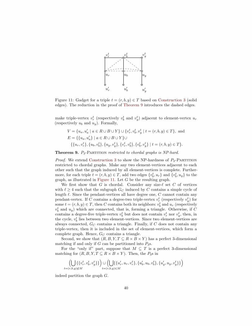
vtr vtb vty
ur
u′r
ub
u′b
uy
u′y
Figure 11: Gadget for a triple t = (r, b, y) ∈ T based on Construction 3 (solidedges). The reduction in the proof of Theorem 9 introduces the dashed edges.
make triple-vertex vtr (respectively vtb and vty) adjacent to element-vertex ur(respectively ub and uy). Formally,
V = {ua, u′a | a ∈ R ∪B ∪ Y } ∪ {vtr, vtb, vty | t = (r, b, y) ∈ T}, and
E = {{ua, u′a} | a ∈ R ∪B ∪ Y }∪{{ur, vtr}, {ub, vtb}, {uy, vty}, {vtr, vtb}, {vtb, vty} | t = (r, b, y) ∈ T}.
Theorem 9. P3-Partition restricted to chordal graphs is NP-hard.
Proof. We extend Construction 3 to show the NP-hardness of P3-Partitionrestricted to chordal graphs. Make any two element-vertices adjacent to eachother such that the graph induced by all element-vertices is complete. Further-more, for each triple t = (r, b, y) ∈ T , add two edges {vtb, ur} and {vtb, uy} to thegraph, as illustrated in Figure 11. Let G be the resulting graph.
We first show that G is chordal. Consider any size-` set C of verticeswith ` ≥ 4 such that the subgraph GC induced by C contains a simple cycle oflength `. Since the pendant-vertices all have degree one, C cannot contain anypendant-vertex. If C contains a degree-two triple-vertex vtr (respectively vty) forsome t = (r, b, y) ∈ T , then C contains both its neighbors: vtb and ur (respectivelyvtb and uy) which are connected, that is, forming a triangle. Otherwise, if Ccontains a degree-five triple-vertex vtb but does not contain vtr nor vty, then, inthe cycle, vtb lies between two element-vertices. Since two element-vertices arealways connected, GC contains a triangle. Finally, if C does not contain anytriple-vertex, then it is included in the set of element-vertices, which form acomplete graph. Hence, GC contains a triangle.
Second, we show that (R,B, Y, T ⊆ R×B × Y ) has a perfect 3-dimensionalmatching if and only if G can be partitioned into P3s.
For the “only if” part, suppose that M ⊆ T is a perfect 3-dimensionalmatching for (R,B, Y, T ⊆ R×B × Y ). Then, the P3s in(⋃
t=(r,b,y)/∈M
{{vtr, vtb, vty}})∪(⋃
t=(r,b,y)∈M
{{u′r, ur, vtr}, {u′b, ub, vtb}, {u′y, uy, vty}})
indeed partition the graph G.
40
For the “if” part, suppose that G has a partition P into P3s. We firstenumerate the possible centers of the P3s. Since each pendant-vertex is onlyadjacent to its element-vertex, every element-vertex is the center of a P3 thatcontains a pendant-vertex. We call such a P3 an element-P3. For each triple t =(r, b, y) ∈ T , neither vtr nor vty can be the center of a P3 since they are adjacent toonly one vertex which is not already a center (namely vtb). Thus, any P3 whichis not an element-P3 must have vertex vtb as a center for some t = (r, b, y) ∈ T .We call such a P3 a triple-P3 corresponding to t.
Now, consider a triple t = (r, b, y) ∈ T . If there exists a triple-P3 correspond-ing to t (that is, with center vtb), then its two leaves can only be vtr and vty (sinceutr, utb, and uty are centers). Otherwise, each of the three triple-vertices vtr, vtb,and vty must be a leaf of an element-P3 centered on ur, ub, and uy. Indeed, thereis only one way to match the three triple-vertices to these three element-vertices,that is, by using the edges {vtr, ur}, {vtb, ub} and {vty, uy}. As a consequence,the leaves of the element-P3 centered on ua are u′a and vta for some triple tcontaining a.
It remains to show that the triples with no corresponding triple-P3 in Pform a perfect 3-dimensional matching M for (R,B, Y, T ⊆ R×B × Y ). Notethat for each element a ∈ R ∪ B ∪ Y , the element-P3 centered in ua uses atriple-vertex vta for some triple t containing a, which means that no triple-P3
in P corresponds to t. Hence, t ∈ M and element a is matched by t. Now, itremains to show that every element is matched at most once. Suppose for thesake of contradiction that there is an element a ∈ R ∪B ∪ Y which is matchedat least twice. To this end, let vta be a triple-vertex that together with ua andu′a forms an element-P3. Thus, t ∈ M . Furthermore, let t′ be another triplein M that matches a. Since t′ has no corresponding triple-P3 in P , there is anelement-P3 containing vt
′
a . But then, vt′
a must form an element-P3 together withua and u′a, which is a contradiction.
8 Conclusion
We close with three open questions for future research. What is the complexityof Star Partition for s ≥ 2 on permutation graphs? What is the complexity ofStar Partition for s ≥ 3 on interval graphs? Are there other important graphclasses (not necessarily perfect ones) where Star Partition is polynomial-timesolvable?
Acknowledgments. Rene van Bevern was supported by the Russian Founda-tion for Basic Research (RFBR), project 16-31-60007 mol a dk, at NovosibirskState University, and by the German Research Foundation (DFG), project DAPA(NI 369/12), at TU Berlin. Robert Bredereck was supported by the DFG, projectPAWS (NI 369/10). Laurent Bulteau and Gerhard J. Woeginger were supportedby the Alexander von Humboldt Foundation, Bonn, Germany, while visitingTU Berlin. Jiehua Chen was supported by the Studienstiftung des DeutschenVolkes. Vincent Froese was supported by the DFG, project DAMM (NI 369/13).
41

This work started at the yearly research retreat of the group “Algorithms andComputational Complexity TU Berlin” in March 2013, held in Bad Schandau,Germany.
References
[1] K. Asdre and S. D. Nikolopoulos. NP-completeness results for some problemson subclasses of bipartite and chordal graphs. Theoretical Computer Science,381(1-3):248–259, 2007.
[2] F. Berman, D. Johnson, T. Leighton, P. W. Shor, and L. Snyder. Generalizedplanar matching. Journal of Algorithms, 11(2):153–184, 1990.
[3] R. van Bevern, C. Komusiewicz, H. Moser, and R. Niedermeier. Measuringindifference: Unit Interval Vertex Deletion. In Proceedings of the 36thInternational Workshop on Graph-Theoretic Concepts in Computer Science(WG ’10), volume 6410 of LNCS, pages 232–243. Springer, 2010.
[4] R. van Bevern, R. Bredereck, J. Chen, V. Froese, R. Niedermeier, and G. J.Woeginger. Network-based vertex dissolution. SIAM Journal on DiscreteMathematics, 29(2):888–914, 2015.
[5] R. van Bevern, M. Mnich, R. Niedermeier, and M. Weller. Interval schedulingand colorful independent sets. Journal of Scheduling, 18(5):449–469, 2015.
[6] A. Brandstadt, V. B. Le, and J. P. Spinrad. Graph Classes: A Survey,volume 3 of SIAM Monographs on Discrete Mathematics and Applications.SIAM, 1999.
[7] J. Chalopin and D. Paulusma. Packing bipartite graphs with covers ofcomplete bipartite graphs. Discrete Applied Mathematics, 168:40–50, 2014.
[8] E. Cohen and M. Tarsi. NP-completeness of graph decomposition problems.Journal of Complexity, 7(2):200–212, 1991.
[9] D. G. Corneil, Y. Perl, and L. Stewart. A linear recognition algorithm forcographs. SIAM Journal on Computing, 14(4):926–934, 1985.
[10] D. G. Corneil, S. Olariu, and L. Stewart. The LBFS structure and recognitionof interval graphs. SIAM Journal on Discrete Mathematics, 23(4):1905–1953,2009.
[11] G. Cornuejols. General factors of graphs. Journal of Combinatorial Theory.Series B, 45(2):185–198, 1988.
[12] E. Dahlhaus and M. Karpinski. Matching and multidimensional matchingin chordal and strongly chordal graphs. Discrete Applied Mathematics, 84(1-3):79–91, 1998.
42

[13] K. M. J. De Bontridder, B. V. Halldorsson, M. M. Halldorsson, C. A. J.Hurkens, J. K. Lenstra, R. Ravi, and L. Stougie. Approximation algorithmsfor the test cover problem. Mathematical Programming, 98(1-3):477–491,2003.
[14] M. E. Dyer and A. M. Frieze. On the complexity of partitioning graphs intoconnected subgraphs. Discrete Applied Mathematics, 10(2):139–153, 1985.
[15] M. E. Dyer and A. M. Frieze. Planar 3DM is NP-complete. Journal ofAlgorithms, 7(2):174–184, 1986.
[16] M. R. Garey and D. S. Johnson. Computers and Intractability: A Guide tothe Theory of NP-Completeness. Freeman, 1979.
[17] M. C. Golumbic. Algorithmic Graph Theory and Perfect Graphs. Annals ofDiscrete Mathematics. Elsevier, Amsterdam, Boston, Paris, 2004.
[18] D. G. Kirkpatrick and P. Hell. On the complexity of general graph factorproblems. SIAM Journal on Computing, 12(3):601–608, 1983.
[19] A. W. J. Kolen, J. K. Lenstra, C. H. Papadimitriou, and F. C. R. Spieksma.Interval scheduling: A survey. Naval Research Logistics, 54(5):530–543,2007.
[20] A. Kosowski, M. Ma lafiejski, and P. Zylinski. Parallel processing subsystemswith redundancy in a distributed environment. In Proceedings of the 6thInternational Conference on Parallel Processing and Applied Mathematics(PPAM ’05), volume 3911 of LNCS, pages 1002–1009. Springer, 2006.
[21] L. M. Lovasz, C. Thomassen, Y. Wu, and C. Zhang. Nowhere-zero 3-flowsand modulo k-orientations. Journal of Combinatorial Theory. Series B, 103(5):587–598, 2013.
[22] M. Ma lafiejski and P. Zylinski. Weakly cooperative guards in grids. In Pro-ceedings of the International Conference on Computational Science and ItsApplications (ICCSA ’05), volume 3480 of LNCS, pages 647–656. Springer,2005.
[23] J. Monnot and S. Toulouse. The path partition problem and related problemsin bipartite graphs. Operations Research Letters, 35(5):677–684, 2007.
[24] B. S. Panda and S. K. Das. A linear time recognition algorithm for properinterval graphs. Information Processing Letters, 87(3):153–161, 2003.
[25] J. M. M. van Rooij, M. E. van Kooten Niekerk, and H. L. Bodlaender.Partition into triangles on bounded degree graphs. Theory of ComputingSystems, 52(4):687–718, 2013.
[26] P. Rosenstiehl and R. E. Tarjan. Rectilinear planar layouts and bipolarorientations of planar graphs. Discrete & Computational Geometry, 1(1):343–353, 1986.
43
[27] A. Schrijver. Combinatorial Optimization: Polyhedra and Efficiency, vol-ume A. Springer, 2003.
[28] J. Spinrad, A. Brandstadt, and L. Stewart. Bipartite permutation graphs.Discrete Applied Mathematics, 18(3):279–292, 1987.
[29] G. Steiner. On the k-path partition problem in cographs. CongressusNumerantium, 147:89–96, 2000.
[30] G. Steiner. On the k-path partition of graphs. Theoretical Computer Science,290(3):2147–2155, 2003.
[31] K. Takamizawa, T. Nishizeki, and N. Saito. Linear-time computability ofcombinatorial problems on series-parallel graphs. Journal of the ACM, 29(3):623–641, 1982.
[32] C. Thomassen. The weak 3-flow conjecture and the weak circular flowconjecture. Journal of Combinatorial Theory. Series B, 102(2):521–529,2012.
[33] J.-H. Yan, J.-J. Chen, and G. J. Chang. Quasi-threshold graphs. DiscreteAppl. Math., 69(3):247–255, 1996.
[34] J.-H. Yan, G. J. Chang, S. M. Hedetniemi, and S. T. Hedetniemi. k-pathpartitions in trees. Discrete Applied Mathematics, 78(1-3):227–233, 1997.
[35] R. Yuster. Combinatorial and computational aspects of graph packing andgraph decomposition. Computer Science Review, 1(1):12–26, 2007.
44