University of Amsterdam

BSc thesis

Particle Creation in InflationarySpacetime

Author:Christoffel Hendriks

Supervisor:dr. Alejandra Castro

Anich

July 14, 2014

DataTitle: Particle Creation in Inflationary SpacetimeAuthor: Christoffel HendriksE-mail: christoffelhendriks@hotmail.comStudentnumber: 10218580Study: Bachelor’s Physics and Astronomy

Supervisor: dr. Alejandra Castro AnichSecond reviewer: dr. Jan Pieter van der Schaar

Institute for Theoretical PhysicsUniversiteit van AmsterdamScience Park 904, 1098 XH Amsterdamhttp://iop.uva.nl/itfa/itfa.html

Back where I come from, we have universities, seats ofgreat learning, where men go to become great thinkers.And when they come out, they think deep thoughts andwith no more brains than you have! But they have onething you haven’t got - a diploma.

The Wizard of Oz (1939)

1

Abstract

The particle creation in two different inflationary spacetime models is computed.An introduction to quantum scalar fields is given and the relation between parti-cle creation and the Bogoliubov coefficients is derived. The first spacetime modelused is the Friedmann-Robertson-Walker(FRW) space, representing a smoothlyexpanding universe. The Bogoliubov coefficients for the transition between theinfinite past and future field modes are computed. It is concluded that particlecreation is a property of FRW space. The second spacetime model is de Sitterspace in global coordinates, representing an exponentially expanding universe.The particle creation is computed by setting up a scattering problem for a scalarfield, propagated from past to future infinity. A reflectionless potential is foundfor de Sitter space in odd dimensions, which is explored further algebraically.Relating the scattering coefficients to the Bogoliubov coefficients revealed thatthe infinite past vacuum state evolves into the infinite future vacuum state. Itis concluded that particle creation is a property of curved spacetime, althoughnot every curved spacetime model necessarily leads to particle creation.

Contents

1 introduction 2

2 Quantum field theory and Bogoliubov transformation 42.1 Quantum field theory . . . . . . . . . . . . . . . . . . . . . . . . 42.2 Canonical quantization . . . . . . . . . . . . . . . . . . . . . . . . 52.3 Defining vacuum and the number operator . . . . . . . . . . . . . 92.4 Bogoliubov transform . . . . . . . . . . . . . . . . . . . . . . . . 102.5 Particle creation in curved spacetime . . . . . . . . . . . . . . . . 12

3 Particle creation in Friedmann-Robertson-Walker space 143.1 The Friedmann-Robertson-Walker metric . . . . . . . . . . . . . 143.2 Particle creation in FRW . . . . . . . . . . . . . . . . . . . . . . 16

4 De Sitter space 234.1 De Sitter hyperboloid . . . . . . . . . . . . . . . . . . . . . . . . 234.2 Coordinate systems of de Sitter space . . . . . . . . . . . . . . . 24

4.2.1 Global coordinates . . . . . . . . . . . . . . . . . . . . . . 244.2.2 Static coordinates . . . . . . . . . . . . . . . . . . . . . . 274.2.3 Planar coordinates . . . . . . . . . . . . . . . . . . . . . . 28

4.3 Transmission and reflection in global de Sitter space . . . . . . . 324.3.1 Direct solution of the Poschl-Teller wave equation . . . . 344.3.2 Approaching reflectionless potentials algebraically . . . . 40

4.4 Particle creation in de Sitter space . . . . . . . . . . . . . . . . . 434.5 De Sitter space in even dimensions . . . . . . . . . . . . . . . . . 45

5 Conclusion and discussion 47

1

Chapter 1

introduction

In the first second after the Big Bang, the start of our universe, the universewent through a period of exponential expansion[1]. This stage is known as theinflationary period. Particle creation is believed to be a property of curvedspacetime. The curved spacetime model for an exponentially expanding uni-verse is known as de Sitter space. During the inflationary period the universe isassumed to be approximately de Sitter. Hence, the process of particle creationcould have greatly influenced the early develompent of the observable universe.The purpose of this thesis is to explore the property of particle creation in curvedspacetime. This is done by embedding a quantum field theory in inflationarycurved spacetime.

The curvature of spacetime affects the excitation of the quantum scalar field.As time elapses the curvature could excite the field, which is related to the num-ber of particles in the system. This makes it impossible to define an absolutevacuum state without particles for any observer in spacetime. Hence, curvatureof spacetime can induce a process of particle creation. In this thesis is tried toconfirm that particle production is a property of curved spacetime by exploringtwo different expanding spacetime models.

The first model is Friedmann-Robertson-Walker space, representing a smoothlyexpanding universe. There are different ways of obtaining the particle produc-tion in curved spacetime. With Friedmann-Robertson-Walker space it is doneby comparing the scalar field at the infinite past with the infinite future. Thesecond explored model is the spacetime representing an accelerated expandinguniverse known as de Sitter space. Here the particle creation is obtained bysetting up a scattering problem for a normalized scalar field propagated frompast to future infinity.

2

The next chapter will give an introduction to quantum field theory and theconcept of particle creation. The third chapter will present the particle creationin Friedmann-Robertson-Walker space. In the fourth chapter the same is donefor de Sitter space, and the last chapter will contain a discussion and conclusivewords about the subject.

3

Chapter 2

Quantum field theory andBogoliubov transformation

The start of this chapter will give an introduction to quantum field theory inflat Minkowski space. Next will be shown that the properties of quantum fieldslead to particle creation in curved spacetime using Bogoliubov transformations.Throughout this thesis we will use natural units:

c= = 1. (2.1)

2.1 Quantum field theoryQuantum mechanics combined with relativity violates the preservation of thenumber of particles in a system[2]. At very small scales particle anti-particlepairs can pop into existence. At any point in space, even empty space, theseparticle pairs can appear and disappear. In quantum mechanics we had a finitenumber of spatial degrees of freedom, equal to the amount of dimensions. Wenow have a degree of freedom at any point in space, which is infinitely large.To write down the Schrödinger equation for a single particle will therefore failas these particle pairs are neglected. Instead, we have to use a theory of fields.

A field is a function defined anywhere in space. Hence, the infinite amountof degrees of freedom can be represented as a field φa(~x, t). The quantummechanical space operator is demoted to a variable of the field. The label ’a’is the denotation of the dimensions in Lorentz invariant index notation. Tocompute the particle creation in curved spacetime it is necessary to approachevery degree of freedom independently. We therefore need to write down φa(~x, t)as a discrete summation of all these degrees of freedom. Why this is allowed fora free field, a field without interactions, will be shown in the next section.

4

2.2 Canonical quantizationThis section will quantize a free quantum field following [2]. For more informa-tion about quantum fields we also refer to [3]. Before this can be done we needto look at the dynamics of the field φa(~x, t). Classically dynamics in space couldbe determined with the Lagrangian, a function of the variables ~x and ~x. We cando the same thing for the field as a function of φa(~x, t) and φa(~x, t). Becausewe now have space as a variable it will also depend on ∂~xφa(~x, t). We define theLagrangian in terms of a so called Lagrangian density. For the 3+1-dimensionalcase we have:

L(t) =

∫dx3L(φa,∂µφa). (2.2)

This enables us to write down the action in terms of all dimensional variables:

S =

∫dtL(t) =

∫dx4L. (2.3)

From here on the Lagrangian density L will be called Lagrangian. An equationof motion can be determined by the principle of least action:

δS = 0. (2.4)

However, we are not looking a classical particle moving from point A to B. Amore correct way of viewing the action would be a field evolving from an initialstate to a final state. We should minimize this evolution. Using integration byparts we have

δS =

∫dx4[∂L∂φa

δφa +∂L

∂(∂µφa)δ(∂µφa)

]=

∫dx4[(

∂L∂φa− ∂µ

( ∂L∂(∂µφa)

))δφa + ∂µ

( ∂L∂(∂µφa)

δφa

)]= 0. (2.5)

We can assume that the change in path of the field at spatial infinity is zeroδφa(~x, t) = 0, ~x→∞. The second term is an integral of the derivative of thispath so will be equally zero. We arrive at the Euler-Lagrange equations ofmotion for fields:

∂µ

(∂L

∂(∂µφa)

)− ∂L∂φa

= 0. (2.6)

Next we will derive the Klein-Gordon equation for fields. This is the equationany free field should satisfy so it will be used frequently in this thesis. TheLagrangian for a real scalar field is given[3]:

L= 12η

µν∂µφa∂νφa −12m

2φ2a

=12 φa

2 − 12 (∇φa)

2 − 12m

2φ2a. (2.7)

5

Here is chosen for the signature (+1,−1,−1,−1) for the Minkowski metric ten-sor. The variable m is the total mass of the field. Now solving equation (2.6)we have:

∂µ(∂µφa) +m2φa = 0. (2.8)

Denoting the Minkowski Laplacian ∂µ∂µ as we have arrived at the Klein-

Gordon equation for fields. There is another property of fields that we candetermine using the Lagrangian. For classical space the momentum of a particlecan be computed:

p=∂L

∂~x. (2.9)

We can do the same for the field Lagrangian to obtain the analogous momentumπa(~x, t) of the field:

πa(~x, t) = ∂L∂φa

. (2.10)

Notice that πa is the conjugate momentum of φa by the properties of indexnotation and derivatives. We might not know precisely what the momentumof a field means but we do know it shares the same relation with the field asthe classical momentum and space variable. A well known relation betweenmomentum and space are the canonical commutation relations:

[xi,pj ] = iδij , [pi,pj ] = [xi,xj ] = 0. (2.11)

This commutation relation required for ’x’ and ’p’ to be promoted to operatorsin quantum mechanics. We want to set up analogous commutation relationsfor fields. We therefore have to promote φa and πa to operators in the sameway. To write down the commutation relation we can’t use the Kronecker deltaδij . Different spatial points in the field φa have different degrees of freedom.Therefore φa and πa should only be non-commutating when measured at thesame place and time. As space has become a variable we have to use the Diracdelta to give an expression for ’the same place’:

[φa(~x, t0),πa(~y, t0)] = iδ3(~x− ~y). (2.12)

We can assume further that φa and πa commutate with themselves just like xand p:

[φa(~x, t0),φa(~x, t0)] = [πa(~y, t0),πa(~y, t0)] = 0. (2.13)

These equations are known as the equal time commutation relations. We returnto the computed Klein-Gordon equation for fields(2.8). We will show that a freefield satisfying this equation allows the quantization of the field. We have

(+m2)φa =

(∂2

∂t2−∇2 +m2

)φa = 0. (2.14)

6

We need a way to split up the infinite degrees of freedom of the field. This canbe done using a Fourier transform[4]:

φ(~x, t) =∫

dk3

(2π)3/2 ei~k~xφa(~k, t). (2.15)

Putting this in the Klein-Gordon equation we get:∫dk3

(2π)3/2 ei~k~x

(∂2

∂t2+ k2 +m2

)φa(~k, t) = 0. (2.16)

Denoting the frequency ω2~k= ~k2 +m2 we can write the equation of motion for

φ(~k, t):

(∂2

∂t2+ ω2

~k)φ(~k, t) = 0. (2.17)

This is exactly the equation of motion for the ordinary one dimensional harmonicoscillator so we can treat the field φ(~k, t) the same. The harmonic oscillator isexactly solvable for discrete k. The ladder operators of the harmonic oscillatorare defined

a±~k≡√ω~k2 (φ(±~k, t)∓ iπ(±~k, t)

ω~k), (2.18)

with φ(~k, t) the field and π(~k, t) its conjugate momentum. We can rewrite thisto substitute φ(~k, t) and π(~k, t):

φ(~k, t) = 1√2ω~k

(a+−~keiω~kt + a−~k

e−iω~kt), (2.19)

π(~k, t) = i

√ω~k2 (a−~k

e−iω~kt − a+−~keiω~kt). (2.20)

Here we used the general relation a±~k (t) = a±~ke±iω~k . Using the Fourier transform

we get: (2.15)

φ(~x, t) =∫

dk3

(2π)3/21√2ω~k

(a+~keiω~kt−i

~k~x + a−~ke−iω~kt+i

~k~x), (2.21)

with momentum

π(~x, t) =∫

dk3

(2π)3/2 i

√ω~k2 (−a+~k e

iω~kt−i~k~x + a−~k

e−iω~kt+i~k~x). (2.22)

By using the commutation relations of φ (2.12) we can derive commutationrelations for the ladder operators. We assume that the ladder operators do notcommute with itself:

[φ(~x, t),π(y, t)] =∫dp3dq3

(2π)3i

2

√ωqωp

([a−p ,a+q ]ei(p~x−qy) − [a+p ,a−q ]e−i(p~x−qy)

)= iδ3(~x− y) (2.23)

7

The dirac delta function can be written:

δ3(~x− y) =∫

dp3

(2π)3/2 eip(~x−y). (2.24)

Equations (2.23) and (2.24) can only be true when:

[a−p ,a+q ] = (2π)3/2δ3(p− q), (2.25)

and we had already assumed

[a−p ,a−q ] = [a+p ,a+q ] = 0. (2.26)

By substituting:

u~k =1

(2π)3/21√2ω~k

eiω~kt+i~k~x, (2.27)

in equation (2.21) we can write down the field as a function of waves u~k. How-ever, this k is still continuous value, prohibiting us of looking at the wavesindependently. This problem can be solved by placing the field in a large butfinite box with sides L so that the volume becomes V = L3. We can set upboundary conditions for the field at the edges of the box:

φ(x= 0,y,z, t) = (x= L,y,z, t) = φ(x,y= 0,z, t)= φ(x,y= L,z, t) = φ(x,y,z = 0, t) = φ(x,y,z = L, t). (2.28)

This limits the frequencies of the wave functions and its index values k to discretevalues:

k=2πnL

, n∈Z. (2.29)

We have found a way of describing the field φ(~x, t) as a function of discretevalues k. We can rescale the wave functions uk→ ( 2π

L )3/2uk so that:

u~k =1√

2Lω~keiω~kt+i

~k~x (2.30)

This allows for the integral in equation (2.21) to be replaced by an infinite sumover k:

φ(~x, t) =∫dk3[a−k uk + a+k u

∗k] =

∑k

[a−k uk + a+k u∗k]. (2.31)

Now every degree of freedom can be approached independently as a harmonicoscillator which was the goal of this section. As will be shown this property isneeded to compute the particle creation in curved spacetime.

8

2.3 Defining vacuum and the number operatorBefore we can calculate the particle production we first need to establish adefinition for a state with particles and how the amount of particles is measured.This will be done in this section following [5]. Quantum field theory prohibitsdefining single particles for a system. The closest description of particles in afree quantum field would be the amount of energy, equal to the excitations of themodes. Hence, a system with

∑nk particles has modes uk with excitation nk.

The operators a+k and a−k are known as the creation and annihilation operatorsfor the kth mode. Consider a state uk with nk particles. Using the commutationrelation of the ladder operators(??) in bra-ket notation the following statementshold:

(a−k a+k − a

+k a−k ) |nk〉= |nk〉 .

(2.32)

From this equation we can derive the eigenvalues of the ladder operators:

a−k |nk〉=√nk +D |nk − 1〉 ,

a+k |nk〉=√nk + 1 +D |nk + 1〉 , (2.33)

with D some constant we define equal to zero. The creation and annihilationoperators are each others complex conjugate. Therefore the expectation valueof the two operators combined will be equal to the amount of particles nk:

〈nk|a+k a−k |nk〉= 〈nk − 1|√nk

√nk |nk − 1〉= nk. (2.34)

The operator a+k a−k is called the number operator, from here on denoted Nk.

The expectation value of the summation all number operators will be equal tothe total amount of particles in the system:

Nk ≡ a+k a−k , N =

∑k

a+k a−k , (2.35)

〈φ|N |φ〉=∑k

nk. (2.36)

The definition of a state with particles is therefore a state with a non zeronumber operator. The lowest energy state is the state that becomes zero afterapplying the annihilation operator. If every mode is in its lowest energy state theexpectation value of the number operator will be zero. The state of no particles,the vacuum state, is therefore defined to be in this lowest energy state.

a−k |0k〉= 0, (2.37)〈φ0|N |φ0〉= 0. (2.38)

9

2.4 Bogoliubov transformThis section will link the mode expansion(2.31) to the particle production usingBogoliubov transformations[5]. As stated in section 2.2 a field can be expandedas a complete set of modes. As will be shown the particle production can beexpressed by using such mode expansions. However, following the basic principleof Einstein’s theory of relativity there is no absolute reference frame. Hence,defining a new reference frame allows us to expanded the same field as completeset of different modes.

φ(x, t) =∑j

[a−j uj(t,x) + a+j u

∗j (t,x)

]. (2.39)

Defining a different annihilation operator automatically defines a new vacuumstate for this set:

a−j |0j〉= 0. (2.40)

We want to show that the expectation value of the new number operator Nin the old vacuum state |0〉 will be non zero. This means that particles arecreated between the transition from the old to the new mode expansion. Becauseboth sets form a complete basis for the field any mode can be expressed as anexpansion of the modes of the other set:

uj =∑k

[αjkuk + βjku

∗k

]. (2.41)

Both the sets should satisfy the commutation relations for fields (2.12). Thiscan only be true when normalized[6]:

|αjk|2 − |βjk|2 = 1. (2.42)

Using this normalization condition the inverse transformation will have the form:

uk =∑j

[α∗jkuj − βjku

∗j

]. (2.43)

Equations (2.41) and (2.43) are called the Bogoliubov transformations and theoperators αjk and βjk are the Bogoliubov coefficients. As both of the differentmode expansions (2.31) and (2.39) represent the same field they can be equated.This leads to an expression for the old annihilation and creation operators interms of the new annihilation and creation operators:∑

k

a−k uk + a+k u∗k =

∑j

a−j uj + a+j u∗j . (2.44)

10

Now using (2.41) to substitute uj and u∗j we get∑k

a−k uk + a+k u∗k =

∑j

a−j∑k

[αjkuk + βjku

∗k

]+ a+j

∑k

[α∗jku

∗k + β∗jkuk

](2.45)

=∑j

∑k

(a−j αjk + a+j β∗jk)uk + (a−j βjk + a+j α

∗jk)u

∗k, (2.46)

so that that for every kth mode:

a−k uk + a+k u∗k =

∑j

(a−j αjk + a+j β∗jk)uk + (a−j βjk + a+j α

∗jk)u

∗k. (2.47)

Because the modes and its conjugates are orthogonal both parts uk and u∗k canbe computed separately

a−k =∑j

(a−j αjk + a+j β∗jk) (2.48)

a+k =∑j

(a−j βjk + a+j α∗jk). (2.49)

In the same way the new annihilation and creation operators can be computedby using equation (2.43):

a−j =∑k

(α∗jka−k − β

∗jka

+k ), (2.50)

a+j =∑k

(αjka+k − βjka

−k ). (2.51)

The operator a−k is defined as the annihilation operator for the old mode expan-sion of the field so for the vacuum state a−k |0〉= 0. However, the other vacuumstate for the new mode expansion will not necessarily be annihilated by a−k :

a−k |0〉=∑j

(a−j αjk + a+j β∗jk) |0〉 (2.52)

=∑j

(αjka−j |0〉+ βjka

+j |0〉) (2.53)

=∑j

βjk |1〉 6= 0. (2.54)

Therefore, the expectation value for the number operator will not necessarilybe zero in the new vacuum state either:

〈0|Nk |0〉= 〈0|a+k a−k |0〉=

∑j

|βjk|2. (2.55)

11

Similarly, the new annihilation operator not necessarily annihilates the old vac-uum state:

a−j |0〉=∑k

−β∗jk |1〉 , (2.56)

〈0|N j |0〉=∑k

|βjk|2. (2.57)

Although starting out in a vacuum state without particles, an observer with adifferent representation will encounter a non-vacuum particle state. Hence, bychanging the representation of the field particles are created.

2.5 Particle creation in curved spacetimeIn this thesis the particle creation is explored between the infinite past and theinfinite future for different curved spacetime models. Because of the spacetimecurvature the modes will look different at past infinity than future infinity.Hence, a mode expansion like (2.31) will also be different in the past and futureinfinity limit. We therefore have two different mode expansions representing thesame field: One with mode solutions for the past infinity limit, from here oncalled the in-states uink , and one with past infinity mode solutions, from here onthe out-states uoutk . Following equation (2.41) the in-states can be representedin terms of the out-states:

uink =∑j

αkjuoutj + βkju

out∗j . (2.58)

When the difference between the in-states and out-states is only time depen-dent the spatial part of the modes will not be effected. Therefore the in-stateexpansion will have the same k modes as the out-state expansion. All modes aredefined to be orthogonal so only the two out-state modes with the same indexcan contribute to the Bogoliubov transformation (2.58):

uink = αkkuoutk + βk−ku

out∗−k . (2.59)

We will discuss the concept of particle creation as a result of curved spacetime.irst will be shown that there is no particle creation in flat Minkowski space. Insection 2.2 we solved the Klein-Gordon equation(2.8) assuming a flat Minkowskimetric tensor, independent of time or space. We found an exact solution for fieldin terms of the modes uk:

u~k =1

(2π)3/21√2ω~k

eiω~kt+i~k~x. (2.60)

Varying the time or space variables would not change the Klein-Gordon equationso these are the solution for any point in spacetime. We can therefore say that

uink = uoutk . (2.61)

12

Comparing this with equation (2.59) we conclude that αk = 1 and βk = 0 forflat space. The amount of particles created is related to the second Bogoliubovcoefficient(2.55). We can therefore conclude that there is no particle creationin flat space. However, for curved spacetime we have a metric tensor that isnot independent of time or space. The curved spacetime models discussed inthis thesis have a time dependent metric tensor. The Laplacian in curvedspacetime is defined [4]:

≡ 1√−g

∂µ(√−ggµν∂ν). (2.62)

When the metric tensor gµν depends on time, the Laplacian will change whenvarying the time. Consequently, we have a different Klein-Gordon differentialequation for the field at the past and future infinity limit. We can conclude forcurved spacetime

uink 6= uoutk (2.63)

We chose a space independent metric tensor so equation (2.59) still holds. Itshould therefore be possible to write the difference between the in- and out-states in terms of the conjugate out-state. The result is a non-zero value for thesecond Bogoliubov coefficient. We can conclude that particle creation should bepossible as a consequence of the spacetime curvature. For two different curvedspacetime models the particle creation will be computed in this thesis. The firstspacetime model to be explored will be the so called Friedmann-Robertson-Walker space.

13

Chapter 3

Particle creation inFriedmann-Robertson-Walkerspace

In this chapter the particle creation in Friedmann-Robertson-Walker space, fromhere on FRW, will be explored[5]. The in- and out-states will be computed forthe past and future infinity limit. Finally the Bogoliubov coefficients and theparticle creation will be derived by trying to write the in-states in terms of theout-states.

3.1 The Friedmann-Robertson-Walker metricFRW is a spacetime model representing a universe that undergoes a smoothexpansion. It is a conformally flat spacetime, meaning that its metric tensorcan be represented as a function times the flat Minkowski metric tensor:

gµν = Ω2(x)ηµν . (3.1)

Here is gµν the FRW metric tensor, ηµν the flat Minkowsi metric tensor andΩ2(x) some function depending on time or space. For the calculation of theparticle production between the infinite past and future limit is chosen for a1+1-dimensional FRW universe. Its line element can be represented by theequation

ds2 = dt2 − a2(t)dx2. (3.2)

The time dependent function a2(t) is called the scale factor and the cause of theexpansion. It is related to the redshift. This can be shown conducting a thought

14

experiment with two light rays, one sent at time t1 and one at time t1 + δt1[7].At time t2 the first light ray will hit its target xf , for example another galaxy,and the second at time t2 + δt2. At lightspeed c= 1 the line element is lightlikeso ds2 = 0. We now have:

dt

a(t)= dx. (3.3)

Integrating both side of the equation will get for the first light ray∫ t2

t1

dt

a(t)=

∫ xf

0dx, (3.4)

and for the second light ray∫ t2+δt2

t1+δt1

dt

a(t)=

∫ xf

0dx. (3.5)

As both equations have the same right hand side we can equate the left handsides. Subtracting the first integral we will get∫ t2

t1

dt

a(t)−∫ t2

t1

dt

a(t)= 0 =

∫ t2+δt2

t1+δt1

dt

a(t)−∫ t2

t1

dt

a(t). (3.6)

The time interval between t1 + δt1 and t2 cancels out leaving

0 =∫ t2+δt2

t2

dt

a(t)−∫ t1+δt1

t1

dt

a(t). (3.7)

Assuming that both δt1,δt2 a/a the integrals can be approximated:

0 = δt2a(t2)

− δt1a(t1)

. (3.8)

The time for a light ray to propagate to a certain distance is related to itswavelength like λ= cδt. The increase of the wavelength of light is proportionalto the redshift z and therefore to the expansion of the universe:

a(t2)

a(t1)=δt2δt1

=λ2λ1

= 1 + z. (3.9)

If the initial scale factor is chosen a(t1) = 1, we get the scale factor used in theline element(3.2):

a(t) =1

1 + z. (3.10)

15

3.2 Particle creation in FRWNext we move on to the calculation of the particle creation following [5]. We needto establish expressions for the in- and out-states which enables us to computethe Bogoliubov coefficients and the particle creation. For this we parametrize thetime variable introducing conformal time dη = dt/a(t). Then the line elementcan be written:

ds2 = a2(η)(dη2 − dx2) =C(η)(dη2 − dx2). (3.11)

The conformal scale factor C(η) can be chosen:

C(η) =A+B tanhρη, (3.12)

with constants A,B and ρ. This represents a universe with smooth expansionbut asymptotically flat at past and future infinity:

C(η)→A±B, η→±∞. (3.13)

Because C(η) is independent of x there is still translational symmetry. Thisallows us to define states with separable spatial and time variables. The nextstep will the computation of the time dependent part by solving the Klein-Gordon equation(2.8):

(+m2)φ= 0, (3.14)

with the Laplacian for curved spacetime[4]:

≡ 1√−g

∂µ(√−ggµν∂ν). (3.15)

As discussed in section 2.2 the field can be expanded as independent modes ukconjugates u∗k. For the calculation of particle production we are only going tovary the time variable. Therefore we can take the spatial part of the states fromthe mode solutions for flat space derived in the first section2.2. We could write

uk = eikxχk(η), (3.16)

with χk(η) the yet unknown time dependent part of the mode. with gµν themetric tensor, g the determinant of gµν and m the mass of the field. The metrictensor can be calculated from the line element (3.11) by the definition

ds2 ≡ gµνdxµdxν , (3.17)

so that:

gµν =C(η)

[1 00 −1

], gµν =

1C(η)

[1 00 −1

], (3.18)

g=−C(η). (3.19)

16

The Laplacian becomes

=1

C(η)(∂2η − ∂2

x). (3.20)

Using this in the Klein-Gordon equation equation (3.14) the following equationof motion for χk can be obtained:

∂2ηχk(η) + (k2 +C(η)m2)χk(η) = 0. (3.21)

To get an idea what the time dependent part of the modes should look like weapproximate the Klein-Gordon equation for the far past and future limit. Withapproximation (3.13) the wave equation can be solved:

χk(η) =Dei(k2+Am2±Bm2)1/2η, η→±∞. (3.22)

Following section 2.4 we call the infinite past and future state respectively thein- and out-states. We therefore can define the frequencies:

ωin ≡ (k2 +Am2 −Bm2)1/2, ωout ≡ (k2 +Am2 +Bm2)1/2. (3.23)

From equation (2.30) in section 2.2 we derive that the factors Din and Dout

should be chosen:

Din ≡ (2Lωin)−1/2, Dout ≡ (2Lωout)−1/2. (3.24)

An approximated function for the remote past and future can be obtained:

uink = (2Lωin)−1/2eikx−iωinη, (3.25)

uoutk = (2Lωout)−1/2eikx−iωoutη. (3.26)

These approximations of the in- and out-states will serve as a reference forthe real solutions to the Klein-Gordon equation. We need to solve equation(3.21) without this approximation to get the exact wave functions. The exactsolution is a linear combination of hypergeometric functions. To derive this thesubstitution z ≡ 1

2 (1 + tanhρη) is needed so that

∂η = ∂zdz

dη=

12ρsech

2(ηρ)∂z = 2ρz(1− z)∂z,

∂ηχ= 2ρz(1− z)∂zχ,∂2ηχ=

[4ρ2z2(1− z)2∂2

z + 2ρz(1− z)2ρ(1− 2z)∂z]χ. (3.27)

The equation of motion can be written:

0 =[2ρz(1− z)∂2

z + 2ρ(1− 2z)∂z +k2 +Am2 +Bm2(2z − 1)

2ρz(1− z)]χ

= ∂2z + (

1z− 1

1− z )∂z +k2 +Am2 +Bm2(2z − 1)

4ρ2z2(1− z)2]χ. (3.28)

17

With the substitutions ωin/out = (k2 + Am2 ± Bm2)1/2 this can further besimplified to

0 = ∂2z + (

1z− 1

1− z )∂z +ω2in(1− z) + ω2

outz

4ρ2z2(1− z)2]χ

= ∂2z + (

1z− 1

1− z )∂z +ω2in

4ρ2z2(1− z) +ω2outz

4ρ2z(1− z)2]χ. (3.29)

This equation is of the form of the Riemann’s differential equation[8]:

∂2zχ+

[1− α− α′

z − a+

1− β − β′

z − b+

1− γ − γ′

z − c

]∂zχ

+

[αα′(a− b)(a− c)

z − a+ββ′(b− c)(b− a)

z − b+γγ′(c− a)(c− b)

z − c

]χ

(z − a)(z − b)(z − c)= 0,

(3.30)

where

α=−α′ = iωin2ρ , β =−β′ = iωout

2ρ , γ = 1− γ′ = 1, (3.31)

a= 0, b= 1, c=∞, (3.32)

so that

α+ α′ + β + β′ + γ + γ′ = 1. (3.33)

The solution of the Riemann’s differential equation is a linear combination of24 different functions. Two of them are of particular interest for this problem.They consist of the hypergeometric series

χ1 =C1(z − az − c

)α′(z − bz − c

)β2F1

(α′ + γ + β,α′ + γ′ + β;1 + α′ − α; (b− c)(z − a)

(z − c)(b− a)

),

(3.34)

and

χ2 =C2(z − az − c

)α′(z − bz − c

)β2F1

(α′ + γ + β,α′ + γ′ + β;1 + β − β′; (a− c)(z − b)

(z − c)(a− b)

),

(3.35)

where C1 and C2 are some constant coefficients. We choose that the coefficientsfor the other 22 solutions are equal zero: C3, ...,C24 = 0. As will be shownthese functions represent the time dependent part of the in- and out-state weare looking for. We choose the coefficients to be

C1 =C2 = (−c)α′cβ . (3.36)

18

Putting in the variables of the Riemann differential and using that c z thisbecomes

χ1 = (z)−iωin

2ρ (1− z)iωout

2ρ 2F1(1 + (iω−/ρ), iω−/ρ;1− (iωin/ρ);z),(3.37)

χ2 = (z)−iωin

2ρ (1− z)iωout

2ρ 2F1(1 + (iω−/ρ), iω−/ρ;1 + (iωout/ρ);1− z).(3.38)

For notational convenience we have defined

ω± ≡12 (ωout ± ωin). (3.39)

After returning to the time parameter by putting

z =12 (tanh(ρη) + 1) = e2ρη

e2ρη + 1 , (3.40)

we get

χ1 = (e2ρη

e2ρη + 1 )−iωin/2ρ(

1e2ρη + 1 )

iωout/2ρ

2F1(1 + (iω−/ρ), iω−/ρ;1− (iωin/ρ); 12 (tanh(ρη) + 1), (3.41)

χ2 = (e2ρη

e2ρη + 1 )−iωin/2ρ(

1e2ρη + 1 )

iωout/2ρ2F1(1 + (iω−/ρ), iω−/ρ;1 + (iωout/ρ);

12 (1− tanh(ρη)).

(3.42)

In the limit η→−∞ we can approximate 1+ e2ρη ≈ 1. Hence, the first solutioncan be approximated:

χ1→ e−ωinη. (3.43)

By taking the limit η→∞ so that 1 + e2ρη ≈ e2ρη, the second solution can beapproximated:

χ2→ e−ωoutη. (3.44)

Comparing these solutions with the expected solutions for the in-states (3.25)and out-states (3.26) will tell us that χ1 represents the time dependent part ofthe in-state and χ2 the time dependent part of the out-state. Following section(2.4) writing the in-states in terms of the out-states will lead to the Bogoliubovcoefficients. This can be done by using some basic properties of hypergeometricfunctions[4]. For example, any hypergeometric function can be written as thelinear combination

2F1(a,b,c;z) = Γ(c)Γ(c− a− b)Γ(c− a)Γ(c− b) 2F1(a,b,a+ b+ 1− c;1− z)

+Γ(c)Γ(a+ b− c)

Γ(a)Γ(b)(1− z)c−a−b2F1(c− a,c− b,1 + c− a− b;1− z),

(3.45)

19

so χ1 can be written

χ1 =z−iωin

2ρ (1− z)iωout

2ρ

(Γ(1− iωin/ρ)Γ(−iωout/ρ)Γ(−iω+/ρ)Γ(1− iω+/ρ) 2F1(1 + (iω−/ρ), iω−/ρ;1 + (iωout/ρ);1− z)

+Γ(1− iωin/ρ)Γ(iωout/ρ)Γ(iω−/ρ)Γ(1 + iω−/ρ)

(1− z)−iωout/ρ2F1(−iω+/ρ,1− iω+/ρ;1− iωout/ρ;1− z))

.

(3.46)

Another property of hypergeometric functions is the equation

2F1(a,b;c;z) = (1− z)c−a−b2F1(c− a,c− b;c;z). (3.47)

Using this we can derive

2F1(−iω+/ρ,1− iω+/ρ;1− iωout/ρ;1− z) = ziωin/ρ2F1(1− iω−/ρ,−iω−;1− iωout/ρ;1− z).

(3.48)

The function χ1 can now be written

χ1 = z−iωin

2ρ (1− z)iωout

2ρΓ(1− iωin/ρ)Γ(−iωout/ρ)Γ(−iω+/ρ)Γ(1− iω+/ρ) 2F1(1 + (iω−/ρ), iω−/ρ;1 + (iωout/ρ);1− z)

+ ziωin/2ρ(1− z)−iωout

2ρΓ(1− iωin/ρ)Γ(iωout/ρ)Γ(iω−/ρ)Γ(1 + iω−/ρ) 2F1(1− iω−/ρ,−iω−;1− iωout/ρ;1− z)

(3.49)

=Γ(1− iωin/ρ)Γ(−iωout/ρ)Γ(−iω+/ρ)Γ(1− iω+/ρ)

χ2 +Γ(1− iωin/ρ)Γ(iωout/ρ)Γ(iω−/ρ)Γ(1 + iω−/ρ)

χ∗2. (3.50)

We succeeded in relating the time dependent parts of the in- and out-states.Next is to find these relations for the whole mode solutions. The full in- andout-states are given (3.25) (3.26):

uink (η,x) =√

2Lωineikxχ1(η), (3.51)

uoutk (η,x) =√

2Lπωouteikxχ2(η). (3.52)

Hence, the full in-states uink can be written in terms of the full out-states uoutkby:

uink = αkuoutk + βku

out∗−k , (3.53)

where

αk =

√ωoutωin

Γ(1− iωin/ρ)Γ(−iωout/ρ)Γ(−iω+/ρ)Γ(1− iω+/ρ)

, (3.54)

βk =

√ωoutωin

Γ(1− iωin/ρ)Γ(iωout/ρ)Γ(iω−/ρ)Γ(1 + iω−/ρ)

. (3.55)

This tells us that αk and βk are the Bogoliubov coefficients for transition fromthe out-state to the in-state. The last step towards the particle creation is

20

producing the out-state number operator. For this we need the absolute squaredvalues of the Bogoliubov coefficients:

|αk|2 = |ωoutωin|Γ(1− iωin/ρ)Γ(1 + iωin/ρ)Γ(−iωout/ρ)Γ(iωout/ρ)

Γ(−iω+/ρ)Γ(iω+/ρ)Γ(1− iω+/ρ)Γ(1 + iω+/ρ), (3.56)

|βk|2 = |ωoutωin|Γ(1− iωin/ρ)Γ(1 + iωin/ρ)Γ(−iωout/ρ)Γ(iωout/ρ)

Γ(−iω−/ρ)Γ(iω−/ρ)Γ(1− iω−/ρ)Γ(1 + iω−/ρ). (3.57)

To simplify this basic properties of gamma functions are needed[4]:

Γ(1 + z) = zΓ(z), (3.58)Γ(1− z) =−zΓ(−z), (3.59)

so that

Γ(1− iωin/ρ)Γ(1 + iωin/ρ) =−(ωinρ

)2Γ(iωin/ρ)Γ(−iωin/ρ), (3.60)

Γ(1− iω±/ρ)Γ(1 + iω±/ρ) =−(ω±ρ

)2Γ(iω±/ρ)Γ(−iω±/ρ). (3.61)

Equations (3.56) and (3.57) can further be simplified by using the property

Γ(z)Γ(−z) =− π

z sinπz , (3.62)

so that

Γ(iωin/out)Γ(−iωin/out) =−π

iωin/out sin(πiωin/out), (3.63)

Γ(iω±)Γ(−iω±) =−π

iω± sin(πiω±). (3.64)

By using sin iz = isinhz the following functions will remain

|αk|2 =ωoutωin

(ωinπω+)2 sin2(iπω+/ρ)(πω+)2ωinωout sin(iπωin/ρ) sin(iπωout/ρ)

=sinh2(πω+/ρ)

sinh(πωin/ρ) sinh(πωout/ρ), (3.65)

|βk|2 =ωoutωin

(ωinπω−)2 sin2(iπω−/ρ)(πω−)2ωinωout sin(iπωin/ρ) sin(iπωout/ρ)

=sinh2(πω−/ρ)

sinh(πωin/ρ) sinh(πωout/ρ). (3.66)

The expectation value of the out-state number operator N can be computedfrom the absolute second Bogoliubov coefficient:

〈N〉=∑k

|βk|2. (3.67)

21

Putting in the functions for the frequenties using equations (3.23) and (3.39) weget the particle creation:

〈N〉=∑k

sinh2[π/ρ(√k2 +Am2 +Bm2 −

√k2 +Am2 −Bm2)]

sinh(π√k2 +Am2 +Bm2) sinh(π

√k2 +Am2 −Bm2)

. (3.68)

As can be seen the particle creation will be equal to zero when B is equal tozero. This confirms that particle creation is caused by the curvature of space-time because the expansion scale factor is defined to increase with a factor B(3.12). The other situation where the particle creation will decrease will bewhen the mass of the field m is very small. This explaines something about thenature of the particles created. The mass in the field creates a gravitationalfield. The spacetime expansion causes for a change in the gravitational field,which provides the energy needed for the particle creation. When the field ismassless there will be no gravitational field so there will be no particle creation.

With B 6= 0 and m 0 we have encountered a non zero expectation value ofthe out-state number operator. Hence, the lowest energy vacuum in-state willpropagate to an excited out-state in Friedmann-Robertson-Walker spacetime.This means that a smoothly expanding massive universe will have particles atfuture infinity even if it started out without particles at the infinite past. Thisshows that particle production is indeed a property of curved spacetime.

22

Chapter 4

De Sitter space

The second curved spacetime model explored in this thesis will be de Sitterspace. Different coordinate system can represent de Sitter. The next sectionwill analyze different coordinate systems to find one for the computation ofparticle creation. A different approach to particle creation is used than withthe FRW spacetime. As will be shown, there is a relation between the Bogoli-ubov coefficients and the transmission and reflection coefficients of a propagatedscalar from past to future infinity. The Bogoliubov coefficients will be computedby determining the transmission and reflection coefficients and exploring this re-lation.

4.1 De Sitter hyperboloidDe Sitter space is a model with a positive cosmological constant, so it representsan accelerated expanding universe. The n-dimensional the Sitter space can bedescribed by the equation

−X20 +

n−1∑i=1

X2i =R2, (4.1)

where R is the so called de Sitter radius[9]. For computational convenience wechoose R = 1. In 2+1-dimensions it can be represented by the hyperboloid infigure 4.1.

The minimum of the hypersphere Sn−1 radius is at time t = 0, where itis equal to the de Sitter radius. The expansion rate of the radius increasesinfinitely as time elapses to the infinite past or future. However, the absolutelimit to the speed of anything that contains mass is lightspeed. Just like aMinkowski diagram lightspeed moves in 45 degree angles in the figure. Hence,an observer residing in de Sitter space will experience a horizon at the pointwhere the expansion exceeds lightspeed. Any information beyond this horizoncan never get to the observer while in de Sitter spacetime.

23

Figure 4.1: The 2+1-dimensional hyperboloid representing the whole of de Sitterspace. At time t= 0 the universe, represented by the dotted circle, has its min-imal radius. As time elapses backward and forward the universe exponentiallyexpands.

4.2 Coordinate systems of de Sitter spaceDifferent coordinate systems are available satisfying the equation for de Sitterspace (4.1). However, not every coordinate system describes the whole hyper-boloid. This section will explore three different kinds of coordinate systems. Werefer to [9] for a more extensive disscussion on de Sitter coordinates systems.

4.2.1 Global coordinatesThe whole hyperboloid of de Sitter space can be described with the so calledglobal coordinates. Here we have the substitutions:

X0 = sinhτ ,Xi = ωi coshτ , i= 1, ...,n− 1,

(4.2)

The variables ωi are the normalized parametrization of the hypersphere Sn−1and τ is the time variable. This parametrization of a hypersphere will also be

24

used for other coordinate systems. The coordinates ωi can be written in termsof the angles:

ω1 = cosθ1,

ωi = cosθii−1∏j=1

sinθj , i= 2, ...,n− 2,

ωn−1 =n−1∏j=1

sinθj (4.3)

where 0≤ θi < π and 0≤ θn−1 < 2π. The coordinates are normalized so that

n−1∑i=1

ω2i = 1. (4.4)

The metric on the Sn−1 hypersphere can be computed by taking the differentials:

dω1 = sin2 θ1dθ21,

dωi =i−1∑k=1

[cos2 θi cos2 θk

∏j 6=k

[sin2θj ]dθ2k

]+

i∏j=1

[sin2 θj ]dθ2i ,

dωn−1 =n−1∑k=1

cos2 θk∏j 6=k

sin2 θjdθ2k. (4.5)

Then the metric becomes:

dΩ2n−1 =

n−1∑i=1

dω2i = dθ2

1 +n−1∑k=2

k−1∏j=1

sin2 θjdθ2k. (4.6)

The global coordinate system satisfies the coordinate equation for de Sitter(4.1):

−X20 +

n−1∑i=1

X2i =

n−1∑i=1

ω2i cosh2 τ − sinh2 τ = 1. (4.7)

The metric with signature (-, +, ..., +) can be written in terms of the metricdΩn−1 of the hypersphere Sn−1:

ds2 = gµνdXµdXν =−(cosh2 τ −

n−1∑i=1

ωi−1 sinh2 τ )dτ2 + cosh2 τdΩ2n−1

=−dτ2 + cosh2 τdΩ2n−1. (4.8)

The hyperbolic cosine increases exponentially as τ approaches the infinite pastand future limit. This describes the total hyperboloid with an exponentialexpansion rate as time elapses to past and future infinity.

25

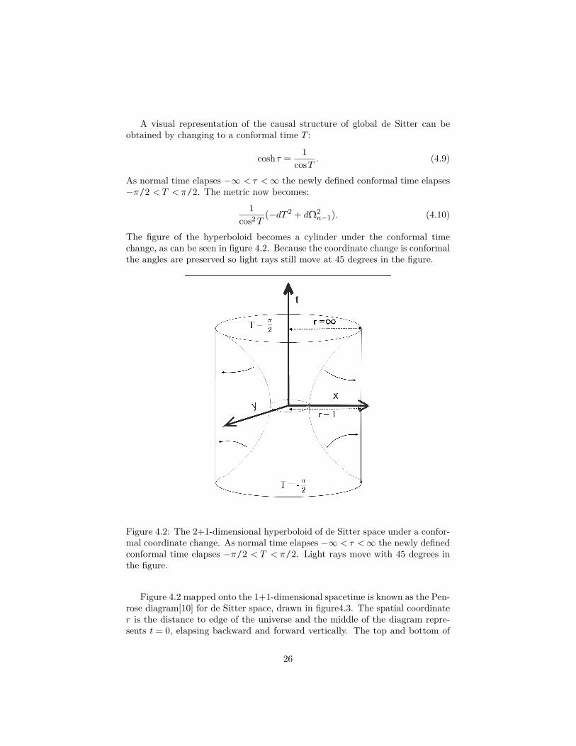
A visual representation of the causal structure of global de Sitter can beobtained by changing to a conformal time T :

coshτ = 1cosT . (4.9)

As normal time elapses −∞ < τ <∞ the newly defined conformal time elapses−π/2 < T < π/2. The metric now becomes:

1cos2T

(−dT 2 + dΩ2n−1). (4.10)

The figure of the hyperboloid becomes a cylinder under the conformal timechange, as can be seen in figure 4.2. Because the coordinate change is conformalthe angles are preserved so light rays still move at 45 degrees in the figure.

Figure 4.2: The 2+1-dimensional hyperboloid of de Sitter space under a confor-mal coordinate change. As normal time elapses −∞ < τ <∞ the newly definedconformal time elapses −π/2 < T < π/2. Light rays move with 45 degrees inthe figure.

Figure 4.2 mapped onto the 1+1-dimensional spacetime is known as the Pen-rose diagram[10] for de Sitter space, drawn in figure4.3. The spatial coordinater is the distance to edge of the universe and the middle of the diagram repre-sents t= 0, elapsing backward and forward vertically. The top and bottom of

26

the diagram represent the future and past lightlike infinity limit. Light rays arerepresented by 45 degree lines.

An observer in the first region can never go to the third and fourth regionbecause then he would have to exceed light speed. The first region represents ourobservable universe while the third represents a hypothetic unreachable inverseuniverse. An observer that entered region four can never go back to either ofthese universes. There are other coordinate systems that satisfy the coordinateequation for de Sitter space(4.1). The next coordinate system explored is theso called static coordinate system.

Figure 4.3: The Penrose diagram of de Sitter space. The spatial coordinater is the distance to the edge of the universe and the middle of the diagramrepresents t= 0, elapsing backward and forward vertically. The top and bottomof the diagram represent the future and past lightlike infinity limit. Light raysare represented by 45 degree lines.

4.2.2 Static coordinatesAnother coordinate system for de Sitter space is the static coordinate system.We have the substitutions:

X0 =√l2 − r2 sinhτ

Xi = rωi, i= 1, ...,n− 2

Xn−1 =√l2 − r2 coshτ . (4.11)

27

Using equation (4.4) the static coordinates satisfy the de Sitter space equa-tion (4.1):

−X20 +

n−1∑i=1

X2i = (1− r2)(cosh2 τ − sinh2 τ ) + r2

n−1∑i=1

ω2i−1 = 12. (4.12)

The metric can be obtained by computing the differentials:

dX20 = (1− r2)cosh2 τdτ2 +

r2

1− r2 sinh2 τdr2,

dX21 = (1− r2) sinh2 τdτ2 +

r2

1− r2 cosh2 τdr2,

n−1∑i=1

dXi =n−1∑i=1

ωidr2 + r2

n−1∑i=1

dω2i . (4.13)

The line element for static de Sitter space can be obtained:

ds2 =−(1− r2)dτ2 +1

1− r2 dr2 + r2

n−1∑i=1

dω2i . (4.14)

The metric in static coordinates is independent of τ so we say it has a time-like killing vector ∂

∂τ. This means that the metric remains invariant under time

translation τ → τ + a. This is the coordinate system as seen from a staticobserver. Hence, it is given the signature ’static’ coordinates. At the pointr = 1 the time differential dτ2 vanishes while the radial differential dr2 blowsup, creating a singularity. This singularity restrains the static coordinates ofaccounting for anything beyond the point r= 1.

Hence, static coordinates only represent the first region of the Penrose di-agram of de Sitter space, as shown in figure 4.4. This first region is thereforecalled the static patch of de Sitter space.

4.2.3 Planar coordinatesAnother coordinate system that satisfies the coordinate equation for de Sitterspace(4.1) is called planar coordinates:

X0 = sinhτ − 12xix

ie−τ ,

Xi = xie−τ , i= 1, ...,n− 2,

Xn−1 = coshτ − 12xix

ie−τ , (4.15)

(4.16)

28

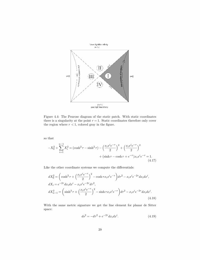
Figure 4.4: The Penrose diagram of the static patch. With static coordinatesthere is a singularity at the point r= 1. Static coordinates therefore only coverthe region where r < 1, colored gray in the figure.

so that

−X20 +

n−1∑i=1

X2i = (cosh2 τ − sinh2 τ )−

(xixie−τ2

)2+(xixie−τ

2

)2

+ (sinhτ − coshτ + e−τ )xixie−τ = 1.

(4.17)

Like the other coordinate systems we compute the differentials:

dX20 =

(cosh2 τ +

(xixie−τ2

)2− coshτxixie−τ

)dτ2 − xixie−2τdxidx

i,

dXi = e−2τdxidxi − xixie−2τdτ2,

dX2n−1 =

(sinh2 τ +

(xixie−τ2

)2− sinhτxixie−τ

)dτ2 − xixie−2τdxidx

i.

(4.18)

With the same metric signature we get the line element for planar de Sitterspace:

ds2 =−dτ2 + e−2τdxidxi. (4.19)

29

Instead of a timelike killing vector planar de Sitter space has a spacelike killingvector. As time elapses backwards to past infinity the spatial coordinates expandexponentially. The planar coordinates represent an expanding universe fromfuture to past infinity. It can be seen as the hyperboloid of de Sitter space, butsliced up at a 45 degree angle, shown in figure 4.5. Constructing the conformalPenrose diagram reveal that only the first and fourth region are covered byplanar coordinates.

Figure 4.5: The hyperboloid of de sitter space in planar coordinates. In planarcoordinates the universe expands exponentially from future to past infinity.There only the gray area is covered by planar coordinates

It is also possible to set up planar coordinates for an expansion forward intime covering the second and first region:

X0 = sinhτ − 12xix

ieτ ,

Xi = xieτ , i= 1, ...,n− 2,

Xn−1 = coshτ − 12xix

ieτ , (4.20)

ds2 =−dτ2 + e2τdxidxi. (4.21)

30

In figure 4.6 the diagram is shown for both future and past expanding planarcoordinates of de Sitter space.

Figure 4.6: The Penrose diagrams of the planar coordinates. The left diagramshows the planar coordinates representing a universe, exponentially expandingas time elapses backwards. Only the first and fourth region are covered by thesecoordinates, colored gray. The right diagram shows the planar coordinates fora future expanding universe. These coordinates only cover the first and secondregion of the Penrose diagram.

The goal of this chapter is to compare the in- and out-states of the total deSitter space, so the global coordinate system seems the right coordinate systemto work with.

However, there is one problem with this coordinate system. The spatial co-ordinates in this system increase with time. This is not the case for an earthlyobserver, in our perception length scales remain the same over time. This istherefore the system of some meta observer living in a system with only transla-tional symmetry. Nevertheless, the purpose of this thesis was to explore particlecreation in curved spacetime, not necessarily our spacetime. We will thereforeuse the global coordinate system for the computation of particle creation. Moreinformation about different coordinate systems of de Sitter space with referenceto the particle creation can be found in [11].

31

4.3 Transmission and reflection in global de Sit-ter space

In this section a start of the computation of the particle creation in de Sitterspace will be made following [12]. This will be done by computing the transmis-sion and reflection of a propagated scalar field from past to future infinity. Thestart of the problem will the same as the FRW computation. In n-dimensionalglobal coordinates the line element for de Sitter space is:

ds2 =−dτ2 + cosh2 τdΩ2n−1 , (4.22)

with dΩn−1 the metric of the hypersphere Sn−1 as in (4.5). For example in 2+1dimensions we have

dΩ2n−1 = dθ2 + sin2 θdφ2. (4.23)

From the definition of the line element ds2 = gµνdxµdxν the metric tensor gµν

for de Sitter space can be obtained. For example the metric tensor in 2+1-dimensions becomes:

gµν =

−1 0 00 cosh2 τ 00 0 sin2 θ cosh2 τ

, (4.24)

with determinant

det(g) =−sin2 θ(cosh2)2. (4.25)

To compute the transmission and reflection coefficients, we need the modes of ascalar field, propagated from the infinite past. The scalar field φ should satisfythe Klein-Gordon equation:

(−m2)φ= 0, . (4.26)

Here m is the mass of the total field. We choose m to be large because therewill be no particle creation without mass if the case is similar to FRW space.The next step is to determine the de Sitter Laplacian . This can be done withthe calculated metric tensor(4.24):

(τ ,θ,φ)≡ 1√−g

∂µ√−ggµν∂ν , (4.27)

=1

r2 sinθ cosh−2 τ∂µr2 sinθ cosh2 τgµν∂ν ,

=−cosh−2 τ∂τ [cosh2 τ∂τ ] + cosh−2(θ,φ), (4.28)

with (θ,φ) the spherical Laplacian of the 2 dimensional hypersphere. Extrap-olating this to n dimensions means we have to change (θ,φ) to the sphericalLaplacian of the n-1-dimensional hypersphere Sn−1. The hyperbolic cosines

32

should then be written with powers of n− 1. We get the de Sitter Laplacian inn dimensions:

=−cosh1−n τ∂τ [coshn−1 τ∂τ ] + cosh−2 τSn−1 . (4.29)

This enables us two write down the equation of motion in de Sitter space:

(−cosh1−n τ∂τ [coshn−1 τ∂τ ] + cosh−2 τSn−1 −m2)φ= 0. (4.30)

Like the computation for FRW space, we expand the field φ into modes:

φ=∑l

[a−l φl + a+l φ∗l ]. (4.31)

We are going to solve the equation of motion for each mode separately. It isconvenient to separate the spatial and time dependent part of the modes. Thespatial coordinates can be written as the normalized spherical harmonics on thehypersphere Sn−1. We can write:

φl = ul(τ )(coshτ )−n−1

2 Yl(Ωn−1). (4.32)

where the term cosh(τ )−n−1

2 is chosen for convenience of further computation.The spherical hamonics Yl(Ωn−1) are the eigenfunctions of the spherical Lapla-cian Sn−1 . The corresponding eigenvalues are[13]:

∆Sn−1Yl(Ωn−1) =−l(l+ n− 2)Yl(Ωn−1). (4.33)

The equation of motion (4.26) can be written:

−cosh1−n τ∂τ [cosh(τ )n−1∂τ ]u(τ )cosh(τ )1−n

2

− (l(l+ n− 2)cosh(τ )−2 +m2)u(τ )cosh(τ )1−n

2 = 0. (4.34)

By computing the first partial derivative with for notational convenience ∂τu(τ ) =u(τ ) and a= 1− n we have:

−cosha τ∂τ [u(τ )cosh(τ )−a2 + u(τ ) sinh(τ )a2 cosh(τ )−

a2−1]

−(l(l+ n− 2)cosh(τ )−2 +m2)u(τ )cosh(τ )a2 = 0. (4.35)

After evaluating the second partial derivative it looks like:

u(τ ) + u(τ )a

2 − u(τ )a(a+ 2)

4 +[a(a+ 2)

4 + l(l+ n− 2)]u(τ )cosh(τ )−2 +m2u(τ ) = 0.

(4.36)

By filling in a= 1− n the equation of motion for de Sitter space is obtained:[∂2τ +

2l+ n− 32

2l+ n− 12

1cosh2 τ

+ (m2 − (n− 1)2

4 )

]u(τ ) = 0. (4.37)

33

To create an idea what kind of equation we have encountered we make thesubstitutions:

L≡ 2l+ n− 12 , ω≡

√m2 − (n− 1)2

4 , (4.38)

so that: [− ∂2

τ −L(L− 1)cosh2 τ

]u(τ ) = ω2u(τ ). (4.39)

If the variable τ is viewed as a spatial variable, this equation is the ordinary onedimensional time-independent Schrödinger equation. The potential correspond-ing to this Schrödinger equation is known as the Poschl-Teller potential[14]:

V =−L(L− 1)cosh2 τ

. (4.40)

Notice that for odd dimensional de Sitter space the variable L becomes aninteger, and half integer for even dimensions. The difference between half integerand integer L has a drastic influence on the calculation of particle creation. Forthis thesis is chosen to stay restricted to the odd dimensional de Sitter spacewith integer L.

4.3.1 Direct solution of the Poschl-Teller wave equationIn this subsection the transmission and reflection coefficients for the solutionsof the Poschl-Teller Schrödinger equation will be computed. We refer to [15]for more information on solving the Poschl-Teller equation and other similarequation. The equation of motion with the Posch-Teller potential is:[

∂2τ + ω2 +

L(L− 1)cosh2 τ

]u= 0. (4.41)

At past and future infinity we can approximate

coshτ →∞, τ →±∞, (4.42)

so the equation of motion becomes

[∂2τ + ω2]u= 0. (4.43)

The solutions to this differential equation are

u=Ce±iω, τ →±∞ C ∈C. (4.44)

Therefore the modes should be of the following form to compute the reflectionand transmission of a from the infinite past propagated wave:

u= Teiωτ , τ →+∞eiωτ +Re−iωτ , τ →−∞. (4.45)

34

First we are going to define some substitution to simplify the equation of motion.After that the equation of motion, without the approximation, will be solved todetermine the exact modes. With the substitution y≡ cosh2 τ we have:

∂τ = ∂ydy

dτ= 2sinhτ coshτ∂y =

√−4(1− y)y∂y, (4.46)

∂τu= 2i√y(1− y)∂yu, (4.47)

∂2τu=−4y(1− y)∂2

yu− 2(1− 2y)∂yu. (4.48)

The differential equation becomes

[y(1− y)∂2y + (1/2− y)∂y −

ω2

4 −L(L− 1)

4y ]u= 0. (4.49)

By choosing u≡ yL/2v(y) the differentials can be rewritten

u≡ yL/2v(y), ∂yu= (L

2y v+ ∂yv)yL/2, (4.50)

∂2y = (L/2(L/2− 1)y−2v+ Ly−1∂yv+ ∂2

yv)yL/2, (4.51)

leading to the differential equation:

y(1− y)∂2yv+ ((L+ 1/2)− (L+ 1)y)∂yv− 1/4(L2 + ω2)v= 0. (4.52)

This is a hypergeometric equation[4] of the form

x(1− x)∂2xz + (c− (a+ b+ 1)x)∂xz − abz = 0, (4.53)

where

x= 1− y, z = v, (4.54)a= 1/2(L+ iω), b= 1/2(L− iω), c= 1/2, (4.55)

ab= 1/4(L2 + ω2). (4.56)

The solution to equation (4.52) is a linear combination of the hypergeometricfunctions:

v=A2F1(a,b, 12 ;1− y) +B

√1− y2F1(a+

12 ,b+ 1

2 , 32 ;1− y), (4.57)

where A and B are some constants. The constants A and B can be restrictedby setting up the scattering problem(4.45). First we change back to the originaltime variable cosh2 τ = y. Using the proposed substitution for u (4.50) we get:

u= v coshL τ ,

=AcoshL τ 2F1(a,b, 12 ;−sinh2 τ ),

−B coshL τ sinhτ 2F1(a+12 ,b+ 1

2 , 32 ;−sinh2 τ ). (4.58)

35

This function has an even and an odd part because of the respectively even andodd properties of the hyperbolic cosine and sine. The modes u can be rewritten

u=Aue(ven) +Buo(dd). (4.59)

For the calculation of the reflection and transmission between the far past en fu-ture only the infinitely large negative and positive values of τ matter. Thereforethe hyperbolic functions can be approximated:

sinha τ = (12 (e

τ − e−τ ))a→ (±1)a2−aea|τ |, for τ →±,∞ (4.60)

cosha τ = (12 (e

τ + e−τ ))a→ 2−aea|τ |, for τ →±.∞ (4.61)

The hypergeometric functions written in terms of gamma functions [15] become:

ue(τ )→ 2−LeL|τ |Γ(12 )(

Γ(b− a)Γ(b)Γ( 1

2 − a)22ae−2a|τ |

+Γ(a− b)

Γ(a)Γ( 12 − b)

22be−2b|τ |)

, (4.62)

uo(τ )→ ± 2−(L+1)e(L+1)|τ |Γ(32 )(

Γ(b− a)Γ(b+ 1

2 )Γ(1− a)22a+1e−(2a+1)|τ |

+Γ(a− b)

Γ(a+ 12 )Γ(1− b)

22b+1e−(2b+1)|τ |)

, τ →±∞. (4.63)

The ± sign in the odd solution is used respectively for τ being in the infinitepast and future limit. By filling in the variables a and b (4.55) we get:

ue(τ )→ Γ(12 )(Ee

−iω|τ | +E∗eiω|τ |), (4.64)

uo(τ )→±Γ(32 )(Oe

−iω|τ | +O∗eiω|τ |), (4.65)

where

E ≡ Γ(−iω)Γ(L2 −

iw2 )Γ( 1−L

2 − iw2 )

eiω log2, (4.66)

O≡ Γ(−iω)Γ(L+1

2 − iw2 )Γ(1− L

2 −iw2 )

eiω log2. (4.67)

We have found the mode solutions for the time dependent part of the deSitter equation of motion. We are now going to proceed different from the FRWapproach by setting up the scattering problem. The total solution is the linearcombination of the odd and even solutions:

u=A(Eeiωτ +E∗e−iωτ )−B(Oeiωτ +O∗e−iωτ ),τ →−∞A(Ee−iωτ +E∗eiωτ ) +B(Oe−iωτ +O∗eiωτ ),τ →∞

. (4.68)

36

As mentioned before the past and future infinity limit of the modes should beof the form:

u= Teiωτ , τ →+∞.eiωτ +Re−iωτ , τ →−∞,

. (4.69)

The purpose of the following computation will be to determine the reflectionand transmission coefficients R and T . The scattering set up defines restrictionon the constants A and B by

AE +BO= 0, (4.70)AE −BO= 1, (4.71)

so that the transmission and reflection coefficients become:

T =AE∗ +BO∗, (4.72)R=AE∗ −BE∗. (4.73)

It can be assumed that E and O are functions of some arguments φe/o. Thesearguments can be defined to be real by allocating real factors Ce and Co to thesolutions:

E =Ceeiφe , O=Coe

iφo , (4.74)

where

φe,φo,Ce,Co ∈R. (4.75)

By equating (4.70) and (4.71) we will get

ACe =12e−iφe , BCo =

12e−iφo . (4.76)

Hence, the equations for the reflection and transmission coefficients can berewritten:

T =12 (e−2iφe − e−2iφo), (4.77)

R=12 (e−2iφe + e−2iφo). (4.78)

For the calculation of the transmission and reflection the exponentials e−iφe ande−iφo need to be calculated. From equations (4.66) and (4.67) one obtains:

Cee−iφe =E∗ =

Γ(iω)Γ(L2 + iw

2 )Γ( 1−L2 + iw

2 )e−iω log2, (4.79)

Cee−iφo =O∗ =

Γ(iω)Γ(L+1

2 + iw2 )Γ(1− L

2 + iw2 )

e−iω log2. (4.80)

37

Now using the fact that |E|=Ce the even exponential can be written:

e−2iφe =E∗2

C2e

=E∗2

|E∗|2=E∗

E

= ei2φe = e2iω log2 Γ(iω)Γ(L2 −iω2 )Γ( 1−L

2 − iω2 )

Γ(−iω)Γ(L2 + iω2 )Γ( 1−L

2 + iω2 )

. (4.81)

The same applies to the odd solution:

e−2iφo =O∗2

C2o

=O∗2

|O∗|2=O∗

O

= e−2iω log2 Γ(iω)Γ(L+12 − iω

2 )Γ(1− L2 −

iω2 )

Γ(−iω)Γ(L+12 + iω

2 )Γ(1− L2 + iω

2 ). (4.82)

Starting with the odd solution the arguments of the Gamma functions are sub-stituted

Z1 ≡L+ 1

2 − iω

2 , (4.83)

so that

e−2iφo = e−2iω log2 Γ(iω)Γ(Z1)Γ( 32 −Z

∗1 )

Γ(−iω)Γ(Z∗1 )Γ(32 −Z1)

. (4.84)

By multiplying with

Γ(1−Z∗1 )Γ(1−Z1)

Γ(1−Z∗1 )Γ(1−Z1), (4.85)

the gamma functions can be simplified. We can use the properties of gammafunctions[4]:

Γ(Z)Γ(1−Z) = π

sin(πZ) , (4.86)

Γ(Z)Γ(Z +12 ) = 21−2Z√πΓ(2Z). (4.87)

The exponential takes the form

e−2iφo = e−2iω log2 Γ(iω)π sin(πZ∗1 )22Z∗1−1√πΓ(2− 2Z∗1 )Γ(−iω)π sin(πZ1)22Z1−1√πΓ(2− 2Z1)

. (4.88)

We can put back Z1 =L+1

2 − iω2 :

e−2iφo = e−2iω log2 Γ(iω) sin(πL+12 + π iω2 )2L+iωΓ(1−L− iω)

Γ(−iω) sin(πL+12 − π iω2 )2L−iωΓ(1−L+ iω)

. (4.89)

38

Using the fact that L is an integer, the sines can be simplified to

sin(πL+12 + π iω2 )

sin(πL+12 − π iω2 )

=cos(πL2 )cosh(π iω2 )− isin(πL2 ) sinh(π iω2 )

cos(πL2 )cosh(π iω2 ) + isin(πL2 ) sinh(π iω2 )= (−1)L.

(4.90)

Because L is also a positive integer, the gamma functions can be simplified usingthe formula

Γ(z − n) =n∏l=1

(z − l)−1Γ(z). (4.91)

Both equations (4.90) and (4.91) do not hold for half integer values of L. This isthe reason why the particle creation is differently in even-dimensional de Sitterspace. Now the exponential will be maximally simplified:

e−2iφo = (−1)L

L−1∏n=1

(iω− n)

L−1∏n=1

(−iω− n)

=−

L−1∏n=1

(−iω+ n)

L−1∏n=1

(−iω− n)=−

L−1∏n=1

ω+ in

ω− in. (4.92)

The same can be done for the even solution:

Z2 ≡L

2 −iω

2 , (4.93)

e−i2φe = e−2iω log2 Γ(iω)π sin(πZ∗2 )22Z∗2√πΓ(1− 2Z∗2 )

Γ(−iω)π sin(πZ2)22Z2√πΓ(1− 2Z2)

(4.94)

= (−1)L−1

L−1∏n=1

(iω− n)

L−1∏n=1

(−iω− n)(4.95)

=

L−1∏n=1

(−iω+ n)

L−1∏n=1

(−iω− n)=L−1∏n=1

ω+ in

ω− in. (4.96)

Following equation (4.77) the transmission and reflection coefficients can be

39

computed with these exponentials. The transmission becomes:

T =12 (e−2iφe − e−2iφo)

=12 (L−1∏n=1

ω+ in

ω− in+L−1∏n=1

ω+ in

ω− in) (4.97)

=L−1∏n=1

ω+ in

ω− in, (4.98)

and the reflection:

R=12 (e

2iφe + e2iφo)

=12 (L−1∏n=1

ω+ in

ω− in−L−1∏n=1

ω+ in

ω− in) = 0. (4.99)

Thus, we have shown that odd dimensional de Sitter space has a reflectionlesspotential. Before relating this to the Bogoliubov coefficients the phenomenon ofreflectionless potentials will be further explored. This will be done in the nextsubsection with algebraic means.

4.3.2 Approaching reflectionless potentials algebraicallyIn the previous subsection we have encountered the phenomenon of reflection-less potentials. This is a property that normally would only be expected for anequation of motion with a constant potential. This is obviously not the case forthe wave function in the de Sitter space(4.37). In this subsection the basic con-cept of reflectionless potentials is explored following[12]. An algebraic methodis used to construct arbitrary reflectionless potentials. As will be shown thisleads quite straightforward to the potential found for the de Sitter space. Westart with an arbitrary Hamiltonian of the form:

H(τ ) = p2 + V (τ ), (4.100)

where p=−i∂τ and V (τ ) approaches a constant in the past and future infinitylimit: τ →±∞. The Hamiltonian can be rewritten in terms of ladder operatorsA+ and A−. To prevent confusion, these are ladder operators arbitrarily chosenand have nothing to do with the ladder operators of the mode solutions. Thereare two ways of combining these ladder operators so we can create two differentHamiltonians defined H+ and H−:

H+ ≡A+A−, H− ≡A−A+. (4.101)

The ladder operators are defined:

A± ≡ p± iW (τ ), (4.102)

40

withW (τ ) some potential that becomes a constant in the past and future infinitylimit. Now substituting the ladder operators we get for the hamiltonians:

H± = (p± iW (τ )(p∓ iW (τ ))

= p2 +W (τ )2 ∓ piW (τ )± iW (τ )

= p2 +W (τ )2 ∓ ∂τ [W (τ )]. (4.103)

As both H+ and H− should be of the form (4.100) we can define a pair for thepotentials in the same way:

V± ≡W 2 ∓ ∂τ [W (τ )]. (4.104)

Just likeW (τ ) will V± approach a constant in the past and future infinity limit.We can write:

H± |ψ±〉=E± |ψ±〉 . (4.105)

where |ψ±〉 and E± are an eigenstate and corresponding energy of the Hamilto-nian H±. The eigenstate |ψ±〉 can be converted to an eigenstate of the Hamil-tonian H∓ by letting the operator A∓ act on it:

H∓[A∓ |ψ±〉] =A∓A±A∓ |ψ±〉=A∓H± |ψ±〉=A∓E± |ψ±〉=E±[A∓ |ψ±〉].(4.106)

We can set up the problem for the computation of the reflection and transmissionthe same way as before but now for the + and − states independently:

ψ± = T±eiωτ , τ →+∞eiωτ +R±e−iωτ , τ →−∞

. (4.107)

The two Hamiltonians will have different transmission and reflection coefficientsbecause their eigenstates differ. As stated before the eigenstates of H+ can beconverted to the eigenstates of H− so that:

aψ− =A−ψ+, (4.108)

with a the eigenvalue of A− acting on ψ. Filling in A− and ψ± we get for thefar past limit:

a(eiωτ +R−e−iωτ ) = (p− iW (−∞))(eiωτ +R+e

−iωτ )

= ωeiωτ − iW (−∞)eiωτ −R+ωe−iωτ − iW (−∞)R+e

−iωτ

= [ω− iW (−∞)]eiωτ − [ω+ iW (−∞)]R+e−iωτ . (4.109)

No limitations have been given on the eigenvalue a so we can choose a = ω −iW (−∞). Now the terms with eiωτ cancel, leaving

R− =ω+ iW (−∞)

−ω+ iW (−∞)R+. (4.110)

41

The same can be done in the far future limit:

aψ− =(ω− iW (−∞))T−eiωτ = (p− iW (∞)T+e

iωτ , (4.111)

⇒ T− =ω− iW (∞)

ω− iW (−∞)T+. (4.112)

From equation (4.110) we can conclude that if the reflection coefficient R− isequal to zero, the reflection coefficient R+ must be zero too. If we can constructa potential V− that has no reflection we know that the partner potential V+ willalso be reflectionless. A wavefunction with a constant potential at any time τwill have no reflection so we can choose the reflectionless potential:

V− =W (τ )2 + ∂τ (W (τ )) = 1. (4.113)

This differential equation has the solution

W (τ ) = tanhτ . (4.114)

From here the partner potential V+ can be computed:

V+ =W (τ )2 − ∂τ (W (τ ) = 1− 2cosh2 τ

. (4.115)

A shift of the potential will not affect the reflectionless property so the constantterm can be neglected. Now we can choose V+ to be the lower potential of somenew potential, say V2, in the exact same way as V− is the lower potential of V+.We will get a new differential equation for a new W2(τ ):

W2(τ ) + ∂(W2(τ )) =2

cosh2 τ. (4.116)

By adding a constant that will not affect the reflectionless property this differ-ential equation has a straightforward solution:

W2(τ ) + ∂(W2(τ )) = 4− 2cosh2 τ

, (4.117)

⇒W2(τ ) = 2tanhτ . (4.118)

The new potential V2 can be calculated which by equation (4.110) will also bereflectionless:

W 22 (τ )− ∂(W2(τ )) = 4− 6

cosh2 τ. (4.119)

This procedure can be repeated an infinitely many times and every new foundpotential will be reflectionless. Take notice that V2, neglecting the constant, isthe potential corresponding to the second repetition of this procedure and canbe written:

V2 =−M (M + 1)

cosh2 τ, M = 2. (4.120)

42

Assuming this is the case for any arbitrary M ∈Z we have

VM =−M (M + 1)cosh2 τ

(4.121)

WM+1(τ )+∂(WM+1(τ )) = (M + 1)2 − M(M + 1)cosh2 τ

(4.122)

⇒WM+1(τ ) = (M + 1) tanhτ . (4.123)

The new potential can be computed:

WM+1(τ )− ∂τ (WM+1(τ )) = (M + 1)2 − (M + 1)2 + (M + 1)cosh2 τ

. (4.124)

This proofs that for any integer M ∈Z the potential VM =−M(M+1)cosh2 τ

is reflec-tionless. Even the defined lowest order potential V− can be written in terms ofthis potential by choosing M = 0. The transmission coeffient can be computedfrom (4.112) together with (4.123):

TM =ω− iWM (−∞)

ω− iWM (∞)TM − 1 = ω− iM tanh(−∞)

ω− iM tanh(∞)TM

=ω+ iM

ω− iM. (4.125)

T0 is defined to be equal to one so the transmission becomes:

T =M∏n=1

ω+ in

ω− in. (4.126)

Choosing M to be L− 1 we get the potential found for the de Sitter space withthe same transmission coefficient computed before.

V =−L(L− 1)cosh2 τ

, (4.127)

T =L−1∏n=1

ω+ in

ω− in. (4.128)

This confirms that odd dimensional de Sitter space has a reflectionless potential.

4.4 Particle creation in de Sitter spaceIn this section the final step towards particle creation in de Sitter space will bemade. The reflectionless property of the Poschl-Teller potential has an inter-esting consequence for the particle creation. To determine the particle creationwe first need to establish the relation between the transmission and reflectionand the Bogoliubov coefficients. More on this relation is found in [16].With

43

the reflection and transmission coefficients we can write exact solutions to theKlein-Gordon equation at the infinite past and future limit. The first thing todo is changing back to the original modes(4.32):

φl = u(τ )Yl(Ωn−1)cosh−n−1

2 τ . (4.129)

Following the problem for the reflection and transmission coefficients (4.45)wecan write:

φl = Yl(Ωn−1)cosh−n−1

2 τTeiωτ , τ →+∞Yl(Ωn−1)cosh−

n−12 τ (eiωτ +Re−iωτ ) τ →−∞,. (4.130)

Just like with the FRW spacetime we can obtain the Bogoliubov coefficientsby writing the in-state, where τ →−∞, as a linear combination of out-states,where τ →∞:

φinl = αlluoutl + βl−lu

out∗−l . (4.131)

By noticing that the hyperbolic cosine is real and an even function so thatcoshτ = cosh−τ this can be done in the current form:

φinl = Yl(Ωn−1)cosh−n−1

2 τ (eiωτ +Re−iωτ )

= Yl(Ωn−1)cosh−n−1

2 τ (1TTeiωτ +

R

TTe−iωτ

=1Tφoutl +

R

Tφout∗l . (4.132)

Hence, the Bogoliubov coefficients in global de Sitter space are given:

|βk|2 =|R|2

|T |2, (4.133)

|αk|2 =1|T |2

. (4.134)

In this case the reflection coefficient is equal to zero, therefore the second Bo-goliubov coefficient is also zero. The expectation value of the number operatoris related to the absolute squared value of the second Bogoliubov coefficient:

Nk = |βk|2. (4.135)

The de Sitter universe in odd dimensions with no particles at the infinite past,the vacuum in-state, will have no particles at the infinite future. However, thiscomputation does not give information about particle creation in between theinfinities. It could be possible that particles are created and then annihilatedsomewhere between the past and future infinity limit[11]. As we are not living inthe past or future infinity limit, this is another reason why our universe cannotbe described by this computation. Up till now we have been restricted to deSitter space in odd dimension. In the next section will be discussed in which waythe computation of the particle creation for de Sitter space in even dimensionsspace differs from odd dimensions.

44

4.5 De Sitter space in even dimensionsThis section will discuss the particle creation for de Sitter space in even di-mensions. It is not necessary to set up the whole problem from the start tocompute the particle creation. Most of the computation done in section 4.3.1is the same for the even-dimensional case. Instead of redoing the computationonly the differences will be discussed and the influence on the particle creation.

For odd dimensions the variable L in the equation of motion is an integer(4.38) while for even dimensions L becomes a half integer. For half integervalues of L the algebraic method used in section 4.3.2 will get no results. Thereflectionless potential derived in that section looked like

VM =C − M (M + 1)cosh2 τ

, (4.136)

with C some constant that did not affect the reflectionless property. The lowestorder potential for integer M was defined to be a reflectionless potential bychoosing M = 0:

V− = (0 + 1)2 − 0(0 + 1)cosh2 τ

= 1. (4.137)

However, now we have half integers for M so the lowest value can not be chosenequal to zero. The lowest positive value will now be M = 1/2 so that

V− = (1/2)2 − 1/2(1/2 + 1)cosh2 τ

= (1/4)− 34cosh2 τ

. (4.138)

For any half integer value of M there will a term with cosh−2 τ , leading to acomparable differential equation as the equation we started with (4.41). Hence,the only way to find out if the potential is reflectionless for even dimensions isby computing the equation of motion directly. For odd dimensions this is donein section 4.3.1.

We will now discuss where the direct solutions to the equation of motion forde Sitter space differ in even and odd dimensions. In section 4.3.1 there are twoequations that exploit the odd-dimensional property. The first equation is thesimplification of the sines (4.90). This equation cannot be used anymore whenL is a half integer. The second equation is the simplification of the gammafunctions (4.91). When L is a half integer the gamma functions can only bepartially simplified using

Γ(1−L∓ iω) = Γ(∓iω+ 1/2)L− 1

2∏n=1

(z − n)−1. (4.139)

45

Now using the same algebra as with the odd solution we will get the transmissionand reflection coefficients:

T =12

( sin(πL2 + π iω2 )

sin(πL2 − πiω2 )−

sin(πL+12 + π iω2 )

sin(πL+12 − π iω2 )

)Γ(iω)Γ(−iω− 1

2 )

Γ(−iω)Γ(iω− 12 )

L− 12∏

n=1

ω+ in

ω− in

= (−1)2L+1itanh(πω)Γ(iω)Γ(−iω− 1

2 )

Γ(−iω)Γ(iω− 12 )

L− 12∏

n=1

ω+ in

ω− in, (4.140)

R=12

( sin(πL2 + π iω2 )

sin(πL2 − πiω2 )

+sin(πL+1

2 + π iω2 )

sin(πL+12 − π iω2 )

)Γ(iω)Γ(−iω− 1

2 )

Γ(−iω)Γ(iω− 12 )

L− 12∏

n=1

ω+ in

ω− in

=1

coshπωΓ(iω)Γ(−iω− 1

2 )

Γ(−iω)Γ(iω− 12 )

L− 12∏

n=1

ω+ in

ω− in. (4.141)

The scattering coefficients found for even dimensions cannot be as easily simpli-fied as the coefficients for odd dimensions. However, following (4.133) we needthe absolute squared values of the coefficients to compute the particle creation.We can write:

|T |2 = T ∗T = tanh2(πω), (4.142)

|R|2 =R∗R=1

coshπω . (4.143)

Now using equation (4.133) and (4.135) we will get the particle creation for deSitter space in even dimensions:

Nk = |βk|2 =|R|2

|T |2=

1sinh2πω

(4.144)

We put back the frequencys in terms of the field mass (4.38):

Nk =1

sinh2π√m2 − (n−1)2

4

. (4.145)

Notice that this expression becomes complicated when the mass m of the fieldis low. When m2 < (n−1)2

4 the particle creation becomes imaginary and theperiodic sine would blow up. These complications can be avoided by keepingrestricted to a massive field.

In summary, de Sitter space in global coordinates with even dimensions hasno particle creation between past and future infinity. However, when changingto even dimensions this is not the case for a massive field and particles arecreated.

46

Chapter 5

Conclusion and discussion

It has been shown that particle production is a property of curved spacetime.The particle production is directly connected to the coefficients of the Bo-goliubov transform. With this we tried to compute the particle creation inFriedmann-Robertson-Walker space and de Sitter space. This is done by com-paring the infinite past with the infinite future limit.

We started with Friedmann-Robertson-Walker space, the conformally flatspacetime model describing a smoothly expanding universe. The result was anon-zero value for the Bogoliubov coefficients for a massive field. The conclusioncould therefore be made that curved spacetime indeed leads to particle produc-tion. This is a very interesting property, meaning that a smoothly expandingmassive universe starting out as empty vacuum in the far past will have particlesat the far future.

The next explored spacetime model was odd dimensional de Sitter space, de-scribing an accelerated expanding universe. There are many ways of putting upcoordinate systems satisfying the definition of de Sitter space. In this thesis wehave restricted us to the coordinate system covering the whole of de Sitter space,so called global coordinates. The whole of de Sitter space can be described by ahyperboloid: Infinite expansion at the far past and future limit and its minimumat the present. It became clear that odd and even dimensions made a great dif-ference to the computation of particle creation. The computation was done bysetting up a scattering problem of a propagated wave from past to future infinity.

It was found that there was no reflection of the propagated wave in odd-dimensional global de Sitter. This has been explored further by approachingarbitrary Hamiltonians with reflectionless potentials algebraically. This led tothe the same differential equation found for de Sitter space. We explored the di-rect relation between the scattering coefficients and the Bogoliubov coefficients.The conclusion was made that a vacuum state at past infinity will still be in thevacuum state at future infinity in odd dimensional global de Sitter space. After

47

that the differences between de Sitter space in even and odd dimensions were ex-plored. This led to the conclusion that, in contrast to odd-dimensional de Sitterspace, there is particle creation in massive de Sitter space with even dimensions.

In summary, there has been shown that curved spacetime can lead to particlecreation. However, not every curved spacetime model will necessarily lead toparticle creation. There is particle creation in massive Friedmann-Robertson-Walker space but in odd dimensional de Sitter space, when only looking at pastand future infinity, there is not.

This is not the last thing to be said about particle creation. There are manyother curved spacetime models that cause particle creation. The direct next stepwould be to explore the other coordinate systems of de Sitter space. For exam-ple the static coordinates could be described as the system of a static earthlyobserver. It then might be possible to try and describe astronomical observa-tions with the theory of particle production. As mentioned in the introductionthe inflationary period was approximately de Sitter, so particle creation shouldhave greatly influenced the early development of our observable universe.

48

Bibliography

[1] A. H. Guth, The Infralionary Universe: The Quest For a New Theory ofCosmic Origins. Helix Books, 1997.

[2] D. Tong, “Lectures on quantum field theory,” 2012. [Online]. Available:http://www.damtp.cam.ac.uk/user/tong/qft.html

[3] L. H. Ryder, Quantum Field Theory, 2nd ed. Cambridge university press,1996.

[4] E. Weisstein, “Wolfram mathworld,” 2014. [Online]. Available:http://mathworld.wolfram.com/

[5] N. Birrell and P. Davies, Quantum Fields in Curved Space, 1982.

[6] V. F. Mukhanov and S. Winitzki, Introduction to Quantum Fields in Clas-sical Backgrounds. Munich, Germany: Department of Physics, Ludwig-Maximilians University, 2004.

[7] S. Weinberg, Gravitation and cosmology: Principles and applications of thegeneral theory of relativity. John Wiley and Sons, Inc., 1972.

[8] I. S. Gradshteyn and I. M. Ryzhik, Table of Integrals, series and products,5th ed. Elsevier Inc., 2007.

[9] M. Spradlin, A. Strominger, and A. Volovich, “Les Houches lectures on deSitter space,” pp. 423–453, 2001.

[10] L. Susskind, “General relativity lectures,” 2012. [Online]. Available:https://continuingstudies.stanford.edu/

[11] G. Gibbons and S. Hawking, “Cosmological Event Horizons, Thermody-namics, and Particle Creation,” Phys.Rev., vol. D15, pp. 2738–2751, 1977.

[12] P. Lagogiannis, A. Maloney, and Y. Wang, “Odd-dimensional de SitterSpace is Transparent,” 2011.

[13] C. R. Frye and C. J. Efthimiou, “Spherical Harmonics in p Dimensions,”2012.

49

[14] G. Poschl and E. Teller, “Bemerkungen zur Quantenmechanik des anhar-monischen Oszillators,” Z.Phys., vol. 83, pp. 143–151, 1933.

[15] S. Flugge, Classics in mathematics, Practical Quantum Mechanics.Springer, 1994.

[16] R. Brout, S. Massar, R. Parentani, and P. Spindel, “A Primer for blackhole quantum physics,” Phys.Rept., vol. 260, pp. 329–454, 1995.

50