particle swarm optimization - nit srinagar

Particle Swarm optimization

Contents

Introduction to Optimization

Particle Swarm Optimization

Illustration of Algorithm

Mathematical Interpretation

Example

Dataset Illustration


The optimization can be defined as a mechanism through which the maximum or minimum value of a

given function or process can be found.

The function that we try to minimize or maximize is called as objective function.

Variable and parameters.

Statement of optimization problem

Minimize f(x)

subject to g(x)<=0

h(x)=0.

Two main phases Exploration and Exploitation


Application to optimization: Particle Swarm Optimization

Proposed by James Kennedy & Russell Eberhart (1995)

Combines self-experiences with social experiences

Particle Swarm Optimization(PSO)

Inspired from the nature social behavior and dynamic movements with communications of insects,

birds and fish.

Particle Swarm Optimization(PSO)

Uses a number of agents (particles) that constitute a

swarm moving around in the search space looking for the

best solution

Each particle in search space adjusts its “flying” according to its

own flying experience as well as the flying experience of other

particles.

Each particle has three parameters position, velocity, and previous

best position, particle with best fitness value is called as global best

position.

Contd..

Collection of flying particles (swarm) - Changing solutions

Search area - Possible solutions

Movement towards a promising area to get the global optimum.

Each particle adjusts its travelling speed dynamically corresponding to the flying

experiences of itself and its colleagues.

Each particle keeps track:

its best solution, personal best, pbest.

the best value of any particle, global best, gbest.

Each particle modifies its position according to:

• its current position

• its current velocity

• the distance between its current position and pbest.

• the distance between its current position and gbest.

Algorithm - Parameters

f : Objective function

Xi: Position of the particle or agent.

Vi: Velocity of the particle or agent.

A: Population of agents.

W: Inertia weight.

C1: cognitive constant.

R1, R2: random numbers.

C2: social constant.

Algorithm - Steps

1. Create a ‘population’ of agents (particles) uniformly distributed over X

2. Evaluate each particle’s position according to the objective function( say

y=f(x)= -x^2+5x+20

1. If a particle’s current position is better than its previous best position, update it.

2. Determine the best particle (according to the particle’s previous best positions).

Y=F(x) = -x^2+5x+20

Contd..

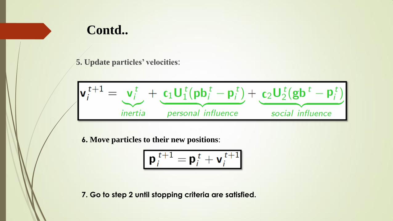
5. Update particles’ velocities:

6. Move particles to their new positions:

7. Go to step 2 until stopping criteria are satisfied.

Contd…

Particle’s velocity:

1. Inertia

2. Personal

Influence

3. Social

Influence

• Makes the particle move in the same direction and with the same velocity

• Improves the individual• Makes the particle return to a previous position,

better than the current• Conservative

• Makes the particle follow the best neighbors direction

Acceleration coefficients

• When , c1=c2=0 then all particles continue flying at their current speed until they hit the search space’s boundary.

Therefore, the velocity update equation is calculated as:

t

ij

t

ij vv 1

• When c1>0 and c2=0 , all particles are independent. The velocity update equation will be:

t

ijibesttt

j

t

ij

t

ij xPrcvv

,1

11

• When c1>0 and c2=0 , all particles are attracted to a single point in the entire swarm and

the update velocity will become

t

ijbest

t

j

t

ij

t

ij xgrcvv

221

• When c1=c2, all particles are attracted towards the average of pbest and gbest.

Contd…

Intensification: explores the previous solutions, finds the best solution of a

given region

Diversification: searches new solutions, finds the regions with potentially the

best solutions

In PSO:

Example:

Contd..

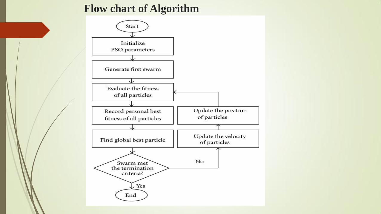
Flow chart of Algorithm

Mathematical Example and Interpretation

Fitness Function

De Jong Function

minF(x,y) = x^2+y^2

Where x and y are the dimensions of the problem. The surface and contour plot of the De Jong

function is given as:


Contd..

Rastrigin Function

The surface and contour plot of the De Jong function is given as:

)..2cos(.10(1 i

D

t i xx


Contd…

Banana Function

The surface and contour plot of the Rosenbrock function or 2nd De Jong function

Or valley or banana functions given as:


Example 1

Find the minimum of the function

205)( 2 xxxf

Using PSO algorithm. Use 9 particles with initial positions

10,3.8,8.2,3.2,6.0

,1.1,6.2,6,6.9

98765

4321

xxxxx

xxxx

Solution Choose the number of particles

10,3.8,8.2,3.2,6.0

,1.1,6.2,6,6.9

98765

4321

xxxxx

xxxx

Evaluate the objective function

30,39.7,16.26

,21.26,64.22,29.13

24.0,46,16.120

0

9

0

8

0

7

0

6

0

5

0

4

0

3

0

2

0

1

fff

fff

fff


Contd..

Let c1=c2=1 and set initial velocities of the particles to zero.

0,,,00

9

0

8

0

7

0

6

0

5

0

4

0

3

0

2

0

1

0

1 vvvvvvvvvv

Step2. Set the iteration no as t=0+1 and go to step 3

.

Step 3. Find the personal best for each particle by

So

10,3.8,8.2

3.2,6.0,1.1

6.2,6,6.9

9,1

8,1

7,1

6,1

5,1

4,1

3,1

2,1

1,1

bestbestbest

bestbestbest

bestbestbest

PPP

PPP

PPP


Contd..

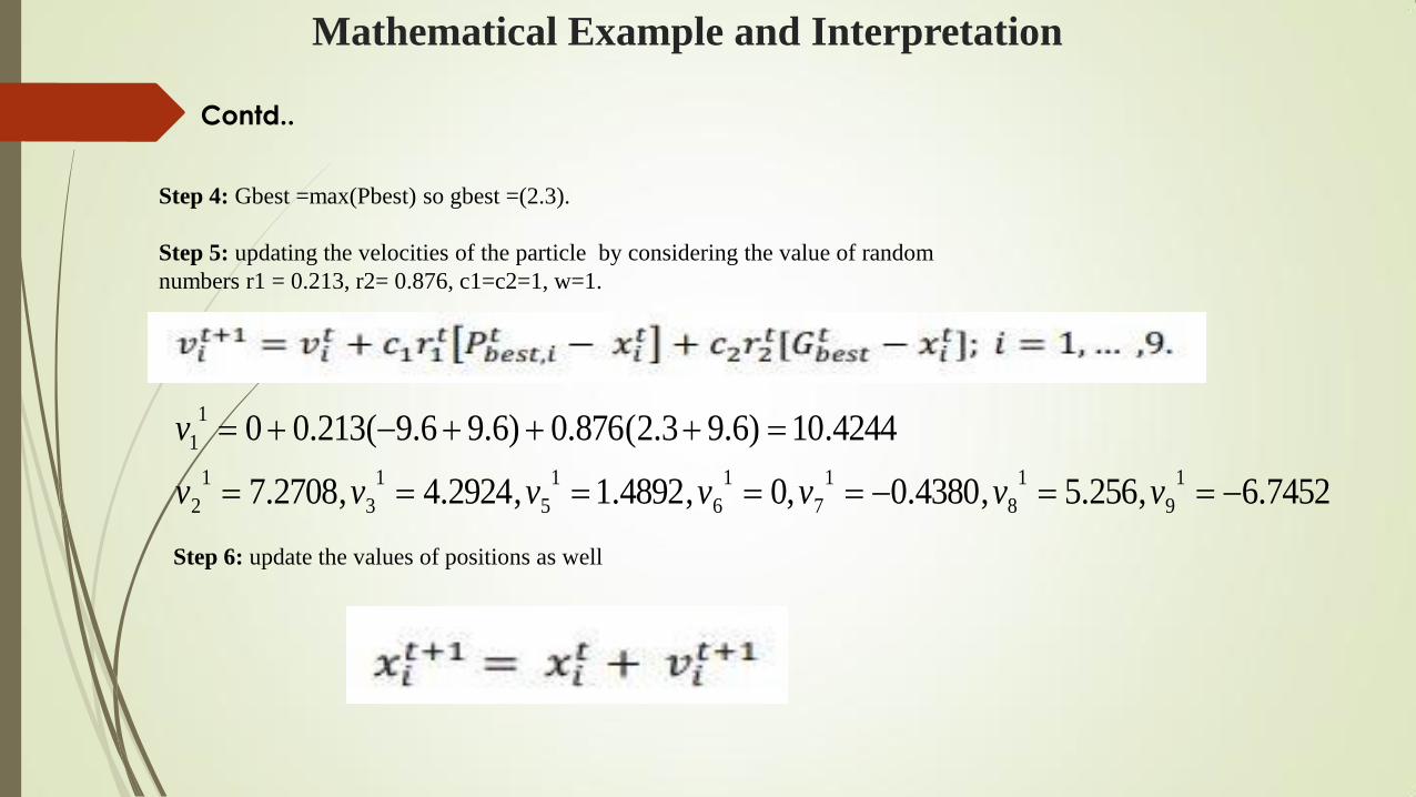
Step 4: Gbest =max(Pbest) so gbest =(2.3).

Step 5: updating the velocities of the particle by considering the value of random

numbers r1 = 0.213, r2= 0.876, c1=c2=1, w=1.

7452.6,256.5,4380.0,0,4892.1,2924.4,2708.7

4244.10)6.93.2(876.0)6.96.9(213.00

1

9

1

8

1

7

1

6

1

5

1

3

1

2

1

1

vvvvvvv

v

Step 6: update the values of positions as well


Contd..

So

2548.3,044.3,362.2

3.2,0892.2,8784.1

6924.1,2708.1,8244.0

1

9

1

8

1

7

1

6

1

5

1

4

1

3

1

2

1

1

xxx

xxx

xxx

Step7: Find the objective function values of

6803.25,9541.25,231.26

21.26,0812.26,8636.25

5978.25,739.24,4424.23

1

9

1

8

1

7

1

6

1

5

1

4

1

3

1

2

1

1

fff

fff

fff

Step 8: Stopping criteria

if the terminal rule is satisfied , go to step 2.

Otherwise stop the iteration and output the results.

Contd..

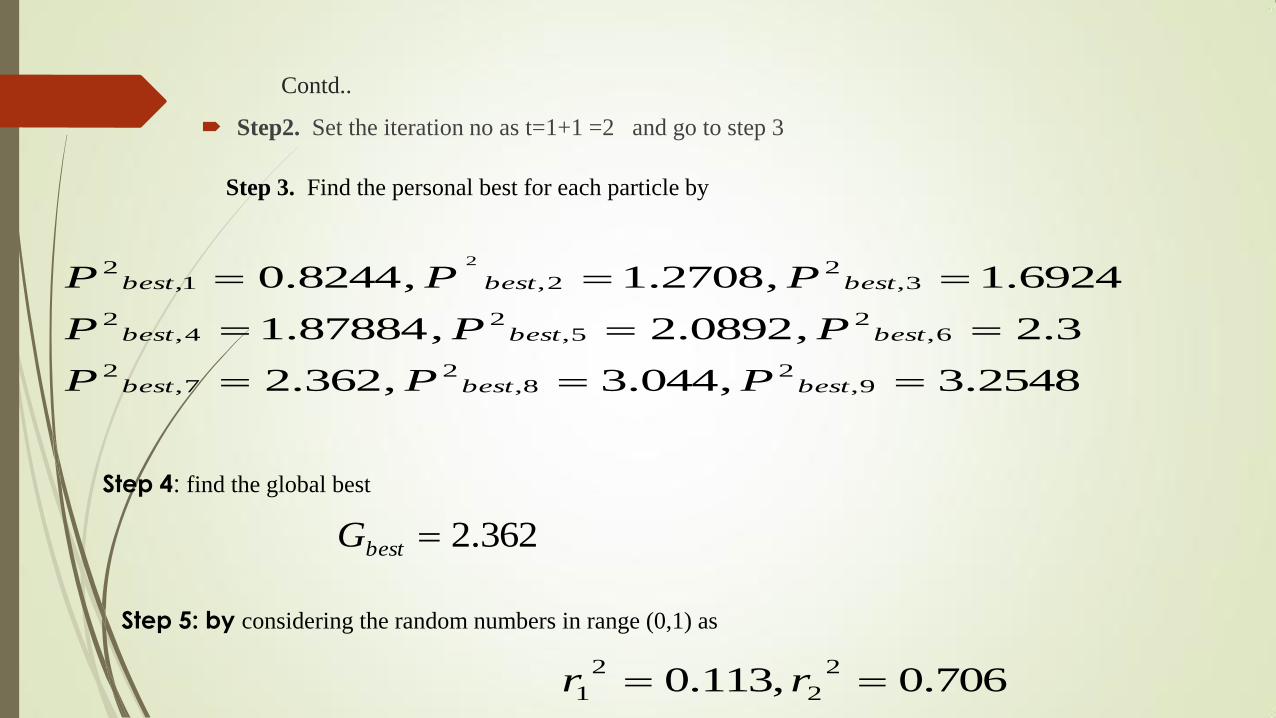
Step2. Set the iteration no as t=1+1 =2 and go to step 3


2548.3,044.3,362.2

3.2,0892.2,87884.1

6924.1,2708.1,8244.0

9,2

8,2

7,2

6,2

5,2

4,2

3,2

2,1,2 2

bestbestbest

bestbestbest

bestbestbest

PPP

PPP

PPP

Step 4: find the global best

362.2bestG

Step 5: by considering the random numbers in range (0,1) as

706.0,113.02

2

2

1 rr

Contd..

Find the velocities of the particles :

3755.7,7375.5,4380.0,0438.0,6818.1

3198.3,7651.4,0412.8,5099.11

2

9

2

8

2

7

2

6

2

5

2

4

2

3

2

2

2

1

vvvvv

vvvv


12078.4,6935.2,9240.1

3438.2,7710.3,1982.5

4575.6,312.9,3343.12

2

9

2

8

2

7

1

6

2

5

2

4

2

3

2

2

2

1

xxx

xxx

xxx

Contd…


5839.17,7224.0,9182.25

2256.26,6346.24,9696.18

5882.10,1532.20,4644.70

2

9

2

8

2

7

2

6

2

5

2

4

2

3

2

2

2

1

fff

fff

fff



Otherwise stop the iteration and output the results

Contd..

Step2. Set the iteration no as t=1+2 =3 and go to step 3


2548.3,044.3,362.2

3.2,0892.2,87884.1

6924.1,2708.1,8244.0

9,3

8,3

7,3

6,3

5,3

4,3

3,3

2,3

1,3

bestbestbest

bestbestbest

bestbestbest

PPP

PPP

PPP

Step 4: find the global best

362.2bestG

Step 5: by considering the random numbers in range (0,1) as

507.0,178.03

2

3

1 rr

Find the velocities of the particles

7759.2,1531.2,1380.0,053.0,6681.0

2909.1,8405.1,0862.3,4052.4

3

9

3

8

3

7

3

6

3

5

3

4

3

3

3

2

3

1

vvvvv

vvvv


8967.6,8466.4,786.1

3968.2,4391.4,4862.6

298.8,3982.12,7395.16

3

9

3

8

3

7

3

6

3

5

3

4

3

3

3

2

3

1

xxx

xxx

xxx


Contd..

0471.62,7222.27,7402.25

2393..26,49.22,3367.10

3673.7,7244.71,5145.176

3

9

3

8

3

7

3

6

3

5

3

4

3

3

3

2

3

1

fff

fff

fff



Otherwise stop the iteration and output the results


Example

Fitness Function :De Jong function 22),(min yxyxF

Where x and y are the dimensions of the problem , the velocities of all the particles are

initialized to zero and inertia (W) = 0.3, and the value of the cognitive and social constants

are

C1= 2 and C2 =2. The initial best solutions of all the particles are set to 1000

P1 fitness value =

Iteration First:

211 22


Example

Iteration 2nd:


Example

Iteration 3rd:

Psuedocode

1. P=particle initialization();

2. For I =1 to max

3 for each particle p in P do

fp=f(p)

4. If fp is better than f(pbest)

pbest =p;

5. end

6. end

7. gbest = best p in P.

8. for each particle p in P do

9.

10.

11. end

12. end

DataSet

Advantages and Disadvantages of PSO

Insensitive to scaling of design variables.

Simple implementation.

Easily parallelized for concurrent processing.

Derivative free.

Very few algorithm parameters.

Very efficient global search algorithm.

Advantages

Disadvantages

Slow convergence in refined search stage (weak local

search ability).

particle swarm optimization - nit srinagar

Documents