particle-in-cell (pic) simulation of the plasma sheath and

Diplomarbeit

Particle-in-cell (PIC) Simulation of the

Plasma Sheath and Presheath Including

Collisions and Secondary Electrons

Gunther Eibl

eingereicht im November 2004bei tit.ao. Univ-Prof. Dr. Siegbert Kuhn

Universitat InnsbruckInstitut fur Theoretische Physik

Contents

Acknowledgement 1

Abstract 1

Introduction 1

1 Fundamentals 101.1 Plasma Theory . . . . . . . . . . . . . . . . . . . . . . . . . . 10

1.1.1 Equations of Kinetic Theory . . . . . . . . . . . . . . . 101.1.2 Equations of Fluid Theory . . . . . . . . . . . . . . . . 121.1.3 Plasma-Wall-Transition (PWT) . . . . . . . . . . . . . 13

1.1.3.1 Bohm Criterion . . . . . . . . . . . . . . . . . 131.1.3.2 Potential Drop and Thickness of the Sheath . 161.1.3.3 Consequences for Tokamaks . . . . . . . . . . 18

1.1.4 Stability of the Pierce diode for big systems . . . . . . 191.1.5 Instability of a Low-Density Beam . . . . . . . . . . . 23

1.2 PIC Algorithms . . . . . . . . . . . . . . . . . . . . . . . . . . 261.2.1 Introduction to PIC Algorithms . . . . . . . . . . . . . 261.2.2 Particle and Force Weighting . . . . . . . . . . . . . . 281.2.3 Particle Mover . . . . . . . . . . . . . . . . . . . . . . 311.2.4 Calculation of the electric field . . . . . . . . . . . . . . 321.2.5 The PIC Code BIT1 . . . . . . . . . . . . . . . . . . . 33

1.2.5.1 Collisions . . . . . . . . . . . . . . . . . . . . 331.2.5.2 Secondary-Electron Emission . . . . . . . . . 34

1.2.6 Practial Considerations . . . . . . . . . . . . . . . . . . 351.2.6.1 Basic simulation conditions . . . . . . . . . . 351.2.6.2 Particle Sources . . . . . . . . . . . . . . . . . 38

2 Influence of SE on PWT stability 402.1 Sheath in the presence of secondary electrons . . . . . . . . . . 412.2 Presheath Model . . . . . . . . . . . . . . . . . . . . . . . . . 422.3 Zeroth order solution . . . . . . . . . . . . . . . . . . . . . . . 442.4 First-order solution . . . . . . . . . . . . . . . . . . . . . . . . 49

2

CONTENTS 3

3 Simulations 563.1 Simulation Setup . . . . . . . . . . . . . . . . . . . . . . . . . 563.2 Basic Plasma Parameters . . . . . . . . . . . . . . . . . . . . . 583.3 Check of the zeroth order model . . . . . . . . . . . . . . . . . 623.4 Instability . . . . . . . . . . . . . . . . . . . . . . . . . . . . . 67

3.4.1 Detection of the Instability . . . . . . . . . . . . . . . . 673.4.2 Saturation of the Instability . . . . . . . . . . . . . . . 69

3.4.2.1 The Penrose criterion . . . . . . . . . . . . . 693.4.2.2 The saturation mechanism . . . . . . . . . . . 70

4 Conclusion and future work 72

List of symbols 74

List of figures 75

List of tables 77

Bibliography 78

Acknowledgement

First I would like to thank Professor S. Kuhn. At his plasma theory andsimulation group I could explore how simulations are done in plasma physics.He also made it possible for me to stay abroad in order to learn more aboutplasma physics and particularly about fusion physics.

I would especially like to thank Dr. David Tskhakaya, who showed me howto make proper simulations. In addition, I learned from his personal examplehow important it is to not only correctly set some simulation parameters butto also have a broad physical knowledge.

I would like to thank Mag. Steluta Teodoru for giving me advice especiallythe first times I made particle simulations.

I had many nice lunch breaks with Mag. Anton Schneider who, in additionto physics discussions, amused me with his many interests such as foreign(=Vorarlberg) customs and languages.

Finally I would like to thank all my family members and friends, who sup-ported me during my whole life.

Abstract

In this thesis the influence of secondary electrons on the stability of thepresheath is investigated. Secondary electrons are emitted from the walldue to the impact of primary particles. They get accelerated by the sheathpotential and enter the presheath essentially as a cold beam. If the corre-sponding electron-beam instability is stronger than the damping processes inthe presheath, the presheath becomes unstable. The approximate theoreticaltreatment of this problem mainly includes the derivation of the dispersionrelation. The numerical solution of the dispersion relation shows that we canexpect an instability induced by the secondary electrons. The problem is alsotreated by means of Particle-in-cell (PIC) simulations, where the instabilityinduced by the secondary electrons is observed as well. In addition to thesealready known results we propose a mechanism which saturates the instabil-ity. As the (initially cold) secondary electron beam enters the presheath, itstemperature rises. This temperature rise has the effect that the minimumin the total electron velocity distribution gets so shallow, that the instabil-ity criterion of Penrose is not fulfilled any more. Further investigations willinclude a theoretical treatment where the secondary electrons are no longertreated as a cold beam. Additional simulations will be done. The results ofthese simulations will be compared with theory.

Introduction and Summary

Fusion energy is considered as one of the most promising potential sourcesof virtually unlimited energy for mankind. In Magnetic Confinement Fusion(MCF), the plasma is confined using a magnetic field with nested flux surfacesat very high temperatures. The most successful present-day magnetic devicefor confining plasma is called “tokamak”. The next-generation tokamak “In-ternational Thermonuclear Experimental Reactor (ITER)” is expected to bethe penultimate step towards fusion power production (the last step envis-aged being DEMO). In such fusion devices (and wherever else the plasmacomes into contact with a wall), the plasma region near the wall plays animportant role in determining the flow of particles and energy to the walland the release of impurities from the latter. A proper understanding of thesheath phenomena is also an important prerequisite for obtaining boundaryconditions for fluid codes simulating tokamaks.

Let us now we briefly explain how a sheath is formed at the boundary of aplasma. Suppose that when ions and electrons hit the wall they deliver theircharge there. Since electrons have much higher thermal velocities than ions,the wall is charged up negatively with respect to the surrounding plasma(Fig.1). The negative potential then attracts the ions and repels part of theelectrons, forming a positive-space-charge region in front of the wall. Thispositive-space-charge region, known as the “sheath” (also called “electro-static” or “Debye” sheath), separates the negatively charged wall from thequasineutral “presheath” plasma. The case with zero net electric currentflow, i.e., of equal electron and ion fluxes to the wall, is usually referred toas the “floating” case, and the related wall potential is called the “floatingpotential”. For the floating case the height of the barrier adjusts itself sothat the flux of electrons that have enough energy to go over the barrier tothe wall is just equal to the flux of ions reaching the wall. The potential fallsoff rapidly as we move towards the wall, so that the electric field is relativelystrong and the motion of the plasma is dominated by the electric (ratherthan magnetic) forces.

6

CONTENTS 7

Figure 1: General structure of the PWT region without magnetic field.

When high-energy particles (more than 5-10eV) are hitting the wall, sec-ondary electrons can be ejected. These secondary electrons are acceleratedin the sheath potential, so that at the sheath entrance they represent a pro-nounced beam propagating into the presheath. If the corresponding electron-beam instability is stronger than the damping processes in the presheath,the presheath becomes unstable. In this thesis we treat the influence ofthe secondary electrons using both theory ([18]) and particle-in-cell (PIC)simulations.

Particle simulations are especially important for the simulation of the sheath,which cannot be treated by fluid codes due to the strongly nonequilibriumcharacter of the related electron and ion distributions. The model underlyinga PIC algorithm consists of charged particles moving under the influence offorces due of their own and applied fields. The fields are calculated fromMaxwell’s equations by knowing the positions and velocities of all particles;the forces on the particles are found using the ensuing electric and mag-netic fields in the Newton-Lorentz equation of motion. One calculates thefields from the instantaneous macroscopic charge and current densities, thenmoves the particles (small time steps and distances) and recalculates themacroscopic densities and fields due to the particles at their new positions

CONTENTS 8

and velocities; this procedure is repeated for many time steps. In e.g., the thePIC code BIT1 ([19]), the basic algorithm is extended to allow for collisionsbetween particles. PIC simulations are very expensive computationally. Ourfinal simulations included about 4 ·105 individual particles, which have to betreated in each time step. The number of time steps was about 2 · 106. As aconsequence, each simulation needed several days to finish.

This thesis is organized as follows:

Chapter 1 includes those elements of plasma theory and PIC algorithmswhich are most important for this thesis. Section 1.1 presents a brief de-scription of the basic equations for kinetic and fluid theory. Then a basictreatment of the plasma-wall-transition (PWT) is given. Section 1.1.4 givesarguments for using the unbounded-plasma dispersion relation in section 2.In Section 1.1.5 we look at the instability induced by a low-density beam ina cold, uniform plasma ([8]), which turns out to be a good approximation tothe dispersion relation for a low-density beam of secondary electrons in thepresheath. The result of this fluid analysis is that we can expect to see aninstability with ω ≈ ku (u is the group velocity of the secondary electrons).Section 1.2 includes the basic description of a PIC algorithm ([1]) and someremarks about BIT1 ([19]). For the reader interested in running PIC sim-ulations himself, Section 1.2.6 contains some practical considerations abouthow to set input parameters such as the grid size and the length of a timestep.

Chapter 2 is devoted to the theoretical treatment of the instability inducedin the presheath by secondary electrons ([18]). The first two sections containthe formal description of the problem including the motivation for the choiceof the boundary conditions at the sheath edge. In Sec.2.3 the 0th order (timeindependent) solution of the system of differential equations is found. Thedispersion relation is derived in Sec.2.4. The numerical solution ([4]) of thedispersion relation shows that we can expect an instability induced by thesecondary electrons for kλD slightly less than 1.

In Chapter 3 we present the results of the PIC simulations performed withBIT1. In Sec.3.2 we look at the influence of the secondary electrons on thebasic plasma parameters such as density, potential, electric field, temperatureand mean velocities. In Sec.3.3 we compare the results of the simulation withthe 0th order model. Finally, in Sec.3.4, we show that the instability is, infact, seen in the simulation.

In addition to these results, which are already known in principle, we pro-pose a mechanism which saturates the instability. As the (initially cold,

CONTENTS 9

i.e., Tse = 0) secondary electron beam enters the presheath, its temperaturerises. Due to this temperature rise, the minimum in the total electron ve-locity distribution gets so shallow that the Penrose criterion for instability isnot fulfilled any more. Further investigations will include a theoretical treat-ment, in which the secondary electrons are no longer assumed to be a coldbeam. Additional simulations will be done aiming at a detailed comparisonof the results with the theory.

About notation: in kinetic integrals we will sometimes write

∫

f(x, v)dv instead of

∫ ∞

−∞

f(x, v)dv.

Velocities as arguments in kinetic distributions are called v, whereas fluidvelocities are called u; vth denotes the electron thermal velocity, the ion ther-mal velocity will be vth,i. A detailed list of symbols can be found at the endof the thesis.

Chapter 1

Fundamentals

1.1 Plasma Theory

1.1.1 Equations of Kinetic Theory

In this Section we will state the most important equations of kinetic theoryand give the necessary definitions.

In kinetic theory each plasma particle species α is described by a functionfα(x, v, t) for x, v and t being the space, velocity and time variables, respec-tively. For convenience we will from now on omit the superscript α, because inthis work there is no danger of confusing different particle species. Generallyx and v are 3-dimensional quantities (3d, 3v), however we will often deal withsituations where both x and v are 1-dimensional (1d, 1v) or situations, wherex is 1-dimensional and v is 3-dimensional (1d, 3v). The function f(x, v, t)has to be interpreted in the sense of a continuous probability distributionfunction. That means

∫

∆3x,∆3v

f(x, v, t) d3x d3v

is the probability to find the particle at time t in a volume ∆3x with velocitiesin ∆3v. Important quantities can be defined using moments Mk of f . Theparticle density is obtained as

n(x) = M0(x) :=

∫ ∞

−∞

f(x, v, t) d3v. (1.1)

10

CHAPTER 1. FUNDAMENTALS 11

The particle flux density Γ can be derived from f as

Γ(x) = M1(x) :=

∫ ∞

−∞

vf(x, v, t) d3v,

and the mean velocity u is given by

u(x) = Γ(x)/n(x). (1.2)

We will also need the effective temperature

3

2kBT (x) =

∫ ∞

−∞

m(v − u(x))2

2f(x, v, t) d3v.

Note that in the 1-dimensional case the equation for the effective temperaturewould have the factor 1/2 instead of the factor 3/2. The differential equationfor f is given by

D

Dtf =

(

∂f

∂t

)

C

, (1.3)

where (∂f/∂t)C is the collision term and

D

Dt=

∂

∂t+ v · ∂

∂x+ a · ∂

∂v,

with a the macroscopic acceleration on a particle, is called the convectivederivative. The dots in the definition of the convective derivative indicatescalar products.

In addition, the Maxwell equations

∇ · B = 0

∇ · E = − ρ

ǫ0

= − 1

ǫ0

∑

α

qαnα (1.4)

∇× B = µ0j +1

c2

∂E

∂t= µ0

∑

α

qαuα +1

c2

∂E

∂t

∇× E = −∂B

∂t

must be fulfilled. So the set of equations to be solved with appropriate initialand boundary conditions consists of (1.3) and (1.4), for which n and j haveto be used from (1.1) and (1.2). Note that in electrostatic problems the onlyMaxwell equation considered is the Poisson equation

∆Φ = ∇ · E = − 1

ǫ0

∑

α

qαnα (1.5)

where the relation E = −∇Φ has been used.


1.1.2 Equations of Fluid Theory

Fluid theory is a simpler theory than kinetic theory, in the sense that it canbe derived from kinetic theory [3]. In fluid theory we are basically dealingwith a small number of velocity moments, such as n, u and T , rather thanwith the full velocity distribution. So we know at time t and at positionx only the mean velocity u(x), where in kinetic theory we know the wholevelocity distribution function at position x. Consequently, all effects forwhich the detailed shape of the velocity distribution function is important(such as Landau damping), cannot be explained by fluid theory. In manysituations (typically for high collisionality) fluid theory is a very good modeland there is no need for using kinetic theory.

In fluid theory, the equations for n(x) and u(x) of ions and electrons are thecontinuity equation

∂n

∂t+ ∇ · (nu) = S(x, t)

and the momentum equation

mn

(

∂u

∂t+ (u · ∇)u

)

= −∇p + qn(E + u × B) + mg

−muνnn − muS(x, t).

We have a force coming from the pressure gradient ∇p, the Lorentz-forceand the gravitational force mg. We also have a force from collisions withneutrals described by the neutral density nn and the collision frequency νand from ionization. These equations again have to be solved together withthe Maxwell equations (1.4) and (usually) the equation of state

p = nkBT. (1.6)

Generally one also needs an equation for T , however in this thesis we “closethe hierarchy” by setting the temperature to a given value.

For the electrons in steady state (in electrostatic situations or in the direc-tion along B) often the following approximation is made: one considers theequation

0 = −∇pe − enE,

which leads together with (1.6) to the Boltzmann distribution

ne(x) = n0eeφ(x)/kBTe . (1.7)


1.1.3 Plasma-Wall-Transition (PWT)

Suppose there is no appreciable electric field inside the plasma; we can thenlet the potential φ be constant there. Suppose that when ions and electronshit the wall they deliver their charges there. Since electrons have muchhigher thermal velocities than ions, they are lost faster and leave the plasmawith a net positive charge. Hence, the wall must have a potential negativewith respect to the plasma. This potential cannot be distributed over theentire plasma because Debye shielding will confine the potential variationto a layer of the order of several Debye lengths in thickness. This layer iscalled a sheath. The function of a sheath is to form a potential barrier, sothat the electrons are confined electrostatically. The height of the barrieradjusts itself so that the flux of electrons that have enough energy to go overthe barrier to the wall is just equal to the flux of ions reaching the wall.Note that the sheath potential, while reflecting or at least slowing down theelectrons, accelerates the ions towards the wall.

1.1.3.1 Bohm Criterion

We now derive the Bohm criterion, starting with the derivation of the so-called non-marginal Bohm criterion which comes from the consideration ofthe sheath scale in the usual two-scale analysis [13].

We consider the fluid equations in one dimension for the time-independent,electrostatic case with cold ions. We consider the floating case, where thepotential is monotonically decreasing towards the wall. We assume that thesheath is so thin that collisions and ionization sources can be neglected. Thesheath is also assumed to be so thin that the wall can be regarded as plane.In terms of the two-scale analysis this is the case ǫ := λD/L → 0 for L therelevant collision length. Later we will see that the length of the sheath isabout 10 Debye lengths, which is much smaller than the mean free path inour case, so this assumption is reasonable. At the sheath edge the plasmais quasineutral. For the electrons we assume the Boltzmann distribution, inthe region of the sheath edge this is a very good approximation. We set theaxis such that the sheath edge is at x = 0. We also choose the potential tobe zero at the sheath edge, so when n0 denotes the electron density at thesheath edge, the Boltzmann distribution can be written as

ne(x) = n0eeφ(x)/kBTe . (1.8)

Since we are interested in the steady state (∂/∂t = 0) the ion continuity


equation results ind

dx(niui) = 0. (1.9)

For the ions we additionally need the momentum equation

miuidui

dx= eE = −e

dφ

dx. (1.10)

Since we are dealing with the electrostatic case, we use the Poisson equation

d2φ

dx2=

e

ǫ0

(ne − ni). (1.11)

Since we consider the floating case, the flux of electrons and ions to the wallmust be the same, so

Γe = Γi, i.e. neue = niui. (1.12)

We can omit the electron continuity equation

d

dx(neue) = 0.

because it follows from the flux equality and the ion continuity equations.

Having stated the model we start with the Poisson equation (1.11). We insertthe electron density from the Boltzmann relation (1.8) and the ion densityfrom the continuity equation (1.9) using the quasineutrality at the sheathedge

d

dx(niui) = 0 ⇒ niui = ni,0ui,0 = n0ui,0 ⇒ ni =

n0ui,0

ui

.

Hence, the Poisson equation becomes

d2φ

dx2=

n0e

ǫ0

(

eeφ(x)/kBTe − ui,0

ui

)

. (1.13)

To express ui in terms of the potential we use the ion momentum equation(1.10) in the form

miuidui

dx=

1

2mi

du2i

dx= −e

dφ

dx.

Integration over x leads to

ui =

√

− 2e

mi

(φ + C)


where C is the integration constant, which we determine using our conventionthat for x = 0 we have φ = 0 and ui = ui,0. Hence we obtain

ui = ui,0

√

1 − 2eφ

miu2i,0

= ui,0

√

1 − 2eφ

kBTe

1

M20

, with M0 :=ui,0

cS

, cS =

√

kBTe

mi

which we substitute in (1.13) to get

d2φ

dx2=

n0e

ǫ0

(

eeφ(x)/kBTe −(

1 − 2eφ

kBTe

1

M20

))

.

Now we consider the region near the sheath edge. Since at the sheath edge wehave φ = 0, we can expand the right-hand side up to first order in eφ/kBTe,leading to

d2φ

dx2=

n0e2φ

ǫ0kBTe

(1 − 1

M20

). (1.14)

We are searching for a potential φ which is monotonically decreasing towardsthe wall. This just means that in the region from the sheath edge to the wallwe must have

d2φ

dx2≤ 0 for φ ≤ 0.

From (1.14) we see that this condition can only be fulfilled if

M0 ≥ 1 (1.15)

This condition for the ion velocity at the sheath edge is called the (non-marginal) Bohm criterion. It is often written in the form

ui,0 ≥ cS =

√

kBTe

mi

.

However, the Bohm criterion is fulfilled usually in its marginal (equality)form. Let us now look at the presheath scale to get the marginal form of theBohm criterion. In the presheath scale (L ≫ λD) collisions (νi), sources (Si)and the geometry (A, e.g. A(x) = 4π(R ± x)2) must not be neglected. Theequations we consider [13] are the ion continuity equation

d

dx(niui) = Si −

A′

Aniui (1.16)

and the ion momentum equation

miuidui

dx+ e

dφ

dx+

γikBTi

ni

= −(

νi +Si

ni

)

miui. (1.17)


Expressing the term dui/dx using (1.16) and dφ/dx using the definition ofT ∗

e and the quasineutrality condition we get

[

miu2i − kB(T ∗

e + γiTi)] dn

dx= miui(nνi + 2Si − n

A′

A) (1.18)

We have a singularity dn/dx = ±∞ (and therefore, using the Boltzmannrelation, dφ/dx = ±∞) if the bracket [. . .] on the left hand side vanishes(since we consider plane walls A′ = 0 the right side is positive), i.e. if theBohm criterion is fulfilled with the equality sign

M0 = 1. (1.19)

The singularity indicates the breakdown of the quasi-neutral approximationand represents the sheath edge. So we have the important result that theBohm criterion is fulfilled usually in its marginal (equality) form.

Note that this definition of the ion sound velocity is consistent with the moregeneral definition [13]

cS =

√

γikBTi + kBT ∗e

mi

, (1.20)

withkBT ∗

e

e= ne

dφ

dne

∣

∣

∣

∣

se

and γi = 1 +ni

dni/dφ

dTi/dφ

Ti

∣

∣

∣

∣

se

(1.21)

because we assumed cold ions and T ∗e = Te holds for the Boltzmann relation.

1.1.3.2 Potential Drop and Thickness of the Sheath

Now we use the Poisson equation (1.11) for a simple estimation of the charac-teristic scale length of the sheath. For this purpose we make a scale analysisof (1.11)

φ

φref

1

L2S

∼ enref

ǫ0φref

(

ne

nref

− ni

nref

)

,

where LS denotes the characteristic length. Setting φref ∼ kBTe/e and nref =n0 we find

LS ∼√

n0e2

ǫ0kBTe

= λD.

Note that in practice the length of the sheath is about a few λD.

According to the Bohm criterion the ions arrive at the sheath edge with theion sound velocity. Usually this is explained by a potential drop in the so-called presheath, where the ions get accelerated. The corresponding potential


drop ∆φPS is1

2mic

2S ≃ |e∆φPS| ⇒ |e∆φPS| ≈

1

2kBTe. (1.22)

For practical considerations (see Sec.1.1.3.3) the potential drop across thesheath, ∆φS, and the ion and electron fluxes to the wall, Γe,wall and Γi,wall,are important as well. The potential drop can be derived from the equality ofthe electron and ion fluxes, which is intuitively plausible because during theformation of the sheath the wall potential just adjusts its height in order tobalance the ion and electron fluxes to the wall. For the ions we get the fluxdirectly from the conservation of particle flux (1.9) and the marginal Bohmcriterion (1.19)

Γi,wall = Γi,0 = n0cS. (1.23)

We can in addition relate the density in the Boltzmann relation at the sheathedge, n0, to the density of the bulk plasma, n, considering the potentialdrop across the presheath. Note that the presheath is quasineutral, so theBoltzmann relation holds not only for the electron but also for the ion densitythere.

n0 = e−|e∆φPS |n ≈ 0.6n (1.24)

Combining (1.23) and (1.24) leads to

Γi,wall = 0.6ncS (1.25)

For the electrons we can treat the flux as a flux of a Maxwellian to a wall.Using

Γe,wall :=

∞∫

0

∞∫

−∞

∞∫

−∞

vxfMax(v) dvx dvy dvz =

1

4ne,wallue,wall,

with

ue,wall :=

∞∫

−∞

|v|fMax(v) d3v =

√

8kBTe

πme

and

fMax(v) :=

(

m

2πkBT

)3/2

exp

(

− mv2

2kBT

)

we obtain

Γe,wall =1

4n0e

−e∆φS/kBTeue,wall = 0.6ne−e∆φS/kBTe

√

kBTe

2πme

. (1.26)


Equalling the electron and ion fluxes equal leads to

e∆φS = −0.5 ln

(

2πme

mi

)

kBTe.

If the ions have a finite temperature as well one can use the more generalexpression for cS and obtain

e∆φS = −0.5 ln

(

2πme

mi

(

1 + γTi

Te

))

kBTe.

For equal ion and electron temperatures and hydrogenic plasmas this yieldsabout

|e∆φS| = 3kBTe. (1.27)

1.1.3.3 Consequences of the Existence of a Sheath for Tokamaks

Now we can specify some important consequences of the existence of a sheathfor tokamaks ([15]).

(i) Sputtering due to ion impact on the wall is linearly dependent on Γi andstrongly depends on the impact energy. Without a sheath the ion flux wouldbe the flux of a Maxwellian n〈|vi|〉/4, with a sheath it is n0cS. This differenceis not very significant. However the ion impact energy of a Maxwellian is2kBTi, while with a sheath it is about 2kBTi + |e∆φS| ≈ 5kBTi.

(ii) The energy flux to the surface with a sheath is smaller than without asheath. Without sheath the electron and ion energy fluxes to the wall qe andqi are given by

qi,wall = 2kBTi1

4n〈|vi|〉 = 2kBTin

√

kBTi

2πmi

qe,wall = 2kBTe1

4n〈|ve|〉 = 2kBTen

√

kBTe

2πme

With a sheath the ions gain an energy of |e∆φS| in the sheath. So, using(1.25) and (1.27), the ion energy flux to the wall becomes

qi,wall = (2kBTi + |e∆φS|)Γi = (2kBTi + 3kBTe)0.6ncS.

The electron heat flux to the wall is, using (1.26) and (1.27),

qe,wall = 2kBTeΓe = exp(−3)2kBTe0.6n

√

kBTe

2πme

.


In summary the sheath increases the ion heat flux to the wall by a factorof two, while decreasing the electron heat flux to the wall by a factor of 20,giving an overall reduction by about an order of magnitude. The sheathserves to protect the solid surface from plasma heat.

(iii) For a plasma such as the tokamak edge, the input power is given. Lookingat (ii) it is clear that, for a given input power and total plasma energy content,the resulting edge n and T will be quite different with and without a sheath.So it is essential to include the sheath properties as boundary conditions inmodelling the edge plasma.

1.1.4 Stability of the Pierce diode for big systems

In section 2 we investigate the stability properties of the presheath usinga dispersion relation derived for an unbounded plasma. This approach isthought to be justified if the system is large. To examine this justificationfurther we consider the dimensionless eigenfrequency equation of the short-circuited Pierce diode [6, 7] as a model system:

DPierce(η) = eiαη[(η2 + 1) sin α + 2iη cos α] + αη4 − αη2 − 2iη = 0. (1.28)

Here η := ω/ωp is the normalized frequency and α := Lu0/ωp is the normal-ized length of the system. We want to show that for “long” systems (α → ∞)the growth rates of the most unstable solutions converge to zero.

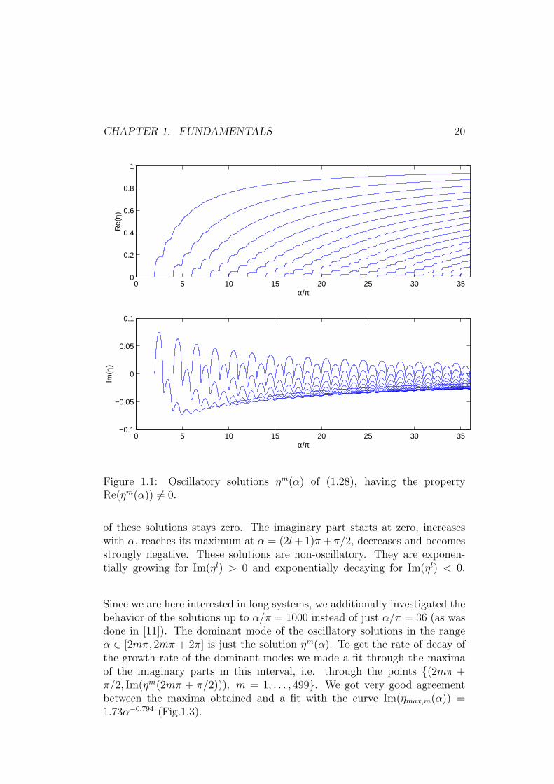
The solutions of this eigenfrequency equation depend on the normalizedlength α. In principle the method of choice is to find all analytic solutionsη(α) and to then perform the limit α → ∞. However, this is not feasible ana-lytically because the eigenfrequency equation is a sum of an exponential termand a polynomial in α. Hence we have solved (1.28) numerically using valuesfrom the numerical solutions given in [11] as starting values. The results of[11] were confirmed (Figs. 1.1 and 1.2). One can identify two different setsof solutions. The first set ηm(α) is characterized by the property that thestarting point of the curve is at 2mπ, m ∈ N (Fig.1.1). The real part of thesesolutions starts at zero, increases with α and tends to 1 for α → ∞. Theimaginary part also starts at zero, increases with α, reaches its maximum atα = 2mπ +π/2, decreases and gets negative. These solutions are oscillatory;they are unstable (exponentially) for Im(ηm) > 0 and stable (exponentiallydecaying) for Im(ηm) < 0.

The second set of solutions ηl(α) is characterized by the property that thestarting point of the curve is at (2l + 1)π, l ∈ N0 (Fig.1.1). The real part


0 5 10 15 20 25 30 350

0.2

0.4

0.6

0.8

1

α/π

Re(

η)

0 5 10 15 20 25 30 35−0.1

−0.05

0

0.05

0.1

α/π

Im(η

)

Figure 1.1: Oscillatory solutions ηm(α) of (1.28), having the propertyRe(ηm(α)) 6= 0.

of these solutions stays zero. The imaginary part starts at zero, increaseswith α, reaches its maximum at α = (2l + 1)π + π/2, decreases and becomesstrongly negative. These solutions are non-oscillatory. They are exponen-tially growing for Im(ηl) > 0 and exponentially decaying for Im(ηl) < 0.

Since we are here interested in long systems, we additionally investigated thebehavior of the solutions up to α/π = 1000 instead of just α/π = 36 (as wasdone in [11]). The dominant mode of the oscillatory solutions in the rangeα ∈ [2mπ, 2mπ + 2π] is just the solution ηm(α). To get the rate of decay ofthe growth rate of the dominant modes we made a fit through the maximaof the imaginary parts in this interval, i.e. through the points {(2mπ +π/2, Im(ηm(2mπ + π/2))), m = 1, . . . , 499}. We got very good agreementbetween the maxima obtained and a fit with the curve Im(ηmax,m(α)) =1.73α−0.794 (Fig.1.3).


0 5 10 15 20 25 30 350

0.02

0.04

0.06

0.08

0.1

0.12

0.14

0.16

0.18

α/π

Im(η

)

Figure 1.2: Purely growing solutions ηl(α) of (1.28), having the propertyRe(ηl(α)) = 0.

The analogous procedure for the curves ηl(α), i.e., for the non-oscillatorymodes with α = (2l + 1)π + π/2 also leads to excellent agreement with thecurve Im(ηmax,l(α)) = 1.15α−0.827 (Fig.1.4).

One can estimate the rate of decay of the growth rates using the dispersionrelation (1.28). We will show this estimation for the set of non-oscillatorysolutions ηl(α), the set of oscillatory solutions ηm(α) can be treated analo-gously. Inserting η = iηi and α = (2l+1)π+π/2 in (1.28) and approximating1 + η2

i by 1 (we consider growth rates much smaller than 1) leads to

− exp(−αηi) + αη2i + 2ηi = 0.

Inserting the ansatz ηi(α) = cα−d leads to

− exp(−cα1−d) + cα1−2d + 2cα−d = 0. (1.29)

We restrict our analysis to the case c > 0 and consider the limit α → ∞. Ford > 1 the first term becomes constant and the last two terms go to zero, so


0 100 200 300 400 500 600 700 800 900 100010

−3

10−2

10−1

100

α/π

Loca

l max

ima

of Im

(η)

Numerical solutionFitted asymptotic behaviour

Figure 1.3: Fit through the local maxima of the imaginary part of the set ofcurves ηm(α), i.e., for the oscillary modes.

equation (1.29) can not be fulfilled. For d < 1/2 the first term goes to zeroand the second term goes to infinity, so equation (1.29) can not be fulfilled.Thus we have restricted the coefficient d to the range

d ∈ [1/2 , 1] .

A comparison with the coefficients of the fits given above (d = 0.827 for theoscillatory solution and d = 0.794 for the non-oscillatory solution) shows,that indeed d is in the required range.

Summarizing this section we can say that the eigenfrequency equation of thePierce diode has unstable solutions for each α. However, if we increase thelength of the system the growth rates of the most unstable solutions decay tozero. So at least for the special case of the Pierce Diode we showed that forbig enough systems the influence of the boundary on the stability propertiesof the plasma can be neglected. This is an argument for using the dispersionrelation of the unbounded plasma in section 2.


0 100 200 300 400 500 600 700 800 900 100010

−3

10−2

10−1

100

α/π

Loca

l max

ima

of Im

(η)

Numerical solutionFitted asymptotic behaviour

Figure 1.4: Fit through the local maxima of the set of curves ηl(α).

1.1.5 Instability of a Low-Density Beam passing throughthe plasma

In this section we look at instabilities of a cold, uniform, collisionless, infiniteplasma [8]. We neglect any boundary conditions because we assume that thesystem is long enough (Sec.1.1.4). We ignore not only the thermal particlemotion but also plasma nonuniformity, collisions between particles and anymagnetic field. We start with the more general situation where the plasma isassumed to consist of several directed monoenergetic particle beams movingrelative to each other so that the electron (or ion) distribution has the form

f(x, v) =∑

α

nαδ(v − uα),

where α designates the beam and nα and uα are the density and velocity ofthe particles of beam α, respectively. We restrict ourselves to electrostatic


perturbations and get (with E = −∇φ) the following set of basic equations

∂nα

∂t+ ∇ · (nαuα) = 0

∂uα

∂t+ (uα · ∇)uα =

e

mα

E

∂2

∂x2φ =

e

ǫ0

∑

α

nα.

In this case the dispersion relation can be written ([8]) as

1 +∑

α

ǫα0 = 0, with ǫα

0 = −(ωα

p )2

(ω − kuα0 )2

. (1.30)

It is obtained assuming small perturbations of the form

Xα = Xα0 + X

′α(k, ω) exp(i(kx − ωt))

which leads to the linearized basic equations (omitting for convenience thesuperscript α)

−iωn′ + ∇ · (n′u0 + n0u′) = 0

−iωu′ + (u0 · ∇)u′ + (u′ · ∇)u0 =e

mE ′

Using the continuity and momentum equation and also the uniformity as-sumptions

∇n0 = 0 and ∇u0 = 0

we obtain the perturbation of the density n′ as a function of the potential.Substituting this function in Poisson’s equation

k2φ =e

ǫ0

∑

α

nα

and assuming quasineutrality∑

α

enα0 = 0

we obtain the dispersion relation (1.30).

Now we consider a plasma consisting of electrons and ions at rest and addi-tionally one low-density electron beam. We assume that the density of theelectron beam ne,beam is low compared with the density n of the primaryelectrons , i.e., the electrons at rest

ne,beam ≪ n.


We shall show that a system of this kind is unstable. Regarding the ions asa neutralizing background (thus the ion term is neglected) and omitting thesubscript in quantities X0 from now on) dispersion relation (1.30) becomes([8])

1 −ω2

p

ω2−

αω2p

(ω − k‖u)2= 0. (1.31)

Here we have α := ne,beam/n ≪ 1 and u is the velocity of the low densityelectron beam.

Note that this situation is a good approximation for the dispersion relationfor a low-density beam of secondary electrons in the presheath. Now wederive solutions with real part k‖u and group velocity ugr = u, where u isthe velocity of the secondary electrons. We will also provide growth rates ofthese solutions.

First we consider the dispersion relation (1.31) for the case α = 0,

(ω2 − ω2p)(ω − k‖u)2 − αω2

pω2 = 0. (1.32)

from which we readily obtain the four solutions

ω = ±k‖u and ω = ±ωp.

Hence, also for small α we expect two roots near ±k‖u which we will considerin the following part. For these two roots we assume |ω − ωp| ≫ |ω − k‖u|,approximate ω2 − ω2

p by (k‖u)2 − ω2p and obtain

((k‖u)2 − ω2p)(ω − k‖u)2 − αω2

pω2 = 0.

So instead of a polynomial equation of fourth order for ω we get a polynomialequation of second order which can be solved. The solution is

ω =k‖u

(

(k‖u)2 − ω2p

)

±√

αω2p(k‖u)2

(

(k‖u)2 − ω2p

)

(k‖u)2 − ω2p − αωp

.

Now due to the smallness of α we can use the following approximation forthe denominator

(k‖u)2 − ω2p − αωp ≈ (k‖u)2 − ω2

p,

then we cancel down and get

ω = k‖u ±√

αωp

√

1 −(

ωp/k‖u)2

.


If |k‖u| < ωp the term within the square root becomes negative and thesecond term of the derived expression for ω becomes complex. Choosing thepositive root we find the growth rate

γ = Im(ω) =√

αωp

√

(

ωp/k‖u)2 − 1

.

The group velocity is then

ugr =∂Re(ω)

∂k‖

=∂(k‖u)

∂k‖

= u.

Summary (instability of a low-density beam):Consider the dispersion relation (1.31) of a low-density beam (α := n1/n0 ≪1). Then for ω ≈ k‖u 6= ωp two of the four roots of (1.31) are equal to

ω = k‖u ±√

αωp

√

1 −(

ωp/k‖u)2

. (1.33)

If k‖u < ωp one of these roots is complex, corresponding to an instability withgrowth rate

γ = Im(ω) =√

αωp

√

(

ωp/k‖u)2 − 1

(1.34)

and group velocity u.

1.2 PIC Algorithms

1.2.1 Introduction to PIC Algorithms

The model underlying a PIC algorithm consists of charged particles movingunder the influence of forces due of their own and applied fields. The fieldsare calculated from Maxwell’s equations by knowing the positions and veloc-ities of all particles; the forces on the particles are found using the ensuingelectric and magnetic fields in the Newton-Lorentz equation of motion. Onecalculates the fields from the instantaneous macroscopic charge and currentdensities, then moves the particles (small time steps and distances) and re-calculates the macroscopic densities and fields due to the particles at theirnew positions and velocities; this procedure is repeated for many time steps.One can also extend the algorithm to allow for collisions between particles,a quite general scheme of a PIC algorithm is given in Fig.1.5


The fields are calculated on a spatial grid, which must be chosen fine enoughto resolve a Debye length. The grid provides a smoothing effect by notresolving spatial fluctuations that are smaller than the grid size. The use oftemporal and spatial grids, which are mathematical and not physical, causesconcern about accuracy and may create “unphysical effects”.

Figure 1.5: Scheme of a PIC-algorithm.

Let us now look at the algorithm in more detail. For simplicity we omitthe collision and the diagnostic blocks and focus on the calculation of theelectrostatic field and the particle mover. We also restrict ourselves to havinga constant external magnetic field present. The resulting scheme is shown inFig.1.6.

Since PIC algorithms are very time consuming, the spatial variable is mostoften 1-dimensional. By contrast, the velocity variable is most often 3-dimensional. An algorithm like this is said to have dimensionality (1d,3v)and is called a (1d, 3v) PIC algorithm.


Figure 1.6: Scheme of the simplified PIC-algorithm.

1.2.2 Particle and Force Weighting

A single particle is labeled by an index i, so that its velocity and positionis given by vi and xi. The field quantities will be obtained only on thespatial grid, consisting of discrete points in space labeled with index j itsvalue there being Ej. The ties from the particle positions and velocitiesto the field quantities are made by first calculating the charge and currentdensities on the grid, which requires stating how to produce the grid densitiesfrom the particle velocities and positions. This process of charge and currentassignment implies some weighting to the grid points that is dependent onthe particle position. With the fields known on the grid but the particlesscattered around in the grid, we then interpolate the fields from the grid tothe particles in order to apply the force at the particle by again performing aweighting. In principle the two weighting methods can be different, however


we use the same weighting in both density and force calculations in orderto avoid a self-force which would imply that a particle accelerates itself. Wenow describe the simplest weighting schemes.

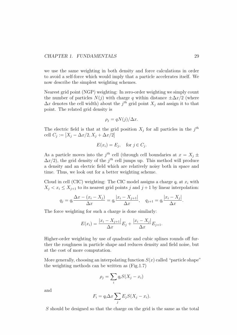
Nearest grid point (NGP) weighting: In zero-order weighting we simply countthe number of particles N(j) with charge q within distance ±∆x/2 (where∆x denotes the cell width) about the jth grid point Xj and assign it to thatpoint. The related grid density is

ρj = qN(j)/∆x.

The electric field is that at the grid position Xj for all particles in the jth

cell Cj := [Xj − ∆x/2, Xj + ∆x/2]

E(xi) = Ej, for j ∈ Cj.

As a particle moves into the jth cell (through cell boundaries at x = Xj ±∆x/2), the grid density of the jth cell jumps up. This method will producea density and an electric field which are relatively noisy both in space andtime. Thus, we look out for a better weighting scheme.

Cloud in cell (CIC) weighting: The CIC model assigns a charge qi at xi withXj < xi ≤ Xj+1 to its nearest grid points j and j +1 by linear interpolation:

qj = qi∆x − (xi − Xj)

∆x= qi

|xi − Xj+1|∆x

, qj+1 = qi|xi − Xj|

∆x.

The force weighting for such a charge is done similarly:

E(xi) =|xi − Xj+1|

∆xEj +

|xi − Xj|∆x

Ej+1.

Higher-order weighting by use of quadratic and cubic splines rounds off fur-ther the roughness in particle shape and reduces density and field noise, butat the cost of more computation.

More generally, choosing an interpolating function S(x) called “particle shape”the weighting methods can be written as (Fig.1.7)

ρj =∑

i

qiS(Xj − xi)

andFi = qi∆x

∑

j

EjS(Xj − xi).

S should be designed so that the charge on the grid is the same as the total


∆xS(x)

x∆x/2−∆x/2

NGP

∆xS(x)

x∆x−∆x

CIC

Figure 1.7: Interpolating functions for charge and force: NGP and CIC.

particle charge:

g∆x∑

j

ρj =∑

i

qi.

For a particle at position x it follows that

∆x∑

j

S(Xj − x) = 1.

The statement, in CIC and higher order interpolation,

∆x∑

j

XjS(Xj − x) = x

says that the charge at x makes the same, and correct contribution to dipolemoments independent of the particle location (∆x

∑

j ρjXj =∑

i qixi).

Additionally the algorithm should conserve the total momentum P . Thechange of the total momentum of the overall system dP/dt can be shown tobe

dP

dt=∑

i

Fi = ∆x∑

j

ρjEj.


In an infinite or periodic system, if the algorithm treats all grid points in thesame way and has left-right symmetry (reflection invariance), then

∆x∑

j

ρjEj = 0

and system momentum is conserved. In the presence of boundaries ∆x∑

j ρjEj 6=0 and total momentum is not conserved.

1.2.3 Particle Mover

In this section we describe how to update the positions and velocities ofthe charged particles using the Newton-Lorentz equation of motion. Onecommonly used method is called “leap-frog” method. The two first-orderdifferential equations to be integrated separately for each particle are

mdv

dt= F

dx

dt= v,

where F is the force. These equations are replaced with the finite-differenceequations

mvnew − vold

∆t= Fold

xnew − xold

dt= vnew.

Note that we are using a staggered time grid. This means that x and v arenot taken at the same time, but are shifted with respect to each other by∆t/2 (see also [10]). This shift is physically reasonable because we use v forthe transition between two positions. However, care must be taken in theinitialization step to take this time shift into account. Consider

F = qE + qv × B

with a uniform static magnetic field B = B0ez along z (the qv × B forcecorresponds just to a rotation of v) and E = Ex(t)ex is the electric fieldalong x (which alters the magnitude of vx). Set

ωc =qB

m


A physically reasonable (1d,2v) scheme (with t′ and t′′ as dummy variablest − ∆t/2 < t′ < t′′ < t + ∆t/2) which is centered with respect to time is asfollows:

Update of particle velocity

Half acceleration

(

vx(t′)

vy(t′)

)

=

(

vx(t − ∆t2

) + qm

Ex(t)∆t2

vy(t − ∆t2

)

)

Rotation(

vx(t′′)

vy(t′′)

)

=

(

cos(ωc∆t) sin(ωc∆t)−sin(ωc∆t) cos(ωc∆t)

)(

vx(t′)

vy(t′)

)

Half acceleration

(

vx(t + ∆t2

)vy(t + ∆t

2)

)

=

(

vx(t′′) + q

mEx(t)

∆t2

vy(t′′)

)

Update of particle position

x(t + ∆t) =

(

x(t) + v(t +∆t

2)∆t

)

.

1.2.4 Calculation of the electric field

Starting from the charge and current densities as assigned to the grid points,we now obtain the electric and magnetic fields, in general, from Maxwell’sequations, using ρ and j as sources. Here we take this step for an electrostaticproblem in one dimension x.

The differential equations to be solved are

E = −∂φ

∂x∂E

∂x=

ρ

ǫ0

,

which are combined to obtain Poisson’s equation

∂2φ

∂x2= − ρ

ǫ0

.


One approach ([22], also used in BIT1) is to solve the finite difference equa-tions as

Ej = −φj+1 − φj−1

2∆xφj+1 − 2φj + φj−1

(∆x)2= −ρj

ǫ0

The main computational burden lies in solving the resulting big system oflinear equations

Aφ = −(∆x)2

ǫ0

ρ,

where A is a large tridiagonal matrix.

1.2.5 The PIC Code BIT1

The (1d,3v) code BIT1 ([19]) was developed in Innsbruck on the basis of theXPDP1 code from the University of California at Berkeley. BIT1 has someimportant features: as the code from Berkeley it includes an external cir-cuit. It has a variety of built-in collisions and includes emission of secondaryelectrons from the wall.

1.2.5.1 Collisions

BIT1 contains the following types of collisions:

• Coulomb collisions [16]• Electron-neutral collisions [21]

- Elastic scattering- Excitation- Ionization

• Ion-neutral collisions [21]- Elastic scattering- Charge exchange

In a BIT1 simulation, neutrals are not implemented as particles, but as auniform background with density specified in the input file. The collisioncross-sections can be specified in three ways: first they can be put constant,second they can have a simple shape. The third and most sophisticated op-tion for charged-neutral collisions uses functions approximating experimentalresults for Hydrogen, Deuterium and Tritium [20], see Fig.1.8.


100

101

102

103

104

10−22

10−21

10−20

10−19

10−18

10−17

Energy [eV]

σ(E

) [m

2 ]

e−H: Elastic scatteringe−H: Excitatione−H: IonizationH−H: Elastic scatteringH−H: Charge exchange

Figure 1.8: Cross sections of e-H-collisions and H-H-collisions used for BIT1.

1.2.5.2 Secondary-Electron Emission

When particles hit the wall they can induce emission of secondary electrons(SEs). BIT1 offers three different ways of including secondary electrons. Thesimplest method is to use a constant secondary-electron emission coefficientγ, where γ is the proportion of secondary electrons coming from the wallrelative to the incoming particles.

The second method is based on experimental results for electron impactinduced secondary-electron emission [17], using the formula

γ = γ0δ(α)Ep

E0

exp[2+2√

Ep/E0)] for δ(α) =

{

1/ cos α if 1/ cos α ≤ 2

2 if 1/ cos α > 2.

Here, Ep is the primary-particle energy, α is the angle of the particle incidenceon the wall, and E0 and γ0 are constants which have to be specified in theinput file.


The third method is based on experimental results for ion impact inducedsecondary-electron emission [12], using the formula

γ = γ0δ(α)(vp − v0) for δ(α) =

{

1/ cos α if 1/ cos α ≤ 2

2 if 1/ cos α > 2.

Here, vp is the primary-particle velocity and v0 and γ0 are constants whichhave to be specified in the input file.

1.2.6 Practial Considerations

Running a good simulation is not trivial; a simulation program is not ablack box which works fine with standard parameters. Physical knowledgeis needed to correctly set parameters and to avoid unphysical effects. Forexample, choosing the time step ∆t too big can lead to wrong frequencies ofplasma oscillations (Fig.1.9). Poor simulations can even result in numericalinstabilities: e.g., the so-called leapfrog algorithm for the model of a simpleharmonic oscillator can lead to a nonphysical instability (Fig.1.10) if thetime step ∆t is chosen too large (∆t > 2/ω0, where ω0 is the frequency ofthe harmonic oscillator).

1.2.6.1 Basic simulation conditions

To ensure that the PIC algorithm works properly, some basic conditions mustbe fulfilled. To achieve Debye shielding, one must have enough computerparticles Nc within a Debye length λD, which must also be resolved by thespatial grid step. However the grid step must not be so small that a particlecan pass a whole grid cell during one time step ∆t. The time step mustbe small enough to resolve the fastest occurring oscillations ωmax (whichis the maximum of the plasma oscillation frequency ωp and the cyclotronfrequency ωc) [1]. Summarizing we get the following basic conditions for aproper simulation:

Nc

λD

≥ 50

∆x ≤ λD

∆x ≥ vmax∆t (1.35)

∆t ≤ 0.2

ωmax

Often vmax is chosen as 3vth or - if the heat flux has to be resolved accurately- as 5vth. Moreover one usually sets ∆x = λD/2 and Nc = 200 and chooses


0 0.2 0.4 0.6 0.8 1 1.2 1.4 1.6 1.8 20.9

1

1.1

1.2

1.3

1.4

1.5

1.6

∆t⋅ωp

ω/ω

p

Analytic result (Birdsall)From simulations with ES1

Figure 1.9: Effect of the finite time step on the frequency of plasma oscilla-tions: ω denotes the frequency of the simulation.

∆t small enough to satisfy the last two inequalities. The larger the systemthe more particles are needed, which has a big influence on the simulationtime. Simulations involving about 106 particles are feasible (depending onthe machine). Note that for the calculation of λD and vth one has to knowin advance the resulting density n and electron temperature Te.If one only wants to simulate the sheath, the conditions (1.35) are suffi-cient because one only has to simulate a region consisting of about 10 Debyelengths, so that Nc does notget too large. If, however, the simulation regionalso includes the presheath, collisions have to be accounted for and anothercondition has to be fulfilled. This is because in a BIT1 simulation neutralsform an artificial background. When a neutral is ionized, a new ion is createdbut the neutral background does not change. This can lead to the situationthat in the system more ions are produced than are lost to the wall. The


0 0.5 1 1.5 2 2.5 3 3.5 4−0.2

0

0.2

0.4

0.6

0.8

1

1.2

1.4

1.6

1.8

ω0∆t

ω⋅∆

t

Re(ω)Im(ω)

Figure 1.10: Effect of the finite time step for the leapfrog algorithm on thestability of the motion of a simple harmonic oscillator: ω and ω0 denote thefrequency of the simulation and of the harmonic oscillator, respectively ([1]).

particle balance (gain ≤ loss)

neνionV = ninnσionvthLA ≈ ni(SE)

λmfp

√

kBTe

me

LA =≤ nicSA ≈ ni

√

kBTe

mi

A,

leads to

L ≤√

me

mi

λmfp (1.36)

Here we took for simplicity ni = ni(SE), often ni(SE) = 0.5ni.For B 6= 0 additionally

∆t ≤ 0.35

ωp

must hold.


1.2.6.2 Particle Sources

BIT1 offers essentially two different kinds of particle sources: the sourcesmay be located in the middle of the system and/or at one or both of theboundaries. The ion and electron particle fluxes in the source have to beprescribed accurately according to physical considerations to avoid artificialresults.

Consider the case of the source being the right-hand boundary of the sim-ulation region which is also assumed to be at the sheath edge. First of allat the sheath edge we have quasineutrality ni = ne = n. At the right-handboundary we can only inject particles going to the left. So the incomingelectrons are assumed to have a half Maxwellian electron distribution withformal temperature Te, whose flux Γe is

Γe =nvth√

2π, with vth =

√

kBTe/me

The Bohm criterion requires that the average ion velocity at the sheathedge is the ion sound velocity. Therefore we assume the ion distributionat the right-hand boundary to be a shifted Maxwellian distribution withshift velocity vshift and a cut at v ≈ 0: The shift velocity has to be chosen sothat the mean ion velocity is just −cS. This leads to

vshift = −cS +

√

2

πvthe

−v2

shift/2v2

th

(

1 +1

erf(|vshift|/√

2vth)

)

With collisions the ion velocity distribution is not Maxwellian any more(Fig.1.11), so that setting up the flux is more complicated. One usually fixesthe ion flux at the value nvshift, where n is the density at the sheath edge(which is about half the density of the bulk plasma) and changes the inputflux of the electrons to avoid unphysical properties at the source. Essentiallyone ensures quasineutrality, which can be diagnosed with the density profile,but even better with the profile of the electric field. The problem is thatone really has to wait for steady state to judge the quality of the simulation.In order to save time the first trials can be made with a smaller number ofcomputer particles.


−16 −14 −12 −10 −8 −6 −4 −2 0 2 4

x 104

0

500

1000

1500

2000

2500

3000

3500

vx

f(v x)

Figure 1.11: Velocity distribution of ions, when charged-neutral collisions areon.

Chapter 2

Theoretical calculation of theinfluence of secondary electronson the stability of the PWT

Secondary electrons (SEs) are emitted from the wall due to the impact ofprimary particles (electrons or ions, but we will only consider electrons) onthe wall. Then they get accelerated in the sheath and enter the presheathas a distinct beam with a narrow velocity distribution function. If the cor-responding electron-beam instability is stronger than the damping processesin the presheath, the presheath becomes unstable. In this section we derivethe dispersion relation, the numerical solution of which shows that we canexpect an instability induced by the secondary electrons.

Figure 2.1: 1-D system considered for the calculation of a sufficient conditionfor presheath instability.

In this section we consider the 1-D system shown in Fig.2.1. The wall is at

40

CHAPTER 2. INFLUENCE OF SE ON PWT STABILITY 41

x = L, the sheath-presheath boundary at x = 0 and the presheath corre-sponds to negative values of x. The main calculation refers to the presheath.The sheath influences the presheath solution by imposing the appropriateboundary conditions at the sheath-presheath boundary. The boundary ofthe plasma is not explicitly included because of the justification of section1.1.4 where we showed that at least for the special case of the Pierce Diodefor long enough systems the influence of the boundary on the stability prop-erties of the plasma can be neglected. In what follows γ is the secondaryelectron emission coefficient, n0 is the plasma density at the presheath en-trance (x = 0), j is the current density, and cS =

√

kB(Te + Ti)/mi is the ionsound velocity. Here, the difference of this value for cS to the more generalvalue (1.20) is very small (of the order of a few percent).

2.1 Sheath in the presence of secondary elec-

trons

First we look at the sheath to get the appropriate boundary conditions forthe calculation of the presheath instability.

The Bohm criterion is the starting point for this calculation since it providesa value for the ion particle flux density from a plasma to the surface. A briefinvestigation showed that it also holds for simulations including secondaryelectrons. However, a more detailed investigation will be done in the nextfuture. Due to its small width we assume the sheath to be collisionless.Therefore the ion current entering the sheath (at x = 0) is the same as theion current reaching the surface (at x = L),

|ji(0)| = |ji(L)| = en0cS.

We are now in a position to derive an expression for secondary electron emis-sion from the surface, arising from electron impact, since this is significanteven at rather modest energies, Te ≥ 30eV . Note that here and in whatfollows primary electrons will have the index e and secondary electrons willhave the index se. By contrast, ion-induced secondary electron emission isusually only important for ion impact energies of ≥ 1keV . By definition ofthe secondary electron coefficient γ the secondary electron current density isthe fraction γ of the current density jpe of the incoming primary electrons

|jse(L)| = γ|je(L)|,So the secondary electrons decrease the net electron current

|je,tot(L)| = |je(L)| − |jse(L)| = (1 − γ)|je(L)|,


For je(L) we take the flux of a Maxwellian distribution flowing to a wall([14, 15])

|je(0)| = |je(L)| =1

4en0

√

8

πvth exp

(

e∆φ

kBTe

)

, vth =

√

kBTe

me

,

where ∆φ < 0 is the potential drop from the sheath edge to the wall. Thetotal current at the sheath edge is given by

j(0) = j(L) =: j = |ji(0)| − |je,tot(0)|,

which directly leads to

e∆φ

kBTe

= ln

(√2π(cS − j/en0)

(1 − γ)vth

)

. (2.1)

The secondary electrons are accelerated by the sheath potential from the wallto the sheath edge and reach the velocity

|use(0)| =

√

−2e∆φ

me

=√

2vth

√

−e∆φ

kBTe

.

Using equation (2.1) this leads to

|use(x = 0)| = η0vth, η0 =

√

2 ln

(

(1 − γ)vth√2π(cS − j/en0)

)

% 1. (2.2)

2.2 Presheath Model

The calculations below are based on the model given in [18]. We considera plasma presheath with one ion species. As boundary condition at thesheath entrance (x = 0) we assume that the secondary electrons enter thepresheath with a velocity use equal to or higher than the plasma electronthermal velocity (2.2). We additionally have as boundary conditions φ(x =0) = 0, quasineutrality (ni = ne = n0) and the Bohm criterion ui = cS.

For the primary electron temperature Te we assume the typical range 10eV ≤Te ≤ 100eV . We assume that secondary electrons have zero velocity directlyafter their creation at the wall, so their energy spread is very small comparedto the energy spread of the primary electrons. This condition allows us to usea cold-beam approximation for the secondary electrons. The computationalpart of this thesis suggests that a relaxation of this condition may be desir-able, because the energy of the secondary electrons can spread due to the


induced instability. However this will be a future refinement of the theory.We also assume η0 to be of order unity.

From section 1.1.5 we expect an oscillation frequency ω ≈ kuse % kvth. Theplasma electrons must be described with a kinetic model, whereas the ionsand secondary electrons will be treated hydrodynamically.

Assuming isothermal ions and plasma electrons and neglecting terms of theorder me/mi, nse/ne and ue/vth, we write the following system of equationsdescribing the plasma presheath. The system consists of the continuity andmomentum equations for ions and secondary electrons, the kinetic equationfor the plasma electrons and - since we only consider electrostatic waves -the Poisson equation.

∂

∂tni +

∂

∂xniui = neνion

∂

∂tnse +

∂

∂xnseuse = 0

∂

∂tui + ui

∂

∂xui +

e

mi

∂

∂xφ = − 1

mini

∂

∂xnikBTi − (νin + νion)ui − νie(ui − ue)

∂

∂tuse + use

∂

∂xuse −

e

me

∂

∂xφ = −νseuse (2.3)

∂

∂tfe(x, v) + v

∂

∂xfe(x, v) +

e

me

∂φ

∂x

∂

∂vfe(x, v) = −νe(fe − f0)

f0(x, v) =n0

e(x)√2πvth

exp(−v2/2v2th)

∂2

∂x2φ =

e

ǫ0

(ne + nse − ni)

Here ne =∫

fedv, ue = n−1e

∫

vfedv and the ν’s are the characteristic fre-quencies for different collisions (see [18] and Table 2.1). Λ is the Coulomb-logarithm: 10 ≤ Λ ≤ 18. In the table, the temperature and density are givenin eV and m−3, respectively.

The right-hand side of the momentum equation for the secondary electrons isνseuse and does not contain the difference between use and ui or ue, becauseuse is much bigger than ui and ue, so ui and ue are neglected.

In order to use the cold-beam approximation for the secondary electrons weassume the friction to be sufficiently small:

∂

∂xuse ∼

use

δx∼ vth

δx≫ νse, (2.4)

where δx is the scale length of the presheath inhomogeneity.


ν Collision accounts for Formula Valueνion electron impact ionization σion(Te, ne)vthnn 6 · 104

νin ion-neutral elastic and charge exchange σivthnn 105

νie ion-electron collision momentum transfer 1.48 · 10−12Λnme/miT3/2e 50

νcse SE with ions and primary electrons 2.41 · 106Λn/|use|3 2 · 106

νnse SE with neutrals (elastic+excitation) 〈σel+exv〉nn 6 · 105

νse SE with ions, primary electrons, neutrals νcse + νn

se 3 · 106

νe elastic collisions of plasma electrons 5 · 10−12ΛnT3/2e 3 · 105

Table 2.1: Formulas and typical values for collision frequencies for n =1018m−3, nn = 1019m−3, Te = 30eV, Ti = 15eV, Λ = 10 and Hydrogenions.

2.3 Zeroth order solution

Now we make an ansatz

Θ(x, t) = Θ0(x) + Θ1(x)ei(ωt−kx), Θ0 ≫ Θ1, k ≫ ∂

∂xln Θ0,1, (2.5)

where Θ denotes the physical quantities ne,i,se, ue,i,se, fe entering the basicequations. Now we will insert the ansatz (2.5) into the model, retain zero-order terms and obtain the system describing the presheath in the time-independent state. First we define

M := u0i /cS, νsum := νion + νin, and a :=

√

νion + νin

νion

.

(i) Densities: We start with the 0th order equation for the primary electrons,

∂

∂tf 0

e + v∂

∂xf 0

e +e

me

∂φ0

∂x

∂

∂vf 0

e = −νe(f0e − f0)

Substituting f 0e = f0 in this equation leads to

∂n0e(x)

∂x=

e

me

∂φ0

∂xne(x)/v2

th.

Dividing by n0e(x), integrating over x and taking the exponential of the result

we obtain

n0e(x) = n0 exp

(

eΦ

kBTe

)

. (2.6)


Assuming approximate quasineutrality in 0th order means that n0i (x) =

n0e(x) =: n0(x). The total current to the wall, which is the same as the

current at the sheath edge, consists of the ion and the electron part

j = n0i u

0i − je(wall) = n0cS − (1 − γ)je,wall = n0cS − 1 − γ

γjse.

Thus, using jse = −en0sev

0se = en0

seη0vth,

n0se =

1 − γ

γ

n0cS − j

η0vth

.

(ii) Ion velocity: Starting with the 0th-order ion momentum equation

u0i

∂u0i

∂x+

e

mi

∂φ0

∂x= − Ti

min

∂n0

∂x− νsumu0

i ,

we substitute ∂φ0/∂x by n using the Boltzmann relation (2.6), to obtain

u0i

∂u0i

∂x+

c2S

n0

∂n0

∂x= −νsumu0

i . (2.7)

We can express ∂n0/∂x by terms including u0i using the continuity equation,

yielding

(u0i −

c2S

u0i

)∂u0

i

∂x+

c2Sνion

u0i

= −νsumu0i .

This is a differential equation with separated variables. Thus we multiply byu0

i , put the terms with u0i on the left side and the rest on the right side, and

integrate:

u0i∫

u0i,0

u2 − c2S

c2Sνion + νsumu2

du =cS

νion

M∫

1

M2 − 1

1 + M2νsum/νion

dM = −x∫

0

dx = −x

(2.8)To evaluate the integral on the left-hand side we first make the substitutionz = M

√

νsum/νion =: aM and rewrite it in the form

cS

νion

1

a2

aM∫

a

z2 − a2

1 + z2

dz

a=

cS

νion

1

a3

aM∫

a

(1 + z2) − (1 + a2)

1 + z2dz

Evaluating this and combining it with the right-hand side of (2.8) leads to

M − 1 −(

1

a+ a

)

(arctan ((aM) − arctan(a)) = −a2νion

cS

x = −νsum

cS

x.


(iii) Potential: We start with equation (2.7) in the form

u0i

∂u0i

∂x+ c2

S

∂

∂xln(n0) = −νsumu0

i

and the continuity equation

0 =1

n0

∂

∂x(n0u0

i ) − νion = u0i

∂

∂xln(n0) +

∂u0i

∂x− νion.

In order to remove the term −νsumu0i , we multiply the former equation by ν

and the latter equation by νsumui, and add both equations to obtain

(c2Sνion + νsumu2

i )∂

∂xln(n0) = −(νion + νsum)u0

i

∂u0i

∂x= −1

2(νion + νsum)

∂(u0i )

2

∂x.

So∂

∂xln(n0) = −1

2(νion + νsum)

∂M2/∂x

νion + νsumM2.

Now we get φ using the Boltzmann equation

φ =kBTe

eln(n0) =

kBTe

e

x∫

x0

∂

∂xln(n0)dx =

kBTe

e

νion + νin/2

νsum

ln

(

νion + νsumM0

νion + νsumM2

)

.

Note, that the boundary condition φ0(x = 0) = 0 is fulfilled forM0 = M(x = 0) = 1.

Summary: (time-independent state)The 0th-order solution of the model (2.3) with the boundary conditions

φ0(x = 0) = 0, M(x = 0) = 1, u0se(x = 0) = −η0vth

has the following form:

f 0e (x, v) = f0(x, v)

n0i = n0

e =: n = n0 exp

(

eφ0

kBTe

)

1 − νsum

cS

x = M −(

a +1

a

)

(arctan(aM) − arctan(a))

φ0 =kBTe

e

νion + νin/2

νsum

ln

(

2νion + νin

M2νsum + νion

)

(2.9)

n0se =

γ

1 − γ

n0cS − j/e

η0vth

u0se

∂

∂xu0

se = − e

me

∂

∂xφ0 − νseu

0se


for

f0(x, v) =n0

e(x)√2πvth

exp(−v2/2v2th), νsum = νion + νin

and

a =

√

νion + νin

νion

, M = u0i /cS, cS =

√

kBTe

mi

.

The 0th-order solution (2.9) has the following structure. The electron and iondensity, n0

e(x) and n0i (x), are both given by the Boltzmann term exp(eφ/kBTe)

(thus we have quasineutrality in the presheath), the electrons being Maxwellian.The ion velocity u0

i (x) is given by an implicit equation. The potential φ0 isalso space-dependent (φ0 = φ0(M(x))).

The velocity of the secondary electrons is still given by the differential equa-tion

u0se

∂

∂xu0

se = − e

me

∂

∂xφ − νseu

0se (2.10)

which, however, can be solved numerically because φ0 is now known. Fig.2.2shows the numerical solution of the differential equation for use for varioussecondary-electron emission coefficients γ. We obtained the solution usingthe simple explicit Adams method [9]). In each step of the Adams methodin order to evaluate φ0(x) we have to obtain M(x) from the equation

1 − νsum

cS

x = M −(

a +1

a

)

(arctan(aM) − arctan(a)) (2.11)

and insert this into (2.9), so that we obtain φ0(x) = φ0(M(x)). In our simu-lations the wall is at the left side. For easier comparisons with simulations inFig.2.2 the presheath is in the positive halfspace and the presheath entranceis at x = 0.

We see that |u0se| increases monotonically from the sheath-presheath bound-

ary (x=0). For increasing γ the value of |u0se| decreases and reaches the

minimal value for γc = 0.81. The value γc is the critical value (for a hy-drogen plasma), for which in the sheath no monotonic solution for φ exists([5]).

A good approximation for the maximum value at the end of the presheath is

|u0se|max/vth ≈

√

η20 +

2νion + νin

νion + νin

ln(2 + νin/νion). (2.12)

To obtain this result we make the following approximation in the differentialequation for u0

se (2.10), which can be made because of the weak friction


0 0.005 0.01 0.015 0.02 0.025 0.03 0.035 0.04

1.4

1.6

1.8

2

2.2

2.4

2.6

x

u se0/v

th,e

γ = 0.1γ = 0.3γ = 0.7γ = 0.83Approximation

Figure 2.2: Numerical solution for the secondary-electron velocity for varioussecondary electron emission coefficients γ.

condition (2.4),

u0se

∂

∂xu0

se =1

2

∂

∂x(u0

se)2 = −νseu

0se +

e

me

∂

∂xφ0 ≈ e

me

∂

∂xφ0,

from which we obtain

(u0se)

2max = u0

se(−L)2 ≈ u0se(0)2 +

−L∫

0

2e

me

∂φ0

∂xdx ≈ η2

0v2th +

2eφ0(−L)

me

, (2.13)

where we already used φ0(x = 0) = 0. From equation (2.9) we find φ0(x =−L) = φ0(M = 0)

φ0(x = −L) =kBTe

e

νion + νin/2

νsum

ln

(

2νion + νin

νion

)

.

Substitution of φ0(−L) in (2.13) leads to (2.12). Formula (2.12) holds verywell (Fig.2.2). For later use we note that η ≥ 1.3 holds everywhere in oursystem.


2.4 First-order solution

The next step consists in solving the time-independent first-order equations.We first derive the dispersion relation which we then approximately solve forthe region near the end of the presheath, to obtain a sufficient condition forthe presheath instability.

(i) We start out with the first-order Poisson equation,

∂2

∂x2φ1ei(ωt−kx) = −k2φ1 =

e

ǫ0

(n1e + n1

se) (2.14)

Note that in deriving this equation we have neglected certain terms in accor-dance with the assumption k ≫ ∂

∂xΘ0,1.

(ii) Now we insert the appropriate expressions for the densities into the Pois-son equation (2.14). The secondary-electron density n1

se is found from thefirst-order continuity and momentum equations for the secondary electrons.The former equation has the form

∂

∂tn1

seei(ωt−kx) +

∂

∂x

(

n0seu

1see

i(ωt−kx) + n1see

i(ωt−kx)u0se

)

= 0

which leads to

n1se =

kn0seu

1se

ω − ku0se

. (2.15)

As before we have neglected some terms involving ∂Θ0,1/∂x. Before insert-ing this term into Poissons equation we calculate u1

se from the first-ordermomentum equation

−νseu1see

i(ωt−kx) =∂

∂tu1

seei(ωt−kx) + u0

se

∂

∂xu1

seei(ωt−kx)

+u1see

i(ωt−kx) ∂

∂xu0

se +e

me

∂

∂xφ1ei(ωt−kx).

Neglecting terms proportional to ∂Θ0,1/∂x as before and performing thederivatives we find

u1se = − ke

me

φ1/(ω − ku0se − iνse).

Substituting u1se in equation (2.15) we obtain the desired equation for n1

se

(note that u0se < 0, so we can write |u0

se| instead of −u0se)

n1se = −k2φ1 en0

se/me

(ω + k|u0se|)(ω + k|u0

se| − iνse).


Now we substitute the expression found for the first-order secondary-electrondensity and the first-order primary-electron density

n1e =

∫

dvf 1e

in Poisson’s equation (2.14) to obtain

−k2φ1 =e

ǫ0

(∫

dvf 1e − k2φ1 en0

se/me

(ω + k|u0se|)(ω + k|u0

se| − iνse)

)

Using the definition of the plasma frequency ωp and defining

α :=n0

se

n0

we can rewrite this as

φ1 = φ1αω2

p

(ω + k|u0se|)(ω + k|u0

se| − iνse)− e

ǫ0k2

∫

dvf 1e (2.16)

(iii) In the last step we have to treat the primary electron term using thefirst-order kinetic equation for the electrons

−νef1e ei(ωt−kx) =

∂

∂tf 1

e ei(ωt−kx) + v∂

∂xf 1

e ei(ωt−kx)

+e

me

∂f 0e

∂v

∂

∂xφ1ei(ωt−kx) +

e

me

∂φ0

∂x

∂

∂vf 1

e ei(ωt−kx)

Neglecting terms with ∂Θ0,1/∂x and taking the derivatives we find

(ω − kv − iνe)f1e =

ek

me

∂f 0e

∂vφ1

Now we can solve this equation for f 1e and substitute the latter in equation

(2.16),

1 =αω2

p

(ω + k|u0se|)(ω + k|u0

se| − iνse)− e2

ǫ0kme

∫

dv∂f 0

e /∂v

ω − kv − iνe

(2.17)

(iv) Now we focus on the term with the integral. Substituting f 0e and differ-

entiating with respect to v, yields

e2

ǫ0kme

ne(x)√2πvthv2

th

∫

dvv exp(−v2/2v2

th)

ω − kv − iνe

.


On simplifying the constants in front of the integral and multiplying thenominator and denominator by −k we find

− 1

k2λ2D

1√2πvth

∫

dv[(ω − kv − iνe) + (−ω + iνe)] exp(−v2/2v2

th)

ω − kv − iνe

.

In the second term we make the substitution t = v/√

2vth, which leads to

− 1

k2λ2D

1√2πvth

(√2vth

∫

dte−t2 +ω − iνe√

2kvth

√2vth

∫

dtexp(−t2)

t − (ω − iνe)/√

2kvth

)

.

The first integral is well known to be√

π, the second is equal to√

πZ((ω −iνe)/

√2kvth), so we can write it as

− 1

k2λ2D

(

1 +y√2Z

(

y√2

))

with

y :=ω − iνe

kvth

.

Summary (dispersion relation):Collecting terms of first order in the system (2.3) one obtains the dispersionrelation

1 =αω2

p

(ω + k|u0se|)(ω + k|u0

se|) − iνse

− 1

k2λ2D

(

1 − J+

(

ω − iνe

kvth

))

(2.18)

with

α := n0se/n, J+(y) = − y√

2Z

(

y√2

)

, Z(y) =1√π

∞∫

−∞

1

t − ye−t2dt.

A purely numerical treatment of the dispersion relation using the “pseudoarclength”continuation method ([4]) shows the following unstable solution branch (Fig.2.3).

Equation (2.18) can be considered as a dispersion relation only if the homoge-neous plasma approximation is valid, i.e., the characteristic time of instabilitygrowth 1/|Im(ω)| is much smaller than the time the wave packet needs to“feel” the plasma inhomogeneity (δx/ugr):

|Imω| ≫ 1

δx

∂ω

∂k∼ νin + νion

cS

|u0se| ∼ (νin + νion)η

√

mi

2me

(2.19)


0 1 2 3 4 5 6 70

0.005

0.01

0.015

0.02

0.025

0.03

0.035

0.04

kλD

|Im(ω

)|/ω

p

γ = 0.3γ = 0.7

Figure 2.3: Numerical solution for the growing branch of the dispersion re-lation (2.18) for various values of γ.

Let us now take a closer look at the dispersion relation. Using the weak-friction (2.4) and the homogeneity condition (2.19) we will obtain a sufficientcondition for the presheath instability.

We first want to find an expression for the imaginary part of the growing solu-tion of (2.18). Multiplying the dispersion relation (2.18) by the denominatorleads to

[(ω + k|u0se|)2 − iνse(ω + k|u0

se|)][1 + (1 − J+(y))/k2λ2D] = αω2

p

Solving this quadratic equation for ω + k|u0se| we obtain

ω ≈ ku0se + i

νse

2±√

αω2p

1 + (1 − J+(y))/k2λ2D

− ν2se

4. (2.20)

Next we derive an expression for the imaginary part of the growing solution


of (2.20)

Im(ω) =νse

2± Im

(

√

αω2p

1 + (1 − J+(y))/k2λ2D

− ν2se

4

)

. (2.21)

To do this we must to find an expression for a term having the form Im(√

c + ib).On one hand √

c + ib2

= c + ib,

on the other hand√

c + ib2

= (Re(√

c + ib) + Im(√

c + ib))2 = Re2 − Im2 + 2iReIm.

Comparing the imaginary parts we obtain Re = b/2Im. Substituting Re inthe equation resulting from the comparison of the real parts we find

(

Im2)2

+ cIm2 − b2/4 = 0.

Solving this quadratic equation for Im2 and taking the square root we obtain

Im = ± 1√2

√

−c ±√

c2 + b2.

If c > 0 (we will show later that c > 0 holds) we must take the plus sign infront of the second root to get a real number because

√c2 + b2 > |c|. This

yields

Im = ± 1√2

√

−c +√

c2 + b2. (2.22)

Multiplying the denominator of the fraction term of the root of (2.21) with itsconjugate complex we can identify c with −ν2

se/4−αω2pA and b with −αω2

pBfor

A :=k2λ2

D(ReJ+(y) − 1 − k2λ2D)

(ReJ+(y) − 1 − k2λ2D)2 + (ImJ+(y))2

and

B :=k2λ2

DImJ+(y)

(ReJ+(y) − 1 − k2λ2D)2 + (ImJ+(y))2

.

Using equation (2.22) with c and b above equation (2.21) results in

Im(ω) =νse

2± 1√

2

√

√

√

√

ν2se

4+ αω2

p

(

A

√

(

ν2se

4αω2p

+ A

)2

+ B2

)

Due to the inhomogeneity and weak friction assumptions we can neglect νse

because

Im(ω) ≫ 1

∂x

∂ω

∂k∼ |u0

se|(νin + νion)

cS

∼ ηmi

me

(νin + νion) ∼ νse.


Since we are searching for instabilities with Im(ω) < 0 we must take theminus sign in front of the root. Therefore we obtain

Im(ω) ≈ −√

αωp√2

√

A +√

A2 + B2. (2.23)

For typical values (such as kλD = 0.65 (Fig.2.3) and Re(y) ≈ 1.3 (Fig.2.2)and small Im(y)) A is negative which means that c > 0. Using (2.23) thehomogeneity condition (2.19) can be written as

CI :=

√αωp

√

A +√

A2 + B2

η√

mi/me(νin + νion)≫ 1. (2.24)

To find out if we can expect an instability we can numerically solve thedispersion relation (now with νse neglected) in order to obtain ω(kλD). Thenwe calculate A(y(ω(kλD))) and B(y(ω(kλD))) as functions of kλD and insertit in (2.24) (Fig.2.4). Figure 2.4 shows that we can expect an instabilityinduced by the secondary electrons for kλD slightly less than 1.


0 0.2 0.4 0.6 0.8 1 1.2 1.4 1.6 1.8 20

2

4

6

8

10

12

14

16

kλD

CI

γ = 0.7

Figure 2.4: Instability criterion: for CI ≫ 1 we expect instability.

Chapter 3

Simulations

In this section we compare the results of the theory with results from sim-ulations performed with BIT1. We will demonstrate in the simulation theinstability which is induced by the secondary electrons. Based on the simu-lation results we additionally propose a mechanism which limits the growthof the instability.

3.1 Simulation Setup

The simulations were all done with the same version of the BIT1 code. Theparameters are chosen so as to satisfy the conditions of section 1.2.6.1. Asource on the right-hand boundary injects the particles (Fig.3.1). Note thatin the simulation the wall is not at the left-hand side (as in the model) butat the right-hand side because more diagnostics are available at the left wall.

For the ion and electron particle fluxes entering at the right-hand boundarywe first calculated

ΓR,i =nvth,i√

2πand ΓR,e =

nvth,e√2π

and then adjusted the electron particle flux to ensure quasineutrality at theright-hand side. Every output is averaged over 4096 time steps correspondingto about 115 plasma oscillations νp = ωp/2π. In the input-file of the code theparticle species used in the simulation are defined by their masses, charges,input conditions et cetera. The simulations treat the secondary electrons inthe same way as the primary electrons. For the purpose of obtaining all the

56

CHAPTER 3. SIMULATIONS 57

Figure 3.1: Simulation region.

diagnostics for the secondary electrons (especially their mean velocity andtheir velocity distribution) we additionally had to perform simulations wherethey were treated as a separate species.

The most important parameters of the simulation are given in table 3.1.

variable description valuenc number of cells 400

nc2p number of real particles per computer particle 8 · 106

dt time step 3.5 · 10−12

L length of the system 0.02 marea area of the system 10−4 mnfft number of time steps for the FFT 4096nn neutral density 4 · 1019 m−3

Tn temperature of neutrals 0.001 eVΓR,e Electron injection flux at the right wall 7.7 · 1023

TR,e temperature of injected electrons 30 eVΓR,i Ion injection flux at the right wall 2.14 · 1022

TR,i temperature of injected ions 30 eV

Table 3.1: Description of the most important input parameters

The final simulations included about 200000 electrons and 200000 ions. Withγ = 0.7, about 6800 secondary electrons were in the simulation, which means17 secondary electrons per cell.


3.2 Basic Plasma Parameters

In this section we look at the influence of the secondary electrons on thebasic plasma parameters such as density, potential, electric field, temperatureand mean velocities. Figures 3.2 and 3.3 show that, in accordance withthe theoretical results, in the presheath the basic plasma parameters do notchange with changing secondary-electron emission coefficient γ. This doesnot hold for the sheath (Fig.3.4), where the potential drop is observed todepend on γ. Comparing in table 3.2 the value for the potential drop obtainedfrom the simulation (the sheath edge was taken as the position where theplasma gets quasineutral) with the theoretical values [5] given in equation(3.1), we find good agreement between theory and simulation

− e∆Φ

kBTe

= ln

(

1 − γ√

2πm/M

)

. (3.1)

γ e∆Φ/kBTe from (3.1) e∆Φ/kBTe from simulation0 2.84 2.87

0.3 2.48 2.520.7 1.64 1.64

Table 3.2: Potential drop in the presheath from theory and from simulation


0 0.002 0.004 0.006 0.008 0.01 0.012 0.014 0.016 0.018 0.020

2

4

6

8

10x 10

17

x [m]

Ele

ctro

n de

nsity

[m−

3 ] γ = 0γ = 0.3γ = 0.7

0 0.002 0.004 0.006 0.008 0.01 0.012 0.014 0.016 0.018 0.02−100

−50

0

50

x [m]

Pot

entia

l [eV

]

γ = 0γ = 0.3γ = 0.7

0 0.002 0.004 0.006 0.008 0.01 0.012 0.014 0.016 0.018 0.02−6

−4

−2

0

2x 10

5

x [m]

Ele

ctric

fiel

d [e

V/m

] γ = 0γ = 0.3γ = 0.7

0 0.002 0.004 0.006 0.008 0.01 0.012 0.014 0.016 0.018 0.02−2.5

−2

−1.5

−1

−0.5

0

x [m]

Ion

velo

city

M =

ui/c

S γ = 0γ = 0.3γ = 0.7

Figure 3.2: Density, potential, electric-field and ion-velocity profiles for thewhole simulation region.


0 0.002 0.004 0.006 0.008 0.01 0.012 0.014 0.016 0.018 0.02−6

−5

−4

−3

−2

−1

0x 10

5

x [m]

Ele

ctro

n ve

loci

ty u

e [m/s

]

γ = 0γ = 0.3γ = 0.7

0 0.002 0.004 0.006 0.008 0.01 0.012 0.014 0.016 0.018 0.026

8

10

12

14

16

18

20

x [m]

Ion

tem

pera

ture

Ti [e

V]

γ = 0γ = 0.3γ = 0.7

0 0.002 0.004 0.006 0.008 0.01 0.012 0.014 0.016 0.018 0.0222

24

26

28

30

x [m]

Ele

ctro

n te

mpe

ratu

re T

e [eV

] γ = 0γ = 0.3γ = 0.7

Figure 3.3: Electron-velocity, electron-temperature and ion-temperature pro-files for the whole simulation region.


0 0.2 0.4 0.6 0.8 1

x 10−3

0

2

4

6x 10

17

x [m]

Den

sity

[m−

3 ]

ElectronsIons

0 0.2 0.4 0.6 0.8 1

x 10−3

−100

−80

−60

−40

−20

0

x [m]

Pot

entia

l [eV

]

γ = 0γ = 0.3γ = 0.7

0 0.2 0.4 0.6 0.8 1

x 10−3

−6

−4

−2

0x 10

5

x [m]

Ele

ctric

fiel

d [e

V/m

] γ = 0γ = 0.3γ = 0.7

0 0.2 0.4 0.6 0.8 1

x 10−3

−2.5

−2

−1.5

−1

−0.5

x [m]

Ion

velo

city

M =

ui/c

S γ = 0γ = 0.3γ = 0.7

Figure 3.4: Density, potential, electric-field and ion-velocity profiles in thesheath region.


3.3 Check of the zeroth order model

In this section we compare the simulation results with those of the zeroth-order model (2.9).

There clearly are some differences between theory and simulation. The firstdifference concerns the ion temperature. As specified in the input-file the ionsinjected at the right boundary are not cold (Fig.3.3), the ion-temperaturedepends on the position x. The electron and ion densities depend on theposition as well. Consequently the collision frequencies, which mostly dependon the temperature and/or the density become space-dependent, too. Evenif these collision frequencies were not dependent on x, it would still not bestraightforward to compare them with the collision frequencies of the modelbecause the collision frequencies of the model account for the momentumtransfer, whereas those of the code account for the number of collisions.

To compare model and simulation we take the collision frequencies of thesimulation as first guesses and then vary them slightly manually for thepurpose of fitting the mean ion-velocity profile (M(x)) using (2.11). Thenwe obtain the potential and density profile in a stepwise manner. Using(2.9) we find the potential profile φ0(x) = φ0(M(x)). Substituting φ0(x)in the Boltzmann relation (2.6) we then obtain the density profile n0(x) =n0(φ0(M(x))). To distinguish differences coming from the current step todifferences from all the previous steps we additionally make hybrid models.There we use the mean ion velocity of the simulation instead of the meanion velocity of the model and the potential of the simulation instead of thepotential of the model in step two and three, respectively.

For the mean ion velocity we get a rough fit (Fig.3.5, upper panel) whichis good at the sheath-side and gets worse in the direction of the right-handboundary. This is not surprising because the use of (2.11) ensures that themean ion velocity is equal to the sound velocity at the sheath edge. Surpris-ingly in the next step this rough fit for the mean ion velocity leads to verygood agreement with the potential obtained from the simulation (Fig.3.5,middle panel). The fit is even better than the fit where we used the meanion velocity obtained from the simulation. The potential of the simulationhas a slight decrease at the right wall which is more likely a source effect ofthe simulation. The lowest panel of Fig.3.5 shows that in the last step thedensity profile can be excellently predicted by the Boltzmann relation us-ing the potential profile obtained from the simulation. Also the pure modelworks quite well. At the right wall again the source effect can be identified.


0 0.002 0.004 0.006 0.008 0.01 0.012 0.014 0.016 0.018 0.020.2

0.4

0.6

0.8

1

1.2

x [m]

M =

v/c

S

ModelSimulation

0 0.002 0.004 0.006 0.008 0.01 0.012 0.014 0.016 0.018 0.02−10

0

10

20

30

x [m]

Pot

entia

l [eV

]

ModelHybrid modelSimulation

0 0.002 0.004 0.006 0.008 0.01 0.012 0.014 0.016 0.018 0.024

6

8

10

12x 10

17

x [m]

Den

sity

[m−

3 ]

ModelHybrid modelSimulation

Figure 3.5: Comparison of theory with simulations. Density, potential, ion-velocity and secondary-electron-velocity profiles. The hybrid model for thepotential uses the ion velocity from the simulation in equation (2.9), thehybrid model for the density uses the potential obtained from the simulationin Boltzmann’s relation (2.6).


Figure 3.6 shows a comparison of the mean velocity of the secondary electronsobtained from the simulation with the velocity obtained from the numericalsolution of the differential equation (2.10). The mean secondary electronvelocity for both simulation and numerical solution increases entering thepresheath at the sheath edge. However, while the numerical solution contin-ues to increase, u0

se taken from the simulation decreases. We account this lackof fit to the instability which is induced by the secondary electron beam. Wewill see later (Fig.3.13) that also the temperature of the secondary electronsincreases during the penetration of the presheath. This happens approxi-mately at the same position where the numerical solution and the simulationbegin to show different behaviours regarding u0

se.

0 0.002 0.004 0.006 0.008 0.01 0.012 0.014 0.016 0.018 0.021.4

1.5

1.6

1.7

1.8

1.9

2

2.1

2.2

x [m]

u se0/v

th,e

Numerical solutionSimulation

Figure 3.6: Mean velocity of secondary electrons u0se obtained from the sim-

ulation and from the numerical solution of differential equation (2.10) (bothfor γ = 0.7).

Figure 3.7 shows that the electrons are approximately Maxwellian distributed.

In contrast to the electrons the ion-velocity distribution is clearly not Maxwellian(Fig.3.8) due to collisions (especially due to charge exchange collisions withthe cold neutral background). At the position x = 0.0018 which is still insidethe presheath the ions are already clearly accelerated by the potential of thepresheath.

In Fig.3.9 we check the density of the secondary electrons (2.9) which shouldonly depend on γ (not on x). We plot α := n0

se/n0 dependent on γ and


−1 −0.8 −0.6 −0.4 −0.2 0 0.2 0.4 0.6 0.8 1

x 107

0

50

100

150

200

250

vx

f(v x)

SimulationFitted Maxwellian

Figure 3.7: Electron-velocity distribution.

compare the result with the simulations performed with γ = 0.3 and γ = 0.7.In the simulation the secondary electron density is not constant but slightlydepends on x. Therefore we plot a bar from the minimum to the maximumvalue of the secondary electron density and obtain good agreement with (2.9).


−4 −3 −2 −1 0 1 2 3 4

x 104

0

50

100

150

200

250

vx

f(v x)

Ions at x=0.01Ions at x=0.001825

Figure 3.8: Ion-velocity distribution at two different positions in thepresheath.

0 0.1 0.2 0.3 0.4 0.5 0.6 0.7 0.80

0.01

0.02

0.03

0.04

0.05

0.06

0.07

0.08

γ

α =

nse

/n0

ModelSimulation

Figure 3.9: Comparison of theory with simulations. Density of the secondaryelectrons dependent on the secondary electron emission coefficient γ.


3.4 Instability

3.4.1 Detection of the Instability

In this section we demonstrate the instability in the simulation. For thispurpose we look at the frequency spectrum of the potential at two differentpositions (Fig.3.10). We clearly see that the peak which is near the plasmafrequency is increasing with increasing secondary electron emission coefficientγ.

6 6.5 7 7.5 8 8.5 9 9.5 10

x 109

0

10

20

30

40

V(f

) at

x=

0.01

γ = 0γ = 0.3γ = 0.7

6 6.5 7 7.5 8 8.5 9 9.5 10

x 109

0

10

20

30

40

V(f

) at

x=

0.00

1

γ = 0γ = 0.3γ = 0.7

Figure 3.10: Instability induced by secondary electrons for two different val-ues of the secondary electron emission coefficient γ for two different positions.


To ensure that the instabilities shown in Fig.3.10 do not have numericalreasons we did the same simulations with four times more computer parti-cles (800000 per species). Also in these simulations the instability could bedemonstrated (Fig.3.11). The instability for γ = 0.3 can be identified evenbetter than in the simulation using fewer computer particles.

6 6.5 7 7.5 8 8.5 9 9.5 10

x 109

0

10

20

30

40

V(f

) at

x=

0.01

γ = 0γ = 0.3γ = 0.7

6 6.5 7 7.5 8 8.5 9 9.5 10

x 109

0

10

20

30

40

V(f

) at

x=

0.00

1

γ = 0γ = 0.3γ = 0.7

Figure 3.11: Instability induced by secondary electrons for two different val-ues of the secondary electron emission coefficient γ for two different positionsfor the simulation with four times more simulation particles.


3.4.2 Saturation of the Instability

3.4.2.1 The Penrose criterion

Let us look at the mechanism which we conjecture to be responsible for stop-ping the growth of the instability. As the starting point for the explanationwe state the Penrose criterion (Fig.3.12) [2].

vA

vB

v

f(v)

Figure 3.12: Penrose criterion: beam-plasma distribution function.

The Penrose criterion asserts that the condition

∞∫

−∞

f(v) − f(vA)

(v − vA)2dv > 0

is a necessary and sufficient criterion for instabilities. The existence of aminimum of the electron velocity distribution is not, of itself, a sufficient cri-terion for instability. In effect, the minimum must be deep enough. However,in our case it turned out that even a very shallow minimum is sufficient forthe development of an instability.

The Penrose criterion is not directly applicable to our system because it con-siders the collisionless case with ions treated as a homogeneous background.However, it can be viewed as an approximative instability-treatment. ThePenrose criterion will give us a hint how the growth of the instability isstopped.


3.4.2.2 The saturation mechanism

Examining the diagnostics of the runs with three species we observed thatthe temperature of the secondary electrons strongly depends on the positionx (Fig.3.13). We conjectured that the observed temperature rise could affectthe result of the application of the Penrose criterion.

0 0.005 0.01 0.015 0.020

0.5

1

1.5

2

2.5

x [m]

T [e

V]

Temperature of secondary electrons

γ = 0.3γ = 0.7

Figure 3.13: Secondary-electron-temperature profile for two different valuesof the secondary electron emission coefficient γ.

To apply the Penrose criterion we consider the total electron velocity dis-tribution consisting of the primary electron distribution and the secondaryelectron distribution. If the system contains enough cold and fast secondaryelectrons the total distribution should have a minimum. Penetrating thepresheath the secondary-electron-temperature rises and their velocity distri-bution flattens leading to a shallower minimum of the total-electron-velocitydistribution. When the minimum is shallow enough the Penrose criterion isnot fulfilled any more and the instability saturates. To examine this behaviorin the simulations we compared the total electron distribution for several po-sitions and observed the expected behavior of the total electron distribution(Fig.3.14).

Note again that the Penrose criterion is not directly applicable to our system.


−1 −0.5 0 0.5 1

x 107

0

0.005

0.01

0.015

0.02

0.025

vx [m/s]

f(v x)

at x=0.001at x=0.003at x=0.015

Figure 3.14: The consequence of the flattening of the secondary-electron-velocity distribution for the total-electron-velocity distribution for γ = 0.7.

Therefore in the near future we plan to revise the model of chapter 2 wherethe secondary-electrons are not considered to be cold any more.

Chapter 4

Conclusion and future work

In this thesis the influence of secondary-electrons on the stability of thepresheath was investigated using both theory (section 2) and particle sim-ulations (section 3). Secondary-electrons are emitted from the wall due tothe impact of primary particles. They get accelerated by the sheath po-tential and enter the presheath as a fast beam where they may induce thecorresponding electron-beam instability.

The calculation of the theoretical part refers to the collisional presheath. Thesheath influences the presheath solution by imposing the appropriate bound-ary conditions at the sheath-presheath boundary. Three particle species areconsidered: ions, primary electrons and cold secondary-electrons. Secondary-electrons enter the presheath with a velocity equal or higher than the plasmaelectron thermal velocity. At the sheath-presheath boundary also quasineu-trality and the Bohm criterion are prescribed. First the stationary statesolution is found (section 2.3). The following main calculation includes thederivation of the dispersion relation (section 2.4). The numerical solution ofthe dispersion relation shows that an instability induced by the secondaryelectrons can be expected.

Particle-in-cell (PIC) simulations showed (in accordance with theory) nochange of the basic plasma parameters with changing secondary electronemission coefficient in the presheath . In the sheath we observed a dependenceof the potential drop on the secondary electron emission coefficient which isin very good agreement with theoretical results [5]. Only with respect to thesecondary-electron-velocity theory and simulation show qualitative disagree-ment which we account to the instability induced by the secondary-electrons.The instability induced by the secondary electrons could be clearly demon-strated in the frequency spectrum of the potential. Identical simulations

72

CHAPTER 4. CONCLUSION AND FUTURE WORK 73

performed with four times more particles confirmed that the observed insta-bility does not have numerical reasons.

In addition to these already known [18] results we propose a mechanism re-sponsible for the saturation of the instability. Examining the simulations weobserved that the temperature of the initially cold secondary-electrons in-creases in the direction away from the wall. As a consequence the secondary-electron-velocity distribution flattens leading to a shallower minimum of thetotal-electron-velocity distribution. When the minimum is shallow enoughthe Penrose criterion is not fulfilled any more and the instability saturates.

To confirm the proposed saturation mechanism future investigations will in-clude an appropriate theory treating the secondary-electrons not any moreas cold. Additional simulations will be performed with secondary-electronshaving a finite temperature directly after their generation at the wall.

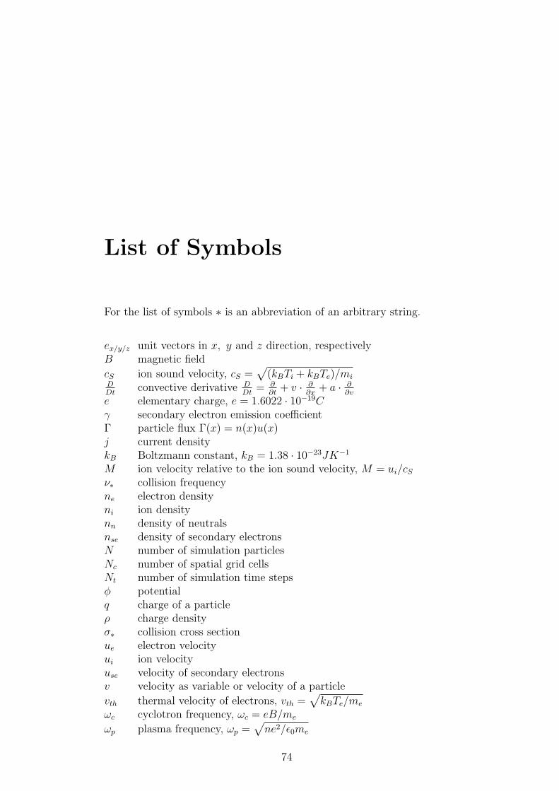
List of Symbols

For the list of symbols ∗ is an abbreviation of an arbitrary string.

ex/y/z unit vectors in x, y and z direction, respectivelyB magnetic field

cS ion sound velocity, cS =√

(kBTi + kBTe)/miDDt

convective derivative DDt

= ∂∂t

+ v · ∂∂x

+ a · ∂∂v

e elementary charge, e = 1.6022 · 10−19Cγ secondary electron emission coefficientΓ particle flux Γ(x) = n(x)u(x)j current densitykB Boltzmann constant, kB = 1.38 · 10−23JK−1

M ion velocity relative to the ion sound velocity, M = ui/cS

ν∗ collision frequencyne electron densityni ion densitynn density of neutralsnse density of secondary electronsN number of simulation particlesNc number of spatial grid cellsNt number of simulation time stepsφ potentialq charge of a particleρ charge densityσ∗ collision cross sectionue electron velocityui ion velocityuse velocity of secondary electronsv velocity as variable or velocity of a particle

vth thermal velocity of electrons, vth =√

kBTe/me

ωc cyclotron frequency, ωc = eB/me

ωp plasma frequency, ωp =√

ne2/ǫ0me

74

List of Figures

1 General structure of the PWT region without magnetic field. . 7

1.1 Oscillatory solutions ηm(α) of (1.28), having the property Re(ηm(α)) 6= 0. 20

1.2 Purely growing solutions ηl(α) of (1.28), having the property Re(ηl(α)) = 0. 21

1.3 Fit through the local maxima of the imaginary part of the set of curves ηm(α), i.e., for

1.4 Fit through the local maxima of the set of curves ηl(α). . . . . 23

1.5 Scheme of a PIC-algorithm. . . . . . . . . . . . . . . . . . . . 27

1.6 Scheme of the simplified PIC-algorithm. . . . . . . . . . . . . 28

1.7 Interpolating functions for charge and force: NGP and CIC. . 30

1.8 Cross sections of e-H-collisions and H-H-collisions used for BIT1. 34

1.9 Effect of the finite time step on the frequency of plasma oscillations: ω denotes the frequency

1.10 Effect of the finite time step for the leapfrog algorithm on the stability of the motion of

1.11 Velocity distribution of ions, when charged-neutral collisions are on. 39

2.1 1-D system considered for the calculation of a sufficient condition for presheath instabilit

2.2 Numerical solution for the secondary-electron velocity for various secondary electron emission

2.3 Numerical solution for the growing branch of the dispersion relation (2.18) for various

2.4 Instability criterion: for CI ≫ 1 we expect instability. . . . . . 55

3.1 Simulation region. . . . . . . . . . . . . . . . . . . . . . . . . . 57

75

LIST OF FIGURES 76

3.2 Density, potential, electric-field and ion-velocity profiles for the whole simulation region.

3.3 Electron-velocity, electron-temperature and ion-temperature profiles for the whole sim

3.4 Density, potential, electric-field and ion-velocity profiles in the sheath region. 61

3.5 Comparison of theory with simulations. Density, potential, ion-velocity and secondary-electron-v

3.6 Mean velocity of secondary electrons u0se obtained from the simulation and from the n

3.7 Electron-velocity distribution. . . . . . . . . . . . . . . . . . . 65

3.8 Ion-velocity distribution at two different positions in the presheath. 66

3.9 Comparison of theory with simulations. Density of the secondary electrons dependent

3.10 Instability induced by secondary electrons for two different values of the secondary electron

3.11 Instability induced by secondary electrons for two different values of the secondary electron

3.12 Penrose criterion: beam-plasma distribution function. . . . . . 69

3.13 Secondary-electron-temperature profile for two different values of the secondary electron

3.14 The consequence of the flattening of the secondary-electron-velocity distribution for the

List of Tables

2.1 Formulas and typical values for collision frequencies for n = 1018m−3, nn = 1019m−3, T

3.1 Description of the most important input parameters . . . . . . 57

3.2 Potential drop in the presheath from theory and from simulation 58

77

Bibliography

[1] C.K. Birdsall and A.B. Langdon 1985. Plasma physics via computersimulation. McGraw-Hill Book Company.

[2] T.J.M. Boyd and J.J. Sanderson 2002. The Physics of Plasmas. Cam-bridge University Press.

[3] F.F. Chen 1984. Plasma physics and controlled fusion. Vol1: plasmaphysics. Plenum Press, New York.

[4] G. Eibl 1997. Diploma thesis: Numerische Verfahren zur Berechnungvon Losungszweigen nichtlinearer Gleichungssysteme.

[5] G.D. Hobbs and J.A. Wesson 1967. Heat flow through a Langmuir sheathin the presence of electron emission. Plasma Physics, 9, 85-87.

[6] S. Kuhn and M. Horhager 1986. External-circuit effects on Pierce-diodestability behavior. J. Appl. Phys., 60, 1952-59.

[7] S. Kuhn 1994. The physics of bounded plasma systems (BPS’s): Simu-lation and interpretation. Contrib. Plasma Phys., 34 (4), 495-538.

[8] A.B. Mikhailovskii 1974. Theory of plasma instabilities, Vol.1: Instabili-ties of a homogeneous plasma. Consultants Bureau, New York, London.

[9] A. Ostermann. Lecture “Numerische Losung gewohnlicher Differential-gleichungen”

[10] S.V. Patankar 1980. Numerical heat transfer and fluid flow.

[11] W. Pfendt 1991. Diploma thesis “Zur analytischen Beschreibung desschwach nichtlinearen Verhaltens der Pierce-Diode”. Institute of Theo-retical Physics, University Innsbruck.

[12] A. Quayyum et al. 2003. Electron emission and molecular fragmentationduring hydrogen and deuterium ion impact on carbon surfaces. J. Nucl.Mat. 313-316.

78

BIBLIOGRAPHY 79

[13] K.-U. Riemann 2000. Theory of the plasma-sheath transition. J. Tech.Phys., 41 (1), Special Issue, 89-121.

[14] R. Schrittwieser winter semester 2002/2003 Lecture about plasma diag-nostics

[15] P.C. Stangeby 2000. The plasma boundary of magnetic fusion devicesInstitute of Physics Publishing, Bristol and Philadelphia

[16] T. Takizuka and H. Abe 1977. A binary collision model for plasma sim-ulation with a particle code J. Comput. Phys., 25, 205-219.

[17] E.W. Thomas 1984. Secondary electron emission. Nucl. Fusion, DataCompendium for Plasma-Surface Interactions, Special Issue

[18] D. Tskhakaya and S. Kuhn 2000. Influence of secondary electrons onthe stability of the plasma-wall transition, 2000 International Congresson Plasma Physics (ICPP) combined with the 42nd APS-DPP-Meeting,Quebec City, Canada, 23-27 Oct 2000, Vol.1, 89-92. Bull.APS 45 (7),334, Abstr. VP1 27.

[19] D. Tskhakaya and S. Kuhn, 2002. Effect of E×B Drift on the PlasmaFlow at the Magnetic Presheath Entrance. Contrib. Plasma Phys., 42(2-4), 302-308.

[20] D. Tskhakaya and S. Kuhn 2002. Particle simulations of the magnetizedhydrogen plasma-wall transition taking into account collisions with hy-drogen. 29th Conference on Plasma Phys. and Contr. Fusion Montreux,17-21 June 2002 ECA Vol.26B, P-2.094.

[21] V. Vahedi and M. Surendra 1995. A Monte Carlo collision model for theparticle-in-cell method: applications to argon and oxygen dischargesComp. Phys. Com., 87, 179-198.

[22] J.P. Verboncoeur, M.V. Alves, V. Vahedi and C.K. Birdsall 1993. Simul-taneous potential and circuit solution for 1D bounded plasma particlesimulation codes Journal of computational physics, 104, 321-328.

particle-in-cell (pic) simulation of the plasma sheath and

Documents