partially linear models - preterhuman.netcdn.preterhuman.net/texts/math/partially linear...
TRANSCRIPT

PARTIALLY LINEAR MODELS
Wolfgang Hardle
Institut fur Statistik und OkonometrieHumboldt-Universitat zu Berlin
D-10178 Berlin, Germany
Hua LiangDepartment of StatisticsTexas A&M University
College StationTX 77843-3143, USA
and
Institut fur Statistik und OkonometrieHumboldt-Universitat zu Berlin
D-10178 Berlin, Germany
Jiti GaoSchool of Mathematical Sciences
Queensland University of TechnologyBrisbane QLD 4001, Australia
andDepartment of Mathematics and Statistics
The University of Western AustraliaPerth WA 6907, Australia

ii
In the last ten years, there has been increasing interest and activity in the
general area of partially linear regression smoothing in statistics. Many methods
and techniques have been proposed and studied. This monograph hopes to bring
an up-to-date presentation of the state of the art of partially linear regression
techniques. The emphasis of this monograph is on methodologies rather than on
the theory, with a particular focus on applications of partially linear regression
techniques to various statistical problems. These problems include least squares
regression, asymptotically efficient estimation, bootstrap resampling, censored
data analysis, linear measurement error models, nonlinear measurement models,
nonlinear and nonparametric time series models.
We hope that this monograph will serve as a useful reference for theoretical
and applied statisticians and to graduate students and others who are interested
in the area of partially linear regression. While advanced mathematical ideas
have been valuable in some of the theoretical development, the methodological
power of partially linear regression can be demonstrated and discussed without
advanced mathematics.
This monograph can be divided into three parts: part one–Chapter 1 through
Chapter 4; part two–Chapter 5; and part three–Chapter 6. In the first part, we
discuss various estimators for partially linear regression models, establish theo-
retical results for the estimators, propose estimation procedures, and implement
the proposed estimation procedures through real and simulated examples.
The second part is of more theoretical interest. In this part, we construct
several adaptive and efficient estimates for the parametric component. We show
that the LS estimator of the parametric component can be modified to have both
Bahadur asymptotic efficiency and second order asymptotic efficiency.
In the third part, we consider partially linear time series models. First, we
propose a test procedure to determine whether a partially linear model can be
used to fit a given set of data. Asymptotic test criteria and power investigations
are presented. Second, we propose a Cross-Validation (CV) based criterion to
select the optimum linear subset from a partially linear regression and estab-
lish a CV selection criterion for the bandwidth involved in the nonparametric
v

vi PREFACE
kernel estimation. The CV selection criterion can be applied to the case where
the observations fitted by the partially linear model (1.1.1) are independent and
identically distributed (i.i.d.). Due to this reason, we have not provided a sepa-
rate chapter to discuss the selection problem for the i.i.d. case. Third, we provide
recent developments in nonparametric and semiparametric time series regression.
This work of the authors was supported partially by the Sonderforschungs-
bereich 373 “Quantifikation und Simulation Okonomischer Prozesse”. The second
author was also supported by the National Natural Science Foundation of China
and an Alexander von Humboldt Fellowship at the Humboldt University, while the
third author was also supported by the Australian Research Council. The second
and third authors would like to thank their teachers: Professors Raymond Car-
roll, Guijing Chen, Xiru Chen, Ping Cheng and Lincheng Zhao for their valuable
inspiration on the two authors’ research efforts. We would like to express our sin-
cere thanks to our colleagues and collaborators for many helpful discussions and
stimulating collaborations, in particular, Vo Anh, Shengyan Hong, Enno Mam-
men, Howell Tong, Axel Werwatz and Rodney Wolff. For various ways in which
they helped us, we would like to thank Adrian Baddeley, Rong Chen, Anthony
Pettitt, Maxwell King, Michael Schimek, George Seber, Alastair Scott, Naisyin
Wang, Qiwei Yao, Lijian Yang and Lixing Zhu.
The authors are grateful to everyone who has encouraged and supported us
to finish this undertaking. Any remaining errors are ours.
Berlin, Germany Wolfgang Hardle
Texas, USA and Berlin, Germany Hua Liang
Perth and Brisbane, Australia Jiti Gao

CONTENTS
PREFACE . . . . . . . . . . . . . . . . . . . . . . . . . . . . . . . . . . . v
1 INTRODUCTION . . . . . . . . . . . . . . . . . . . . . . . . . . . . 1
1.1 Background, History and Practical Examples . . . . . . . . . . . . 1
1.2 The Least Squares Estimators . . . . . . . . . . . . . . . . . . . . 12
1.3 Assumptions and Remarks . . . . . . . . . . . . . . . . . . . . . . 14
1.4 The Scope of the Monograph . . . . . . . . . . . . . . . . . . . . . 16
1.5 The Structure of the Monograph . . . . . . . . . . . . . . . . . . . 17
2 ESTIMATION OF THE PARAMETRIC COMPONENT . . . 19
2.1 Estimation with Heteroscedastic Errors . . . . . . . . . . . . . . . 19
2.1.1 Introduction . . . . . . . . . . . . . . . . . . . . . . . . . . 19
2.1.2 Estimation of the Non-constant Variance Functions . . . . 22
2.1.3 Selection of Smoothing Parameters . . . . . . . . . . . . . 26
2.1.4 Simulation Comparisons . . . . . . . . . . . . . . . . . . . 27
2.1.5 Technical Details . . . . . . . . . . . . . . . . . . . . . . . 28
2.2 Estimation with Censored Data . . . . . . . . . . . . . . . . . . . 33
2.2.1 Introduction . . . . . . . . . . . . . . . . . . . . . . . . . . 33
2.2.2 Synthetic Data and Statement of the Main Results . . . . 33
2.2.3 Estimation of the Asymptotic Variance . . . . . . . . . . . 37
2.2.4 A Numerical Example . . . . . . . . . . . . . . . . . . . . 37
2.2.5 Technical Details . . . . . . . . . . . . . . . . . . . . . . . 38
2.3 Bootstrap Approximations . . . . . . . . . . . . . . . . . . . . . . 41
2.3.1 Introduction . . . . . . . . . . . . . . . . . . . . . . . . . . 41
2.3.2 Bootstrap Approximations . . . . . . . . . . . . . . . . . . 42
2.3.3 Numerical Results . . . . . . . . . . . . . . . . . . . . . . 43
3 ESTIMATION OF THE NONPARAMETRIC COMPONENT 45
3.1 Introduction . . . . . . . . . . . . . . . . . . . . . . . . . . . . . . 45

viii CONTENTS
3.2 Consistency Results . . . . . . . . . . . . . . . . . . . . . . . . . . 46
3.3 Asymptotic Normality . . . . . . . . . . . . . . . . . . . . . . . . 49
3.4 Simulated and Real Examples . . . . . . . . . . . . . . . . . . . . 50
3.5 Appendix . . . . . . . . . . . . . . . . . . . . . . . . . . . . . . . 53
4 ESTIMATION WITH MEASUREMENT ERRORS . . . . . . 55
4.1 Linear Variables with Measurement Errors . . . . . . . . . . . . . 55
4.1.1 Introduction and Motivation . . . . . . . . . . . . . . . . . 55
4.1.2 Asymptotic Normality for the Parameters . . . . . . . . . 56
4.1.3 Asymptotic Results for the Nonparametric Part . . . . . . 58
4.1.4 Estimation of Error Variance . . . . . . . . . . . . . . . . 58
4.1.5 Numerical Example . . . . . . . . . . . . . . . . . . . . . . 59
4.1.6 Discussions . . . . . . . . . . . . . . . . . . . . . . . . . . 61
4.1.7 Technical Details . . . . . . . . . . . . . . . . . . . . . . . 61
4.2 Nonlinear Variables with Measurement Errors . . . . . . . . . . . 65
4.2.1 Introduction . . . . . . . . . . . . . . . . . . . . . . . . . . 65
4.2.2 Construction of Estimators . . . . . . . . . . . . . . . . . . 66
4.2.3 Asymptotic Normality . . . . . . . . . . . . . . . . . . . . 67
4.2.4 Simulation Investigations . . . . . . . . . . . . . . . . . . . 68
4.2.5 Technical Details . . . . . . . . . . . . . . . . . . . . . . . 70
5 SOME RELATED THEORETIC TOPICS . . . . . . . . . . . . . 77
5.1 The Laws of the Iterated Logarithm . . . . . . . . . . . . . . . . . 77
5.1.1 Introduction . . . . . . . . . . . . . . . . . . . . . . . . . . 77
5.1.2 Preliminary Processes . . . . . . . . . . . . . . . . . . . . 78
5.1.3 Appendix . . . . . . . . . . . . . . . . . . . . . . . . . . . 79
5.2 The Berry-Esseen Bounds . . . . . . . . . . . . . . . . . . . . . . 82
5.2.1 Introduction and Results . . . . . . . . . . . . . . . . . . . 82
5.2.2 Basic Facts . . . . . . . . . . . . . . . . . . . . . . . . . . 83
5.2.3 Technical Details . . . . . . . . . . . . . . . . . . . . . . . 87
5.3 Asymptotically Efficient Estimation . . . . . . . . . . . . . . . . . 94
5.3.1 Motivation . . . . . . . . . . . . . . . . . . . . . . . . . . . 94
5.3.2 Construction of Asymptotically Efficient Estimators . . . . 94
5.3.3 Four Lemmas . . . . . . . . . . . . . . . . . . . . . . . . . 97

CONTENTS ix
5.3.4 Appendix . . . . . . . . . . . . . . . . . . . . . . . . . . . 99
5.4 Bahadur Asymptotic Efficiency . . . . . . . . . . . . . . . . . . . 104
5.4.1 Definition . . . . . . . . . . . . . . . . . . . . . . . . . . . 104
5.4.2 Tail Probability . . . . . . . . . . . . . . . . . . . . . . . . 105
5.4.3 Technical Details . . . . . . . . . . . . . . . . . . . . . . . 106
5.5 Second Order Asymptotic Efficiency . . . . . . . . . . . . . . . . . 111
5.5.1 Asymptotic Efficiency . . . . . . . . . . . . . . . . . . . . 111
5.5.2 Asymptotic Distribution Bounds . . . . . . . . . . . . . . 113
5.5.3 Construction of 2nd Order Asymptotic Efficient Estimator 117
5.6 Estimation of the Error Distribution . . . . . . . . . . . . . . . . 119
5.6.1 Introduction . . . . . . . . . . . . . . . . . . . . . . . . . . 119
5.6.2 Consistency Results . . . . . . . . . . . . . . . . . . . . . . 120
5.6.3 Convergence Rates . . . . . . . . . . . . . . . . . . . . . . 124
5.6.4 Asymptotic Normality and LIL . . . . . . . . . . . . . . . 125
6 PARTIALLY LINEAR TIME SERIES MODELS . . . . . . . . 127
6.1 Introduction . . . . . . . . . . . . . . . . . . . . . . . . . . . . . . 127
6.2 Adaptive Parametric and Nonparametric Tests . . . . . . . . . . . 127
6.2.1 Asymptotic Distributions of Test Statistics . . . . . . . . . 127
6.2.2 Power Investigations of the Test Statistics . . . . . . . . . 131
6.3 Optimum Linear Subset Selection . . . . . . . . . . . . . . . . . . 136
6.3.1 A Consistent CV Criterion . . . . . . . . . . . . . . . . . . 136
6.3.2 Simulated and Real Examples . . . . . . . . . . . . . . . . 139
6.4 Optimum Bandwidth Selection . . . . . . . . . . . . . . . . . . . 144
6.4.1 Asymptotic Theory . . . . . . . . . . . . . . . . . . . . . . 144
6.4.2 Computational Aspects . . . . . . . . . . . . . . . . . . . . 150
6.5 Other Related Developments . . . . . . . . . . . . . . . . . . . . . 156
6.6 The Assumptions and the Proofs of Theorems . . . . . . . . . . . 157
6.6.1 Mathematical Assumptions . . . . . . . . . . . . . . . . . 157
6.6.2 Technical Details . . . . . . . . . . . . . . . . . . . . . . . 160
APPENDIX: BASIC LEMMAS . . . . . . . . . . . . . . . . . . . . . 183
REFERENCES . . . . . . . . . . . . . . . . . . . . . . . . . . . . . . . . 187

x CONTENTS
AUTHOR INDEX . . . . . . . . . . . . . . . . . . . . . . . . . . . . . . 199
SUBJECT INDEX . . . . . . . . . . . . . . . . . . . . . . . . . . . . . 203
SYMBOLS AND NOTATION . . . . . . . . . . . . . . . . . . . . . . 205

1INTRODUCTION
1.1 Background, History and Practical Examples
A partially linear regression model of the form is defined by
Yi = XTi β + g(Ti) + εi, i = 1, . . . , n (1.1.1)
where Xi = (xi1, . . . , xip)T and Ti = (ti1, . . . , tid)
T are vectors of explanatory vari-
ables, (Xi, Ti) are either independent and identically distributed (i.i.d.) random
design points or fixed design points. β = (β1, . . . , βp)T is a vector of unknown pa-
rameters, g is an unknown function from IRd to IR1, and ε1, . . . , εn are independent
random errors with mean zero and finite variances σ2i = Eε2
i .
Partially linear models have many applications. Engle, Granger, Rice and
Weiss (1986) were among the first to consider the partially linear model
(1.1.1). They analyzed the relationship between temperature and electricity us-
age.
We first mention several examples from the existing literature. Most of the
examples are concerned with practical problems involving partially linear models.
Example 1.1.1 Engle, Granger, Rice and Weiss (1986) used data based on the
monthly electricity sales yi for four cities, the monthly price of electricity x1,
income x2, and average daily temperature t. They modeled the electricity demand
y as the sum of a smooth function g of monthly temperature t, and a linear
function of x1 and x2, as well as with 11 monthly dummy variables x3, . . . , x13.
That is, their model was
y =13∑j=1
βjxj + g(t)
= XTβ + g(t)
where g is a smooth function.
In Figure 1.1, the nonparametric estimates of the weather-sensitive load for
St. Louis is given by the solid curve and two sets of parametric estimates are
given by the dashed curves.

2 1. INTRODUCTION
FIGURE 1.1. Temperature response function for St. Louis. The nonparametric es-timate is given by the solid curve, and the parametric estimates by the dashedcurves. From Engle, Granger, Rice and Weiss (1986), with permission from theJournal of the American Statistical Association.
Example 1.1.2 Speckman (1988) gave an application of the partially linear model
to a mouthwash experiment. A control group (X = 0) used only a water rinse for
mouthwash, and an experimental group (X = 1) used a common brand of anal-
gesic. Figure 1.2 shows the raw data and the partially kernel regression estimates
for this data set.
Example 1.1.3 Schmalensee and Stoker (1999) used the partially linear model
to analyze household gasoline consumption in the United States. They summarized
the modelling framework as
LTGALS = G(LY,LAGE) + β1LDRVRS + β2LSIZE + βT3 Residence
+βT4 Region + β5Lifecycle + ε
where LTGALS is log gallons, LY and LAGE denote log(income) and log(age)
respectively, LDRVRS is log(numbers of drive), LSIZE is log(household size), and
E(ε|predictor variables) = 0.

1. INTRODUCTION 3
FIGURE 1.2. Raw data partially linear regression estimates for mouthwash data.The predictor variable is T = baseline SBI, the response is Y = SBI index afterthree weeks. The SBI index is a measurement indicating gum shrinkage. FromSpeckman (1988), with the permission from the Royal Statistical Society.
Figures 1.3 and 1.4 depicts log-income profiles for different ages and log-
age profiles for different incomes. The income structure is quite clear from 1.3.
Similarly, 1.4 shows a clear age structure of household gasoline demand.
Example 1.1.4 Green and Silverman (1994) provided an example of the use of
partially linear models, and compared their results with a classical approach em-
ploying blocking. They considered the data, primarily discussed by Daniel and
Wood (1980), drawn from a marketing price-volume study carried out in the
petroleum distribution industry.
The response variable Y is the log volume of sales of gasoline, and the two
main explanatory variables of interest are x1, the price in cents per gallon of gaso-
line, and x2, the differential price to competition. The nonparametric component
t represents the day of the year.
Their analysis is displayed in Figure 1.5 1. Three separate plots against t are
1The postscript files of Figures 1.5-1.7 are provided by Professor Silverman.

4 1. INTRODUCTION
FIGURE 1.3. Income structure, 1991. From Schmalensee and Stoker (1999), withthe permission from the Journal of Econometrica.
shown. Upper plot: parametric component of the fit; middle plot: dependence on
nonparametric component; lower plot: residuals. All three plots are drown to the
same vertical scale, but the upper two plots are displaced upwards.
Example 1.1.5 Dinse and Lagakos (1983) reported on a logistic analysis of some
bioassay data from a US National Toxicology Program study of flame retardants.
Data on male and female rates exposed to various doses of a polybrominated
biphenyl mixture known as Firemaster FF-1 consist of a binary response vari-
able, Y , indicating presence or absence of a particular nonlethal lesion, bile duct
hyperplasia, at each animal’s death. There are four explanatory variables: log dose,
x1, initial weight, x2, cage position (height above the floor), x3, and age at death,
t. Our choice of this notation reflects the fact that Dinse and Lagakos commented
on various possible treatments of this fourth variable. As alternatives to the use
of step functions based on age intervals, they considered both a straightforward
linear dependence on t, and higher order polynomials. In all cases, they fitted
a conventional logistic regression model, the GLM data from male and female
rats separate in the final analysis, having observed interactions with gender in an

1. INTRODUCTION 5
FIGURE 1.4. Age structure, 1991. From Schmalensee and Stoker (1999), with thepermission from the Journal of Econometrica.
initial examination of the data.
Green and Yandell (1985) treated this as a semiparametric GLM regression
problem, regarding x1, x2 and x3 as linear variables, and t the nonlinear vari-
able. Decompositions of the fitted linear predictors for the male and female rats
are shown in Figures 1.6 and 1.7, based on the Dinse and Lagakos data sets,
consisting of 207 and 112 animals respectively.
Furthermore, let us now cite two examples of partially linear models that may
typically occur in microeconomics, constructed by Tripathi (1997). In these two
examples, we are interested in estimating the parametric component when we
only know that the unknown function belongs to a set of appropriate functions.
Example 1.1.6 A firm produces two different goods with production functions
F1 and F2. That is, y1 = F1(x) and y2 = F2(z), with (x×z) ∈ Rn×Rm. The firm

6 1. INTRODUCTION
Time
De
co
mp
ositio
n
50 100 150 200
0.0
0.1
0.2
0.3
0.4
0.5
FIGURE 1.5. Partially linear decomposition of the marketing data. Results takenfrom Green and Silverman (1994) with permission of Chapman & Hall.
maximizes total profits p1y1 − wT1 x = p2y2 − wT2 z. The maximized profit can be
written as π1(u) + π2(v), where u = (p1, w1) and v = (p2, w2). Now suppose that
the econometrician has sufficient information about the first good to parameterize
the first profit function as π1(u) = uT θ0. Then the observed profit is πi = uTi θ0 +
π2(vi) + εi, where π2 is monotone, convex, linearly homogeneous and continuous
in its arguments.
Example 1.1.7 Again, suppose we have n similar but geographically dispersed
firms with the same profit function. This could happen if, for instance, these firms
had access to similar technologies. Now suppose that the observed profit depends
not only upon the price vector, but also on a linear index of exogenous variables.
That is, πi = xTi θ0 +π∗(p′1, . . . , p′k)+εi, where the profit function π∗ is continuous,
monotone, convex, and homogeneous of degree one in its arguments.
Partially linear models are semiparametric models since they contain
both parametric and nonparametric components. It allows easier interpretation
of the effect of each variable and may be preferred to a completely nonparametric

1. INTRODUCTION 7
Time
De
co
mp
ositio
n
40 60 80 100 120
02
46
• •
••
•
•••• • •
••• •
••• •
• •• ••••• •• •
•
•••
•• •
•• • •
• ••••••
••• •
••
•
•••• ••••
••
••• • • •
•
•
•••• • • ••
••
•
••
••
•
• •
•••••••
•
•
•
••
•• • ••
•• •• • •
• •••
• •
•• • •
• • • • •• • ••
••
•• •
• • ••
••
• •• •
• • ••• • •
•• •
••••• • ••
•••
••••
••••
•• •
••• • • • •
• •••••
•• •
••
•
•• •
• • • • •
++++
+ +++++ ++++++ ++ + ++++++
++ ++
+
+
++
++
+ ++++ ++ ++++++ ++++++ +++ ++++++
+ + +++
+
+ ++
+ + +++ +
++++++++++++++++++++ +++
+
+ ++ +
++
++
+
+ ++ + ++++ +
++ +
++ + + ++
+++
+ ++ ++ +
+
+
+
+
++
+ + + ++ ++++++++ ++ +++
++ ++
+++
++++
+
++
++ +
+++++ ++++ +++++
++++ +
+ + ++ + + + ++
FIGURE 1.6. Semiparametric logistic regression analysis for male data. Resultstaken from Green and Silverman (1994) with permission of Chapman & Hall.
regression because of the well-known “curse of dimensionality”. The parametric
components can be estimated at the rate of√n, while the estimation precision of
the nonparametric function decreases rapidly as the the dimension of the nonlin-
ear variable increases. Moreover, the partially linear models are more flexible than
the standard linear models, since they combine both parametric and nonparamet-
ric components when it is believed that the response depends on some variables
in linear relationship but is nonlinearly related to other particular independent
variables.
Following the work of Engle, Granger, Rice and Weiss (1986), much atten-
tion has been directed to estimating (1.1.1). See, for example, Heckman (1986),
Rice (1986), Chen (1988), Robinson (1988), Speckman (1988), Hong (1991), Gao
(1992), Liang (1992), Gao and Zhao (1993), Schick (1996a,b) and Bhattacharya
and Zhao (1993) and the references therein. For instance, Robinson (1988) con-
structed a feasible least squares estimator of β based on estimating the nonpara-
metric component by a Nadaraya-Waston kernel estimator. Under some regularity
conditions, he deduced the asymptotic distribution of the estimate.

8 1. INTRODUCTION
Time
De
co
mp
ositio
n
40 60 80 100 120
05
10
15
20
••
•
••
•
•• ••
•
• •
•
•• •
•
•
••
•
•••
• • •• •
•••
•
••
•
••
••
•••
•
••
•
•
• •
•
•
•
••
•
•••••
•
• •
•••••••••
•
•
•
••
••
•••••••
••
•
•
•
• ••
••
•
•
••• •
••
• •• •
•
•
+ + ++ + + ++ ++++ ++ ++ ++
+
+
+++ ++ + + ++ ++ ++ ++ +++++++ + +++ ++ + +++ +++++++++ + + +++++++
+
+ + + +++ + + +++++
++ +
+
++
+ + ++ ++ ++ + +
+
+ + ++ +
+
+
FIGURE 1.7. Semiparametric logistic regression analysis for female data. Resultstaken from Green and Silverman (1994) with permission of Chapman & Hall.
Speckman (1988) argued that the nonparametric component can be charac-
terized by Wγ, where W is a (n × q)−matrix of full rank, γ is an additional
unknown parameter and q is unknown. The partially linear model (1.1.1)
can be rewritten in a matrix form
Y = Xβ +Wγ + ε. (1.1.2)
The estimator of β based on (1.1.2) is
β = XT (F − PW)X)−1XT (F − PW)Y) (1.1.3)
where PW =W(WTW)−1WT is a projection matrix. Under some suitable condi-
tions, Speckman (1988) studied the asymptotic behavior of this estimator. This
estimator is asymptotically unbiased because β is calculated after removing the
influence of T from both the X and Y . (See (3.3a) and (3.3b) of Speckman (1988)
and his kernel estimator thereafter). Green, Jennison and Seheult (1985) proposed
to replace W in (1.1.3) by a smoothing operator for estimating β as follows:
βGJS = XT (F −Wh)X)−1XT (F −Wh)Y). (1.1.4)

1. INTRODUCTION 9
Following Green, Jennison and Seheult (1985), Gao (1992) systematically
studied asymptotic behaviors of the least squares estimator given by (1.1.3) for
the case of non-random design points.
Engle, Granger, Rice and Weiss (1986), Heckman (1986), Rice (1986), Whaba
(1990), Green and Silverman (1994) and Eubank, Kambour, Kim, Klipple, Reese
and Schimek (1998) used the spline smoothing technique and defined the penal-
ized estimators of β and g as the solution of
argminβ,g1
n
n∑i=1
Yi −XTi β − g(Ti)2 + λ
∫g′′(u)2du (1.1.5)
where λ is a penalty parameter (see Whaba (1990)). The above estimators are
asymptotically biased (Rice, 1986, Schimek, 1997). Schimek (1999) demonstrated
in a simulation study that this bias is negligible apart from small sample sizes
(e.g. n = 50), even when the parametric and nonparametric components are
correlated.
The original motivation for Speckman’s algorithm was a result of Rice (1986),
who showed that within a certain asymptotic framework, the penalized least
squares (PLS) estimate of β could be susceptible to biases of the kind that are in-
evitable when estimating a curve. Heckman (1986) only considered the case where
Xi and Ti are independent and constructed an asymptotically normal estimator
for β. Indeed, Heckman (1986) proved that the PLS estimator of β is consistent
at parametric rates if small values of the smoothing parameter are used. Hamil-
ton and Truong (1997) used local linear regression in partially linear models
and established the asymptotic distributions of the estimators of the paramet-
ric and nonparametric components. More general theoretical results along with
these lines are provided by Cuzick (1992a), who considered the case where the
density of ε is known. See also Cuzick (1992b) for an extension to the case where
the density function of ε is unknown. Liang (1992) systematically studied the
Bahadur efficiency and the second order asymptotic efficiency for a num-
bers of cases. More recently, Golubev and Hardle (1997) derived the upper and
lower bounds for the second minimax order risk and showed that the second
order minimax estimator is a penalized maximum likelihood estimator. Simi-
larly, Mammen and van de Geer (1997) applied the theory of empirical processes
to derive the asymptotic properties of a penalized quasi likelihood estimator,
which generalizes the piecewise polynomial-based estimator of Chen (1988).

10 1. INTRODUCTION
In the case of heteroscedasticity, Schick (1996b) constructed root-n con-
sistent weighted least squares estimates and proposed an optimal weight function
for the case where the variance function is known up to a multiplicative constant.
More recently, Liang and Hardle (1997) further studied this issue for more general
variance functions.
Severini and Staniswalis (1994) and Hardle, Mammen and Muller (1998) stud-
ied a generalization of (1.1.1), which corresponds to
E(Y |X,T ) = HXTβ + g(T ) (1.1.6)
where H (called link function) is a known function, and β and g are the same as
in (1.1.1). To estimate β and g, Severini and Staniswalis (1994) introduced the
quasi-likelihood estimation method, which has properties similar to those of the
likelihood function, but requires only specification of the second-moment proper-
ties of Y rather than the entire distribution. Based on the approach of Severini
and Staniswalis, Hardle, Mammen and Muller (1998) considered the problem of
testing the linearity of g. Their test indicates whether nonlinear shapes observed
in nonparametric fits of g are significant. Under the linear case, the test statistic
is shown to be asymptotically normal. In some sense, their test complements the
work of Severini and Staniswalis (1994). The practical performance of the tests is
shown in applications to data on East-West German migration and credit scor-
ing. Related discussions can also be found in Mammen and van de Geer (1997)
and Carroll, Fan, Gijbels and Wand (1997).
Example 1.1.8 Consider a model on East–West German migration in 1991
GSOEP (1991)data from the German Socio-Economic Panel for the state Meck-
lenburg-Vorpommern, a land of the Federal State of Germany. The dependent
variable is binary with Y = 1 (intention to move) or Y = 0 (stay). Let X denote
some socioeconomic factors such as age, sex, friends in west, city size and unem-
ployment, T do household income. Figure 1.8 shows a fit of the function g in the
semiparametric model (1.1.6). It is clearly nonlinear and shows a saturation in
the intention to migrate for higher income households. The question is, of course,
whether the observed nonlinearity is significant.
Example 1.1.9 Muller and Ronz (2000) discuss credit scoring methods which
aim to assess credit worthiness of potential borrowers to keep the risk of credit

1. INTRODUCTION 11
0.5 1.0 1.5 2.0 2.5 3.0 3.5 4.0household income (*10 3)
-0.6
-0.4
-0.2
0.0
0.2
0.4
m(hosehold income)
Household income -> Migration
FIGURE 1.8. The influence of household income (function g(t)) on migration in-tention. Sample from Mecklenburg–Vorpommern, n = 402.
loss low and to minimize the costs of failure over risk groups. One of the classical
parametric approaches, logit regression, assumes that the probability of belonging
to the group of “bad” clients is given by P (Y = 1) = F (βTX), with Y = 1 indi-
cating a “bad” client and X denoting the vector of explanatory variables, which
include eight continuous and thirteen categorical variables. X2 to X9 are the con-
tinuous variables. All of them have (left) skewed distributions. The variables X6
to X9 in particular have one realization which covers the majority of observations.
X10 to X24 are the categorical variables. Six of them are dichotomous. The others
have 3 to 11 categories which are not ordered. Hence, these variables have been
categorized into dummies for the estimation and validation.
The authors consider a special case of the generalized partially linear model
E(Y |X,T ) = GβTX + g(T ) which allows to model the influence of a part T of
the explanatory variables in a nonparametric way. The model they study is
P (Y = 1) = F
g(x5) +24∑
j=2,j 6=5
βjxj
where a possible constant is contained in the function g(·). This model is estimated
by semiparametric maximum–likelihood, a combination of ordinary and smoothed
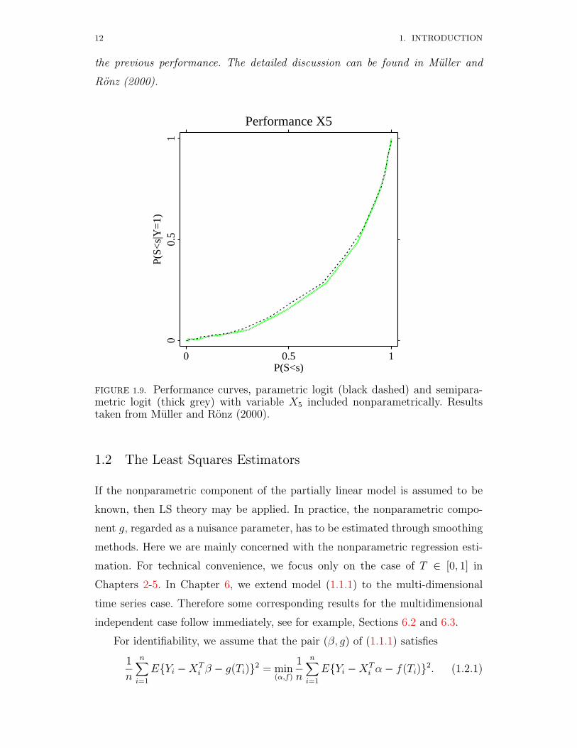
maximum–likelihood. Figure 1.9 compares the performance of the parametric logit
fit and the semiparametric logit fit obtained by including X5 in a nonparametric
way. Their analysis indicated that this generalized partially linear model improves
12 1. INTRODUCTION
the previous performance. The detailed discussion can be found in Muller and
Ronz (2000).
Performance X5
0 0.5 1P(S<s)
00.
51
P(S<
s|Y
=1)
FIGURE 1.9. Performance curves, parametric logit (black dashed) and semipara-metric logit (thick grey) with variable X5 included nonparametrically. Resultstaken from Muller and Ronz (2000).
1.2 The Least Squares Estimators
If the nonparametric component of the partially linear model is assumed to be
known, then LS theory may be applied. In practice, the nonparametric compo-
nent g, regarded as a nuisance parameter, has to be estimated through smoothing
methods. Here we are mainly concerned with the nonparametric regression esti-
mation. For technical convenience, we focus only on the case of T ∈ [0, 1] in
Chapters 2-5. In Chapter 6, we extend model (1.1.1) to the multi-dimensional
time series case. Therefore some corresponding results for the multidimensional
independent case follow immediately, see for example, Sections 6.2 and 6.3.
For identifiability, we assume that the pair (β, g) of (1.1.1) satisfies
1
n
n∑i=1
EYi −XTi β − g(Ti)2 = min
(α,f)
1
n
n∑i=1
EYi −XTi α− f(Ti)2. (1.2.1)

1. INTRODUCTION 13
This implies that if XTi β1 +g1(Ti) = XT
i β2 +g2(Ti) for all 1 ≤ i ≤ n, then β1 = β2
and g1 = g2 simultaneously. We will justify this separately for the random design
case and the fixed design case.
For the random design case, if we assume that E[Yi|(Xi, Ti)] = XTi β1 +
g1(Ti) = XTi β2 + g2(Ti) for all 1 ≤ i ≤ n, then it follows from EYi − XT
i β1 −g1(Ti)2 = EYi−XT
i β2−g2(Ti)2+(β1−β2)TE(Xi−E[Xi|Ti])(Xi−E[Xi|Ti])T(β1 − β2) that we have β1 = β2 due to the fact that the matrix E(Xi −E[Xi|Ti])(Xi − E[Xi|Ti])T is positive definite assumed in Assumption 1.3.1(i)
below. Thus g1 = g2 follows from the fact gj(Ti) = E[Yi|Ti] − E[XTi βj|Ti] for all
1 ≤ i ≤ n and j = 1, 2.
For the fixed design case, we can justify the identifiability using several dif-
ferent methods. We here provide one of them. Suppose that g of (1.1.1) can be
parameterized as G = g(T1), . . . , g(Tn)T = Wγ used in (1.2.2), where γ is a
vector of unknown parameters.
Then submitting G = Wγ into (1.2.1), we have the normal equations
XTXβ = XT (Y −Wγ) and Wγ = P (Y −Xβ),
where P = W (W TW )−1W T , XT = (X1, . . . , Xn) and Y T = (Y1, . . . , Yn).
Similarly, if we assume that E[Yi] = XTi β1 + g1(Ti) = XT
i β2 + g2(Ti) for all
1 ≤ i ≤ n, then it follows from Assumption 1.3.1(ii) below and the fact that
1/nE(Y −Xβ1 −Wγ1)T (Y −Xβ1 −Wγ1) = 1/nE(Y −Xβ2 −Wγ2)T (Y −Xβ2 −Wγ2) + 1/n(β1 − β2)TXT (I − P )X(β1 − β2) that we have β1 = β2 and
g1 = g2 simultaneously.
Assume that (Xi, Ti, Yi); i = 1, . . . , n. satisfies model (1.1.1). Let ωni(t)=ωni(t; T1, . . . , Tn) be positive weight functions depending on t and the design
points T1, . . . , Tn. For every given β, we define an estimator of g(·) by
gn(t; β) =n∑i=1
ωnj(t)(Yi −XTi β).
We often drop the β for convenience. Replacing g(Ti) by gn(Ti) in model (1.1.1)
and using the LS criterion, we obtain the least squares estimator of β:
βLS = (XT X)−1XT Y, (1.2.2)
which is just the estimator βGJS in (1.1.4) with a different smoothing operator.

14 1. INTRODUCTION
The nonparametric estimator of g(t) is then defined as follows:
gn(t) =n∑i=1
ωni(t)(Yi −XTi βLS). (1.2.3)
where XT = (X1, . . . , Xn) with Xj = Xj−∑ni=1 ωni(Tj)Xi and YT = (Y1, . . . , Yn)
with Yj = Yj −∑ni=1 ωni(Tj)Yi. Due to Lemma A.2 below, we have as n → ∞
n−1(XT X)→ Σ, where Σ is a positive matrix. Thus, we assume that n(XT X)−1
exists for large enough n throughout this monograph.
When ε1, . . . , εn are identically distributed, we denote their distribution func-
tion by ϕ(·) and the variance by σ2, and define the estimator of σ2 by
σ2n =
1
n
n∑i=1
(Yi − XTi βLS)2 (1.2.4)
In this monograph, most of the estimation procedures are based on the estimators
(1.2.2), (1.2.3) and (1.2.4).
1.3 Assumptions and Remarks
This monograph considers the two cases: the fixed design and the i.i.d. random
design. When considering the random case, denote
hj(Ti) = E(xij|Ti) and uij = xij − E(xij|Ti).
Assumption 1.3.1 i) sup0≤t≤1 E(‖X1‖3|T = t) < ∞ and Σ = CovX1 −E(X1|T1) is a positive definite matrix. The random errors εi are independent
of (Xi, Ti).
ii) When (Xi, Ti) are fixed design points, there exist continuous functions
hj(·) defined on [0, 1] such that each component of Xi satisfies
xij = hj(Ti) + uij 1 ≤ i ≤ n, 1 ≤ j ≤ p (1.3.1)
where uij is a sequence of real numbers satisfying
limn→∞
1
n
n∑i=1
uiuTi = Σ (1.3.2)
and for m = 1, . . . , p,
lim supn→∞
1
anmax
1≤k≤n
∣∣∣∣∣k∑i=1
ujim
∣∣∣∣∣ <∞ (1.3.3)
for all permutations (j1, . . . , jn) of (1, 2, . . . , n), where ui = (ui1, . . . , uip)T , an =
n1/2 log n, and Σ is a positive definite matrix.

1. INTRODUCTION 15
Throughout the monograph, we apply Assumption 1.3.1 i) to the case of
random design points and Assumption 1.3.1 ii) to the case where (Xi, Ti) are
fixed design points. Assumption 1.3.1 i) is a reasonable condition for the
random design case, while Assumption 1.3.1 ii) generalizes the corresponding
conditions of Heckman (1986) and Rice (1986), and simplifies the conditions of
Speckman (1988). See also Remark 2.1 (i) of Gao and Liang (1997).
Assumption 1.3.2 The first two derivatives of g(·) and hj(·) are Lipschitz
continuous of order one.
Assumption 1.3.3 When (Xi, Ti) are fixed design points, the positive weight
functions ωni(·) satisfy
(i) max1≤i≤n
n∑j=1
ωni(Tj) = O(1),
max1≤j≤n
n∑i=1
ωni(Tj) = O(1),
(ii) max1≤i,j≤n
ωni(Tj) = O(bn),
(iii) max1≤i≤n
n∑j=1
ωnj(Ti)I(|Ti − Tj| > cn) = O(cn),
where bn and cn are two sequences satisfying lim supn→∞
nb2n log4 n <∞, lim inf
n→∞nc2
n >
0, lim supn→∞
nc4n log n <∞ and lim sup
n→∞nb2
nc2n <∞. When (Xi, Ti) are i.i.d. random
design points, (i), (ii) and (iii) hold with probability one.
Remark 1.3.1 There are many weight functions satisfying Assumption 1.3.3.
For examples,
W(1)ni (t) =
1
hn
∫ Si
Si−1
K(t− sHn
)ds, W
(2)ni (t) = K
(t− TiHn
)/ n∑j=1
K(t− TjHn
),
where Si = 12(T(i) + T(i−1)), i = 1, · · · , n − 1, S0 = 0, Sn = 1, and T(i) are the
order statistics of Ti. K(·) is a kernel function satisfying certain conditions,
and Hn is a positive number sequence. Here Hn = hn or rn, hn is a bandwidth
parameter, and rn = rn(t, T1, · · · , Tn) is the distance from t to the kn−th nearest
neighbor among the T ′i s, and where kn is an integer sequence.
We can justify that both W(1)ni (t) and W
(2)ni (t) satisfy Assumption 1.3.3. The
details of the justification are very lengthy and omitted. We also want to point

16 1. INTRODUCTION
out that when ωni is either W(1)ni or W
(2)ni , Assumption 1.3.3 holds automatically
with Hn = λn−1/5 for some 0 < λ <∞. This is the same as the result established
by Speckman (1988) (see Theorem 2 with ν = 2), who pointed out that the usual
n−1/5 rate for the bandwidth is fast enough to establish that the LS estimate βLS
of β is√n-consistent. Sections 2.1.3 and 6.4 will discuss some practical selections
for the bandwidth.
Remark 1.3.2 Throughout this monograph, we are mostly using Assumption
1.3.1 ii) and 1.3.3 for the fixed design case. As a matter of fact, we can replace
Assumption 1.3.1 ii) and 1.3.3 by the following corresponding conditions.
Assumption 1.3.1 ii)’ When (Xi, Ti) are the fixed design points, equations
(1.3.1) and (1.3.2) hold.
Assumption 1.3.3’ When (Xi, Ti) are fixed design points, Assumption 1.3.3
(i)-(iii) holds. In addition, the weight functions ωni satisfy
(iv) max1≤i≤n
n∑j=1
ωnj(Ti)ujl = O(dn),
(v)1
n
n∑j=1
fjujl = O(dn),
(vi)1
n
n∑j=1
n∑k=1
ωnk(Tj)uksujl = O(dn)
for all 1 ≤ l, s ≤ p, where dn is a sequence of real numbers satisfying lim supn→∞
nd4n
log n <∞, fj = f(Tj)−∑nk=1 ωnk(Tj)f(Tk) for f = g or hj defined in (1.3.1).
Obviously, the three conditions (iv), (v) and (vi) follows from (1.3.3) and
Abel’s inequality.
When the weight functions ωni are chosen as W(2)ni defined in Remark 1.3.1,
Assumptions 1.3.1 ii)’ and 1.3.3’ are almost the same as Assumptions (a)-(f) of
Speckman (1988). As mentioned above, however, we prefer to use Assumptions
1.3.1 ii) and 1.3.3 for the fixed design case throughout this monograph.
Under the above assumptions, we provide bounds for hj(Ti)−∑nk=1 ωnk(Ti)
hj(Tk) and g(Ti)−∑nk=1 ωnk(Ti)g(Tk) in the appendix.
1.4 The Scope of the Monograph
The main objectives of this monograph are: (i) To present a number of theoreti-
cal results for the estimators of both parametric and nonparametric components,

1. INTRODUCTION 17
and (ii) To illustrate the proposed estimation and testing procedures by several
simulated and true data sets using XploRe-The Interactive Statistical Comput-
ing Environment (see Hardle, Klinke and Muller, 1999), available on website:
http://www.xplore-stat.de.
In addition, we generalize the existing approaches for homoscedasticity to
heteroscedastic models, introduce and study partially linear errors-in-variables
models, and discuss partially linear time series models.
1.5 The Structure of the Monograph
The monograph is organized as follows: Chapter 2 considers a simple partially
linear model. An estimation procedure for the parametric component of the par-
tially linear model is established based on the nonparametric weight sum. Section
2.1 mainly provides asymptotic theory and an estimation procedure for the para-
metric component with heteroscedastic errors. In this section, the least squares
estimator βLS of (1.2.2) is modified to the weighted least squares estimator βWLS.
For constructing βWLS, we employ the split-sample techniques. The asymp-
totic normality of βWLS is then derived. Three different variance functions are
discussed and estimated. The selection of smoothing parameters involved in the
nonparametric weight sum is also discussed in Subsection 2.1.3. Simulation com-
parison is also implemented in Subsection 2.1.4. A modified estimation procedure
for the case of censored data is given in Section 2.2. Based on a modification of
the Kaplan-Meier estimator, synthetic data and an estimator of β are con-
structed. We then establish the asymptotic normality for the resulting estimator
of β. We also examine the behaviors of the finite sample through a simulated
example. Bootstrap approximations are given in Section 2.3.
Chapter 3 discusses the estimation of the nonparametric component without
the restriction of constant variance. Convergence and asymptotic normality of the
nonparametric estimate are given in Sections 3.2 and 3.3. The estimation methods
proposed in this chapter are illustrated through examples in Section 3.4, in which
the estimator (1.2.3) is applied to the analysis of the logarithm of the earnings
to labour market experience.
In Chapter 4, we consider both linear and nonlinear variables with measure-
ment errors. An estimation procedure and asymptotic theory for the case where

18 1. INTRODUCTION
the linear variables are measured with measurement errors are given in Section
4.1. The common estimator given in (1.2.2) is modified by applying the so-called
“correction for attenuation”, and hence deletes the inconsistence caused by
measurement error. The modified estimator is still asymptotically normal as
(1.2.2) but with a more complicated form of the asymptotic variance. Section 4.2
discusses the case where the nonlinear variables are measured with measurement
errors. Our conclusion shows that asymptotic normality heavily depends on the
distribution of the measurement error when T is measured with error. Examples
and numerical discussions are presented to support the theoretical results.
Chapter 5 discusses several relatively theoretic topics. The laws of the
iterative logarithm (LIL) and the Berry-Esseen bounds for the parametric
component are established. Section 5.3 constructs a class of asymptotically
efficient estimators of β. Two classes of efficiency concepts are introduced.
The well-known Bahadur asymptotic efficiency, which considers the exponential
rate of the tail probability, and second order asymptotic efficiency are dis-
cussed in detail in Sections 5.4 and 5.5, respectively. The results of this chapter
show that the LS estimate can be modified to have both Bahadur asymptotic
efficiency and second order asymptotic efficiency even when the parametric and
nonparametric components are dependent. The estimation of the error distribu-
tion is also investigated in Section 5.6.
Chapter 6 generalizes the case studied in previous chapters to partially
linear time series models and establishes asymptotic results as well as small
sample studies. At first we present several data-based test statistics to deter-
mine which model should be chosen to model a partially linear dynamical system.
Secondly we propose a cross-validation (CV) based criterion to select the optimum
linear subset for a partially linear regression model. We investigate the problem
of selecting the optimum bandwidth for a partially linear autoregressive
model. Finally, we summarize recent developments in a general class of additive
stochastic regression models.

2ESTIMATION OF THE PARAMETRICCOMPONENT
2.1 Estimation with Heteroscedastic Errors
2.1.1 Introduction
This section considers asymptotic normality for the estimator of β when ε is a
homoscedastic error. This aspect has been discussed by Chen (1988), Robinson
(1988), Speckman (1988), Hong (1991), Gao and Zhao (1993), Gao, Chen and
Zhao (1994) and Gao, Hong and Liang (1995). Here we state one of the main
results obtained by Gao, Hong and Liang (1995) for model (1.1.1).
Theorem 2.1.1 Under Assumptions 1.3.1-1.3.3, βLS is an asymptotically nor-
mal estimator of β, i.e.,
√n(βLS − β) −→L N(0, σ2Σ−1). (2.1.1)
Furthermore, assume that the weight functions ωni(t) are Lipschitz continuous
of order one. Let supiE|εi|3 <∞, bn = n−4/5 log−1/5 n and cn = n−2/5 log2/5 n in
Assumption 1.3.3. Then with probability one
sup0≤t≤1
|gn(t)− g(t)| = O(n−2/5 log2/5 n). (2.1.2)
The proof of this theorem has been given in several papers. The proof of
(2.1.1) is similar to that of Theorem 2.1.2 below. Similar to the proof of Theorem
5.1 of Muller and Stadtmuller (1987), the proof of (2.1.2) can be completed. The
details have been given in Gao, Hong and Liang (1995).
Example 2.1.1 Suppose the data are drawn from Yi = XTi β0 + T 3
i + εi for
i = 1, . . . , 100, where β0 = (1.2, 1.3, 1.4)T , Ti ∼ U [0, 1], εi ∼ N(0, 0.01) and Xi ∼
N(0,Σx) with Σx =
0.81 0.1 0.20.1 2.25 0.10.2 0.1 1
. In this simulation, we perform 20 repli-
cations and take bandwidth 0.05. The estimate βLS is (1.201167, 1.30077, 1.39774)T
with mean squared error (2.1 ∗ 10−5, 2.23 ∗ 10−5, 5.1 ∗ 10−5)T . The estimate of
g0(t)(= t3) is based on (1.2.3). For comparison, we also calculate a parametric

20 2. ESTIMATION OF THE PARAMETRIC COMPONENT
fit for g0(t). Figure 2.1 shows the parametric estimate and nonparametric fitting
for g0(t). The true curve is given by grey line(in the left side), the nonparametric
estimate by thick curve(in the right side) and the parametric estimate by the black
straight line.
Simulation comparison
00.
5g(
T)
and
its p
aram
etri
c es
timat
es
Simulation comparison
00.
20.
40.
60.
8pa
ram
etri
c an
d no
npar
amet
ric
estim
ates
FIGURE 2.1. Parametric and nonparametric estimates of the function g(T )
Schick (1996b) considered the problem of heteroscedasticity, i.e., non-
constant variance, for model (1.1.1). He constructed root-n consistent weighted
least squares estimates for the case where the variance is known up to a
multiplicative constant. In his discussion, he assumed that the nonconstant vari-
ance function of Y given (X,T ) is an unknown smooth function of an exogenous
random vector W .
In the remainder of this section, we mainly consider model (1.1.1) with
heteroscedastic error and focus on the following cases: (i) σ2i is an unknown
function of independent exogenous variables; (ii) σ2i is an unknown function of
Ti; and (iii) σ2i is an unknown function of XT
i β+g(Ti). We establish asymptotic
results for the three cases. In relation to our results, we mention recent develop-
ments in linear and nonparametric regression models with heteroscedastic er-
rors. See for example, Bickel (1978), Box and Hill (1974), Carroll (1982), Carroll

2. ESTIMATION OF THE PARAMETRIC COMPONENT 21
and Ruppert (1982), Carroll and Hardle (1989), Fuller and Rao (1978), Hall and
Carroll (1989), Jobson and Fuller (1980), Mak (1992) and Muller and Stadtmuller
(1987).
Let (Yi, Xi, Ti), i = 1, . . . , n denote a sequence of random samples from
Yi = XTi β + g(Ti) + σiξi, i = 1, . . . , n, (2.1.3)
where (Xi, Ti) are i.i.d. random variables, ξi are i.i.d. with mean 0 and variance
1, and σ2i are some functions of other variables. The concrete forms of σ2
i will be
discussed in later subsections.
When the errors are heteroscedastic, βLS is modified to a weighted least
squares estimator
βW =( n∑i=1
γiXiXTi
)−1( n∑i=1
γiXiYi)
(2.1.4)
for some weights γi i = 1, . . . , n. In this section, we assume that γi is either a
sequence of random variables or a sequence of constants. In our model (2.1.3) we
take γi = 1/σ2i .
In principle the weights γi (or σ2i ) are unknown and must be estimated. Let
γi, i = 1, . . . , n be a sequence of estimators of γi. We define an estimator of
β by substituting γi in (2.1.4) by γi.
In order to develop the asymptotic theory conveniently, we use the tech-
nique of split-sample. Let kn(≤ n/2) be the largest integer part of n/2. γ(1)i
and γ(2)i are the estimators of γi based on the first kn observations (X1, T1, Y1),
. . . , (Xkn , Tkn , Ykn), and the later n − kn observations (Xkn+1, Tkn+1, Ykn+1), . . . ,
(Xn, Tn, Yn), respectively. Define
βWLS =( n∑i=1
γiXiXTi
)−1( kn∑i=1
γ(2)i XiYi +
n∑i=kn+1
γ(1)i XiYi
)(2.1.5)
as the estimator of β.
The next step is to prove that βWLS is asymptotically normal. We first prove
that βW is asymptotically normal, and then show that√n(βWLS−βW ) converges
to zero in probability.
Assumption 2.1.1 sup0≤t≤1 E(‖X1‖3|T = t) < ∞. When γi is a sequence of
real numbers, then limn→∞ 1/n∑ni=1 γiuiu
Ti = B, where B is a positive definite
matrix, and limn→∞ 1/n∑ni=1 γi < ∞. When γi is a sequence of i.i.d. random
variables, then B = E(γ1u1uT1 ) is a positive definite matrix.

22 2. ESTIMATION OF THE PARAMETRIC COMPONENT
Assumption 2.1.2 There exist constants C1 and C2 such that
0 < C1 ≤ mini≤n
γi ≤ maxi≤n
γi < C2 <∞.
We suppose that the estimator γi of γi satisfy
max1≤i≤n
|γi − γi| = oP (n−q) q ≥ 1/4. (2.1.6)
We shall construct estimators to satisfy (2.1.6) for three kinds of γi later. The
following theorems present general results for the estimators of the parametric
components in the partially linear heteroscedastic model (2.1.3).
Theorem 2.1.2 Assume that Assumptions 2.1.1, 2.1.2 and 1.3.2-1.3.3 hold. Then
βW is an asymptotically normal estimator of β, i.e.,
√n(βW − β) −→L N(0, B−1ΣB−1).
Theorem 2.1.3 Under Assumptions 2.1.1, 2.1.2 and (2.1.6), βWLS is asymp-
totically equivalent to βW , i.e.,√n(βWLS − β) and
√n(βW − β) have the same
asymptotically normal distribution.
Remark 2.1.1 In the case of constant error variance, i.e. σ2i ≡ σ2, Theorem
2.1.2 has been obtained by many authors. See, for example, Theorem 2.1.1.
Remark 2.1.2 Theorem 2.1.3 not only assures that our estimator given in (2.1.5)
is asymptotically equivalent to the weighted LS estimator with known weights,
but also generalizes the results obtained previously.
Before proving Theorems 2.1.2 and 2.1.3, we discuss three different variance
functions and construct their corresponding estimates. Subsection 2.1.4 gives
small sample simulation results. The proofs of Theorems 2.1.2 and 2.1.3 are post-
poned to Subsection 2.1.5.
2.1.2 Estimation of the Non-constant Variance Functions
2.1.2.1 Variance is a Function of Exogenous Variables

2. ESTIMATION OF THE PARAMETRIC COMPONENT 23
This subsection is devoted to the nonparametric heteroscedasticity structure
σ2i = H(Wi),
where H is unknown and Lipschitz continuous, Wi; i = 1, . . . , n is a se-
quence of i.i.d. design points defined on [0, 1], which are assumed to be indepen-
dent of (ξi, Xi, Ti).
Define
Hn(w) =n∑j=1
ωnj(w)Yj −XTj βLS − gn(Ti)2
as the estimator of H(w), where ωnj(t); j = 1, . . . , n is a sequence of weight
functions satisfying Assumption 1.3.3 with ωnj replaced by ωnj.
Theorem 2.1.4 Assume that the conditions of Theorem 2.1.2 hold. Let cn =
n−1/3 log n in Assumption 1.3.3. Then
sup1≤i≤n
|Hn(Wi)−H(Wi)| = OP (n−1/3 log n).
Proof. Note that
Hn(Wi) =n∑j=1
ωnj(Wi)(Yj − XTj βLS)2
=n∑j=1
ωnj(Wi)XTj (β − βLS) + g(Ti) + εi2
= (β − βLS)Tn∑j=1
ωnj(Wi)XjXTj (β − βLS) +
n∑j=1
ωnj(Wi)g2(Ti)
+n∑j=1
ωnj(Wi)ε2i + 2
n∑j=1
ωnj(Wi)XTj (β − βLS)g(Ti)
+2n∑j=1
ωnj(Wi)XTj (β − βLS)εi + 2
n∑j=1
ωnj(Wi)g(Ti)εi. (2.1.7)
The first term of (2.1.7) is therefore OP (n−2/3) since∑nj=1 XjX
Tj is a symmetric
matrix, 0 < ωnj(Wi) ≤ Cn−2/3,
n∑j=1
ωnj(Wi)− Cn−2/3XjXTj
is a p × p nonpositive matrix, and βLS − β = OP (n−1/2). The second term of
(2.1.7) is easily shown to be of order OP (n1/3c2n).

24 2. ESTIMATION OF THE PARAMETRIC COMPONENT
Now we need to prove
supi
∣∣∣ n∑j=1
ωnj(Wi)ε2i −H(Wi)
∣∣∣ = OP (n−1/3 log n), (2.1.8)
which is equivalent to proving the following three results
supi
∣∣∣ n∑j=1
ωnj(Wi) n∑k=1
ωnk(Tj)εk2∣∣∣ = OP (n−1/3 log n), (2.1.9)
supi
∣∣∣ n∑j=1
ωnj(Wi)ε2i −H(Wi)
∣∣∣ = OP (n−1/3 log n), (2.1.10)
supi
∣∣∣ n∑j=1
ωnj(Wi)εj n∑k=1
ωnk(Tj)εk∣∣∣ = OP (n−1/3 log n). (2.1.11)
(A.3) below assures that (2.1.9) holds. Lipschitz continuity of H(·) and as-
sumptions on ωnj(·) imply that
supi
∣∣∣ n∑j=1
ωnj(Wi)ε2i −H(Wi)
∣∣∣ = OP (n−1/3 log n). (2.1.12)
By taking aki = ωnk(Wi)H(Wk), Vk = ξ2k − 1 r = 2, p1 = 2/3 and p2 = 0 in
Lemma A.3, we have
supi
∣∣∣ n∑j=1
ωnj(Wi)H(Wj)(ξ2j − 1)
∣∣∣ = OP (n−1/3 log n). (2.1.13)
A combination of (2.1.13) and (2.1.12) implies (2.1.10). Cauchy-Schwarz inequal-
ity, (2.1.9) and (2.1.10) imply (2.1.11), and then (2.1.8). The last three terms of
(2.1.7) are all of order OP (n−1/3 log n) by Cauchy-Schwarz inequality. We there-
fore complete the proof of Theorem 2.1.4.
2.1.2.2 Variance is a Function of the Design Points Ti
In this subsection we consider the case where σ2i is a function of Ti, i.e.,
σ2i = H(Ti), H unknown Lipschitz continuous.
Similar to Subsection 2.1.2.1, we define our estimator of H(·) as
Hn(t) =n∑j=1
ωnj(t)Yj −XTj βLS − gn(Ti)2.

2. ESTIMATION OF THE PARAMETRIC COMPONENT 25
Theorem 2.1.5 Under the conditions of Theorem 2.1.2, we have
sup1≤i≤n
|Hn(Ti)−H(Ti)| = OP (n−1/3 log n).
Proof. The proof of Theorem 2.1.5 is similar to that of Theorem 2.1.4 and there-
fore omitted.
2.1.2.3 Variance is a Function of the Mean
Here we consider model (2.1.3) with
σ2i = HXT
i β + g(Ti), H unknown Lipschitz continuous.
This means that the variance is an unknown function of the mean response.
Several related situations in linear and nonlinear models have been discussed by
Box and Hill (1974), Bickel (1978), Jobson and Fuller (1980), Carroll (1982) and
Carroll and Ruppert (1982).
Since H(·) is assumed to be completely unknown, the standard method is
to get information about H(·) by replication, i.e., to consider the following
“improved” partially linear heteroscedastic model
Yij = XTi β + g(Ti) + σiξij, j = 1, . . . ,mi; i = 1, . . . , n,
where Yij is the response of the j−th replicate at the design point (Xi, Ti), ξij
are i.i.d. with mean 0 and variance 1, β, g(·) and (Xi, Ti) are as defined in (2.1.3).
We here apply the idea of Fuller and Rao (1978) for linear heteroscedastic
model to construct an estimate of σ2i . Based on the least squares estimate βLS
and the nonparametric estimate gn(Ti), we use Yij − XTi βLS + gn(Ti) to define
σ2i =
1
mi
mi∑j=1
[Yij − XTi βLS + gn(Ti)]2, (2.1.14)
with a positive sequence mi; i = 1, · · · , n determined later.
Theorem 2.1.6 Let mi = ann2q def
= m(n) for some sequence an converging to
infinity. Suppose the conditions of Theorem 2.1.2 hold. Then
sup1≤i≤n
|σ2i −HXT
i β + g(Ti)| = oP (n−q) q ≥ 1/4.
26 2. ESTIMATION OF THE PARAMETRIC COMPONENT
Proof. We provide only an outline for the proof of Theorem 2.1.6. Obviously
|σ2i −HXT
i β + g(Ti)| ≤ 3XTi (β − βLS)2 + 3g(Ti)− gn(Ti)2
+3
mi
mi∑j=1
σ2i (ξ
2ij − 1).
The first two items are obviously oP (n−q). Since ξij are i.i.d. with mean zero and
variance 1, by taking mi = ann2q, using the law of the iterated logarithm and the
boundedness of H(·), we have
1
mi
mi∑j=1
σ2i (ξ
2ij − 1) = Om(n)−1/2 logm(n) = oP (n−q).
Thus we derive the proof of Theorem 2.1.6.
2.1.3 Selection of Smoothing Parameters
In practice, an important problem is how to select the smoothing parameter
involved in the weight functions ωni. Currently, the results on bandwidth selec-
tion for completely nonparametric regression can be found in the monographs by
Eubank (1988), Hardle (1990, 1991), Wand and Jones (1994), Fan and Gijbels
(1996), and Bowman and Azzalini (1997).
More recently, Gao and Anh (1999) considered the selection of an optimum
truncation parameter for model (1.1.1) and established large and small sample
results for the case where the weight functions ωni are a sequence of orthogonal
series. See also Gao (1998), who discussed the time series case and provided both
theory and practical applications.
In this subsection, we briefly mention the selection procedure for bandwidth
for the case where the weight function is a kernel weight.
For 1 ≤ i ≤ n, define
ωi,n(t) = K(t− Ti
h
)/ n∑j=1,j 6=i
K(t− Tj
h
),
gi,n(t, β) =n∑
j=1,j 6=iωj,n(t)(Yj −XT
j β).
We now define the modified LS estimator β(h) of β by minimizing
n∑i=1
Yi −XTi β − gi,n(Ti, β)2.

2. ESTIMATION OF THE PARAMETRIC COMPONENT 27
The Cross-Validation (CV) function can be defined as
CV (h) =1
n
n∑i=1
Yi −XTi β(h)− gi,n(Ti, β(h))2.
Let h denote the estimator of h, which is obtained by minimizing the CV function
CV(h) over h ∈ Θh, where Θh is an interval defined by
Θh = [λ1n−1/5−η1 , λ2n
−1/5+η1 ],
where 0 < λ1 < λ2 < ∞ and 0 < η1 < 1/20 are constants. Under Assumptions
1.3.1-1.3.3, we can show that the CV function provides an optimum bandwidth
for estimating both β and g. Details for the i.i.d. case are similar to those in
Section 6.4.
2.1.4 Simulation Comparisons
We present a small simulation study to illustrate the properties of the theoretical
results in this chapter. We consider the following model with different variance
functions.
Yi = XTi β + g(Ti) + σiεi, i = 1, . . . , n = 300,
where εi is a sequence of the standard normal random variables, Xi and Tiare mutually independent uniform random variables on [0, 1], β = (1, 0.75)T and
g(t) = sin(t). The number of simulations for each situation is 500.
Three models for the variance functions are considered. LSE and WLSE rep-
resent the least squares estimator and the weighted least squares estimator
given in (1.1.1) and (2.1.5), respectively.
• Model 1: σ2i = T 2
i ;
• Model 2: σ2i = W 3
i ; where Wi are i.i.d. uniformly distributed random vari-
ables.
• Model 3: σ2i = a1 exp[a2XT
i β + g(Ti)2], where (a1, a2) = (1/4, 1/3200).
The case where g ≡ 0 has been studied by Carroll (1982).
From Table 2.1, one can find that our estimator (WLSE) is better than LSE
in the sense of both bias and MSE for each of the models.

28 2. ESTIMATION OF THE PARAMETRIC COMPONENT
TABLE 2.1. Simulation results (×10−3)
Estimator Variance β0 = 1 β1 = 0.75Model Bias MSE Bias MSE
LSE 1 8.696 8.7291 23.401 9.1567WLSE 1 4.230 2.2592 1.93 2.0011LSE 2 12.882 7.2312 5.595 8.4213
WLSE 2 5.676 1.9235 0.357 1.3241LSE 3 5.9 4.351 18.83 8.521
WLSE 3 1.87 1.762 3.94 2.642
By the way, we also study the behavior of the estimate for the nonparametric
part g(t)
n∑i=1
ω∗ni(t)(Yi − XTi βWLS),
where ω∗ni(·) are weight functions satisfying Assumption 1.3.3. In simulation,
we take Nadaraya-Watson weight function with quartic kernel(15/16)(1 −u2)2I(|u| ≤ 1) and use the cross-validation criterion to select the bandwidth.
Figure 2.2 presents for the simulation results of the nonparametric parts of models
1–3, respectively. In the three pictures, thin dashed lines stand for true values and
thick solid lines for our estimate values. The figures indicate that our estimators
for the nonparametric part perform also well except in the neighborhoods of the
points 0 and 1.
2.1.5 Technical Details
We introduce the following notation,
An =n∑i=1
γiXiXTi , An =
n∑i=1
γiXiXTi .
Proof of Theorem 2.1.2. It follows from the definition of βW that
βW − β = A−1n
n∑i=1
γiXig(Ti) +n∑i=1
γiXiεi.
We will complete the proof by proving the following three facts for j = 1, . . . , p,
(i) H1j = 1/√n∑ni=1 γixij g(Ti) = oP (1);
(ii) H2j = 1/√n∑ni=1 γixij
∑nk=1 ωnk(Ti)ξk
= oP (1);

2. ESTIMATION OF THE PARAMETRIC COMPONENT 29
The first model
0 0.5 1
T (a)
00.
51
g(T)
and
its es
timat
e val
ues
The third model
0 0.5 1
T (c)
00.
51
g(T)
and
its es
timat
e val
ues
The second model
0 0.5 1
T (b)
00.
51
g(T)
and
its es
timat
e val
ues
FIGURE 2.2. Estimates of the function g(T ) for the three models
(iii) H3 = 1/√n∑ni=1 γiXiξi −→L N(0, B−1ΣB−1).
The proof of (i) is mainly based on Lemmas A.1 and A.3. Observe that
√nH1j =
n∑i=1
γiuij gi +n∑i=1
γihnij gi −n∑i=1
γin∑q=1
ωnq(Ti)uqj gi, (2.1.15)
where hnij = hj(Ti)−∑nk=1 ωnk(Ti)hj(Tk). In Lemma A.3, we take r = 2, Vk = ukl,
aji = gj, 1/4 < p1 < 1/3 and p2 = 1− p1. Then, the first term of (2.1.15) is
OP (n−(2p1−1)/2) = oP (n1/2).
The second term of (2.1.15) can be easily shown to be order OP (nc2n) by using
Lemma A.1.
The proof of the third term of (2.1.15) follows from Lemmas A.1 and A.3,
and ∣∣∣ n∑i=1
n∑q=1
γiωnq(Ti)uqj gi∣∣∣ ≤ C2nmax
i≤n|gi|max
i≤n
∣∣∣ n∑q=1
ωnq(Ti)uqj∣∣∣
= O(n2/3cn log n) = op(n1/2).
Thus we complete the proof of (i).

30 2. ESTIMATION OF THE PARAMETRIC COMPONENT
We now show (ii), i.e.,√nH2j → 0. Notice that
√nH2j =
n∑i=1
γi n∑k=1
xkjωni(Tk)ξi
=n∑i=1
γi n∑k=1
ukjωni(Tk)ξi +
n∑i=1
γi n∑k=1
hnkjωni(Tk)ξi
−n∑i=1
γi[ n∑k=1
n∑q=1
uqjωnq(Tk)ωni(Tk)
]ξi. (2.1.16)
The order of the first term of (2.1.16) is O(n−(2p1−1)/2 log n) by letting r = 2,
Vk = ξk, ali =∑nk=1 ukjωni(Tk), 1/4 < p1 < 1/3 and p2 = 1− p1 in Lemma A.3.
It follows from Lemma A.1 and (A.3) that the second term of (2.1.16) is
bounded by
∣∣∣ n∑i=1
γi n∑k=1
hnkjωni(Tk)ξi∣∣∣ ≤ nmax
k≤n
∣∣∣ n∑i=1
ωni(Tk)ξi∣∣∣maxj,k≤n
|hnkj|
= O(n2/3cn log n) a.s. (2.1.17)
The same argument as that for (2.1.17) yields that the third term of (2.1.16) is
bounded by
∣∣∣ n∑k=1
n∑i=1
γiωni(Tk)ξi n∑
q=1
uqjωnq(Tk)∣∣∣
≤ nmaxk≤n
∣∣∣ n∑i=1
ωni(Tk)ξi∣∣∣×max
k≤n
∣∣∣ k∑q=1
uqjωnq(Tj)∣∣∣
= OP (n1/3 log2 n) = oP (n1/2). (2.1.18)
A combination (2.1.16)–(2.1.18) implies (ii).
Using the same procedure as in Lemma A.2, we deduce that
limn→∞
1
n
n∑i=1
γiXTi Xi = B. (2.1.19)
A central limit theorem shows that as n→∞
1√n
n∑i=1
γiXiξi −→L N(0,Σ).
We therefore show that as n→∞
1√nA−1n
n∑i=1
γiXiξi −→L N(0, B−1ΣB−1).
This completes the proof of Theorem 2.1.2.

2. ESTIMATION OF THE PARAMETRIC COMPONENT 31
Proof of Theorem 2.1.3. In order to complete the proof of Theorem 2.1.3, we
only need to prove
√n(βWLS − βW ) = oP (1).
First we state a fact, whose proof is immediately derived by (2.1.6) and (2.1.19),
1
n|an(j, l)− an(j, l)| = oP (n−q) (2.1.20)
for j, l = 1, . . . , p, where an(j, l) and an(j, l) are the (j, l)−th elements of An and
An, respectively. The fact (2.1.20) will be often used later.
It follows that
βWLS − βW =1
2
A−1n (An − An)A−1
n
n∑i=1
γiXig(Ti)
+A−1n
kn∑i=1
(γi − γ(2)i )Xig(Ti) + A−1
n (An − An)A−1n
n∑i=1
γiXiξi
+A−1n
kn∑i=1
(γi − γ(2)i )Xiξi + A−1
n
n∑i=kn+1
(γi − γ(1)i )Xig(Ti)
+A−1n
n∑i=kn+1
(γi − γ(1)i )Xiξi
. (2.1.21)
By Cauchy-Schwarz inequality, for any j = 1, . . . , p,∣∣∣ n∑i=1
γixij g(Ti)∣∣∣ ≤ C
√nmax
i≤n|g(Ti)|
( n∑i=1
x2ij
)1/2,
which is oP (n3/4) by Lemma A.1 and (2.1.19). Thus each element of the first term
of (2.1.21) is oP (n−1/2) by using the fact that each element of A−1n (An − An)A−1
n
is oP (n−5/4). The similar argument demonstrates that each element of the second
and fifth terms is also oP (n−1/2).
Similar to the proof of H2j = oP (1), and using the fact that H3 converges
to the normal distribution, we conclude that the third term of (2.1.21) is also
oP (n−1/2). It suffices to show that the fourth and the last terms of (2.1.21) are
both oP (n−1/2). Since their proofs are the same, we only show that for j = 1, . . . , p,
A−1n
kn∑i=1
(γi − γ(2)i )Xiξi
j
= oP (n−1/2)
or equivalently
kn∑i=1
(γi − γ(2)i )xij ξi = oP (n1/2). (2.1.22)

32 2. ESTIMATION OF THE PARAMETRIC COMPONENT
Let δn be a sequence of real numbers converging to zero but satisfying
δn > n−1/4. Then for any µ > 0 and j = 1, . . . , p,
P∣∣∣ kn∑i=1
(γi − γ(2)i )xijξiI(|γi − γ(2)
i | ≥ δn)∣∣∣ > µn1/2
≤ P
maxi≤n|γi − γ(2)
i | ≥ δn→ 0. (2.1.23)
The last step is due to (2.1.6).
Next we deal with the term
P∣∣∣ kn∑i=1
(γi − γ(2)i )xijξiI(|γi − γ(2)
i | ≤ δn)∣∣∣ > µn1/2
using Chebyshev’s inequality. Since γ(2)i are independent of ξi for i = 1, . . . , kn,
we can easily derive
E kn∑i=1
(γi − γ(2)i )xijξi
2=
kn∑i=1
E(γi − γ(2)i )xijξi2.
This is why we use the split-sample technique to estimate γi by γ(2)i and γ
(1)i .
In fact,
P∣∣∣ kn∑i=1
(γi − γ(2)i )xijξiI(|γi − γ(2)
i | ≤ δn)∣∣∣ > µn1/2
≤∑kni=1 E(γi − γ
(2)i )I(|γi − γ(2)
i | ≤ δn)2E‖Xi‖2Eξ2i
nµ2
≤ Cknδ
2n
nµ2→ 0. (2.1.24)
Thus, by (2.1.23) and (2.1.24),
kn∑i=1
(γi − γ(2)i )xijξi = oP (n1/2).
Finally,
∣∣∣ kn∑i=1
(γi − γ(2)i )xij
n∑k=1
ωnk(Ti)ξk∣∣∣
≤√n( kn∑i=1
X2ij
)1/2max1≤i≤n
|γi − γ(2)i | max
1≤i≤n
∣∣∣ n∑k=1
ωnk(Ti)ξk∣∣∣.
This is oP (n1/2) by using (2.1.20), (A.3), and (2.1.19). Therefore, we complete
the proof of Theorem 2.1.3.

2. ESTIMATION OF THE PARAMETRIC COMPONENT 33
2.2 Estimation with Censored Data
2.2.1 Introduction
We are here interested in the estimation of β in model (1.1.1) when the response
Yi are incompletely observed and right-censored by random variables Zi. That
is, we observe
Qi = min(Zi, Yi), δi = I(Yi ≤ Zi), (2.2.1)
where Zi are i.i.d., and Zi and Yi are mutually independent. We assume that
Yi and Zi have a common distribution F and an unknown distribution G, re-
spectively. In this section, we also assume that εi are i.i.d. and that (Xi, Ti) are
random designs and that (Zi, XTi ) are independent random vectors and indepen-
dent of the sequence εi. The main results are based on the paper of Liang and
Zhou (1998).
When the Yi are observable, the estimator of β with the ordinary rate of con-
vergence is given in (1.2.2). In present situation, the least squares form of (1.2.2)
cannot be used any more since Yi are not observed completely. It is well-known
that in linear and nonlinear censored regression models, consistent estimators
are obtained by replacing incomplete observations with synthetic data. See,
for example, Buckley and James (1979), Koul, Susarla and Ryzin (1981), Lai and
Ying (1991, 1992) and Zhou (1992). In our context, these suggest that we use the
following estimator
βn =[ n∑i=1
Xi − gx,h(Ti)⊗2]−1
n∑i=1
Xi − gx,h(Ti)Y ∗i − gy∗,h(Ti) (2.2.2)
for some synthetic data Y ∗i , where A⊗2 def= A× AT .
In this section, we analyze the estimate (2.2.2) and show that it is asymptot-
ically normal for appropriate synthetic data Y ∗i .
2.2.2 Synthetic Data and Statement of the Main Results
We assume that G is known first. The unknown case is discussed in the second
part. The third part states the main results.
2.2.2.1 When G is Known

34 2. ESTIMATION OF THE PARAMETRIC COMPONENT
Define synthetic data
Yi(1) = φ1(Qi, G)δi + φ2(Qi, G)(1− δi), (2.2.3)
where φ1 and φ2 are continuous functions which satisfy
(i). 1−G(Y )φ1(Y,G) +∫ Y−∞ φ2(t, G)dG(t) = Y ;
(ii). φ1 and φ2 don’t depend on F.
The set containing all pairs (φ1, φ2) satisfying (i) and (ii) is denoted by K.
Remark 2.2.1 Equation (2.2.3) plays an important role in our case. Note that
E(Yi(1)|Ti, Xi) = E(Yi|Ti, Xi) by (i), which implies that the regressors of Yi(1) and
Yi on (W,X) are the same. In addition, if Z =∞, or Yi are completely observed,
then Yi(1) = Yi by taking φ1(u,G) = u/1−G(u) and φ2 = 0. So our synthetic
data are the same as the original ones.
Remark 2.2.2 We here list the variances of the synthetic data for the follow-
ing three pairs (φ1, φ2). Their calculations are direct and we therefore omit the
details.
• φ1(u,G) = u, φ2(u,G) = u+G(u)/G′(u),
Var(Yi(1)) = Var(Y ) +∫ ∞
0
G(u)
G′(u)
2
1− F (u)dG(u).
• φ1(u,G) = u/1−G(u), φ2 = 0,
Var(Yi(1)) = Var(Y ) +∫ ∞
0
u2G(u)
1−G(u)dF (u).
• φ1(u,G) = φ2(u,G) =∫ u−∞1−G(s)−1ds,
Var(Yi(1)) = Var(Y ) + 2∫ ∞
01− F (u)
∫ u
0
G(s)
1−G(s)dsdG(u).
These arguments indicate that each of the variances of Yi(1) is greater than that of
Yi, which is pretty reasonable since we have modified Yi. We cannot compare the
variances for different (φ1, φ2), which depends on the behavior of G(u). Therefore,
it is difficult to recommend the choice of (φ1, φ2) absolutely.

2. ESTIMATION OF THE PARAMETRIC COMPONENT 35
Equation (2.2.2) suggests that the generalized least squares estimator of β is
βn(1) = (XT X)−1(XT Y(1)) (2.2.4)
where Y(1) denotes (Y1(1), . . . , Yn(1)) with Yi(1) = Yi(1) −∑nj=1 ωnj(Ti)Yj(1).
2.2.2.2 When G is Unknown
Generally, G(·) is unknown in practice and must be estimated. The usual estimate
of G(·) is a modification of its Kaplan-Meier estimator. In order to construct
our estimators, we need to assume G(sup(X,W ) TF(X,W )) ≤ γ for some known 0 <
γ < 1, where TF(X,W )= infy;F(X,W )(y) = 1 and F(X,W )(y) = PY ≤ y|X,W.
Let 1/3 < ν < 1/2 and τn = supt : 1 − F (t) ≥ n−(1−ν). Then a simple
modification of the Kaplan-Meier estimator is
G∆n (z) =
Gn(z), if Gn(z) ≤ γ,
γ, if z ≤ maxQi and Gn(z) > γ,
i = 1, . . . , n
where Gn(z) is the Kaplan-Meier estimator given by
Gn(z) = 1−∏Qi≤z
(1− 1
n− i+ 1
)(1−δi).
Substituting G in (2.2.3) by G∆n , we get the synthetic data for the case of
unknown G(u), that is,
Yi(2) = φ1(Qi, G∆n )δi + φ2(Qi, G
∆n )(1− δi).
Replacing Yi(1) in (2.2.4) by Yi(2), we get an estimate of β for the case of un-
known G(·). For convenience, we make a modification of (2.2.4) by employing the
split-sample technique as follows. Let kn(≤ n/2) be the largest integer part of
n/2. Let G∆n1(•) and G∆
n2(•) be the estimators of G based on the observations
(Q1, . . . , Qkn) and (Qkn+1, . . . , Qn), respectively. Denote
Y(1)i(2) = φ1(Qi, G
∆n2)δi + φ2(Qi, G
∆n2)(1− δi) for i = 1, . . . , kn
and
Y(2)i(2) = φ1(Qi, G
∆n1)δi + φ2(Qi, G
∆n1)(1− δi) for i = kn + 1, . . . , n.

36 2. ESTIMATION OF THE PARAMETRIC COMPONENT
Finally, we define
βn(2) = (XT X)−1 kn∑i=1
X(1)i Y
(1)i(2) +
n∑i=kn+1
X(2)i Y
(2)i(2)
as the estimator of β and modify the estimator given in (2.2.4) as
βn(1) = (XT X)−1 kn∑i=1
X(1)i Y
(1)i(1) +
n∑i=kn+1
X(2)i Y
(2)i(1)
,
where
Y(1)i(2) = Y
(1)i(2) −
kn∑j=1
ωnj(Ti)Y(1)j(2), Y
(2)i(2) = Y
(2)i(2) −
n∑j=kn+1
ωnj(Ti)Y(2)j(2)
Y(1)i(1) = Yi(1) −
kn∑j=1
ωnj(Ti)Yj(1), Y(2)i(1) = Yi(1) −
n∑j=kn+1
ωnj(Ti)Yj(1)
X(1)i = Xi −
kn∑j=1
ωnj(Ti)Xj, X(2)i = Xi −
n∑j=kn+1
ωnj(Ti)Xj.
2.2.2.3 Main Results
Theorem 2.2.1 Suppose that Assumptions 1.3.1-1.3.3 hold. Let (φ1, φ2) ∈ Kand E|X|4 <∞. Then βn(1) is an asymptotically normal estimator of β, that is,
n1/2(βn(1) − β) −→L N(0,Σ∗)
where Σ∗ = Σ−2Eε21(1)u1uT1 with ε1(1) = Y1(1) − EY1(1)|X,W.
Let K∗ be a subset of K, consisting of all the elements (φ1, φ2) satisfying the
following: There exists a constant 0 < C <∞ such that
maxj=1,2,u≤s
|φj(u,G)| < C for all s with G(s) < 1
and there exist constants 0 < L = L(s) <∞ and η > 0 such that
maxj=1,2,u≤s
|φj(u,G∗)− φj(u,G)| ≤ L supu≤s|G∗(u)−G(u)|
for all distribution functions G∗ with supu≤s |G∗(u)−G(u)| ≤ η.
Assumption 2.2.1 Assume that F (w) and G(w) are continuous. Let∫ TF
−∞
1
1− F (s)dG(s) <∞.
Theorem 2.2.2 Under the conditions of Theorem 2.2.1 and Assumption 2.2.1,
βn(1) and βn(2) have the same normal limit distribution with mean β and covari-
ance matrix Σ∗.

2. ESTIMATION OF THE PARAMETRIC COMPONENT 37
2.2.3 Estimation of the Asymptotic Variance
Subsection 2.2.2 gives asymptotic normal approximations to the estimators βn(1)
and βn(2) with asymptotic variance Σ∗. In principle, Σ∗ is unknown and must be
estimated. The usual method is to replace X−E(X|T ) by Xi−Γn(Xi) and define
Σn =1
n
n∑i=1
Xi − Γn(Xi)⊗2,
Vn(2) =1
n
n∑i=1
[Xi − Γn(Xi)⊗2Yi(2) −XT
i βn(2) − gn(Ti)2]
as the estimators of Σ and Eε21(1)u1uT1 , respectively, where
Γn(Xi) =n∑j=1
ωnj(Ti)Xj,
gn(Ti) =n∑j=1
ωnj(Ti)Yj(2) −n∑j=1
ωnj(Ti)XTj βn(2).
Using the same techniques as in the proof of Theorem 2.2.2, one can show that
Σn and Vn(2) are consistent estimators of Σ and E(ε21(1)u1uT1 ), respectively. Hence,
Σ−2n En(2) is a consistent estimator of Σ−2Eε21(1)u1u
T1 .
2.2.4 A Numerical Example
To illustrate the behavior of our estimator βn(2), we present some small sam-
ple simulations to study the sample bias and mean squares error (MSE) of the
estimate βn(2). We consider the model given by
Yi = XTi β0 + T 3
i + εi, i = 1, . . . , n for n = 30, 50,
where Xi are i.i.d. with two-dimensional uniform distribution U [0, 100; 0, 100], Ti
are i.i.d. drawn from U [0, 1], and β0 = (2, 1.75)T . The right-censored random
variables Zi are i.i.d. with exp(−0.008z), the exponential distribution function
with freedom degree λ = 0.008, and εi are i.i.d. with common N(0, 1) distribution.
Three pairs of (φ1, φ2) are considered:
• P1: φ1(u,G) = u, φ2(u,G) = u+G(u)/G′(u);
• P2: φ1(u,G) = u/1−G(u), φ2 = 0;
• P3: φ1(u,G) = φ2(u,G) =∫ u−∞1−G(u)−1ds.

38 2. ESTIMATION OF THE PARAMETRIC COMPONENT
The results in Table 2.2 are based on 500 replications. The simulation study
shows that our estimation procedure works very well numerically in small sample
case. It is worthwhile to mention that, after a direct calculation using Remark
2.2.2, the variance of the estimator based on the first pair (φ1, φ2) is the smallest
one in our context, while that based on the second pair (φ1, φ2) is the largest one,
with which the simulation results also coincide.
TABLE 2.2. Simulation results
n MODELS β1 = 2 β1 = 1.75MSE MSE
P1 0.0166717 0.017040630 P2 0.0569963 0.0541931
P3 0.0191386 0.0180647P1 0.0103607 0.0099157
50 P2 0.0277258 0.0268500P3 0.0129026 0.0118281
2.2.5 Technical Details
Since TF(X,W )< TG < ∞ for TG = infz;G(z) = 1 and P (Q > τn|X,W) =
n−(1−ν), we have P (Q > τn) = n−(1−ν), 1 − F (τn) ≥ n−(1−ν) and 1 − G(τn) ≥n−(1−ν). These will be often used later.
The proof of Theorem 2.2.1. The proof of the fact that n1/2(βn(1) − β) con-
verges to N(0,Σ∗) in distribution can be completed by slightly modifying the
proof of Theorem 3.1 of Zhou (1992). We therefore omit the details.
Before proving Theorem 2.2.2, we state the following two lemmas.
Lemma 2.2.1 If E|X|4 <∞ and (φ1, φ2) ∈ K, then for some given positive inte-
ger m ≤ 4, E(|Yi(1)|m∣∣∣X,W) ≤ C, Eε21(1)u1u
T1 2 <∞ and E(|Yi(1)|mI(Qi>τ)
∣∣∣X,W) ≤ CP (Qi > τ
∣∣∣X,W) for any τ ∈ R1.
Lemma 2.2.2 (See Gu and Lai, 1990) Assume that Assumption 2.2.1 holds.
Then
lim supn→∞
√n
2 log2 nsupz≤τn|Gn(z)−G(z)| = sup
z≤TF
√√√√S(z)
σ(z), a.s.,
where S(z) = 1− G(z), σ(z) =∫ z−∞ S
−2(s)1− F (s)−1dG(s), and log2 denotes
log log.

2. ESTIMATION OF THE PARAMETRIC COMPONENT 39
The proof of Theorem 2.2.2. We shall show that√n(βn(2) − βn(1)) converges
to zero in probability. For the sake of simplicity of notation, we suppose k = 1
without loss of generality and denote h(t) = E(X1|T1 = t) and ui = Xi − h(Ti)
for i = 1, . . . , n.
Denote n(XT X)−1 by A(n). By a direct calculation,√n(βn(2)− βn(1)) can be
decomposed as follows:
A(n)n−1/2kn∑i=1
X(1)i (Y
(1)i(2) − Y
(1)i(1)) + A(n)n−1/2
n∑i=kn+1
X(2)i (Y
(2)i(2) − Y
(2)i(1)).
It suffices to show that each of the above terms converges to zero in probability.
Since their proofs are the same, we only show this assertion for the first term,
which can be decomposed into
A(n)n−1/2kn∑i=1
h(Ti)(Y(1)i(2) − Y
(1)i(1))I(Qi≤τn)
+A(n)n−1/2kn∑i=1
ui(Y(1)i(2) − Y
(1)i(1))I(Qi≤τn)
+A(n)n−1/2kn∑i=1
Xi(Y(1)i(2) − Y
(1)i(1))I(Qi>τn)
def= A(n)n−1/2(Jn1 + Jn2 + Jn3).
Lemma A.2 implies that A(n) converges to Σ−1 in probability. Hence we only
need to prove that these three terms are of oP (n1/2).
Obviously, Lemma 2.2.2 implies that
supt≤τn|Gn(t)−G(t)| = O(n−1/2 log2 n), a.s. (2.2.5)
Lemma A.1 implies that supi |h(Ti)| = O(cn). These arguments and a simple
calculation demonstrate that
|Jn1| ≤ C supi|h(Ti)|
kn∑i=1
1 +
kn∑j=1
ωnj(Ti)
supt≤τn|Gn(t)−G(t)|
≤ Ccnn1/2(log2 n)1/2 = o(n1/2).
Analogously, Jn2 is bounded by
∣∣∣ kn∑i=1
ui(Y(1)i(2) − Y
(1)i(1))I(Qi≤τn)
∣∣∣+ kn∑i=1
∣∣∣ kn∑j=1
ωnj(Ti)uj(Y(1)i(2) − Y
(1)i(1))
∣∣∣I(Qi≤τn)
= Jn21 + Jn22. (2.2.6)

40 2. ESTIMATION OF THE PARAMETRIC COMPONENT
Taking Vi = ui and anj = ωnj(Ti) in Lemma A.3, we obtain
kn∑k=1
ωnk(Ti)uk = O(n−1/4 log1/4 n), (2.2.7)
which implies that
Jn22 ≤ Cn−1/4 log1/4 nn∑i=1
|Y (1)(i(2) − Y
(1)i(1)|
≤ Cn1/4 log1/4 n = o(n1/2) a.s.
by the definitions of Y(1)i(2) and Y
(1)i(1) and (2.2.5). We now show that
Jn21 = oP (n1/2). (2.2.8)
Since Y(1)i(2) depend only on the first kn−th samples, Jn21 is the sum of the
independent random variables given the last n− kn samples. From Chebyshev’s
inequality, for any given ζ > 0,
P∣∣∣ kn∑i=1
uiY
(1)i(2) − Y
(1)i(1)
I(Qi≤τn)
∣∣∣ > ζn1/2≤ 1
nζ2
kn∑i=1
Eu2iE(Y
(1)i(2) − Y
(1)i(1))
2
≤ knnζ2
Eu21 sup
t|Gn(t)−G(t)|2,
which converges to zero as n tends to infinite. Thus Jn21 is oP (n1/2).A combination
of the above arguments yields that n−1/2Jn2 converges to zero in probability.
Next we show that n−1/2Jn3 converges to zero in probability, which is equiv-
alent to showing that the following sum converges to zero in probability,
n−1/2kn∑i=1
h(Ti)(Y(1)i(2) − Y
(1)i(1))I(Qi>τn) + n−1/2
kn∑i=1
ui(Y(1)i(2) − Y
(1)i(1))I(Qi>τn). (2.2.9)
The first term of (2.2.9) is bounded by
n−1/2cn
maxi|Y (1)i(2)| ·
kn∑i=1
I(Qi>τn) +kn∑i=1
|Yn(1)|I(Qi>τn)
,
which is bounded by Cn−1/2cnnP (Q1 > τn)+nE(|Y1(1)|I(Q1>τn)) and then oP (1)
by Lemma 2.2.1.
The second term of (2.2.9) equals
n−1/2kn∑i=1
ui(Y(1)i(2) − Y
(1)i(1))I(Qi>τn)
− n−1/2kn∑j=1
kn∑i=1
ωnj(Ti)(Y(1)i(2) − Y
(1)i(1))I(Qi>τn)
uj.(2.2.10)
2. ESTIMATION OF THE PARAMETRIC COMPONENT 41
By Lemma 2.2.1, the first term of (2.2.10) is smaller than
n−1/2kn∑j=1
|ujY (1)i(2)|I(Qj≥τn) + n−1/2
kn∑j=1
|ujYn(1)|I(Qj>τn),
which is further bounded by
n−1/2kn∑j=1
|uj|I(Qj≥τn) + Cn1/2E|u1Y1(1)|I(Q1>τn)
≤ Cn1/2E|u1|I(Q1>τn)
= Cn1/2E|u1|P (Q1 > τn|X1, T1)
= O(n−1/2+ν) = oP (1). (2.2.11)
Similar to the proof of (2.2.11) and Lemma A.3, we can show that the second
term of (2.2.10) is oP (1). We therefore complete the proof of Theorem 2.2.2.
2.3 Bootstrap Approximations
2.3.1 Introduction
The technique of bootstrap is a useful tool for the approximation to an unknown
probability distribution as well as its characteristics like moments and confidence
regions. In this section, we use the empirical distribution function to approxi-
mate the underlying error distribution (for more details see subsection 2.3.2).
This classical bootstrap technique was introduced by Efron (for a review see
e.g. Efron and Tibshirani, 1993 and Davison and Hinkley, 1997). Note that for a
heteroscedastic error structure, a wild bootstrap procedure (see e.g. Wu (1986)
or Hardle and Mammen (1993)) would be more appropriate.
Hong and Cheng (1993) considered using bootstrap approximations to the
estimators of the parameters in model (1.1.1) for the case where Xi, Ti, i =
1, . . . , n is a sequence of i.i.d. random variables and g(·) is estimated by a kernel
smoother. The authors proved that their bootstrap approximations are the
same as the classic methods, but failed to explain the advantage of the boot-
strap method. We will construct bootstrap statistics of β and σ2, study their
asymptotic normality when εi are i.i.d. and (Xi, Ti) are known design points,
then show that the bootstrap techniques provide a reliable method to approxi-
mate the distributions of the estimates, and finally illustrate the method by a
simulated example.

42 2. ESTIMATION OF THE PARAMETRIC COMPONENT
The effect of a smoothing parameter is discussed in a simulation study. Our
research shows that the estimators of the parametric part are quite robust against
the choice of the smoothing parameter. More details can be found in Subsection
2.3.3.
2.3.2 Bootstrap Approximations
In the partially linear model, the observable column n−vector ε of residuals is
given by
ε = Y −Gn −XβLS,
where Gn = gn(T1), . . . , gn(Tn)T . Denote µn = 1/n∑ni=1 εi. Let Fn be the
empirical distribution of ε, centered at the mean, so Fn puts mass 1/n at εi− µnand
∫xdFn(x) = 0. Given Y, let ε∗1, . . . , ε
∗n be conditionally independent with the
common distribution Fn, ε∗ be the n−vector whose i−th component is ε∗i , and
Y∗ = XβLS + Gn + ε∗,
where Y∗ is generated from the data, βLS is regarded as a vector of parameters.
We denote the distribution of the disturbance terms ε∗ by Fn.
We now define the estimates of β and σ2 by, respectively,
β∗LS = (XT X)−1XT Y∗ and σ2∗n =
1
n
n∑i=1
(Y ∗i − XTi β∗LS)2,
where Y∗ = (Y ∗1 , . . . , Y∗n )T with Y ∗i = Y ∗i −
∑nj=1 ωnj(Ti)Y
∗j for i = 1, . . . , n.
The bootstrap principle asserts that the distributions of√n(β∗LS − βLS) and
√n(σ2∗
n − σ2n), which can be computed directly from the data, can approximate
the distributions of√n(βLS − β) and
√n(σ2
n − σ2), respectively. As shown later,
this approximation works very well as n→∞. The main result of this section is
given in the following theorem.
Theorem 2.3.1 Suppose that Assumptions 1.3.1-1.3.3 hold. If max1≤i≤n ‖ui‖ ≤C0 <∞ and Eε4
1 <∞. Then
supx∣∣∣P ∗√n(β∗LS − βLS) < x − P
√n(βLS − β) < x
∣∣∣→ 0 (2.3.1)
and
supx∣∣∣P ∗√n(σ2∗
n − σ2n) < x − P
√n(σ2
n − σ2) < x∣∣∣→ 0 (2.3.2)
where P ∗ denotes the conditional probability given Y.

2. ESTIMATION OF THE PARAMETRIC COMPONENT 43
Recalling the decompositions for√n(βLS−β) and
√n(σ2
n−σ2) in (5.1.3) and
(5.1.4) below, and applying these to√n(β∗LS − βLS) and
√n(σ2∗
n − σ2n), we can
calculate the tail probability value of each term explicitly. The proof is similar
to those given in Sections 5.1 and 5.2. We refer the details to Liang, Hardle and
Sommerfeld (1999).
We have now shown that the bootstrap method performs at least as good as
the normal approximation with the error rate of op(1). It is natural to expect that
the bootstrap method should perform better than this in practice. As a matter
of fact, our numerical results support this conclusion. Furthermore, we have the
following theoretical result. Let Mjn(β) [Mjn(σ2)] and M∗jn(β) [M∗
jn(σ2)] be the
j−th moments of√n(βLS−β) [
√n(σ2
n−σ2)] and√n(β∗LS−βLS) [
√n(σ2∗
n − σ2n)],
respectively.
Theorem 2.3.2 Assume that Assumptions 1.3.1-1.3.3 hold. Let Eε61 < ∞ and
max1≤i≤n ‖ui‖ ≤ C0 < ∞. Then M∗jn(β) − Mjn(β) = OP (n−1/3 log n) and
M∗jn(σ2)−Mjn(σ2) = OP (n−1/3 log n) for j = 1, 2, 3, 4.
The proof of Theorem 2.3.2 follows similarly from that of Theorem 2.3.1. We
omit the details here.
Theorem 2.3.2 shows that the bootstrap distributions have much better ap-
proximations for the first four moments of β∗LS and σ2∗n . The first four moments are
the most important quantities in characterizing distributions. In fact, Theorems
2.3.1 and 2.1.1 can only obtain
M∗jn(β)−Mjn(β) = oP (1) and M∗
jn(σ2)−Mjn(σ2) = oP (1)
for j = 1, 2, 3, 4.
2.3.3 Numerical Results
In this subsection we present a small simulation study to illustrate the finite
sample behaviors of the estimators. We investigate the model given by
Yi = XTi β + g(Ti) + εi (2.3.3)
where g(Ti) = sin(Ti), β = (1, 5)′ and εi ∼ Uniform(−0.3, 0.3). The mutually
independent variables Xi = (X(1)i , X
(2)i ) and Ti are realizations of a Uniform(0, 1)
distributed random variable. We analyze (2.3.3) for the sample sizes of 30, 50, 100

44 2. ESTIMATION OF THE PARAMETRIC COMPONENT
−0.1 −0.05 0 0.05 0.10
5
10
15
20
dens
ities
Sample size n=30
−0.1 −0.05 0 0.05 0.10
5
10
15
20
dens
ities
Sample size n=50
−0.1 −0.05 0 0.05 0.10
5
10
15
20
dens
ities
Sample size n=100
−0.1 −0.05 0 0.05 0.10
5
10
15
20
dens
ities
Sample size n=300
FIGURE 2.3. Plot of of the smoothed bootstrap density (dashed), the normal ap-proximation (dotted) and the smoothed true density (solid).
and 300. For nonparametric fitting, we use a Nadaraya-Watson kernel weight
function with Epanechnikov kernel. We perform the smoothing with different
bandwidths using some grid search. Our simulations show that the results for
the parametric part are quite robust against the bandwidth chosen in the non-
parametric part. In the following we present only the simulation results for the
parameter β2. Those for β1 are similar.
We implement our small sample studies for the cases of sample sizes 30, 50,
100, 300. In Figure 2.3, we plot the smoothed densities of the estimated true
distribution of√n(β2 − β2)/σ with σ2 = 1/n
∑ni=1(Yi − XT
i βn)2. Additionally
we depict the corresponding bootstrap distributions and the asymptotic normal
distributions, in which we estimate σ2B−1 by σ2B−1 with B = 1/n∑ni=1 XiX
Ti . It
turns out that the bootstrap distribution and the asymptotic normal distribution
approximate the true ones very well even when the sample size of n is only 30.

3ESTIMATION OF THE NONPARAMETRICCOMPONENT
3.1 Introduction
In this chapter, we will focus on deriving the asymptotic properties of an estimator
of the unknown function g(·) for the case of fixed design points. We consider
its consistency, weak convergence rate and asymptotic normality. We also derive
these results for a specific version of (1.2.3) with nonstochastic regressors and
heteroscedastic errors.
Previous work in a heteroscedastic setting has focused on the nonpara-
metric regression model (i.e. β = 0). Muller and Stadtmuller (1987) proposed an
estimate of the variance function by using a kernel smoother, and then proved that
the estimate is uniformly consistent. Hall and Carroll (1989) considered the consis-
tency of estimates of g(·). Eubank and Whitney (1989) proposed trigonometric
series type estimators of g. They investigated asymptotic approximations of the
integrated mean squared error and the partial integrated mean squared error of
gλ.
Well-known applications in econometrics literature that can be put in the form
of (1.1.1) are the human capital earnings function (Willis (1986)) and the wage
curve (Blanchflower and Oswald, 1994). In both cases, log-earnings of an individ-
ual are related to personal characteristics (sex, marital status) and measures of
a person’s human capital like schooling and labor market experience. Economic
theory suggests a non-linear relationship between log-earnings and labor market
experience. The wage curve is obtained by including the local unemployment
rate as an additional regressor, with a possibly non-linear influence. Rendtel
and Schwarze (1995), for instance, estimated g(·) as a function of the local
unemployment rate using smoothing-splines and found a U-shaped relationship.
The organization of this chapter is as follows. Weak and strong consistency
results are given in Section 3.2. The asymptotic normality of the nonparametric
estimator of g is given in Section 3.3. In Section 3.4, we illustrate our estimation
procedure by a small-scale Monte Carlo study and an empirical illustration.
46 3. ESTIMATION OF THE NONPARAMETRIC COMPONENT
3.2 Consistency Results
In order to establish some consistency results, we introduce the following assump-
tions.
Assumption 3.2.1 Assume that the following equations hold uniformly over
[0, 1] and n ≥ 1:
(a)∑ni=1 |ωni(t)| ≤ C1 for all t and some constant C1;
(b)∑ni=1 ωni(t)− 1 = O(µn) for some µn > 0;
(c)∑ni=1 |ωni(t)|I(|t− Ti| > µn) = O(µn);
(d) supi≤n |ωni(t)| = O(ν−1n );
(e)∑ni=1 ω
2ni(t)Eε
2i = σ2
0/νn + o(1/νn) for some σ20 > 0.
where both µn and νn are positive sequences satisfying limn→∞
µn = 0, limn→∞
νn/n = 0,
limn→∞
n1/2 log n/νn = 0, and lim supn→∞
µnν2n <∞.
Assumption 3.2.2 The weight functions ωni satisfy
maxi≥1|ωni(s)− ωni(t)| ≤ C2|s− t|
uniformly over n ≥ 1 and s, t ∈ [0, 1], where C2 is a bounded constant.
We now have the following result.
Theorem 3.2.1 Assume that Assumptions 1.3.1 and 3.2.1 hold. Then at every
continuity point of the function g,
Egn(t)− g(t)2 =σ2
0
νn+O(µ2
n) + o(ν−1n ) + o(µ2
n).
Proof. Observe the following decomposition:
gn(t)− g(t) =n∑j=1
ωnj(t)εj +n∑j=1
ωnj(t)XTj (β − βLS)
+n∑j=1
ωnj(t)g(Tj)− g(t). (3.2.1)
Similar to Lemma A.1, we have
n∑j=1
ωnj(t)g(Tj)− g(t) = O(µn)
3. ESTIMATION OF THE NONPARAMETRIC COMPONENT 47
at every continuity point of g.
Similar to the proof of Lemma A.2, we have for 1 ≤ j ≤ p,∣∣∣ n∑i=1
ωni(t)xij∣∣∣ =
∣∣∣ n∑i=1
ωni(t)uij + hj(Ti)∣∣∣
= O(1) +∣∣∣ n∑i=1
ωni(t)uij∣∣∣
≤ O(1) + 6 sup1≤i≤n
|ωni(t)| max1≤k≤n
∣∣∣∣∣k∑i=1
ujim
∣∣∣∣∣= O(1) +O(n1/2 log nν−1
n ) = O(1). (3.2.2)
On the other hand, it follows from the definition of βLS that
E(βLS − β)2 = E(βLS − EβLS)2 + (EβLS − β)2 = O(n−1), (3.2.3)
which is a direct calculation.
Similarly, we have
E n∑i=1
ωni(t)εi2
=n∑i=1
ω2ni(t)Eε
2i =
σ20
νn+ o(ν−1
n ) (3.2.4)
using Assumptions 3.2.1 (e).
Therefore, (3.2.1)-(3.2.4) imply
Egn(t)− g(t)2 =σ2
0
νn+O(µ2
n) + o(ν−1n ) + o(µ2
n). (3.2.5)
Remark 3.2.1 Equation (3.2.5) not only provides an optimum convergence rate,
but proposes a theoretical selection for the smoothing parameter involved in the
weight functions ωni as well. For example, when considering ω(1)ni or ω
(2)ni defined
in Remark 1.3.1 as ωni, νn = nhn, and µn = h2n, under Assumptions 1.3.1, 3.2.1
and 3.2.2, we have
Egn(t)− g(t)2 =σ2
0
nhn+O(h4
n) + o(n−1h−1n ) + o(h4
n). (3.2.6)
This suggests that the theoretical selection of hn is proportional to n−1/5. Details
about the practical selection of hn are similar to those in Section 6.4.
Remark 3.2.2 In the proof of (3.2.2), we can assume that for all 1 ≤ j ≤ p,
n∑i=1
ωni(t)uij = O(sn) (3.2.7)

48 3. ESTIMATION OF THE NONPARAMETRIC COMPONENT
uniformly over t ∈ [0, 1], where sn → 0 as n → ∞. Since the real sequences uij
behave like i.i.d. random variables with mean zero, equation (3.2.7) is reasonable.
Actually, both Assumption 1.3.1 and equation (3.2.7) hold with probability one
when (Xi, Ti) are independent random designs.
We now establish the strong rate of convergence of gn.
Theorem 3.2.2 Assume that Assumptions 1.3.1, 1.3.2, 3.2.1 and 3.2.2 hold. Let
E|ε1|3 <∞. Then
supt|gn(t)− g(t)| = OP (ν−1/2
n log1/2 n) +O(µn) +OP (n−1/2). (3.2.8)
Proof. It follows from Assumption 3.2.1 that
supt
∣∣∣ n∑j=1
ωnj(t)g(Tj)− g(t)∣∣∣ = O(µn). (3.2.9)
Similar to the proof of Lemma 5.1 of Muller and Stadtmuller (1987), we have
supt
∣∣∣ n∑j=1
ωnj(t)εi∣∣∣ = OP (ν−1
n log1/2 n). (3.2.10)
The details are similar to those of Lemma A.3 below and have been given in
Gao, Chen and Zhao (1994). Therefore, the proof of (3.2.8) follows from (3.2.1),
(3.2.2), (3.2.9), (3.2.10) and the fact βLS − β = OP (n−1/2).
Remark 3.2.3 Theorem 3.2.2 shows that the estimator of the nonparametric
component in (1.1.1) can achieve the optimum rate of convergence for the com-
pletely nonparametric regression.
Theorem 3.2.3 Assume that Assumptions 1.3.1, 3.2.1 and 3.2.2 hold. Then
νnV argn(t) → σ20 as n→∞.
Proof.
νnV argn(t) = νnE n∑i=1
ωni(t)εi2
+ νnE n∑i=1
ωni(t)XTi (XT X)−1XT ε
2
−2νnE n∑i=1
ωni(t)εi· n∑i=1
ωni(t)XTi (XT X)−1XT ε
.
The first term converges to σ20. The second term tends to zero, since
E n∑i=1
ωni(t)XTi (XT X)−1XT ε
2= O(n−1).
Using Cauchy-Schwarz inequality, the third term is shown to tend to zero.

3. ESTIMATION OF THE NONPARAMETRIC COMPONENT 49
3.3 Asymptotic Normality
In the nonparametric regression model, Liang (1995c) proved asymptotic nor-
mality for independent εi’s under some mild conditions. In this section, we shall
consider the asymptotic normality of gn(t) under the Assumptions 1.3.1, 3.2.1
and 3.2.2.
Theorem 3.3.1 Assume that ε1, ε2, . . . , εn are independent random variables with
Eεi = 0 and infiEε2i > cσ > 0 for some cσ. There exists a function G(u) satisfy-
ing ∫ ∞0
uG(u)du <∞ (3.3.1)
such that
P (|εi| > u) ≤ G(u), for i = 1, . . . , n and large enough u. (3.3.2)
If
max1≤i≤n ω2ni(t)∑n
i=1 ω2ni(t)
→ 0 as n→∞, (3.3.3)
then
gn(t)− Egn(t)√V argn(t)
−→L N(0, 1) as n→∞.
Remark 3.3.1 The conditions (3.3.1) and (3.3.2) guarantee supiEε2i <∞.
The proof of Theorem 3.3.1. It follow from the proof of Theorem 3.2.3 that
V argn(t) =n∑i=1
ω2ni(t)σ
2i + o
n∑i=1
ω2ni(t)σ
2i
.
Furthermore
gn(t)− Egn(t)−n∑i=1
ωni(t)εi =n∑i=1
ωni(t)XTi (XT X)−1XT ε = OP (n−1/2),
which yields
∑ni=1 ωni(t)X
Ti (XT X)−1XT ε√
V argn(t)= OP (n−1/2ν1/2
n ) = oP (1).

50 3. ESTIMATION OF THE NONPARAMETRIC COMPONENT
It follows that
gn(t)− Egn(t)√V argn(t)
=
∑ni=1 ωni(t)εi√∑ni=1 ω
2ni(t)σ
2i
+ oP (1)def=
n∑i=1
a∗niεi + oP (1),
where a∗ni = ωni(t)√∑n
i=1ω2ni(t)σ
∗i
. Let ani = a∗niσi. Obviously, this means that supi σi <
∞, due to∫∞
0 vG(v)dv <∞. The proof of the theorem immediately follows from
(3.3.1)–(3.3.3) and Lemma 3.5.3 below.
Remark 3.3.2 If ε1, . . . , εn are i.i.d., then E|ε1|2 <∞ and the condition (3.3.3)
of Theorem 3.3.1 can yield the result of Theorem 3.3.1.
Remark 3.3.3 (a) Let ωni be either ω(1)ni or ω
(2)ni defined in Remark 1.3.1, νn =
nhn, and µn = h2n. Assume that the probability kernel function K satisfies: (i)
K has compact support; (ii) the first two derivatives of K are bounded on the
compact support of K. Then Theorem 3.3.1 implies that as n→∞,
√nhngn(t)− Egn(t) −→L N(0, σ2
0).
This is the classical conclusion in nonparametric regression. See Hardle (1990).
(b) If we replace the condition lim supn→∞
νnµ2n <∞ by lim
n→∞νnµ
2n = 0 in Assump-
tion 3.2.1, then as n→∞,
gn(t)− g(t)√V argn(t)
−→L N(0, 1).
Obviously, the selection of bandwidth in the kernel regression case is not asymp-
totically optimal since the bandwidth satisfies limn→∞
nh5n = 0. In general, asymptot-
ically optimal estimate in the kernel regression case always has a nontrivial bias.
See Hardle (1990).
3.4 Simulated and Real Examples
In this section, we illustrate the finite-sample behavior of the estimator by ap-
plying it to real data and by performing a small simulation study.
Example 3.4.1 In the introduction, we mentioned the human capital earnings
function as a well-known econometric application that can be put into the form
of a partially linear model. It typically relates the logarithm of earnings to a set

3. ESTIMATION OF THE NONPARAMETRIC COMPONENT 51
of explanatory variables describing an individual’s skills, personal characteristics
and labour market conditions. Specifically, we estimate β and g(·) in the model
lnYi = XTi β + g(Ti) + εi, (3.4.1)
where X contains two dummy variables indicating that the level of secondary
schooling a person has completed, and T is a measure of labour market experience
(defined as the number of years spent in the labour market and approximated by
subtracting (years of schooling + 6) from a person’s age).
Under certain assumptions, the estimate of β can be interpreted as the rate
of return from obtaining the respective level of secondary schooling. Regarding
g(T ), human capital theory suggests a concave form: Rapid human capital
accumulation in the early stage of one’s labor market career is associated with
rising earnings that peak somewhere during midlife and decline thereafter as
hours worked and the incentive to invest in human capital decreases. To allow
for concavity, parametric specifications of the earnings-function typically include
T and T 2 in the model and obtain a positive estimate for the coefficient of T and
a negative estimate for the coefficient of T 2.
For nonparametric fitting, we use a Nadaraya-Watson weight function with
quartic kernel
(15/16)(1− u2)2I(|u| ≤ 1)
and choose the bandwidth using cross-validation. The estimate of g(T ) is
given in Figure 3.1. When a sample size is smaller than that used in most em-
pirical investigations of the human capital earnings function, we obtain a non-
parametric estimate that nicely agrees with the concave relationship envisioned
by economic theory.
Remark 3.4.1 Figure 3.1 shows that the relation between predicted earnings and
the level of experience is nonlinear. This conclusion is the same as that reached
by using the classical parametric fitting. Empirical economics suggests using a
second-order polynomial to fit the relationship between the predicted earnings and
the level experience. Our nonparametric approach provides a better fitting between
the two.

52 3. ESTIMATION OF THE NONPARAMETRIC COMPONENT
Nonparametric part fit
10 20 30 40Labor market experience
2.7
2.8
2.9
33.
13.
2gr
oss
hour
ly e
arni
ngs
FIGURE 3.1. Relationship between log-earnings and labour-market experience
Remark 3.4.2 The above Example 3.4.1 demonstrates that partially linear re-
gression is better than the classical linear regression for fitting some economic
data. Recently, Anglin and Gencay (1996) considered another application of par-
tially linear regression to a hedonic price function. They estimated a benchmark
parametric model which passes several common specification tests before showing
that a partially linear model outperforms it significantly. Their research suggests
that the partially linear model provides more accurate mean predictions than the
benchmark parametric model. See also Liang and Huang (1996), who discussed
some applications of partially linear regression to economic data.
Example 3.4.2 We also conduct a small simulation study to get further small-
sample properties of the estimator of g(·). We consider the model
Yi = XTi β + sin(πTi) + sin(XT
i β + Ti)ξi, i = 1, . . . , n = 300
where ξi is sequence of i.i.d. standard normal errors, Xi = (Xi1, Xi2)T , and
Xi1 = Xi2 = Ti = i/n. We set β = (1, 0.75)T and perform 100 replications of
generating samples of size n = 300. Figure 3.2 presents the “true” curve g(T ) =
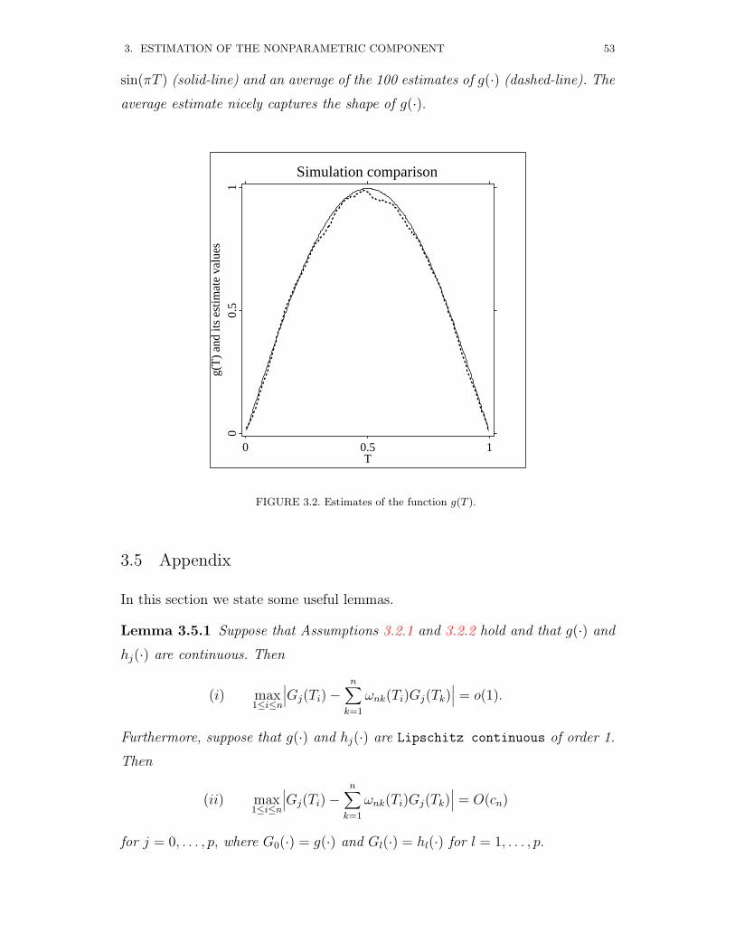
3. ESTIMATION OF THE NONPARAMETRIC COMPONENT 53
sin(πT ) (solid-line) and an average of the 100 estimates of g(·) (dashed-line). The
average estimate nicely captures the shape of g(·).
Simulation comparison
0 0.5 1T
00.
51
g(T
) an
d its
est
imat
e va
lues
FIGURE 3.2. Estimates of the function g(T ).
3.5 Appendix
In this section we state some useful lemmas.
Lemma 3.5.1 Suppose that Assumptions 3.2.1 and 3.2.2 hold and that g(·) and
hj(·) are continuous. Then
(i) max1≤i≤n
∣∣∣Gj(Ti)−n∑k=1
ωnk(Ti)Gj(Tk)∣∣∣ = o(1).
Furthermore, suppose that g(·) and hj(·) are Lipschitz continuous of order 1.
Then
(ii) max1≤i≤n
∣∣∣Gj(Ti)−n∑k=1
ωnk(Ti)Gj(Tk)∣∣∣ = O(cn)
for j = 0, . . . , p, where G0(·) = g(·) and Gl(·) = hl(·) for l = 1, . . . , p.

54 3. ESTIMATION OF THE NONPARAMETRIC COMPONENT
Proof. The proofs are similar to Lemma A.1. We omit the details.
The following Lemma is a slightly modified version of Theorem 9.1.1 of Chow
and Teicher (1988). We therefore do not give its proof.
Lemma 3.5.2 Let ξnk, k = 1, . . . , kn, be independent random variables with mean
zero and finite variance σ2nk. Assume that lim
n→∞
∑kn
k=1σ2nk = 1 and max1≤k≤kn σ
2nk →
0. Then∑knk=1 ξnk →L N(0, 1) if and only if
kn∑k=1
Eξ2nkI(|ξnk| > δ)→ 0 for any δ > 0 as n→∞.
Lemma 3.5.3 Let V1, . . . , Vn be independent random variables with EVi = 0 and
infiEV2i > C > 0 for some constant number C. There exists a function H(v)
satisfying∫∞
0 vH(v)dv <∞ such that
P|Vk| > v ≤ H(v) for large enough v > 0 and k = 1, . . . , n. (3.5.1)
Also assume that ani, i = 1, . . . , n, n ≥ 1 is a sequence of real numbers satisfying∑ni=1 a
2ni = 1. If max1≤i≤n |ani| → 0, then for a′ni = ani/σi(V ),
n∑i=1
a′niVi −→L N(0, 1) as n→∞.
where σi(V ) is the variance of Vi.
Proof. Denote ξnk = a′nkVk, k = 1, . . . , n. We have∑nk=1 Eξ
2nk = 1. Moreover, it
follows that
n∑k=1
Eξ2nkI(|ξnk| > δ) =
n∑k=1
a′nk2EV 2
k I(|ankVk| > δ)
=n∑k=1
a2nk
σ2k
EV 2k I(|ankVk| > δ)
≤ (infkσ2k)−1 sup
kEV 2
k I(|ankVk| > δ).
It follows from the condition (3.5.1) that
supkEV 2
k I(|ankVk| > δ) → 0 as n→∞.
Therefore Lemma 3.5.3 follows from Lemma 3.5.2.

4ESTIMATION WITH MEASUREMENTERRORS
4.1 Linear Variables with Measurement Errors
4.1.1 Introduction and Motivation
In this section, we are interested in the estimation of the unknown parameter
β and the unknown function g(·) in model (1.1.1) when the covariates Xi are
measured with errors. Instead of observing Xi, we observe
Wi = Xi + Ui, (4.1.1)
where the measurement errors Ui are i.i.d., independent of (Yi, Xi, Ti), with
mean zero and covariance matrix Σuu. We will assume that Σuu is known, taking
up the case that it is estimated in subsection 4.1.4. The measurement error lit-
erature has been surveyed by Fuller (1987) and Carroll, Ruppert and Stefanski
(1995).
It is well known that in linear regression, by applying the so–called correction
for attenuation, inconsistency caused by measurement error can be overcome.
In our context, this suggests that we use the estimator
βn = (WTW − nΣuu)−1WT Y. (4.1.2)
The estimator (4.1.2) can be derived in much the same way as the Severini–
Staniswalis estimator. For every β, let g(T, β) maximize the weighted likelihood
ignoring measurement error, and then form an estimator of β via a negatively
penalized operation:
minimizen∑i=1
Yi −W T
i β − g(Ti, β)2− βTΣuuβ. (4.1.3)
The fact that g(t) = E(Yi −W Ti β|T = t) suggests
gnw(t) =n∑j=1
ωnj(t)(Yj −W Tj βn) (4.1.4)
as the estimator of g(t).

56 4. ESTIMATION WITH MEASUREMENT ERRORS
In some cases, it may be reasonable to assume that the model errors εi are
homoscedastic with common variance σ2. In this event, since EYi − XTi β −
g(Ti)2 = σ2 and EYi −W Ti β − g(Ti)2 = EYi −XT
i β − g(Ti)2 + βTΣuuβ, we
define
σ2n = n−1
n∑i=1
(Yi − W Ti βn)2 − βTnΣuuβn (4.1.5)
as the estimator of σ2. The negative sign in the second term in (4.1.3) looks odd
until one remembers that the effect of measurement error is attenuation, i.e., to
underestimate β in absolute value when it is scalar, and thus one must correct
for attenuation by making β larger, not by shrinking it further towards zero.
In this chapter, we analyze the estimate (4.1.2) and show that it is consistent,
asymptotically normally distributed with a variance different from (2.1.1). Just
as in the Severini–Staniswalis algorithm, a kernel weighting ordinary bandwidth
of order h ∼ n−1/5 may be used.
Subsection 4.1.2 is the statement of the main results for β, while the results
for g(·) are stated in Subsection 4.1.3. Subsection 4.1.4 states the corresponding
results for the measurement error variance Σuu estimated. Subsection 4.1.5 gives
a numerical illustration. Several remarks are given in Subsection 4.1.6. All proofs
are delayed until the last subsection.
4.1.2 Asymptotic Normality for the Parameters
Our two main results are concerned with the limit distributions of the estimates
of β and σ2.
Theorem 4.1.1 Suppose that Assumptions 1.3.1-1.3.3 hold and that E(ε4 +
‖U‖4) <∞. Then βn is an asymptotically normal estimator, i.e.
n1/2(βn − β) −→L N(0,Σ−1ΓΣ−1),
where Γ = E[(ε − UTβ)X − E(X|T )]⊗2 + E(UUT − Σuu)β⊗2 + E(UUT ε2).
Note that Γ = E(ε−UTβ)2Σ+E(UUT−Σuu)β⊗2+Σuuσ2 if ε is homoscedastic
and independent of (X,T ).
Theorem 4.1.2 Suppose that the conditions of Theorem 4.1.1 hold. In addition,
we assume that the ε’s are homoscedastic with variance σ2, and independent of

4. ESTIMATION WITH MEASUREMENT ERRORS 57
(X,T ). Then
n1/2(σ2n − σ2) −→L N(0, σ2
∗),
where σ2∗ = E(ε− UTβ)2 − (βTΣuuβ + σ2)2.
Remarks
• As described in the introduction, an important aspect of the results of
Severini and Staniswalis is that their methods lead to asymptotically normal
parameter estimates in kernel regression, even with the bandwidth of the
usual order hn ≈ n−1/5. The same holds for our estimators in general. For
example, suppose that the design points Ti satisfy that there exist constants
M1 and M2 such that
M1/n ≤ mini≤n|Ti − Ti−1| ≤ max
i≤n|Ti − Ti−1| ≤M2/n.
Then Assumptions 1.3.3(i)-(iii) are satisfied by a simple verification.
• It is relatively easy to estimate the covariance matrix of βn. Let dim(X) be
the number of the components of X. A consistent estimate of Σ is just
n− dim(X)−1n∑i=1
Wi − gw,h(Ti)⊗2 − Σuu(def= Σn).
In the general case, one can use (4.1.15) to construct a consistent sandwich-
-type estimate of Γ, namely
n−1n∑i=1
Wi(Yi − W T
i βn) + Σuuβn⊗2
.
In the homoscedastic case, namely that ε is independent of (X,T, U) with
variance σ2, and with U being normally distributed, a different formula can
be used. Let C(β) = E(UUT −Σuu)β⊗2. Then a consistent estimate of Γ
is
(σ2n + βTnΣuuβn)Σn + σ2
nΣuu + C(βn).
• In the classical functional model, instead of obtaining an estimate of Σuu
through replication, it is instead assumed that the ratio of Σuu to σ2 is
known. Without loss of generality, we set this ratio equal to the identity

58 4. ESTIMATION WITH MEASUREMENT ERRORS
matrix. The resulting analogue of the parametric estimators to the partially
linear model is to solve the following minimization problem:
n∑i=1
∣∣∣∣∣∣ Yi − WTi β√
1 + ‖β‖2
∣∣∣∣∣∣2
= min!,
where ‖ · ‖ denotes the Euclidean norm. One can use the techniques of
this section to show that this estimator is consistent and asymptotically
normally distributed. The asymptotic variance of the estimate of β for the
case where ε is independent of (X,T ) can be shown to be
Σ−1
[(1 + ‖β‖2)2σ2Σ +
E(ε− UTβ)2Γ1ΓT1 1 + ‖β‖2
]Σ−1,
where Γ1 = (1 + ‖β‖2)U + (ε− UTβ)β.
4.1.3 Asymptotic Results for the Nonparametric Part
Theorem 4.1.3 Suppose that Assumptions 1.3.1-1.3.3 hold and that ωni(t) are
Lipschitz continuous of order 1 for all i = 1, . . . , n. If E(ε4 + ‖U‖4) < ∞,
then for fixed Ti, the asymptotic bias and asymptotic variance of gnw(t) are∑ni=1 ωni(t)g(Ti)− g(t) and
∑ni=1 ω
2ni(t)(β
TΣuuβ + σ2), respectively.
If (Xi, Ti) are random, then the bias and variance formulas are the usual ones
for nonparametric kernel regression.
4.1.4 Estimation of Error Variance
Although in some cases, the measurement error covariance matrix Σuu has been
established by independent experiments, in others it is unknown and must be
estimated. The usual method of doing so is by partial replication, so that we
observe Wij = Xi + Uij, j = 1, ...mi.
We consider here only the usual case that mi ≤ 2, and assume that a fraction
δ of the data has such replicates. Let W i be the sample mean of the replicates.
Then a consistent, unbiased method of moments estimate for Σuu is
Σuu =
∑ni=1
∑mij=1(Wij −W i)
⊗2∑ni=1(mi − 1)
.
The estimator changes only slightly to accommodate the replicates, becoming
βn =
[n∑i=1
W i − gw,h(Ti)
⊗2− n(1− δ/2)Σuu
]−1
×n∑i=1
W i − gw,h(Ti)
Yi − gy,h(Ti) , (4.1.6)

4. ESTIMATION WITH MEASUREMENT ERRORS 59
where gw,h(·) is the kernel regression of the W i’s on Ti.
Using the techniques in Subsection 4.1.7, one can show that the limit distri-
bution of (4.1.6) is N(0,Σ−1Γ2Σ−1) with
Γ2 = (1− δ)E[(ε− UTβ)X − E(X|T )
]⊗2
+δE[(ε− UT
β)X − E(X|T )]⊗2
+(1− δ)E([UUT − (1− δ/2)Σuuβ]⊗2 + UUT ε2
)+δE
([UUT − (1− δ/2)Σuuβ]⊗2 + UU
Tε2). (4.1.7)
In (4.1.7), U refers to the mean of two U ’s. In the case that ε is independent of
(X,T ), the sum of the first two terms simplifies to σ2 + βT (1− δ/2)ΣuuβΣ.
Standard error estimates can also be derived. A consistent estimate of Σ is
Σn = n− dim(X)−1n∑i=1
W i − gw,h(Ti)
⊗2− (1− δ/2)Σuu.
Estimates of Γ2 are also easily developed. In the case where ε is homoscedastic
and normal error, the sum of first two terms can be estimated by (σ2n + (1 −
δ/2)βTn Σuuβn)Σn. The sum of the last two terms is a deterministic function of
(β, σ2,Σuu), and these estimates can be simply substituted into the formula.
A general sandwich-type estimator is developed as follows.
Ri = W i(Yi − WT
i βn) + Σuuβn/mi +κ
δ(mi − 1)
1
2(Wi1 −Wi2)⊗2 − Σuu
,
where κ = n−1∑ni=1 m
−1i . Then a consistent estimate of Γ2 is the sample covari-
ance matrix of the Ri’s.
4.1.5 Numerical Example
To illustrate the method, we consider data from the Framingham Heart Study.
We considered n = 1615 males with Y being their average blood pressure in a
fixed 2–year period, T being their age and W being the logarithm of the observed
cholesterol level, for which there are two replicates.
We did two analyses. In the first, we used both cholesterol measurements,
so that in the notation of Subsection 4.1.4, δ = 1. In this analysis, there is not
a great deal of measurement error. Thus, in our second analysis, which is given
for illustrative purposes, we used only the first cholesterol measurement, but
fixed the measurement error variance at the value obtained in the first analysis,

60 4. ESTIMATION WITH MEASUREMENT ERRORS
Kernel fit: SBP on patient Age
40 50 60Patient Age
125
130
135
140
Aver
age S
BP
FIGURE 4.1. Estimate of the function g(T ) in the Framingham data ignoring mea-surement error.
in which δ = 0. For nonparametric fitting, we chose the bandwidth using cross-
validation to predict the response. Precisely we computed the squared error using
a geometric sequence of 191 bandwidths ranging in [1, 20]. The optimal band-
width was selected to minimize the square error among these 191 candidates. An
analysis ignoring measurement error found some curvature in T , see Figure 4.1
for the estimate of g(T ).
As mentioned below, we will consider four cases and use XploRe (Hardle,
Klinke and Muller, 1999) to calculate each case. Our results are as follows.
We first consider the case in which the measurement error is estimated, and
both cholesterol values are used to estimate Σuu. The estimator of β, ignoring
measurement error was 9.438, with an estimated standard error 0.187. When
we accounted for measurement error, the estimate increased to β = 12.540, and
the standard error increased to 0.195.
In the second analysis, we fixed the measurement error variance and used
only the first cholesterol value. The estimator of β, ignoring measurement
error, was 10.744, with an estimated standard error 0.492. When we accounted
for measurement error, the estimate increased to β = 13.690, and the standard
error increased to 0.495.

4. ESTIMATION WITH MEASUREMENT ERRORS 61
4.1.6 Discussions
Our results have been phrased as if the X’s were fixed constants. If they are
random variables, the proofs can be simplified and the same results are obtained,
now with ui = Xi − E(Xi|Ti).The nonparametric regression estimator (4.1.4) is based on locally weighted
averages. In the random X context, the same results apply if (4.1.4) is replaced
by a locally linear kernel regression estimator.
If we ignore measurement error, the estimator of β is given by (1.2.2) but
with the unobserved X replaced by the observed W . This differs from the correc-
tion for the attenuation estimator (4.1.2) by a simple factor which is the inverse
of the reliability matrix (Gleser, 1992). In other words, the estimator which ig-
nores measurement error is multiplied by the inverse of the reliability matrix to
produce a consistent estimator of β. This same algorithm is widely employed in
parametric measurement error problems for generalized linear models, where it
is often known as an example of regression calibration (see Carroll, et al., 1995, for
discussion and references). The use of regression calibration in our semiparametric
context thus appears to be promising when (1.1.1) is replaced by a semiparametric
generalized linear model.
We have treated the case in which the parametric part X of the model has
measurement error and the nonparametric part T is measured exactly. An in-
teresting problem is to interchange the roles of X and T , so that the parametric
part is measured exactly and the nonparametric part is measured with error, i.e.,
E(Y |X,T ) = θT + g(X). Fan and Truong (1993) have discussed the case where
the measurement error is normally distributed, and shown that the nonpara-
metric function g(·) can be estimated only at logarithmic rates, but not with rate
n−2/5. The next section will study this problem in detail.
4.1.7 Technical Details
We first point out two facts, which will be used in the proofs.
Lemma 4.1.1 Assume that Assumption 1.3.3 holds and that E(|ε1|4 + ‖U‖4) <
∞. Then
n−1n∑i=1
εi
n∑j=1
ωnj(Ti)εj
= oP (n−1/2),

62 4. ESTIMATION WITH MEASUREMENT ERRORS
n−1n∑i=1
Uis
n∑j=1
ωnj(Ti)Ujm
= oP (n−1/2), (4.1.8)
for 1 ≤ s,m ≤ p.
Its proof can be completed in the same way as Lemma 5.2.3 (5.2.7). We refer the
details to Liang, Hardle and Carroll (1999).
Lemma 4.1.2 Assume that Assumptions 1.3.1-1.3.3 hold and that E(ε4 +‖U‖4)
<∞. Then the following equations
limn→∞
n−1WTW = Σ + Σuu (4.1.9)
limn→∞
n−1WT Y = Σβ (4.1.10)
limn→∞
n−1YT Y = βTΣβ + σ2 (4.1.11)
hold in probability.
Proof. Since Wi = Xi + Ui and Wi = Xi + Ui, we have
(WTW)sm = (XT X)sm + (UT X)sm + (XT U)sm + (UT U)sm. (4.1.12)
It follows from the strong law of large numbers and Lemma A.2 that
n−1n∑j=1
XjsUjm → 0 a.s. (4.1.13)
Observe that
n−1n∑j=1
XjsUjm = n−1[ n∑j=1
XjsUjm −n∑j=1
n∑k=1
ωnk(Tj)Xks
Ujm
−n∑j=1
n∑k=1
ωnk(Tj)UkmXjs
+n∑j=1
n∑k=1
ωnk(Tj)Xks
n∑k=1
ωnk(Tj)Ukm].
Similar to the proof of Lemma A.3, we can prove that supj≤n |∑nk=1 ωnk(Tj)Ukm| =
oP (1), which together with (4.1.13) and Assumptions 1.3.3 (ii) deduce that the
above each term tends to zero. For the same reason, n−1(UT X)sm also converges
to zero.
We now prove
n−1(UT U)sm → σ2sm, (4.1.14)

4. ESTIMATION WITH MEASUREMENT ERRORS 63
where σ2sm is the (s,m)−th element of Σuu. Obviously
n−1(UT U)sm =1
n
[ n∑j=1
UjsUjm −n∑j=1
n∑k=1
ωnk(Tj)UksUjm
−n∑j=1
n∑k=1
ωnk(Tj)UkmUjs
+n∑j=1
n∑k=1
ωnk(Tj)Uks n∑
k=1
ωnk(Tj)Ukm].
Noting that n−1∑nj=1 UjsUjm → σ2
sm, equation (4.1.14) follows from Lemma A.3
and (4.1.8). Combining (4.1.12), (4.1.14) with the arguments for 1/n(UT X)sm →0 and 1/n(XT U)sm → 0, we complete the proof of (4.1.9).
Next we prove (4.1.10). It is easy to see that
∣∣∣ n∑j=1
Xjsgj∣∣∣ ≤
n∑j=1
X2js
n∑j=1
g2j
1/2
≤ cnn1/2
n∑j=1
X2js
1/2
≤ Cncn,
1
n(WT ε)s → 0 and
1
n
n∑j=1
Ujsgj → 0
as n→∞. Thus,
1
n(WT G)s =
1
n
n∑j=1
Xjsgj +1
n
n∑j=1
Ujsgj
=1
n
n∑j=1
Xjs −
n∑k=1
ωnk(Tj)Xks
gj +
1
n
n∑j=1
Ujsgj → 0
as n→∞. Combining the above arguments with (4.1.9), we complete the proof
(4.1.10). The proof of (4.1.11) can be completed by the similar arguments. The
details are omitted.
Proof of Theorem 4.1.1. Denote ∆n = (WTW − nΣuu)/n. By Lemma 4.1.2
and direct calculations,
n1/2(βn − β) = n−1/2∆−1n (WT Y − WTWβ + nΣuuβ)
= n−1/2∆−1n (XT G + XT ε+ UT G + UT ε
−XT Uβ − UT Uβ + nΣuuβ).
By Lemmas A.2, A.3 and 4.1.1, we conclude that
n1/2(βn − β) = n−1/2∆−1n
n∑i=1
(uiεi − uiUT
i β + Uiεi − UiUTi β + Σuuβ
)+ oP (1)
def= n−1/2
n∑i=1
ζin + oP (1). (4.1.15)

64 4. ESTIMATION WITH MEASUREMENT ERRORS
Since
limn→∞
n−1n∑i=1
ui = 0, limn→∞
n−1n∑i=1
uiuTi = Σ (4.1.16)
and E(ε4 + ‖U‖4) < ∞, it follows that the k−th element ζ(k)in of ζin (k =
1, . . . , p) satisfies that for any given ζ > 0,
1
n
n∑i=1
Eζ(k)in
2I(|ζ(k)
in | > ζn1/2) → 0 as n→∞.
This means that Lindeberg’s condition for the central limit theorem holds.
Moreover,
Cov(ζni) = Eui(εi − UT
i β)2uTi
+ E
(UiUTi − Σuu)β
⊗2+ E(UiU
Ti ε
2i )
+uiE(UTi ββ
TUiUTi ) + E(UiU
Ti ββ
TUi)ui,
which and (4.1.16) imply that
limn→∞
n−1n∑i=1
Cov(ζni) = E(ε− UTβ)2Σ + E(U · UT − Σuu)β⊗2 + E(UUT ε2).
Theorem 4.1.1 now follows.
Proof of Theorem 4.1.2. Denote
An = n−1[
YT Y YTWWT Y WTW
], A =
[βTΣβ + σ2 βTΣ
Σβ Σ + Σuu
],
An = n−1[
(ε+ Uβ)T (ε+ Uβ) (ε+ Uβ)T (U + u)(U + u)T (ε+ Uβ) (U + u)T (U + u)
].
According to the definition of σ2n, a direct calculation and Lemma 4.1.1 yield that
n1/2(σ2n − σ2) = n1/2
5∑j=1
Sjn +1
n1/2(ε− Uβ)T (ε− Uβ)
− n1/2(βTnΣuuβn + σ2) + oP (1),
where S1n = (1,−βTn )(An− An)(1,−βTn )T , S2n = (1,−βTn )(An−A)(0, βT − βTn )T ,
S3n = (0, βT − βTn )A(0, βT − βTn )T , S4n = (0, βT − βTn )(An − A)(1,−βT )T and
S5n = −(β − βn)T (β − βn). It follows from Theorem 4.1.1 and Lemma 4.1.2 that
n1/2∑5j=1 Sjn → 0 in probability and
n1/2(σ2n − σ2) = n−1/2
n∑i=1
(εi − UT
i β)2 − (βTΣuuβ + σ2)
+ oP (1).

4. ESTIMATION WITH MEASUREMENT ERRORS 65
Theorem 4.1.2 now follows immediately.
Proof of Theorem 4.1.3. Since βn is a consistent estimator of β, its asymptotic
bias and variance equal the relative ones of∑nj=1 ωnj(t)(Yj − W T
j β), which is
denoted by g∗n(t). By simple calculations,
Eg∗n(t)− g(t) =n∑i=1
ωni(t)g(Ti)− g(t),
Eg∗n(t)− Eg∗n(t)2 =n∑i=1
ω2ni(t)(β
TΣuuβ + σ2).
Theorem 4.1.3 is immediately proved.
4.2 Nonlinear Variables with Measurement Errors
4.2.1 Introduction
The previous section concerns the case where X is measured with error and T is
measured exactly. In this section, we interchange the roles of X and T so that the
parametric part is measured exactly and the nonparametric part is measured with
error, i.e., E(Y |X,T ) = XTβ+ g(T ) and W = T +U , where U is a measurement
error.
The following theorem shows that in the case of a large sample, there is no
cost due to the measurement error of T when the measurement error is ordinary
smooth or super smooth and X and T are independent. That is, the estimator
of β given in (4.2.4), under our assumptions, is equivalent to the estimator given
by (4.2.2) below when we suppose that Ti are known. This phenomenon looks
unsurprising since the related work on the partially linear model suggests that a
rate of at least n−1/4 is generally needed, and since Fan and Truong (1993) proved
that the nonparametric function estimate can reach the rate of OP (n−k/(2k+2α+1))
< o(n−1/4) in the case of ordinary smooth error. In the case of ordinary
smooth error, the proof of the theorem indicates that g(T ) seldomly affects our
estimate β∗n for the case where X and T are independent.
Fan and Truong (1993) have treated the case where β = 0 and T is observed
with measurement error. They proposed a new class of kernel estimators using
deconvolution and found that optimal local and global rates of convergence of
these estimators depend heavily on the tail behavior of the characteristic function
of the error distribution; the smoother, the slower.
66 4. ESTIMATION WITH MEASUREMENT ERRORS
In model (1.1.1), we assume that εi are i.i.d. and that the covariates Ti are
measured with errors, and we can only observe their surrogates Wi, i.e.,
Wi = Ti + Ui, (4.2.1)
where the measurement errors Ui are i.i.d., independent of (Yi, Xi, Ti), with
mean zero and covariance matrix Σuu. We will assume that U has a known distri-
bution, which was proposed by Fan and Truong (1993) to assure that the model
is identifiable. The model (1.1.1) with (4.2.1) can be seen as a mixture of linear
and nonlinear errors-in-variables models.
Recalling the argument for (1.2.2), it can be obtained as follows. Let gy,h(·)and gx,h(·) be the kernel regression estimators of E(Y |T ) and E(X|T ), respec-
tively. Then
βLS =[ n∑i=1
Xi − gx,h(Ti)⊗2]−1
n∑i=1
Xi − gx,h(Ti)Yi − gy,h(Ti). (4.2.2)
Due to the disturbance of measurement error U and the fact that gx,h(Ti)
and gy,h(Ti) are no longer statistics, the least squares form of (4.2.2) must be
modified. In the next subsection, we will redefine an estimator of β. More exactly,
we have to find a new estimator of g(·) and then perform the regression of Y and
X on W . The asymptotic normality of the resulting estimator of β depends on
the smoothness of the error distribution.
4.2.2 Construction of Estimators
As pointed out in the former subsection, our first objective is to estimate the non-
parametric function g(·) when T is observed with error. This can be overcome
by using the ideas of Fan and Truong (1993). By using the deconvolution tech-
nique, one can construct consistent nonparametric estimates of g(·) with some
convergence rate under appropriate assumptions. First, we briefly describe the
deconvolution method, which has been studied by Stefanski and Carroll (1990),
and Fan and Truong (1993). Denote the densities of W and T by fW (·) and fT (·),respectively. As pointed out in the literature, fT (·) can be estimated by
fn(t) =1
nhn
n∑j=1
Kn
(t−Wj
hn
)with
Kn(t) =1
2π
∫R1
exp(−ist) φK(s)
φU(s/hn)ds, (4.2.3)

4. ESTIMATION WITH MEASUREMENT ERRORS 67
where φK(·) is the Fourier transform of K(·), a kernel function and φU(·) is the
characteristic function of the error variable U . For a detailed discussion, see Fan
and Truong (1993). Denote
ω∗ni(·) = Kn
( · −Wi
hn
)/∑j
Kn
( · −Wj
hn
)def=
1
nhnKn
( · −Wi
hn
)/fn(·).
Now let us return to our goal. Replacing the gn(t) in Section 1.2 by
g∗n(t) =n∑i=1
ω∗ni(t)(Yi −XTi β),
then the least squares estimator β∗n of β can be explicitly expressed as
β∗n = (XT X)−1(XT Y), (4.2.4)
where Y denotes (Y1, . . . , Yn) with Yi = Yi −∑nj=1 ω
∗nj(Wi)Yj and X denotes
(X1, . . . , Xn) with Xi = Xi −∑nj=1 ω
∗nj(Wi)Xj. The estimator β∗n will be shown
to possess asymptotic normality under appropriate conditions.
4.2.3 Asymptotic Normality
Assumption 4.2.1 (i) The marginal density fT (·) of the unobserved covariate
T is bounded away from 0 on [0, 1], and has a bounded k−th derivative, where
k is a positive integer. (ii) The characteristic function of the error distribution
φU(·) does not vanish. (iii) The distribution of the error U is ordinary smooth
or super smooth.
The definitions of super smooth and ordinary smooth distributions were given
by Fan and Truong (1993). We also state them here for easy reference.
1. Super smooth of order α: If the characteristic function of the error distri-
bution φU(·) satisfies
d0|t|α0 exp(−|t|α/ζ) ≤ |φU(t)| ≤ d1|t|α1 exp(−|t|α/ζ) as t→∞, (4.2.5)
where d0, d1, α and ζ are positive constants, and α0 and α1 are constants.
2. Ordinary smooth of order α: If the characteristic function of the error
distribution φU(·) satisfies
d0|t|−α ≤ |φU(t)| ≤ d1|t|−α as t→∞, (4.2.6)
for positive constants d0, d1 and α.

68 4. ESTIMATION WITH MEASUREMENT ERRORS
For example, standard normal and Cauchy distributions are super smooth with
α = 2 and α = 1 respectively. The gamma distribution of degree p and the
double exponential distribution are ordinary smooth with α = p and α = 2,
respectively. We should note that an error cannot be both ordinary smooth and
super smooth.
Assumption 4.2.2 (i) The regression functions g(·) and hj(·) have continuous
kth derivatives on [0, 1].
(ii) The kernel K(·) is a k−th order kernel function, that is∫ ∞−∞
K(u)du = 1,∫ ∞−∞
ulK(u)du
= 0 l = 1, . . . , k − 1,6= 0 l = k.
Assumption 4.2.2 (i) modifies Assumption 1.3.2 to meet the condition 1 of Fan
and Truong (1993).
Our main result is concerned with the limit distribution of the estimate of β
stated as follows.
Theorem 4.2.1 Suppose that Assumptions 1.3.1, 4.2.1 and 4.2.2 hold and that
E(|ε|3 + ‖U‖3) < ∞. If either of the following conditions holds, then β∗n is an
asymptotically normal estimator, i.e., n1/2(βn − β) −→L N(0, σ2Σ−1).
(i) The error distribution is super smooth. X and T are mutually independent.
φK(t) has a bounded support on |t| ≤ M0. We take the bandwidth hn =
c(log n)−1/α with c > M0(2/ζ)1/α;
(ii) The error distribution is ordinary smooth. We take hn = dn−1/(2k+2α+1)
with d > 0 and 2k > 2α + 1.
tαφU(t)→ c, tα+1φ′U(t) = O(1) as t→∞
for some constant c 6= 0,∫ ∞−∞|t|α+1φK(t) + φ′K(t)dt <∞,
∫ ∞−∞|tα+1φK(t)|2dt <∞.
4.2.4 Simulation Investigations
We conduct a moderate sample Monte-Carlo simulation to show the behavior
of the estimator β∗n. A generalization of the model studied by Fan and Truong
(1993) is considered.
Y = XTβ + g(T ) + ε and W = T + U with β = 0.75,

4. ESTIMATION WITH MEASUREMENT ERRORS 69
where X ∼ N(0, 1), T ∼ N(0.5, 0.252), ε ∼ N(0, 0.00152) and g(t) = t3+(1− t)3+.
Two kinds of error distributions are examined to study the effect of them on the
mean squared error (MSE) of the estimator β∗n: one is normal and the other is
double exponential.
1. (Double exponential error). U has a double exponential distribution:
fU(u) = (√
2σ0)−1 exp(−√
2|u|/σ0) for σ20 = (3/7)Var(T ).
Let K(·) be the Gaussian kernel
K(x) = (√
2π)−1 exp(−x2/2),
then
Kn(x) = (√
2π)−1 exp(−x2/2)
1− σ20
2h2n
(x2 − 1). (4.2.7)
2. (Normal error). U ∼ N(0, 0.1252). Suppose the function K(·) has a Fourier
transform by φK(t) = (1− t2)2+. By (4.2.3),
Kn(t) =1
π
∫ 1
0cos(st)(1− s2)3 exp
(0.1252s2
2h2n
)ds. (4.2.8)
For the above model, we use three different kernels: (4.2.7), (4.2.8) and
quartic kernel (15/16)(1−u2)2I(|u| ≤ 1) (ignoring measurement error). Our
aim is to compare the results in the cases of considering measurement error and
ignoring measurement error. The results for different sample numbers are pre-
sented in N = 2000 replications. The mean square errors (MSE) are calculated
based on 100, 500, 1000 and 2000 observations with three kinds of kernels. Table
4.1 gives the final detailed simulation results. The simulations reported show that
the behavior of MSE with double exponential error model is the best one, while
the behavior of MSE with quartic kernel is the worst one.
In the simulation procedure, we also fit the nonparametric part using
g∗n(t) =n∑i=1
ω∗ni(t)(Yi −XTi β∗n), (4.2.9)
where β∗n is the resulting estimator given in (4.2.4).
An analysis ignoring measurement error (with quartic kernel) finds some
curvature in T . See Figure 4.2 for the comparison of g(T ) with its estimator

70 4. ESTIMATION WITH MEASUREMENT ERRORS
TABLE 4.1. MSE(×10−3) of the estimator β∗n
Kernel n = 100 n = 500 n = 1000 n = 2000MSE MSE MSE MSE
(4.2.7) 3.095000 0.578765 0.280809 0.151008(4.2.8) 7.950000 1.486650 0.721303 0.387888quartic 15.52743 10.36125 8.274210 4.166037
(4.2.9) using the different-size samples. Each curve represents the mean of 2000
realizations of these true curves and estimating curves. The solid lines stand for
true values and the dashed lines stand for the values of the resulting estimator
given by (4.2.9).
The bandwidth used in our simulation is selected using cross-validation to
predict the response. More precisely, we compute the average squared error using a
geometric sequence of 41 bandwidths ranging in [0.1, 0.5]. The optimal bandwidth
is selected to minimize the average squared error among 41 candidates. The results
reported here support our theoretical procedure, and illustrate that our estimators
for both the parametric and nonparametric parts work very well numerically.
Samplesize 100
-0.5 0 0.5T
05
1015
0 +
0.00
1 *
g(T)
and
its es
timate
valu
es
Samplesize 1000
-0.5 0 0.5 1T
05
1015
0 +
0.00
1 *
g(T)
and
its es
timate
valu
es
Samplesize 500
-0.5 0 0.5T
05
1015
0 +
0.00
1 *
g(T)
and
its es
timate
valu
es
Samplesize 2000
-0.5 0 0.5 1T
05
1015
0 +
0.00
1 *
g(T)
and
its es
timate
valu
es
FIGURE 4.2. Estimates of the function g(T ).
4.2.5 Technical Details
Lemma 4.2.1 provides bounds for hj(Ti)−∑nk=1 ω
∗nk(Wi)hj(Tk) and g(Ti)−
∑nk=1 ω
∗nk
(Wi)g(Tk). The proof is partly based upon the conclusion of Fan and Truong

4. ESTIMATION WITH MEASUREMENT ERRORS 71
(1993).
Lemma 4.2.1 Suppose that Assumptions 1.3.1 and 4.2.2 hold. Then for all 1 ≤l ≤ p and 1 ≤ i, j ≤ p
E(g∗i g∗j h∗ilh∗jl) = O(h4k),
where
g∗i =1
fT (Wi)
n∑k=1
g(Ti)− g(Tk)1
nhnKn
(Wi −Wk
hn
),
h∗il =1
fT (Wi)
n∑k=1
hl(Ti)− hl(Tk)1
nhnKn
(Wi −Wk
hn
).
Proof. Similar to the proof of Lemma 1 of Fan and Truong (1993), we have
E(g∗i g∗j h∗ilh∗jl) =
1
h4n
∫ ∞−∞· · ·
∫ ∞−∞︸ ︷︷ ︸
8
g(u1)− g(u2)g(u3)− g(u4)hl(v1)− hl(v2)
hl(v3) − hl(v4) ×Kn
(u1 − u2
hn
)Kn
(u3 − u4
hn
)Kn
(v1 − v2
hn
)Kn
(v3 − v4
hn
)fT (u2)fT (u4)fT (v2)fT (v4)
4∏q=1
duq dvq
= O(h4kn )
by applying Assumption 4.2.2.
Proof of Theorem 4.2.1. We first outline the proof of the theorem. We decom-
pose√n(βn−β) into three terms. Then we calculate the tail probability value of
each term. By the definition of β∗n,
√n(β∗n − β) =
√n(XT X)−1
[ n∑i=1
Xigi −n∑i=1
Xi
n∑j=1
ω∗nj(Wi)εj
+n∑i=1
Xiεi]
def= A(n)
[ 1√n
n∑i=1
Xigi −1√n
n∑i=1
Xi
n∑j=1
ω∗nj(Wi)εj
+1√n
n∑i=1
Xiεi], (4.2.10)
where A(n) = n−1XT X and gi = g(Ti) −∑nk=1 ω
∗nk(Wi)g(Tk). Similar to Lemma
A.2 below, we can show that A(n) converges to Σ−1 in probability.
In view of (4.2.10), in order to prove Theorem 4.2.1, it suffices to show thatn∑k=1
Xigi = oP (√n), (4.2.11)
n∑i=1
Xi
n∑j=1
ω∗nj(Wi)εj
= oP (√n), (4.2.12)

72 4. ESTIMATION WITH MEASUREMENT ERRORS
and
1√n
n∑i=1
Xiεi −→L N(0, σ2Σ). (4.2.13)
Obviously for all 1 ≤ j ≤ p
n∑i=1
Xij gi =n∑i=1
uij gi +n∑i=1
hnj(Ti)gi −n∑i=1
n∑q=1
ω∗nq(Wi)uqj gi, (4.2.14)
where hnj(Ti) = hj(Ti)−∑nk=1 ω
∗nk(Wi)hj(Tk).
Similar to the proof of Lemma A.3, we can prove that for 1 ≤ j ≤ p,
max1≤i≤n
∣∣∣ n∑k=1
ω∗nk(Wi)εk∣∣∣ = oP (n−1/4) (4.2.15)
max1≤i≤n
∣∣∣ n∑k=1
ω∗nk(Wi)ukj∣∣∣ = oP (n−1/4). (4.2.16)
Equations (4.2.15) and (4.2.16) will be used repeatedly in the following proof.
Taking r = 3, Vk = ukl of ukj, aji = ω∗ni(Wi), p1 = 2/3, and p2 = 0 in Lemma A.3
below, we can prove both (4.2.15) and (4.2.16).
For the case where U is ordinary smooth error. Analogous to the proof of
Lemma A.3, we can prove that
n∑i=1
uij gi = oP (n1/2). (4.2.17)
Similarly,
∣∣∣ n∑i=1
n∑q=1
ω∗nq(Wi)uqjgi∣∣∣ ≤ nmax
i≤n|gi|max
i≤n
∣∣∣ n∑q=1
ω∗nq(Wi)uqj∣∣∣ = oP (n1/2). (4.2.18)
In view of (4.2.14), (4.2.17) and (4.2.18), in order to prove (4.2.11), it suffices to
show
n∑i=1
hnj(Ti)gi = oP (n1/2)
which is equivalent to
n∑k=1
n∑l=1
n∑i=1
g(Ti)− g(Tk)hj(Ti)− hj(Tl)ωnk(Ti)ωnl(Ti) = oP (n1/2). (4.2.19)
In order to prove (4.2.19), noting that
supt|fn(t)− fT (t)| = oP (1)

4. ESTIMATION WITH MEASUREMENT ERRORS 73
which is similar to Lemma 2 of Fan and Truong (1993), it suffices to shown∑i=1
n∑k=1
n∑l=1
g(Ti)− g(Tk)hj(Ti)− hj(Tl)1
f 2T (Wi)
1
n2h2n
Kn
(Wi −Wk
hn
)Kn
(Wi −Wl
hn
)=
n∑i=1
g∗i h∗ij = oP (
√n),
which follows from for any given δ > 0
P(∣∣∣ n∑i=1
g∗i h∗ij
∣∣∣ > δ√n)≤ 1
nδ2E( n∑i=1
g∗i h∗ij
)2
=1
nδ2
n∑i=1
E(g∗i h∗ij)
2 +n∑i=1
n∑k=1,k 6=i
E(g∗i g∗kh∗ijh∗kj)
=1
nδ2O(nh4k
n ) +O(n2h4kn ) = o(1). (4.2.20)
The last step uses Lemma 4.2.1 and the fact that hn = dn−1/(2k+2α+1) with d > 0
and 2k > 2α + 1.
Thus, equations (4.2.17), (4.2.18) and (4.2.20) imply (4.2.11).
Observe thatn∑i=1
n∑k=1
Xkjω∗ni(Wk)
εi =
n∑i=1
n∑k=1
ukjω∗ni(Wk)
εi
+n∑i=1
n∑k=1
hnj(Tk)ω∗ni(Wk)
εi
−n∑i=1
[ n∑k=1
n∑q=1
uqjω∗nq(Wk)
ω∗ni(Wk)
]εi.(4.2.21)
In order to prove (4.2.12), it suffices to shown∑i=1
n∑k=1
ukjω∗ni(Wk)
εi = op(n
1/2) (4.2.22)
n∑i=1
n∑k=1
hnk(Tj)ω∗ni(Wk)
εi = op(n
1/2) (4.2.23)
n∑i=1
[ n∑k=1
n∑q=1
uqjω∗nq(Wk)
ω∗ni(Wk)
]εi = op(n
1/2) (4.2.24)
Applying (4.2.15) and (4.2.16), equation (4.2.24) follows from∣∣∣ n∑i=1
n∑k=1
n∑q=1
uqjω∗nq(Wk)
ω∗ni(Wk)
εi∣∣∣ ≤ nmaxk≤n
∣∣∣ n∑i=1
ω∗ni(Wk)εi∣∣∣
×maxk≤n
∣∣∣ k∑q=1
uqjω∗nq(Wj)
∣∣∣= op(n
1/2).

74 4. ESTIMATION WITH MEASUREMENT ERRORS
Similar to the proof of Lemma A.3 below, we finish the proof of (4.2.22).
Analogous to (4.2.19)-(4.2.20), in order to prove (4.2.23), it suffices to show
that
1
nhn
n∑i=1
n∑k=1
1
fT (Wi)Kn
(Wk −Wi
hn
)h∗kjεi = oP (n1/2),
which follows from
1
n2h2n
n∑i=1
E n∑k=1
1
fT (Wi)Kn
(Wk −Wi
hn
)h∗kj2Eε2
i = o(n).
Thus, the proof of (4.2.12) follows from (4.2.22)-(4.2.24.)
The proof of (4.2.13) follows from CLT and the fact that 1/nXT X→ Σ holds
in probability as n→∞.
When U is a super smooth error. By checking the above proofs, we find that
the proof of (4.2.11) is required to be modified due to the fact that both (4.2.17)
and (4.2.20) are no longer true when U is a super smooth error.
Similar to (4.2.19)-(4.2.20), in order to prove (4.2.11), it suffices to show that
1
n2h2n
n∑i=1
n∑k=1
(Xij −Xkj)1
fT (Wi)Kn
(Wi −Wk
hn
) n∑k=1
g(Ti)− g(Tk)1
fT (Wi)Kn
(Wi −Wk
hn
)= oP (
√n).
Let
X∗ij =1
nhn
n∑k=1
(Xij −Xkj)1
fT (Wi)Kn
(Wi −Wk
hn
)g∗i =
1
nhn
n∑k=1
g(Ti)− g(Tk)1
fT (Wi)Kn
(Wi −Wk
hn
).
Observe that
E( n∑i=1
X∗ij g∗i
)2=
n∑i=1
E(X∗ij g∗i )
2 +n∑i=1
n∑k=1,k 6=i
E(X∗ij g∗i X∗kj g∗k).
Since Xi and (Ti,Wi) are independent, we have for j = 1, T = (T1, · · · , Tn) and
W = (W1, · · · ,Wn),
E(X∗i1X∗k1|T,W) = E(X11 −X21)(X31 −X21) 1
n2h2n
∑l=1,l 6=i,k

4. ESTIMATION WITH MEASUREMENT ERRORS 75
Kn
(Wi −Wl
hn
)Kn
(Wk −Wl
hn
)+E(X11 −X21)2 1
n2h2n
Kn
(Wi −Wk
hn
)Kn
(Wk −Wi
hn
)+E(X11 −X21)(X31 −X11) 1
n2h2n
∑l=1,l 6=i,k
Kn
(Wi −Wl
hn
)Kn
(Wk −Wi
hn
)
+E(X11 −X21)(X21 −X31) 1
n2h2n
∑l=1,l 6=i,k
Kn
(Wi −Wk
hn
)Kn
(Wk −Wl
hn
)
for all 1 ≤ i, k ≤ n.
Similar to the proof of Lemma 4.2.1, we can show that for all 1 ≤ j ≤ p
E( n∑i=1
X∗ij g∗i
)2= O(nhn).
Finally, for any given η > 0
P∣∣∣ n∑i=1
X∗ij g∗i
∣∣∣ > √nη ≤ 1
nη2E( n∑i=1
X∗ij g∗i
)2= O(hn)→ 0
as n → ∞, which implies (4.2.23) and therefore the proof of Theorem 4.2.1 is
completed.

76 4. ESTIMATION WITH MEASUREMENT ERRORS

5SOME RELATED THEORETIC TOPICS
5.1 The Laws of the Iterated Logarithm
5.1.1 Introduction
The CLT states that the estimator given in (1.2.2) converges to normal distribu-
tion, but does not provide information about the fluctuations of this estimator
about the true value. The laws of iterative logarithm (LIL) complement
the CLT by describing the precise extremes of the fluctuations of the estimator
(1.2.2). This forms the key of this section. The following studies assert that the
extreme fluctuations of the estimators (1.2.2) and (1.2.4) are essentially the same
order of magnitude (2 log log n)1/2 as classical LIL for the i.i.d. case.
The aim of this section is concerned with the case where εi are i.i.d. and
(Xi, Ti) are fixed design points. Similar results for the random design case
can be found in Hong and Cheng (1992a) and Gao (1995a, b). The version of the
LIL for the estimators is stated as follows:
Theorem 5.1.1 Suppose that Assumptions 1.3.1-1.3.3 hold. If E|ε1|3 <∞, then
lim supn→∞
(n
2 log log n
)1/2
|βLSj − βj| = (σ2σjj)1/2, a.s. (5.1.1)
Furthermore, let bn = Cn−3/4(log n)−1 in Assumption 1.3.3 and if Eε41 <∞, then
lim supn→∞
(n
2 log log n
)1/2
|σ2n − σ2| = (V arε2
1)1/2, a.s. (5.1.2)
where βLSj, βj and σjj denote the j−th element of βLS, β and the (j, j)−th
element of Σ−1 respectively.
We outline the proof of the theorem. First we decompose√n(βLS − β) and
√n(σ2
n − σ2) into three terms and five terms respectively. Then we calculate the
tail probability value of each term. We have, from the definitions of βLS and
σ2n, that
√n(βLS − β) =
√n(XT X)−1
n∑i=1
Xigi −n∑i=1
Xi
n∑j=1
ωnj(Ti)εj +n∑i=1
Xiεi
def= n(XT X)−1(H1 −H2 +H3); (5.1.3)
78 5. SOME RELATED THEORETIC TOPICS
√n(σ2
n − σ2) =1√n
YTF − X(XT X)−1XTY −√nσ2
=1√nεT ε−
√nσ2 − 1√
nεT X(XT X)−1XT ε
+1√n
GTF − X(XT X)−1XTG
− 2√n
GT X(XT X)−1XT ε+2√n
GT ε
def=√n(I1 − σ2)− I2 + I3 − 2I4 + 2I5, (5.1.4)
where G = g(T1)− gn(T1), . . . , g(Tn)− gn(Tn)T and gn(·) is given by (1.2.3).
In the following steps we prove that each element of H1 and H2 converges
almost surely to zero, and√nIi also converge almost surely to zero for i =
2, 3, 4, 5. The proof of the first half assertion will be finished in steps 1 and 2. The
proof of the second half assertion will be arranged in Subsection 5.1.3 after we
complete the proof of (5.1.1). Finally, we apply Corollary 5.2.3 of Stout (1974) to
complete the proof of the theorem.
5.1.2 Preliminary Processes
Step 1.
√nH1j =
√n
n∑i=1
xij gi = O(n1/2 log−1/2 n) for j = 1, . . . , p. (5.1.5)
Proof. Recalling the definition of hnij given on the page 29,√nH1j can be de-
composed inton∑i=1
uij gi +n∑i=1
hnij gi −n∑i=1
n∑q=1
ωnq(Ti)uqj gi.
By Lemma A.1, ∣∣∣ n∑i=1
hnij gi∣∣∣ ≤ nmax
i≤n|gi|max
i≤n|hnij| = O(nc2
n).
Applying Abel’s inequality, and using (1.3.1) and Lemma A.1 below, we have for
all 1 ≤ j ≤ p,n∑i=1
uij gi = O(n1/2 log ncn)
and ∣∣∣ n∑i=1
n∑q=1
ωnq(Ti)uqj gi∣∣∣ ≤ nmax
i≤n|gi|max
i≤n
∣∣∣ n∑q=1
ωnq(Ti)uqj∣∣∣
= O(n2/3cn log n).

5. SOME RELATED THEORETIC TOPICS 79
The above arguments imply that
√nH1j = O(n1/2 log−1/2 n) for j = 1, . . . , p.
We complete the proof of (5.1.5).
Step 2.
√nH2j = o(n1/2) for j = 1, . . . , p, a.s. (5.1.6)
Proof. Observe that
√nH2j =
n∑i=1
n∑k=1
xkjωni(Tk)εi
=n∑i=1
n∑k=1
ukjωni(Tk)εi +
n∑i=1
n∑k=1
hnkjωni(Tk)εi
−n∑i=1
[ n∑k=1
n∑q=1
uqjωnq(Tk)ωni(Tk)
]εi.
We now handle these three terms separately. Applying Lemma A.3 with aji =∑nk=1 ukjωni(Tk), r = 2, Vk = εk, 1/4 < p1 < 1/3 and p2 = 1− p1, we obtain that
n∑i=1
n∑k=1
ukjωni(Tk)εi = O(n−(2p1−1)/2 log n), a.s. (5.1.7)
Similarly, by Lemma A.1 and (A.3), we get
∣∣∣ n∑i=1
n∑k=1
hnkjωni(Tk)εi∣∣∣ ≤ nmax
k≤n
∣∣∣ n∑i=1
ωni(Tk)εi∣∣∣maxk≤n|hnkj|
= O(n2/3cn log n), a.s. (5.1.8)
Analogously, applying (A.3) and Abel’s inequality we have
∣∣∣ n∑i=1
[ n∑k=1
n∑q=1
uqjωnq(Tk)ωni(Tk)
]εi∣∣∣ ≤ nmax
k≤n
∣∣∣ n∑i=1
ωni(Tk)εi∣∣∣maxk≤n
∣∣∣ n∑q=1
uqjωnq(Tk)∣∣∣
= O(n1/3 log2 n) = o(n1/2), a.s. (5.1.9)
A combination of (5.1.7)–(5.1.9) yields (5.1.6).
5.1.3 Appendix
In this subsection we complete the proof of the main result. At first, we state a
conclusion, Corollary 5.2.3 of Stout (1974), which will play an elementary role in
our proof.

80 5. SOME RELATED THEORETIC TOPICS
Conclusion S. Let V1, . . . , Vn be independent random variables with mean zero.
There exists a δ0 > 0 such that
max1≤i≤n
E|Vi|2+δ0 <∞ and lim infn→∞
1
n
n∑i=1
V ar(Vi) > 0.
Then
lim supn→∞
|Sn|√2s2
n log log s2n
= 1, a.s.,
where Sn =∑ni=1 Vi and s2
n =∑ni=1 EV
2i .
Recalling that (5.1.3) and (5.1.5) and (5.1.6), in order to complete the proof
of (5.1.1), it suffices to prove
lim supn→∞
|(Σ−1Xε)j|2n log log n
1/2
= (σ2σjj)1/2, a.s. (5.1.10)
By a calculation, we get
1√n
(Σ−1Xε)j =p∑
k=1
σjk[Wk +
1√n
n∑q=1
xqk − hk(Tq)εq]
=p∑
k=1
σjkWk +1√n
n∑q=1
( p∑k=1
σjkuqk)εq,
where
Wk =1√n
n∑i=1
hk(Ti)−
n∑q=1
ωnq(Ti)xqkεi for 1 ≤ k ≤ p.
Analogous to the proof of (A.4), by Lemma A.1 we can prove for all 1 ≤ k ≤ p
|Wk| ≤1√n
∣∣∣ n∑i=1
εihk(Ti)−
n∑q=1
ωnq(Ti)xqk∣∣∣
+1√n
∣∣∣ n∑i=1
n∑q=1
ωnq(Ti)uqk∣∣∣
= O(log n) · o(log−1 n) = o(1) a.s.
using the fact that εi is independent of (Xi, Ti).
Denote Wij =∑pk=1 σ
jkuikεi. Then EWij = 0 for i = 1, . . . , n, and
E|Wij|2+δ0 ≤ C max1≤i≤n
E|εi|2+δ0 <∞,
and
lim infn→∞
1
n
n∑i=1
EW 2ij = σ2(σj1, . . . , σjp)
( 1
nlimn→∞
n∑i=1
uiuTi
)(σj1, . . . , σjp)T
= σ2(σj1, . . . , σjp)Σ(σj1, . . . , σjp)T = σ2σjj > 0.

5. SOME RELATED THEORETIC TOPICS 81
It follows from Conclusion S that (5.1.10) holds. This completes the proof of
(5.1.1).
Next, we prove the second part of Theorem 5.1.1, i.e., (5.1.2). We show that√nIi = o(1) (i = 2, 3, 4, 5) hold with probability one, and then deal with
√n(I1−
σ2).
It follows from Lemma A.1 and (A.3) that
|√nI3| ≤ C
√n max
1≤i≤n
∣∣∣g(Ti)−n∑k=1
ωnk(Ti)g(Tk)∣∣∣2 +
∣∣∣ n∑k=1
ωnk(Ti)εk∣∣∣2
= o(1), a.s.
It follows from Lemma A.1 and (5.1.5) and (5.1.10) that
√nI2 = o(1),
√nI4 = o(1), a.s.
We now consider I5. We decompose I5 into three terms and then prove that each
term is o(n−1/2) with probability one. Precisely,
I5 =1
n
n∑i=1
giεi −n∑k=1
ωni(Tk)ε2k −
n∑i=1
n∑k 6=i
ωni(Tk)εiεk
def= I51 + I52 + I53.
From Lemma A.1, we know that
√nI51 = o(1) and
√nI52 ≤ bnn
−1/2n∑i=1
ε2i = O(log−2 n) = o(1) a.s. (5.1.11)
Observe that
√n|I53| ≤
1√n
∣∣∣ n∑i=1
∑k 6=i
ωnk(Ti)εiεk − In∣∣∣+ In
def=
1√n
(J1n + In),
where In =∑ni=1
∑nj 6=i ωnj(ti)(ε
′j −Eε′j)(ε′i −Eε′i). Similar arguments used in the
proof of Lemma A.3 imply that
J1n ≤ max1≤j≤n
∣∣∣ n∑i=1
ωnj(Ti)εi∣∣∣ n∑i=1
|ε′′i |+ E|εi|′′
+ max1≤j≤n
∣∣∣ n∑i=1
ωnj(Ti)(ε′i − Eε′i)
∣∣∣ n∑i=1
|ε′′i |+ E|ε′′i |
= o(1), a.s. (5.1.12)
It follows from Lemma A.4 and (5.1.12) that
√nI53 = o(1) a.s. (5.1.13)

82 5. SOME RELATED THEORETIC TOPICS
A combination of (5.1.11)–(5.1.13) leads that√nI5 = o(1) a.s.
To this end, using Hartman-Winter theorem, we have
lim supn→∞
(n
2 log log n
)1/2
|I1 − σ2| = (V arε21)1/2 a.s.
This completes the proof of Theorem 5.1.1.
5.2 The Berry-Esseen Bounds
5.2.1 Introduction and Results
It is of theoretical and practical interest to characterize the error of approximation
in the CLT. This section is concerned with establishing the Berry-Esseen bounds
for the estimators defined in (1.2.2) and (1.2.4). Our results focus only on the
case where εi are i.i.d. and (Xi, Ti) are fixed design points. Similar discussions for
the random design case can be found in Hong and Cheng (1992b), Gao (1992),
Gao, Hong and Liang (1995) and Liang (1994b).
In order to state the main results of this section, we need the following addi-
tional assumption.
Assumption 5.2.1
max1≤i≤n
‖ui‖ ≤ B0 <∞, (5.2.1)
lim supn→∞
n1/2|vjk − σjk| <∞ (5.2.2)
for all 1 ≤ j, k ≤ p, where 1/n∑ni=1 uiu
Ti = (vjk)1≤j,k≤p and Σ = (σjk)1≤j,k≤p.
Let βLSj and βj denote the j−th components of βLS and β respectively.
Theorem 5.2.1 Assume that Assumptions 5.2.1 and 1.3.1-1.3.3 hold. Let E|ε1|3
<∞. Then for all 1 ≤ j ≤ p and large enough n
supx
∣∣∣P√n(βLSj − βj)/(σ2σjj)1/2 < x − Φ(x)∣∣∣ = O(n1/2c2
n), (5.2.3)
Furthermore, for cn = Cn−1/2 we have for all 1 ≤ j ≤ p and large enough n
supx
∣∣∣P√n(βLSj − βj)/(σ2σjj)1/2 < x − Φ(x)∣∣∣ = O(n−1/2). (5.2.4)
Theorem 5.2.2 Suppose that Assumptions 5.2.1 and 1.3.1-1.3.3 hold and that
Eε61 <∞. Let bn = Cn−2/3 in Assumption 1.3.3. Then
supx
∣∣∣∣P√n(σ2n − σ2)/
√varε2
1 < x − Φ(x)∣∣∣∣ = O(n−1/2). (5.2.5)

5. SOME RELATED THEORETIC TOPICS 83
Remark 5.2.1 This section mainly establishes the Berry-Esseen bounds for the
LS estimator βLS and the error estimate σ2n. In order to ensure that the two
estimators can achieve the optimal Berry-Esseen bound n−1/2, we assume that the
nonparametric weight functions ωni satisfy Assumption 1.3.3 with cn = cn−1/2.
The restriction of cn is equivalent to selecting hn = cn−1/4 in the kernel regression
case since EβLS−β = O(h4n) +O(h3/2
n n−1/2) under Assumptions 1.3.2 and 1.3.3.
See also Theorem 2 of Speckman (1988). As mentioned above, the n−1/5 rate
for the bandwidth is required for establishing that the LS estimate βLS is√n-
consistent. For this rate of bandwidth, the Berry-Esseen bounds are only of order√nh4
n = n−3/10. In order to establish the optimal Berry-Esseen rate n−1/2, the
faster n−1/4 rate for the bandwidth is required. This is reasonable.
5.2.2 Basic Facts
Lemma 5.2.1 (i) Let Wn = Un + Vn be a sequence of random variables and let
Fn and Gn be the distributions of Wn and Un, respectively. Assume that
‖Gn − Φ‖ ≤ Cn−1/2 and P|Vn| ≥ Cn−1/2 ≤ Cn−1/2.
Then ‖Fn − Φ‖ ≤ Cn−1/2, where ‖Fn − Φ‖ = supx |Fn(x)− Φ(x)|.(ii) Let Wn = AnUn + Bn, where An and Bn are real number sequences such
that |An − 1| < Cn−1/2 and |Bn| < Cn−1/2. Assume that ‖Gn − Φ‖ ≤ Cn−1/2.
Then ‖Fn − Φ‖ ≤ Cn−1/2.
Proof. See Lemma 1 of Zhao (1984).
Lemma 5.2.2 Let V1, · · · , Vn be i.i.d. random variables. Let Zni be the functions
of Vi and Znjk be the symmetric functions of Vj and Vk. Assume that EZni = 0 for
i = 1, · · ·n, and E(Znjk|Vj) = 0 for 1 ≤ j 6= k ≤ n. Furthermore |Cn| ≤ Cn−3/2,
D2n =
1
n
n∑i=1
EZ2ni ≤ C > 0, max
1≤i≤nE|Zni|3 ≤ C <∞,
E|Znjk|2 ≤ d2nj + d2
nk, andn∑k=1
d2nk ≤ Cn.
Putting
Ln =1√nDn
n∑i=1
Zni + Cn∑
1≤i<k≤nZnjk.

84 5. SOME RELATED THEORETIC TOPICS
Then
supx|PLn ≤ x − Φ(x)| ≤ Cn−1/2.
Proof. See Theorem 2 of Zhao (1984).
Lemma 5.2.3 Assume that Assumption 1.3.3 holds. Let Eε61 <∞. Then
P
max1≤i≤n
∣∣∣ n∑k=1
ωnk(Ti)εk∣∣∣ > C1n
−1/4 log n≤ Cn−1/2. (5.2.6)
P∣∣∣ n∑i=1
n∑j 6=i
ωnj(Ti)εjεi∣∣∣ > C1(n/ log n)1/2
≤ Cn−1/2. (5.2.7)
P
max1≤k≤n
∣∣∣ n∑i=1
( n∑j=1
ωnk(Tj)ωni(Tj))εi∣∣∣ > C1n
−1/4 log n≤ Cn−1/2. (5.2.8)
P∣∣∣ n∑i=1
n∑j 6=i
( n∑k=1
ωni(Tk)ωnj(Tk))εjεi
∣∣∣ > C1(n/ log n)1/2≤ Cn−1/2.(5.2.9)
Proof. a) Firstly, let ε′j = εjI(|εj |≤n1/4) and ε′′j = εj − εj for j = 1, · · · , n. By
Assumption 1.3.3(ii) and Eε61 <∞,
P
max1≤i≤n
∣∣∣ n∑j=1
ωnj(Ti)(ε′′j − Eε′′j )
∣∣∣ > C1n−1/4
≤ P n∑j=1
bn(|ε′′j |+ E|ε′′j |) > C1n−1/4
≤ Cbnn1/4( n∑j=1
E|ε′′j |)≤ CbnEε
61
≤ Cn−1/2. (5.2.10)
By Bernstein’s inequality and Assumption 1.3.3(i)(ii), we have
P
max1≤i≤n
∣∣∣ n∑j=1
ωnj(Ti)(ε′j − Eε′j)
∣∣∣ > C1n−1/4 log n
≤n∑i=1
P∣∣∣ n∑j=1
ωnj(Ti)(ε′j − Eε′j)
∣∣∣ > C1n−1/4 log n
≤ 2n∑i=1
exp− C1n
−1/2 log2 n
2∑nj=1 ω
2nj(Ti)Eε
21 + 2C1bn log n
≤ 2n exp−C2
1C log n ≤ Cn−1/2 (5.2.11)
for large enough C1. Combining (5.2.10) with (5.2.11), we finish the proof of
(5.2.6).

5. SOME RELATED THEORETIC TOPICS 85
b) Secondly, let
In =n∑i=1
n∑j 6=i
ωnj(Ti)(ε′j − Eε′j)(ε′i − Eε′i).
Note that
∣∣∣ n∑i=1
n∑j 6=i
ωni(Ti)εiεj − In∣∣∣ ≤ max
1≤i≤n
∣∣∣ n∑j=1
ωnj(Ti)εj∣∣∣ · n∑
j=1
(|ε′′j |+ E|ε′′j |)
+ max1≤j≤n
∣∣∣ n∑i=1
ωnj(Ti)(ε′i − Eε′i)
∣∣∣ · n∑j=1
(|ε′′j |+ E|ε′′j |)
def= Jn. (5.2.12)
By the same reason as (5.2.11),
P
max1≤j≤n
∣∣∣ n∑i=1
ωnj(Ti)(ε′i − Eε′i)
∣∣∣ > C1n−1/4 log n
≤ Cn−1/2. (5.2.13)
Next, by Eε61 <∞ we have
P n∑i=1
(|ε′′i |+ E|ε′′i |) > C1n3/4(log n)−3/2
≤ Cn−3/4(log n)3/2
n∑i=1
E|ε′′i |
≤ Cn1/4(log n)3/2E|ε1|I(|ε1|≥n1/4)
≤ C · n−1/2. (5.2.14)
Thus, by (5.2.6) and (5.2.14) we get
PJn ≥ C1(n/log n)1/2 ≤ Cn−1/2. (5.2.15)
On the other hand, by the similar way as for (5.2.11)
max1≤i≤n
∣∣∣ n∑j=1
ωnj(Ti)(ε′j − Eε′j)
∣∣∣ = O(n−1/4(log n)−1/2) a.s. (5.2.16)
In view of (5.2.12)-(5.2.15), in order to prove (5.2.7), it suffices to show that for
some suitable C1
P|In| > C1(n/log n)1/2 < Cn−1/2 (5.2.17)
whose proof is similar to that of Lemma A.4.
c) The proofs of (5.2.8) and (5.2.9) can be completed by the similar reason
as (5.2.6) and (5.2.7).

86 5. SOME RELATED THEORETIC TOPICS
Lemma 5.2.4 Assume that Assumptions 1.3.1-1.3.3 and that Eε61 < ∞ hold.
Let (a1, · · · , an)j denote the j-th element of (a1, · · · , an). Then for all 1 ≤ j ≤ p
P|(XT ε)j| > cn3/4(log n)−1/4 ≤ Cn−1/2, (5.2.18)
P|(XT G)j| > cn3/4(log n)−1/4 ≤ Cn−1/2. (5.2.19)
Proof. a) Firstly, observe that
(XT ε)j =n∑i=1
uijεi +n∑i=1
hnijεi −n∑i=1
n∑k=1
ωnk(Ti)ukjεi.
Using max1≤i≤n |uij| ≤ C and Assumption 1.3.1, and applying Bernstein’s
inequality for all 1 ≤ j ≤ p,
P∣∣∣ n∑i=1
uij(ε′i − Eε′i)
∣∣∣ > Cn3/4(log n)−1/4
≤ 2 exp
−Cn3/2(log n)−1/2∑n
i=1 u2ijVar(εi) + n1/2(log n)−1/4 max1≤i≤n |uij|
≤ Cn−1/2. (5.2.20)
Similarly by Assumption 1.3.1,
P∣∣∣ n∑i=1
uij(ε′′i − Eε′′i )
∣∣∣ > Cn3/4(log n)−1/4
≤ 2n−3/2(log n)1/2n∑i=1
u2ijE(ε′′i − Eε′′i )2
≤ Cn−2(log n)1/2n∑i=1
u2ijEε
41 ≤ Cn−1/2. (5.2.21)
Thus, by (5.2.20) and (5.2.21) we get
P∣∣∣ n∑i=1
uijεi∣∣∣ > Cn3/4(log n)−1/4
≤ Cn−1/2. (5.2.22)
Analogous to the proof of (5.2.22), using Assumption 1.3.3(i) and max1≤i≤n ‖ui‖ ≤C,
P∣∣∣ n∑i=1
n∑k=1
ωnk(Ti)ukjεi∣∣∣ > Cn3/4(log n)−1/4
≤ Cn−1/2. (5.2.23)
On the other hand, applying Lemma A.3 we have
P∣∣∣ n∑i=1
hnijεi∣∣∣ > Cn3/4(log n)−1/4
≤ Cn−1/2. (5.2.24)

5. SOME RELATED THEORETIC TOPICS 87
Therefore, by (5.2.22)-(5.2.24) we complete the proof of (5.2.18).
b) Secondly, observe that
(XT G)j =n∑i=1
xij −
n∑k=1
ωnk(Ti)xkjg(Ti)− gn(Ti)
=n∑i=1
giuij +n∑i=1
gihnij −n∑k=1
n∑i=1
ωnk(Ti)giukj
−n∑k=1
n∑i=1
ωnk(Ti)hnijεk −
n∑k=1
n∑i=1
ωnk(Ti)uijεk
+n∑k=1
[ n∑i=1
ωnk(Ti) n∑q=1
ωnq(Ti)uqj]εk
def=
6∑k=1
Jkj. (5.2.25)
Applying Abel’s inequality and using Assumption 1.3.1 and Lemma A.1,
Jkj = O(ancn) for k = 1, 3 and J2j = O(nc2n). (5.2.26)
Similar to the proof of (5.2.23), for k = 5, 6
P|Jkj| > Cn3/4(log n)−1/4 ≤ Cn−1/2. (5.2.27)
On the other hand, applying Lemma A.3 we have
P|J4j| > Cn3/4(log n)−1/4 ≤ Cn−1/2. (5.2.28)
Combining (5.2.25)-(5.2.28), we complete the proof of (5.2.19).
5.2.3 Technical Details
The proof of Theorem 5.2.1
Here we prove only the case of j = 1, and the others follow by the same reason.
Denote n−1XT X = (ajk)1≤j,k≤p, n(XT X)−1 = (ajk)1≤j,k≤p,
pni =p∑j=1
a1jxij −
n∑k=1
ωnk(Ti)xkj
=p∑j=1
a1jxij,
qni = pni −n∑k=1
ωnk(Ti)pnk. (5.2.29)
Then, by Assumption 1.3.1 we have
n1/2(βn1 − β1) = n−1/2n∑i=1
qniεi + n1/2n∑i=1
pnigi. (5.2.30)
88 5. SOME RELATED THEORETIC TOPICS
Noting that Assumptions 1.3.1, 1.3.2 and 1.3.3(i) and
max1≤i≤n
|xij| ≤ max1≤i≤n
|hj(Ti)|+ max1≤i≤n
|uij| ≤ C <∞,
we obtain for large enough n
max1≤i≤n
|pni| ≤ C and max1≤i≤n
|qni| ≤ C.
Let Zni = qniεi, then EZni = 0, and
D2n = n−1
n∑i=1
EZ2ni = n−1σ2
n∑i=1
q2ni ≥ C > 0,
max1≤i≤n
E|Zni|3 = max1≤i≤n
|qni|3E|ε1|3 ≤ C <∞.
It follows from (5.2.39) that
D2n = n−1σ2
n∑i=1
q2ni ≥ C > 0 for large enough n
Therefore, by Lemma 5.2.2 we obtain
supx
∣∣∣Pn−1/2D−1n
n∑i=1
Zni < x− Φ(x)
∣∣∣ ≤ Cn−1/2. (5.2.31)
In the following, we need to determine the order of D2n.
Let aj = (aj1, · · · , ajp)T and σj = (σj1, · · · , σjp)T for 1 ≤ j ≤ p. By Lemma
A.2(i) we get
limn→∞
n−1n∑i=1
p2ni = lim
n→∞n−1(a1)T
n∑i=1
xixTi · (a1)
= (σ1)T · Σ · (σ1) = σ11. (5.2.32)
We now prove
n∑i=1
n∑j=1
ωni(Tj)pnj2
= O(n1/2). (5.2.33)
Denote
mks =n∑i=1
ωni(Tk)ωni(Ts), 1 ≤ k 6= s ≤ n, ms =n∑k=1
mkspnk.
By Abel’s inequality, we obtain
∣∣∣ n∑i=1
pnimi
∣∣∣ ≤ 6 max1≤k≤n
∣∣∣ k∑i=1
pni∣∣∣ · max
1≤i≤n|mi|, (5.2.34)
|ms| =∣∣∣ n∑i=1
pnimis
∣∣∣ ≤ 6 max1≤k≤n
∣∣∣ k∑i=1
pni∣∣∣ · max
1≤k,s≤nωnk(Ts) (5.2.35)

5. SOME RELATED THEORETIC TOPICS 89
and
max1≤k≤n
∣∣∣ n∑s=1
k∑i=1
ωns(Ti)usj∣∣∣ = O(an). (5.2.36)
Also, by Assumption 1.3.1 and Lemma A.1, we have
max1≤k≤n
∣∣∣ k∑i=1
pni∣∣∣ ≤ max
1≤k≤n
∣∣∣ p∑j=1
k∑i=1
xija1j∣∣∣ ≤ max
1≤k≤n
∣∣∣ p∑j=1
k∑i=1
uija1j∣∣∣
+ max1≤k≤n
∣∣∣ p∑j=1
[ k∑i=1
n∑s=1
ωns(Ti)hj(Ts)− hj(Ti)]a1j∣∣∣
+ max1≤k≤n
∣∣∣ p∑j=1
k∑i=1
n∑s=1
ωns(Ti)usja1j∣∣∣
= O(an) +O(ncn). (5.2.37)
Thus, by Assumption 1.3.3, (5.2.32) and (5.2.34)-(5.2.37), we obtain
n∑s=1
[ n∑k 6=s
n∑i=1
ωni(Tk)ωni(Ts)pnk
]pns = O(a2
nbn) +O(n2bnc2n)
and
n∑i=1
n∑k=1
ωni(Tk)pnk2
=n∑s=1
n∑k=1
ω2ni(Tk)p
2nk +
n∑i=1
n∑k 6=s
ωni(Tk)ωni(Ts)pnkpns
= O(nbn) +O(a2nbn) +O(n2bnc
2n)
= O(n3/2cn). (5.2.38)
On the other hand, by (5.2.32), (5.2.38) and the definition of qni, we obtain
limn→∞
n−1n∑i=1
q2ni = lim
n→∞n−1
n∑i=1
p2ni = σ11 > 0. (5.2.39)
Furthermore, by (5.2.29) and Lemma A.2(ii) we have for all (j, k)
|ajk − σjk| ≤ Cn−1/2 and∣∣∣n−1
∑i=1
p2ni − σ11
∣∣∣ ≤ Cn−1/2.
Also, by (5.2.35), (5.2.38), and Assumption 1.3.3(ii) and using the similar reason
as (5.2.34),
∣∣∣n−1n∑i=1
q2ni − σ11
∣∣∣ ≤ ∣∣∣n−1n∑i=1
p2ni − σ11
∣∣∣+ n−1n∑i=1
n∑k=1
ωni(Tk)pnk2
+12n−1 max1≤k≤n
∣∣∣ k∑i=1
pni∣∣∣ · max
1≤i≤n
∣∣∣ n∑k=1
ωni(Tk)pnk∣∣∣
≤ Cn1/2c2n. (5.2.40)

90 5. SOME RELATED THEORETIC TOPICS
By the similar reason as in the proof of (5.2.34), using (5.2.37), Lemma A.1, and
Assumption 1.3.3, we obtain
∣∣∣ n∑i=1
pnigi∣∣∣ ≤ 6 max
1≤k≤n
∣∣∣ k∑i=1
pni∣∣∣ max
1≤i≤n|gi| ≤ Cnc2
n. (5.2.41)
Therefore, by (5.2.30), (5.2.31), (5.2.40) and (5.2.41), and using the conditions of
Theorem 5.2.1, we have
supx
∣∣∣P√n(βLS1 − β1)/(σ2σ11)1/2 < x − Φ(x)∣∣∣ = O(n1/2c2
n).
Thus, we complete the proof of (5.2.3). The proof of (5.2.4) follows similarly.
The proof of Theorem 5.2.2
In view of Lemmas 5.2.1 and 5.2.2 and the expression given in (5.1.4), in order
to prove Theorem 5.2.2, we only need to prove P√n|Ik| > Cn−1/2 < Cn−1/2
for k = 2, 3, 4, 5 and large enough C > 0, which are arranged in the following
lemmas.
Lemma 5.2.5 Assume that Assumptions 1.3.1-1.3.3 hold. Let Eε61 <∞. Then
P|√nI2| > Cn−1/2 ≤ Cn−1/2.
Proof. According to the definition of I2, it suffices to show that
P
1√nεTU(UTU)−1UT ε| > C1n
−1/2
≤ C2√
n
for some constants C1 > pEε21 and C2 > 0. Let pij denote the (i, j) element of
the matrix U(UTU)−1UT . We now have
PεTU(UTU)−1UT ε > C1
= P
n∑i=1
piiε2i +
n∑i=1
∑j 6=i
pijεiεj > C1
= P
n∑i=1
pii(ε2i − Eε2
i )
+n∑i=1
∑j 6=i
pijεiεj > C1 − pEε21
≤ P
∣∣∣∣∣n∑i=1
pii(ε2i − Eε2
i )
∣∣∣∣∣ > 1
2(C1 − pEε2
1)
+P
∣∣∣∣∣∣n∑i=1
∑j 6=i
pijεiεj
∣∣∣∣∣∣ > 1
2(C1 − pEε2
1)
def= I21 + I22.

5. SOME RELATED THEORETIC TOPICS 91
Using (5.2.1) we have
I21 ≤1
C22
E
n∑i=1
pii(ε2i − Eε2
i )
2
≤ max1≤i≤n
piip
C22
E(ε2i − Eε2
i )2 ≤ C3
n,
where C2 = 12(C1 − pEε2
1) and C3 > 0 is a constant.
Similarly, we can show that I22 ≤ C/√n.
Lemma 5.2.6 Assume that Assumptions 1.3.1 and 1.3.3 hold. Let Eε61 < ∞.
Then P|√nI3| > Cn−1/2 ≤ Cn−1/2.
Proof. In view of Lemma A.1 and the definition of G, in order to prove Lemma
5.2.6, it suffices to show that
P
n∑i=1
(n∑k=1
Wnk(Ti)εk
)2
> C1
≤ C2√n
for some positive constant C1 and C2. Observe that
n∑i=1
(n∑k=1
Wnk(Ti)εk
)2
=n∑k=1
(n∑i=1
W 2nk(Ti)
)(εk − Eε2
k)
+n∑i=1
n∑k=1
n∑l 6=k
Wnk(Ti)Wnl(Ti)εkεl + Eε21
n∑k=1
n∑i=1
W 2nk(Ti).
Thus we can finish the proof of Lemma 5.2.6 by using the similar reason as the
proofs of Lemmas 5.2.3 and 5.2.5.
Lemma 5.2.7 Assume that Assumptions 1.3.1-1.3.3 hold. Let Eε61 <∞. Then
P|√nI4| > Cn−1/2 ≤ Cn−1/2. (5.2.42)
Proof. The proof is similar to that of Lemma 5.2.5. We omit the details.
We now handle I5. Observe the following decomposition
1
n
n∑i=1
giεi −n∑k=1
ωnk(Tk)ε2k −
n∑i=1
n∑k 6=i
ωni(Tk)εiεk
def= I51 + I52 + I53. (5.2.43)
For q = 1/4, we have
P√n|I51| > Cn−1/2 ≤ P
∣∣∣ n∑i=1
giεiI(|εi|≤nq)
∣∣∣ > C
+ P∣∣∣ n∑i=1
giεiI(|εi|>nq)
∣∣∣ > C
def= R1n +R2n.
It follows from Bernstein inequality and Lemma A.1 that
R1n ≤ 2 exp−Cn1/2−q < Cn−1/2

92 5. SOME RELATED THEORETIC TOPICS
and
R2n ≤ Cn∑i=1
|gi| · E|εiI(|εi|>nq)|
≤ C max1≤i≤n
|gi|n∑i=1
Eε6in−6q < Cn−1/2.
Combining the conclusions for R1n and R2n, we obtain
P√n|I51| > Cn−1/2 < Cn−1/2. (5.2.44)
By Assumptions 1.3.3 (ii) (iii), we have for any constant C > C0Eε21
P√
n|I52| > Cn−1/2
= P∣∣∣ n∑i=1
ωni(Ti)(ε2i − Eε2
i ) +n∑i=1
ωni(Ti)Eε2i
∣∣∣ > C
≤ P∣∣∣ n∑i=1
ωni(Ti)(ε2i − Eε2
i )∣∣∣ > C − C0Eε
21
≤ C1E
n∑i=1
ωni(Ti)(ε2i − Eε2
i )2
≤ C1 max1≤i≤n
ωni(Ti)n∑i=1
ωni(Ti)E(ε2i − Eε2
i )2
< C1n−1/2, (5.2.45)
where C0 satisfies maxn≥1∑ni=1 ωni(Ti) ≤ C0, C1 = (C − C0Eε
21)−2 and C2 is a
positive constant.
Calculate the tail probability of I53.
P√
n|I53| > Cn−1/2≤ P
∣∣∣ n∑i=1
∑k 6=i
ωnk(Ti)εiεk − In∣∣∣ > C
+ P|In| > C
def= J1n + J2n,
where In =∑ni=1
∑nj 6=i ωnj(Ti)(ε
′j − Eε′j)(ε′i − Eε′i) and ε′i = εiI(|εi|≤nq).
By a direct calculation, we have
J1n ≤ P
max1≤j≤n
∣∣∣ n∑i=1
ωnj(Ti)εi∣∣∣( n∑i=1
|ε′′i |+ E|εi|′′) > C
+P
max1≤j≤n
∣∣∣ n∑i=1
ωnj(Ti)(ε′i − Eε′i)
∣∣∣( n∑i=1
|ε′′i |+ E|ε′′i |) > C
def= J1n1 + J1n2.
Similar to the proof of (5.2.11), we have
P
max1≤j≤n
∣∣∣ n∑i=1
ωnj(Ti)(ε′i − Eε′i)
∣∣∣ > Cn−1/4

5. SOME RELATED THEORETIC TOPICS 93
≤ 2n∑j=1
P∣∣∣ n∑i=1
ωnj(Ti)(ε′i − Eε′i)
∣∣∣ > Cn−1/4
≤ 2n∑j=1
exp(− cn−1/2
2∑ni=1 ω
2nj(Ti)Eε
21 + 2Cbn
)≤ 2n exp(−Cn−1/2b−1
n ) ≤ Cn−1/2. (5.2.46)
On the other hand, applying Chebyshev’s inequality,
P n∑i=1
|ε′′i |+ E|ε′′i | > Cn1/4≤ Cn−1/4E
n∑i=1
|ε′′i |
≤ Cn−1/4n∑i=1
Eε6in−5/4 < Cn−1/2. (5.2.47)
Hence, (5.2.46) and (5.2.47) imply
J1n2 < Cn−1/2. (5.2.48)
Similar to (5.2.46) and (5.2.47) we have
J1n1 < Cn−1/2. (5.2.49)
Combining (5.2.48) with (5.2.49), we obtain
J1n < Cn−1/2. (5.2.50)
Thus, from (5.2.50) and Lemma A.4, we get
P√n|I53| > Cn−1/2 < Cn−1/2. (5.2.51)
It follows from (5.2.43), (5.2.44), (5.2.45) and (5.2.51) that
P√n|I5| > Cn−1/2 < Cn−1/2. (5.2.52)
The proof of Theorem 5.2.2. From Lemmas 5.2.5, 5.2.6, 5.2.7 and (5.2.52),
we have
P
√n
Var(ε21)
∣∣∣−I2 + I3 − 2I4 + 2I5
∣∣∣ > Cn−1/2
< Cn−1/2. (5.2.53)
Let Zni = ε2i − σ2 and Znij = 0. Then D2
n = 1/n∑ni=1 EZ
2ni = V ar(ε2
1) and
E|Zni|3 ≤ E|ε21 − σ2|3 <∞, which and Lemma 5.2.2 imply that
supx|P√nD−1
n (I1 − σ2) < x − Φ(x)| < Cn−1/2. (5.2.54)
Applying Lemma 5.2.1, (5.2.53) and (5.2.54), we complete the proof of Theorem
5.2.2.

94 5. SOME RELATED THEORETIC TOPICS
5.3 Asymptotically Efficient Estimation
5.3.1 Motivation
Recently, Cuzick (1992a) constructed asymptotically efficient estimators for
β for the case where the error density is known. The problem was extended later
to the case of unknown error distribution by Cuzick (1992b) and Schick (1993).
Golubev and Hardle (1997), under the assumption that X and T are mutually
independent, investigated the second order risk, and calculated it exactly up
to constant. Their further study shows that the spline estimator (Heckman (1986)
and Rice (1986)) is not a second order minimax estimator.
In this section, we shall consider the case where εi are i.i.d. and (Xi, Ti) are
random design points, and construct asymptotically efficient estimators in the
sense of normality, i.e., their asymptotically variance reaches an optimum value.
Our construction approach is essentially based on the following fact (Cheng,
Chen, Chen and Wu 1985, p256): Let W1, . . . ,Wn be i.i.d. random variables drawn
from the density function s(w, θ). Set
Z(w, θ) =∂
∂θlog s(w, θ) and Bn(θ) =
1
n
n∑i=1
∂Z(Wi, θ)
∂θ
If θn is a nα(α > 1/4)-order consistent estimator of θ, then under appropriate
regularity conditions,
θMn = θn −1
nB−1n (θn)
n∑i=1
Z(Wi, θn)
is an asymptotically efficient estimator of θ. See also Stone (1975) and
Schick (1986).
5.3.2 Construction of Asymptotically Efficient Estimators
The efficiency criterion we shall be using in this section is a least dispersed
regular estimator as elaborated in Begun, Hall, Huang and Wellner (1983). See
Bickel, Klaasen, Ritov and Wellner (1993).
In order to derive asymptotically efficient estimators of β, we assume
that there exist a root-n rate estimator β of β and a n−1/3 log n-nonparametric
estimator g(t) of g(t). See, for example, the estimators given in (1.2.2) and (1.2.3).
We assume that the random error ε has a density function ϕ(·) which has finite

5. SOME RELATED THEORETIC TOPICS 95
Fisher information
I =∫ ϕ′2
ϕ(y) dy <∞.
The covariance of the asymptotically efficient estimator of β is Σ−1I−1.
See Cuzick (1992b) and Golubev and Hardle (1997). The common root-n rate
estimator is asymptotically normal with covariance matrix Σ−1σ2. Liang (1994a)
showed that a root-n asymptotically normal estimator of β is asymptotically
efficient if and only if ε is Gaussian.
In constructing our estimation procedure, we smooth the density function ϕ
to ensure that it is continuously differentiable, and truncate the integration and
use the split-sample technique.
Let L(y) be the likelihood function of ϕ(y), i.e., L(y) = ϕ′/ϕ(y). Let ψr(z, r)
be the density function of the normal distribution N(0, r−2). Take rn = log n and
f(z, r) =∫ψr(z − y, r)ϕ(y) dy. Obviously f(z, r) is continuously differentiable of
all orders and converges to ϕ(z) as r tends to infinity. Let f ′(z, r) denote the first
derivative of f(z, r) on z. L(z, r) = [f ′(z, r)/f(z, r)]r, where [a]r = a if |a| ≤ r,
−r if a ≤ −r and r if a > r. L(z, r) is also smoothed as
Ln(y, rn) =∫ rn
−rnL(z, rn)ψrn(y − z, rn) dz.
Assume that β1, g1(t) are the estimators of β, g(t) based on the first-half
samples (Y1, X1, T1), · · · , (Ykn , Xkn , Tkn), respectively, while β2, g2(t) are the ones
based on the second-half samples (Ykn+1, Xkn+1, Tkn+1), · · · , (Yn, Xn, Tn), respec-
tively, where kn(≤ n/2) is the largest integer part of n/2. For the sake of simplicity
in notation, we denote Λj = Yj −XTj β − g(Tj), Λn1j = Yj −XT
j β1 − g1(Tj), and
Λn2j = Yj −XTj β2 − g2(Tj).
5.3.2.1 When the Error Density Function ϕ Known
We construct an estimator of β as follows:
β∗n =¯β − 1
nΣ−1I−1
kn∑j=1
XjLn(Λn2j, rn) +n∑
j=kn+1
XjLn(Λn1j, rn),
where¯β, β1, β2 are discretized forms of β, β1, β2 respectively.

96 5. SOME RELATED THEORETIC TOPICS
Theorem 5.3.1 Suppose that Σ is a positive definite matrix and that β, β1, β2;
g(t), g1(t) and g2(t) are root-n rate and n−1/3 log n estimators of β and g(t),
respectively. Then as n→∞
√n(β∗n − β) −→L N(0, I−1Σ−1).
5.3.2.2 When the Error Density Function ϕ Unknown
In this case, β∗n is not a statistic any more since L(z, rn) contains the unknown
function ϕ and I is also unknown. We estimate them as follows. Set
fn(z, r) =1
n
kn∑j=1
ψrn(z − Λn2j, r) +n∑
j=kn+1
ψrn(z − Λn1j, r),
f ′n(z, r) =∂fn(z, r)
∂z,
Ln(z, rn) =[f ′n(z, rn)
fn(z, rn)
]rn
, An(rn) =∫ rn
−rnL2n(z, rn)fn(z, rn) dz.
Define
βn =¯β − Σ−1
nAn(rn)
∫ rn
−rnLn(z, rn)
kn∑j=1
Xjψrn(z − Λn2j, rn)
+n∑
j=kn+1
Xjψrn(z − Λn1j, rn)dz
as the estimator of β.
Theorem 5.3.2 Under the condition of Theorem 5.3.1, we have as n→∞
√n(βn − β) −→L N(0, I−1Σ−1).
Remark 5.3.1 Theorems 5.3.1 and 5.3.2 show us that the estimators β∗n and βn
are both asymptotically efficient.
Remark 5.3.2 Generally Σ is unknown and must be estimated. To do so, let
gx,h(·) be the kernel regression estimator of E(X|T ). Then
1
n
n∑i=1
Xi − gx,h(Ti)Xi − gx,h(Ti)T
is a consistent estimator of Σ.

5. SOME RELATED THEORETIC TOPICS 97
5.3.3 Four Lemmas
In the following Lemmas 5.3.1 and 5.3.2, a1 and ν are constants satisfying 0 <
a1 < 1/12 and ν = 0, 1, 2.
Lemma 5.3.1 As n sufficiently large,
|ψ(ν)rn (x, rn)| < Cνr
2+2νn ψrn(x, rn) + ψ1−a1
rn (x, rn)
uniformly on x, where Cν is a positive constant depending only on a1 and ν.
Proof. Let n be large enough such that a1r2n > 1. Then exp(x2a1r
2n/2) > |x|ν if
|x|ν > ra1n , and |x|ν exp(−x2r2
n/2) ≤ exp −(1− a1)x2r2n/2 holds. If |x|ν ≤ ra1
n ,
then |x|ν exp(−x2r2n/2) ≤ ra1
n exp(−x2r2n/2). These arguments deduce that
|x|ν exp(−x2r2n/2) ≤ ra1
n
[exp −(1− a1)x2r2
n/2+ exp(−x2r2n/2)
]holds uniformly on x. The proof of this lemma immediately follows.
Lemma 5.3.2 Let M be a given positive constant. Then
sup|t|≤Mn−1/4
ψrn(x+ t, rn) ≤ 3ψrn(x, rn) + ψ1−a1rn (x, rn)
holds uniformly on x as n sufficiently large.
Proof. Let n be large enough such that
n1/4r4n > 2Ma1 log rn. (5.3.1)
Denote an = r−2n n1/4M−1. |x| < an implies |xr2
nt| < 1, and so∣∣∣∣∣ψrn(x+ t, rn)
ψrn(x, rn)
∣∣∣∣∣ = exp−(2xt+ t2)rn/2 = exp(−xtr2n) ≤ e.
When |x| ≥ an, it follows from (5.3.1) that |x| > 2r2na1 log rn. A direct calculation
implies
ψrn(x+ t, rn)
ψ1−a1rn (x, rn)
< 1 < e.
The proof of the lemma is immediately derived.

98 5. SOME RELATED THEORETIC TOPICS
Lemma 5.3.3
(i) supy|L(ν)
n (y, rn)| = O(rν+1n );
(ii) limn→∞
∫ 1
0
∫Ln(y − vn(t), rn)− Ln(y, rn)2ϕ(y)h(t) dy dt = 0 (5.3.2)
if∫ 1
0v2n(t)h(t) dt = O(n−2/3 log2/3 n).
Proof. By the definition of L(ν)n (y, rn), we obtain
rn
∫ rn
−rn|ψ(ν)rn (y − z, rn)| dz ≤ rn
∫ ∞−∞|ψ(ν)rn (y − z, rn)| dz = O(rν+1
n ).
We complete the proof of (i).
Applying the Taylor expansion, Ln(y−vn(t), rn)−Ln(y, rn) = L′n(yn, rn)vn(t),
where yn is between y and y − vn(t). The left-hand side of (5.3.2) equals
limn→∞
∫ 1
0
∫L′n(yn, rn)vn(t)2ϕ(y)h(t) dy dt,
which is bounded by
limn→∞
∫ 1
0
∫supy|L′n(y, rn)|2v2
n(t)ϕ(y)h(t) dy dt.
The proof of (ii) is derived by (i) and the assumption.
Lemma 5.3.4∫ rn
−rn
f (ν)n (z, rn)− f (ν)(z, rn)2
f(z, rn)dz = Op(n
−2/3 log2 n)r4ν+2a1+6n . (5.3.3)∫ rn
−rnf (ν)
n (z, rn)− f (ν)(z, rn)2 dz = Op(n−2/3 log2 n)r4ν+2a1+5
n . (5.3.4)
Proof. The proofs of (5.3.3) and (5.3.4) are the same. We only prove the first one.
The left-hand side of (5.3.3) is bounded by
2∫ rn
−rn
1
n
kn∑j=1
ψ(ν)rn (z − Λn2j, rn)− f (ν)(z, rn)
f 1/2(z, rn)
2dz
+2∫ rn
−rn
1
n
n∑j=1+kn
ψ(ν)rn (z − Λn1j, rn)− f (ν)(z, rn)
f 1/2(z, rn)
2dz
def= 2(W1n +W2n).
Similarly,
W1n ≤ 2∫ rn
−rn
1
n
kn∑j=1
ψ(ν)rn (z − Λn2j, rn)− ψ(ν)
rn (z − Λj, rn)
f 1/2(z, rn)
2dz
+2∫ rn
−rn
1
n
kn∑j=1
ψ(ν)rn (z − Λj, rn)− f (ν)(z, rn)
f 1/2(z, rn)
2dz
def= (W
(1)1n +W
(2)1n ).

5. SOME RELATED THEORETIC TOPICS 99
By the Taylor expansion,
W(1)1n =
∫ rn
−rn
1
n
kn∑j=1
ψ(ν+1)rn (z − Λj + µnjtn2j, rn)
f 1/2(z, rn)tn2j
2dz,
where tn2j = Λn2j − Λj for j = 1, · · · , kn and µnj ∈ (0, 1). It follows from the
assumptions on β2 and g2(t) that tn2j = Op(n−1/3 log n). It follows from Lemma
5.3.2 that W(1)1n is smaller than
Op(n−2/3 log2 n)r4ν+2a1+5
n ·∫ rn
−rn
1
n
kn∑j=1
ψrn(z − Λj, rn)
f(z, rn)dz. (5.3.5)
Noting that the mean of the latter integrity of (5.3.5) is smaller than 2rn, we
conclude that
W(1)1n = Op(n
−2/3 log2 n)r4ν+2a1+6n . (5.3.6)
Similar to (5.3.5), we have
EW(2)1n =
∫ rn
−rn
kn∑j=1
Eψ(ν)rn (z − Λj, rn)− f (ν)(z, rn)2
n2f(z, rn)dz
≤∫ rn
−rn
kn∑j=1
Eψ(ν)rn (z − Λj, rn)2
n2f(z, rn)dz
≤ Cn−1r4ν+2a1+2n .
Thus, we obtain that W1n = Op(n−2/3 log2 n)r4ν+2a1+6
n .
The same conclusion is true for W2n. We therefore complete the proof of
Lemma 5.3.4.
5.3.4 Appendix
Proof of Theorem 5.3.1. To prove Theorem 5.3.1 is equivalent to checking As-
sumptions A.1-A.3 of Schick (1986). The verifications of A.3.1 and A.3.2 are
obvious. Lemma 5.3.3 can be applied to finish the verifications of Assumptions
A.3.4 and A.3.5 in Schick (1986). We omit the details.
Proof of Theorem 5.3.2. We now provide an outline of the proof of Theorem
5.3.2 as follows. Denote
A(rn) =∫ rn
−rnL2n(y, rn)f(y, rn) dy,
βn =¯β − 1
nA(rn)Σ−1
kn∑j=1
XjLn(Λn2j, rn) +n∑
j=kn+1
XjLn(Λn1j, rn).
100 5. SOME RELATED THEORETIC TOPICS
It is easily shown that A(rn)→ I, which means that βn is also an asymptotically
efficient estimator of β when ϕ is known. If we can show that√n(βn − βn)
converges to zero, then the proof of Theorem 5.3.2 is completed.
Note that
βn − βn =1
An(rn)(S1n + S2n) +
1
An(rn)A(rn)(S3n + S4n),
where
S1n =1
n
kn∑j=1
Xj
∫ rn
−rnLn(z, rn)ψrn(z − Λn2j, rn) dz − Ln(Λj, rn)
,
S2n =1
n
n∑j=kn+1
Xj
∫ rn
−rnLn(z, rn)ψrn(z − Λn1j, rn) dz − Ln(Λj, rn)
,
S3n =1
nAn(rn)− A(rn)
kn∑j=1
XjLn(Λn2j, rn),
S4n =1
nAn(rn)− A(rn)
n∑j=kn+1
XjLn(Λn1j, rn).
To prove Theorem 5.3.2 is equivalent to proving ‖Sln‖ = o(n−1/2) for l = 1, 2, 3, 4.
We shall complete these proofs in three steps. Step 1 shows ‖S1n‖ = o(n−1/2) and
‖S2n‖ = o(n−1/2). Step 2 analyzes the first part of S3n, An(rn)−A(rn), and derives
its convergence rate. Step 3 handles the second part of S3n, and then completes
the proof of ‖S3n‖ = o(n−1/2). The same arguments may be used for proving
‖S4n‖ = o(n−1/2). We omit the details.
STEP 1 ‖S1n‖ = op(n−1/2) and ‖S2n‖ = op(n
−1/2).
Proof. It is easy to see that
S1n =∫ rn
−rnLn(z, rn)− L(z, rn)
1
n
kn∑j=1
Xjψrn(z − Λn2j, rn)dz
=∫ rn
−rnLn(z, rn)− L(z, rn) 1
n
kn∑j=1
Xjψrn(z − Λn2j, rn)− f(z, rn)] dz.
(i) When n2fn(z, rn) ≤ 1, it follows from Lemma 5.3.1 that
‖S1n‖ =∥∥∥∫ rn
−rnLn(z, rn)− L(z, rn) 1
n
kn∑j=1
Xjψrn(z − Λn2j, rn) dz∥∥∥
≤ 2rn
∫ rn
−rn
1
n
kn∑j=1
‖Xj‖ψrn(z − Λn2j, rn) dz
≤ 2rn
∫ rn
−rn
1
n2
kn∑j=1
‖Xj‖ dz
= Op(n−1r2
n).

5. SOME RELATED THEORETIC TOPICS 101
(ii) When n2f(z, rn) ≤ 1, ‖S1n‖ is bounded by
2rn
√√√√√∫ rn
−rn
1
n
kn∑j=1
‖Xj‖2
√√√√√∫ rn
−rn
kn∑j=1
ψ2rn(z − Λn2j, rn) dz.
It follows from Lemmas 5.3.2 and 5.3.1 that
kn∑j=1
ψ2rn(z − Λn2j, rn) = Op(1)
kn∑j=1
ψ2rn(z − Λj, rn) + ψ2−2a1
rn (z − Λj, rn)
= Op(rn)kn∑j=1
ψrn(z − Λj, rn),
and so ‖S1n‖ = Op(r2n)√∫ rn−rn f(z, rn) dz = Op(n
−1r5/2n ).
(iii) When n2f(z, rn) > 1 and n2fn(z, rn) > 1,
‖S1n‖ ≤∫ rn
−rn
∣∣∣∣∣ f ′n(z, rn)
fn(z, rn)− f ′(z, rn)
f(z, rn)
∣∣∣∣∣∥∥∥∥∥ 1
n
kn∑j=1
Xjψrn(z − Λn2j, rn)− f(z, rn)∥∥∥∥∥dz
≤
√√√√√ 1
n
kn∑j=1
‖Xj‖2
∫ rn
−rn
∣∣∣∣∣ f ′n(z, rn)
fn(z, rn)− f ′(z, rn)
f(z, rn)
∣∣∣∣∣×
√√√√√∣∣∣∣∣∣ 1n
kn∑j=1
ψrn(z − Λn2j, rn)− f(z, rn)2
∣∣∣∣∣∣ dz. (5.3.7)
Denote
Q1n =1
n
kn∑j=1
ψrn(z − Λn2j, rn)− f(z, rn)2.
The integration part of (5.3.7) is bounded by
∫ rn
−rn
∣∣∣∣∣ f ′n(z, rn)− f ′(z, rn)
f(z, rn)
∣∣∣∣∣Q1/21n dz
+∫ rn
−rn
∣∣∣∣∣ f ′n(z, rn)
fn(z, rn)
∣∣∣∣∣∣∣∣∣∣ fn(z, rn)− f(z, rn)
f(z, rn)
∣∣∣∣∣Q1/21n dz
≤∫ rn
−rn
|f ′n(z, rn)− f ′(z, rn)|2
f(z, rn)dz∫ rn
−rn
Q1n
f(z, rn)dz
1/2
+r1+a1n n2a1
∫ rn
−rn
|fn(z, rn)− f(z, rn)|2
f(z, rn)
∫ rn
−rn
Q1n
f(z, rn)dz
1/2
.
Similar to (5.3.3), we deduce∫ rn
−rn
Q1n
f(z, rn)dz = Op(n
−2/3 log2 n)r2a1+6n .

102 5. SOME RELATED THEORETIC TOPICS
This fact and Lemma 5.3.4 deduce
‖S1n‖ = op(n−1/2).
A combination of the results in (i), (ii) and (iii) completes the proof of the first
part of Step 1. Similarly we can prove the second part. We omit the details.
STEP 2.
An(rn)− A(rn) = Op(n−2/3+2a1 log2 n)r3a1+4
n . (5.3.8)
Proof. An(rn)− A(rn) can be rewritten as∫ rn
−rnL2n(z, rn)fn(z, rn) dz −
∫ rn
−rnL2(z, rn)f(z, rn) dz
=∫ rn
−rnL2
n(z, rn)− L2(z, rn)fn(z, rn) dz
+∫ rn
−rnL2(z, rn)fn(z, rn)− f(z, rn) dz
def= I1n + I2n.
It follows from Lemma 5.3.4 that I2n = Op(n−2/3 log2 n)ra1+5
n . We next consider
I1n.
(i) When n2fn(z, rn) < 1, |I1n| ≤ 2r2n
∫ rn−rn fn(z, rn) dz = O(n−2r3
n).
(ii) When n2f(z, rn) < 1, it follows from Lemma 5.3.4 that
|I1n| ≤ 2r2n
√∫ rn
−rn|fn(z, rn)− f(z, rn)|2 dzr1/2
n +∫ rn
−rnf(z, rn) dz
= Op(n
−1/3 log n)ra1+5n .
(iii) When n2fn(z, rn) ≥ 1 and n2f(z, rn) ≥ 1,
|I1n| ≤∫ rn
−rn|Ln(z, rn)− L(z, rn)||Ln(z, rn) + L(z, rn)|fn(z, rn) dz
≤ 2rn
∫ rn
−rn
∣∣∣∣∣ f ′n(z, rn)
fn(z, rn)− f ′(z, rn)
f(z, rn)
∣∣∣∣∣ fn(z, rn) dz
≤ 2rn
[∫ rn
−rn|f ′n(z, rn)− f ′(z, rn)| dz
+∫ rn
−rn
∣∣∣∣∣f ′(z, rn)
f(z, rn)
∣∣∣∣∣ |fn(z, rn)− f(z, rn)| dz].
It follows from Lemma 5.3.4 and Cauchy-Schwarz inequality that
I1n = Op(n−1/3 log n)ra1+5
n +Op(n−1/3+2a1 log n)r3a1+4
n .

5. SOME RELATED THEORETIC TOPICS 103
The conclusions in (i), (ii) and (iii) finish the proof of Step 2.
STEP 3. Obviously, we have that, for l = 1, · · · , p,∣∣∣ kn∑j=1
xjlLn(Λn2j, rn)∣∣∣ =
∣∣∣∫ rn
−rnL(z, rn)
kn∑j=1
xjlψrn(z − Λn2j, rn) dz∣∣∣
=∣∣∣∫ rn
−rnL(z, rn)
kn∑j=1
xjlψrn(z − Λn2j, rn)− f(z, rn) dz∣∣∣,
which is bounded by
rn
∫ rn
−rn
∣∣∣∣∣kn∑j=1
xjlψrn(z − Λn2j, rn)− ψrn(z − Λj, rn)∣∣∣∣∣ dz
+rn
∫ rn
−rn
∣∣∣ kn∑j=1
xjlψrn(z − Λj, rn)− f(z, rn)∣∣∣ dz
def= Q
(l)2n +Q
(l)3n.
Q(l)2n is bounded by
rn
∫ rn
−rn
√√√√√ kn∑j=1
x2jl
√√√√√ kn∑j=1
ψrn(z − Λn2j, rn)− ψrn(z − Λj, rn)2 dz.
The term in the second integration part is just n∫ rn−rn Q1n dz. We conclude from
the discussion for Q1n that Q(l)2n = Op(n
2/3 log n)ra1+4n .
We now analyze the term Q(l)3n. The same way as for Q
(l)2n leads that
Q(l)3n ≤ r3/2
n
∫ rn
−rn
∣∣∣ kn∑j=1
xjlψrn(z − Λj, rn)− f(z, rn)∣∣∣2 dz1/2
.
Note that the expectation value of the integration equals∫ rn
−rn
kn∑j=1
E |xjlψrn(z − Λj, rn)− f(z, rn)|2 dz,
which is bounded by∫ rn
−rn
kn∑j=1
E |xjlψrn(z − Λj, rn)|2 dz ≤∫ rn
−rn
kn∑j=1
E |xjl|2rnf(z, rn) dz
= O(nrn).
We thus conclude that∥∥∥ 1
n
kn∑j=1
XjLn(Λn2j, rn)∥∥∥ = Op(n
−1/3+2a1 log n)ra1+4n . (5.3.9)
A combination of (5.3.8) and (5.3.9) implies
‖S3n‖ = op(n−1/2).
We finally complete the proof of Theorem 5.3.2.

104 5. SOME RELATED THEORETIC TOPICS
5.4 Bahadur Asymptotic Efficiency
5.4.1 Definition
This section is concerned with large deviations of estimation. Bahadur asymptotic
efficiency, which measures the rate of tail probability, is considered here.
It can be stated (under certain regularity conditions) that, for any consistent
estimator Tn(Q),
lim infζ→0
lim infn→∞
1
nζ2logPβ|Tn(Q)− β| ≥ ζ ≥ −I(β)/2,
and that the maximum likelihood estimator (MLE) βn can achieve the lower
bound, that is,
limζ→0
limn→∞
1
nζ2logPβ|βn − β| ≥ ζ = −I(β)/2,
where I(β) is Fisher’s information. In other words, for any consistent estima-
tor Tn, Pβ|Tn(Q) − β| ≥ ζ cannot tend to zero faster than the exponential
rate given by exp−n/2ζ2I(β), and for MLE βn, Pβ|βn − β| ≥ ζ achieves
this optimal exponential rate. The βn is called Bahadur asymptotically
efficient (BAE).
Fu (1973) showed, under regularity conditions which differ partly from Ba-
hadur’s, that a large class of consistent estimators β∗n are asymptotically efficient
in Bahadur’s sense. The author also gave a simple and direct method to verify
Bahadur (1967) conditions. Cheng (1980) proved, under weaker conditions than
Bahadur’s, that the MLE in both single-parameter and multi-parameter cases is
BAE. Lu (1983) studied the Bahadur efficiency of MLE for the linear models.
In this section, we investigate BAE of the estimator of the parameter β in the
model (1.1.1). It is shown that a quasi-maximum likelihood estimator (QMLE)
is BAE under suitable assumptions. Similar results for generalized semiparametric
models have been established by Liang (1995a).
In Sections 5.4 and 5.5 below, we always suppose that g is an unknown Holder
continuous function of known order of m+ r (Chen, 1988) in R1. When approx-
imating g, we use a piecewise polynomial approximation gP studied by Stone
(1985) and Chen (1988), which satisfies
|g(Ti)− gP (Ti)| ≤ B2M−(m+r)n i = 1, · · · , n, (5.4.1)

5. SOME RELATED THEORETIC TOPICS 105
where Mn satisfies limn→∞
nM−2(m+r)n = 0 and lim
n→∞n−qMn = 0 for some q ∈ (0, 1).
The MLE βML of β is defined based on Yi = XTi β+gP (Ti)+εi i = 1, · · · , n.
Let Xi, Ti, Yi, i = 1, · · · , n be a sequence of i.i.d. observations drawn from
the model (1.1.1). Throughout the remainder of this section we denote a vector
by a boldface letter, a matrix by a calligraphic letter, R∗n = XTX, I = I(ϕ) =∫(ψ′(x))2ϕ(x)dx < ∞, and ψ(x) = ϕ′(x)/ϕ(x). We assume that ϕ(x) is positive
and twice differentiable in R1 and that the limit values of ϕ(x) and ϕ′(x) are zero
as x→∞. For a ∈ Rp and B1 = (bij)n1×n2 , denote
‖a‖ =( p∑i=1
a2i
)1/2, |a| = max
1≤i≤p|ai|;
|B1|∗ = maxi,j|bij|, ‖B1‖∗ = max
a∈Rn2 ,‖a‖=1‖B1a‖,
where ‖ · ‖ denotes L2−norm and ‖ · ‖∗ does matrix norm.
We now state the following definitions.
Definition 5.4.1 The estimator hn(Y1, · · · , Yn) of β is called locally uniformly
consistent estimator of β, if for every β0 ∈ Rp, there exists a δ > 0 such that
for each ζ > 0,
limn→∞
sup|β−β0|<δ
Pβ‖hn − β‖ > ζ = 0.
Definition 5.4.2 Assume that R∗n−1 exists. The consistent estimator hn of β is
said to be BAE, if for each β0 ∈ Rp,
lim supζ→0
lim supn→∞
1
ζ2‖R∗n
−1‖∗ logPβ0‖hn − β0‖ > ζ ≤ −I2.
5.4.2 Tail Probability
We make the following assumptions for our main result.
Assumption 5.4.1 There exist constants C1, C2 > 0 such that C1 ≤ µ1 ≤µ2 ≤ · · · ≤ µp ≤ C2, where µ1, µ2, · · · , µp are the eigenvalues of n−1R∗n. Denote
R = C2/C1.
Assumption 5.4.2 There exists a C0 such that E‖X‖ ≤ C0 <∞.
Assumption 5.4.3 limδ→0
∫sup|h|≤δ |ψ′(y + h)− ψ′(y)|ϕ(y) dy = 0.

106 5. SOME RELATED THEORETIC TOPICS
Assumption 5.4.4 There exists a t0 > 0 such that∫expt0|ψ(x)|ϕ(x) dx <∞ and
∫expt0|ψ′(x)|ϕ(x) dx <∞.
Assumption 5.4.5 There exist a measurable function h(x) > 0 and a nonde-
creasing function γ(t) satisfying γ(t) > 0 for t > 0 and limt→0+ γ(t) = 0 such that∫exph(x)ϕ(x) dx <∞ and |ψ′(x+ t)− ψ′(x)| ≤ h(x)γ(t) whenever |t| ≤ |t0|.
Assumption 5.4.6 The MLE βML exists, and for each δ > 0, β0 ∈ Rp, there
exist constants K = K(δ, β0) and ρ = ρ(δ, β0) > 0 such that
Pβ0
|βML − β0| > δ
≤ K exp(−ρ‖R∗n‖∗δ2).
The following theorem gives our main result which shows that βML is a BAE
estimator of β.
Theorem 5.4.1 hn is a locally uniformly consistent estimator. Suppose
that Assumptions 5.4.1-5.4.3 hold. Then for each β0 ∈ Rp
lim infζ→0
lim infn→∞
1
ζ2‖R∗n
−1‖∗ logPβ0‖hn − β0‖ > ζ ≥ −I2. (5.4.2)
If Assumptions 5.4.1-5.4.6 hold, then for each β0 ∈ Rp
lim supζ→0
lim supn→∞
‖R∗n−1‖∗
ζ2logPβ0
‖βML − β0‖ > ζ
≤ −I
2. (5.4.3)
The result (5.4.3) implies that βML is BAE.
5.4.3 Technical Details
The proof of the theorem is partly based on the following lemma, which was
proven by Lu (1983).
Lemma 5.4.1 Assume that W1, · · · ,Wn are i.i.d. with mean zero and finite vari-
ance σ21. There exists a t0 > 0 such that Eexp(t0|W1|) < ∞. For known con-
stants a1n, a2n, · · · , ann, there exist constants An and A such that∑ni=1 a
2in ≤ An
and max1≤i≤n |ain|/An ≤ A. Then for small enough ζ > 0,
P∣∣∣ n∑i=1
ainWi
∣∣∣ > ζ≤ 2 exp
− ζ2
2σ12A2
n
(1 + o(ζ)),
where |o(ζ)| ≤ AC1ζ and C1 only depends on W1.

5. SOME RELATED THEORETIC TOPICS 107
We first prove the result (5.4.2). The proof is divided into three steps. In
the first step, we get a uniformly most powerful (UMP) test Φ∗n whose power is
1/2 for the hypothesis H0 : β = β0 ⇐⇒ H1 : β = βn. In the second step, by
constructing a test Φn(Y) corresponding to hn, we show that the power of the
constructed test is larger than 1/2. In the last step, by using Neyman-Pearson
Lemma, we show that Eβ0Φn, the level of Φn, is larger than Eβ0Φ∗n.
Proof of (5.4.2). For each ζ > 0, set
βn = β0 +R∗n−1an‖R∗n−1‖∗
ζ,
where an ∈ Rp, aTnR∗n−1an = ‖R∗n−1‖∗ and ‖an‖ = 1. Let li = (0, · · · , 1, · · · , 0)T ∈Rp, it is easy to get
‖R∗n−1‖∗ ≥ aTR∗n
−1a ≥ 1
‖R∗n‖∗
and
|βn − β0| ≤ ‖R∗n‖ · ‖R∗n−1‖∗ζ ≤ Rζ.
Denote
Γn(Y) =n∏i=1
ϕ(Yi −XTi βn − g(Ti))
ϕ(Yi −XTi β0 − g(Ti))
,
∆i = XTi (βn − β0), dn = exp
I(1 + µ)ζ2
2‖R∗n−1‖∗
(µ > 0).
By Neyman-Pearson Lemma, there exists a test Φ∗n(Y) such that
EβnΦ∗n(Y) =1
2.
Under H0, we have the following inequality:
Eβ0Φ∗n(Y) ≥∫
Γn≤dnΦ∗n(Y) dPnβ0
≥ 1
dn
1
2−∫
Γn(Y)>dnΦ∗n(Y) dPnβn
.
If
lim supn→∞
PβnΓn(Y) > dn ≤1
4, (5.4.4)
then for n large enough
Eβ0Φ∗n(Y) ≥ 1
4dn. (5.4.5)
108 5. SOME RELATED THEORETIC TOPICS
Define
Φn(Y ) =
1, |aTn (hn − β0)| ≥ λ′ζ
0, otherwise,(5.4.6)
where λ′ ∈ (0, 1). Since aTn (βn − β0) = ζ and hn is a locally uniformly
consistent estimator, we have
lim infn→∞
EβnΦn(Y) ≥ lim infn→∞
Pβn‖hn − βn‖ ≤ (1− λ′)ζ = 1.
It follows from Neyman-Pearson Lemma that for n large enough
Eβ0Φn(Y) ≥ Eβ0Φ∗n(Y). (5.4.7)
It follows from (5.4.5), (5.4.6) and (5.4.7) that
Pβ0‖hn − β0‖ ≥ λ′ζ ≥ Pβ0|aTn (hn − β0)| ≥ λ′ζ
= Eβ0Φn(Y) ≥ 1
4dn.
By letting µ→ 0 and λ′ → 1, this completes the proof of (5.4.2).
Now we return to prove the inequality (5.4.4). It follows from Assumption
5.4.2 that ‖∆i‖ ≤ RCζ and
n∑i=1
∆i2 ≤ 2aTnR∗n−1an
‖R∗n−1‖∗2ζ2 =
2ζ2
‖R∗n−1‖∗. (5.4.8)
A Taylor expansion implies that for sufficiently small ζn∑i=1
logϕ(Yi)
ϕ(Yi + ∆i)= −
n∑i=1
ψ(Yi)∆i +
1
2(ψ′(Yi) +Ri(Yi))∆
2i
,
where Ri(Yi) = ψ′(Yi + θi∆i)− ψ′(Yi) and 0 < θi < 1. Thus
PβnΓn(Y ) > dn = P0
n∏i=1
ϕ(Yi)
ϕ(Yi + ∆i)> dn
= P0
n∑i=1
logϕ(Yi)
ϕ(Yi + ∆i)>I(1 + µ)ζ2
2‖R∗n−1‖∗
≤ P0
1
2
n∑i=1
I(ϕ)∆2i >
I(1 + µ2)ζ2
2‖R∗n−1‖∗
+P0
−
n∑i=1
ψ(Yi)∆i >Iµζ2
12‖R∗n−1‖∗
+P0
−
n∑i=1
1
2[ψ′(Yi) + I(ϕ)]∆2
i >Iµζ2
12‖R∗n−1‖∗
+P0
−1
2
n∑i=1
Ri(Yi)∆2i >
Iµζ2
12‖R∗n−1‖∗
def= P1 + P2 + P3 + P4.

5. SOME RELATED THEORETIC TOPICS 109
We now estimate the four probabilities P1, P2, P3 and P4, respectively.
P1 = P0
I(ϕ)
1
‖R∗n−1‖∗>I(1 + µ
2)
‖R∗n−1‖∗
= 0. (5.4.9)
It follows from Chebyshev’s inequality, Assumption 5.4.1 and (5.4.8) that
P2 = PT
[P0
−
n∑i=1
ψ(Yi)∆i >Iµζ2
12‖R∗n−1‖∗
∣∣∣∣∣T]
≤ PT
(144‖R∗n−1‖∗
Iµ2ζ2
)→ 0 as n→∞. (5.4.10)
P3 ≤ PT
[(6‖R∗n−1‖∗
Iµζ2
)2(CRζ)2 ζ2
‖R∗n−1‖∗E0ψ′(Y1) + I(ϕ)2
]→ 0 as n→∞.
P4 ≤ PT
[6‖R∗n−1‖∗
Iµζ2· 1
‖R∗n−1‖∗ζ2E0max
1≤i≤n|Ri(Yi)|
∣∣∣T].By Assumption 5.4.3 and letting ζ be sufficiently small such that |∆i| < δ, we
have
E0max1≤i≤n
|Ri(Yi)|∣∣∣T ≤ ∫ sup
|h|<δ|ψ′(y + h)− ψ′(y)|ϕ(y) dy ≤ µ
24. (5.4.11)
Combining the results (5.4.9) to (5.4.11), we finally complete the proof of (5.4.4).
We outline the proof of the formula (5.4.3). Firstly, by using the Taylor expan-
sion and Assumption 5.4.2, we get the expansion of the projection, aT (βML−β), of
βML−β on the unit sphere ‖a‖ = 1. Secondly we decompose Pβ0|aT (βML−β0)| >ζ into five terms. Finally, we calculate the value of each term.
It follows from the definition of βML and Assumption 5.4.2 that
aT (βML − β) = −(FI)−1 + Wn∑i=1
ψ(Yi −XTi β − g(Ti))a
TR∗n−1
−n∑i=1
ψ′(Yi −XTi β∗ − g∗(Ti))aTR∗n
−1XigP (Ti)− g(Ti),
where XTi β∗ lies between XT
i βML and XTi β and g∗(Ti) lies between g(Ti) and
gP (Ti).
Denote
Ri(Yi, Xi, Ti) = ψ′(Yi −XTi β∗ − g∗(Ti))− ψ′(Yi −XT
i β − g(Ti)),
R∗1 =n∑i=1
I + ψ′(Yi −XTi β − g(Ti))R∗n
−1XiXTi ,
R∗2 =n∑i=1
Ri(Yi, Xi, Ti)R∗n−1XiX
Ti .
110 5. SOME RELATED THEORETIC TOPICS
Let α be sufficiently small such that det(−FI+R∗1+R∗2) 6= 0 when |R∗1+R∗2| <α. Hence (−FI+R∗1+R∗2)−1 exists and we denote it by−(FI)−1+W. Moreover,
according to continuity, there is a nondecreasing and positive function η(α) such
that |W | < η(α) and limα→0 η(α) = 0 when |R∗1 + R∗2| < α. Hence, we obtain,
for every 0 < λ < 1/4, a ∈ Rp and ‖a‖ = 1, that Pβ0|aT (βML − β0)| > ζ is
bounded by
Pβ0
∣∣∣ n∑i=1
ψ(Yi −XTi β0 − g(Ti))a
TR∗n−1Xi
∣∣∣ > (1− 2λ)Iζ
+Pβ0
∣∣∣ n∑i=1
aTψ(Yi −XTi β0 − g(Ti))R∗n
−1Xi
∣∣∣ > λζ
η(2α)
+Pβ0
|R∗1| > α+ Pβ0|R∗2| > α
+Pβ0
n∑i=1
|gP (Ti)− g(Ti)||ψ′(Yi −XTi β∗ − g∗(Ti))aTR∗n
−1Xi| > λζ
def= P5 + P6 + P7 + P8 + P9.
In the following we use Lemma 5.4.1 to calculate Pi; 5 ≤ i ≤ 9. We calculate
only the probability P8 and the others can be obtained similarly. We omit the
details.
It follows from Assumption 5.4.5 that
|Ri(Yi, Xi, Ti)| = |ψ′(Yi −XTi β∗ − g∗(Ti)− ψ′(Yi −XT
i β0 − g(Ti))|
≤ h(Yi −XTi β0 − g(Ti))γ(XT
i (βML − β0)− (g∗(Ti)− g(Ti))).
Denote h0 = Eβ0h(Yi −XTi β0 − g(Ti)). We now have
P8 ≤p∑j=1
p∑s=1
Pβ0
∣∣∣ n∑i=1
h(Yi −XTi β0 − g(Ti))γ(XT
i (βML − β0)
−(g∗(Ti)− g(Ti)))lTj R∗n
−1XiXTi ls∣∣∣ ≥ α
≤
p∑j=1
p∑s=1
[Pβ0 ∪ni=1 |gP (Ti)− g(Ti)| > δ+ Pβ0|βML − β0| ≥ δ
+Pβ0
∣∣∣ n∑i=1
h(Yi −XTi β0 − g(Ti))γ(Cδ + δ)lTj R∗n
−1XiXTi ls∣∣∣ ≥ α
]def= P
(1)8 + P
(2)8 + P
(3)8 .
Let ζ ≤( 2ρ
(1− 2λ)2I
)1/2. It follows from Assumption 5.4.6 and |aTR∗n−1a| ≥
(‖R∗n‖∗)−1 that
ρ(δ, β0)‖R∗n‖∗ ≥(1− 2λ)2I
2aTR∗n−1aζ2
5. SOME RELATED THEORETIC TOPICS 111
and
P(2)8 ≤ K(δ, β0) exp
−(1− 2λ)2I
2aTR∗n−1aζ2. (5.4.12)
Let σ2h = Eβ0h(Yi −XT
i β0 − g(Ti))− h02. It follows from Lemma 5.4.1 that
P(3)8 ≤ Pβ0
[∣∣∣ n∑i=1
h(Yi −XTi β0 − g(Ti))− h0lTj R∗n
−1XiXTi ls∣∣∣ ≥ α
2γ(Cδ + δ)
]≤ 2 exp
− α2
8γ2(Cδ + δ)C2Rσ2ha
TR∗n−1a
(1 +O4(
α
2γ(Cδ + δ)))
,
where∣∣∣O4(
α
2γ(Cδ + δ))∣∣∣ ≤ B4
α
2γ(Cδ + δ)and B4 depends only on h(ε1). Fur-
thermore, for ζ small enough, we obtain
P(3)8 ≤ 2 exp
−(1− 2λ)2Iζ2
2aTR∗n−1a
.
It follows from (5.4.1) that
P(1)8 = Pβ0 ∪ni=1 |(gP (Ti)− g(Ti))| > δ = 0. (5.4.13)
Combining (5.4.12) with (5.4.13), we have
P8 ≤ (2 +K) exp−(1− 2λ)2Iζ2
2aTR∗n−1a
.
Therefore
Pβ0
|aT (βML − β0)| > ζ
≤ (Kp2 + K + 4p2 + 2p)
× exp−(1− 2λ)2Iζ2
2aTR∗n−1a(1 +O(ζ))
,
where O(ζ) = minO1(ζ), O2(ζ), O3(ζ), O4(ζ), O5(ζ), |O(ζ)| ≤ CRB(η−1(2α) +
1), which implies
lim supζ→0
lim supn→∞
aTR∗n−1a
ζ2logPβ0
|aT (βML − β0)| > ζ
≤ −(1− 2λ)2I
2.
Since a is arbitrary, the result (5.4.3) follows from λ → 0. This completes the
proof of (5.4.3).
5.5 Second Order Asymptotic Efficiency
5.5.1 Asymptotic Efficiency
In Section 5.3, we constructed a class of asymptotically efficient estimators of the
parameter β, that is, their asymptotic variances reach the asymptotically efficient

112 5. SOME RELATED THEORETIC TOPICS
bound, the inverse of the Fisher information matrix. There is plenty of evi-
dence that there exist many asymptotic efficient estimators. The comparison of
their strength and weakness is an interesting issue in both theoretical and prac-
tical aspects (Liang, 1995b, Linton, 1995). This section introduces a basic result
for the partially linear model (1.1.1) with p = 1. The basic results are related
to the second order asymptotic efficiency. The context of this section is
influenced by the idea proposed by Akahira and Takeuchi (1981) for the linear
model.
This section consider only the case where εi are i.i.d. and (Xi, Ti) in model
(1.1.1) are random design points. Assume that X is a covariate variable with
finite second moment. For easy reference, we introduce some basic concepts on
asymptotic efficiency. We refer the details to Akahira and Takeuchi (1981).
Suppose that Θ is an open set of R1. A Cn-consistent estimator βn is
called second order asymptotically median unbiased (or second order AMU )
estimator if for any v ∈ Θ, there exists a positive number δ such that
lim supn→∞β:|β−v|<δ
Cn∣∣∣Pβ,nβn ≤ β − 1
2
∣∣∣ = 0
and
lim supn→∞β:|β−v|<δ
Cn∣∣∣Pβ,nβn ≥ β − 1
2
∣∣∣ = 0.
Suppose that βn is a second order AMU estimator. G0(t, β) +C−1n G1(t, β) is
called the second order asymptotic distribution of Cn(βn − β) if
limn→∞
Cn∣∣∣Pβ,nCn(βn − β) ≤ t −G0(t, β)− C−1
n G1(t, β)∣∣∣ = 0.
Let Cn =√n and β0(∈ Θ) be arbitrary but fixed. We consider the problem
of testing hypothesis
H+ : β = β1 = β0 +u√n
(u > 0)←→ K : β = β0.
Denote Φ1/2 =φn : Eβ0+u/
√n,nφn = 1/2 + o(1/
√n)
and Aβn,β0 = √n(βn −
β0) ≤ u. It follows that
limn→∞
Pβ0+ u√n,n(Aβn,β0) = lim
n→∞Pβ0+ u√
n,n
βn ≤ β0 +
u√n
=
1
2.

5. SOME RELATED THEORETIC TOPICS 113
Obviously, the indicator functions XAβn,β0 of the sets Aβn,β0(n = 1, 2, · · ·) belong
to Φ1/2. By Neyman-Pearson Lemma, if
supφn∈Φ1/2
lim supn→∞
√nEβ0,n(φn)−H+
0 (t, β0)− 1√nH+
1 (t, β0)
= 0,
thenG0(t, β0) ≤ H+0 (t, β0). Furthermore, ifG0(t, β0) = H+
0 (t, β0), thenG1(t, β0) ≤H+
1 (t, β0).
Similarly, we consider the problem of testing hypothesis
H− : β = β0 +u√n
(u < 0)←→ K : β = β0.
We conclude that if
infφn∈Φ1/2
lim infn→∞
√nEβ0,n(φn)−H−0 (t, β0)− 1√
nH−1 (t, β0)
= 0,
then G0(t, β0) ≤ H−0 (t, β0); if G0(t, β0) = H−0 (t, β0), then G1(t, β0) ≤ H−1 (t, β0).
These arguments indicate that even the second order asymptotic distribution
of second AMU estimator cannot certainly reach the asymptotic distribution
bound. We first introduce the following definition. Its detailed discussions can be
found in Akahira and Takeuchi (1981).
Definition 5.5.1 βn is said to be second order asymptotically efficient if
its second order asymptotic distribution uniformly attains the bound of the second
order asymptotic distribution of second order AMU estimators, that is for each
β ∈ Θ
Gi(u, β) =
H+i (u, β) for u > 0
H−i (u, β) for u < 0.
The goal of this section is to consider second order asymptotic efficiency for
estimator of β.
5.5.2 Asymptotic Distribution Bounds
In this subsection we deduce the asymptotic distribution bound. The procedure
is based on Neyman-Pearson Lemma and Edgeworth expansion, which is given
in the following lemma.
Lemma 5.5.1 (Zhao and Bai, 1985) Suppose that W1, · · · ,Wn are independent
with mean zero and EW 2j > 0 and E|Wj|3 < ∞ for each j. Let Gn(w) be the
114 5. SOME RELATED THEORETIC TOPICS
distribution function of the standardization of∑ni=1 Wi. Then
Gn(w) = Φ(w) +1
6φ(w)(1− w2)µ3µ
−3/22 + o(
1√n
)
uniformly on w ∈ R1, where µ2 =∑ni=1 EW
2i and µ3 =
∑ni=1 EW
3i .
In the remainder of this subsection, we denote J =∫ψ′′(u)ψ′(u)ϕ(u) du and
K =∫ψ′(u)3ϕ(u) du. Let Pβ′ and Eβ′ denote probability and expectation cor-
responding to the parameter β′, respectively.
We introduce the following assumptions.
Assumption 5.5.1 ϕ(·) is three times continuously differentiable and ϕ(3)(·) is
a bounded function.
Assumption 5.5.2 J and K are well-defined, and∫ψ′′′(u)ϕ(u) du = −3J −K.
Assumption 5.5.3
limu→±∞
ψ(u) = limu→±∞
ψ′(u) = limu→±∞
ψ′′(u) = 0, and Eε4 <∞.
It will be obtained that the bound of the second order asymptotic distribution of
second order AMU estimators of β.
Let β0 be arbitrary but fixed point in R1. Consider the problem of testing
hypothesis
H+ : β = β1 = β0 +u√n
(u > 0)←→ K : β = β0.
Set
β1 = β0 + ∆ with ∆ =u√n, and Zni = log
ϕ(Yi −Xiβ0 − g(Ti))
ϕ(Yi −Xiβ1 − g(Ti)).
It follows from Eψ′′(εi) = −I and Eψ′(εi) = 0 that if β = β1,
Zni = logϕ(εi + ∆Xi)
ϕ(εi)
= ∆Xiψ′(εi) +
∆2X2i
2ψ′′(εi) +
∆3X3i
6ψ′′′(εi) +
∆4X4i
24ψ(3)(ε∗i ),
where ε∗i lies between εi and εi + ∆Xi, and if β = β0,
Zni = logϕ(εi)
ϕ(εi −∆Xi)
= ∆Xiψ′(εi)−
∆2X2i
2ψ′′(εi) +
∆3X3i
6ψ′′′(εi)−
∆4X4i
24ψ(3)(ε∗∗i ),

5. SOME RELATED THEORETIC TOPICS 115
where ε∗∗i lies between εi and εi −∆Xi.
We here calculate the first three moments of∑ni=1 Zni at the points β0 and
β1, respectively. Direct calculations derive the following expressions,
Eβ0
( n∑i=1
Zni)
=∆2I
2nEX2 − ∆3(3J +K)
6nEX3 + o(
1√n
)
def= µ1(β0),
V arβ0
( n∑i=1
Zni
)= ∆2InEX2 − J∆3nEX3 + o(n∆3)
def= µ2(β0),
Eβ0
n∑i=1
(Zni − Eβ0Zni)3 = Eβ0
n∑i=1
Z3ni − 3
n∑i=1
Eβ0Z2niEβ0Zni + 2
n∑i=1
(Eβ0Zni)3
= ∆3KnEX3 + o(n∆3)
def= µ3(β0),
Eβ1
( n∑i=1
Zni
)= −∆2I
2nEX2 − ∆3(3J +K)
6nEX3 + o(
1√n
)
def= µ1(β1),
V arβ1
( n∑i=1
Zni
)= ∆2InEX2 − J∆3nEX3 + o(n∆3)
def= µ2(β1),
and
Eβ1
n∑i=1
(Zni − Eβ1Zni)3 = Eβ1
n∑i=1
Z3ni − 3
n∑i=1
Eβ1Z2niEβ1Zni + 2
n∑i=1
(Eβ1Zni)3
= ∆3KnEX3 + o(n∆3)
def= µ3(β1).
First we choose an an such that
Pβ1
n∑i=1
Zni < an
=
1
2+ o(
1√n
). (5.5.1)
Denote
cn =an −
∑ni=1 Eβ1Zni√µ2(β1)
, dn =an −
∑ni=1 Eβ0Zni√µ2(β0)
.

116 5. SOME RELATED THEORETIC TOPICS
It follows from Lemma 5.5.1 that the left-hand side of (5.5.1) can be decomposed
into
Φ(cn) + φ(cn)1− c2
n
6
µ3(β1)
µ3/22 (β1)
+ o(1√n
). (5.5.2)
This means that (5.5.1) holds if and only if cn = O(1/√n) and Φ(cn) = 1/2 +
cnφ(cn), which imply that
cn = − µ3(β1)
6µ3/22 (β1)
+ o(1√n
)
and therefore
an = − µ3(β1)
6µ2(β1)+
n∑i=1
Eβ1(Zni) + o(1√n
).
Second, we calculate Pβ0,n∑ni=1 Zni ≥ an. It follows from Lemma 5.5.1 that
Pβ0,n
n∑i=1
Zni ≥ an
= 1− Φ(dn)− φ(dn)(1− d2
n)µ3(β0)
6µ3/22 (β0)
+ o(1√n
). (5.5.3)
On the other hand, a simple calculation deduces that
d2n = ∆2InEX2 +O(
1√n
). (5.5.4)
Substituting (5.5.4) into (5.5.3), we conclude that
Pβ0,n
n∑i=1
Zni ≥ an
= Φ(√
∆2InEX2
)+ φ
(√∆2InEX2
)∆2(3J +K)nEX3
6√InEX2
+ o(1√n
). (5.5.5)
So far, we establish the asymptotic distribution bound, which can be summarized
in the following theorem.
Theorem 5.5.1 Assume that EX4 <∞ and that Assumptions 5.5.1-5.5.3 hold.
If some estimator βn satisfies
Pβ,n√
nIEX2(βn − β) ≤ u
= Φ(u) + φ(u) · (3J +K)EX3
6√nI3E3X2
u2
+o(1√n
), (5.5.6)
then βn is second order asymptotically efficient.

5. SOME RELATED THEORETIC TOPICS 117
5.5.3 Construction of 2nd Order Asymptotic Efficient Estimator
In this subsection we shall construct a second order asymptotic efficient
estimator of β. The primary estimator used here is PMLE βML given in section
5.4. First of all, we study the asymptotic normality of βML.
Via the Taylor expansion,
n∑i=1
ψ(Yi −XiβML − gP (Ti))Xi =n∑i=1
ψ(Yi −Xiβ − g(Ti))Xi
−n∑i=1
ψ′(Yi −Xiβ∗ − g∗(Ti))[X2
i (βML − β)
+XigP (Ti)− g(Ti)], (5.5.7)
where β∗ lies between βML and β and g∗(Ti) lies between g(Ti) and gP (Ti).
Recalling the fact given in (5.4.1), we deduce that
1
n
n∑i=1
|ψ′(Yi −Xiβ∗ − g∗(Ti))XigP (Ti)− g(Ti)| → 0.
The definition of βML implies
1√n
n∑i=1
ψ(Yi −Xiβ − g(Ti))Xi =1
n
n∑i=1
ψ′(Yi −Xiβ∗ − g∗(Ti))X2
i
√n(βML − β) + o(1).
The asymptotic normality of√n(βML−β) is immediately derived and its asymp-
totic variance is (IEX2)−1.
Although we have obtained the first order asymptotic distribution of√n
(βML − β), it is not enough for us to consider a higher order approximation. A
key step is to expand the left-hand side of (5.5.7) to the second order terms. That
is,
n∑i=1
ψ(Yi −XiβML − gP (Ti))Xi =n∑i=1
ψ(Yi −Xiβ − g(Ti))Xi
−n∑i=1
ψ′(Yi −Xiβ − g(Ti))[X2i (βML − β) +XigP (Ti)− g(Ti)]
+1
2
n∑i=1
ψ′′(Yi −Xiβ∗ − g∗(Ti))XiXi(βML − β)
+gP (Ti)− g(Ti)2, (5.5.8)
where β∗ lies between βML and β and g∗(Ti) lies between g(Ti) and gP (Ti).

118 5. SOME RELATED THEORETIC TOPICS
We introduce some notation here.
Z1(β) =1√n
n∑i=1
ψ(Yi −Xiβ − g(Ti))Xi,
Z2(β) =1√n
n∑i=1
ψ′(Yi −Xiβ − g(Ti))X2i + EX2I,
W (β) =1
n
n∑i=1
ψ′′(Yi −Xiβ∗ − g∗(Ti))X3
i .
Elementary calculations deduce that
EZ1(β) = EZ2(β) = 0,
EZ21(β) = IEX2 def
= I(β),
EZ2(β) = Eψ′(ε)X2 + EX2I2,
EZ1(β)Z2(β) = Eψ(ε)ψ′(ε)EX3 = JEX3.
A central limit theorem implies that Z1(β) and Z2(β) have asymptotically normal
distributions with mean zero, variances I(β) and Eψ′(ε)X2 +EX2I2(def= L(β)),
respectively and covariance J(β) = JEX3, while the law of large numbers im-
plies that W (β) converges to Eψ′′(ε)EX3 = −(3J + K)EX3. Combining these
arguments with (5.5.8), we obtain an asymptotic expansion of√n(βML−β). That
is,
√n(βML − β) =
Z1(β)
I(β)+Z1(β)Z2(β)√
nI2(β)− (3J +K)EX3
2√nI3(β)
Z21(β)
+op(1√n
). (5.5.9)
Further study indicates that βML is not second order asymptotic efficient.
However, we have the following result.
Theorem 5.5.2 Suppose that the m-th(m ≥ 4) cumulants of√nβML are less
than order 1/√n and that Assumptions 5.5.1- 5.5.3 hold. Then
β∗ML = βML +KEX3
3nI2(β)
is second order asymptotically efficient.
Proof. Denote Tn =√n(βML − β). We obtain from (5.5.9) and Assumptions
5.5.1-5.5.3 that
EβTn = −(J +K)EX3
2√nI2(β)
+ o(1√n
),

5. SOME RELATED THEORETIC TOPICS 119
V arβTn =1
I(β)+ o(
1√n
),
Eβ(Tn − EβTn)3 = −(3J +K)EX3
√nI3(β)
+ o(1√n
).
Denote u(β) = −KEX3
3I2(β). The cumulants of the asymptotic distribution of√
nI(β)(β∗ML − β) can be approximated as follows:
√nI(β)Eβ(β∗ML − β) = −
√I(β)
n
(J +K)EX3
2I2(β)+ u(β)
+ o(
1√n
),
nI(β)V arβ(β∗ML) = 1 + o(1√n
),
Eβ√nI(β)(β∗ML − Eββ∗ML)3 = −(3J +K)EX3
√nI3/2(β)
+ o(1√n
).
Obviously β∗ML is an AMU estimator. Moreover, using Lemma 5.5.1 again and
the same technique as in the proof of Theorem 5.5.1, we deduce that
Pβ,n√nI(β)(β∗ML − β) ≤ t = Φ(t) + φ(t)
(3J +K)EX3
6√nI3(β)
t2 + o(1√n
).(5.5.10)
The proof of Theorem 5.5.2 is finished by combining (5.5.6) and (5.5.10).
5.6 Estimation of the Error Distribution
5.6.1 Introduction
This section discusses asymptotic behaviors of the estimator of the error density
function ϕ(u), ϕn(u), which is defined by using the estimators given in (1.2.2)
and (1.2.3). Under appropriate conditions, we first show that ϕn(u) converges in
probability, almost surely converges and uniformly almost surely converges. Then
we consider the asymptotic normality and the convergence rates of ϕn(u). Finally
we establish the LIL for ϕn(u).
Set εi = Yi − XTi βLS − gn(Ti) for i = 1, . . . , n. Define the estimator of ϕ(u)
as follows,
ϕn(u) =1
2nan
n∑i=1
I(u−an≤εi≤u+an), u ∈ R1 (5.6.1)
where an(> 0) is a bandwidth and IA denotes the indicator function of the set A.
Estimator ϕn is a special form of the general nonparametric density estimation.

120 5. SOME RELATED THEORETIC TOPICS
5.6.2 Consistency Results
In this subsection we shall consider the case where εi are i.i.d. and (Xi, Ti) are
fixed design points, and prove that ϕn(u) converges in probability, almost surely
converges and uniformly almost surely converges. In the following, we always
denote
ϕn(u) =1
2nan
n∑i=1
I(u−a≤εi≤u+an)
for fixed point u ∈ C(ϕ), where C(ϕ) is the set of the continuous points of ϕ.
Theorem 5.6.1 There exists a constant M > 0 such that ‖Xi‖ ≤ M for i =
1, · · · , n. Assume that Assumptions 1.3.1-1.3.3 hold. Let
0 < an → 0 and n1/3an log−1 n→∞.
Then ϕn(u)→ ϕ(u) in probability as n→∞.
Proof. A simple calculation shows that the mean of ϕn(u) converges to ϕ(u) and
its variance converges to 0. This implies that ϕn(u) → ϕ(u) in probability as
n→∞.Now, we prove ϕn(u)− ϕn(u)→ 0 in probability.
If εi < u − an, then εi ∈ (u − an, u + an) implies u − an + XTi (βLS − β) +
gn(Ti) − g(Ti) < εi < u − an. If εi > u + an, then εi ∈ (u − an, u + an) implies
u+ an < εi < u+ an +XTi (βLS − β) + gn(Ti)− g(Ti). Write
Cni = XTi (βLS − β) + gn(Ti)− g(Ti) for i = 1, . . . , n.
It follows from (2.1.2) that, for any ζ > 0, there exists a η0 > 0 such that
Pn1/3 log−1 n supi|Cni| > η0 ≤ ζ.
The above arguments yield that
|ϕn(u)− ϕn(u)| ≤ 1
2nanI(u±an−|Cni|≤εi≤u±an) +
1
2nanI(u±an≤εi≤u±an+|Cni|)
def= I1n + I2n,
where I(u±an−|Cni|≤εi≤u±an) denotes I(u+an−|Cni|≤εi≤u+an)∪(u−an−|Cni|≤εi≤u−an).

5. SOME RELATED THEORETIC TOPICS 121
We shall complete the proof of the theorem by dealing with I1n and I2n. For
any ζ ′ > 0 and large enough n,
PI1n > ζ ′ ≤ ζ + PI1n > ζ ′, supi|Cni| ≤ η0
≤ ζ + P n∑i=1
I(u±an−Cη0n−1/3 logn≤εi≤u±an) ≥ 2nanζ′.
Using the continuity of ϕ on u and applying Chebyshev’s inequality we know
that the second term is smaller than
1
2anζ ′P(u± an − Cη0n
−1/3 log n ≤ εi ≤ u± an)
=Cη0 log n
2ζ ′n1/3anϕ(u) + o(1).
It follows from ann1/3 log−1 n→∞ that
lim supn→∞
PI1n > ζ ′ ≤ ζ.
Since ζ is arbitrary, we obtain I1n → 0 in probability as n→∞. We can similarly
prove that I2n tends to zero in probability as n → ∞. Thus, we complete the
proof of Theorem 5.6.1.
Theorem 5.6.2 Assume that the conditions of Theorem 5.6.1 hold. Further-
more,
n1/3an log−2 n→∞. (5.6.2)
Then ϕn(u)→ ϕ(u) for u ∈ C(ϕ) a.s. as n→∞.
Proof. Set ϕEn (u) = Eϕn(u) for u ∈ C(ϕ). Using the continuity of ϕ on u and
an → 0, it can be shown that
ϕEn (u)→ ϕ(u) as n→∞. (5.6.3)
Consider ϕn(u)− ϕEn (u), which can be represented as
ϕn(u)− ϕEn (u) =1
2nan
n∑i=1
I(u−an≤εi≤u+an) − EI(u−an≤εi≤u+an)
def=
1
2nan
n∑i=1
Uni.

122 5. SOME RELATED THEORETIC TOPICS
Un1, . . . , Unn are then independent with mean zero and |Uni| ≤ 1, and Var(Uni) ≤P (u − an ≤ εi ≤ u + an) = 2anϕ(u)(1 + o(1)) ≤ 4anϕ(u) for large enough n. It
follows from Bernstein’s inequality that for any ζ > 0,
P|ϕn(u)− ϕEn (u)| ≥ ζ = P(∣∣∣ n∑i=1
Uni∣∣∣ ≥ 2nanζ
)≤ 2 exp
− 4n2a2
nζ2
8nanϕ(u) + 4/3nanζ
= 2 exp
− 3nanζ
2
6ϕ(u) + ζ
. (5.6.4)
Condition (5.6.2) and Borel-Cantelli Lemma imply
ϕn(u)− ϕEn (u)→ 0 a.s. (5.6.5)
In the following, we shall prove
ϕn(u)− ϕn(u)→ 0 a.s. (5.6.6)
According to (2.1.2), we have with probability one that
|ϕn(u)− ϕn(u)| ≤ 1
2nanI(u±an−Cn−1/3 logn≤εi≤u±an)
+1
2nanI(u±an≤εi≤u±an+Cn−1/3 logn)
def= J1n + J2n. (5.6.7)
Denote
ϕn1(u) =1
2anP (u± an − Cn−1/3 log n ≤ εi ≤ u± an). (5.6.8)
Then ϕn1(u) ≤ Cϕ(u)(n1/3an)−1 log n for large enough n. By Condition (5.6.2),
we obtain
ϕn1(u)→ 0 as n→∞. (5.6.9)
Now let us deal with Jn1 − ϕn1(u). Set
Qni = I(u±an−Cn−1/3 logn≤εi≤u±an) − P (u± an − Cn−1/3 log n ≤ εi ≤ u± an),
for i = 1, . . . , n. Then Qn1, . . . , Qnn are independent with mean zero and |Qni| ≤1, and Var(Qni) ≤ 2Cn−1/3 log nϕ(u). By Bernstein’s inequality, we have
P|Jn1 − ϕn1(u)| > ζ = P∣∣∣ n∑i=1
Qni
∣∣∣ > ζ
≤ 2 exp− Cnanζ
2
n−1/3a−1n ϕ(u) log−1 n+ ζ
≤ 2 exp(−Cnanζ). (5.6.10)
5. SOME RELATED THEORETIC TOPICS 123
Equation (5.6.10) and Borel-Cantelli Lemma imply that
Jn1 − ϕn1(u)→ 0, a.s.
Combining (5.6.9) with the above conclusion, we obtain Jn1 → 0 a.s. Similar
arguments yield Jn2 → 0 a.s. From (5.6.3), (5.6.5) and (5.6.6), we complete the
proof of Theorem 5.6.2.
Theorem 5.6.3 Assume that the conditions of Theorem 5.6.2 hold. In addition,
ϕ is uniformly continuous on R1. Then supu |ϕn(u)− ϕ(u)| → 0, a.s.
We need the following conclusion to prove Theorem 5.6.3.
Conclusion D. (See Devroye and Wagner, 1980) Let µn and µ be 1-dimensional
empirical distribution and theoretical distribution, respectively, a > 0 and Ia be an
interval with length a. Then for any ζ > 0, 0 < b ≤ 1/4 and n ≥ max1/b, 8b/ζ2,
P(sup|µn(Ia)− µ(Ia)| : 0 < µ(Ia) ≤ b ≥ ζ
)≤ 16n2 exp−nζ2/(64b+ 4ζ)
+8n exp−nb/10.
Proof of Theorem 5.6.3. We still use the notation in the proof of Theorem
5.6.2 to denote the empirical distribution of ε1, . . . , εn by µn and the distribution
of ε by µ. Since ϕ is uniformly continuous, we have supu ϕ(u) = ϕ0 < ∞. It is
easy to show that
supu|ϕ(u)− fEn (u)| → 0 as n→∞. (5.6.11)
Write
ϕn(u)− fEn (u) =1
2anµn([u− an, u+ an])− µ([u− an, u+ an]).
and denote b∗n = 2ϕ0an and ζn = 2anζ for any ζ > 0. Then for large enough n,
0 < b∗n < 1/4 and supu µ([u− an, u+ an]) ≤ b∗n for all n. From Conclusion D, we
have for large enough n
Psupu|ϕn(u)− ϕEn (u)| ≥ ζ = Psup
u|µn([u− an, u+ an])
−µ([u− an, u+ an])| ≥ 2anζ
≤ 16n2 exp− na2
nζ2
32ϕ0an + 2anζ
+8n exp
−na
2nϕ0
5
.

124 5. SOME RELATED THEORETIC TOPICS
It follows from (5.6.2) and Borel-Cantelli Lemma that
supu|ϕn(u)− ϕEn (u)| → 0 a.s. (5.6.12)
Combining (5.6.12) with (5.6.11), we obtain
supu|ϕn(u)− ϕ(u)| → 0 a.s. (5.6.13)
In the following we shall prove that
supu|ϕn(u)− ϕn(u)| → 0 a.s. (5.6.14)
It is obvious that supu |ϕn1(u)| → 0 as n→∞. Set dn = ϕ0n−1/3 log n. For large
enough n, we have 0 < dn < 1/4 and
supuµ(u± an − Cn−1/3 log n, u± an) ≤ Cdn for all n.
It follows from Conclusion D that
P (supu|Jn1 − ϕn1(u)| > ζ) ≤ P
(|µn(u± an − Cn−1/3 log n, u± an)
−µ(u± an − Cn−1/3 log n, u± an)| ≥ 2anζ)
≤ 16n2 exp(− na2
nζ2
16ϕ0n−1/3 log n+ 2anζ
)+8n exp
(−n
2/3 log n
10
),
which and (5.6.2) imply that supu |Jn1−ϕn1(u)| → 0 a.s. and hence supu |Jn1| → 0
a.s. We can prove supu |Jn2| → 0 similarly. Recalling the proof of Theorem 5.6.2,
we can show that for large enough n
supu|ϕn(u)− ϕn(u)| ≤ sup
u|Jn1|+ sup
u|Jn2|
with probability one, which implies (5.6.14) and the conclusion of Theorem 5.6.3
follows.
5.6.3 Convergence Rates
Theorem 5.6.4 Assume that the conditions of Theorem 5.6.2 hold. If ϕ is locally
Lipschitz continuous of order 1 on u. Then taking an = n−1/6 log1/2 n, we have
ϕn(u)− ϕ(u) = O(n−1/6 log1/2 n), a.s. (5.6.15)
5. SOME RELATED THEORETIC TOPICS 125
Proof. The proof is analogous to that of Theorem 5.6.2. By the conditions of
Theorem 5.6.4, there exist c0 > 0 and δ1 = δ1(u) > 0 such that |ϕ(u′)− ϕ(u)| ≤c0|u′ − u| for u′ ∈ (u− δ1, u+ δ1). Hence for large enough n
|ϕEn (u)− ϕ(u)| ≤ 1
2an
∫ u+an
u−an|ϕ(u)− ϕ(u′)|du′
≤ c0an/2 = O(n−1/6 log1/2 n). (5.6.16)
Since ϕ is bounded on (u− δ1, u+ δ1), we have for large enough n
ϕn1(u) =1
2anP (u± an − Cn−1/3 log n ≤ εi ≤ u± an)
≤ Cn−1/3a−1n log n sup
u′∈(u−δ1,u+δ1)ϕ(u′)
= O(n−1/6 log1/2 n).
Replacing ζ by ζn = ζn−1/6 log1/2 n in (5.6.4), then for large enough n
P|ϕn(u)− ϕEn (u)| ≥ 2ζn−1/6 log1/2 n ≤ 2 exp
−3n1/2 log3/2 nζ
6ϕ0 + ζ
,
here ϕ0 = supu′∈(u−δ1,u+δ1) ϕ(u′). Instead of (5.6.12), we have
ϕn(u)− ϕEn (u) = O(n−1/6 log1/2 n), a.s. (5.6.17)
The same argument as (5.6.10) yields
P|Jn1 − ϕn1(u)| > ζn−1/6 log1/2 n ≤ 2 exp(−Cn2/3 log1/2 n).
Hence, Jn1−ϕn1(u) = O(n−1/6 log1/2 n) a.s. Equations (5.6.16) and (5.6.17) imply
ϕn(u)− ϕ(u) = O(n−1/6 log1/2 n), a.s.
This completes the proof of Theorem 5.6.4.
5.6.4 Asymptotic Normality and LIL
Theorem 5.6.5 Assume that the conditions of Theorem 5.6.2 hold. In addition,
ϕ is locally Lipschitz continuous of order 1 on u. Let limn→∞ na3n = 0. Then√
2nan/ϕ(u)ϕn(u)− ϕ(u) −→L N(0, 1).
Theorem 5.6.6 Assume that the conditions of Theorem 5.6.2 hold. In addition,
ϕ is locally Lipschitz continuous of order 1 on u, Let limn→∞ na3n/ log log n =
0. Then
lim supn→∞
± nanϕ(u) log log n
1/2ϕn(u)− ϕ(u) = 1, a.s.

126 5. SOME RELATED THEORETIC TOPICS
The proofs of the above two theorems can be completed by slightly modifying
the proofs of Theorems 2 and 3 of Chai and Li (1993). Here we omit the details.

6PARTIALLY LINEAR TIME SERIES MODELS
6.1 Introduction
Previous chapters considered the partially linear models in the framework of inde-
pendent observations. The independence assumption can be reasonable when data
are collected from a human population or certain measurements. However, there
are classical data sets such as the sunspot, lynx and the Australian blowfly data
where the independence assumption is far from being fulfilled. In addition, re-
cent developments in semiparametric regression have provided a solid foundation
for partially time series analysis. In this chapter, we pay attention to partially
linear time series models and establish asymptotic results as well as small
sample studies.
The organization of this chapter is as follows. Section 6.2 presents several
data-based test statistics to determine which model should be chosen to
model a partially linear dynamical system. Section 6.3 proposes a cross-validation
(CV) based criterion to select the optimum linear subset for a partially linear
regression model. In Section 6.4, we investigate the problem of selecting optimum
smoothing parameter for a partially linear autoregressive model. Section
6.5 summarizes recent developments in a general class of additive stochastic
regression models.
6.2 Adaptive Parametric and Nonparametric Tests
6.2.1 Asymptotic Distributions of Test Statistics
Consider a partially linear dynamical model of the form
Yt = UTt β + g(Vt) + et, 1 ≤ t ≤ T (6.2.1)
where T is the number of observations, β = (β1, . . . , βp)T is a vector of unknown
parameters, g is an unknown and nonlinear function over Rd, Ut = (Ut1, . . . , Utp)T
and Vt = (Vt1, . . . , Vtd)T are random processes, Xt = (UT
t , VTt )T , (Xt, Yt) are
strictly stationary processes, et is i.i.d. error processes with Eet = 0 and
0 < Ee2t = σ2
0 <∞, and the es is independent of Xt for all s ≥ t.
128 6. PARTIALLY LINEAR TIME SERIES MODELS
For identifiability, we assume that the (β, g) satisfies
EYt − UTt β − g(Vt)2 = min
(α,f)EYt − UT
t α− f(Vt)2
For the case where Xt is a sequence of i.i.d. random variables, model (6.2.1) with
d = 1 has been discussed in the previous chapters. For Yt = yt+p+d, Uti = yt+p+d−i
(1 ≤ i ≤ p) and Vtj = yt+p+d−j (1 ≤ j ≤ d), model (6.2.1) is a semiparametric
AR model of the form
yt+p+d =p∑i=1
yt+p+d−iβi + g(yt+p+d−1, . . . , yt+p) + et. (6.2.2)
This model was first discussed by Robinson (1988). Recently, Gao and Liang
(1995) established the asymptotic normality of the least squares estimator of β.
See also Gao (1998) and Liang (1996) for some other results. For Yt = yt+p+d,
Uti = yt+p+d−i (1 ≤ i ≤ p) and Vt is a vector of exogenous variables, model
(6.2.1) is an additive ARX model of the form
yt+p+d =p∑i=1
yt+p+d−iβi + g(Vt) + et. (6.2.3)
See Chapter 48 of Terasvirta, Tjøstheim and Granger (1994) for more details. For
the case where both Ut and Vt are stationary AR time series, model (6.2.1) is an
additive state-space model of the form
Yt = UTt β + g(Vt) + et,
Ut = f(Ut−1) + δt,Vt = h(Vt−1) + ηt,
(6.2.4)
where the functions f and h are smooth functions, and the δt and ηt are error
processes.
In this section, we consider the case where p is a finite integer or p = pT →∞ as T → ∞. By approximating g(·) by an orthogonal series of the form∑qi=1 zi(·)γi, where q = qT is the number of summands, zi(·) : i = 1, 2, . . . is a
prespecified family of orthogonal functions and γ = (γ1, . . . , γq)T is a vector of
unknown parameters, we define the least squares estimator (β, γ) of (β, γ) as the
solution of
T∑t=1
Yt − UTt β − Z(Vt)
T γ2 = min !, (6.2.5)
where Z(·) = Zq(·) = z1(·), . . . , zq(·)T .
6. PARTIALLY LINEAR TIME SERIES MODELS 129
It follows from (6.2.5) that
β = (UT U)+UTY, (6.2.6)
γ = (ZTZ)+ZTF − U(UT U)+UTY, (6.2.7)
where Y = (Y1, . . . , YT )T , U = (U1, . . . , UT )T , Z = Z(V1), . . . , Z(VT )T , P =
Z(ZTZ)+ZT , U = (F − P )U , and (·)+ denotes the Moore-Penrose inverse.
Thus, the corresponding nonparametric estimator can be defined by
g(v) = Z(v)T γ. (6.2.8)
Given the data (Ut, Vt, Yt) : 1 ≤ t ≤ T, our objective is to test whether a
partially linear model of the form
Yt = UTt β + g(Vt) + et
is better than either Yt = UTt β + et or Yt = g(Vt) + et. which is equivalent to
testing the hypothesis H0g : g = 0 or H0β : β = 0. This suggests using a statistic
of the form
L1T = (2q)−1/2σ−20 γTZTZγ − qσ2
0 (6.2.9)
for testing H0g or a statistic of the form
L2T = (2p)−1/2σ−20 βTUTUβ − pσ2
0,
for testing H0β.
Now, we have the main results of this section.
Theorem 6.2.1 (i) Assume that Assumptions 6.6.1-6.6.4 listed in Section 6.6
hold. If g(Vt) = q1/4/√Tg0(Vt) with g0(Vt) satisfying 0 < Eg0(Vt)
2 < ∞, then
as T →∞
L1T −→L N(L10, 1) (6.2.10)
where L10 = (√
2σ20)−1Eg0(Vt)
2. Furthermore, under H1g : g 6= 0, we have
limT→∞ P (L1T ≥ C1T ) = 1, where C1T is any positive, nonstochastic sequence
with C1T = o(Tq−1/2).
130 6. PARTIALLY LINEAR TIME SERIES MODELS
(ii) Assume that Assumptions 6.6.1-6.6.4 listed in Section 6.6 hold. If β =
p1/4/√Tβ0 with 0 < E(UT
t β0)2 <∞, then as T →∞
L2T −→L N(L20, 1) (6.2.11)
where L20 = (√
2σ20)−1E(UT
t β0)2. Furthermore, under H1β : β 6= 0, we have
limT→∞ P (L2T ≥ C2T ) = 1, where C2T is any positive, nonstochastic sequence
with C2T = o(Tp−1/2).
Let LT = L1T or L2T and H0 denote H0g or H0β. It follows from (6.2.10) or
(6.2.11) that LT has an asymptotic normality distribution under the null hypoth-
esis H0. In general, H0 should be rejected if LT exceeds a critical value, L∗0, of
normal distribution. The proof of Theorem 6.2.1 is given in Section 6.6. Power
investigations of the test statistics are reported in Subsection 6.2.2.
Remark 6.2.1 Theorem 6.2.1 provides the test statistics for testing the partially
linear dynamical model (6.2.1). The test procedures can be applied to determine a
number of models including (6.2.2)–(6.2.4) (see Examples 6.2.1 and 6.2.2 below).
Similar discussions for the case where the observations in (6.2.1) are i.i.d. have
already been given by several authors (see Eubank and Spiegelman (1990), Fan and
Li (1996), Jayasuriva (1996), Gao and Shi (1995) and Gao and Liang (1997)).
Theorem 6.2.1 complements and generalizes the existing discussions for the i.i.d.
case.
Remark 6.2.2 In this section, we consider model (6.2.1). For the sake of iden-
tifiability, we need only to consider the following transformed model
Yt = β0 +p∑i=1
Utiβi + g(Vt) + et,
where β0 =∑pi=1 E(Uti)βi + Eg(Vt) is an unknown parameter, Uti = Uti − EUti
and g(Vt) = g(Vt) − Eg(Vt). It is obvious from the proof in Section 6.6 that
the conclusion of Theorem 6.2.1 remains unchanged when Yt is replaced by Yt =
Yt − β0, where β0 = 1/T∑Tt=1 Yt is defined as the estimator of β0.
Remark 6.2.3 In this chapter, we choose the traditional LS estimation method.
However, it is well known that the estimators based on the LS method are sen-
sitive to outliers and that the error distribution may be heavy-tailed. Thus, a

6. PARTIALLY LINEAR TIME SERIES MODELS 131
more robust estimation procedure for the nonparametric component g(·) might be
worthwhile to study in order to achieve desirable robustness properties. A recent
paper by Gao and Shi (1995) on M–type smoothing splines for nonparametric
and semiparametric regression can be used to construct a test statistic based
on the following M–type estimator g(·) = Z(·)T γM ,
T∑t=1
ρYt − UTt βM − Z(Vt)
T γM = min!,
where ρ(·) is a convex function.
Remark 6.2.4 The construction of the test statistic (6.2.9) is based on
the fact that g is approximated by the orthogonal series. The inverse matrix
(ZTZ)−1 involved in the test statistic (6.2.9) is just a random matrix of q×qorder. We can estimate g by a kernel estimator and construct a kernel-based test
statistic for testing H0g : g = 0. The proof of the asymptotic normality of the
kernel-based statistic is much more complicated than that of Theorem 6.2.1(i) due
to the fact that a random inverse matrix of T ×T order is involved in the kernel-
based statistic. More recently, Kreiss, Neumann and Yao (1997) avoided using
this kind of test statistic by adopting an alternative version.
Remark 6.2.5 Consider the case where et is a sequence of long-range depen-
dent error processes given by
et =∞∑s=0
bsεt−s
with∑∞s=0 b
2s <∞, where εs is a sequence of i.i.d. random processes with mean
zero and variance one. More recently, Gao and Anh (1999) have established a
result similar to Theorem 6.2.1.
6.2.2 Power Investigations of the Test Statistics
In this section, we illustrate Theorem 6.2.1 by a number of simulated and real
examples. Rejection rates of the test statistics to test linearity and additivity
are detailed in Examples 6.2.1 and 6.2.2 respectively. Both linearity and additivity
are also demonstrated by a real example.

132 6. PARTIALLY LINEAR TIME SERIES MODELS
Example 6.2.1 Consider an ARX model of the form
yt = 0.25yt−1 + δx2t + et,
xt = 0.5xt−1 + εt,
1 ≤ t ≤ T, (6.2.12)
where 0 ≤ δ ≤ 1 is a constant, et and εt are mutually independent and identically
distributed random errors, et ∼ N(0, σ20), εt ∼ U(−0.5, 0.5), x0 is independent of
y0, x0 ∼ U(−1/3, 1/3), y0 ∼ N(µ1, σ21), es and εt are independent for all s and t,
(εt, et) are independent of (x0, y0), and the parameters σ0, µ1 and σ1 are chosen
such that (xt, yt) are stationary.
Example 6.2.2 Consider a state-space model of the form
yt = φut + 0.75v2t + et,
ut = 0.5ut−1 + εt, 1 ≤ t ≤ T,
vt = 0.5vt−1
1 + v2t−1
+ ηt,
where 0 ≤ φ ≤ 1 is a constant, both εt : t ≥ 1 and ηt : t ≥ 1 are mutually
independent and identically distributed, εt : t ≥ 1 is independent of u0, vt : t ≥1 is independent of v0, εt ∼ U(−0.5, 0.5), u0 ∼ U(−1/3, 1/3), ηt ∼ U(−0.5, 0.5),
v0 ∼ U(−1, 1), ut and vt are mutually independent, et are i.i.d. random errors,
et ∼ N(0, σ20), and et : t ≥ 1 is independent of (ut, vt) : t ≥ 1.
Firstly, it is clear that Assumption 6.6.1 holds. See, for example, Lemma 3.1 of
Masry and Tjøstheim (1997), Tong (1990) and §2.4 of Doukhan (1995). Secondly,
using (6.2.12) and applying the property of trigonometric functions, we have
Ex2t sin(iπxt) = 0 and Esin(jπxt) sin(kπxt) = 0
for all i ≥ 1 and j 6= k. Therefore Assumption 6.6.3 holds. Finally, it follows
that there exists a sequence of constants γj : j ≥ 1 such that the even function
g(v) = δv2 can be approximated by a special form of the Gallant’s flexible Fourier
form (see Gallant (1981))
v2, sin(πv), . . . , sin((q − 1)πv), . . ..
Thus, Assumption 6.6.2 holds. We refer the asymptotic property of trigonometric
polynomials to Gallant (1981), Chapter IV of Kashin and Saakyan (1989) and

6. PARTIALLY LINEAR TIME SERIES MODELS 133
Chapter 7 of DeVore and Lorentz (1993). Thus, Assumptions 6.6.1-6.6.4 hold for
Example 6.2.1. Also, Assumptions 6.6.1-6.6.4 can be justified for Example 6.2.2 .
For Example 6.2.1, define the approximation of g1(x) = δx2 by
g∗1(x) = x2γ11 +q∑j=2
sin(π(j − 1)x)γ1j,
where x ∈ [−1, 1], Zx(xt) = x2t , sin(πxt), . . . , sin((q − 1)πxt)T , q = 2[T 1/5], and
γx = (γ11, . . . , γ1q)T .
For Example 6.2.2, define the approximation of g2(v) = 0.75v2 by
g∗2(v) = v2γ21 +q∑l=2
sin(π(l − 1)v)γ2l,
where v ∈ [−1, 1], Zv(vt) = v2t , sin(πvt), . . . , sin(π(q − 1)vt)T , q = 2[T 1/5], and
γv = (γ21, . . . , γ2q)T .
For Example 6.2.1, compute
L1T = (2q)−1/2σ−20 (γTx Z
Tx Zxγx − qσ2
0),
where γx = (ZTx Zx)
−1ZTx F − Uy(U
Ty Uy)
−1UTy Y with Y = (y1, . . . , yT )T and
Uy = (y0, y1, . . . , yT−1)T , Zx = Zx(x1), . . . , Zx(xT )T , Px = Zx(ZTx Zx)
−1ZTx , and
Uy = (F − Px)Uy.For Example 6.2.2, compute
L2T = 2−1/2σ−20 (βTuU
Tu Uuβu − σ2
0),
where βu = (UTu Uu)
−1UTu F − Zv(Z
Tv Zv)
−1ZTv Y with Y = (y1, . . . , yT )T and
Uu = (u1, . . . , uT )T , Zv = Zv(v1), . . . , Zv(vT )T , Pu = Uu(UTu Uu)
−1UTu , and Zv =
(F − Pu)Zv.For Examples 6.2.1 and 6.2.2, we need to find L∗0, an approximation to the
95-th percentile of LT . Using the same arguments as in the discussion of Buckley
and Eagleson (1988), we can show that a reasonable approximation to the 95th
percentile is
X 2τ,0.05 − T√
2T,
where X 2τ,0.05 is the 95th percentile of the chi-squared distribution with τ degrees
of freedom. For this example, the critical values L∗0 at α = 0.05 were equal to
1.77, 1.74, and 1.72 for T equal to 30, 60, and 100 respectively.

134 6. PARTIALLY LINEAR TIME SERIES MODELS
TABLE 6.1. Rejection rates for example 6.2.1
T q σ0 δ = 0 δ = 0.1 δ = 0.3 δ = 0.630 3 0.1 0.083 0.158 0.55 0.96660 4 0.1 0.025 0.175 0.766 1.000100 5 0.1 0.033 0.166 0.941 1.00030 3 0.2 0.091 0.1 0.191 0.5560 4 0.2 0.025 0.066 0.291 0.791100 5 0.2 0.041 0.075 0.35 0.94130 3 0.25 0.1 0.1 0.183 0.40860 4 0.25 0.025 0.05 0.2 0.591100 5 0.25 0.041 0.066 0.233 0.825
TABLE 6.2. Rejection rates for example 6.2.2
T q σ0 φ = 0 φ = 0.05 φ = 0.15 φ = 0.2530 3 0.1 0.05 0.158 0.733 1.00060 4 0.1 0.083 0.233 0.941 1.000100 5 0.1 0.05 0.391 1.000 1.00030 3 0.2 0.05 0.083 0.233 0.56660 4 0.2 0.083 0.108 0.491 0.833100 5 0.2 0.041 0.125 0.716 0.97530 3 0.3 0.05 0.058 0.158 0.30860 4 0.3 0.075 0.116 0.233 0.541100 5 0.3 0.05 0.083 0.391 0.8

6. PARTIALLY LINEAR TIME SERIES MODELS 135
The simulation results below were performed 1200 times and the rejection
rates are tabulated in Tables 6.1 and 6.2 below.
Both Tables 6.1 and 6.2 support Theorem 6.2.1. Tables 6.1 and 6.2 also show
that the rejection rates seem relatively insensitive to the choice of q, but are
sensitive to the values of δ, φ and σ0. The power increased as δ or φ increased
while the power decreased as σ0 increased. Similarly, we compute the rejection
rates for the case where both the distributions of et and y0 in Example 6.2.1 are
replaced by U(−0.5, 0.5) and U(−1, 1) respectively. Our simulation results show
that the performance of LT under the normal errors is better than that under the
uniform errors.
Example 6.2.3 In this example, we consider the Canadian lynx data. This data
set is the annual record of the number of Canadian lynx trapped in the MacKenzie
River district of North-West Canada for the years 1821 to 1934. Tong (1977) fit-
ted an eleven th-order linear Gaussian autoregressive model to yt = log10(number
of lynx trapped in the year (1820 + t)) − 2.9036 for t = 1, 2, ..., 114 (T = 114),
where the average of log10(trapped lynx) is 2.9036.
In the following, we choose yn+1 and yn as the candidates of the regressors
and apply Theorem 6.2.1 to test whether the real data set should be fitted by the
second-order linear autoregressive model of the form
yn+2 = β1yn+1 + β2yn + e1n, 1 ≤ n ≤ T (6.2.13)
or the second-order additive autoregressive model of the form
yn+2 = β3yn+1 + g(yn) + e2n, 1 ≤ n ≤ T,
where β1, β2 and β3 are unknown parameters, g is an unknown function, and e1n
and e2n are assumed to be i.i.d. random errors with mean zero and finite variance.
For Example 6.2.3, we choose the series functions z1(v) = v and zj(v) =
cos((j − 1)πv) : 2 ≤ j ≤ q. Our previous research (see Gao, Tong and Wolff
(1998a)) on selecting the truncation parameter q suggests using q = 2 for this
example. Similar to Example 6.2.1, the critical value at α = 0.05 for L1T with
T = 114 was 0.6214. With σ20 in (6.2.9) replaced by its estimator σ2
0 = 0.0419, the
value of L1T was 3.121. Thus the linear model (6.2.13) does not seem appropriate
for the lynx data. This is the same as the conclusion reached by Wong and Kohn
(1996) through a Bayesian approach.

136 6. PARTIALLY LINEAR TIME SERIES MODELS
6.3 Optimum Linear Subset Selection
In Section 6.2, we discussed model (6.2.1). In applications, we need to determine
which subset of Xt should become the Ut before using the model (6.2.1) to fit a
given set of data. In this section, we construct a CV criterion to select the Ut. In
the meantime, we apply this CV criterion to estimate semiparametric regression
functions and to model nonlinear time series data. Additionally, we illustrate
the consistent CV criterion by simulated and real examples.
6.3.1 A Consistent CV Criterion
Let (Yt, Xt) be (r + 1)-dimensional strictly stationary processes with Xt =
(Xt1, . . . , Xtr)T and r = p+ d. We write
Yt = m(Xt) + et,
where m(x) = E(Yt|Xt = x) and et = Yt − E(Yt|Xt). For any A ⊂ A ≡1, 2, . . . , r, we partition Xt into two subvectors UtA and VtA, where UtA consists
of Xti, i ∈ A and VtA consists of Xti, i ∈ A − A. We use p = #A to denote
the cardinality of A and d = r−p. We call a d-dimensional function φ(x1, . . . , xd)
completely nonlinear if for any 1 ≤ i ≤ d, φ is a nonlinear function of xi with all
other x’s fixed.
Before proposing our consistency criterion, we need to make the following
assumption.
Assumption 6.3.1 Suppose that the true unknown regression function is
m(Xt) = UTtA0βA0 + gA0(VtA0)
for some A0 ⊂ A with #A0 ≥ 1, where βA0 is a constant vector and gA0 is a
non-stochastic and completely nonlinear function.
Following Assumption 6.3.1, we have
gA0(v) = g1A0(v)− g2A0(v)TβA0 ,
where g1A0(v) = E(Yt|VtA0 = v) and g2A0(v) = E(UtA0|VtA0 = v).

6. PARTIALLY LINEAR TIME SERIES MODELS 137
First, for any given β and A ⊂ A, we define the following leave-one-out
estimators by
g1t(VtA, h) =T∑
s=1,s 6=tWsA(VtA, h)Ys,
g2t(VtA, h) =T∑
s=1,s 6=tWsA(VtA, h)UsA,
and
gt(VtA, β) = g1t(VtA, h)− g2t(VtA, h)Tβ, (6.3.1)
where
WsA(VtA, h) = Kd
(VtA − VsAh
)/ T∑l=1,l 6=t
Kd
(VtA − VlAh
),
in which Kd is a multivariate kernel function and h is a bandwidth parameter.
Then, we define the kernel-based least squares (LS) estimator β(h,A) by
minimizing
T∑t=1
Yt − UTtAβ(h,A)− gt(VtA, β(h,A))2.
For any given A ⊂ A with |A| ≥ 1, the LS estimator β(h,A) is
β(h,A) = Σ(h,A)+T∑t=1
UtA(h)Yt − g1t(VtA, h),
where UtA(h) = UtA − g2t(VtA, h) and Σ(h,A) =∑Tt=1 UtA(h)UtA(h)T .
For any given A ⊂ A, we define the following CV function by
CV (h,A) =1
T
T∑t=1
Yt − UTtAβ(h,A)− gt(VtA, β(h,A))2. (6.3.2)
Remark 6.3.1 Analogous to Yao and Tong (1994), we avoid using a weight
function by assuming that the density of Xt satisfies Assumption 6.6.5(ii) in
Section 6.6.
Let A0 and h denote the estimators of A0 and h, respectively, which are
obtained by minimizing the CV function CV (h,A) over h ∈ HT and A ⊂ A,
where HT = HTd = hmin(T, d), hmax(T, d) with 0 < hmin(T, d) < hmax(T, d) < 1
for all T and d ≥ 1.
The main result of this section is as follows.

138 6. PARTIALLY LINEAR TIME SERIES MODELS
Theorem 6.3.1 Assume that Assumptions 6.3.1, 6.6.1, and 6.6.4- 6.6.7 listed
in Section 6.6 hold. Then
limT→∞
Pr(A0 = A0) = 1.
Remark 6.3.2 This theorem shows that if some partially linear model within the
context tried is the truth, then the CV function will asymptotically find it. Re-
cently, Chen and Chen (1991) considered using a smoothing spline to approximate
the nonparametric component and obtained a similar result for the i.i.d. case. See
their Proposition 1.
The proof of Theorem 6.3.1 is postponed to Section 6.6.
Similar to (6.3.1), we define the following estimators of g1A0(·), g2A0(·), and
gA0(·) by
g1(v; h, A0) =1
T hd0
T∑s=1
Kd0
((v − VsA0
)/h)Ys
f(v; h, A0),
g2(v; h, A0) =1
T hd0
T∑s=1
Kd0
((v − VsA0
)/h)UsA0
f(v; h, A0), (6.3.3)
and
g(v; h, A0) = g1(v; h, A0)− g2(v; h, A0)T β(h, A0),
where d0 = r − |A0| and
f(v; h, A0) =1
T hd0
T∑s=1
Kd0
((v − VsA0
)/h). (6.3.4)
We now define the estimator of m(Xt) by
m(Xt; h, A0) = UTtA0β(h, A0) + g(V
tA0; h, A0).
The following result ensures that the prediction error σ2(h, A0) converges to
the true variance σ20 = EYt −m(Xt)2 in large sample case.
Theorem 6.3.2 Under the conditions of Theorem 6.3.1, we have as T →∞
σ2(h, A0) =1
T
T∑t=1
Yt − m(Xt; h, A0)2 −→P σ20.

6. PARTIALLY LINEAR TIME SERIES MODELS 139
The proof of Theorem 6.3.2 is mentioned in Section 6.6.
In the following, we briefly mention the application of Theorem 6.3.1 to semi-
parametric regression and nonlinear time series models.
Consider the partially linear model (6.2.1) given by
Yt = UTt β + g(Vt) + et, (6.3.5)
For a sequence of independent observations (Ut, Vt) : t ≥ 1, model (6.3.5) is
a semiparametric regression model. For Yt = yt, Ut = (yt−c1 , . . . , yt−cp)T and
Vt = (yt−d1 , . . . , yt−dq), model (6.3.5) is a partially linear autoregressive
model. In applications, we need to find the linear regressor Ut before applying
the model (6.3.5) to fit real data sets. Obviously, Theorem 6.3.1 can be applied
to the two cases.
6.3.2 Simulated and Real Examples
In this section, we apply Theorems 6.3.1 to determine a partially linear ARX
model and to fit some real data sets.
Example 6.3.1 Consider the model given by
yt = 0.2yt−1 + 0.1yt−2 + 0.2 sin(πxt) + et, t = 2, 3, ..., T, (6.3.6)
where xt = 0.5xt−1 + εt, et and εt are mutually independent and identically dis-
tributed over uniform (−0.5, 0.5), x1, y0 and y1 are mutually independent and
identically distributed over uniform (−1, 1), and both εt and et are independent
of (x1, y0, y1).
In this example, we consider using the following kernel function
Kd(u1, u2, . . . , ud) =d∏i=1
K(ui),
where d = 1, 2, 3,
K(u) =
(15/16)(1− u2)2 if |u| ≤ 10 otherwise
and HT = [T−7/30, 1.1T−1/6].
Select yt−1, yt−2 and xt as the candidates of the regressors. In this example,
A = 1, 2, 3. Let A be the linear subset of A. Through computing the CV
function given in (6.3.2), we obtain the results listed in Table 6.3.
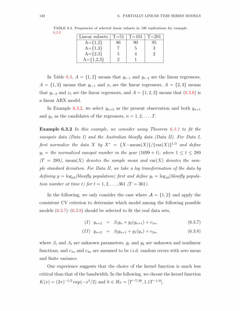
140 6. PARTIALLY LINEAR TIME SERIES MODELS
TABLE 6.3. Frequencies of selected linear subsets in 100 replications for example6.2.3
Linear subsets T=51 T=101 T=201A=1,2 86 90 95A=1,3 7 5 3A=2,3 5 4 2
A=1,2,3 2 1
In Table 6.3, A = 1, 2 means that yt−1 and yt−2 are the linear regressors,
A = 1, 3 means that yt−1 and xt are the linear regressors, A = 2, 3 means
that yt−2 and xt are the linear regressors, and A = 1, 2, 3 means that (6.3.6) is
a linear ARX model.
In Example 6.3.2, we select yn+2 as the present observation and both yn+1
and yn as the candidates of the regressors, n = 1, 2, . . . , T.
Example 6.3.2 In this example, we consider using Theorem 6.3.1 to fit the
sunspots data (Data I) and the Australian blowfly data (Data II). For Data I,
first normalize the data X by X∗ = X−mean(X)/var(X)1/2 and define
yt = the normalized sunspot number in the year (1699 + t), where 1 ≤ t ≤ 289
(T = 289), mean(X) denotes the sample mean and var(X) denotes the sam-
ple standard deviation. For Data II, we take a log transformation of the data by
defining y = log10(blowfly population) first and define yt = log10(blowfly popula-
tion number at time t) for t = 1, 2, . . . , 361 (T = 361).
In the following, we only consider the case where A = 1, 2 and apply the
consistent CV criterion to determine which model among the following possible
models (6.3.7)–(6.3.8) should be selected to fit the real data sets,
(I) yn+2 = β1yn + g2(yn+1) + e1n, (6.3.7)
(II) yn+2 = β2yn+1 + g1(yn) + e2n, (6.3.8)
where β1 and β2 are unknown parameters, g1 and g2 are unknown and nonlinear
functions, and e1n and e2n are assumed to be i.i.d. random errors with zero mean
and finite variance.
Our experience suggests that the choice of the kernel function is much less
critical than that of the bandwidth. In the following, we choose the kernel function
K(x) = (2π)−1/2 exp(−x2/2) and h ∈ HT = [T−7/30, 1.1T−1/6].

6. PARTIALLY LINEAR TIME SERIES MODELS 141
TABLE 6.4. The minimum CV values for example 6.3.1
Models CV–Data I CV–Data III 0.1914147 0.04251451II 0.1718859 0.03136296
Through computing the CV function defined by (6.3.2) for Example 6.3.2, we
can obtain the following minimum CV values listed in Table 6.4.
For the two data sets, when selecting yn+1 and yn as the candidates of the
regressors, Table 6.4 suggests using the prediction equation
yn+2 = β2(h2C)yn+1 + g1(yn), n = 1, 2, . . . , (6.3.9)
where g1(yn) = g2(yn, h2C)− β2(h2C)g1(yn, h2C) appears to be nonlinear,
gi(yn, h) = N∑m=1
K(yn − ym
h)ym+i
/ N∑m=1
K(yn − ym
h), i = 1, 2,
and h2C = 0.2666303 and 0.3366639, respectively.
In the following, we consider the case where A = 1, 2, 3 and apply the
consistent CV criterion to determine which model among the following possi-
ble models (6.3.10)–(6.3.15) should be selected to fit the real data sets given in
Examples 6.3.3 and 6.3.4 below,
(M1) Yt = β1Xt1 + β2Xt2 + g3(Xt3) + e1t, (6.3.10)
(M2) Yt = β3Xt1 + g2(Xt2) + β4Xt3 + e2t, (6.3.11)
(M3) Yt = g1(Xt1) + β5Xt2 + β6Xt3 + e3t, (6.3.12)
(M4) Yt = β7Xt1 +G1(X1t) + e4t, (6.3.13)
(M5) Yt = β8Xt2 +G2(X2t) + e5t, (6.3.14)
(M6) Yt = β9Xt3 +G3(X3t) + e6t, (6.3.15)
where X1t = (Xt2, Xt3)T , X2t = (Xt1, Xt3)T , X3t = (Xt1, Xt2)T , βi are unknown
parameters, (gj, Gj) are unknown and nonlinear functions, and eit are assumed
to be i.i.d. random errors with zero mean and finite variance.
Analogously, we can compute the corresponding CV functions with K and h
chosen as before for the following examples.
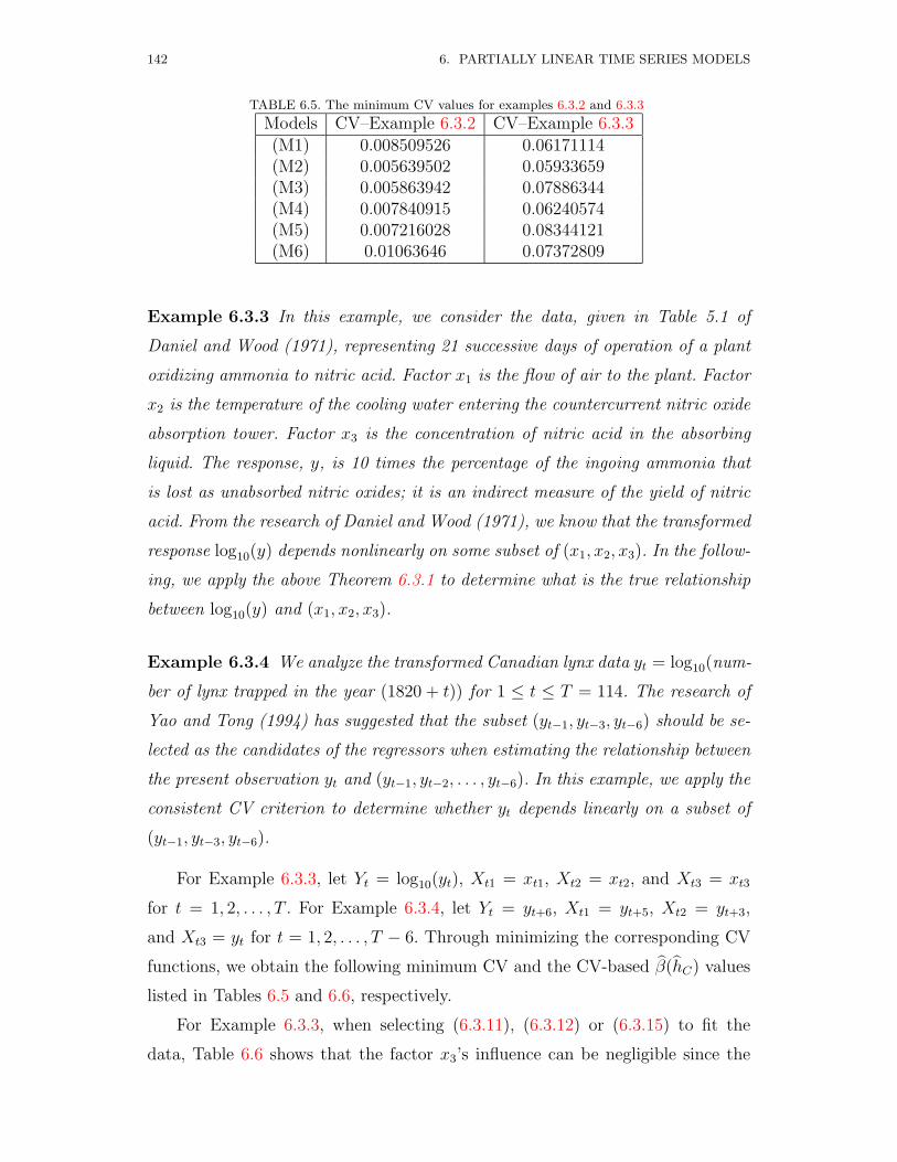
142 6. PARTIALLY LINEAR TIME SERIES MODELS
TABLE 6.5. The minimum CV values for examples 6.3.2 and 6.3.3
Models CV–Example 6.3.2 CV–Example 6.3.3(M1) 0.008509526 0.06171114(M2) 0.005639502 0.05933659(M3) 0.005863942 0.07886344(M4) 0.007840915 0.06240574(M5) 0.007216028 0.08344121(M6) 0.01063646 0.07372809
Example 6.3.3 In this example, we consider the data, given in Table 5.1 of
Daniel and Wood (1971), representing 21 successive days of operation of a plant
oxidizing ammonia to nitric acid. Factor x1 is the flow of air to the plant. Factor
x2 is the temperature of the cooling water entering the countercurrent nitric oxide
absorption tower. Factor x3 is the concentration of nitric acid in the absorbing
liquid. The response, y, is 10 times the percentage of the ingoing ammonia that
is lost as unabsorbed nitric oxides; it is an indirect measure of the yield of nitric
acid. From the research of Daniel and Wood (1971), we know that the transformed
response log10(y) depends nonlinearly on some subset of (x1, x2, x3). In the follow-
ing, we apply the above Theorem 6.3.1 to determine what is the true relationship
between log10(y) and (x1, x2, x3).
Example 6.3.4 We analyze the transformed Canadian lynx data yt = log10(num-
ber of lynx trapped in the year (1820 + t)) for 1 ≤ t ≤ T = 114. The research of
Yao and Tong (1994) has suggested that the subset (yt−1, yt−3, yt−6) should be se-
lected as the candidates of the regressors when estimating the relationship between
the present observation yt and (yt−1, yt−2, . . . , yt−6). In this example, we apply the
consistent CV criterion to determine whether yt depends linearly on a subset of
(yt−1, yt−3, yt−6).
For Example 6.3.3, let Yt = log10(yt), Xt1 = xt1, Xt2 = xt2, and Xt3 = xt3
for t = 1, 2, . . . , T . For Example 6.3.4, let Yt = yt+6, Xt1 = yt+5, Xt2 = yt+3,
and Xt3 = yt for t = 1, 2, . . . , T − 6. Through minimizing the corresponding CV
functions, we obtain the following minimum CV and the CV-based β(hC) values
listed in Tables 6.5 and 6.6, respectively.
For Example 6.3.3, when selecting (6.3.11), (6.3.12) or (6.3.15) to fit the
data, Table 6.6 shows that the factor x3’s influence can be negligible since the

6. PARTIALLY LINEAR TIME SERIES MODELS 143
TABLE 6.6. The CV-based β(hC) values for examples 6.3.2 and 6.3.3
β(hC)-Value Example 6.3.2 Example 6.3.4
β1(h1C) 0.01590177 0.9824141
β2(h1C) 0.0273703 -0.4658888
β3(h2C) 0.01744958 0.9403801
β4(h2C) -0.003478075 0.03612305
β5(h3C) 0.04129525 -0.4313919
β6(h3C) -0.001771901 0.02788928
β7(h4C) 0.01964107 0.9376097
β8(h5C) 0.04329919 -0.423475
β9(h6C) -0.003640449 0.03451025
CV-based coefficients β4(h2C), β6(h3C) and β9(h6C) are relatively smaller than
the other coefficients. This conclusion is the same as that of Daniel and Wood
(1971), who analyzed the data by using classical linear regression models. Table
6.5 suggests using the following prediction equation
yt = β3(h2C)xt1 + g2(xt2) + β4(h2C)xt3, t = 1, 2, . . . , 21,
where g2(xt2) = g2(xt2, h2C)−β3(h2C), β4(h2C)T g1(xt2, h2C) appears to be non-
linear,
gi(xt2, h) = 21∑s=1
K(xt2 − xs2
h)Zis
/ 21∑s=1
K(xt2 − xs2
h), i = 1, 2,
Z2s = Ys, Z1s = (xs1, xs2)T , and h2C = 0.6621739.
For the Canadian lynx data, when selecting yn+5, yn+3, and yn as the candi-
dates of the regressors, Tables 6.5 and 6.6 suggest using the following prediction
equation
yn+6 = β3(h2C)yn+5 + g2(yn+3) + β4(h2C)yn, n = 1, 2, . . . , 108, (6.3.16)
where g2(yn+3) = g2(yn+3, h2C)− β3(h2C), β4(h2C)T g1(yn+3, h2C) appears to be
nonlinear,
gi(yn+3, h) = 108∑m=1
K(ym+3 − yn+3
h)zim
/ 108∑m=1
K(ym+3 − yn+3
h), i = 1, 2,
z2m = ym+6, z1m = (ym+5, ym)T , and h2C = 0.3312498.
The research by Tong (1990) and Chen and Tsay (1993) has suggested that
the fully nonparametric autoregressive model of the form yt = g(yt−1, . . . , yt−r)+et

144 6. PARTIALLY LINEAR TIME SERIES MODELS
is easier to understand than the threshold autoregressive approach proposed by
Tong (1977). It follows from equations (6.3.9) and (6.3.16) that for the Cana-
dian lynx data, the sunspots data and the Australian blowfly data, the above
partially linear autoregressive model of the form (6.3.5) is more appro-
priate than the fully nonparametric autoregressive model.
6.4 Optimum Bandwidth Selection
6.4.1 Asymptotic Theory
As mentioned in Tong (1990), some nonlinear phenomena cannot be fitted by
linear ARMA models and therefore the fully nonparametric autoregressive func-
tion approach is recommended to use in practice. But in some cases, the fully
nonparametric autoregressive function approach will lose too much information
on the relationship between yt and yt−i, i ≥ 1 and neglect some existing lin-
ear dependencies among them. A reasonable approach to modelling the nonlinear
time series data is to use the partially linear additive autoregressive model
yt =p∑i=1
βiyt−ci +q∑j=1
gj(yt−dj) + et,
where t > max(cp, dq), 1 ≤ c1 < . . . < cp ≤ r, 1 ≤ d1 < . . . < dq ≤ r, and ci 6= dj
for all 1 ≤ i ≤ p and 1 ≤ j ≤ q.
There are a number of practical motivations for the study of the above model.
These include the research of population biology model and the Mackey-Glass sys-
tem (Glass and Mackey, 1988). Recently, Nychka, Elliner, Gallant and McCaffrey
(1992) suggested studying the model
yt = ayt−1 + byt−d
1 + ykt−d+ et.
For k = 10 this is a discretized version of the Mackey-Glass delay differential
equation, originally developed to model the production and loss of white blood
cells. It can also be interpreted as a model for population dynamics. If 0 < a < 1
and b > 0 and if yt denotes the number of adults, then a is the survival rate
of adults and d is the time delay between birth and maturation. The byt−d(1 +
ykt−d)−1 accounts for the recruitment of new adults due to births d years in
the past, which is non-linear because of decreased fecundity at higher population

6. PARTIALLY LINEAR TIME SERIES MODELS 145
levels. In addition, the development in partially linear (semiparametric) regression
has established a solid foundation for partially linear time series analysis.
For simplicity, we only consider a partially linear autoregressive model of the
form
yt = βyt−1 + g(yt−2) + et, t = 3, 4, . . . , T (6.4.1)
where β is an unknown parameter-of-interest, g is an unknown function over
R1 = (−∞,∞), et : t ≥ 3 is a sequence of i.i.d. random errors with Ee1 = 0
and Ee21 = σ2 <∞, and et : t ≥ 3 is independent of (y1, y2).
For identifiability, we assume that the (β, g) satisfies
Eyt − βyt−1 − g(yt−2)2 = min(α,f)
Eyt − αyt−1 − f(yt−2)2.
It follows from (6.4.1) that
g(yt−2) = E(yt − βyt−1)|yt−2
= E(yt|yt−2)− βE(yt−1|yt−2) = g1(yt−2)− βg2(yt−2).
The natural estimates of gi (i = 1, 2) and g can be defined by
g1,h(yt−2) =T∑s=3
Ws,h(yt−2)ys,
g2,h(yt−2) =T∑s=3
Ws,h(yt−2)ys−1,
and
gh(yt−2) = g1,h(yt−2)− βg2,h(yt−2),
where Ws,h(·) is a probability weight function depending on y1, y2, ..., yT−2 and
the number T of observations.
Based on the model yt = βyt−1 + gh(yt−2) + et, the kernel-weighted least
squares (LS) estimator β(h) of β can be defined by minimizing
T∑t=3
yt − βyt−1 − gh(yt−2)2.
We now obtain
β(h)− β =( T∑t=3
u2t
)−1 T∑t=3
utet +T∑t=3
utgh(yt−2), (6.4.2)

146 6. PARTIALLY LINEAR TIME SERIES MODELS
where ut = yt−1 − g2,h(yt−2) and gh(yt−2) = g(yt−2)− gh(yt−2).
In this section, we only consider the case where the Ws,h(·) is a kernel
weight function
Ws,h(x) = Kh(x− ys−2)/ T∑t=3
Kh(x− yt−2),
where Kh(·) = h−1K(·/h), K : R→ R is a kernel function satisfying Assumption
6.6.8 below and
h = hT ∈ HT = [a1T−1/5−c1 , b1T
−1/5+c1 ],
in which the absolute constants a1, b1 and c1 satisfy 0 < a1 < b1 < ∞ and
0 < c1 < 1/20.
A mathematical measurement of the proposed estimators can be obtained by
considering the average squared error (ASE)
D(h) =1
T − 2
T∑t=3
[β(h)yt−1 + g∗h(yt−2) − βyt−1 + g(yt−2)]2w(yt−2),
where g∗h(·) = g1,h(·)− β(h)g2,h(·) and w is a weight function. It follows from the
ASE (see Lemma 6.6.7 (i) below) that the theoretically optimum bandwidth is
proportional to n−1/5. Unfortunately, this optimization procedure has the draw-
back that it involves functionals of the underlying distribution. In this section, we
will propose a practical selection procedure and then discuss adaptive estimates.
We now have the main results of this section.
Theorem 6.4.1 Assume that Assumption 6.6.8 holds. Let Ee1 = 0 and Ee21 =
σ2 <∞. Then the following holds uniformly over h ∈ HT
√Tβ(h)− β −→L N(0, σ2σ−2
2 ),
where σ22 = Eyt−1 − E(yt−1|yt−2)2.
Theorem 6.4.2 Assume that Assumption 6.6.8 holds. Let Ee1 = 0 and Ee41 <
∞. Then the following holds uniformly over h ∈ HT
√Tσ(h)2 − σ2 −→L N(0, V ar(e2
1)),
where σ(h)2 = 1/T∑Tt=3yt − β(h)yt−12, yt−1 = yt−1 − g2,h(yt−2), and yt =
yt − g1,h(yt−2).
6. PARTIALLY LINEAR TIME SERIES MODELS 147
Remark 6.4.1 (i) Theorem 6.4.1 shows that the kernel-based estimator of β
is asymptotically normal with the smallest possible asymptotic variance (Chen
(1988)).
(ii) Theorems 6.4.1 and 6.4.2 only consider the case where et is a sequence
of i.i.d. random errors with Eet = 0 and Ee2t = σ2 < ∞. As a matter of fact,
both Theorems 6.4.1 and 6.4.2 can be modified to the case where Eet = 0 and
Ee2t = f(yt−1) with some unknown function f > 0. For this case, we need to
construct an estimator for f . For example,
fT (y) =T∑t=3
WT,t(y)yt − β(h)yt−1 − g∗h(yt−2)2,
where WT,t(y) is a kernel weight function, β(h) is as defined in (6.4.2) and
g∗h(yt−2) = g1,h(yt−2) − β(h)g2,h(yt−2). Similar to the proof of Theorem 6.4.1, we
can show that fT (y) is a consistent estimator of f . Then, we define a weighted
LS estimator β(h) of β by minimizing
T∑t=3
fT (yt−1)−1yt − βyt−1 − gh(yt−2)2,
where gh(yt−2) is as defined in (6.4.2).
Some additional conditions on f are required to establish the corresponding
results of Theorems 6.4.1 and 6.4.2.
Remark 6.4.2 A generalization of model (6.4.1) is
yt =p∑s=1
βsyt−s + g(yt−p−1) + et = xTt β + g(yt−p−1) + et, t ≥ p+ 2, (6.4.3)
where xt = (yt−1, . . . , yt−p)T , β = (β1, · · · , βp)T is a vector of unknown parameters,
and the g and et are as defined in (6.4.1). For this case, we need to modify the
above equations (see §4.2 of Chapter III of Gyorfi, Hardle, Sarda and Vieu (1989)
) and the kernel-weighted LS estimator of β can be defined as
β =( T∑t=p+2
UtUTt
)+T∑
t=p+2
UtVt,
where
Vt = yt − g0(yt−p−1), Ut = xt −G(yt−p−1),
G(·) = g1(·), . . . , gp(·)T , gi(·) =T∑
s=p+2
Ws,h(·)ys−i

148 6. PARTIALLY LINEAR TIME SERIES MODELS
for i = 0, 1, . . . , p, in which
Ws,h(·) = Kh(· − ys−p−1)/ T∑
l=p+2
Kh(· − yl−p−1).
Under similar conditions, the corresponding results of Theorems 6.4.1 and 6.4.2
can be established.
Remark 6.4.3 Theorems 6.4.1 and 6.4.2 only establish the asymptotic results
for the partially linear model (6.4.1). In practice, we need to determine whether
model (6.4.1) is more appropriate than
yt = f1(yt−1) + αyt−2 + εt, (6.4.4)
where f1 is an unknown function over R1, α is an unknown parameter and εt is
a sequence of i.i.d. random errors with mean zero and finite variance. In this case,
we need to modify the above estimation equations and to estimate the regression
function of E(yt−2|yt−1), which has been discussed in §5.2.4 of Tong (1990) and
Robinson (1983). They both have discussed the estimators of E(yt|yt±j) for j ≥ 1.
Therefore, similar results for (6.4.4) can also be obtained. Section 6.4.2 below
provides estimation procedures for both (6.4.1) and (6.4.4).
In the following section, we apply a cross-validation (CV) criterion to con-
struct an asymptotically optimal data-driven bandwidth and adaptive data-driven
estimates.
Let us define N = T − 2,
D(h) =1
T − 2
T∑t=3
[β(h)yt−1 + g∗h(yt−2) − βyt−1 + g(yt−2)]2w(yt−2)
=1
N
N∑n=1
[β(h)yn+1 + g∗h(yn) − βyn+1 + g(yn)]2w(yn), (6.4.5)
and
CV (h) =1
N
N∑n=1
[yn+2 − β(h)yn+1 + g1,n(yn)− β(h)g2,n(yn)]2w(yn), (6.4.6)
where β(h) is as defined in (6.4.2) with gh(·) replaced by gh,n(·) = g1,n(·)−βg2,n(·),in which
gi,n(·) = gi,n(·, h) =1
N − 1
∑m6=n
Kh(· − ym)ym+3−i/fh,n(·)
6. PARTIALLY LINEAR TIME SERIES MODELS 149
and
fh,n(·) =1
N − 1
∑m6=n
Kh(· − ym). (6.4.7)
Definition 6.4.1 A data-driven bandwidth h is asymptotically optimal if
D(h)
infh∈HT D(h)→p 1.
CROSS–VALIDATION (CV): Select h, denoted by hC , that achieves
CV (hC) = infh∈HN+2
CV (h). (6.4.8)
Theorem 6.4.3 Assume that the conditions of Theorem 6.4.1 hold. Then the
data-driven bandwidth hC is asymptotically optimal.
Theorem 6.4.4 Assume that the conditions of Theorem 6.4.1 hold. Then under
the null hypothesis H0 : β = 0
F1(hC) = Tβ(hC)2σ22σ−2 −→L χ2(1), (6.4.9)
as T →∞. Furthermore, under H1 : β 6= 0, we have F (hC)→∞ as T →∞.
Theorem 6.4.5 Assume that the conditions of Theorem 6.4.1 hold. Then under
the null hypothesis H ′0 : σ2 = σ20
F2(hC) = Tσ(hC)2 − σ202V ar(e2
1)−1 → χ2(1), (6.4.10)
as T →∞. Furthermore, under H ′1 : σ2 6= σ20, we have F (hC)→∞ as T →∞.
Remark 6.4.4 Theorems 6.4.3-6.4.5 show that the optimum data-driven band-
width hC is asymptotically optimal and the conclusions of Theorems 6.4.1 and
6.4.2 remain unchanged with h replaced by hC. It follows from Theorems 6.4.4
and 6.4.5 that when h is proportional to n−1/5, both β and σ2 are√n–consistent.
In addition, it follows from Lemma 6.6.7(i) that the nonparametric estimate g∗h
is of n−4/5 rate of mean squared error (MSE) when h is proportional to n−1/5.

150 6. PARTIALLY LINEAR TIME SERIES MODELS
6.4.2 Computational Aspects
In this subsection, we demonstrate how well the above estimation procedure works
numerically and practically.
Example 6.4.1 Consider model (6.4.1) given by
yt = βyt−1 + g(yt−2) + et, t = 3, 4, ..., T, (6.4.11)
where et : t ≥ 3 is independent and uniformly distributed over (−0.5, 0.5), y1
and y2 are mutually independent and identically distributed over (−1, 1), (y1, y2)
is independent of et : t ≥ 3, and (β, g) is chosen from one of the following
models.
Model 1. β = 0.25 and g(y) = y/2(1 + y2)−1.
Model 2. β = 0.25 and g(y) = 1/4 sin(πy).
In this section, we conduct a small sample study for the two models.
Choose the quartic kernel function
K(u) =
(15/16)(1− u2)2 if |u| ≤ 10 otherwise
and the weight function
w(x) =
1 if |x| ≤ 10 otherwise
First, because of the form of g, the fact that the process yt is strictly
stationary follows from §2.4 of Tjøstheim (1994) (also Theorem 3.1 of An and
Huang (1996)). Second, by using Lemma 3.4.4 and Theorem 3.4.10 of Gyorfi,
Hardle, Sarda and Vieu (1989). (also Theorem 7 of §2.4 of Doukhan (1995)), we
obtain that the yt is β-mixing and therefore α-mixing. Thus, Assumption 6.6.1
holds. Third, it follows from the definition of K and w that Assumption 6.6.8
holds.
(i). Based on the simulated data set yt : 1 ≤ t ≤ T, compute the following
estimators
g1,h(yn) = N∑m=1
Kh(yn − ym)ym+2
/ N∑m=1
Kh(yn − ym),
g2,h(yn) = N∑m=1
Kh(yn − ym)ym+1
/ N∑m=1
Kh(yn − ym),

6. PARTIALLY LINEAR TIME SERIES MODELS 151
gh(yn) = g1,h(yn)− 1
4g2,h(yn),
g1,n(yn) = N∑m6=n
Kh(yn − ym)ym+2
/ N∑m6=n
Kh(yn − ym),
g2,n(yn) = N∑m6=n
Kh(yn − ym)ym+1
/ N∑m6=n
Kh(yn − ym),
and
gn(yn) = g1,n(yn)− 1
4g2,n(yn), (6.4.12)
where Kh(·) = h−1K(·/h), h ∈ HN+2 = [(N + 2)−7/30, 1.1(N + 2)−1/6], and
1 ≤ n ≤ N .
(ii). Compute the LS estimates β(h) of (6.4.2) and β(h) of (6.4.6)
β(h)− β =( N∑n=1
u2n+2
)−1 N∑n=1
un+2en+2 +N∑n=1
un+2gh(yn)
(6.4.13)
and
β(h)− β =( N∑n=1
v2n+2
)−1 N∑n=1
vn+2en+2 +N∑n=1
vn+2gn(yn)
(6.4.14)
where un+2 = yn+1 − g2,h(yn), gh(yn) = g(yn) − gh(yn), vn+2 = yn+1 − g2,n(yn),
and gn(yn) = g(yn)− gn(yn).
(iii). Compute
D(h) =1
N
N∑n=1
mh(zn)−m(zn)2
=1
N
N∑n=1
[β(h)un+2 + g1,h(yn) − βyn+1 + g(yn)]2
=1
N
N∑n=1
β(h)un+2 + g1,h(yn)2
− 2
N
N∑n=1
β(h)un+2 + g1,h(yn)βyn+1 + g(yn)
+1
N
N∑n=1
βyn+1 + g(yn)2
≡ D1h +D2h +D3h, (6.4.15)
where the symbol “≡” indicates that the terms of the left-hand side can be
represented by those of the right-hand side correspondingly.

152 6. PARTIALLY LINEAR TIME SERIES MODELS
TABLE 6.7. Simulation results for model 1 in example 6.4.1
N | hC − hD | | β(hC)− 0.25 | | β(hC)− 0.25 | ASE(hC)100 0.08267 0.09821 0.09517 0.00451200 0.07478 0.07229 0.07138 0.00229300 0.08606 0.05748 0.05715 0.00108400 0.05582 0.05526 0.05504 0.00117500 0.07963 0.05025 0.05013 0.00076
Thus, D1h and D2h can be computed from (6.4.6)–(6.4.15). D3h is independent
of h. Therefore the problem of minimizing D(h) over HN+2 is the same as that
of minimizing D1h +D2h. That is
hD = arg minh∈HN+2
(D1h +D2h). (6.4.16)
(iv). Compute
CV (h) =1
N
N∑n=1
yn+2 − mh,n(zn)2
=1
N
N∑n=1
mh,n(zn)2 − 2
N
N∑n=1
mh,n(zn)yn+2 +1
N
N∑n=1
y2n+2
≡ CV (h)1 + CV (h)2 + CV (h)3. (6.4.17)
Hence, CV (h)1 and CV (h)2 can be computed by the similar reason as those
of D1h and D2h. Therefore the problem of minimizing CV (h) over HN+2 is the
same as that of minimizing CV (h)1 + CV (h)2. That is
hC = arg minh∈HN+2
CV (h)1 + CV (h)2. (6.4.18)
(v). Under the cases of T = 102, 202, 302, 402, and 502, compute
|hC − hD|, |β(hC)− β|, |β(hC)− β|, (6.4.19)
and
ASE(hC) =1
N
N∑n=1
g∗hC ,n
(yn)− g(yn)2. (6.4.20)
The following simulation results were performed 1000 times using the Splus
functions (Chambers and Hastie (1992)) and the means are tabulated in Tables
6.7 and 6.8.

6. PARTIALLY LINEAR TIME SERIES MODELS 153
TABLE 6.8. Simulation results for model 2 in example 6.4.1
N | hC − hD | | β(hC)− 0.25 | | β(hC)− 0.25 | ASE(hC)100 0.08952 0.07481 0.07367 0.05246200 0.08746 0.06215 0.06189 0.02635300 0.09123 0.05243 0.05221 0.01573400 0.09245 0.05138 0.05093 0.01437500 0.09561 0.05042 0.05012 0.01108
Remark 6.4.5 Table 6.7 gives the small sample results for the Mackey-Glass
system with (a, b, d, k) = (1/4, 1/2, 2, 2) (§4 of Nychka, Elliner, Gallant and Mc-
Caffrey (1992)). Table 6.8 provides the small sample results for Model 2 which
contains a sin function at lag 2. Trigonometric functions have been used in the
time series literature to describe periodic series. Both Tables 6.7 and 6.8 show that
when the bandwidth parameter was proportional to the reasonable candidate T−1/5,
the absolute errors of the data-driven estimates β(hC), β(hC) and ASE(hC) de-
creased as the sample size T increased, and |β(hC)−0.25| < |β(hC)−0.25| for all
the sample sizes. Thus, the CV -based hC and the adaptive data-driven estimator
β(hC) are recommended to use in practice.
Example 6.4.2 In this example, we consider the Canadian lynx data. This data
set is the annual record of the number of Canadian lynx trapped in the MacKenzie
River district of North-West Canada for the years 1821 to 1934. Tong (1977)
fitted an eleventh-order Gaussian autoregressive model to yt = log10(number of
lynx trapped in the year (1820 + t)) for t = 1, 2, ..., 114 (T = 114). It follows from
the definition of (yt, 1 ≤ t ≤ 114) that all the transformed values yt are bounded
by one.
Several models have already been used to fit the lynx data. Tong (1977)
proposed the eleventh-order Gaussian autoregressive model to fit the data. See
also Tong (1990). More recently, Wong and Kohn (1996) used a second-order
additive autoregressive model of the form
yt = g1(yt−1) + g2(yt−2) + et (6.4.21)
to fit the data, where g1 and g2 are smooth functions. The authors estimated
both g1 and g2 through using a Bayesian approach and their conclusion is that

154 6. PARTIALLY LINEAR TIME SERIES MODELS
the estimate of g1 is almost linear while the estimate of g2 is nonlinear. Their
research suggests that if we choose either model (6.4.22) or model (6.4.23) below
to fit the lynx data, model (6.4.22) will be more appropriate.
yt = β1yt−1 + g2(yt−2) + e1t, (6.4.22)
yt = g1(yt−1) + β2yt−2 + e2t, (6.4.23)
(6.4.24)
where β1 and β2 are unknown parameters, g1 and g2 are unknown functions, and
e1t and e2t are assumed to be i.i.d. random errors with zero mean and finite
variance.
Our experience suggests that the choice of the kernel function is much less
critical than that of the bandwidth . For Example 6.4.1, we choose the kernel
function K(x) = (2π)−1/2 exp(−x2/2), the weight function w(x) = I[1,4](x), h ∈H114 = [0.3·114−7/30, 1.1·114−1/6]. For model (6.4.22), similar to (6.4.6), we define
the following CV function (N = T − 2) by
CV1(h) =1
N
N∑n=1
(yn+2 − [β1(h)yn+1 + g1,n(yn)− β1(h)g2,n(yn)]
)2,
where
β1(h) = N∑n=1
v1,nw1,n
/ N∑n=1
v21,n
, v1,n = yn+1 − g2,n(yn),
w1,n = yn+2 − g1,n(yn),
gi,n(yn) = N∑m=1, 6=n
Kh(yn − ym)ym+3−i/ N∑
m=1, 6=nKh(yn − ym)
,
for i = 1, 2, and Kh(·) = 1/hK(·/h).
For model (6.4.23), we have
CV2(h) =1
N
N∑n=1
[yn+2 − gn,1(yn+1)− β2(h)gn,2(yn+1) + β2(h)yn]2,
where
β2(h) = N∑n=1
v2,nw2,n
/ N∑n=1
v22,n
, v2,n = yn − gn,2(yn+1),
w2,n = yn+2 − gn,1(yn+1),
gn,i(yn+1) = N∑m=1, 6=n
Kh(yn+1 − ym+1)ym+2i(2−i)/ N∑
m=1, 6=nKh(yn+1 − ym+1)

6. PARTIALLY LINEAR TIME SERIES MODELS 155
for i = 1, 2.
Through minimizing the CV functions CV1(h) and CV2(h), we obtain
CV1(h1C) = infh∈H114
CV1(h) = 0.0468 and CV2(h2C) = infh∈H114
CV2(h) = 0.0559
respectively. The estimates of the error variance of e1t and e2t were 0.04119
and 0.04643 respectively. The estimate of the error variance of the model of Tong
(1977) was 0.0437, while the estimate of the error variance of the model of Wong
and Kohn (1996) was 0.0421 which is comparable with our variance estimate
of 0.04119. Obviously, the approach of Wong and Kohn cannot provide explicit
estimates for f1 and f2 since their approach depends heavily on the Gibbs sampler.
Our CPU time for Example 6.4.2 took about 30 minutes on a Digital workstation.
Time plot of the common-log-transformed lynx data (part (a)), full plot of fitted
values (solid) and the observations (dashed) for model (6.4.22) (part (b)), partial
plot of the LS estimator (1.354yn+1) against yn+1 (part (c)), partial plot of the
nonparametric estimate (g2) of g2 in model (6.4.22) against yn (part (d)), partial
plot of the nonparametric estimate of g1 in model (6.4.23) against yn+1 (part (e)),
and partial plot of the LS estimator (−0.591yn) against yn (part (f)) are given
in Figure 6.1 on page 181. For the Canadian lynx data, when selecting yt−1 and
yt−2 as the candidates of the regressors, our research suggests using the following
prediction equation
yn+2 = 1.354yn+1 + g2(yn), n = 1, 2, . . . , (6.4.25)
where
g2(yn) = g1(yn, h1C)− 1.354g2(yn, h1C)
and
gi(yn, h) = N∑m=1
Kh(yn − ym)ym+3−i/ N∑
m=1
Kh(yn − ym),
in which i = 1, 2 and h1C = 0.1266. Part (d) of Figure 6.1 shows that g2 appears
to be nonlinear.
We now compare the methods of Tong (1977), Wong and Kohn (1996) and
our approach. The research of Wong and Kohn (1996) suggests that for the lynx
data, the second-order additive autoregressive model (6.4.25) is more reasonable

156 6. PARTIALLY LINEAR TIME SERIES MODELS
than the threshold autoregressive method proposed by Tong (1977). It follows
from (6.4.25) that for the lynx data the partially linear autoregressive model of
the form (6.4.1) is easier to implement in practice than the second-order additive
autoregressive model of Wong and Kohn (1996).
Remark 6.4.6 This section mainly establishes the estimation procedure for model
(6.4.1). As mentioned in Remarks 6.4.2 and 6.4.3, however, the estimation proce-
dure can be extended to cover a broad class of models. Section 6.4.2 demonstrates
that the estimation procedure can be applied to both simulated and real data ex-
amples. A software for the estimation procedure is available upon request. This
section shows that semiparametric methods can not only retain the beauty of lin-
ear regression methods but provide ’models’ with better predictive power than is
available from nonparametric methods.
6.5 Other Related Developments
In Sections 6.2–6.4, we have discussed the parametric and nonparametric tests,
the optimum linear subset selection and the optimal bandwidth parameter se-
lection for model (6.4.1). In this section, we summarize recent developments in a
general class of additive stochastic regression models including model (6.2.1).
Consider the following additive stochastic regression model
Yt = m(Xt) + et =p∑i=1
gi(Uti) + g(Vt) + et, (6.5.1)
where Xt = (UTt , V
Tt )T , Ut = (Ut1, . . . , Utp)
T , Vt = (Vt1, . . . , Vtd)T , and gi are un-
known functions on R1. For Yt = yt+r, Uti = Vti = yt+r−i and gi(Uti) = βiUti,
model (6.5.1) is a semiparametric AR model discussed in Section 6.2. For Yt =
yt+r, Uti = yt+r−i and g ≡ 0, model (6.5.1) is an additive autoregressive
model discussed extensively by Chen and Tsay (1993). Recently, Masry and
Tjøstheim (1995, 1997) discussed nonlinear ARCH time series and an additive
nonlinear bivariate ARX model, and proposed several consistent estimators. See
Tjøstheim (1994), Tong (1995) and Hardle, Lutkepohl and Chen (1997) for recent
developments in nonlinear and nonparametric time series models. Recently, Gao,
Tong and Wolff (1998a) considered the case where g ≡ 0 in (6.5.1) and discussed
the lag selection and order determination problem. See Tjøstheim and Auestad
(1994a, 1994b) for the nonparametric autoregression case and Cheng and Tong
6. PARTIALLY LINEAR TIME SERIES MODELS 157
(1992, 1993) for the stochastic dynamical systems case. More recently, Gao, Tong
and Wolff (1998b) proposed an adaptive test statistic for testing additivity
for the case where each gi in (6.5.1) is an unknown function in R1. Asymptotic
theory and power investigations of the test statistic have been discussed
under some mild conditions. This research generalizes the discussion of Chen, Liu
and Tsay (1995) and Hjellvik and Tjøstheim (1995) for testing additivity and
linearity in nonlinear autoregressive models. See also Kreiss, Neumann and
Yao (1997) for Bootstrap tests in nonparametric time series regression.
Further investigation of (6.5.1) is beyond the scope of this monograph. Recent
developments can be found in Gao, Tong and Wolff (1998a, b).
6.6 The Assumptions and the Proofs of Theorems
6.6.1 Mathematical Assumptions
Assumption 6.6.1 (i) Assume that et is a sequence of i.i.d. random pro-
cesses with Eet = 0 and Ee2t = σ2
0 <∞, and that es are independent of Xt
for all s ≥ t.
(ii) Assume that Xt are strictly stationary and satisfy the Rosenblatt mixing
condition
sup|P (A ∩B)− P (A)P (B)| : A ∈ Ωl1, B ∈ Ω∞l+k ≤ C1 exp(−C2k)
for all l, k ≥ 1 and for constants Ci > 0 : i = 1, 2, where Ωji denotes
the σ-field generated by Xt : i ≤ t ≤ j.
Let g(m) be the m-order derivative of the function g and M be a constant,
Gm(S) = g : |g(m)(s)− g(m)(s′)| ≤M ||s− s′||,
where m is an integer, s, s′ ∈ S, a compact subset of Rd, 0 < M <∞, and || · ||denotes the Euclidean norm.
Assumption 6.6.2 For g ∈ Gm(S) and zj(·) : j = 1, 2, . . . given above, there
exists a vector of unknown parameters γ = (γ1, . . . , γq)T such that for a constant
C0 (0 < C0 <∞) independent of T
q2(m+1)E q∑j=1
zj(Vt)γj − g(Vt)2∼ C0

158 6. PARTIALLY LINEAR TIME SERIES MODELS
where the symbol “∼” indicates that the ratio of the left-hand side and the right-
hand side tends to one as T → ∞, q = [l0T1
2(m+1)+1 ], in which 0 < l0 < ∞ is a
constant.
Assumption 6.6.3 (i) Z is of full column rank q, zi(·) : 1 ≤ i ≤ q is a
sequence of continuous functions with supv supi≥1 |zi(v)| <∞.
(ii) Assume that d2i = Ezi(Vt)2 exist with the absolute constants d2
i satisfying
0 < d21 ≤ · · · ≤ d2
q <∞ and that
Ezi(Vt)zj(Vt) = 0 and Ezk(Vs)zk(Vt) = 0
for all i 6= j, k ≥ 1 and s 6= t.
(iii) Assume that c2i = EU2
ti exist with the constants c2i satisfying 0 < c2
1 ≤· · · ≤ c2
p <∞ and that the random processes Ut : t ≥ 1 and zk(Vt) : k ≥1 satisfy the following orthogonality conditions
EUtiUtj = 0 and EUsiUtjzk(Vs)zk(Vt) = 0
for all i 6= j, k ≥ 1 and s 6= t.
Assumption 6.6.4 There exists an absolute constant M0 ≥ 4 such that for all
t ≥ 1
supxE|Yt − E(Yt|Xt)|2M0|Xt = x <∞.
Assumption 6.6.5 (i) Kd is a d–dimensional symmetric, Lipschitz continuous
probability kernel function with∫||u||2Kd(u)du <∞, and has an absolutely
integrable Fourier transform, where || · || denotes the Euclidean norm.
(ii) The distribution of Xt is absolutely continuous, and its density fX is bounded
below by cf and above by df on the compact support of fX .
(iii) The density function fV,A of random vector VtA has a compact support on
which all the second derivatives of fV,A, g1A and g2A are continuous, where
g1A(v) = E(Yt|VtA = v) and g2A(v) = E(UtA|VtA = v).

6. PARTIALLY LINEAR TIME SERIES MODELS 159
Assumption 6.6.6 The true regression function UTtA0βA0 +gA0(VtA0) is unknown
and nonlinear.
Assumption 6.6.7 Assume that the lower and the upper bands of HT satisfy
limT→∞
hmin(T, d)T 1/(4+d0)+c1 = a1 and limT→∞
hmax(T, d)T 1/(4+d0)−c1 = b1,
where d0 = r−|A0|, the constants a1, b1 and c1 only depend on (d, d0) and satisfy
0 < a1 < b1 <∞ and 0 < c1 < 1/4(4 + d0).
Assumption 6.6.8 (i) Assume that yt are strictly stationary and satisfy the
Rosenblatt mixing condition.
(ii) K is symmetric, Lipschitz continuous and has an absolutely integrable Fourier
transform.
(iii) K is a bounded probability kernel function with∫∞−∞ u
2K(u)du <∞.
(iv) Assume that the weight function w is bounded and that its support S is
compact.
(v) Assume that yt has a common marginal density f(·), f(·) has a compact
support containing S, and gi(·) (i = 1, 2) and f(·) have two continuous
derivatives on the interior of S.
(vi) For any integer k ≥ 1, E|yt|k <∞.
Remark 6.6.1 (i) Assumption 6.6.1(i) can be replaced by a more complicated
condition that includes the conditional heteroscedasticity case. Details can
be found in Gao, Tong and Wolff (1998b).
(ii) Assumption 6.6.1(ii) is quite common in such problems. See, for example,
(C.8) in Hardle and Vieu (1992). However, it would be possible, but with
more tedious proofs, to obtain the above Theorems under less restrictive
assumptions that include some algebraically decaying rates.
(iii) As mentioned before, Assumptions 6.6.2 and 6.6.3 provide some smooth
and orthogonality conditions. In almost all cases, they hold if g(·) satis-
fies some smoothness conditions. In particular, they hold when Assumption

160 6. PARTIALLY LINEAR TIME SERIES MODELS
6.6.1 holds and the series functions are either the family of trigonometric
series or the Gallant’s (1981) flexible Fourier form. Recent developments
in nonparametric series regression for the i.i.d. case are given in Andrews
(1991) and Hong and White (1995)
Remark 6.6.2 (i) Assumption 6.6.5(ii) guarantees that the model we consider
is identifiable, which implies that the unknown parameter vector βA0 and
the true nonparametric component gA0(VtA0) are uniquely determined up to
a set of measure zero.
(ii) Assumption 6.6.6 is imposed to exclude the case where gA0(·) is also a linear
function of a subset of Xt = (Xt1, . . . , Xtr)T .
(iii) Assumption 6.6.8 is similar to Assumptions 6.6.1 and 6.6.5. For the sake
of convenience, we list all the necessary conditions for Section 6.4 in the
separate assumption–Assumption 6.6.8.
6.6.2 Technical Details
Proof of Theorem 6.2.1
For simplicity, let Ci (0 < |Ci| < ∞) denote positive constants which may have
different values at each appearance throughout this section. Before proving The-
orem 6.2.1, we state a lemma, whose proof can be found in Lemma A.1 of Gao,
Tong and Wolff (1998a).
Lemma 6.6.1 Assume that the conditions of Theorem 6.2.1 hold. Then
c21 + oP (δ1(p)) ≤ λmin(
1
TUTU) ≤ λmax(
1
TUTU) ≤ c2
p + oP (δ1(p))
d21 + oP (λ2(q)) ≤ λmin(
1
TZTZ) ≤ λmax(
1
TZTZ) ≤ d2
q + oP (λ2(q))
where c2i = EU2
ti, and for all i = 1, 2, . . . , p and j = 1, 2, . . . , q
λi 1
TUTU − I1(p)
= oP (δ1(p)),
λj 1
TZTZ − I2(q)
= oP (λ2(q)),
where
I1(p) = diag(c21, . . . , c
2p) and I2(q) = diag(d2
1, . . . , d2q)

6. PARTIALLY LINEAR TIME SERIES MODELS 161
are p×p and q×q diagonal matrices respectively, λmin(B) and λmax(B) denote the
smallest and largest eigenvalues of matrix B, λi(D) denotes the i–th eigenvalue
of matrix D, and δ1(p) > 0 and λ2(q) > 0 satisfy as T →∞, maxδ1(p), λ2(q) ·maxp, q → 0 as T →∞.
The Proof of Theorem 6.2.1. Here we prove only Theorem 6.2.1(i) and the
second part follows similarly. Without loss of generality, we assume that the
inverse matrices (ZTZ)−1, (UTU)−1 and (UT U)−1 exist and that d21 = d2
2 = · · · =d2q = 1 and σ2
0 = 1.
By (6.2.7) and Assumption 6.6.2, we have
(ZTZ)1/2(γ − γ) = (ZTZ)−1/2ZTF − U(UT U)−1UT(e+ δ)
= (ZTZ)−1/2ZT e+ (ZTZ)−1/2ZT δ − (ZTZ)−1/2ZTU(UT U)−1UT e
−(ZTZ)−1/2ZTU(UT U)−1UT δ
≡ I1T + I2T + I3T + I4T , (6.6.1)
where e = (e1, . . . , eT )T , δ = (δ1, . . . , δT )T , and δt = g(Vt)− Z(Vt)Tγ.
In view of (6.6.1), in order to prove Theorem 6.2.1, it suffices to show that
(2q)−1/2(eTPe− q) −→L N(0, 1) (6.6.2)
and for i = 2, 3, 4
IT1T IiT = oP (q1/2) and ITiT IiT = oP (q1/2). (6.6.3)
Before proving (6.6.2), we need to prove
eTPe =∑
1≤s,t≤Tasteset + oP (q1/2), (6.6.4)
where ast = 1/T∑qi=1 zi(Vs)zi(Vt).
In order to prove (6.6.4), it suffices to show that
q−1/2|eT (P − P0)e| = oP (1), (6.6.5)
where P0 = ast1≤s,t≤T is a matrix of order T × T .
Noting that Lemma 6.6.1 holds and∣∣∣eTZ(ZTZ)−1I2(q) − 1
TZTZI2(q)−1ZT e
∣∣∣∣2≤ eTZ(ZTZ)−1ZT e
× eTZI2(q)− 1
TZTZ(ZTZ)−1I2(q)− 1
TZTZZT e
≤ C
T 2λmax(I2(q)− 1
TZTZ)2(eTZZT e)2,

162 6. PARTIALLY LINEAR TIME SERIES MODELS
in order to prove (6.6.5), it suffices to show that
λ2(q)T−1q−1/2(ZT e)T (ZT e) = oP (1), (6.6.6)
which follows from Markov inequality and
Pλ2(q)T−1q−1/2(ZT e)T (ZT e) > ε ≤ ε−1λ2(q)T−1q−1/2Eq∑i=1
T∑t=1
zi(Vt)et2
≤ Cλ2(q)T−1q−1/2qT
= Cλ2(q)q1/2 = o(1)
using Assumptions 6.6.1 and 6.6.3. Thus, the proof of (6.6.4) is completed.
Noting (6.6.4), in order to prove (6.6.2), it suffices to show that as T →∞
q−1/2( T∑t=1
atte2t − q
)−→P 0 (6.6.7)
and
T∑t=2
WTt −→L N(0, 1), (6.6.8)
where WTt = (2/q)1/2∑t−1s=1 asteset forms a zero mean martingale difference.
Now applying a central limit theorem for martingale sequences (see Theorem
1 of Chapter VIII of Pollard (1984)), we can deduce
T∑t=2
WTt −→L N(0, 1)
if
T∑t=2
E(W 2Tt|Ωt−1) −→P 1 (6.6.9)
and
T∑t=2
EW 2TtI(|WTt| > c)|Ωt−1 −→P 0 (6.6.10)
for all c > 0.
It is obvious that in order to prove (6.6.9) and (6.6.10), it suffices to show
that as T →∞
2
q
T∑t=2
t−1∑s=1
a2ste
2s − 1 −→P 0, (6.6.11)
2
q
T∑t=1
∑r 6=s
astarteser −→P 0, (6.6.12)
6. PARTIALLY LINEAR TIME SERIES MODELS 163
and
4
q2
T∑t=2
E
(t−1∑s=1
astes
)4
→ 0. (6.6.13)
The left-hand side of (6.6.11) is
2
q
T∑t=2
t−1∑s=1
a2st(e
2s − 1) +
(2
q
T∑t=2
t−1∑s=1
a2st − 1
). (6.6.14)
Also, the first term in (6.6.14) is
2
q
q∑i=1
1
T
T∑t=2
zi(Vt)2 × 1
T
t−1∑s=1
zi(Vs)2(e2
s − 1)
+2
q
q∑i6=j=1
1
T 2
T∑t=2
t−1∑s=1
fij(Vs, Vt)(e2s − 1)
≡ 2
q
q∑i=1
1
T
T∑t=2
zi(Vt)2 ·M1t(i)
+
2
q
q∑i=1
q∑j=1, 6=i
M1ij, (6.6.15)
where fij(Vs, Vt) = zi(Vs)zj(Vs)zi(Vt)zj(Vt).
The second term in (6.6.14) is
1
q
q∑i=1
[ 1
T
T∑t=1
zi(Vt)2 − 1
2+ 2
1
T
T∑t=1
zi(Vt)2 − 1
]
+1
q
q∑i=1
q∑j=1, 6=i
1
T 2
T∑t=1
T∑s=1
zi(Vs)zj(Vs)zi(Vt)zj(Vt)
≡ 1
q
q∑i=1
Mi +1
q
q∑i=1
q∑j=1, 6=i
M2ij. (6.6.16)
Analogously, the left-hand side of (6.6.12) is
4
q
q∑i=1
1
T
T∑t=2
zi(Vt)2 × 1
T
t−1∑r=2
r−1∑s=1
zi(Vs)zi(Vr)eser
+4
q
q∑i=1
q∑j=1, 6=i
1
T 2
T∑t=2
t−1∑r=2
r−1∑s=1
gij(Vs, Vr, Vt)
≡ 4
q
q∑i=1
1
T
T∑t=2
zi(Vt)2 ·M2t(i) +
4
q
q∑i=1
q∑j=1, 6=i
M3ij, (6.6.17)
where gij(Vs, Vr, Vt) = zi(Vs)eszj(Vr)erzi(Vt)zj(Vt).
Using Assumptions 6.6.1-6.6.3 and applying the martingale limit results of
Chapters 1 and 2 of Hall and Heyde (1980), we can deduce for i = 1, 2, j = 1, 2, 3
and s, r ≥ 1
Ms = oP (1), Mjsr = oP (q−1),

164 6. PARTIALLY LINEAR TIME SERIES MODELS
and
max1≤t≤T
|Mit(s)| = oP (1). (6.6.18)
Thus, equations (6.6.11) and (6.6.12) follows from (6.6.14)–(6.6.18). Now, we
begin to prove (6.6.13). Obviously,
(t−1∑s=1
astes)4
=1
T 4
q∑i=1
t−1∑s=1
zi(Vs)eszi(Vt)4≤ Cq3
T 4
q∑i=1
t−1∑s=1
zi(Vs)es4
(6.6.19)
using Assumption 6.6.3(i).
For any fixed i ≥ 1
T∑t=2
Et−1∑s=1
zi(Vs)es4
= C1
T∑t=2
t−1∑s=1
Ezi(Vs)es4
+C2
T∑t=2
t−1∑s1=1
t−1∑s2=1, 6=s1
Ezi(Vs1)2e2s1zi(Vs2)2e2
s2
≡ Ji1T + Ji2T .
Applying Assumptions 6.6.1(i) and 6.6.3(iii) again, we have for j = 1, 2
JijT ≤ C3T3. (6.6.20)
Thus, (6.6.19)–(6.6.20) imply (6.6.13). We have therefore proved equations (6.6.11)
–(6.6.13). As a result, equation (6.6.8) holds. In the following, we begin to prove
(6.6.7).
For any 1 ≤ i ≤ q, define
φii =1
T
T∑t=1
zi(Vt)2 − 1.
Using Assumptions 6.6.1 and 6.6.3, and applying Lemma 3.2 of Boente and
Fraiman (1988), we have for any given ε > 0
P (max1≤i≤q
|φii| > εq−1/2) ≤q∑i=1
P (|φii| > εq−1/2)
≤ C1q exp(−C2T1/2q−1/2)→ 0
as T →∞, where Ci are constants.
Thus
max1≤i≤q
|φii| = oP (q−1/2).

6. PARTIALLY LINEAR TIME SERIES MODELS 165
Therefore, using Assumptions 6.6.1 and 6.6.3, and applying Cauchy-Schwarz in-
equality, we obtain
T∑t=1
atte2t − q =
T∑t=1
att(e2t − 1) + tr[Z1/TI2(q)−1ZT − P ]
=T∑t=1
att(e2t − 1) + tr[I2(q)−11/TZTZ − I2(q)]
=T∑t=1
att(e2t − 1) +
q∑i=1
φii = oP (q1/2),
where tr(B) denotes the trace of matrix B.
The proof of (6.6.2) is consequently completed. Before proving (6.6.3), we
need to prove for T large enough
λmax(1
TZZT ) = oP (q−1/2),
which follows from
P∣∣∣ T∑t=1
T∑s=1
q∑i=1
zi(Vs)zi(Vt)lslt∣∣∣ > εTq−1/2
≤ q1/2
TεE∣∣∣ T∑t=1
T∑s=1
q∑i=1
zi(Vs)zi(Vt)lslt∣∣∣
≤ Cq1/2
T
q∑i=1
E∣∣∣ T∑t=1
T∑s=1
zi(Vs)zi(Vt)lslt∣∣∣
= Cq1/2
T
q∑i=1
E T∑t=1
zi(Vt)lt2≤ C
q3/2
T→ 0
using Assumption 6.6.3(ii) and the fact that l = (l1, . . . , lT )T is any identical
vector satisfying∑Tt=1 l
2t = 1. Thus
δTPδ ≤ λmax(ZTZ)−1δTZZT δ ≤ C
Tλmax(ZZT )δT δ = oP (q1/2).
We now begin to prove
IT3T I3T = oP (q1/2).
It is obvious that
IT3T I3T = eT U(UT U)−1UTPU(UT U)−1UT e
≤ λmax(UTPU) · λmax(UT U)−1 · eT U(UT U)−1UT e
≤ C
Tλmax(ZTZ)−1λmax(UTZZTU)eT U(UT U)−1UT e. (6.6.21)

166 6. PARTIALLY LINEAR TIME SERIES MODELS
Similar to the proof of (6.6.4), we can prove
eT U(UT U)−1UT e = C1p+ oP (p1/2) (6.6.22)
using Assumptions 6.6.2 and 6.6.3.
In order to estimate the order of (6.6.21), it suffices to estimate
λmax
1
T(ZTU)T (ZTU)
.
Analogous to the proof of Lemma 6.6.1, we have for 1 ≤ i ≤ p
λi 1
T(ZTU)T (ZTU)
≤ 2p max
1≤i6=j≤p|dij| = oP (ε(p)Tq), (6.6.23)
where
dij =1
T
q∑l=1
T∑s=1
Usizl(Vs) T∑
t=1
Utjzl(Vt)
denote the (i, j) elements of the matrix 1/T (ZTU)T (ZTU) and ε(p) satisfies
ε(p)→ 0
as T →∞.
Therefore, equations (6.6.21), (6.6.22) and (6.6.23) imply
IT3T I3T ≤ oP (ε(p)qp) = oP (q1/2)
when ε(p) = (p√q)−1.
Analogously, we can prove the rest of (6.6.2) similarly and therefore we finish
the proof of Theorem 6.2.1(i).
Proofs of Theorems 6.3.1 and 6.3.2
Technical lemmas
Lemma 6.6.2 Assume that Assupmtions 6.3.1, 6.6.1, and 6.6.4-6.6.6 hold,
limT→∞
maxdhmin(T, d) = 0 and lim
T→∞mindhmax(T, d)T 1/(4+d) =∞.
Then
limT→∞
Pr(A0 ⊂ A0) = 1.

6. PARTIALLY LINEAR TIME SERIES MODELS 167
Lemma 6.6.3 Under the conditions of Theorem 6.3.1, we have for every given
A
CV (A) = infh∈HT
CV (h,A) = σ2T + C1(A)T−4/(4+d) + oP (T−4/(4+d)), (6.6.24)
where σ2T = 1/T
∑Tt=1 e
2t and C1(A) is a positive constant depending on A.
The following lemmas are needed to complete the proof of Lemmas 6.6.2 and
6.6.3.
Lemma 6.6.4 Under the conditions of Lemma 6.6.2, we have for every given A
and any given compact subset G of Rd
suph∈HT
supv∈G||g1(v;h,A)− g1A0(v)|| = oP (T−1/4),
suph∈HT
supv∈G|g2(v;h,A)− g2A0(v)| = oP (T−1/4),
suph∈HT
supv∈G|f(v;h,A)− fA0(v)| = oP (T−1/4).
where gi and f are defined in (6.3.3) and (6.3.4).
Proof. The proof of Lemma 6.6.4 follows similarly from that of Lemma 1 of
Hardle and Vieu (1992).
Lemma 6.6.5 Under the conditions of Lemma 6.6.2, for every given A, the fol-
lowing holds uniformly over h ∈ HT
β(h,A)− βA0 = OP (T−1/2). (6.6.25)
Proof. The proof of (6.6.25) follows directly from the definition of β(h,A) and
the conditions of Lemma 6.6.5.
Proofs of Lemmas 6.6.2 and 6.6.3
Let
D1(h,A) =1
T
T∑t=1
g1t(VtA, h)− g1A0(VtA0)2,
D2(h,A) =1
T
T∑t=1
g2t(VtA, h)− g2A0(VtA0)g2t(VtA, h)− g2A0(VtA0)T ,
where g1A0(VtA0) = E(Yt|VtA0) and g2A0(VtA0) = E(UtA0|VtA0).

168 6. PARTIALLY LINEAR TIME SERIES MODELS
Obviously,
D(h,A) =1
T
T∑t=1
UTtAβ(h,A)− UT
tA0βA02+
1
T
T∑t=1
gt(VtA, β(h,A))− gA0(VtA0)2
− 2
T
T∑t=1
UTtAβ(h,A)− UT
tA0βA0gt(VtA, β(h,A))− gA0(VtA0)
≡ D1(h,A) +D2(h,A) +D3(h,A).
Similarly, we can prove
D2(h,A) = D1(h,A) + βTA0D2(h,A)βA0 + oP (D2(h,A)).
and for i = 1, 3 and every given A ⊂ A
suph∈HT
Di(h,A)
D2(h,A)= oP (1).
From the definition of CV (h,A), we have
CV (h,A) =1
T
T∑t=1
Yt − UTtAβ(h,A)− gt(VtA, β(h,A))2
=1
T
T∑t=1
e2t +D(h,A) +R(h,A), (6.6.26)
where
R(h,A) =2
T
T∑t=1
[UTtA0βA0 + gA0(VtA0) − UT
tAβA + gt(VtA, β(h,A))]et
satisfies for every given A ⊂ A
suph∈HT
R(h,A)
D(h,A)= oP (1).
Thus, we have for every given h ∈ HT and A ⊂ A
CV (h,A) =1
T
T∑t=1
e2t +D(h,A) + oP (D(h,A)).
In order to prove Lemma 6.6.2, it suffices to show that there exists a h∗ ∈ HT
such that for any h ∈ HT , A 6= A0 and A ⊂ A− A0
CV (h∗, A0) < CV (h,A),
which can be proved by comparing the corresponding terms of CV (h,A0) and
CV (h,A). The detail is similar to the proof of Theorem 1 of Chen and Chen
(1991). Thus, the proof of Lemma 6.6.2 is finished.

6. PARTIALLY LINEAR TIME SERIES MODELS 169
According to Lemma 6.6.2, we need only to consider those A satisfying
A ⊂ A0 and A 6= A0. Under the conditions of Lemma 6.6.2, we can show
that there exist two constants C0(A) and C1(A) depending on A such that
h∗d = C0(A)T−1/(4+d) ∈ HT and for every given A ⊂ A
CV (A) = infh∈HT
CV (h,A) = CV (h∗d, A)
= σ2T + C1(A)T−4/(4+d) + oP (T−4/(4+d)). (6.6.27)
which implies Lemma 6.6.3. The proof of (6.6.27) is similar to that of Lemma 8
of Hardle and Vieu (1992).
Proof of Theorem 6.3.1
According to Lemma 6.6.2 again, we only need to consider those A satisfying
A ⊂ A0 and A 6= A0. Thus, by (6.6.24) we have as T →∞
PrCV (A) > CV (A0) = PrC1(A)T
4(d−d0)
(4+d)(4+d0)
−C1(A0) + oP (T4(d−d0)
(4+d)(4+d0) ) > 0→ 1. (6.6.28)
Equation (6.6.28) implies limT→∞ Pr(A0 = A0) = 1 and therefore we complete
the proof of Theorem 6.3.1.
Proof of Theorem 6.3.2
Analogous to (6.6.26), we have
σ(h, A0)2 =1
T
T∑t=1
Yt − UTtA0β(h, A0)− g(V
tA0, h)2
=1
T
T∑t=1
e2t +
1
T
T∑t=1
UTtA0βA0 − UT
tA0β(h, A0)2
+1
T
T∑t=1
gA0(VtA0)− g(VtA0, h)2+
2
T
T∑t=1
UTtA0βA0 − UT
tA0β(h, A0)et
+2
T
T∑t=1
UTtA0βA0 − UT
tA0β(h, A0)gA0(VtA0)− g(V
tA0, h)
+2
T
T∑t=1
gA0(VtA0)− g(VtA0, h)et
≡ 1
T
T∑t=1
e2t + ∆(h, A0).
It follows that as T →∞
1
T
T∑t=1
e2t −→P σ
20. (6.6.29)

170 6. PARTIALLY LINEAR TIME SERIES MODELS
By applying Lemmas 6.6.4 and 6.6.5, it can be shown that
∆(h, A0) −→P 0. (6.6.30)
Therefore, the proof of Theorem 6.3.2 follows from (6.6.29) and (6.6.30).
Proofs of Theorems 6.4.1-6.4.5
Technical Lemmas
Lemma 6.6.6 Assume that Assumption 6.6.8 holds. Then as T →∞
supx
suph∈HT
|fh(x)− f(x)| = oP (1),
where the supx is taken over all values of x such that f(x) > 0 and
fh(·) =1
T − 2
T∑t=3
Kh(· − yt−2).
Proof. Lemma 6.6.6 is a weaker version of Lemma 1 of Hardle and Vieu (1992).
Lemma 6.6.7 (i) Assume that Assumption 6.6.8 holds. Then there exists a se-
quence of constants Cij : 1 ≤ i ≤ 2, 1 ≤ j ≤ 2 such that
Li(h) =1
N
N∑n=1
gi,h(yn)− gi(yn)2w(yn)
= Ci11
Nh+ Ci2h
4 + oP (Li(h)), (6.6.31)
Mi(h) =1
N
N∑n=1
gi,h(yn)− gi(yn)Zn+2w(yn) = oP (Li(h)) (6.6.32)
uniformly over h ∈ HT , where Zn+2 = yn+1 − E(yn+1|yn).
(ii) Assume that Assumption 6.6.8 holds. Then for i = 1, 2
suph∈HT
1
N
N∑n=1
gi,h(yn)− gi(yn)2 = oP (N−1/2), (6.6.33)
suph∈HT
1
N
N∑n=1
gi,h(yn)− gi(yn)Zn+2 = oP (N−1/2). (6.6.34)
Proof. (i) In order to prove Lemma 6.6.7, we need to establish the following fact
gi,h(yn)− gi(yn) = gi,h(yn)− gi(yn) fh(yn)
f(yn)
+gi,h(yn)− gi(yn)f(yn)− fh(yn)
f(yn). (6.6.35)

6. PARTIALLY LINEAR TIME SERIES MODELS 171
Note that by Lemma 6.6.6, the second term is negligible compared to the first.
Similar to the proof of Lemma 8 of Hardle and Vieu (1992), replacing Lemma 1
of Hardle and Vieu (1992) by Lemma 6.6.6, and using (6.6.35), we can obtain the
proof of (6.6.31). Using the similar reason as in the proof of Lemma 2 of Hardle
and Vieu (1992), we have for i = 1, 2
Li(h) =1
N
N∑n=1
gi,h(yn)− gi,n(yn)2w(yn) = oP (Li(h)). (6.6.36)
It follows from (6.4.7) that for i = 1, 2
1
N
N∑n=1
gi,h(yn)− gi(yn)Zn+2w(yn) =1
N
N∑n=1
gi,n(yn)− gi(yn)Zn+2w(yn)
+1
N
N∑n=1
gi,h(yn)− gi,n(yn)Zn+2w(yn),
where
gi,h(yn)− gi,n(yn) =K(0)(Nh)−1yn+3−i − gi,h(yn)
fh(yn)− (Nh)−1K(0). (6.6.37)
Observe that
yn+2 − g1,h(yn) = en+2 + βun+2 + g1(yn)− g1,h(yn)− βg2(yn)− g2,h(yn)
and
yn+1 − g2,h(yn) = un+2 = Zn+2 + g2(yn)− g2,h(yn). (6.6.38)
In order to prove (6.6.32), in view of (6.6.36)–(6.6.38), it suffices to show that
for i = 1, 2
1
N
N∑n=1
gi,n(yn)− gi(yn)Zn+2w(yn) = oP (Li(h)) (6.6.39)
and
1
N
N∑n=1
gi,h(yn)− gi,n(yn)Zn+2w(yn) = oP (Li(h)). (6.6.40)
The proof of (6.6.39) follows from that of (5.3) of Hardle and Vieu (1992).
The proof of (6.6.40) follows from Cauchy-Schwarz inequality, (6.6.36)–(6.6.38),
Lemma 6.6.6, (6.6.31) and
1
N
N∑n=1
Z2n+2w(yn) = OP (1), (6.6.41)

172 6. PARTIALLY LINEAR TIME SERIES MODELS
which follows from the fact that w is bounded and
1
N
N∑n=1
Z2n+2 →P σ
22 (6.6.42)
using the standard ergodic theorem, where
σ22 = Eyn+1 − E(yn+1|yn)2
= Ey2n+1 − EE2(yn+1|yn) ≤ 2Ey2
n+1 <∞
using Assumption 6.6.8(vi).
(ii) Lemma 6.6.7(ii) is a weaker version of Lemma 6.6.7(i). Similar to the
proof of Lemma 8 of Hardle and Vieu (1992) and the proof of (5.3) of Hardle
and Vieu (1992), and using the fact that Assumption 6.6.8 still holds when the
compact support of the weight function w is the same as that of the density f ,
we can prove both (6.6.33) and (6.6.34).
Lemma 6.6.8 Let Znk, k ≥ 0 be a sequence of random variables and Ωn,k−1be an increasing sequence of σ-fields such that Znk is measurable with respect
to Ωnk, and E(Znk|Ωn,k−1) = 0 for 1 ≤ k ≤ n. If as n→∞,
(i)∑nk=1 E(Z2
nk|Ωn,k−1)→ a22(> 0) in probability;
(ii) for every b2 > 0, the sum∑nk=1 EZ2
nkI(|Znk| > b2)|Ωn,k−1 converges in
probability to zero; then as n→∞n∑k=1
Znk −→L N(0, a22).
Proof. See Theorem 1 of Chapter VIII in Pollard (1984).
Lemma 6.6.9 Assume that Assumption 6.6.8 holds. Then
limT→∞
1
Tsuph∈HT
T∑t=3
u2t = σ2
2 (6.6.43)
in probability.
Proof. Observe that
1
T
T∑t=3
u2t =
1
T
T∑t=3
Z2t +
1
T
T∑t=3
(g22t,h + 2g2t,hZt)
≡ 1
T
T∑t=3
Z2t +RT (h),
6. PARTIALLY LINEAR TIME SERIES MODELS 173
where g2t,h = g2(yt−2)− g2,h(yt−2) and
RT (h) =1
T
T∑t=3
g2(yt−2)− g2,h(yt−2)2
+2
T
T∑t=3
g2(yt−2)− g2,h(yt−2)yt−1 − E(yt−1|yt−2)
≡ R1T (h) +R2T (h).
In view of (6.6.42), in order to prove (6.6.43), it suffices to show that for
i = 1, 2
suph∈HT
RiT (h) = oP (1),
which follows from Lemma 6.6.7(ii).
Proofs of Theorems 6.4.1 and 6.4.4
By (6.4.2), in order to prove Theorem 6.4.1, it suffices to show that as T →∞
T−1/2T∑t=3
Ztet −→L N(0, σ2σ−22 ), (6.6.44)
T∑t=3
g2,h(yt−2)− g2(yt−2)et = oP (T 1/2), (6.6.45)
T∑t=3
gh(yt−2)− g(yt−2)Zt = oP (T 1/2), (6.6.46)
and
T∑t=3
g2,h(yt−2)− g2(yt−2)gh(yt−2)− g(yt−2) = oP (T 1/2) (6.6.47)
uniformly over h ∈ HT , where
g(yt−2)− gh(yt−2) = g1(yt−2)− g1,h(yt−2)− βg2(yt−2)− g2,h(yt−2). (6.6.48)
Write Ωt+1 for the σ-field generated by y1, y2; e3, · · · , et. The variable Ztetis a martingale difference for Ωt.
By (6.6.42) we have as T →∞
1
T
T∑t=3
E(Ztet)2|Ωt →P σ2σ2
2. (6.6.49)

174 6. PARTIALLY LINEAR TIME SERIES MODELS
Observe that for every given b2 > 0
1
T
T∑t=3
E(Ztet)2I(|Ztet| > b2T1/2)|Ωt
≤ 1
T
T∑t=3
E(Ztet)2I(e2t > b2T
1/2)|Ωt+1
T
T∑t=3
E(Ztet)2I(Z2t > b2T
1/2)|Ωt
=1
T
T∑t=3
Z2tEe
2t I(e2
1 > b2T1/2) +
1
T
T∑t=3
Z2t σ
2I(Z2t > b2T
1/2). (6.6.50)
Because of (6.6.42), the first sum converges to zero in probability. The second
sum converges in L1 to zero because of Assumption 6.6.8. Thus, by Lemma 6.6.8
we obtain the proof of (6.6.45).
The proofs of (6.6.45) and (6.6.46) follow from (6.6.34). The proof of (6.6.47)
follows from (6.6.33) and Cauchy-Schwarz inequality. The proof of Theorem 6.4.4
follows immediately from that of Theorem 6.4.1 and the fact that hC ∈ HT defined
in (6.4.8).
Proofs of Theorems 6.4.2 and 6.4.5
In order to complete the proof of Theorem 6.4.2, we first give the following de-
composition of σ(h)2
σ(h)2 =1
T
T∑t=3
yt − β(h)yt−1 − g∗h(yt−2)2
=1
T
T∑t=3
e2t +
1
T
T∑t=3
u2tβ − β(h)2 +
1
T
T∑t=3
g2t,h
+2
T
T∑t=3
etutβ − β(h)+2
T
T∑t=3
etgt,h +2
T
T∑t=3
gt,hutβ − β(h)
≡6∑j=1
Jjh, (6.6.51)
where gt,h = g(yt−2)− gh(yt−2).
By (6.6.42) and Theorem 6.4.1 we have
suph∈HT
|J2h| ≤ oP (T−1/2). (6.6.52)
Also, by (6.6.48) and Lemma 6.6.7(ii) we get
suph∈HT
|J3h| ≤ oP (T−1/2). (6.6.53)

6. PARTIALLY LINEAR TIME SERIES MODELS 175
Similar to the proof of (6.6.34), we obtain for i = 1, 2
1
T
T∑t=3
etgi,h(yt−2)− gi(yt−2) ≤ oP (T−1/2) (6.6.54)
uniformly over h ∈ HT .
By Theorem 6.4.1, Lemma 6.6.7(ii), (6.6.48) and (6.6.52) we have
J4h =2
Tβ − β(h)
[ T∑t=3
etZt +T∑t=3
etg2(yt−2)− g2,h(yt−2)]
= oP (T−1/2), (6.6.55)
J5h =2
T
T∑t=3
etg(yt−2)− gh(yt−2) = oP (T−1/2), (6.6.56)
and
J6h =2
Tβ − β(h)
T∑t=3
utg(yt−2)− gh(yt−2)
=2
Tβ − β(h)
T∑t=3
Ztg(yt−2)− gh(yt−2)
+2
Tβ − β(h)
T∑t=3
Ztg(yt−2)− gh(yt−2)g2(yt−2)− g2,h(yt−2)
= oP (T−1/2) (6.6.57)
using the Cauchy-Schwarz inequality.
Therefore, the proof of Theorem 6.4.2 follows from (6.6.51)–(6.6.57) and
√T (J1h − σ2) −→L N(0, V ar(e2
1)) (6.6.58)
as T →∞.
The proof of Theorem 6.4.4 follows from that of Theorem 6.4.2 and the fact
that h ∈ HT defined in (6.4.8).
Proof of Theorem 6.4.3
Before proving Theorem 6.4.3, we need to make the following notation
m(zn) = βyn+1 + g(yn), mh(zn) = β(h)yn+1 + g∗h(yn),
and
mh,n(zn) = β(h)yn+1 + g∗h,n(yn), (6.6.59)

176 6. PARTIALLY LINEAR TIME SERIES MODELS
where zn = (yn, yn+1)T and g∗h,n(·) = g1,n(·)− β(h)g2,n(·).Observe that
D(h) =1
N
N∑n=1
mh(zn)−m(zn)2w(yn) (6.6.60)
and
CV (h) =1
N
N∑n=1
yn+2 − mh,n(zn)2w(yn). (6.6.61)
In order to prove Theorem 6.4.5, noting (6.6.60) and (6.6.61), it suffices to show
that
suph∈HN+2
|D(h)−D(h)|D(h)
= oP (1) (6.6.62)
and
suph,h1∈HN+2
|D(h)− D(h1)− [CV (h)− CV (h1)]|D(h)
= oP (1), (6.6.63)
where
D(h) =1
N
N∑n=1
mh,n(zn)−m(zn)2w(yn). (6.6.64)
We begin proving (6.6.63) and the proof of (6.6.62) is postponed to the end
of this section.
Observe that the following decomposition
D(h) +1
N
N∑n=1
e2n+2w(yn) = CV (h) + 2C(h), (6.6.65)
where
C(h) =1
N
N∑n=1
mh,n(zn)−m(zn)en+2w(yn).
In view of (6.6.65), in order to prove (6.6.63), it suffices to show that
suph∈HN+2
|C(h)|D(h)
= oP (1). (6.6.66)
Observe that
C(h) =1
N
N∑n=1
mh,n(zn)−m(zn)en+2w(yn)

6. PARTIALLY LINEAR TIME SERIES MODELS 177
=1
N
N∑n=1
Zn+2en+2w(yn)β(h)− β+1
N
N∑n=1
g1,n(yn)− g1(yn)en+2w(yn)
−β(h)− β 1
N
N∑n=1
g2,n(yn)− g2(yn)en+2w(yn)
−β 1
N
N∑n=1
g2,n(yn)− g2(yn)en+2w(yn)
≡4∑i=1
Ci(h). (6.6.67)
Similar to the proof of Theorem 6.4.1, we can show that
β(h)− β = OP (N−1/2) (6.6.68)
uniformly over h ∈ HN+2, where β(h) is as defined in (6.4.5).
Thus, noting that Zn+2en+2w(yn) is a martingale difference, using the sim-
ilar reason as the proof of (6.6.42), and applying Lemma 6.6.7(i), we have
suph∈HN+2
|C1(h)|D(h)
= oP (1). (6.6.69)
Therefore, noting (6.6.67)–(6.6.69), in order to prove (6.6.66), it suffices to
show that for i = 1, 2
suph∈HN+2
|∑Nn=1gi,n(yn)− gi(yn)en+2w(yn)|
ND(h)= oP (1), (6.6.70)
which follows from Lemma 6.6.7(i) and
D(h) = C11
Nh+ C2h
4 + oPD(h), (6.6.71)
where Ci (i = 1, 2) are some positive constants.
Observe that
D(h) =1
N
N∑n=1
mh(zn)−m(zn)2w(yn)
=1
N
N∑n=1
[β(h)yn+1 + g1,h(yn)− β(h)g2,h(yn) − βyn+1 + g(yn)]2w(yn)
=1
N
N∑n=1
Z2n+2w(yn)β(h)− β2 +
1
N
N∑n=1
g1,h(yn)− g1(yn)2w(yn)
+β(h)2 1
N
N∑n=1
g2,h(yn)− g2(yn)2w(yn)
+β(h)− β 2
N
N∑n=1
g1,h(yn)− g1(yn)Zn+2w(yn)
178 6. PARTIALLY LINEAR TIME SERIES MODELS
−β(h)− ββ(h)2
N
N∑n=1
g2,h(yn)− g2(yn)Zn+2w(yn)
−β(h)2
N
N∑n=1
g2,h(yn)− g2(yn)g1,h(yn)− g1(yn)w(yn)
≡6∑i=1
Di(h). (6.6.72)
Using (6.6.41) and Theorem 6.4.1, we have
suph∈HN+2
|D1(h)| = OP (N−1). (6.6.73)
By Theorem 6.4.1 and Lemma 6.6.7(i), we obtain for i = 2, 3
Di(h) = Ci11
Nh+ Ci2h
4 + oPDi(h), (6.6.74)
D4(h) = oP (D2(h)) and D5(h) = oP (D3(h)), (6.6.75)
where Ci1 and Ci2 are real positive constants.
Therefore, applying Cauchy-Schwarz inequality to D6(h) and using (6.6.31)
again, we complete the proof of (6.6.71).
We now prove (6.6.62). By the definition of D(h), we have
D(h) =1
N
N∑n=1
mh,n(zn)−m(zn)2w(yn)
=1
N
N∑n=1
[β(h)yn+1 + g1,n(yn)− β(h)g2,n(yn) − βyn+1 + g(yn)]2w(yn)
=1
N
N∑n=1
Z2n+2w(yn)(β(h)− β)2 +
1
N
N∑n=1
g1,n(yn)− g1(yn)2w(yn)
+β(h)2 1
N
N∑n=1
g2,n(yn)− g2(yn)2w(yn)
+β(h)− β 2
N
N∑n=1
g1,n(yn)− g1(yn)Zn+2w(yn)
−β(h)− ββ(h)2
N
N∑n=1
g2,n(yn)− g2(yn)Zn+2w(yn)
−β(h)2
N
N∑n=1
g2,n(yn)− g2(yn)g1,n(yn)− g1(yn)w(yn)
≡6∑i=1
Di(h). (6.6.76)

6. PARTIALLY LINEAR TIME SERIES MODELS 179
Firstly, by (6.6.72) and (6.6.76) we obtain
D1(h)−D1(h) =1
N
N∑n=1
Z2n+2w(yn)β(h)− β(h)[β(h)− β
+β(h)− β]. (6.6.77)
Similar to the proof of Theorem 6.4.1, we can prove
β(h)− β(h) = oP (N−1/2), (6.6.78)
Thus, (6.6.41) and Theorem 6.4.1 imply
suph∈HN+2
|D1(h)−D1(h)|D(h)
= oP (1). (6.6.79)
Secondly, by the similar reason as the proof of Lemma 2 of Hardle and Vieu
(1992) we have for i = 1, 2
suph∈HN+2
|∆Di(h)|D(h)
= oP (1), (6.6.80)
where
∆Di(h) =1
N
N∑n=1
[gi,n(yn)− gi(yn)2 − gi,h(yn)− gi(yn)2]w(yn).
Thus
suph∈HN+2
|D2(h)−D2(h)|D(h)
= oP (1). (6.6.81)
On the other hand, observe that
D3(h)−D3(h) = β(h)2∆D2(h) + β(h)− β(h)β(h) + β(h)D3(h).(6.6.82)
Hence, by Theorem 6.4.1, (6.6.68), (6.6.74), (6.6.78), and (6.6.80) we get
suph∈HN+2
|D3(h)−D3(h)|D(h)
= oP (1). (6.6.83)
Thirdly, by (6.6.32) and (6.6.36)–(6.6.41), we obtain for i = 4, 5
suph∈HN+2
|Di(h)−Di(h)|D(h)
= oP (1), (6.6.84)
where
D4(h)−D4(h) = β(h)− β 2
N
N∑n=1
g1,n(yn)− g1,h(yn)Zn+2w(yn)
+β(h)− β(h) 2
N
N∑n=1
g1,n(yn)− g1(yn)Zn+2w(yn)

180 6. PARTIALLY LINEAR TIME SERIES MODELS
and
D5(h)−D5(h) = −β(h)− ββ(h)2
N
N∑n=1
g2,n(yn)− g2,h(yn)Zn+2w(yn)
−β(h)− β(h)β(h) + β(h)− β
× 2
N
N∑n=1
g2,n(yn)− g2(yn)Zn+2w(yn). (6.6.85)
Finally, note that the following decomposition
D6(h) − D6(h) = −2β(h)
N
[ N∑n=1
g1,n(yn)− g1,h(yn)g2,n(yn)− g2,h(yn)
+N∑n=1
g1,h(yn)− g1(yn)g2,n(yn)− g2,h(yn)
+N∑n=1
g1,n(yn)− g1,h(yn)g2,h(yn)− g2(yn)]w(yn)
+2β(h)− β(h)
N
N∑n=1
g1,h(yn)− g1(yn)g2,h(yn)− g2(yn)w(yn)
≡ E1(h) + E2(h) + E3(h) + E4(h). (6.6.86)
Thus, applying Cauchy-Schwarz inequality, using Lemma 6.6.7(i) and equa-
tions (6.6.36)–(6.6.41), we have for i = 1, 2, 3, 4
suph∈HN+2
|Ei(h)|D(h)
= oP (1). (6.6.87)
Therefore, the proof of (6.6.62) follows from (6.6.76)–(6.6.87).

6. PARTIALLY LINEAR TIME SERIES MODELS 181
0 20 40 60 80 100 1201.5
2
2.5
3
3.5
4
0 20 40 60 80 100 1201.5
2
2.5
3
3.5
4
(a) (b)
1.5 2 2.5 3 3.5 42
2.5
3
3.5
4
4.5
5
1.5 2 2.5 3 3.5 4−1.4
−1.2
−1
−0.8
−0.6
−0.4
−0.2
0
(c) (d)
1.5 2 2.5 3 3.5 43
3.5
4
4.5
5
5.5
1.5 2 2.5 3 3.5 4−2.6
−2.4
−2.2
−2
−1.8
−1.6
−1.4
−1.2
−1
−0.8
(e) (f)
FIGURE 6.1. Canadian lynx data. Part (a) is a time plot of the com-mon-log-transformed lynx data. Part (b) is a plot of fitted values (solid) andthe observations (dashed). Part (c) is a plot of the LS estimate against the firstlag for model (6.4.22). Part (d) is a plot of the nonparametric estimate againstthe second lag for model (6.4.22). Part (e) is a plot of the nonparametric estimateagainst the first lag for model (6.4.23) and part (f) is a plot of the LS estimateagainst the second lag for model (6.4.23).

182 6. PARTIALLY LINEAR TIME SERIES MODELS
APPENDIX: BASIC LEMMAS
In this appendix, we state several famous results including Abel’s inequality
and Bernstein’s inequality and then prove some lemmas which are often used
in the previous chapters.
Abel’s Inequality. Let ξn, n ≥ 1 be a sequence of real numbers such that∑ξn
converges, and let ηn be a monotone decreasing sequence of positive constants.
Then
η1
(min
1≤k≤n
k∑i=1
ξi)≤
n∑i=1
ξiηi ≤ η1
(max
1≤k≤n
k∑i=1
ξi).
Bernstein’s Inequality. Let V1, . . . , Vn be independent random variables with
zero means and bounded ranges: |Vi| ≤M. Then for each η > 0,
P (|n∑i=1
Vi| > η) ≤ 2 exp[−η2
/2( n∑i=1
VarVi +Mη)]
.
Lemma A.1 Suppose that Assumptions 1.3.1 and 1.3.3 (iii) hold. Then
max1≤i≤n
|Gj(Ti)−n∑k=1
ωnk(Ti)Gj(Tk)| = O(cn) for j = 0, . . . , p,
where G0(·) = g(·) and Gl(·) = hl(·) for l = 1, . . . , p.
Proof. We only present the proof for g(·). The proofs of the other cases are similar.
Observe thatn∑i=1
ωni(t)g(Ti)− g(t) =n∑i=1
ωni(t)g(Ti)− g(t)+ n∑i=1
ωni(t)− 1g(t)
=n∑i=1
ωni(t)g(Ti)− g(t)I(|Ti − t| > cn)
+n∑i=1
ωni(t)g(Ti)− g(t)I(|Ti − t| ≤ cn)
+ n∑i=1
ωni(t)− 1g(t).
By Assumption 1.3.3(b) and Lipschitz continuity of g(·),n∑i=1
ωni(t)g(Ti)− g(t)I(|Ti − t| > cn) = O(cn) (A.1)
183

184 APPENDIX
and
n∑i=1
ωni(t)g(Ti)− g(t)I(|Ti − t| ≤ cn) = O(cn). (A.2)
(A.1)-(A.2) and Assumption 1.3.3 complete our proof.
Lemma A.2 If Assumptions 1.3.1-1.3.3 hold. Then
limn→∞
n−1XT X = Σ.
Proof. Denote hns(Ti) = hs(Ti)−∑nk=1 ωnk(Ti)Xks. It follows from Xjs = hs(Tj)+
ujs that the (s,m) element of XT X (s,m = 1, . . . , p) can be decomposed as:
n∑j=1
ujsujm +n∑j=1
hns(Tj)ujm +n∑j=1
hnm(Tj)ujs +n∑j=1
hns(Tj)hnm(Tj)
def=
n∑j=1
ujsujm +3∑q=1
R(q)nsm.
The strong laws of large number imply that limn→∞ 1/n∑ni=1 uiu
Ti = Σ and
Lemma A.1 means R(3)nsm = o(n). Using Cauchy-Schwarz inequality and the
above arguments, we can show thatR(1)nsm = o(n) andR(2)
nsm = o(n). This completes
the proof of the lemma.
As mentioned above, Assumption 1.3.1 (i) holds when (Xi, Ti) are i.i.d. ran-
dom design points. Thus, Lemma A.2 holds with probability one when (Xi, Ti)
are i.i.d. random design points.
Next we shall prove a general result on strong uniform convergence of weighted
sums, which is often applied in the monograph. See Liang (1999) for its proof.
Lemma A.3 (Liang, 1999) Let V1, . . . , Vn be independent random variables with
EVi = 0 and finite variances, and sup1≤j≤nE|Vj|r ≤ C < ∞ (r ≥ 2). Assume
that aki, k, i = 1 . . . , n is a sequence of real numbers such that sup1≤i,k≤n |aki| =O(n−p1) for some 0 < p1 < 1 and
∑nj=1 aji = O(np2) for p2 ≥ max(0, 2/r − p1).
Then
max1≤i≤n
∣∣∣ n∑k=1
akiVk∣∣∣ = O(n−s log n) for s = (p1 − p2)/2, a.s.
Lemma A.3 considers the case where aki, k, i = 1 . . . , n is a sequence of
real numbers. As a matter of fact, the conclusion of Lemma A.3 remains un-
changed when aki, k, i = 1 . . . , n is a sequence of random variables satisfying

APPENDIX 185
sup1≤i,k≤n |aki| = O(n−p1) a.s. and∑nj=1 aji = O(np2) a.s. for some 0 < p1 < 1
and p2 ≥ max(0, 2/r− p1). Thus, we have the following useful results: Let r = 3,
Vk = ek or ukl, aji = ωnj(Ti), p1 = 2/3 and p2 = 0. We obtain the following
formulas, which plays critical roles throughout the monograph.
maxi≤n
∣∣∣ n∑k=1
ωnk(Ti)ek∣∣∣ = O(n−1/3 log n), a.s. (A.3)
and
maxi≤n
∣∣∣ n∑k=1
ωnk(Ti)ukl∣∣∣ = O(n−1/3 log n) for l = 1, . . . , p. (A.4)
Lemma A.4 Let V1, . . . , Vn be independent random variables with EVi = 0 and
sup1≤i≤nEV4i < ∞. Assume that Assumption 1.3.3 with bn = Cn−3/4(log n)−1
holds. Then for n large enough, we have In = o(n1/2) a.s., where
In =n∑i=1
∑j 6=i
ωnj(Ti)(V′j − EV ′j )(V ′i − EV ′i ),
in which V ′i = ViI(|Vi| ≤ i1/4).
Proof. See Gao (1995a) for its proof.

186 APPENDIX

REFERENCES
Akahira, M. & Takeuchi, K.(1981). Asymptotic Efficiency of Statistical Estima-tors. Concepts and Higher Order Asymptotic Efficiency. Lecture Notes inStatistics 7, Springer-Verlag, New York.
An, H. Z. & Huang, F. C. (1996). The geometrical ergodicity of nonlinear au-toregressive models. Statistica Sinica, 6, 943–956.
Andrews, D. W. K. (1991). Asymptotic normality of series estimates for nonpara-metric and semiparametric regression models. Econometrica, 59, 307–345.
Anglin, P.M. & Gencay, R. (1996). Semiparametric estimation of a hedonic pricefunction. Journal of Applied Econometrics, 11, 633-648.
Bahadur, R.R. (1967). Rates of convergence of estimates and test statistics. Ann.Math. Stat., 38, 303-324.
Begun, J. M., Hall, W. J., Huang, W. M. & Wellner, J. A. (1983). Informationand asymptotic efficiency in parametric-nonparametric models. Annals ofStatistics, 11, 432-452. ALS, 14, 1295–1298.
Bhattacharya, P.K. & Zhao, P. L.(1997). Semiparametric inference in a partiallinear model. Annals of Statistics, 25, 244-262.
Bickel, P.J. (1978). Using residuals robustly I: Tests for heteroscedasticity, non-linearity. Annals of Statistics, 6, 266-291.
Bickel, P. J. (1982). On adaptive estimation. Annals of Statistics, 10, 647-671.
Bickel, P. J., Klaasen, C. A. J., Ritov, Ya’acov & Wellner, J. A. (1993). Efficientand Adaptive Estimation for Semiparametric Models. The Johns HopkinsUniversity Press.
Blanchflower, D.G. & Oswald, A.J. (1994). The Wage Curve, MIT Press Cam-bridge, MA.
Boente, G. & Fraiman, R. (1988). Consistency of a nonparametric estimator of adensity function for dependent variables. Journal of Multivariate Analysis,25, 90–99.
Bowman, A. & Azzalini,A. (1997). Applied Smoothing Techniques: the KernelApproach and S-plus Illustrations. Oxford University Press, Oxford.
Box, G. E. P. & Hill, W. J. (1974). Correcting inhomogeneity of variance withpower transformation weighting. Technometrics, 16, 385-389.

188 REFERENCES
Buckley, M. J. & Eagleson, G. K. (1988). An approximation to the distribution ofquadratic forms in normal random variables. Australian Journal of Statistics,30A, 150–159.
Buckley, J. & James, I. (1979). Linear regression with censored data. Biometrika,66, 429-436.
Carroll, R. J. (1982). Adapting for heteroscedasticity in linear models. Annalsof Statistics, 10, 1224-1233.
Carroll, R. J. & Hardle, W. (1989). Second order effects in semiparametricweighted least squares regression. Statistics, 2, 179-186.
Carroll, R. J. & Ruppert, D. (1982). Robust estimation in heteroscedasticitylinear models. Annals of Statistics, 10, 429-441.
Carroll, R. J., Ruppert, D. & Stefanski, L. A. (1995). Nonlinear MeasurementError Models. Vol. 63 of Monographs on Statistics and Applied Probability,Chapman and Hall, New York.
Carroll, R. J., Fan, J., Gijbels, I. & Wand, M. P. (1997). Generalized partiallysingle-index models. Journal of the American Statistical Association, 92,477-489.
Chai, G. X. & Li, Z. Y. (1993). Asymptotic theory for estimation of error distri-butions in linear model. Science in China, Ser. A, 14, 408-419.
Chambers, J. M. & Hastie, T. J. (ed.) (1992). Statistical Models in S. Chapmanand Hall, New York.
Chen, H.(1988). Convergence rates for parametric components in a partly linearmodel. Annals of Statistics, 16, 136-146.
Chen, H. & Chen, K. W. (1991). Selection of the splined variables and conver-gence rates in a partial linear model. The Canadian Journal of Statistics,19, 323-339.
Chen, R. & Tsay, R. (1993). Nonlinear additive ARX models. Journal of theAmerican Statistical Association, 88, 955–967.
Chen, R., Liu, J. & Tsay, R. (1995). Additivity tests for nonlinear autoregression.Biometrika, 82, 369–383.
Cheng, B. & Tong, H. (1992). On consistent nonparametric order determinationand chaos. Journal of the Royal Statistical Society, Series B, 54, 427–449.
Cheng, B. & Tong, H. (1993). Nonparametric function estimation in noisy chaos.Developments in time series analysis. (In honour of Maurice B. Priestley,ed. T. Subba Rao), 183–206. Chapman and Hall, London.
Cheng, P. (1980). Bahadur asymptotic efficiency of MLE. Acta MathematicaSinica, 23, 883-900.

REFERENCES 189
Cheng, P., Chen, X., Chen, G.J & Wu, C.Y. (1985). Parameter Estimation.Science & Technology Press, Shanghai.
Chow, Y. S. & Teicher, H. (1988). Probability Theory. 2nd Edition, Springer-Verlag, New York.
Cuzick, J. (1992a). Semiparametric additive regression. Journal of the RoyalStatistical Society, Series B, 54, 831-843.
Cuzick, J. (1992b). Efficient estimates in semiparametric additive regression mod-els with unknown error distribution. Annals of Statistics, 20, 1129-1136.
Daniel, C. & Wood, F. S. (1971). Fitting Equations to Data. John Wiley, NewYork.
Daniel, C. & Wood, F. S. (1980). Fitting Equations to Data: Computer Analysisof Multifactor Data for Scientists and Engineers. 2nd Editor. John Wiley,New York.
Davison, A. C. & Hinkley, D. V. (1997). Bootstrap Methods and their Application.Cambridge University Press, Cambridge.
Devroye, L. P. & Wagner, T.J. (1980). The strong uniform consistency of kernelestimates. Journal of Multivariate Analysis, 5, 59-77.
DeVore, R. A. & Lorentz, G. G. (1993). Constructive Approximation. New York:Springer.
Dinse, G.E. & Lagakos, S.W. (1983). Regression analysis of tumour prevalence.Applied Statistics, 33, 236-248.
Doukhan, P. (1995). Mixing: Properties and Examples. Lecture Notes in Statis-tics, 86, Springer, New York.
Efron, B. & Tibshirani, R. J. (1993). An Introduction to the Bootstrap. Vol. 57 ofMonographs on Statistics and Applied Probability, Chapman and Hall, NewYork.
Engle, R. F., Granger, C. W. J., Rice, J. & Weiss, A. (1986). Semiparametricestimates of the relation between weather and electricity sales. Journal ofthe American Statistical Association, 81, 310-320.
Eubank, R.L. (1988). Spline Smoothing and Nonparametric Regression. NewYork, Marcel Dekker.
Eubank, R.L., Kambour,E.L., Kim,J.T., Klipple, K., Reese C.S. and Schimek,M. (1998). Estimation in partially linear models. Computational Statistics& Data Analysis, 29, 27-34.
Eubank, R. L. & Spiegelman, C. H. (1990). Testing the goodness-of-fit of a linearmodel via nonparametric regression techniques. Journal of the AmericanStatistical Association, 85, 387–392.

190 REFERENCES
Eubank, R. L. & Whitney, P. (1989). Convergence rates for estimation in certainpartially linear models. Journal of Statistical Planning & Inference, 23, 33-43.
Fan, J. & Truong, Y. K. (1993). Nonparametric regression with errors in variables.Annals of Statistics, 21, 1900–1925.
Fan, J. & Gijbels, I. (1996). Local Polynomial Modelling and Its Applications.Vol. 66 of Monographs on Statistics and Applied Probability, Chapman andHall, New York.
Fan, Y. & Li, Q. (1996). Consistent model specification tests: omitted variablesand semiparametric functional forms. Econometrica, 64, 865–890.
Fu, J. C. (1973). On a theorem of Bahadur on the rate of convergence of pointestimations. Annals of Statistics, 1, 745-749.
Fuller, W. A. (1987). Measurement Error Models. John Wiley, New York.
Fuller, W. A. & Rao, J. N. K. (1978). Estimation for a linear regression modelwith unknown diagonal covariance matrix. Annals of Statistics, 6, 1149-1158.
Gallant, A. R. (1981). On the bias in flexible functional forms and an essentiallyunbiased form: the Fourier flexible form. J. Econometrics, 15, 211–245.
Gao, J. T. (1992). Large Sample Theory in Semiparametric Regression Models.Ph.D. Thesis, Graduate School, University of Science & Technology of China,Hefei, P.R. China.
Gao, J. T. (1995a). The laws of the iterated logarithm of some estimates in partlylinear models. Statistics & Probability Letters, 25, 153-162.
Gao, J. T. (1995b). Asymptotic theory for partly linear models. Communicationsin Statistics, Theory & Methods, 24, 1985-2010.
Gao, J. T. (1998). Semiparametric regression smoothing of nonlinear time series.Scandinavian Journal of Statistics, 25, 521-539.
Gao, J. T. & Anh, V. V. (1999). Semiparametric regression under long-rangedependent errors. Journal of Statistical Planning & Inference, 80, 37-57.
Gao, J. T., Chen, X. R. & Zhao, L. C.(1994). Asymptotic normality of a classestimates in partly linear models. Acta Mathematica Sinica, 37, 256-268.
Gao, J. T., Hong, S.Y. & Liang, H. (1995). Convergence rates of a class ofestimates in partly linear models. Acta Mathematica Sinica, 38, 658-669.
Gao, J. T., Hong, S. Y. & Liang, H. (1996). The Berry-Esseen bounds of para-metric component estimation in partly linear models. Chinese Annals ofMathematics, 17, 477-490.

REFERENCES 191
Gao, J. T. & Liang, H. (1995). Asymptotic normality of pseudo-LS estimator forpartially linear autoregressive models. Statistics & Probability Letters, 23,27–34.
Gao, J. T. & Liang, H. (1997). Statistical inference in single-index and partiallynonlinear regression models. Annals of the Institute of Statistical Mathemat-ics, 49, 493–517.
Gao, J. T. & Shi, P. D. (1997). M -type smoothing splines in nonparametric andsemiparametric regression models. Statistica Sinica, 7, 1155–1169.
Gao, J. T., Tong, H. & Wolff, R. (1998a). Adaptive series estimation in additivestochastic regression models. Technical report No. 9801, School of Mathe-matical Sciences, Queensland University of Technology, Brisbane, Australia.
Gao, J. T., Tong, H. & Wolff, R. (1998b). Adaptive testing for additivity in addi-tive stochastic regression models. Technical report No. 9802, School of Math-ematical Sciences, Queensland University of Technology, Brisbane, Australia.
Gao, J. T. & Zhao, L. C. (1993). Adaptive estimation in partly linear models.Sciences in China Ser. A, 14, 14-27.
Glass, L. & Mackey, M. (1988). From Clocks to Chaos: the Rhythms of Life.Princeton University Press, Princeton.
Gleser, L. J. (1992). The importance of assessing measurement reliability inmultivariate regression. Journal of the American Statistical Association, 87,696-707.
Golubev, G. & Hardle, W. (1997). On adaptive in partial linear models. Dis-cussion paper no. 371, Weierstrsse-Institut fur Angewandte Analysis undStochastik zu Berlin.
Green, P., Jennison, C. & Seheult, A. (1985). Analysis of field experiments byleast squares smoothing. Journal of the Royal Statistical Society, Series B,47, 299-315.
Green, P. & Silverman, B. W. (1994). Nonparametric Regression and GeneralizedLinear Models: a Roughness Penalty Approach. Vol. 58 of Monographs onStatistics and Applied Probability, Chapman and Hall, New York.
Green, P. & Yandell, B. (1985). Semi-parametric generalized linear models. Gen-eralized Linear Models (R. Gilchrist, B. J. Francis and J. Whittaker, eds),Lecture Notes in Statistics, 30, 44-55. Springer, Berlin.
GSOEP (1991). Das Sozio-okonomische Panel (SOEP) im Jahre 1990/91,Projektgruppe “Das Sozio-okonomische Panel”, Deutsches Institut furWirtschaftsforschung. Vierteljahreshefte zur Wirtschaftsforschung, pp. 146–155.

192 REFERENCES
Gu, M. G. & Lai, T. L. (1990 ). Functional laws of the iterated logarithm for theproduct-limit estimator of a distribution function under random censorshipor truncated. Annals of Probability, 18, 160-189.
Gyorfi, L., Hardle, W., Sarda, P. & Vieu, P. (1989). Nonparametric curve esti-mation for time series. Lecture Notes in Statistics, 60, Springer, New York.
Hall, P. & Carroll, R. J. (1989). Variance function estimation in regression: theeffect of estimating the mean. Journal of the Royal Statistical Society, SeriesB, 51, 3-14.
Hall, P. & Heyde, C. C. (1980). Martingale Limit Theory and Its Applications.Academic Press, New York.
Hamilton, S. A. & Truong, Y. K. (1997). Local linear estimation in partly linearmodels. Journal of Multivariate Analysis, 60, 1-19.
Hardle, W. (1990). Applied Nonparametric Regression. Cambridge UniversityPress, New York.
Hardle, W. (1991). Smoothing Techniques: with Implementation in S. Springer,Berlin.
Hardle, W., Klinke, S. & Muller, M. (1999). XploRe Learning Guide. Springer-Verlag.
Hardle, W., Lutkepohl, H. & Chen, R. (1997). A review of nonparametric timeseries analysis. International Statistical Review, 21, 49–72.
Hardle, W. & Mammen, E. (1993). Testing parametric versus nonparametricregression. Annals of Statistics, 21, 1926–1947.
Hardle, W., Mammen, E. & Muller, M. (1998). Testing parametric versus semi-parametric modeling in generalized linear models. Journal of the AmericanStatistical Association, 93, 1461-1474.
Hardle, W. & Vieu, P. (1992). Kernel regression smoothing of time series. Journalof Time Series Analysis, 13, 209–232.
Heckman, N.E. (1986). Spline smoothing in partly linear models. Journal of theRoyal Statistical Society, Series B, 48, 244-248.
Hjellvik, V. & Tjøstheim, D. (1995). Nonparametric tests of linearity for timeseries. Biometrika, 82, 351–368.
Hong, S. Y. (1991). Estimation theory of a class of semiparametric regressionmodels. Sciences in China Ser. A, 12, 1258-1272.
Hong, S. Y. & Cheng, P.(1992a). Convergence rates of parametric in semipara-metric regression models. Technical report, Institute of Systems Science,Chinese Academy of Sciences.

REFERENCES 193
Hong, S. Y. & Cheng, P.(1992b). The Berry-Esseen bounds of some estimatesin semiparametric regression models. Technical report, Institute of SystemsScience, Chinese Academy of Sciences.
Hong, S. Y. & Cheng, P. (1993). Bootstrap approximation of estimation forparameter in a semiparametric regression model. Sciences in China Ser. A,14, 239-251.
Hong, Y. & White, H. (1995). Consistent specification testing via nonparametricseries regression. Econometrica, 63, 1133–1159.
Jayasuriva, B. R. (1996). Testing for polynomial regression using nonparametricregression techniques. Journal of the American Statistical Association, 91,1626–1631.
Jobson, J. D. & Fuller, W. A. (1980). Least squares estimation when covari-ance matrix and parameter vector are functionally related. Journal of theAmerican Statistical Association, 75, 176-181.
Kashin, B. S. & Saakyan, A. A. (1989). Orthogonal Series. Translations of Math-ematical Monographs, 75.
Koul, H., Susarla, V. & Ryzin, J. (1981). Regression analysis with randomlyright-censored data. Annals of Statistics, 9, 1276-1288.
Kreiss, J. P., Neumann, M. H. & Yao, Q. W. (1997). Bootstrap tests for simplestructures in nonparametric time series regression. Private communication.
Lai, T. L. & Ying, Z. L. (1991). Rank regression methods for left-truncated andright-censored data. Annals of Statistics, 19, 531-556.
Lai, T. L. & Ying, Z. L. (1992). Asymptotically efficient estimation in censoredand truncated regression models. Statistica Sinica, 2, 17-46.
Liang, H. (1992). Asymptotic Efficiency in Semiparametric Models and RelatedTopics. Thesis, Institute of Systems Science, Chinese Academy of Sciences,Beijing, P.R. China.
Liang, H. (1994a). On the smallest possible asymptotically efficient variance insemiparametric models. System Sciences & Matematical Sciences, 7, 29-33.
Liang, H. (1994b). The Berry-Esseen bounds of error variance estimation in asemiparametric regression model. Communications in Statistics, Theory &Methods, 23, 3439-3452.
Liang, H. (1995a). On Bahadur asymptotic efficiency of maximum likelihoodestimator for a generalized semiparametric model. Statistica Sinica, 5, 363-371.
Liang, H. (1995b). Second order asymptotic efficiency of PMLE in generalizedlinear models. Statistics & Probability Letters, 24, 273-279.

194 REFERENCES
Liang, H. (1995c). A note on asymptotic normality for nonparametric multipleregression: the fixed design case. Soo-Chow Journal of Mathematics, 395-399.
Liang, H. (1996). Asymptotically efficient estimators in a partly linear autore-gressive model. System Sciences & Matematical Sciences, 9, 164-170.
Liang, H. (1999). An application of Bernstein’s inequality. Econometric Theory,15, 152.
Liang, H. & Cheng, P. (1993). Second order asymptotic efficiency in a partiallinear model. Statistics & Probability Letters, 18, 73-84.
Liang, H. & Cheng, P. (1994). On Bahadur asymptotic efficiency in a semi-parametric regression model. System Sciences & Matematical Sciences, 7,229-240.
Liang, H. & Hardle, W. (1997). Asymptotic properties of parametric estimationin partially linear heteroscedastic models. Technical report no 33, Sonder-forschungsbereich 373, Humboldt-Universitat zu Berlin.
Liang, H. & Hardle, W. (1999). Large sample theory of the estimation of theerror distribution for semiparametric models. Communications in Statistics,Theory & Methods, in press.
Liang, H., Hardle, W. & Carroll, R.J. (1999). Estimation in a semiparametricpartially linear errors-in-variables model. Annals of Statistics, in press.
Liang, H., Hardle, W. & Sommerfeld, V. (1999). Bootstrap approximation of theestimates for parameters in a semiparametric regression model. Journal ofStatistical Planning & Inference, in press.
Liang, H., Hardle, W. & Werwatz, A. (1999). Asymptotic properties of nonpara-metric regression estimation in partly linear models. Econometric Theory,15, 258.
Liang, H. & Huang, S.M. (1996). Some applications of semiparametric partiallylinear models in economics. Science Decision, 10, 6-16.
Liang, H. & Zhou, Y. (1998). Asymptotic normality in a semiparametric partiallinear model with right-censored data. Communications in Statistics, Theory& Methods, 27, 2895-2907.
Linton, O.B. (1995). Second order approximation in the partially linear regressionmodel. Econometrica, 63, 1079-1112.
Lu, K. L. (1983). On Bahadur Asymptotically Efficiency. Dissertation of MasterDegree. Institute of Systems Science, Chinese Academy of Sciences.
Mak, T. K. (1992). Estimation of parameters in heteroscedastic linear models.Journal of the Royal Statistical Society, Series B, 54, 648-655.
Mammen, E. & van de Geer, S. (1997). Penalized estimation in partial linearmodels. Annals of Statistics, 25, 1014-1035.

REFERENCES 195
Masry, E. & Tjøstheim, D. (1995). Nonparametric estimation and identificationof nonlinear ARCH time series. Econometric Theory, 11, 258–289.
Masry, E. & Tjøstheim, D. (1997). Additive nonlinear ARX time series andprojection estimates. Econometric Theory, 13, 214–252.
Muller, H. G. & Stadtmuller, U. (1987). Estimation of heteroscedasticity inregression analysis. Annals of Statistics, 15, 610-625.
Muller, M. & Ronz, B. (2000). Credit scoring using semiparametric methods, inSpringer LNS (eds. J. Franks, W. Hardle and G. Stahl).
Nychka, D., Elliner, S., Gallant, A. & McCaffrey, D. (1992). Finding chaos innoisy systems. Journal of the Royal Statistical Society, Series B, 54, 399-426.
Pollard, D. (1984). Convergence of Stochastic Processes. Springer, New York.
Rendtel, U. & Schwarze, J. (1995). Zum Zusammenhang zwischen Lohnhoeheund Arbeitslosigkeit: Neue Befunde auf Basis semiparametrischer Schaet-zungen und eines verallgemeinerten Varianz-Komponenten Modells. GermanInstitute for Economic Research (DIW) Discussion Paper 118, Berlin, 1995.
Rice, J.(1986). Convergence rates for partially splined models. Statistics & Prob-ability Letters, 4, 203-208.
Robinson, P.M.(1983). Nonparametric estimation for time series models. Journalof Time Series Analysis, 4, 185-208.
Robinson, P.M.(1988). Root-n-consistent semiparametric regression. Economet-rica, 56, 931-954.
Schick, A. (1986). On asymptotically efficient estimation in semiparametricmodel. Annals of Statistics, 14, 1139-1151.
Schick, A. (1993). On efficient estimation in regression models. Annals of Statis-tics, 21, 1486-1521. (Correction and Addendum, 23, 1862-1863).
Schick, A. (1996a). Weighted least squares estimates in partly linear regressionmodels. Statistics & Probability Letters, 27, 281-287.
Schick, A. (1996b). Root-n consistent estimation in partly linear regression mod-els. Statistics & Probability Letters, 28, 353-358.
Schimek, M. (1997). Non- and semiparametric alternatives to generalized linearmodels. Computational Statistics. 12, 173-191.
Schimek, M. (1999). Estimation and inference in partially linear models withsmoothing splines. Journal of Statistical Planning & Inference, to appear.
Schmalensee, R. & Stoker, T.M. (1999). Household gasoline demand in the UnitedStates. Econometrica, 67, 645-662.

196 REFERENCES
Severini, T. A. & Staniswalis, J. G. (1994). Quasilikelihood estimation in semi-parametric models. Journal of the American Statistical Association, 89, 501-511.
Speckman, P. (1988). Kernel smoothing in partial linear models. Journal of theRoyal Statistical Society, Series B, 50, 413-436.
Stefanski, L. A. & Carroll, R. (1990). Deconvoluting kernel density estimators.Statistics, 21, 169-184.
Stone, C. J. (1975). Adaptive maximum likelihood estimation of a location pa-rameter. Annals of Statistics, 3, 267-284.
Stone, C. J. (1982). Optimal global rates of convergence for nonparametric esti-mators. Annals of Statistics, 10, 1040-1053.
Stone, C. J. (1985). Additive regression and other nonparametric models. Annalsof Statistics, 13, 689-705.
Stout, W. (1974). Almost Sure Convergence. Academic Press, New York.
Terasvirta, T., Tjøstheim, D. & Granger, C. W. J. (1994). Aspects of modellingnonlinear time series, in R. F. Engle & D. L. McFadden (eds.). Handbook ofEconometrics, 4, 2919–2957.
Tjøstheim, D. (1994). Nonlinear time series: a selective review. ScandinavianJournal of Statistics, 21, 97–130.
Tjøstheim, D. & Auestad, B. (1994a). Nonparametric identification of nonlineartime series: projections. Journal of the American Statistical Association, 89,1398-1409.
Tjøstheim, D. & Auestad, B. (1994b). Nonparametric identification of nonlineartime series: selecting significant lags. Journal of the American StatisticalAssociation, 89, 1410–1419.
Tong, H. (1977). Some comments on the Canadian lynx data (with discussion).Journal of the Royal Statistical Society, Series A, 140, 432–436.
Tong, H. (1990). Nonlinear Time Series. Oxford University Press.
Tong, H. (1995). A personal overview of nonlinear time series analysis from achaos perspective (with discussions). Scandinavian Journal of Statistics, 22,399–445.
Tripathi, G. (1997). Semiparametric efficiency bounds under shape restric-tions. Unpublished manuscript, Department of Economics, University ofWisconsin-Madison.
Vieu, P. (1994). Choice of regression in nonparametric estimation. ComputationalStatistics & Data Analysis, 17, 575-594.

REFERENCES 197
Wand, M. & Jones, M.C. (1994). Kernel Smoothing. Vol. 60 of Monographs onStatistics and Applied Probability, Chapman and Hall, London.
Whaba, G. (1990). Spline Models for Observational Data, CBMS-NSF RegionalConference Series in Applied Mathematics. 59, Philadelphia, PA: SIAM, XII.
Willis, R. J. (1986). Wage Determinants: A Survey and Reinterpretation of Hu-man Capital Earnings Functions in: Ashenfelter, O. and Layard, R. TheHandbook of Labor Economics, Vol.1 North Holland-Elsevier Science Pub-lishers Amsterdam, 1986, pp 525-602.
Wong, C. M. & Kohn, R. (1996). A Bayesian approach to estimating and forecast-ing additive nonparametric autoregressive models. Journal of Time SeriesAnalysis, 17, 203–220.
Wu, C. F. J. (1986). Jackknife, Bootstrap and other resampling methods inregression analysis (with discussion). Annals of Statistics, 14, 1261-1295.
Yao, Q. W. & Tong, H. (1994). On subset selection in nonparametric stochasticregression. Statistica Sinica, 4, 51–70.
Zhao, L. C. (1984). Convergence rates of the distributions of the error varianceestimates in linear models. Acta Mathematica Sinica, 3, 381-392.
Zhao, L. C. & Bai, Z. D. (1985). Asymptotic expansions of the distributionof sum of the independent random variables. Sciences in China Ser. A, 8,677-697.
Zhou, M. (1992). Asymptotic normality of the synthetic data regression estimatorfor censored survival data. Annals of Statistics, 20, 1002-1021.

198 REFERENCES

AUTHOR INDEX
Akahira, M., 112, 113, 187
An, H.Z., 150, 187
Anglin, P.M., 52, 187
Anh, V. V., 26, 131, 190
Andrews, D.W.K., 160, 187
Auestad, B., 156, 196
Azzalini, A., 26, 187
Bahadur, R. R., 104, 187
Bai, Z. D., 113, 197
Begun, J. M., 94, 187
Bhattacharva, P. K., 7, 187
Bickel, P. J., 20, 25, 94, 187
Blanchflower, D. G., 45, 187
Boente, G., 164, 187
Bowman, A., 26, 187
Box, G. E. P., 20, 25, 187
Buckley, J., 33, 133, 188,
Carroll, R. J., 10, 20, 25, 27, 45, 55, 61,62, 66, 188, 194, 196
Chai, G. X., 126, 188
Chambers, J. M., 152, 188
Chen, H., 7, 9, 19, 104, 138, 147, 168,188
Chen, G. J., 94, 189
Chen, K.W., 138, 168, 188
Chen, R., 143, 156, 188, 192
Chen, X., 19, 48, 94, 189, 190
Cheng, B., 157, 188
Cheng, P., 41, 77, 82, 94, 104, 188, 192,194
Chow, Y. S., 54, 189
Cuzick, J., 9, 94, 95, 189
Daniel, C., 3, 143, 189
Davison,A.C., 41, 189
DeVore, R. A., 133, 189
Devroye, L. P., 123, 189
Dinse, G.E., 4, 189
Doukhan, P., 132, 150, 189
Eagleson, G. K., 133, 188
Efron, B., 41, 189
Elliner, S., 144, 153, 195
Engle, R. F., 1, 7, 9, 189
Eubank, R. L., 26, 45, 130, 190
Fan, J., 10, 26, 61, 66, 67, 68, 68, 71, 73,188, 190
Fan, Y., 130, 190
Fraiman, R. 164, 187
Fu, J. C., 104, 190
Fuller, W. A., 21, 25, 55, 190, 193
Gallant, A. R., 132, 144, 153, 160, 190,195
Gao, J. T., 7, 15, 19, 26, 48, 77, 82, 128,130, 131, 131, 135, 157, 159,185, 160, 190, 191
van de Geer, S., 9, 194
Gencay, R., 52, 187
Gijbels, I., 10, 26, 188, 190
Glass, L., 144, 191
Gleser, L. J., 61, 191
Golubev, G., 9, 94, 95, 191
Granger, C. W. J., 1, 7, 9, 128, 189, 196
Green, P., 3, 8, 191
Gu, M. G., 38, 192
Gyorfi, L., 147, 150, 171, 171, 179, 192
Hall, P., 21, 45, 163, 192
Hall, W. J., 94, 187
Hamilton, S.A., 9, 192
Hardle, W., 10, 12, 17, 20, 26, 41, 43,50, 60, 62, 94, 95, 147, 150, 156,159, 167, 169, 170, 171, 179,188, 191, 194

200 AUTHOR INDEX
Hastie, T. J., 152, 188Heckman, N. E., 7, 15, 94, 192Heyde, C. C., 163, 192
Hill, W. J., 20, 25, 187Hinkley, D.V., 41, 189Hjellvik, V., 157, 192
Hong, S. Y., 7, 19, 77, 41, 82, 190, 192Hong, Y., 160, 193Huang, F.C., 150, 187
Huang, S. M., 52, 194Huang, W. M., 94, 187
Jayasuriva, B. R., 130, 193James, I., 33, 188,
Jennison, C., 8, 191Jobson, J. D., 21, 193Jones, M.C., 26, 197
Kambour, E.L., 9, 189Kashin, B. S., 132, 193
Kim, J.T., 9, 189
Klaasen, C. A. J., 94, 187Klinke, S., 17, 60, 192
Klipple, K., 9, 189
Kohn, R., 135, 153, 155, 156, 197
Koul, H., 33, 193
Kreiss, J. P., 131, 157, 193
Lagakos, S.W., 4, 189Lai, T. L., 33, 38, 192, 193Li, Q., 130, 190
Li, Z. Y., 126, 188
Liang, H., 7, 10, 15, 19, 43, 49, 52, 62,82, 95, 104, 112, 128, 130, 184,190, 193, 194
Linton, O., 112, 194
Liu, J., 157, 188Lorentz, G. G., 133, 189
Lu, K. L., 104, 106, 194
Lutkepohl, H., 156, 192
Mackey, M., 144, 191
Mak, T. K., 21, 194Mammen, E., 10, 41, 192, 194
Masry, E., 132, 156, 195
McCaffrey, D., 144, 153, 195
Muller, M., 10, 12, 17, 60, 192, 192Muller, H. G., 21, 45, 195
Nychka, D., 144, 153, 195Neumann, M. H., 131, 157, 193
Oswald, A.J., 45, 187
Pollard, D., 162, 195
Rao, J. N. K., 21, 25, 190Reese, C.S., 9, 189Rendtel, U., 45, 195Rice, J., 1, 9, 15, 94, 189, 195Ritov, Y., 94, 187Robinson, P. M., 7, 128, 148, 195Ronz, B., 12, 195Ruppert, D., 20, 25, 188Ryzin, J., 33, 193
Saakyan, A.A., 132, 193Sarda, P., 147, 150, 192Schick, A., 7, 10, 20, 94, 99, 195Schimek, M.G., 9, 189, 195Schmalensee, R., 2, 195Schwarze, J., 45, 195Seheult, A., 8, 191Severini, T.A., 10, 196Shi, P. D., 130, 131, 191Silverman, B. W., 9, 191Sommerfeld, V., 43, 194Speckman, P., 8, 15, 16, 16, 19, 83, 196Spiegelman, C. H., 130, 189Staniswalis, J. G., 10, 196Stadtmuller, U., 21, 45, 195Stefanski, L. A., 66, 188, 196Stoker, T.M., 2, 195Stone, C. J., 94, 104, 196Stout, W., 78, 79, 196Susarla, V., 33, 193
Takeuchi, K., 112, 113, 187Teicher, H., 54, 189Terasvirta, T., 128, 196Tibshirani, R. J., 41, 189Tjøstheim, D., 128, 132, 150, 156, 192,
195, 196

AUTHOR INDEX 201
Tong, H., 132, 135, 137, 142, 144, 148,153, 155, 155, 157, 159, 160,188, 191, 197
Tripathi, G., 5, 196Truong, Y. K., 9, 61, 66, 67, 68, 68, 71,
73, 190, 192Tsay, R., 143, 156, 188
Vieu, P., 147, 150, 156, 159, 167, 169,192, 196
Wagner, T. J., 123, 189Wand, M., 10, 26, 188, 197Weiss, A., 1, 9, 189Wellner, J. A., 94, 187Werwatz, A., 49, 194Whaba, G., 9, 197
White, H., 160, 193
Whitney, P., 45, 190
Willis, R. J., 45, 197
Wolff, R., 135, 156, 159, 160, 191
Wong, C. M., 135, 153, 155, 156, 197
Wood, F. S., 3, 143, 189
Wu, C. Y., 94, 189
Wu, C. F. J., 41, 197
Yao, Q. W., 131, 137, 142, 157, 193, 197
Ying, Z. L., 33, 193
Zhao, L. C., 7, 19, 48, 84, 113, 191, 197
Zhao, P. L., 7, 187
Zhou, M., 33, 38, 197
Zhou, Y., 33, 194

202 AUTHOR INDEX
SUBJECT INDEX
Abel’s inequality, 87, 88, 183additive autoregressive model, 135, 156additive stochastic regression model,
18, 127, 156asymptotically efficient, 18, 95, 100
Bahadur ∼ (BAE), 104, 105, 106second order ∼, 9
asymptotic median unbiased (AMU),112, 113, 114
bandwidth, 15, 19, 26, 26, 28, 51, 56, 57,68, 70, 119, 137, 140, 146, 148,149, 153, 154
Bernstein’s inequality, 84, 86, 91, 122,122, 183
Cauchy-Schwarz inequality, 24, 31, 48,102, 184
censored, 17, 33, 37Chebyshev’s inequality, 32, 40, 109, 121cholesterol, 59, 60correction for attenuation, 18, 55cross-validation, 28, 51
deconvolution, 66
Edgeworth expansion, 113Epanechnikov kernel, 44errors-in-variables, 66exogenous, 20, 22
Fisher information matrix, 95, 112fixed design points, 15, 45, 77,Framingham, 59
heteroscedasticity, 10, 17, 20, 21, 23, 25,41, 45
homoscedasticity, 17, 19, 56, 57, 59Holder continuous, 104human capital, 45, 51
Kaplan-Meier estimator, 17, 35
law of the iterated logarithm (LIL), 18,77, 119, 125
least dispersed regular, 94
Lindeberg’s condition, 64
Lipschitz continuous, 15, 23, 24, 25, 53,58, 124, 125
local unemployment rate, 45
local uniformly consistent estimator,105, 106, 108
measurement error, 18, 55, 56, 59, 61,61
migration, 10
Moore-Penrose inverse, 129
Nadaraya-Watson weight function, 28,51, 44
Neyman-Pearson Lemma, 107, 108, 113
nonparametric time series, 136, 139
nonlinear autoregressive model, 144,157
optimal exponential rate, 104
ordinary smooth error, 65, 67, 68, 72
orthogonal series, 128, 131,
partially linear model, 1, 8
piecewise polynomial, 104
partially linear autoregressive model,18, 127, 139, 144
partially linear time series, 17, 18, 127
power investigation, 130, 131, 157
quasi-likelihood, 9, 104
random design points, 15, 77
replication, 25, 52, 38, 58

204 SUBJECT INDEX
sandwich-type, 57
second order minimax estimator, 9, 94
split-sample, 17, 21, 32, 35, 95
stationary process, 127, 136
synthetic data, 17, 33, 34, 35
super smooth error, 65, 67, 68, 74
tail probability, 18, 77, 92, 104
test statistic, 18, 127, 130, 131, 131, 157
trigonometric series, 45truncation parameter, 135, 156
U-shaped 45,
wage curve, 45weak convergence, 45weighted least squares, 20, 21, 22, 27
XploRe, 17, 60

SYMBOLS AND NOTATION
The following notation is used throughout the monograph.
a.s. almost surelyi.i.d. independent and identically distributedF the identity matrix of order pCLT central limit theoremLIL law of the iterated logarithmMLE maximum likelihood estimateVar(ξ) the variance of ξN(a, σ2) normal distribution with mean a and variance σ2
U(a, b) uniform distribution on (a, b)def= denote−→L convergence in distribution−→P convergence in probabilityST the transpose of vector or matrix SX (X1, . . . , Xn)T
Y (Y1, . . . , Yn)T
T (T1, . . . , Tn)T
ωnj(·) or ω∗nj(·) weight functions
S (S1, . . . , Sn)T with Si = Si −∑nj=1 ωnj(Ti)Sj,
where Si represents a random variable or a function.
G (g1, . . . , gn)T with gi = g(Ti)−∑nj=1 ωnj(Ti)g(Tj).
ξn = Op(ηn) for any ζ > 0, there exist M and n0 such thatP|ξn| ≥M |ηn| < ζ for any n ≥ n0
ξn = op(ηn) P|ξn| ≥ ζ|ηn| → 0 for each ζ > 0ξn = op(1) ξn converges to zero in probabilityOp(1) stochastically boundedS⊗2 SST
S−1 = (sij)p×p the inverse of S = (sij)p×pΦ(x) standard normal distribution functionφ(x) standard normal density function
For convenience and simplicity, we always let C denote some positive constant
which may have different values at each appearance throughout this monograph.
205