part iv planning under differential constraintsplanning.cs.uiuc.edu/par4.pdf · overview of part...
TRANSCRIPT

Part IV
Planning Under Differential Constraints
Steven M. LaValle
University of Illinois
Copyright Steven M. LaValle 2006
Available for downloading at http://planning.cs.uiuc.edu/
Published by Cambridge University Press

713
Overview of Part IV:
Planning Under Differential Constraints
Part IV is a continuation of Part II. It is generally not necessary to read PartIII before starting Part IV. In the models and methods studied in Part II, it wasassumed that a path can be easily determined between any two configurationsin the absence of obstacles. For example, the sampling-based roadmap approachassumed that two nearby configurations could be connected by a “straight line”in the configuration space. The constraints on the path are global in the sensethat the restrictions are on the set of allowable configurations.
The next few chapters introduce differential constraints, which restrict theallowable velocities at each point. These can be considered as local constraints,in contrast to the global constraints that arise due to obstacles. Some weakdifferential constraints, such as smoothness requirements, arose in Chapter 8.Part IV goes much further by covering differential consraints in full detail andgenerality.
Differential constraints arise everywhere. In robotics, most problems involvedifferential constraints that arise from the kinematics and dynamics of a robot.One approach is to ignore them in the planning process and hope that the dif-ferential constraints can be appropriately handled in making refinements. Thiscorresponds to applying the techniques of Part II in robotics applications and thenusing control techniques to ensure that a computed path is executed as closely aspossible. If it is practical, a better approach is to consider differential constraintsin the planning process. This yields plans that directly comply with the naturalmotions of a mechanical system.
Chapter 13 is similar in spirit to Chapter 3. It explains how to constructand represent models that have differential constraints, whereas Chapter 3 didthe same for geometric models. It also provides background and motivation forPart IV by giving a catalog of numerous models that can be used in planningalgorithms. Differential models are generally expressed as x = f(x, u), which isthe continuous-time counterpart of the state transition equation, xk+1 = f(xk, uk).Thus, the focus of Chapter 13 it to define transition functions.
Chapter 14 covers sampling-based planning algorithms for problems that in-volve differential constraints. There is no chapter on combinatorial algorithmsin this context because they exist only in extremely limited cases. Differentialconstraints seem to destroy most of the nice properties that are needed by com-binatorial approaches. Rather than develop complete algorithms, the focus is onresolution-complete planning algorithms. This is complicated by the discretiza-tion of three spaces (state space, action space, and time), whereas in Chapter5 resolution completeness only involved discretization of the C-space. The maintopics are extending the incremental sampling and searching framework of Section5.4, extending feedback motion planning of Chapter 8, and developing decoupledmethods for trajectory planning.
714
Chapter 15 overviews powerful ideas and tools that come mainly from controltheory. The planning methods of Chapter 14 can be greatly enhanced by utiliz-ing the material from Chapter 15. The two chapters are complementary in thatChapter 14 is mainly algorithmic and Chapter 15 is mainly about mathematicaltechniques. The main topics of Chapter 15 are system stability, optimality con-cepts (Hamilton-Jacobi-Bellman equation and Pontryagin’s minimum principle),shortest paths for wheeled vehicles, nonholonomic system theory, and nonholo-nomic steering methods. The term nonholonomic comes from mechanics andrefers to differential constraints that cannot be fully integrated to remove timederivatives of the state variables.

Chapter 13
Differential Models
This chapter provides a continuous-time counterpart to the state transition equa-tion, xk+1 = f(xk, uk), which was crucial in Chapter 2. On a continuous statespace, X (assumed to be a smooth manifold), it will be defined as x = f(x, u),which intentionally looks similar to the discrete version. It will still be referredto as a state transition equation. It will also be called a system (short for controlsystem), which is a term used in control theory. There are no obstacle regions inthis chapter. Obstacles will appear again when planning algorithms are coveredin Chapter 14. In continuous time, the state transition function f(x, u) yields avelocity as opposed to the next state. Since the transitions are no longer discrete,it does not make sense to talk about a “next” state. Future states that satisfy thedifferential constraints are obtained by integration of the velocity. Therefore, itis natural to specify only velocities. This relies on the notions of tangent spacesand vector fields, as covered in Section 8.3.
This chapter presents many example models that can be used in the planningalgorithms of Chapter 14. Section 13.1 develops differential constraints for thecase in which X is the C-space of one or more bodies. These constraints com-monly occur for wheeled vehicles (e.g., a car cannot move sideways). To representdynamics, constraints on acceleration are needed. Section 13.2 therefore intro-duces the phase space, which enables any problem with dynamics to be expressedas velocity constraints on an enlarged state space. This collapses the higher orderderivatives down to being only first-order, but it comes at the cost of increasing thedimension of the state space. Section 13.3 introduces the basics of Newton-Eulermechanics and concludes with expressing the dynamics of a free-floating rigidbody. Section 13.4 introduces some concepts from advanced mechanics, includingthe Lagrangian and Hamiltonian. It also provides a model of the dynamics of akinematic chain of bodies, which applies to typical robot manipulators. Section13.5 introduces differential models that have more than one decision maker.
715
716 S. M. LaValle: Planning Algorithms
13.1 Velocity Constraints on the Configuration
Space
In this section, it will be assumed that X = C, which is a C-space of one or morerigid bodies, as defined in Section 4.2. Differential models in this section are allexpressed as constraints on the set of allowable velocities at each point in C. Thisresults in first-order differential equations because only velocities are constrained,as opposed to accelerations or higher order derivatives.
To carefully discuss velocities, it will be assumed that C is a smooth manifold,as defined in Section 8.3.2, in addition to a topological manifold, as defined inSection 4.1.2. It may be helpful to keep the cases C = R
2 and C = R3 in mind. The
velocities are straightforward to define without resorting to manifold technicalities,and the dimension is low enough that the concepts can be visualized.
13.1.1 Implicit vs. Parametric Representations
There are two general ways to represent differential constraints: parametric andimplicit. Many parallels can be drawn to the parametric and implicit ways ofspecifying functions in general. Parametric representations are generally easier tounderstand and are simpler to use in applications. Implicit representations aremore general but are often more difficult to utilize. The intuitive difference isthat implicit representations express velocities that are prohibited, whereas para-metric representations directly express the velocities that are allowed. In thischapter, a parametric representation is obtained wherever possible; nevertheless,it is important to understand both.
Implicit representation
The planar case For purposes of illustration, suppose that C = R2. A configu-
ration is expressed as q = (x, y) ∈ R2, and a velocity is expressed as (x, y). Each
(x, y) is an element of the tangent space Tq(R2), which is a two-dimensional vector
space at every (x, y). Think about the kinds of constraints that could be imposed.At each q ∈ R
2, restricting the set of velocities yields some set U(q) ⊂ Tq(R2).
The parametric and implicit representations will be alternative ways to expressU(q) for all q ∈ R
2.
Here are some interesting, simple constraints. Each yields a definition of U(q)as the subset of Tq(R
2) that satisfies the constraints.
1. x > 0: In this case, imagine that you are paddling a boat on a swift riverthat flows in the positive x direction. You can obtain any velocity you likein the y direction, but you can never flow against the current. This meansthat all integral curves increase monotonically in x over time.

13.1. VELOCITY CONSTRAINTS ON THE CONFIGURATION SPACE 717
2. x ≥ 0: This constraint allows you to stop moving in the x direction. Avelocity perpendicular to the current can be obtained (for example, (0, 1)causes motion with unit speed in the positive y direction).
3. x > 0, y > 0: Under this constraint, integral curves must monotonicallyincrease in both x and y.
4. x = 0: In the previous three examples, the set of allowable velocitiesremained two-dimensional. Under the constraint x = 0, the set of allowablevelocities is only one-dimensional. All vectors of the form (0, y) for anyy ∈ R are allowed. This means that no motion in the x direction is allowed.Starting at any (x0, y0), the integral curves will be of the form (x0, y(t)) forall t ∈ [0,∞), which confines each one to a vertical line.
5. ax+by = 0: This constraint is qualitatively the same as the previous one.The difference is that now the motions can be restricted along any collectionof parallel lines by choosing a and b. For example, if a = b = 1, then onlydiagonal motions are allowed.
6. ax + by + c = 0: This constraint is similar to the previous one, howeverthe behavior is quite different because the integral curves do not coincide.An entire half plane is reached. It also impossible to stop becasue x = y = 0violates the constraint.
7. x2 + y2 ≤ 1: This constraint was used in Chapter 8. It has no effect onthe existence of solutions to the feasible motion planning problem becausemotion in any direction is still allowed. The constraint only enforces amaximum speed.
8. x2 + y2 ≥ 1: This constraint allows motions in any direction and at anyspeed greater than 1. It is impossible to stop or slow down below unit speed.
Many other constraints can be imagined, including some that define very com-plicated regions in R
2 for each U(q). Ignoring the fact that x and y representderivatives, the geometric modeling concepts from Section 3.1 can even be used todefine complicated constraints at each q. In fact, the constraints expressed abovein terms of x and y are simple examples of the semi-algebraic model, which wasintroduced in Section 3.1.2. Just replace x and y from that section by x and yhere.
If at every q there exists some open set O such that (0, 0) ∈ O and O ⊆ U(q),then there is no effect on the existence of solutions to the feasible motion planningproblem. Velocities in all directions are still allowed. This holds true for velocityconstraints on any smooth manifold [246].
So far, the velocities have been constrained in the same way at every q ∈ R2,
which means that U(q) is the same for all q ∈ R2. Constraints of this kind are of
the form g(x, y) ⊲⊳ 0, in which ⊲⊳ could be =, <, >, ≤, or ≥, and gi is a function
718 S. M. LaValle: Planning Algorithms
from R2 to R. Typically, the = relation drops the dimension of U(x) by one, and
the others usually leave it unchanged.
Now consider the constraint x = x. This results in a different one-dimensionalset, U(q), of allowable velocities at each q ∈ R
2. At each q = (x, y), the set ofallowable velocities must be of the form (x, y) for any y ∈ R. This means that asx increases, the velocity in the x direction must increase proportionally. Startingat any positive x value, there is no way to travel to the y-axis. However, startingon the y-axis, the integral curves will always remain on it! Constraints of thiskind can generally be expressed as g(x, y, x, y) ⊲⊳ 0, which allows the dependencyon x or y.
General configuration spaces Velocity constraints can be considered in thesame way on a general C-space. Assume that C is a smooth manifold (a man-ifold was not required to be smooth in Chapter 4 because derivatives were notneeded there). All constraints are expressed using a coordinate neighborhood, asdefined in Section 8.3.2. For expressing differential models, this actually makesan n-dimensional manifold look very much like R
n. It is implicitly understoodthat a change of coordinates may occasionally be needed; however, this does notcomplicate the expression of constraints. This makes it possible to ignore many ofthe manifold technicalities and think about the constraints as if they are appliedto R
n.
Now consider placing velocity constraints on C. Imagine how complicatedvelocity constraints could become if any semi-algebraic model is allowed. Velocityconstraints on C could be as complicated as any Cobs. It is not even necessary touse algebraic primitives. In general, the constraints can be expressed as
g(q, q) ⊲⊳ 0, (13.1)
in which ⊲⊳ could once again be =, <, >, ≤, or ≥. The same expressive powercan be maintained even after eliminating some of these relations. For example,any constraint of the form (13.1) can be expressed as a combination of constraintsof the form g(q, q) = 0 and g(q, q) < 0. All of the relations are allowed here,however, to make the formulations simpler.
Constraints expressed in the form shown in (13.1) are called implicit. Asexplained in Chapters 3 and 4, it can be very complicated to obtain a parametricrepresentation of the solutions of implicit equations. This was seen, for example,in Section 4.4, in which it was difficult to characterize the set of configurationsthat satisfy closure constraints. Nevertheless, we will be in a much better positionin terms of developing planning algorithms if a parametric representation of theconstraints can be obtained. Fortunately, most constraints that are derived fromrobots, vehicles, and other mechanical systems can be expressed in parametricform.

13.1. VELOCITY CONSTRAINTS ON THE CONFIGURATION SPACE 719
Parametric constraints
The parametric way of expressing velocity constraints gives a different interpre-tation to U(q). Rather than directly corresponding to a velocity, each u ∈ U(q)is interpreted as an abstract action vector. The set of allowable velocities is thenobtained through a function that maps an action vector into Tq(C). This yieldsthe configuration transition equation (or system)
q = f(q, u), (13.2)
in which f is a continuous-time version of the state transition function that wasdeveloped in Section 2.1. Note that (13.2) actually represents n scalar equations,in which n is the dimension of C. The system will nevertheless be referred to as asingle equation in the vector sense. Usually, U(q) is fixed for all q ∈ C. This willbe assumed unless otherwise stated. In this case, the fixed action set is denotedas U .
There are two interesting ways to interpret (13.2):
1. Subspace of the tangent space: If q is fixed, then f maps from U intoTq(C). This parameterizes the set of allowable velocities at q because avelocity vector, f(q, u), is obtained for every u ∈ U(q).
2. Vector field: If u is fixed, then f can be considered as a function thatmaps each q ∈ C into Tq(C). This means that f defines a vector field over Cfor every fixed u ∈ U .
Example 13.1 (Two Interpetations of q = f(q, u)) Suppose that C = R2,
which yields a two-dimensional velocity vector space at every q = (x, y) ∈ R2. Let
U = R, and q = f(q, u) be defined as x = u and y = x.To obtain the first interpretation of q = f(q, u), hold q = (x, y) fixed; for
each u ∈ U , a velocity vector (x, y) = (u, x) is obtained. The set of all allowablevelocity vectors at q = (x, y) is
{(x, y) ∈ R2 | y = x}. (13.3)
Suppose that q = (1, 2). In this case, any vector of the form (u, 1) for any u ∈ R
is allowable.To obtain the second interpretation, hold u fixed. For example, let u = 1. The
vector field (x, y) = (1, x) over R2 is obtained. �
It is important to specify U when defining the configuration transition equa-tion. We previously allowed, but discouraged, the action set to depend on q. Anydifferential constraints expressed as q = f(q, u) for any U can be alternativelyexpressed as q = u by defining
U(q) = {q ∈ Rn | ∃u ∈ U such that q = f(q, u)} (13.4)
720 S. M. LaValle: Planning Algorithms
for each q ∈ C. In this definition, U(q) is not necessarily a subset of U . It isusually more convenient, however, to use the form q = f(q, u) and keep the sameU for all q. The common interpretation of U is that it is a set of fixed actionsthat can be applied from any point in the C-space.
In the context of ordinary motion planning, a configuration transition equationdid not need to be specifically mentioned. This issue was discussed in Section 8.4.Provided that U contains an open subset that contains the origin, motion in anydirection is allowed. The configuration transition equation for basic motion plan-ning was simply q = u. Since this does not impose constraints on the direction, itwas not explicitly mentioned. For the coming models in this chapter, constraintswill be imposed on the velocities that restrict the possible directions. This requiresplanning algorithms that handle differential models and is the subject of Chapter14.
Conversion from implicit to parametric form
There are trade-offs between the implicit and parametric ways to express dif-ferential constraints. The implicit representation is more general; however, theparametric form is more useful because it explicitly gives the possible actions. Forthis reason, it is often desirable to derive a parametric representation from animplicit one. Under very general conditions, it is theoretically possible. As will beexplained shortly, this is a result of the implicit function theorem. Unfortunately,the theoretical existence of such a conversion does not help in actually perform-ing the transformations. In many cases, it may not be practical to determine aparametric representation.
To model a mechanical system, it is simplest to express constraints in theimplicit form and then derive the parametric representation q = f(q, u). So farthere has been no appearance of u in the implicit representation. Since u isinterpreted as an action, it needs to be specified while deriving the parametricrepresentation. To understand the issues, it is helpful to first assume that allconstraints in implicit form are linear equations in q of the form
g1(q)q1 + g2(q)q2 + · · ·+ gn(q)qn = 0, (13.5)
which are called Pfaffian constraints. These constraints are linear only under theassumption that q is known. It is helpful in the current discussion to imagine thatq is fixed at some known value, which means that each of the gi(q) coefficients in(13.5) is a constant.
Suppose that k Pfaffian constraints are given for k ≤ n and that they arelinearly independent.1 Recall the standard techniques for solving linear equations.If k = n, then a unique solution exists. If k < n, then a continuum of solutionsexists, which forms an (n − k)-dimensional hyperplane. It is impossible to havek > n because there can be no more than n linearly independent equations.
1If the coefficients are placed into an k × n matrix, its rank is k.
13.1. VELOCITY CONSTRAINTS ON THE CONFIGURATION SPACE 721
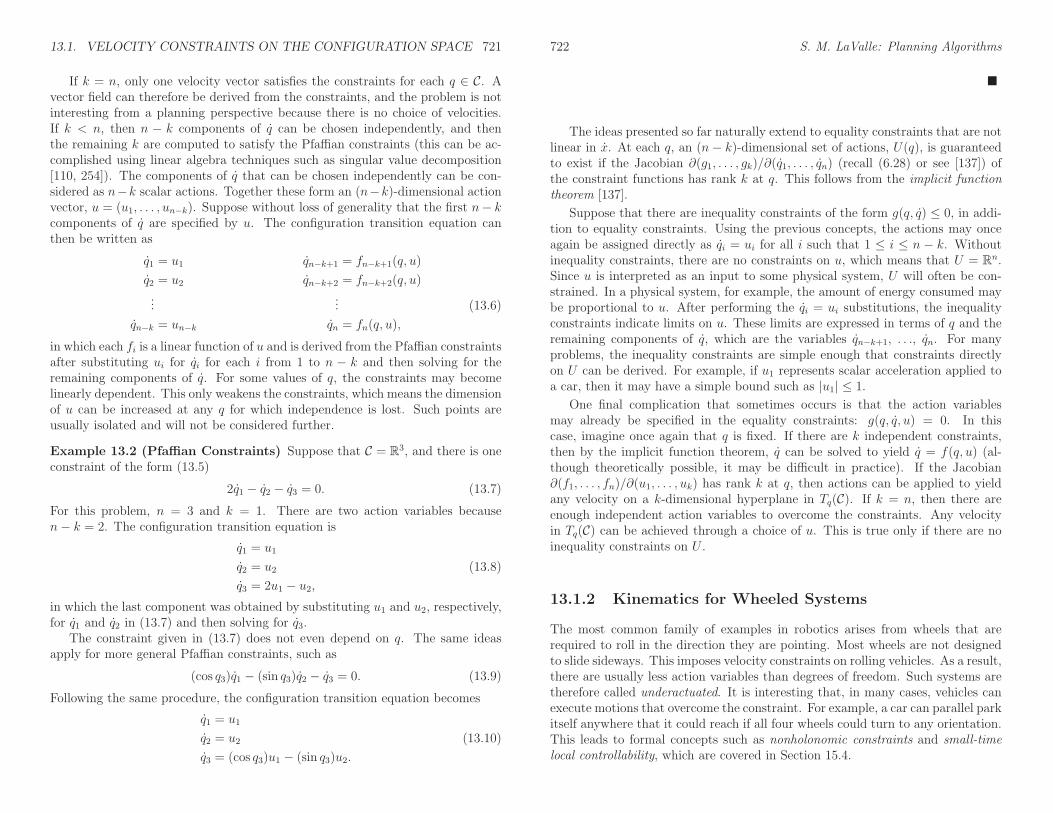
If k = n, only one velocity vector satisfies the constraints for each q ∈ C. Avector field can therefore be derived from the constraints, and the problem is notinteresting from a planning perspective because there is no choice of velocities.If k < n, then n − k components of q can be chosen independently, and thenthe remaining k are computed to satisfy the Pfaffian constraints (this can be ac-complished using linear algebra techniques such as singular value decomposition[110, 254]). The components of q that can be chosen independently can be con-sidered as n−k scalar actions. Together these form an (n−k)-dimensional actionvector, u = (u1, . . . , un−k). Suppose without loss of generality that the first n− kcomponents of q are specified by u. The configuration transition equation canthen be written as
q1 = u1 qn−k+1 = fn−k+1(q, u)
q2 = u2 qn−k+2 = fn−k+2(q, u)
...... (13.6)
qn−k = un−k qn = fn(q, u),
in which each fi is a linear function of u and is derived from the Pfaffian constraintsafter substituting ui for qi for each i from 1 to n − k and then solving for theremaining components of q. For some values of q, the constraints may becomelinearly dependent. This only weakens the constraints, which means the dimensionof u can be increased at any q for which independence is lost. Such points areusually isolated and will not be considered further.
Example 13.2 (Pfaffian Constraints) Suppose that C = R3, and there is one
constraint of the form (13.5)
2q1 − q2 − q3 = 0. (13.7)
For this problem, n = 3 and k = 1. There are two action variables becausen− k = 2. The configuration transition equation is
q1 = u1
q2 = u2
q3 = 2u1 − u2,(13.8)
in which the last component was obtained by substituting u1 and u2, respectively,for q1 and q2 in (13.7) and then solving for q3.
The constraint given in (13.7) does not even depend on q. The same ideasapply for more general Pfaffian constraints, such as
(cos q3)q1 − (sin q3)q2 − q3 = 0. (13.9)
Following the same procedure, the configuration transition equation becomes
q1 = u1
q2 = u2
q3 = (cos q3)u1 − (sin q3)u2.
(13.10)
722 S. M. LaValle: Planning Algorithms
�
The ideas presented so far naturally extend to equality constraints that are notlinear in x. At each q, an (n− k)-dimensional set of actions, U(q), is guaranteedto exist if the Jacobian ∂(g1, . . . , gk)/∂(q1, . . . , qn) (recall (6.28) or see [137]) ofthe constraint functions has rank k at q. This follows from the implicit functiontheorem [137].
Suppose that there are inequality constraints of the form g(q, q) ≤ 0, in addi-tion to equality constraints. Using the previous concepts, the actions may onceagain be assigned directly as qi = ui for all i such that 1 ≤ i ≤ n − k. Withoutinequality constraints, there are no constraints on u, which means that U = R
n.Since u is interpreted as an input to some physical system, U will often be con-strained. In a physical system, for example, the amount of energy consumed maybe proportional to u. After performing the qi = ui substitutions, the inequalityconstraints indicate limits on u. These limits are expressed in terms of q and theremaining components of q, which are the variables qn−k+1, . . ., qn. For manyproblems, the inequality constraints are simple enough that constraints directlyon U can be derived. For example, if u1 represents scalar acceleration applied toa car, then it may have a simple bound such as |u1| ≤ 1.
One final complication that sometimes occurs is that the action variablesmay already be specified in the equality constraints: g(q, q, u) = 0. In thiscase, imagine once again that q is fixed. If there are k independent constraints,then by the implicit function theorem, q can be solved to yield q = f(q, u) (al-though theoretically possible, it may be difficult in practice). If the Jacobian∂(f1, . . . , fn)/∂(u1, . . . , uk) has rank k at q, then actions can be applied to yieldany velocity on a k-dimensional hyperplane in Tq(C). If k = n, then there areenough independent action variables to overcome the constraints. Any velocityin Tq(C) can be achieved through a choice of u. This is true only if there are noinequality constraints on U .
13.1.2 Kinematics for Wheeled Systems
The most common family of examples in robotics arises from wheels that arerequired to roll in the direction they are pointing. Most wheels are not designedto slide sideways. This imposes velocity constraints on rolling vehicles. As a result,there are usually less action variables than degrees of freedom. Such systems aretherefore called underactuated. It is interesting that, in many cases, vehicles canexecute motions that overcome the constraint. For example, a car can parallel parkitself anywhere that it could reach if all four wheels could turn to any orientation.This leads to formal concepts such as nonholonomic constraints and small-timelocal controllability, which are covered in Section 15.4.

13.1. VELOCITY CONSTRAINTS ON THE CONFIGURATION SPACE 723
L
ρ
φ
θ
(x, y)
Figure 13.1: The simple car has three degrees of freedom, but the velocity spaceat any configuration is only two-dimensional.
A simple car
One of the easiest examples to understand is the simple car, which is shown inFigure 13.1. We all know that a car cannot drive sideways because the back wheelswould have to slide instead of roll. This is why parallel parking is challenging.If all four wheels could be turned simultaneously toward the curb, it would betrivial to park a car. The complicated maneuvers for parking a simple car arisebecause of rolling constraints.
The car can be imagined as a rigid body that moves in the plane. Therefore,its C-space is C = R
2 × S1. Figure 13.1 indicates several parameters associated
with the car. A configuration is denoted by q = (x, y, θ). The body frame of thecar places the origin at the center of rear axle, and the x-axis points along themain axis of the car. Let s denote the (signed) speed2 of the car. Let φ denotethe steering angle (it is negative for the wheel orientations shown in Figure 13.1).The distance between the front and rear axles is represented as L. If the steeringangle is fixed at φ, the car travels in a circular motion, in which the radius of thecircle is ρ. Note that ρ can be determined from the intersection of the two axesshown in Figure 13.1 (the angle between these axes is |φ|).
Using the current notation, the task is to represent the motion of the car as a
2Having a signed speed is somewhat unorthodox. If the car moves in reverse, then s isnegative. A more correct name for s would be velocity in the x direction of the body frame, butthis is too cumbersome.
724 S. M. LaValle: Planning Algorithms
set of equations of the form
x = f1(x, y, θ, s, φ)
y = f2(x, y, θ, s, φ)
θ = f3(x, y, θ, s, φ).
(13.11)
In a small time interval, ∆t, the car must move approximately in the directionthat the rear wheels are pointing. In the limit as ∆t tends to zero, this impliesthat dy/dx = tan θ. Since dy/dx = y/x and tan θ = sin θ/ cos θ, this conditioncan be written as a Pfaffian constraint (recall (13.5)):
−x sin θ + y cos θ = 0. (13.12)
The constraint is satisfied if x = cos θ and y = sin θ. Furthermore, any scalarmultiple of this solution is also a solution; the scaling factor corresponds directlyto the speed s of the car. Thus, the first two scalar components of the configurationtransition equation are x = s cos θ and y = s sin θ.
The next task is to derive the equation for θ. Let w denote the distancetraveled by the car (the integral of speed). As shown in Figure 13.1, ρ representsthe radius of a circle that is traversed by the center of the rear axle, if the steeringangle is fixed. Note that dw = ρdθ. From trigonometry, ρ = L/ tanφ, whichimplies
dθ =tanφ
Ldw. (13.13)
Dividing both sides by dt and using the fact that w = s yields
θ =s
Ltanφ. (13.14)
So far, the motion of the car has been modeled, but no action variables havebeen specified. Suppose that the speed s and steering angle φ are directly specifiedby the action variables us and uφ, respectively. The convention of using a uvariable with the old variable name appearing as a subscript will be followed.This makes it easy to identify the actions in a configuration transition equation.A two-dimensional action vector, u = (us, uφ), is obtained. The configurationtransition equation for the simple car is
x = us cos θ
y = us sin θ
θ =usL
tan uφ.
(13.15)
As expressed in (13.15), the transition equation is not yet complete withoutspecifying U , the set of actions of the form u = (us, uφ). First suppose that anyus ∈ R is possible. What steering angles are possible? The interval [−π/2, π/2]is sufficiently large for the steering angle uφ because any other value is equivalent

13.1. VELOCITY CONSTRAINTS ON THE CONFIGURATION SPACE 725
to one between −π/2 and π/2. Steering angles of π/2 and −π/2 are problematic.To derive the expressions for x and y, it was assumed that the car moves in thedirection that the rear wheels are pointing. Imagine you are sitting on a tricycleand turn the front wheel perpendicular to the rear wheels (assigning uφ = π/2).If you are able to pedal, then the tricycle should rotate in place. This means thatx = y = 0 because the center of the rear axle does not translate.
This strange behavior is not allowed for a standard automobile. A car withrear-wheel drive would probably skid the front wheels across the pavement. If acar with front-wheel drive attempted this, it should behave as a tricycle; however,this is usually not possible because the front wheels would collide with the frontaxle when turned to φ = π/2. Therefore, the simple car should have a maximumsteering angle, φmax < π/2, and we require that |φ| ≤ φmax. Observe from Figure13.1 that a maximum steering angle implies a minimum turning radius, ρmin. Forthe case of a tricycle, ρmin = 0. You may have encountered the problem of aminimum turning radius while trying to make an illegal U-turn. It is sometimesdifficult to turn a car around without driving it off of the road.
Now return to the speed us. On level pavement, a real vehicle has a topspeed, and its behavior should change dramatically depending on the speed. Forexample, if you want to drive along the minimum turning radius, you should notdrive at 140km/hr. It seems that the maximum steering angle should reduce athigher speeds. This enters the realm of dynamics, which will be allowed afterphase spaces are introduced in Section 13.2. Following this, some models of carswith dynamics will be covered in Sections 13.2.4 and 13.3.3.
It has been assumed implicitly that the simple car is moving slowly to safelyneglect dynamics. A bound such as |us| ≤ 1 can be placed on the speed withoutaffecting the configurations that it can reach. The speed can even be constrainedas us ∈ {−1, 0, 1} without destroying reachability. Be careful, however, about abound such as 0 ≤ us ≤ 1. In this case, the car cannot drive in reverse! Thisclearly affects the set of reachable configurations. Imagine a car that is facing awall and is unable to move in reverse. It may be forced to hit the wall as it moves.
Based on these considerations regarding the speed and steering angle, severalinteresting variations are possible:
Tricycle: U = [−1, 1]× [−π/2, π/2]. Assuming front-wheel drive, the “car”can rotate in place if uφ = π/2 or uφ = π/2. This is unrealistic for a simplecar. The resulting model is similar to that of the simple unicycle, whichappears later in (13.18).
Simple Car [164]: U = [−1, 1]× (−φmax, φmax). By requiring that |uφ| ≤φmax < π/2, a car with minimum turning radius ρmin = L/ tanφmax isobtained.
Reeds-Shepp Car [212, 245]: Further restrict the speed of the simple
726 S. M. LaValle: Planning Algorithms
car so that us ∈ {−1, 0, 1}.3 This model intuitively makes us correspond tothree discrete “gears”: reverse, park, or forward. An interesting questionunder this model is: What is the shortest possible path (traversed in R
2
by the center of the rear axle) between two configurations in the absence ofobstacles? This is answered in Section 15.3.
Dubins Car [85]: Remove the reverse speed us = −1 from the Reeds-Shepp car to obtain us ∈ {0, 1} as the only possible speeds. The shortestpaths in R
2 for this car are quite different than for the Reeds-Shepp car; seeSection 15.3.
The car that was shown in Figure 1.12a of Section 1.2 is even more restricted thanthe Dubins car because it is additionally forced to turn left.
Basic controllability issues have been studied thoroughly for the simple car.These will be covered in Section 15.4, but it is helpful to develop intuitive no-tions here to assist in understanding the planning algorithms of Chapter 14. Thesimple car is considered nonholonomic because there are differential constraintsthat cannot be completely integrated. This means that the car configurationsare not restricted to a lower dimensional subspace of C. The Reeds-Shepp carcan be maneuvered into an arbitrarily small parking space, provided that a smallamount of clearance exists. This property is called small-time local controllabilityand is presented in Section 15.1.3. The Dubins car is nonholonomic, but it doesnot possess this property. Imagine the difficulty of parallel parking without usingthe reverse gear. In an infinitely large parking lot without obstacles, however, theDubins car can reach any configuration.
A differential drive
Most indoor mobile robots do not move like a car. For example, consider themobile robotics platform shown in Figure 13.2a. This is an example of the mostpopular way to drive indoor mobile robots. There are two main wheels, each ofwhich is attached to its own motor. A third wheel (not visible in Figure 13.2a) isplaced in the rear to passively roll along while preventing the robot from fallingover.
To construct a simple model of the constraints that arise from the differentialdrive, only the distance L between the two wheels, and the wheel radius, r, arenecessary. See Figure 13.2b. The action vector u = (ur, ul) directly specifies thetwo angular wheel velocities (e.g., in radians per second). Consider how the robotmoves as different actions are applied. See Figure 13.3. If ul = ur > 0, then therobot moves forward in the direction that the wheels are pointing. The speed isproportional to r. In general, if ul = ur, then the distance traveled over a durationt of time is rtul (because tul is the total angular displacement of the wheels). If
3In many works, the speed us = 0 is not included. It appears here so that a proper terminationcondition can be defined.

13.1. VELOCITY CONSTRAINTS ON THE CONFIGURATION SPACE 727
r
L
x
y
(a) (b)
Figure 13.2: (a) The Pioneer 3-DX8 (courtesy of ActivMedia Robotics: MobileR-obots.com), and many other mobile robots use a differential drive. In addition tothe two drive wheels, a caster wheel (as on the bottom of an office chair) is placedin the rear center to prevent the robot from toppling over. (b) The parameters ofa generic differential-drive robot.
(a) (b)
Figure 13.3: (a) Pure translation occurs when both wheels move at the same angu-lar velocity; (b) pure rotation occurs when the wheels move at opposite velocities.
728 S. M. LaValle: Planning Algorithms
ul = −ur 6= 0, then the robot rotates clockwise because the wheels are turning inopposite directions. This motivates the placement of the body-frame origin at thecenter of the axle between the wheels. By this assignment, no translation occursif the wheels rotate at the same rate but in opposite directions.
Based on these observations, the configuration transition equation is
x =r
2(ul + ur) cos θ
y =r
2(ul + ur) sin θ
θ =r
L(ur − ul).
(13.16)
The translational part contains cos θ and sin θ parts, just like the simple car be-cause the differential drive moves in the direction that its drive wheels are pointing.The translation speed depends on the average of the angular wheel velocities. Tosee this, consider the case in which one wheel is fixed and the other rotates. Thisinitially causes the robot to translate at 1/2 of the speed in comparison to bothwheels rotating. The rotational speed θ is proportional to the change in angularwheel speeds. The robot’s rotation rate grows linearly with the wheel radius butreduces linearly with respect to the distance between the wheels.
It is sometimes preferable to transform the action space. Let uω = (ur + ul)/2and uψ = ur − ul. In this case, uω can be interpreted as an action variable thatmeans “translate,” and uψ means “rotate.” Using these actions, the configurationtransition equation becomes
x = ruω cos θ
y = ruω sin θ
θ =r
Luψ.
(13.17)
In this form, the configuration transition equation resembles (13.15) for the simplecar (try setting uψ = tan uφ and us = ruω). A differential drive can easily simulatethe motions of the simple car. For the differential drive, the rotation rate can beset independently of the translational velocity. The simple car, however, has thespeed us appearing in the θ expression. Therefore, the rotation rate depends onthe translational velocity.
Recall the question asked about shortest paths for the Reeds-Shepp and Du-bins cars. The same question for the differential drive turns out to be uninterestingbecause the differential drive can cause the center of its axle to follow any con-tinuous path in R
2. As depicted in Figure 13.4, it can move between any twoconfigurations by: 1) first rotating itself to point the wheels to the goal position,which causes no translation; 2) translating itself to the goal position; and 3) ro-tating itself to the desired orientation, which again causes no translation. Thetotal distance traveled by the center of the axle is always the Euclidean distancein R
2 between the two desired positions.

13.1. VELOCITY CONSTRAINTS ON THE CONFIGURATION SPACE 729
Figure 13.4: The shortest path traversed by the center of the axle is simply theline segment that connects the initial and goal positions in the plane. Rotationsappear to be cost-free.
θr
y
x
Figure 13.5: Viewed from above, the unicycle model has an action uω that changesthe wheel orientation θ.
This may seem like a strange effect due to the placement of the coordinateorigin. Rotations seem to have no cost. This can be fixed by optimizing thetotal amount of wheel rotation or time required, if the speed is held fixed [18].Suppose that ur, ul ∈ {−1, 0, 1}. Determining the minimum time required totravel between two configurations is quite interesting and is covered in Section15.3. This properly takes into account the cost of rotating the robot, even if itdoes not cause a translation.
A simple unicycle
Consider the simple model of a unicycle, which is shown in Figure 13.5. Ignoringbalancing concerns, there are two action variables. The rider of the unicycle canset the pedaling speed and the orientation of the wheel with respect to the z-axis.
730 S. M. LaValle: Planning Algorithms
d1 (x, y)
θ2
θ1
d2
θ0
Lφ
Figure 13.6: The parameters for a car pulling trailers.
Let σ denote the pedaling angular velocity, and let r be the wheel radius. Thespeed of the unicycle is s = rσ. In this model, the speed is set directly by anaction variable us (alternatively, the pedaling rate could be an action variable uσ,and the speed is derived as s = ruσ). Let ω be the angular velocity of the unicycleorientation in the xy plane (hence, ω = θ). Let ω be directly set by an actionvariable uω. The configuration transition equation is
x = us cos θ
y = us sin θ
θ = uω.
(13.18)
This is just the differential drive equation (13.17) with L = 1 and the substitutionus = ruσ. Thus, a differential drive can simulate a unicycle. This may seemstrange; however, it is possible because these models do not consider dynamics.Note that the unicycle can also simulate the simple-car model. Therefore, thetricycle and unicycle models are similar.
A car pulling trailers
An interesting extension of the simple car can be made by attaching one or moretrailers. You may have seen a train of luggage carts on the tarmac at airports.There are many subtle issues for modeling the constraints for these models. Theform of equations is very sensitive to the precise point at which the trailer isattached and also on the choice of body frames. One possibility for expressingthe kinematics is to use the expressions in Section 3.3; however, these may lead tocomplications when analyzing the constraints. It is somewhat of an art to find asimple expression of the constraints. The model given here is adapted from [194].4
4The original model required a continuous steering angle.

13.1. VELOCITY CONSTRAINTS ON THE CONFIGURATION SPACE 731
Consider a simple car that pulls k trailers as shown in Figure 13.6. Each traileris attached to the center of the rear axle of the body in front of it. The importantnew parameter is the hitch length di which is the distance from the center of therear axle of trailer i to the point at which the trailer is hitched to the next body.Using concepts from Section 3.3.1, the car itself contributes R
2 × S1 to C, and
each trailer contributes an S1 component to C. The dimension of C is therefore
k + 3. Let θi denote the orientation of the ith trailer, expressed with respect tothe world frame.
The configuration transition equation is
x = s cos θ0
y = s sin θ0
θ0 =s
Ltanφ
θ1 =s
d1sin(θ0 − θ1)
...
θi =s
di
(
i−1∏
j=1
cos(θj−1 − θj))
sin(θi−1 − θi)
...
θk =s
dk
(
k−1∏
j=1
cos(θj−1 − θj))
sin(θk−1 − θk).
(13.19)
An interesting variation of this model is to allow the trailer wheels to be steered.For a single trailer, this leads to a model that resembles a firetruck [54].
13.1.3 Other Examples of Velocity Constraints
The differential models seen so far were obtained from wheels that roll along aplanar surface. Many generalizations are possible by considering other ways inwhich bodies can contact each other. In robotics, many interesting differentialmodels arise in the context of manipulation. This section briefly covers someother examples of velocity constraints on the C-space. Once again, dynamics isneglected for now. Such models are sometimes classified as quasi-static becauseeven though motions occur, some aspects of the model treat the bodies as if theywere static. Such models are often realistic when moving at slow enough speeds.
Pushing a box
Imagine using a differential drive robot to push a box around on the floor, asshown in Figure 13.7a. It is assumed that the box is a convex polygon, one edgeof which contacts the front of the robot. There are frictional contacts between
732 S. M. LaValle: Planning Algorithms
Robot Box
(a) Stable pushing (b) Illegal sliding (c) Illegal rotation
Figure 13.7: Lynch and Mason showed that pushing a box is very much like drivingthe simple car: (a) With careful motions, the box will act as if it is attached tothe robot. b) If it turns too sharply, however, the box will slide away; this induceslimits on the steering angle. c) The box may alternatively rotate from sharp turns[178].
the box and floor and also between the box and robot. Suppose that the robot ismoving slowly enough so that dynamics are insignificant. It is assumed that thebox cannot move unless the robot is moving. This prohibits manipulations suchas “kicking” the box across the room. The term stable pushing [3, 178, 182] refersto the case in which the robot moves the box as if the box were rigidly attachedto the robot.
As the robot pushes the box, the box may slide or rotate, as shown in Figures13.7b and 13.7c, respectively. These cases are considered illegal because they donot constitute stable pushing. What motions of the robot are possible? Beginwith the configuration transition equation of the differential drive robot, and thendetermine which constraints need to be placed on U to maintain stable pushing.Suppose that (13.17) is used. It is clear that only forward motion is possiblebecause the robot immediately breaks contact with the box if the robot movesin the opposite direction. Thus, s must be positive (also, to fit the quasi-staticmodel, s should be small enough so that dynamical effects become insignificant).How should the rotation rate ψ be constrained? Constraints on ψ depend on thefriction model (e.g., Coulomb), the shape of the box, and the particular edge thatis being pushed. Details on these constraints are given in [178, 182]. This leadsto an interval [a, b] ⊆ [−π/2, π/2], in which a < 0 and b > 0, and it is requiredthat ψ ∈ [a, b]. This combination of constraints produces a motion model thatis similar to the Dubins car. The main difference is that the maximum steeringangle in the left and right directions may be different.
To apply this model for planning, it seems that the C-space should be R2×S1×R
2×S1 because there are two rigid bodies. The manipulation planning frameworkof Section 7.3.2 can be applied to obtain a hybrid system and manipulation graphthat expresses the various ways in which the robot can contact the box or fail tocontact the box. For example, the robot may be able to push the box along one

13.1. VELOCITY CONSTRAINTS ON THE CONFIGURATION SPACE 733
of several possible edges. If the robot becomes stuck, it can change the pushingedge to move the box in a new direction.
Flying an airplane
The Dubins car model from Section 13.1.2 can be extended to 3D worlds to providea simple aircraft flight model that may be reasonable for air traffic analysis. Firstsuppose that the aircraft maintains a fixed altitude and is capable only of yawrotations. In this case, (13.15) could be used directly by imposing the constraintthat s = 1 (or some suitable positive speed). This is equivalent to the Dubinscar, except that s = 0 is prohibited because it would imply that the aircraft caninstantaneously stop in the air. This model assumes that the aircraft is smallrelative to the C-space. A more precise model should take into account pitch androll rotations, disturbances, and dynamic effects. These would become important,for example, in studying the flight stability of an aircraft design. Such concernsare neglected here.
Now consider an aircraft that can change its altitude, in addition to executingmotions like the Dubins car. In this case let C = R
3 × S1, in which the extra R
represents the altitude with respect to flying over a flat surface. A configurationis represented as q = (x, y, z, θ). Let uz denote an action that directly causesa change in the altitude: z = uz. The steering action uφ is the same as in theDubins car model. The configuration transition equation is
x = cos θ z = uz
y = sin θ θ = uω. (13.20)
For a fixed value of u = (uz, uω) such that uz 6= 0 and uω 6= 0, a helical pathresults. The central axis of the helix is parallel to the z-axis, and projection of thepath down to the xy plane is a circle or circular arc. Maximum absolute valuesshould be set for uz and uω based on the maximum possible altitude and yaw ratechanges of the aircraft.
Rolling a ball
Instead of a wheel, consider rolling a ball in the plane. Place a ball on a tableand try rolling it with your palm placed flat on top of it. It should feel like thereare two degrees of freedom: rolling forward and rolling side to side. The ballshould not be able to spin in place. The directions can be considered as twoaction variables. The total degrees of freedom of the ball is five, however, becauseit can achieve any orientation in SO(3) and any (x, y) position in the plane; thus,C = R
2 × SO(3). Given that there are only two action variables, is it possible toroll the ball into any configuration? It is shown in [171, 133] that this is possible,even for the more general problem of one sphere rolling on another (the plane isa special case of a sphere with infinite radius). This problem can actually arise
734 S. M. LaValle: Planning Algorithms
in robotic manipulation when a spherical object come into contact (e.g., a robothand may have fingers with spherical tips); see [32, 180, 192, 195].
The resulting transition equation was shown in [189] (also see [192]) to be
θ = −u2φ =
u1cos θ
x = −u1ρ sinψ − u2ρ cosψy = −u1ρ cosψ + u2ρ sinψ
ψ = −u1 tan θ.
(13.21)
In these equations, x and y are the position on the contact point in the plane, andθ and φ are the position of the contact point in the ball frame and are expressedusing spherical coordinates. The radius of the ball is ρ. Finally, ψ expresses theorientation of the ball with respect to the contact point.
Trapped on a surface
It is possible that the constraints cause the configuration to be trapped on a lowerdimensional surface. Let C = R
2, and consider the system
x = yu y = −xu, (13.22)
for (x, y) ∈ R2 and u ∈ U = R. What are the integral curves for a constant
action u 6= 0? From any point (x, y) ∈ R2, the trajectory follows a circle of radius
√
x2 + y2 centered at the origin. The speed along the circle is determined by |u|,and the direction is determined by the sign of u. Therefore, (13.22) indicates thatthe configuration is confined to a circle. Other than that, there are no furtherconstraints.
Suppose that the initial configuration is given as (x0, y0). Since the configura-tion is confined to a circle, the C-space could alternatively be defined as C = S
1.Each point on S
1 can be mapped to the circle that has radius r =√
x20 + y20and center at (0, 0). In this case, there are no differential constraints on the ve-locities, provided that motions are trapped on the circle. Any velocity in theone-dimensional tangent space at points on the circle is allowed. This model isequivalent to (13.22).
Now consider the possible trajectories that are constrained to traverse a circle,
h(x, y) = x2 + y2 − r2 = 0. (13.23)
This means that for all time t,
h(x(t), y(t)) = x(t)2 + y(t)2 − r2 = 0. (13.24)
To derive a constraint on velocities, take the derivative with respect to time, whichyields
dh(x, y)
dt= 2xx+ 2yy = 0. (13.25)

13.2. PHASE SPACE REPRESENTATION OF DYNAMICAL SYSTEMS 735
This is an example of a Pfaffian constraint, as given in (13.5). The parametricform of this differential constraint happens to be (13.22). Any velocity vectorthat is a multiple of (y,−x) satisfies (13.25). When expressed as a differentialconstraint, the radius r does not matter. This is because it is determined fromthe initial configuration.
What just occurred here is a special case of a completely integrable differentialmodel. In general, if the model q = f(q, u) can be expressed as the time derivativeof constraints of the form h(q) = 0, then the configuration transition equation issaid to be completely integrable. Obtaining an implicit differential model fromconstraints of the form hi(q) = 0 is not difficult. Each constraint is differentiatedto obtain
dhi(q)
dt= 0. (13.26)
For example, such constraints arise from closed kinematic chains, as in Section4.4, and the implicit differential model just expresses the condition that velocitiesmust lie in the tangent space to the constraints. It may be difficult, however, toobtain a parametric form of the differential model. Possible velocity vectors canbe computed at any particular q, however, by using the linear algebra techniquesdescribed in Section 7.4.1.
It is even quite difficult to determine whether a differential model is completelyintegrable, which means that the configurations are trapped on a lower dimen-sional surface. For some systems, to be described by (13.41), this will be solved bythe Frobenius Theorem in 15.4.2. If such systems are not completely integrable,they are called nonholonomic; otherwise, they are called holonomic. In general,even if a model is theoretically integrable, actually performing the integration isanother issue. In most cases, it is difficult or impossible to integrate the model.
Therefore, it is sometimes important to work directly with constraints in dif-ferential form, even if they are integrable. Furthermore, methods for planningunder differential constraints can be applied to problems that have constraints ofthe form h(q) = 0. This, for example, implies that motion planning for closedkinematic chains can be performed by planning algorithms designed to handledifferential constraints.
13.2 Phase Space Representation of Dynamical
Systems
The differential constraints defined in Section 13.1 are often called kinematic be-cause they can be expressed in terms of velocities on the C-space. This formulationis useful for many problems, such as modeling the possible directions of motionsfor a wheeled mobile robot. It does not, however, enable dynamics to be ex-pressed. For example, suppose that the simple car is traveling quickly. Takingdynamics into account, it should not be able to instantaneously start and stop.
736 S. M. LaValle: Planning Algorithms
For example, if it is heading straight for a wall at full speed, any reasonable modelshould not allow it to apply its brakes from only one millimeter away and expectit to avoid collision. Due to momentum, the required stopping distance dependson the speed. You may have learned this from a drivers education course.
To account for momentum and other aspects of dynamics, higher order dif-ferential equations are needed. There are usually constraints on acceleration q,which is defined as dq/dt. For example, the car may only be able to decelerateat some maximum rate without skidding the wheels (or tumbling the vehicle).Most often, the actions are even expressed in terms of higher order derivatives.For example, the floor pedal of a car may directly set the acceleration. It may bereasonable to consider the amount that the pedal is pressed as an action variable.In this case, the configuration must be obtained by two integrations. The firstyields the velocity, and the second yields the configuration.
The models for dynamics therefore involve acceleration q in addition to velocityq and configuration q. Once again, both implicit and parametric models exist. Foran implicit model, the constraints are expressed as
gi(q, q, q) = 0. (13.27)
For a parametric model, they are expressed as
q = f(q, q, u). (13.28)
13.2.1 Reducing Degree by Increasing Dimension
Taking into account constraints on higher order derivatives seems substantiallymore complicated. This section explains a convenient trick that converts con-straints that have higher order derivatives into a new set of constraints that hasonly first-order derivatives. This involves the introduction of a phase space, whichhas more dimensions than the original C-space. Thus, there is a trade-off becausethe dimension is increased; however, it is widely accepted that increasing the di-mension of the space is often easier than dealing with higher order derivatives. Ingeneral, the term state space will refer to either C-spaces or phase spaces derivedfrom them.
The scalar case
To make the discussion concrete, consider the following differential equation:
y − 3y + y = 0, (13.29)
in which y is a scalar variable, y ∈ R. This is a second-order differential equationbecause of y. A phase space can be defined as follows. Let x = (x1, x2) denote atwo-dimensional phase vector, which is defined by assigning x1 = y and x2 = y.The terms state space and state vector will be used interchangeably with phase

13.2. PHASE SPACE REPRESENTATION OF DYNAMICAL SYSTEMS 737
space and phase vector, respectively, in contexts in which the phase space isdefined. Substituting the equations into (13.29) yields
y − 3x2 + x1 = 0. (13.30)
So far, this does not seem to have helped. However, y can be expressed as eitherx2 or x1. The first choice is better because it is a lower order derivative. Usingx2 = y, the differential equation becomes
x2 − 3x2 + x1 = 0. (13.31)
Is this expression equivalent to (13.29)? By itself it is not. There is one moreconstraint, x2 = x1. In implicit form, x1 − x2 = 0. The key to making thephase space approach work correctly is to relate some of the phase variables byderivatives.
Using the phase space, we just converted the second-order differential equation(13.29) into two first-order differential equations,
x1 = x2
x2 = 3x2 − x1,(13.32)
which are obtained by solving for x1 and x2. Note that (13.32) can be expressedas x = f(x), in which f is a function that maps from R
2 into R2.
The same approach can be used for any differential equation in implicit form,g(y, y, y) = 0. Let x1 = y, x2 = y, and x2 = y. This results in the implicitequations g(x2, x2, x1) = 0 and x1 = x2. Now suppose that there is a scalaraction u ∈ U = R represented in the differential equations. Once again, thesame approach applies. In implicit form, g(y, y, y, u) = 0 can be expressed asg(x2, x2, x1, u) = 0.
Suppose that a given acceleration constraint is expressed in parametric formas y = h(y, y, u). This often occurs in the dynamics models of Section 13.3. Thiscan be converted into a phase transition equation or state transition equation ofthe form x = f(x, u), in which f : R2 × R→ R
2. The expression is
x1 = x2
x2 = h(x2, x1, u).(13.33)
For a second-order differential equation, two initial conditions are usuallygiven. The values of y(0) and y(0) are needed to determine the exact position y(t)for any t ≥ 0. Using the phase space representation, no higher order initial condi-tions are needed because any point in phase space indicates both y and y. Thus,given an initial point in the phase and u(t) for all t ≥ 0, y(t) can be determined.
Example 13.3 (Double Integrator) The double integrator is a simple yet im-portant example that nicely illustrates the phase space. Suppose that a second-order differential equation is given as q = u, in which q and u are chosen from R.
738 S. M. LaValle: Planning Algorithms
In words, this means that the action directly specifies acceleration. Integrating5
once yields the velocity q and performing a double integration yields the positionq. If q(0) and q(0) are given, and u(t′) is specified for all t′ ∈ [0, t), then q(t) andq(t) can be determined for any t > 0.
A two-dimensional phase space X = R2 is defined in which
x = (x1, x2) = (q, q). (13.34)
The state (or phase) transition equation x = f(x, u) is
x1 = x2
x2 = u.(13.35)
To determine the state trajectory, initial values x1(0) = q0 (position) and x2(0) =q0 (velocity) must be given in addition to the action history. If u is constant, thenthe state trajectory is quadratic because it is obtained by two integrations of aconstant function. �
The vector case
The transformation to the phase space can be extended to differential equationsin which there are time derivatives in more than one variable. Suppose that qrepresents a configuration, expressed using a coordinate neighborhood on a smoothn-dimensional manifold C. Second-order constraints of the form g(q, q, q) = 0 org(q, q, q, u) = 0 can be expressed as first-order constraints in a 2n-dimensionalstate space. Let x denote the 2n-dimensional phase vector. By extending themethod that was applied to the scalar case, x is defined as x = (q, q). For eachinteger i such that 1 ≤ i ≤ n, xi = qi. For each i such that n + 1 ≤ i ≤ 2n,xi = qi−n. These substitutions can be made directly into an implicit constraint toreduce the order to one.
Suppose that a set of n differential equations is expressed in parametric form asq = h(q, q, u). In the phase space, there are 2n differential equations. The first ncorrespond to the phase space definition xi = xn+i, for each i such that 1 ≤ i ≤ n.These hold because xn+i = qi and xi is the time derivative of qi for i ≤ n. Theremaining n components of x = f(x, u) follow directly from h by substituting thefirst n components of x in the place of q and the remaining n in the place of q inthe expression h(q, q, u). The result can be denoted as h(x, u) (obtained directlyfrom h(q, q, u)). This yields the final n equations as xi = hi−n(x, u), for each isuch that n+1 ≤ i ≤ 2n. These 2n equations define a phase (or state) transitionequation of the form x = f(x, u). Now it is clear that constraints on accelerationcan be manipulated into velocity constraints on the phase space. This enablesthe tangent space concepts from Section 8.3 to express constraints that involve
5Wherever integrals are performed, it will be assumed that the integrands are integrable.

13.2. PHASE SPACE REPRESENTATION OF DYNAMICAL SYSTEMS 739
acceleration. Furthermore, the state space X is the tangent bundle (defined in(8.9) for Rn and later in (15.67) for any smooth manifold) of C because q and qtogether indicate a tangent space Tq(C) and a particular tangent vector q ∈ Tq(C).
Higher order differential constraints
The phase space idea can even be applied to differential equations with orderhigher than two. For example, a constraint may involve the time derivativeof acceleration q(3), which is often called jerk. If the differential equations in-volve jerk variables, then a 3n-dimensional phase space can be defined to ob-tain first-order constraints. In this case, each qi, qi, and qi in a constraint suchas g(q(3), q, q, q, u) = 0 is defined as a phase variable. Similarly, kth-order dif-ferential constraints can be reduced to first-order constraints by introducing akn-dimensional phase space.
Example 13.4 (Chain of Integrators) A simple example of higher order dif-ferential constraints is the chain of integrators.6 This is a higher order general-ization of Example 13.3. Suppose that a kth-order differential equation is givenas q(k) = u, in which q and u are scalars, and q(k) denotes the kth derivative of qwith respect to time.
A k-dimensional phase space X is defined in which
x = (q, q, q, q(3), . . . , q(k−1)). (13.36)
The state (or phase) transition equation x = f(x, u) is xi = xi+1 for each i suchthat 1 ≤ i ≤ n − 1, and xn = u. Together, these n individual equations areequivalent to q(k) = u.
The initial state specifies the initial position and all time derivatives up toorder k − 1. Using these and the action u, the state trajectory can be obtainedby a chain of integrations. �
You might be wondering whether derivatives can be eliminated completely byintroducing a phase space that has high enough dimension. This does actuallywork. For example, if there are second-order constraints, then a 3n-dimensionalphase space can be introduced in which x = (q, q, q). This enables constraints suchas g(q, q, q) = 0 to appear as g(x) = 0. The trouble with using such formulationsis that the state must follow the constraint surface in a way that is similar totraversing the solution set of a closed kinematic chain, as considered in Section4.4. This is why tangent spaces arose in that context. In either case, the set ofallowable velocities becomes constrained at every point in the space.
Problems defined using phase spaces typically have an interesting propertyknown as drift. This means that for some x ∈ X, there does not exist any u ∈ U
6It is called this because in block diagram representations of systems it is depicted as a chainof integrator blocks.
740 S. M. LaValle: Planning Algorithms
such that f(x, u) = 0. For the examples in Section 13.1.2, such an action alwaysexisted. These were examples of driftless systems. This was possible because theconstraints did not involve dynamics. In a dynamical system, it is impossible toinstantaneously stop due to momentum, which is a form of drift. For example,a car will “drift” into a brick wall if it is 3 meters way and traveling 100 km/hrin the direction of the wall. There exists no action (e.g., stepping firmly on thebrakes) that could instantaneously stop the car. In general, there is no way toinstantaneously stop in the phase space.
13.2.2 Linear Systems
Now that the phase space has been defined as a special kind of state space thatcan handle dynamics, it is convenient to classify the kinds of differential modelsthat can be defined based on their mathematical form. The class of linear systemshas been most widely studied, particularly in the context of control theory. Thereason is that many powerful techniques from linear algebra can be applied toyield good control laws [58]. The ideas can also be generalized to linear systemsthat involve optimality criteria [5, 150], nature [27, 147], or multiple players [16].
Let X = Rn be a phase space, and let U = R
m be an action space for m ≤ n.A linear system is a differential model for which the state transition equation canbe expressed as
x = f(x, u) = Ax+ Bu, (13.37)
in which A and B are constant, real-valued matrices of dimensions n × n andn×m, respectively.
Example 13.5 (Linear System Example) For a simple example of (13.37),suppose X = R
3, U = R2, and let
x1x2x3
=
0√2 1
1 −1 42 0 1
x1x2x3
+
1 00 11 1
(
u1u2
)
. (13.38)
Performing the matrix multiplications reveals that all three equations are linear inthe state and action variables. Compare this to the discrete-time linear Gaussiansystem shown in Example 11.25. �
Recall from Section 13.1.1 that k linear constraints restrict the velocity to an(n − k)-dimensional hyperplane. The linear model in (13.37) is in parametricform, which means that each action variable may allow an independent degree offreedom. In this case, m = n − k. In the extreme case of m = 0, there are noactions, which results in x = Ax. The phase velocity x is fixed for every pointx ∈ X. If m = 1, then at every x ∈ X a one-dimensional set of velocities maybe chosen using u. This implies that the direction is fixed, but the magnitude is

13.2. PHASE SPACE REPRESENTATION OF DYNAMICAL SYSTEMS 741
chosen using u. In general, the set of allowable velocities at a point x ∈ Rn is an
m-dimensional linear subspace of the tangent space Tx(Rn) (if B is nonsingular).
In spite of (13.37), it may still be possible to reach all of the state space fromany initial state. It may be costly, however, to reach a nearby point because of therestriction on the tangent space; it is impossible to command a velocity in somedirections. For the case of nonlinear systems, it is sometimes possible to quicklyreach any point in a small neighborhood of a state, while remaining in a smallregion around the state. Such issues fall under the general topic of controllability,which will be covered in Sections 15.1.3 and 15.4.3.
Although not covered here, the observability of the system is an importanttopic in control [58, 130]. In terms of the I-space concepts of Chapter 11, thismeans that a sensor of the form y = h(x) is defined, and the task is to determinethe current state, given the history I-state. If the system is observable, this meansthat the nondeterministic I-state is a single point. Otherwise, the system mayonly be partially observable. In the case of linear systems, if the sensing model isalso linear,
y = h(x) = Cy, (13.39)
then simple matrix conditions can be used to determine whether the system isobservable [58]. Nonlinear observability theory also exists [130].
As in the case of discrete planning problems, it is possible to define differentialmodels that depend on time. In the discrete case, this involves a dependency onstages. For the continuous-stage case, a time-varying linear system is defined as
x = f(x(t), u(t), t) = A(t)x(t) + B(t)u(t). (13.40)
In this case, the matrix entries are allowed to be functions of time. Many powerfulcontrol techniques can be easily adapted to this case, but it will not be consideredhere because most planning problems are time-invariant (or stationary).
13.2.3 Nonlinear Systems
Although many powerful control laws can be developed for linear systems, thevast majority of systems that occur in the physical world fail to be linear. Anydifferential models that do not fit (13.37) or (13.40) are called nonlinear systems.All of the models given in Section 13.1.2 are nonlinear systems for the special casein which X = C.
One important family of nonlinear systems actually appears to be linear insome sense. Let X be a smooth n-dimensional manifold, and let U ⊆ R
m. LetU = R
m for some m ≤ n. Using a coordinate neighborhood, a nonlinear systemof the form
x = f(x) +m∑
i=1
gi(x)ui (13.41)
742 S. M. LaValle: Planning Algorithms
for smooth functions f and gi is called a control-affine system or affine-in-controlsystem.7 These have been studied extensively in nonlinear control theory [130,221]. They are linear in the actions but nonlinear with respect to the state. SeeSection 15.4.1 for further reading on control-affine systems.
For a control-affine system it is not necessarily possible to obtain zero velocitybecause f causes drift. The important special case of a driftless control-affinesystem occurs if f ≡ 0. This is written as
x =m∑
i=1
gi(x)ui. (13.42)
By setting ui = 0 for each i from 1 to m, zero velocity, x = 0, is obtained.
Example 13.6 (Nonholonomic Integrator) One of the simplest examples ofa driftless control-affine system is the nonholonomic integrator introduced in con-trol literature by Brockett in [46]. It some times referred to as Brockett’s sys-tem, or the Heisenberg system because it arises in quantum mechanics [34]. LetX = R
3, and let the set of actions U = R2. The state transition equation for the
nonholonomic integrator is
x1 = u1
x2 = u2
x3 = x1u2 − x2u1.(13.43)
�
Many nonlinear systems can be expressed implicitly using Pfaffian constraints,which appeared in Section 13.1.1, and can be generalized from C-spaces to phasespaces. In terms of X, a Pfaffian constraint is expressed as
g1(x)x1 + g2(x)x2 + · · ·+ gn(x)xn = 0. (13.44)
Even though the equation is linear in x, a nonlinear dependency on x is allowed.Both holonomic and nonholonomic models may exist for phase spaces, just
as in the case of C-spaces in Section 13.1.3. The Frobenius Theorem, which iscovered in Section 15.4.2, can be used to determine whether control-affine systemsare completely integrable.
13.2.4 Extending Models by Adding Integrators
The differential models from Section 13.1 may seem unrealistic in many applica-tions because actions are required to undergo instantaneous changes. For example,
7Be careful not to confuse control-affine systems with affine control systems, which are of theform x = Ax+Bu+ w, for some constant matrices A,B and a constant vector w.

13.2. PHASE SPACE REPRESENTATION OF DYNAMICAL SYSTEMS 743
in the simple car, the steering angle and speed may be instantaneously changedto any value. This implies that the car is capable of instantaneous accelerationchanges. This may be a reasonable approximation if the car is moving slowly(for example, to analyze parallel-parking maneuvers). The model is ridiculous,however, at high speeds.
Suppose a state transition equation of the form x = f(x, u) is given in whichthe dimension of X is n. The model can be enhanced as follows:
1. Select an action variable ui.
2. Rename the action variable as a new state variable, xn+1 = ui.
3. Define a new action variable u′i that takes the place of ui.
4. Extend the state transition equation by one dimension by introducing xn+1 =u′i.
This enhancement will be referred to as placing an integrator in front of ui. Thisprocedure can be applied incrementally as many times as desired, to create a chainof integrators from any action variable. It can also be applied to different actionvariables.
Better unicycle models
Improvements to the models in Section 13.1 can be made by placing integratorsin front of action variables. For example, consider the unicycle model (13.18).Instead of directly setting the speed using us, suppose that the speed is obtainedby integration of an action ua that represents acceleration. The equation s = uais used instead of s = us, which means that the action sets the change in speed. Ifua is chosen from some bounded interval, then the speed is a continuous functionof time.
How should the transition equation be represented in this case? The set ofpossible values for ua imposes a second-order constraint on x and y because doubleintegration is needed to determine their values. By applying the phase space idea,s can be considered as a phase variable. This results in a four-dimensional phasespace, in which each state is (x, y, θ, s). The state (or phase) transition equationis
x = s cos θ θ = uω
y = s sin θ s = ua, (13.45)
which should be compared to (13.18). The action us was replaced by s becausenow speed is a phase variable, and an extra equation was added to reflect theconnection between speed and acceleration.
The integrator idea can be applied again to make the unicycle orientations acontinuous function of time. Let uα denote an angular acceleration action. Let
744 S. M. LaValle: Planning Algorithms
ω denote the angular velocity, which is introduced as a new state variable. Thisresults in a five-dimensional phase space and a model called the second-orderunicycle:
x = s cos θ s = ua
y = s sin θ ω = uα (13.46)
θ = ω,
in which u = (ua, uα) is a two-dimensional action vector. In some contexts, s maybe fixed at a constant value, which implies that ua is fixed to ua = 0.
A continuous-steering car
As another example, consider the simple car. As formulated in (13.15), the steer-ing angle is allowed to change discontinuously. For simplicity, suppose that thespeed is fixed at s = 1. To make the steering angle vary continuously over time,let uω be an action that represents the velocity of the steering angle: φ = uω.The result is a four-dimensional state space, in which each state is represented as(x, y, θ, φ). This yields a continuous-steering car,
x = cos θ θ =tanφ
L
y = sin θ φ = uω, (13.47)
in which there are two action variables, us and uω. This model was used forplanning in [223].
A second integrator can be applied to make the steering angle a C1 smoothfunction of time. Let ω be a state variable, and let uα denote the angular acceler-ation of the steering angle. In this case, the state vector is (x, y, θ, φ, ω), and thestate transition equation is
x = cos θ φ = ω
y = sin θ ω = uα (13.48)
θ =tanφ
L.
Integrators can be applied any number of times to make any variables as smoothas desired. Furthermore, the rate of change in each case can be bounded due tolimits on the phase variables and on the action set.
Smooth differential drive
A second-order differential drive model can be made by defining actions ul and urthat accelerate the motors, instead of directly setting their velocities. Let ωl and

13.3. BASIC NEWTON-EULER MECHANICS 745
ωr denote the left and right motor angular velocities, respectively. The resultingstate transition equation is
x =r
2(ωl + ωr) cos θ ωl = ul
y =r
2(ωl + ωr) sin θ ωr = ur (13.49)
θ =r
L(ωr − ωl).
In summary, an important technique for making existing models somewhatmore realistic is to insert one or more integrators in front of any action variables.The dimension of the phase space increases with the introduction of each inte-grator. A single integrator forces an original action to become continuous overtime. If the new action is bounded, then the rate of change of the original ac-tion is bounded in places where it is differentiable (it is Lipschitz in general, asexpressed in (8.16)). Using a double integrator, the original action is forced to beC1 smooth. Chaining more integrators on an action variable further constrainsits values. In general, k integrators can be chained in front of an original actionto force it to be Ck−1 smooth and respect Lipschitz bounds.
One important limitation, however, is that to make realistic models, othervariables may depend on the new phase variables. For example, if the simple caris traveling fast, then we should not be able to turn as sharply as in the case of aslow-moving car (think about how sharply you can turn the wheel while parallelparking in comparison to driving on the highway). The development of betterdifferential models ultimately requires careful consideration of mechanics. Thisprovides motivation for Sections 13.3 and 13.4.
13.3 Basic Newton-Euler Mechanics
Mechanics is a vast and difficult subject. It is virtually impossible to providea thorough introduction in a couple of sections. Here, the purpose instead is tooverview some of the main concepts and to provide some models that may be usedwith the planning algorithms in Chapter 14. The presentation in this section andin Section 13.4 should hopefully stimulate some further studies in mechanics (seethe suggested literature at the end of the chapter). On the other hand, if youare only interested in using the differential models, then you can safely skip theirderivations. Just keep in mind that all differential models produced in this sectionend with the form x = f(x, u), which is ready to use in planning algorithms.
There are two important points to keep in mind while studying mechanics:
1. The models are based on maintaining consistency with experimental obser-vations about how bodies behave in the physical world. These observationsdepend on the kind of experiment. In a particular application, many effectsmay be insignificant or might not even be detectable by an experiment. For
746 S. M. LaValle: Planning Algorithms
example, it is difficult to detect relativistic effects using a radar gun thatmeasures automobile speed. It is therefore important to specify any simpli-fying assumptions regarding the world and the kind of experiments that willbe performed in it.
2. The approach is usually to express some laws that translate into constraintson the allowable velocities in the phase space. This means that implicitrepresentations are usually obtained in mechanics, and they must be con-verted into parametric form. Furthermore, most treatments of mechanicsdo not explicitly mention action variables; these arise from the intentionof controlling the physical world. From the perspective of mechanics, theactions can be assumed to be already determined. Thus, constraints appearas g(x, x) = 0, instead of g(x, x, u) = 0.
Several formulations of mechanics arrive at the same differential constraints,but from different mathematical reasoning. The remainder of this chapter overviewsthree schools of thought, each of which is more elegant and modern than theone before. The easiest to understand is Newton-Euler mechanics, which followsfrom Newton’s famous laws of physics and is covered in this section. Lagrangianmechanics is covered in Section 13.4.1 and arrives at the differential constraintsusing very general principles of optimization on a space of functions (i.e., calculusof variations). Hamiltonian mechanics, covered in Section 13.4.4, defines a higherdimensional state space on which the differential constraints can once again beobtained by optimization.
13.3.1 The Newtonian Model
The most basic formulation of mechanics goes back to Newton and Euler, andparts of it are commonly studied in basic physics courses. Consider a world Wdefined as in Section 3.1, except here a 1D world W = R is allowed, in additionto 2D and 3D worlds. A notion of time is also needed. The space of motionsthat can be obtained in the space-time continuum can be formalized as a Galileangroup [10]; however, the presentation here will utilize standard intuitive notionsof time and Euclidean space. It is also assumed that any relativistic effects due tocurvature of the time-space continuum are nonexistent (Newton and Euler did notknow about this, and it is insignificant for most small-scale mechanical systemson or near the earth).
Inertial coordinate frames Central to Newton-Euler mechanics is the ideathat points in W are expressed using an inertial coordinate frame. Imagine locat-ing the origin and axes ofW somewhere in our universe. They need to be fixed ina way that does not interfere with our observations of the basic laws of motion.Imagine that we are playing racquetball in an indoor court and want to modelthe motion of the ball as it bounces from wall to wall. If the coordinate frame is

13.3. BASIC NEWTON-EULER MECHANICS 747
rigidly attached to the ball, it will appear that the ball never moves; however, thewalls, earth, and the rest of the universe will appear to spin wildly around theball (imagine we have camera that points along some axis of the ball frame – youcould quickly become ill trying to follow the movie). If the coordinate frame isfixed with respect to the court, then sensible measurements of the ball positionswould result (the movie would also be easier to watch). For all practical purposes,we can consider this fixed coordinate frame to be inertial. Note, however, that theball will dance around wildly if the coordinate frame is instead fixed with respectto the sun. The rotation and revolution of the earth would cause the ball to moveat incredible speeds. In reality, inertial frames do not exist; nevertheless, it is areasonable assumption for earth-based mechanical systems that an inertial framemay be fixed to the earth.
The properties that inertial frames should technically possess are 1) the lawsof motions appear the same in any inertial frame, and 2) any frame that moves atconstant speed without rotation with respect to an inertial frame is itself inertial.As an example of the second condition, suppose that the racquetball experimentis performed inside of a big truck that is driving along a highway. Ignoring vibra-tions, if the truck moves at constant speed on a straight stretch of road, then aninertial coordinate frame can be fixed to the truck itself, and the ball will appearto bounce as if the court was not moving. If, however, the road curves or the truckchanges its speed, the ball will not bounce the right way. If we still believe thatthe frame attached to the truck is inertial, then the laws of motion will appearstrange. The inertial frame must be attached to the earth in this case to correctlymodel the behavior of the truck and ball together.
Closed system Another important aspect of the Newton-Euler model is thatthe system of bodies for which motions are modeled is closed, which means thatno bodies other than those that are explicitly modeled can have any affect on themotions (imagine, for example, the effect if we forget to account for a black holethat is a few hundred meters away from the racquetball court).
Newton’s laws The motions of bodies are based on three laws that were ex-perimentally verified by Newton and should hold in any inertial frame:
1. An object at rest tends to stay at rest, and an object in motion tends tostay in motion with fixed speed, unless a nonzero resultant8 force acts uponit.
2. The relationship between a body mass m, its acceleration a, and an appliedforce f is f = ma.
3. The interaction forces between two bodies are of equal magnitude and inopposite directions.
8This is the sum of all forces acting on the point.
748 S. M. LaValle: Planning Algorithms
Based on these laws, the differential constraints on a system of moving bodies canbe modeled.
13.3.2 Motions of Particles
The Newton-Euler model is described in terms of particles. Each particle is con-sidered as a point that has an associated mass m. Forces may act on any particle.The motion of a rigid body, covered in Section 13.3.3, is actually determined bymodeling the body as a collection of particles that are stuck together. Therefore,it is helpful to first understand how particles behave.
Motion of a single particle
Consider the case of a single particle of mass m that moves in W = R. The forcebecomes a scalar, f ∈ R. Let q(t) denote the position of the particle in W attime t. Using this notation, acceleration is q, and Newton’s second law becomesf = mq. This can be solved for q to yield
q = f/m. (13.50)
If f is interpreted as an action variable u, and if m = 1, then (13.50) is preciselythe double integrator q = u from Example 13.3. Phase variables x1 = q andx2 = q can be introduced to obtain a state vector x = (q, q). This means that fora fixed u, the motion of the particle from any initial state can be captured by avector field on R
2. The state transition equation is
x1 = x2
x2 =u
m,
(13.51)
in which x1 = q, x2 = q, and u = f . Let U = [−fmax, fmax], in which fmax repre-sents the maximum magnitude of force that can be applied to the particle. Forcesof arbitrarily high magnitude are not allowed because this would be physicallyunrealistic.
Now generalize the particle motion to W = R2 and W = R
3. Let n denotethe dimension of W , which may be n = 2 or n = 3. Let q denote the positionof the particle in W . Once again, Newton’s second law yields f = mq, but inthis case there are n independent equations of the form fi = mqi. Each of thesemay be considered as an independent example of the double integrator, scaled bym. Each component fi of the force can be considered as an action variable ui.A 2n-dimensional state space can be defined as x = (q, q). The state transitionequation for n = 2 becomes
x1 = x3 x3 = u1/m (13.52)
x2 = x4 x4 = u2/m,

13.3. BASIC NEWTON-EULER MECHANICS 749
mg
fu
flfr
Figure 13.8: There are three thrusters on the lunar lander, and it is under theinfluence of lunar gravity. It is treated as a particle; therefore, no rotations arepossible. Four orthogonal forces may act on the lander: Three arise from thrustersthat can be switched on or off, and the remaining arises from the acceleration ofgravity.
and for n = 3 it becomes
x1 = x4 x4 = u1/m
x2 = x5 x5 = u2/m (13.53)
x3 = x6 x6 = u3/m.
For a fixed action, these equations define vector fields on R4 and R
6, respectively.The action set should also be bounded, as in the one-dimensional case. Supposethat
U = {u ∈ Rn | ‖u‖ ≤ fmax}. (13.54)
Now suppose that multiple forces act on the same particle. In this case, thevector sum
F =∑
f (13.55)
yields the resultant force over all f taken from a collection of forces. The resultantforce F represents a single force that is equivalent, in terms of its effect on theparticle, to the combined forces in the collection. This enables Newton’s secondlaw to be formulated as F = mq. The next two examples illustrate state transitionequations that arise from a collection of forces, some of which correspond toactions.
750 S. M. LaValle: Planning Algorithms
Example 13.7 (Lunar Lander) Using the Newton-Euler model of a particle,an example will be constructed for which X = R
4. A lunar lander is modeled asa particle with mass m in a 2D world shown in Figure 13.8. It is not allowed torotate, implying that C = R
2. There are three thrusters on the lander, which areon the left, right, and bottom of the lander. The forces acting on the lander areshown in Figure 13.8. The activation of each thruster is considered as a binaryswitch. Each has its own associated binary action variable, in which the value 1means that the thruster is firing and 0 means the thruster is dormant. The left andright lateral thrusters provide forces of magnitude fl and fr, respectively, whenactivated (note that the left thruster provides a force to the right, and vice versa).The upward thruster, mounted to the bottom of the lander, provides a force ofmagnitude fu when activated. Let g denote the scalar acceleration constant forgravity (this is approximately 1.622 m/s2 for the moon).
From (13.55) and Newton’s second law, F = mq. In the horizontal direction,this becomes
mq1 = ulfl − urfr, (13.56)
and in the vertical direction,
mq2 = uufu −mg. (13.57)
Opposing forces are subtracted because only the magnitudes are given by fl, fr,fu, and g. If they were instead expressed as vectors in R
2, then they would beadded.
The lunar lander model can be transformed into a four-dimensional phase spacein which x = (q1, q2, q1, q2). By replacing q1 and q2 with x3 and x4, respectively,(13.56) and (13.57) can be written as
x3 =1
m(ulfl − urfr) (13.58)
and
x4 =uufum− g. (13.59)
Using x1 = x3 and x2 = x4, the state transition equation becomes
x1 = x3 x3 =fsm(ulfl − urfr)
x2 = x4 x4 =uufum− g, (13.60)
which is in the desired form, x = f(x, u). The action space U consists of eightelements, which indicate whether each of the three thrusters is turned on or off.Each action vector is of the form (ul, ur, uu), in which each component is 0 or 1.�

13.3. BASIC NEWTON-EULER MECHANICS 751
mg
θ
L
Figure 13.9: The pendulum is a simple and important example of a nonlinearsystem.
The next example illustrates the importance of Newton’s third law.
Example 13.8 (Pendulum) A simple and very important model is the pendu-lum shown in Figure 13.9. Let m denote the mass of the attached particle (thestring is assumed to have no mass). Let g denote the acceleration constant due togravity. Let L denote the length of the pendulum string. Let θ denote the angulardisplacement of the pendulum, which characterizes the pendulum configuration.Using Newton’s second law and assuming the pendulum moves in a vacuum (nowind resistance), the constraint
mLθ = −mg sin θ (13.61)
is obtained. A 2D state space can be formulated in which x1 = θ and x2 = θ.This leads to
x1 = x2
x2 = −g
Lsin x1,
(13.62)
which has no actions (the form of (13.62) is x = f(x)).A linear drag term kLθ can be added to the model to account for wind resis-
tance. This yieldsmLθ = −mg sin θ − kLθ, (13.63)
which becomes
x1 = x2
x2 = −g
Lsin x1 −
k
mx2
(13.64)
in the state space form.
752 S. M. LaValle: Planning Algorithms
Now consider applying a force uf on the particle, in a direction perpendicularto the string. This action can be imagined as having a thruster attached to theside of the particle. This adds the term uf to (13.63). Its sign depends on thechoice of the perpendicular vector (thrust to the left or to the right). The statetransition equation x = f(x, u) then becomes
x1 = x2
x2 = −g
Lsin x1 −
k
mx2 +
1
mLuf .
(13.65)
�
Although sufficient information has been given to specify differential models fora particle, several other concepts are useful to introduce, especially in the extensionto multiple particles and rigid bodies. The main idea is that conservation lawscan be derived from Newton’s laws. The linear momentum (or just momentum)d of the particle is defined as
d = mq. (13.66)
This is obtained by integrating f = mq with respect to time.It will be convenient when rigid-body rotations are covered to work with the
moment of momentum (or angular momentum). A version of momentum thatis based on moments can be obtained by first defining the moment of force (ortorque) for a force f acting at a point q ∈ W as
n = q × f, (13.67)
in which × denotes the vector cross product in R3. For a particle that has linear
momentum d, the moment of momentum e is defined as
e = q × d. (13.68)
It can be shown thatde
dt= n, (13.69)
which is equivalent to Newton’s second law but is expressed in terms of momen-tum. For the motion of a particle in a closed system, the linear momentum andmoment of momentum are conserved if there are no external forces acting on it.This is essentially a restatement of Newton’s first law.
This idea can alternatively be expressed in terms of energy, which depends onthe same variables as linear momentum. The kinetic energy of a particle is
T =1
2mq · q, (13.70)
in which · is the familiar inner product (or dot product). The total kinetic en-ergy of a system of particles is obtained by summing the kinetic energies of theindividual particles.

13.3. BASIC NEWTON-EULER MECHANICS 753
Motion of a set of particles
The concepts expressed so far naturally extend to a set of particles that movein a closed system. This provides a smooth transition to rigid bodies, which aremodeled as a collection of infinitesimal particles that are “stuck together,” causingforces between neighboring particles to cancel. In the present model, the particlesare independently moving. If a pair of particles collides, then, by Newton’s thirdlaw, they receive forces of equal magnitude and opposite directions at the instantof impact.
It can be shown that all momentum expressions extend to sums over the par-ticles [182]. For a set of particles, the linear momentum of each can be summedto yield the linear momentum of the system as
D =∑
d. (13.71)
The total external force can be determined as
F =∑
fi, (13.72)
which is a kind of resultant force for the whole system. The relationship dD/dt =F holds, which extends the case of a single particle. The total mass can besummed to yield
M =∑
m, (13.73)
and the center of mass of the system is
p =1
M
∑
mq, (13.74)
in which m and q are the mass and position of each particle, respectively. Theexpressions D = Mp and F = Mp hold, which are the analogs of d = mq andf = mq for a single particle.
So far the translational part of the motion has been captured; however, rotationof the system is also important. This was the motivation for introducing themoment concepts. Let the total moment of force (or total torque) be
N =∑
q × f, (13.75)
and let the moment of momentum of the system be
E =∑
q × d. (13.76)
It can be shown that dE/dt = N , which behaves in the same way as in thesingle-particle case.
The ideas given so far make a system of particles appear very much as a singleparticle. It is important, however, when conducting a simulation of their behavior
754 S. M. LaValle: Planning Algorithms
r
p
fA
Figure 13.10: A force f acting on A at r produces a moment about p of r × f .
to consider the collisions between the particles. Detecting these collisions andcalculating the resulting impact forces ensures that correct motions are obtained.
As the number of particles tends to infinity, consider the limiting case of a rigidbody. In this case, the particles are “sewn” together, which cancels their internalforces. It will be sufficient only to handle the forces that act on the boundary ofthe rigid body. The expressions for the motion of a rigid body are given in Section13.3.3. The expressions can alternatively be obtained using other concepts, suchas those in Section 13.4.
13.3.3 Motion of a Rigid Body
For a free-floating 3D rigid body, recall from Section 4.2.2 that its C-space Chas six dimensions. Suppose that actions are applied to the body as externalforces. These directly cause accelerations that result in second-order differentialequations. By defining a state to be (q, q), first-order differential equations canbe obtained in a twelve-dimensional phase space X.
Let A ⊆ R3 denote a free-floating rigid body. Let σ(r) denote the body density
at r ∈ A. Let m denote the total mass of A, which is defined using the density as
m =
∫
A
σ(r)dr, (13.77)
in which dr = dr1dr2dr3 represents a volume element in R3. Let p ∈ R
3 denotethe center of mass of A, which is defined for p = (p1, p2, p3) as
pi =1
m
∫
A
riσ(r)dr. (13.78)
Suppose that a collection of external forces acts on A (it is assumed that allinternal forces in A cancel each other out). Each force f acts at a point on theboundary, as shown in Figure 13.10 (note that any point along the line of force

13.3. BASIC NEWTON-EULER MECHANICS 755
may alternatively be used). The set of forces can be combined into a single forceand moment that both act about the center of mass p. Let F denote the totalexternal force acting on A. Let N denote the total external moment about thecenter of mass of A. These are given by
F =∑
f (13.79)
andN =
∑
r × f (13.80)
for the collection of external forces. The terms F and N are often called theresultant force and resultant moment of a collection of forces. It was shown byPoinsot that every system of forces is equivalent to a single force and a momentparallel to the line of action of the force. The result is called a wrench, which isthe force-based analog of a screw; see [182] for a nice discussion.
Actions of the form u ∈ U can be expressed as external forces and/or momentsthat act on the rigid body. For example, a thruster may exert a force on the bodywhen activated. For a given u, the total force and moment can be resolved toobtain F (u) and N(u).
Important frames Three different coordinate frames will become importantduring the presentation:
1. Inertial frame: The global coordinate frame that is fixed with respect toall motions of interest.
2. Translating frame: A moving frame that has its origin at the center ofmass of A and its axes aligned with the inertial frame.
3. Body frame: A frame that again has its origin at the center of mass of A,but its axes are rigidly attached to A. This is the same frame that was usedto define bodies in Chapter 3.
The translational part The state transition equation involves 12 scalar equa-tions. Six of these are straightforward to obtain by characterizing the linearvelocity. For this case, it can be imagined that the body does not rotate withrespect to the inertial frame. The linear momentum is D = mp, and Newton’ssecond law implies that
F (u) =dD
dt= mp. (13.81)
This immediately yields half of the state transition equation by solving for p. Thisyields a 3D version of the double integrator in Example 13.3, scaled by m. Let(p1, p2, p3) denote the coordinates of p. Let (v1, v2, v3) denote the linear velocitythe center of mass. Three scalar equations of the state transition equation arepi = vi for i = 1, 2, 3. Three more are obtained as vi = Fi(u)/m for i = 1, 2, 3.
756 S. M. LaValle: Planning Algorithms
x
z
θ v
y
Figure 13.11: The angular velocity is defined as a rotation rate of the coordinateframe about an axis.
If there are no moments and the body is not rotating with respect to the inertialframe, then these six equations are sufficient to describe its motion. This mayoccur for a spacecraft that is initially at rest, and its thrusters apply a total forceonly through the center of mass.
The rotational part The six equations derived so far are valid even if A ro-tates with respect to the inertial frame. They are just the translational part ofthe motion. The rotational part can be decoupled from the translational partby using the translating frame. All translational aspects of the motion have al-ready been considered. Imagine that A is only rotating while its center of massremains fixed. Once the rotational part of the motion has been determined, itcan be combined with the translational part by simply viewing things from theinertial frame. Therefore, the motion of A is now considered with respect to thetranslating frame, which makes it appear to be pure rotation.
Unfortunately, characterizing the rotational part of the motion is substan-tially more complicated than the translation case and the 2D rotation case. Thisshould not be surprising in light of the difficulties associated with 3D rotations inChapters 3 and 4.
Following from Newton’s second law, the change in the moment of momentumis
N(u) =dE
dt. (13.82)
The remaining challenge is to express the right-hand side of (13.82) in a form thatcan be inserted into the state transition equation.

13.3. BASIC NEWTON-EULER MECHANICS 757
Differential rotations To express the change in the moment of momentumin detail, the concept of a differential rotation is needed. In the plane, it isstraightforward to define ω = θ; however, for SO(3), it is more complicated. Onechoice is to define derivatives with respect to yaw-pitch-roll variables, but thisleads to distortions and singularities, which are problematic for the Newton-Eulerformulation. Instead, a differential rotation is defined as shown in Figure 13.11.Let v denote a unit vector in R
3, and let θ denote a rotation that is analogous tothe 2D case. Let ω denote the angular velocity vector,
ω = vdθ
dt. (13.83)
This provides a natural expression for angular velocity.9 The change in a rotationmatrix R with respect to time is
R = ω × R. (13.84)
This relationship can be used to derive expressions that relate ω to yaw-pitch-rollangles or quaternions. For example, using the yaw-pitch-roll matrix (3.42) theconversion from ω to the change yaw, pitch, and roll angles is
γ
βα
=1
cos β
cosα sinα 0− sinα cos β cosα cos β 0cosα sin β sinα sin β − cos β
ω1
ω2
ω3
. (13.85)
Inertia matrix An inertia matrix (also called an inertia tensor or inertia oper-ator) will be derived by considering A as a collection of particles that are rigidlyattached together (all contact forces between them cancel due to Newton’s thirdlaw). The expression σ(r)dr in (13.77) represents the mass of an infinitesimal par-ticle of A. The moment of momentum of the infinitesimal particle is r× rσ(r)dr.This means that the total moment of momentum of A is
E =
∫
A(q)
(r × r) σ(r)dr. (13.86)
By using the fact that r = ω × r, the expression becomes
E =
∫
A(q)
r × (ω × r) σ(r)dr. (13.87)
Observe that r now appears twice in the integrand. By doing some algebraic ma-nipulations, ω can be removed from the integrand, and a function that is quadraticin the r variables is obtained (since r is a vector, the function is technically a
9One important issue to be aware of is that the integral of ω is not path-invariant (seeExample 2.15 of [261]).
758 S. M. LaValle: Planning Algorithms
quadratic form). The first step is to apply the identity a×(b×c) = (a ·c)b−(a ·b)cto obtain
E =
∫
A(q)
(
(r · r)ω − (r · ω)r)
σ(r)dr. (13.88)
The angular velocity can be moved to the right to obtain
E =
(∫
A(q)
(
(r · r)I3 − rrT)
σ(r)dr
)
ω, (13.89)
in which the integral now occurs over a 3× 3 matrix and I3 is the 3× 3 identitymatrix.
Let I be called the inertia matrix and be defined as
I(q) =
(∫
A(q)
(
(r · r)I3 − rrT)
σ(r)dr
)
. (13.90)
Using the definition,E = Iω. (13.91)
This simplification enables a concise expression of (13.82) as
N(u) =dE
dt=d(Iω)
dt= I
dω
dt+dI
dtω, (13.92)
which makes use of the chain rule.
Simplifying the inertia matrix Now the inertia matrix will be consideredmore carefully. It is a symmetric 3× 3 matrix, which can be expressed as
I(q) =
I11(q) I12(q) I13(q)I12(q) I22(q) I23(q)I13(q) I23(q) I33(q)
. (13.93)
For each i ∈ {1, 2, 3}, the entry Iii(q) is called a moment of inertia. The threecases are
I11(q) =
∫
A(q)
(r22 + r23)σ(r)dr, (13.94)
I22(q) =
∫
A(q)
(r21 + r23)σ(r)dr, (13.95)
and
I33(q) =
∫
A(q)
(r21 + r22)σ(r)dr. (13.96)
The remaining entries are defined as follows. For each i, j ∈ {1, 2, 3} such thati 6= j, the product of inertia is
Hij(q) =
∫
A(q)
rirjσ(r)dr, (13.97)

13.3. BASIC NEWTON-EULER MECHANICS 759
and Iij(q) = −Hij(q).
One problem with the formulation so far is that the inertia matrix changesas the body rotates because all entries depend on the orientation q. Recall thatit was derived by considering A as a collection of infinitesimal particles in thetranslating frame. It is possible, however, to express the inertia matrix in thebody frame of A. In this case, the inertia matrix can be denoted as I because itdoes not depend on the orientation of A with respect to the translational frame.The original inertia matrix is then recovered by applying a rotation that relatesthe body frame to the translational frame: I(q) = RI, in which R is a rotationmatrix. It can be shown (see Equation (2.91) and Section 3.2 of [261]) that afterperforming this substitution, (13.92) simplifies to
N(u) = Idω
dt+ ω × (Iω). (13.98)
The body frame of A must have its origin at the center of mass p; however, itsorientation has not been constrained. For different orientations, different inertiamatrices will be obtained. Since I captures the physical characteristics of A,any two inertia matrices differ only by a rotation. This means for a given A, allinertia matrices that can be defined by different body frame orientations have thesame eigenvalues and eigenvectors. Consider the positive definite quadratic formxT Ix = 1, which represents the equation of an ellipsoid. A standard technique inlinear algebra is to compute the principle axes of an ellipsoid, which turn out to bethe eigenvectors of I. The lengths of the ellipsoid axes are given by the eigenvalues.An axis-aligned expression of the ellipsoid can be obtained by defining x′ = Rx, inwhich R is the matrix formed by columns of eigenvectors. Therefore, there existsan orientation of the body frame in which the inertia matrix simplifies to
I =
I11 0 00 I22 00 0 I33
(13.99)
and the diagonal elements are the eigenvalues. If the body happens to be anellipsoid, the principle axes correspond to the ellipsoid axes. Moment of inertiatables are given in many texts [183]; in these cases, the principle axes are usuallychosen as the axis of the body frame because they result in the simplest expressionof I.
Completing the state transition equation Assume that the body frame ofA aligns with the principle axes. The remaining six equations of motion can finally
760 S. M. LaValle: Planning Algorithms
be given in a nice form. Using (13.99), the expression (13.98) reduces to [182]
N1(u)N2(u)N3(u)
=
I11 0 00 I22 00 0 I33
ω1
ω2
ω3
+
0 −ω3 ω2
ω3 0 −ω1
−ω2 ω1 0
I11 0 00 I22 00 0 I33
ω1
ω2
ω3
.
(13.100)
Multiplying out (13.100) yields
N1(u) = I11ω1 + (I33 − I22)ω2ω3
N2(u) = I22ω2 + (I11 − I33)ω3ω1
N3(u) = I33ω3 + (I22 − I11)ω1ω2.
(13.101)
To prepare for the state transition equation form, solving for ω yields
ω1 =(
N1(u) + (I22 − I33)ω2ω3
)
/I11
ω2 =(
N2(u) + (I33 − I11)ω3ω1
)
/I22
ω3 =(
N3(u) + (I11 − I22)ω1ω2
)
/I33.
(13.102)
One final complication is that ω needs to be related to angles that are used toexpress an element of SO(3). The mapping between these depends on the partic-ular parameterization of SO(3). Suppose that quaternions of the form (a, b, c, d)are used to express rotation. Recall that a can be recovered once b, c, and dare given using a2 + b2 + c2 + d2 = 1. The relationship between ω and the timederivatives of the quaternion components is obtained by using (13.84) (see [183],p. 433):
b = ω3c− ω2d
c = ω1d− ω3b
d = ω2b− ω1c.
(13.103)
This finally completes the specification of x = f(x, u), in which
x = (p1, p2, p3, v1, v2, v3, b, c, d, ω1, ω2, ω3) (13.104)
is a twelve-dimensional phase vector. For convenience, the full specification of thestate transition equation is
p1 = v1 b = ω3c− ω2d
p2 = v2 c = ω1d− ω3b
p3 = v3 d = ω2b− ω1c (13.105)
v1 = F1(u)/m ω1 =(
N1(u) + (I22 − I33)ω2ω3
)
/I11
v2 = F2(u)/m ω2 =(
N2(u) + (I33 − I11)ω3ω1
)
/I22
v3 = F3(u)/m ω3 =(
N3(u) + (I11 − I22)ω1ω2
)
/I33.

13.3. BASIC NEWTON-EULER MECHANICS 761
The relationship between inertia matrices and ellipsoids is actually much deeperthan presented here. The kinetic energy due to rotation only is elegantly expressedas
T = 12ωT Iω. (13.106)
A fascinating interpretation of rotational motion in the absence of external forceswas given by Poinsot [10, 182]. As the body rotates, its motion is equivalent tothat of the inertia ellipsoid, given by (13.106), rolling (without sliding) down aplane with normal vector Iω in R
3.
The 2D case The dynamics of a 2D rigid body that moves in the plane can behandled as a special case of a 3D body. Let A ⊂ R
2 be a 2D body, expressed in itsbody frame. The total external forces acting on A can be expressed in terms ofa two-dimensional total force through the center of mass and a moment throughthe center of mass. The phase space for this model has six dimensions. Threecome from the degrees of freedom of SE(2), two come from linear velocity, andone comes from angular velocity.
The translational part is once again expressed as
F (u) =dD
dt= mp. (13.107)
This provides four components of the state transition equation.All rotations must occur with respect to the z-axis in the 2D formulation. This
means that the angular velocity ω is a scalar value. Let θ denote the orientationof A. The relationship between ω and θ is given by θ = ω, which yields one morecomponent of the state transition equation.
At this point, only one component remains. Recall (13.92). By inspecting(13.101) it can be seen that the inertia-based terms vanish. In that formulation,ω3 is equivalent to the scalar ω for the 2D case. The final terms of all threeequations vanish because ω1 = ω2 = 0. The first terms of the first two equationsalso vanish because ω1 = ω2 = 0. This leaves N3(u) = I33ω3. In the 2D case, thiscan be notationally simplified to
N(u) =dE
dt=d(Iω)
dt= I
dω
dt= Iω, (13.108)
in which I is now a scalar. Note that for the 3D case, the angular velocity canchange, even when N(u) = 0. In the 2D case, however, this is not possible. Inboth cases, the moment of momentum is conserved; in the 2D case, this happensto imply that ω is fixed. The sixth component of the state transition equation isobtained by solving (13.108) for ω.
The state transition equation for a 2D rigid body in the plane is therefore
p1 = v1 v1 = F1(u)/m
p2 = v2 v2 = F2(u)/m (13.109)
θ = ω ω = N(u)/I.
762 S. M. LaValle: Planning Algorithms
A car with tire skidding This section concludes by introducing a car modelthat considers it as a skidding rigid body in the plane. This model was suggestedby Jim Bernard. The C-space is C = R
2×S1, in which q = (x, y, θ). Suppose that
as the car moves at high speeds, the tires are able to skid laterally in a directionperpendicular to the main axis of the car (i.e., parallel to the rear axle). Let ωdenote the angular velocity of the car. Let v denote the lateral skidding velocity,which is another state variable. This results in a five-dimensional state space inwhich each state is a vector of the form (x, y, θ, ω, v).
The position of the rear axle center can be expressed as
x = s cos θ − v sin θy = s sin θ + v cos θ,
(13.110)
which yields two components of the state transition equation. Let ω = θ denotethe angular velocity, which yields one more component of the state transitionequation. This leaves only two equations, which are derived from 2D rigid bodymechanics (which will be covered in Section 13.3.3). The state transition is
x = s cos θ − v sin θy = s sin θ + v cos θ
θ = ω
ω = (aff − bfr)/Iv = −sω + (ff + fr)/m,
(13.111)
in which ff and fr are the front and rear tire forces, m is the mass, I is themoment of inertia, and a and b are the distances from the center of mass to thefront and rear axles, respectively. The first force is
ff = cf(
(v + aω)/s+ φ)
, (13.112)
in which cf is the front cornering stiffness, and φ is the steering angle. The secondforce is
fr = cr(v − bω)/s, (13.113)
in which cr is the rear cornering stiffness. The steering angle can be designatedas an action variable: uφ = φ. An integrator can be placed in front of the speedto allow accelerations. This increases the state space dimension by one.
Reasonable values for the parameters for an automotive application are: m =1460 kg, cf = 17000, cr = 20000, a = 1.2 m, b = 1.5 m, I = 2170 kg/m2,and s = 27 m/sec. This state transition equation involves a linear tire skiddingmodel, which is a poor approximation in many applications. Nonlinear tire modelsprovide better approximations to the actual behavior of cars [25]. For a thoroughintroduction to the dynamics of cars, see [216].

13.4. ADVANCED MECHANICS CONCEPTS 763
13.4 Advanced Mechanics Concepts
Newton-Euler mechanics has the advantage that it starts with very basic prin-ciples, but it has frustrating restrictions that make modeling more difficult forcomplicated mechanical systems. One of the main limitations is that all lawsmust be expressed in terms of an inertial frame with orthogonal axes. This sec-tion introduces the basic ideas of Lagrangian and Hamiltonian mechanics, whichremove these restrictions by reducing mechanics to finding an optimal path usingany coordinate neighborhood of the C-space. The optimality criterion is expressedin terms of energy. The resulting techniques can be applied on any coordinateneighborhood of a smooth manifold. The Lagrangian formulation is usually bestfor determining the motions of one or more bodies. Section 13.4.1 introducesthe basic Lagrangian concepts based on the calculus of variations. Section 13.4.2presents a general form of the Euler-Lagrange equations, which is useful for deter-mining the motions of numerous dynamical systems, including chains of bodies.The Lagrangian is also convenient for systems that involve additional differentialconstraints, such as friction or rolling wheels. These cases are briefly coveredin Section 13.4.3. The Hamiltonian formulation in Section 13.4.4 is based on aspecial phase space and provides an alternative to the Lagrangian formulation.The technique generalizes to Pontryagin’s minimum principle, a powerful optimalcontrol technique that is covered in Section 15.2.3.
13.4.1 Lagrangian Mechanics
Calculus of variations
Lagrangian mechanics is based on the calculus of variations, which is the subject ofoptimization over a space of paths. One of the most famous variational problemsinvolves constraining a particle to travel along a curve (imagine that the particleslides along a frictionless track). The problem is to find the curve for which theball travels from one point to the other, starting at rest, and being acceleratedonly by gravity. The solution is a cycloid function called the Brachistochrone curve[219]. Before this problem is described further, recall the classical optimizationproblem from calculus in which the task is to find extremal values (minima andmaxima) of a function. Let x denote a smooth function from R to R, and let x(t)denote its value for any t ∈ R. From standard calculus, the extremal values of xare all t ∈ R for which x = 0. Suppose that at some t′ ∈ R, x achieves a localminimum. To serve as a local minimum, tiny perturbations of t′ should result inlarger function values. Thus, there exists some d > 0 such that x(t′ + ǫ) > x(t′)for any ǫ ∈ [−d, d]. Each ǫ represents a possible perturbation of t′.
The calculus of variations addresses a harder problem in which optimizationoccurs over a space of functions. For each function, a value is assigned by acriterion called a functional.10 A procedure analogous to taking the derivative
10This is the reason why a cost functional has been used throughout the book. It is a function
764 S. M. LaValle: Planning Algorithms
t
x(t)
Figure 13.12: The variation is a “small” function that is added to x to perturb it.
of the function and setting it to zero will be performed. This will be arrivedat by considering tiny perturbations of an entire function, as opposed to the ǫperturbations mentioned above. Each perturbation is itself a function, which iscalled a variation. For a function to minimize a functional, any small enoughperturbation of it must yield a larger functional value. In the case of optimizinga function of one variable, there are only two directions for the perturbation:±ǫ. See Figure 13.12. In the calculus of variations, there are many different“directions” because of the uncountably infinite number of ways to construct asmall variation function that perturbs the original function (the set of all variationsis an infinite-dimensional function space; recall Example 8.5).
Let x denote a smooth function from T = [t0, t1] into R. The functional isdefined by integrating a function over the domain of x. Let L be a smooth, real-valued function of three variables, a, b, and c.11 The arguments of L may be anya, b ∈ R and c ∈ T to yield L(a, b, c), but each has a special interpretation. Forsome smooth function x, L is used to evaluate it at a particular t ∈ T to obtainL(x, x, t). A functional Φ is constructed using L to evaluate the whole function xas
Φ(x) =
∫
T
L(x(t), x(t), t)dt. (13.114)
The problem is to select an x that optimizes Φ. The approach is to take thederivative of Φ and set it equal to zero, just as in standard calculus; however,differentiating Φ with respect to x is not standard calculus. This usually requiresspecial conditions on the class of possible functions (e.g., smoothness) and on thevector space of variations, which are implicitly assumed to hold for the problemsconsidered in this section.
on a space of functions.11Unfortunately, L is used here to represent a cost function, on which a functional Φ will
be based. This conflicts with using l as a cost function and L as the functional in motionplanning formulations. This notational collision remains because L is standard notation for theLagrangian. Be careful to avoid confusion.

13.4. ADVANCED MECHANICS CONCEPTS 765
Example 13.9 (Shortest-Path Functional) As an example of a functional,consider
L(x, x, t) =√1 + x2. (13.115)
When evaluated on a function x, this yields the arc length of the path. �
Another example of a functional has already been seen in the context of motionplanning. The cost functional (8.39) assigns a cost to a path taken through thestate space. This provided a natural way to formulate optimal path planning. Adiscrete, approximate version was given by (7.26).
Let h be a smooth function over T , and let ǫ ∈ R be a small constant. Considerthe function defined as x(t)+ǫh(t) for all t ∈ [0, 1]. If ǫ = 0, then (13.114) remainsthe same. As ǫ is increased or decreased, then Φ(x+ǫh) may change. The functionh is like the “direction” in a directional derivative. If for any smooth function h,their exists some ǫ > 0 such that the value Φ(x + ǫh) increases, then x is calledan extremal of Φ. Any small perturbation to x causes the value of Φ to increase.Therefore, x behaves like a local minimum in a standard optimization problem.
Let g = ǫh for some ǫ > 0 and function h. The differential of a functional canbe approximated as [10]
Φ(x+ g)− Φ(x) =
∫
T
(
L(x(t) + g(t), x(t) + g(t), t)− L(x(t), x(t), t))
dt+ · · ·
=
∫
T
(
∂L
∂xg +
∂L
∂xg
)
dt+ · · ·
=
∫
T
(
∂L
∂xg − d
dt
∂L
∂xg
)
dt+
(
∂L
∂xg
)
∣
∣
∣
∣
∣
t1
t0
+ · · · ,
(13.116)
in which · · · represents higher order terms that will vanish in the limit. The laststep follows from integration by parts:
(
∂L
∂xg
)
∣
∣
∣
∣
∣
t1
t0
=
∫
T
∂L
∂xgdt+
∫
T
d
dt
∂L
∂xhdt, (13.117)
which is just uv =∫
vdu +∫
udv. Consider the value of (13.116) as ǫ becomessmall, and assume that h(t0) = h(t1) = 0. For x to be an extremal function, thechange expressed in (13.116) should tend to zero as the variations approach zero.Based on further technical assumptions, including the Fundamental Lemma of theCalculus of Variations (see Section 12 of [10]), the Euler-Lagrange equation,
d
dt
∂L
∂x− ∂L
∂x= 0, (13.118)
is obtained as a necessary condition for x to be an extremum. Intuition can begained by studying the last line of (13.116). The integral attains a zero value
766 S. M. LaValle: Planning Algorithms
precisely when (13.118) is satisfied. The other terms vanish because h(t0) =h(t1) = 0, and higher order terms disappear in the limit process.
The partial derivatives of L with respect to x and x are defined using standardcalculus. The derivative ∂L/∂x is evaluated by treating x as an ordinary variable(i.e., as ∂L/∂b when the variables are named as in L(a, b, c)). Following this, thederivative of ∂L/∂x with respect to t is taken. To illustrate this process, considerthe following example.
Example 13.10 (A Simple Variational Problem) Let L be a functional de-fined as
L(x, x, t) = x3 + x2. (13.119)
The partial derivatives with respect to x and x are
∂L
∂x= 3x2 (13.120)
and∂L
∂x= 2x. (13.121)
Taking the time derivative of (13.121) yields
d
dt
∂L
∂x= 2x (13.122)
Substituting these into the Euler-Lagrange equation (13.118) yields
d
dt
∂L
∂x− ∂L
∂x= 2x− 3x2 = 0. (13.123)
This represents a second-order differential constraint that constrains the acceler-ation as x = 3x2/2. By constructing a 2D phase space, the constraint could beexpressed using first-order differential equations. �
Hamilton’s principle of least action
Now sufficient background has been given to return to the dynamics of mechanicalsystems. The path through the C-space of a system of bodies can be expressedas the solution to a calculus of variations problem that optimizes the differencebetween kinetic and potential energy. The calculus of variations principles gen-eralize to any coordinate neighborhood of C. In this case, the Euler-Lagrangeequation is
d
dt
∂L
∂q− ∂L
∂q= 0, (13.124)
in which q is a vector of n coordinates. It is actually n scalar equations of theform
d
dt
∂L
∂qi− ∂L
∂qi= 0. (13.125)

13.4. ADVANCED MECHANICS CONCEPTS 767
The coming presentation will use (13.124) to obtain a phase transition equa-tion. This will be derived by optimizing a functional defined as the change inkinetic and potential energy. Kinetic energy for particles and rigid bodies was de-fined in Section 13.3.1. In general, the kinetic energy function must be a quadraticfunction of q. Its definition can be interpreted as an inner product on C, whichcauses C to become a Riemannian manifold [51]. This gives the manifold a notionof the “angle” between velocity vectors and leads to well-defined notions of cur-vature and shortest paths called geodesics. Let K(q, q) denote the kinetic energy,expressed using the manifold coordinates, which always takes the form
K(q, q) = 12qTM(q)q, (13.126)
in which M(q) is an n× n matrix called the mass matrix or inertia matrix.The next step is to define potential energy. A system is called conservative if
the forces acting on a point depend only on the point’s location, and the workdone by the force along a path depends only on the endpoints of the path. Thetotal energy is conserved under the motion of a conservative system. In this case,there exists a potential function φ : W → R such that F = ∂φ/∂p, for any p ∈ W .Let V (q) denote the total potential energy of a collection of bodies, placed atconfiguration q.
It will be assumed that the dynamics are time-invariant. Hamilton’s principleof least action states that the trajectory, q : T → C, of a mechanical systemcoincides with extremals of the functional,
Φ(q) =
∫
T
(
K(q(t), q(t))− V (q(t)))
dt, (13.127)
using any coordinate neighborhood of C. The principle can be seen for the case ofC = R
3 by expressing Newton’s second law in a way that looks like (13.124) [10]:
d
dt(mq)− ∂V
∂q= 0, (13.128)
in which the force is replaced by the derivative of potential energy. This suggestsapplying the Euler-Lagrange equation to the functional
L(q, q) = K(q, q)− V (q), (13.129)
in which it has been assumed that the dynamics are time-invariant; hence, L(q, q, t) =L(q, q). Applying the Euler-Lagrange equation to (13.127) yields the extremals.
The advantage of the Lagrangian formulation is that the C-space does not haveto be C = R
3, described in an inertial frame. The Euler-Lagrange equation givesa necessary condition for the motions in any C-space of a mechanical system.The conditions can be expressed in terms of any coordinate neighborhood, asopposed to orthogonal coordinate systems, which are required by the Newton-Euler formulation. In mechanics literature, the q variables are often referred
768 S. M. LaValle: Planning Algorithms
to as generalized coordinates. This simply means the coordinates given by anycoordinate neighborhood of a smooth manifold.
Thus, the special form of (13.124) that uses (13.129) yields the appropriateconstraints on the motion:
d
dt
∂L
∂q− ∂L
∂q=
d
dt
∂K(q, q)
∂q− ∂K(q, q)
∂q+∂V (q)
∂q= 0. (13.130)
Recall that this represents n equations, one for each coordinate qi. Since K(q, q)does not depend on time, the d/dt operator simply replaces q by q in the calculatedexpression for ∂K(q, q)/∂q. The appearance of q seems appropriate because theresulting differential equations are second-order, which is consistent with Newton-Euler mechanics.
Example 13.11 (A Falling Particle) Suppose that a particle with mass m isfalling in R
3. Let (q1, q2, q3) denote the position of the particle. Let g denotethe acceleration constant of gravity in the −q3 direction. The potential energy isV (q) = mgq3. The kinetic energy is
K(q, q) = 12mq · q = 1
2m(q21 + q22 + q23). (13.131)
The Lagrangian is
L(q, q) = K(q, q)− V (q) = 12m(q21 + q22 + q23)−mgq3 = 0. (13.132)
To obtain the differential constraints on the motion of the particle, use (13.130).For each i from 1 to 3,
d
dt
∂L
∂q=
d
dt(mqi) = mqi (13.133)
Since K(q, q) does not depend on q, the derivative ∂K/∂qi = 0 for each i. Thederivatives with respect to potential energy are
∂V
∂q1= 0
∂V
∂q2= 0
∂V
∂q3= mg. (13.134)
Substitution into (13.130) yields three equations:
mq1 = 0 mq2 = 0 mq3 +mg = 0. (13.135)
These indicate that acceleration only occurs in the −q3 direction, and this isdue to gravity. The equations are consistent with Newton’s laws. As usual, asix-dimensional phase space can be defined to obtain first-order differential con-straints. �
The “least” part of Hamilton’s principle is actually a misnomer. It is techni-cally only a principle of “extremal” action because (13.130) can also yield motionsthat maximize the functional.

13.4. ADVANCED MECHANICS CONCEPTS 769
Applying actions
Up to this point, it has been assumed that no actions are applied to the mechanicalsystem. This is the way the Euler-Lagrange equation usually appears in physicsbecause the goal is to predict motion, rather than control it. Let u ∈ R
n denote anaction vector. Actions can be applied to the Lagrangian formulation as generalizedforces that “act” on the right side of the Euler-Lagrange equation. This results in
d
dt
∂L
∂q− ∂L
∂q= u. (13.136)
The actions force the mechanical system to deviate from its usual behavior. Insome instances, the true actions may be expressed in terms of other variables, andthen u is obtained by a transformation (recall transforming action variables forthe differential drive vehicle of Section 13.1.2). In this case, u may be replaced in(13.136) by φ(u) for some transformation φ. In this case, the dimension of u neednot be n.
Procedure for deriving the state transition equation
The following general procedure can be followed to derive the differential model us-ing Lagrangian mechanics on a coordinate neighborhood of a smooth n-dimensionalmanifold:
1. Determine the degrees of freedom of the system and define the appropriaten-dimensional smooth manifold C.
2. Express the kinetic energy as a quadratic form in the configuration velocitycomponents:
K(q, q) =1
2qTM(q)q =
1
2
n∑
i=1
n∑
j=1
mij(q)qiqj. (13.137)
3. Express the potential energy V (q).
4. Let L(q, q) = K(q, q)−V (q) be the Lagrangian function, and use the Euler-Lagrange equation (13.130) to determine the differential constraints.
5. Convert to phase space form by letting x = (q, q). If possible, solve for x toobtain x = f(x, u).
Example 13.12 (2D Rigid Body Revisited) The equations in (13.109) canbe alternatively derived using the Euler-Lagrange equation. Let C = R
2×S1, and
let (q1, q2, q3) = (x, y, θ) to conform to the notation used to express the Lagrangian.The kinetic energy is the sum of kinetic energies due to linear and angular
velocities, respectively. This yields
K(q, q) = 12mq · q + 1
2Iq23, (13.138)
770 S. M. LaValle: Planning Algorithms
in which m and I are the mass and moment of inertia, respectively. Assume thereis no gravity; hence, V (q) = 0 and L(q, q) = K(q, q).
Suppose that generalized forces u1, u2, and u3 can be applied to the configu-ration variables. Applying the Euler-Lagrange equation to L(q, q) yields
d
dt
∂L
∂q1− ∂L
∂q1=
d
dt(mq1) = mq1 = u1
d
dt
∂L
∂q2− ∂L
∂q2=
d
dt(mq2) = mq2 = u2
d
dt
∂L
∂q3− ∂L
∂q3=
d
dt(Iq3) = Iq3 = u3.
(13.139)
These expressions are equivalent to those given in (13.109). One difference is thatconversion to the phase space is needed. The second difference is that the actionvariables in (13.139) do not refer directly to forces and moments. They are in-stead interpreted as generalized forces that act on the configuration variables. Aconversion should be performed if the original actions in (13.109) are required. �
13.4.2 General Lagrangian Expressions
As more complicated mechanics problems are considered, it is convenient to ex-press the differential constraints in a general form. For example, evaluating(13.130) for a kinematic chain of bodies leads to very complicated expressions.The terms of these expressions, however, can be organized into standard formsthat appear simpler and give some intuitive meanings to the components.
Suppose that the kinetic energy is expressed using (13.126), and let mij(q)denote an entry of M(q). Suppose that the potential energy is V (q). By per-forming the derivatives expressed in (13.136), the Euler-Lagrange equation can beexpressed as n scalar equations of the form [224]
n∑
j=1
mij(q)qj +n∑
j=1
n∑
k=1
hijk(q)qj qk + gi(q) = ui (13.140)
in which
hijk =∂mij
∂qk− 1
2
∂mjk
∂qi. (13.141)
There is one equation for each i from 1 to n. The components of (13.140) havephysical interpretations. The mii coefficients represent the inertia with respectto qi. The mij represent the affect on qj of accelerating qi. The hijj q
2j terms
represent the centrifugal effect induced on qi by the velocity of qj. The hijkqj qkterms represent the Coriolis effect induced on qi by the velocities of qj and qk.The gi term usually arises from gravity.

13.4. ADVANCED MECHANICS CONCEPTS 771
An alternative to (13.140) is often given in terms of matrices. It can be shownthat the Euler-Lagrange equation reduces to
M(q)q + C(q, q)q + g(q) = u, (13.142)
which represents n scalar equations. This introduces C(q, q), which is an n × nCoriolis matrix. It turns out that many possible Coriolis matrices may produceequivalent different constraints. With respect to (13.140), the Coriolis matrixmust be chosen so that
n∑
j=1
cij qj =n∑
j=1
n∑
k=1
hijkqj qk. (13.143)
Using (13.141),
n∑
j=1
cij qj =n∑
j=1
n∑
k=1
(
∂mij
∂qk− 1
2
∂mjk
∂qi
)
qj qk. (13.144)
A standard way to determine C(q, q) is by computing Christoffel symbols. By
subtracting 12
∂mjk
∂qifrom the inside of the nested sums in (13.144), the equation
can be rewritten as
n∑
j=1
cij qj =1
2
n∑
j=1
n∑
k=1
∂mij
∂qkqj qk +
1
2
n∑
j=1
n∑
k=1
(
∂mij
∂qk− ∂mjk
∂qi
)
qj qk. (13.145)
This enables an element of C(q, q) to be written as
cij =n∑
k=1
cijkqk, (13.146)
in which
cijk =1
2
(
∂mij
∂qk+∂mik
∂qj− ∂mjk
∂qi
)
. (13.147)
This is called a Christoffel symbol, and it is obtained from (13.145). Note thatcijk = cikj. Christoffel symbols arise in the study of affine connections in differen-tial geometry and are usually denoted as Γijk. Affine connections provide a wayto express acceleration without coordinates, in the same way that the tangentspace was expressed without coordinates in Section 8.3.2. For affine connectionsin differential geometry, see [42]; for their application to mechanics, see [51].
Conversion to a phase transition equation
The final step is to convert the equations into phase space form. A 2n-dimensionalphase vector is introduced as x = (q, q). The task is to obtain x = f(x, u), which
772 S. M. LaValle: Planning Algorithms
θ1
θ2
ℓ1
d1
ℓ2
A1
A2
p
x
y
Figure 13.13: Parameter values for a two-link robot with two revolute joints.
represents 2n scalar equations. The first n equations are xi = xn+i for i from 1 ton. The final n equations are obtained by solving for q.
Suppose that the general form in (13.142) is used. Solving for q yields
q =M(q)−1(u− C(q, q)q − g(q)). (13.148)
The phase variables are then substituted in a straightforward manner. Each qi fori from 1 to n becomes xn+i, and M(q), C(q, q), and g(q) are expressed in termsof x. This completes the specification of the phase transition equation.
Example 13.13 (Two-Link Manipulator) Figure 13.13 shows a two-link ma-nipulator for which there are two revolute joints and two links, A1 and A2. Hence,C = S
1 × S1. Let q = (θ1, θ2) denote a configuration. Each of the two joints is
controlled by a motor that applies a torque ui. Let u1 apply to the base, and letu2 apply to the joint between A1 and A2. Let d1 be the link length of A1. Let ℓibe the distance from the Ai origin to its center of mass. For each Ai, let mi andIi be its mass and moment of inertia, respectively.
The kinetic energy of A1 is
K1(q) =12m1ℓ1θ
21 +
12I1θ
21, (13.149)
and the potential energy of A1 is
V1(q) = m1gℓ1 sin θ1. (13.150)
The kinetic energy of A2 is
K2(q) =12p · p+ 1
2I2(θ1 + θ2)
2, (13.151)

13.4. ADVANCED MECHANICS CONCEPTS 773
in which p denotes the position of the center of mass of A1 and is given from(3.53) as
p1 = d1 cos θ1 + ℓ2 cos θ2
p2 = d1 sin θ1 + ℓ2 sin θ2.(13.152)
The potential energy of A2 is
V2(q) = m2g(d1 sin θ1 + ℓ2 sin θ2). (13.153)
At this point, the Lagrangian function can be formed as
L(q, q) = K1(θ1) +K2(θ1, θ2)− V1(θ1)− V2(θ1, θ2) (13.154)
and inserted into (13.118) to obtain the differential constraints in implicit form,expressed in terms of q, q, and q. Conversion to the phase space is performedby solving the implicit constraints for q and assigning x = (q, q), in which x is afour-dimensional phase vector.
Rather than performing the computations directly using (13.118), the con-straints can be directly determined using (13.140). The terms are
M(q) =
(
m11 m12
m21 m22
)
, (13.155)
in which
m11 = I1 +m1ℓ21 + I2 +m2(d
21 + ℓ22 + 2d1ℓ2 cos θ2)
m12 = m21 = I2 +m2(ℓ22 + d1ℓ2 cos θ2)
m22 = I2 +m2ℓ22,
(13.156)
and
c111 =1
2
∂m11
∂θ1= 0
c112 = c121 =1
2
∂m11
∂θ2= −m2ℓ1ℓ2p2
c122 =∂m12
∂θ2− 1
2
∂m22
∂θ1= −m2ℓ1ℓ2p2
c211 =∂m21
∂θ1− 1
2
∂m11
∂θ2= m2ℓ1ℓ2p2
c212 = c221 =1
2
∂m22
∂θ1= 0
c222 =1
2
∂m22
∂θ2= 0.
(13.157)
The final term is defined as
g1 = (m1ℓ1 +m2d1)gp1 +m1ℓ2p2
g2 = m2ℓ2gp2.(13.158)
774 S. M. LaValle: Planning Algorithms
The dynamics can alternatively be expressed using M(q), C(q, q), and g(q) in(13.142). The Coriolis matrix is defined using (13.143) to obtain
C(q, q) = −m2ℓ1ℓ2p2
(
θ2 θ1 + θ2θ1 0
)
, (13.159)
in which p2 is defined in (13.152) and is a function of q. For convenience, let
r = m2ℓ1ℓ2p2. (13.160)
The resulting expression, which is now a special form of (13.142), is
m11θ1 +m12θ2 − 2rθ1θ2 − rθ22 + g1(q) = u1
m22θ1 +m21θ2 + rθ21 + g2(q) = u2.(13.161)
The phase transition equation is obtained by letting x = (θ1, θ2, θ1, θ2) andsubstituting the state variables into (13.161). The variables θ1 and θ2 become x3and x4, respectively. The equations must be solved for x3 and x4. An extensionof this model to motors that have gear ratios and nonnegligible mass appears in[224]. �
The example provided here barely scratches the surface on the possible systemsthat can be elegantly modeled. Many robotics texts cover cases in which there aremore links, different kinds of joints, and frictional forces [105, 192, 224, 241, 261].
The phase transition equation for chains of bodies could alternatively be de-rived using the Newton-Euler formulation of mechanics. Even though the La-grangian form is more elegant, the Newton-Euler equations, when expressed re-cursively, are far more efficient for simulations of multibody dynamical systems[105, 228, 261].
13.4.3 Extensions of the Euler-Lagrange Equations
Several extensions of the Euler-Lagrange equation can be constructed to handlecomplications that arise in addition to kinetic energy and potential energy in aconservative field. Each extension usually involves adding more terms to (13.129)to account for the new complication. Problems that can be handled in this wayare closed kinematic chains, nonholonomic constraints, and nonconservative forces(such as friction).
Incorporating velocity constraints
The Lagrangian formulation of Section 13.4.1 can be extended to allow additionalconstraints placed on q and q. This is very powerful for developing state transitionequations for robots that have closed kinematic chains or wheeled bodies. If there

13.4. ADVANCED MECHANICS CONCEPTS 775
are closed chains, then the configurations may be restricted to lie in a subset ofC. If a parameterization of the solution set is possible, then C can be redefinedover the reduced C-space. This is usually not possible, however, because such aparametrization is difficult to obtain, as mentioned in Section 4.4. If there arewheels or other contact-based constraints, such as those in Section 13.1.3, thenextra constraints on q and q exist. Dynamics can be incorporated into the modelsof Section 13.1 by extending the Euler-Lagrange equation.
The coming method will be based on Lagrange multipliers. Recall from stan-dard calculus that to optimize a function h defined over Rn, subject to an implicitconstraint g(x) = 0, it is sufficient to consider only the extrema of
h(x) + λg(x), (13.162)
in which λ ∈ R represents a Lagrange multiplier [137]. The extrema are found bysolving
∇h(x) + λ∇g(x) = 0, (13.163)
which expresses n equations of the form
∂h
∂xi+ λ
∂g
∂xi= 0. (13.164)
The same principle applies for handling velocity constraints on C.Suppose that there are velocity constraints on C as considered in Section 13.1.
Consider implicit constraints, in which there are k equations of the form gi(q, q) =0 for i from 1 to k. Parametric constraints can be handled as a special case ofimplicit constraints by writing
gi(q, q) = qi − fi(q, u) = 0. (13.165)
For any constraints that contain actions u, no extra difficulties arise. Each ui istreated as a constant in the following analysis. Therefore, action variables willnot be explicitly named in the expressions.
As before, assume time-invariant dynamics (see [206] for the time-varyingcase). Starting with L(q, q) defined using (13.130), let the new criterion be
Lc(q, q, λ) = L(q, q) +k∑
i=1
λigi(q, q). (13.166)
A functional Φc is defined by substituting Lc for L in (13.114).The extremals of Φc are given by n equations,
d
dt
∂Lc∂qi− ∂Lc∂qi
= 0, (13.167)
and k equations,d
dt
∂Lc
∂λi− ∂Lc∂λi
= 0. (13.168)
776 S. M. LaValle: Planning Algorithms
The justification for this is the same as for (13.124), except now λ is included.The equations of (13.168) are equivalent to the constraints gi(q, q) = 0. The firstterm of each is zero because λ does not appear in the constraints, which reducesthem to
∂Lc∂λi
= 0. (13.169)
This already follows from the constraints on extremals of L and the constraintsgi(q, q) = 0. In (13.167), there are n equations in n+k unknowns. The k Lagrangemultipliers can be eliminated by using the k constraints gi(q, q) = 0. This corre-sponds to Lagrange multiplier elimination in standard constrained optimization[137].
The expressions in (13.167) and the constraints gi(q, q) may be quite compli-cated, which makes the determination of a state transition equation challenging.General forms are given in Section 3.8 of [206]. An important special case will beconsidered here. Suppose that the constraints are Pfaffian,
gi(q, q) =n∑
j=1
gij(q)qj = 0, (13.170)
as introduced in Section 13.1. This includes the nonholonomic velocity constraintsdue to wheeled vehicles, which were presented in Section 13.1.2. Furthermore, thisincludes the special case of constraints of the form gi(q) = 0, which models closedkinematic chains. Such constraints can be differentiated with respect to time toobtain
d
dtgi(q) =
n∑
j=1
∂gi∂qj
qj =n∑
j=1
gij(q)qj = 0, (13.171)
which is in the Pfaffian form. This enables the dynamics of closed chains, con-sidered in Section 4.4, to be expressed without even having a parametrization ofthe subset of C that satisfies the closure constraints. Starting in implicit form,differentiation is required to convert them into the Pfaffian form.
For the important case of Pfaffian constraints, (13.167) simplifies to
d
dt
∂L
∂qi− ∂L
∂qi+
k∑
j=1
λjgji(q) = 0, (13.172)
The Pfaffian constraints can be used to eliminate the Lagrange multipliers, ifdesired. Note that gji represents the ith term of the jth Pfaffian constraint. Anaction variable ui can be placed on the right side of each constraint, if desired.
Equation (13.172) often appears instead as
d
dt
∂L
∂qi− ∂L
∂qi=
k∑
l=1
λjgji(q, q), (13.173)

13.4. ADVANCED MECHANICS CONCEPTS 777
which is an alternative but equivalent expression of constraints because the La-grange multipliers can be negated without affecting the existence of extremals.In this case, a nice interpretation due to D’Alembert can be given. Expressionsthat appear on the right of (13.173) can be considered as actions, as mentionedin Section 13.4.1. As stated previously, such actions are called generalized forcesin mechanics. The principle of virtual work is obtained by integrating the reac-tion forces needed to maintain the constraints. These reaction forces are preciselygiven on the right side of (13.173). Due to the cancellation of forces, no true workis done by the constraints (if there is no friction).
Example 13.14 (A Particle on a Sphere) Suppose that a particle travels ona unit sphere without friction or gravity. Let (q1, q2, q3) ∈ R
3 denote the positionof the point. The Lagrangian function is the kinetic energy,
L(q, q) = 12m(q21 + q22 + q23), (13.174)
in which m is the particle mass. For simplicity, assume that m = 2.The constraint that the particle must travel on a sphere yields
g1(q) = q21 + q22 + q23 − 1 = 0. (13.175)
This can be put into Pfaffian form by time differentiation to obtain
2q1q1 + 2q2q2 + 2q3q3 = 0. (13.176)
Since k = 1, there is a single Lagrange multiplier λ1. Applying (13.172) yieldsthree equations,
qi − 2qiλ1 = 0, (13.177)
for i from 1 to 3. The generic form of the solution is
c1q1 + c2q2 + c3q3 = 0, (13.178)
in which the ci are real-valued constants that can be determined from the initialposition of the particle. This represents the equation of a plane through the origin.The intersection of the plane with the sphere is a great circle. This implies thatthe particle moves between two points by traveling along the great circle. Theseare the shortest paths (geodesics) on the sphere. �
The general forms in Section 13.4.2 can be extended to the constrained case.For example, (13.142) generalizes to
M(q)q + C(q, q)q + g(q) +G(q)Tλ = u, (13.179)
in which G is a n× k matrix that represents all of the gji Pfaffian coefficients. Inthis case, the Lagrange multipliers can be computed as [192]
λ =(
G(q)M(q)−1G(q)T)−1
G(q)M(q)−1(
u− C(q, q)q)
, (13.180)
778 S. M. LaValle: Planning Algorithms
assuming G is time-invariant.The phase transition equation can be determined in the usual way by perform-
ing the required differentiations, defining the 2n phase variables, and solving forx. The result generalizes (13.148).
Nonconservative forces
The Lagrangian formulation has been extended so far to handle constraints onC that lower the dimension of the tangent space. The formulation can also beextended to allow nonconservative forces. The most common and important ex-ample in mechanical systems is friction. The details of friction models will notbe covered here; see [182]. As examples, friction can arise when bodies come intocontact, as in the joints of a robot manipulator, and as bodies move through afluid, such as air or water. The nonconservative forces can be expressed as addi-tional generalized forces, expressed in an n×1 vector of the form B(q, q). Supposethat an action vector is also permitted. The modified Euler-Lagrange equationthen becomes
d
dt
∂L
∂q− ∂L
∂q= u− B(q, q). (13.181)
A common extension to (13.142) is
M(q)q + C(q, q)q +N(q, q) = u, (13.182)
in which N(q, q) generalizes g(q) to include nonconservative forces. This can begeneralized even further to include Pfaffian constraints and Lagrange multipliers,
M(q)q + C(q, q)q +N(q, q) +G(q)Tλ = u. (13.183)
The Lagrange multipliers become [192]
λ =(
G(q)M(q)−1G(q)T)−1
G(q)M(q)−1(
u− C(q, q)q −N(q, q))
. (13.184)
Once again, the phase transition equation can be derived in terms of 2n phasevariables and generalizes (13.148).
13.4.4 Hamiltonian Mechanics
The Lagrangian formulation of mechanics is the most convenient for determin-ing a state transition equation for a collection of bodies. Once the kinetic andpotential energies are determined, the remaining efforts are straightforward com-putation of derivatives and algebraic manipulation. Hamiltonian mechanics pro-vides an alternative formulation that is closely related to the Lagrangian. Insteadof expressing second-order differential constraints on an n-dimensional C-space,it expresses first-order constraints on a 2n-dimensional phase space. This ideashould be familiar from Section 13.2. The new phase space considered here is an

13.4. ADVANCED MECHANICS CONCEPTS 779
example of a symplectic manifold, which has many important properties, such asbeing orientable and having an even number of dimensions [10]. The standardphase vector is defined as x = (q, q); however, instead of q, n variables will beintroduced and denoted as p. Thus, a transformation exists between (q, q) and(p, q). The p variables are related to the configuration variables through a specialfunction over the phase space called the Hamiltonian. Although the Hamiltonianformulation usually does not help in the determination of x = f(x, u), it is coveredhere because its generalization to optimal control problems is quite powerful. Thisgeneralization is called Pontryagin’s minimum principle and is covered in Section15.2.3. In the context of mechanics, it provides a general expression of energyconservation laws, which aids in proving many theoretical results [10, 109].
The relationship between (q, q) and (p, q) can be obtained by using the Legen-dre transformation [10, 109]. Consider a real-valued function f of two variables,x, y ∈ R. Its total differential [137] is
df = u dx+ v dy, (13.185)
in which
u =∂f
∂xand v =
∂f
∂y. (13.186)
Consider constructing a total differential that depends on du and dy, instead ofdx and dy. Let g be a function of u and y defined as
g(u, y) = ux− f. (13.187)
The total differential of g is
dg = x du+ u dx− df. (13.188)
Using (13.185) to express df , this simplifies to
dg = x du− v dy. (13.189)
The x and v variables are now interpreted as
x =∂g
∂uv = −∂g
∂y, (13.190)
which appear to be a kind of inversion of (13.186). This idea will be extended tovector form to arrive the Hamiltonian formulation.
Assume that the dynamics do not depend on the particular time (the exten-sion to time-varying dynamics is not difficult; see [10, 109]). Let L(q, q) be theLagrangian function defined (13.129). Let p ∈ R
n represent a generalized momen-tum vector (or adjoint variables), which serves the same purpose as u in (13.185).Each pi is defined as
pi =∂L
∂qi. (13.191)
780 S. M. LaValle: Planning Algorithms
In some literature, p is instead denoted as λ because it can also be interpreted asa vector of Lagrange multipliers. The Hamiltonian function is defined as
H(p, q) = p · q − L(q, q) =n∑
i=1
piqi − L(q, q) (13.192)
and can be interpreted as the total energy of a conservative system [109]. This is avector-based extension of (13.187) in which L and H replace f and g, respectively.Also, p and q are the vector versions of u and x, respectively.
Considered as a function of p and q only, the total differential of H is
dH =n∑
i=1
∂H
∂pidpi +
n∑
i=1
∂H
∂qidqi. (13.193)
Using (13.192), dH can be expressed as
dH =n∑
i=1
qi dpi +n∑
i=1
pi dqi −n∑
i=1
∂L
∂qidqi −
n∑
i=1
∂L
∂qidqi. (13.194)
The dqi terms all cancel by using (13.191), to obtain
dH =n∑
i=1
qi dpi −n∑
i=1
∂L
∂qidqi. (13.195)
Using (13.118),
p =∂L
∂qi. (13.196)
This implies that
dH =n∑
i=1
qi dpi −n∑
i=1
pi dqi. (13.197)
Equating (13.197) and (13.193) yields 2n equations called Hamilton’s equations:
qi =∂H
∂pipi =
∂H
∂qi, (13.198)
for each i from 1 to n. These equations are analogous to (13.190).Hamilton’s equations are equivalent to the Euler-Lagrange equation. Ex-
tremals in both cases yield equivalent differential constraints. The difference isthat the Lagrangian formulation uses (q, q) and the Hamiltonian uses (p, q). TheHamiltonian results in first-order partial differential equations. It was assumedhere that the dynamics are time-invariant and the motions occur in a conservativefield. In this case, dH = 0, which corresponds to conservation of total energy. Inthe time-varying case, the additional equation ∂H/∂t = −∂L/∂t appears along

13.5. MULTIPLE DECISION MAKERS 781
with Hamilton’s equations. As stated previously, Hamilton’s equations are pri-marily of interest in establishing basic results in theoretical mechanics, as opposedto determining the motions of particular systems. For example, the Hamiltonianis used to establish Louisville’s theorem, which states that phase flows preservevolume, implying that a Hamiltonian system cannot be asymptotically stable [10].Asymptotic stability is covered in Section 15.1.1. Pontryagin’s minimum princi-ple, an extension of Hamilton’s equations to optimal control theory, is covered in15.2.3.
13.5 Multiple Decision Makers
Differential models can be extended to model the interaction of multiple decisionmakers. This leads to continuous-time extensions of sequential decision making,from Formulation 10.1, and sequential games, from Formulation 10.4. A differen-tial version of the state transition equation can be made for these extensions.
13.5.1 Differential Decision Making
To make a differential game against nature that extends Formulation 10.1 tocontinuous time, suppose that nature actions θ(t) are chosen from Θ. A differentialmodel can be defined as
x = f(x, u, θ). (13.199)
The state space X and action space U are used in the same way as throughoutthis chapter. The difference only comes in the state transition equation. State-dependent nature action spaces may also be used.
As observed repeatedly throughout Part III, nature can be modeled nondeter-ministically or probabilistically. In the nondeterministic case, (13.199) is equiva-lent to a differential inclusion [14]:
x ∈ {x′ | ∃θ ∈ Θ such that x′ = f(x, u, θ)}. (13.200)
Possible future values for x can be computed using forward projections. Reachablesets, which will be introduced in Section 14.2.1, can be defined that characterizethe evolution of future possible states over time. Plans constructed under thismodel usually use worst-case analysis.
Example 13.15 (Nondeterministic Forward Projection) As a simple ex-ample of using (13.199), consider expressing the uncertainty model used in thepreimage planning framework of Section 12.5.1.
At each time t ≥ 0, nature chooses some θ ∈ Θ(t). The state transitionequation is
x = u+ θ. (13.201)
782 S. M. LaValle: Planning Algorithms
The cone shown in Figure 12.45 is just the nondeterministic forward projectionunder the application of a constant u ∈ U . �
In the probabilistic case, restrictions must be carefully placed on the nature ac-tion trajectory (e.g., a Weiner process [242]). Under such conditions, (13.199) be-comes a stochastic differential equation. Planning in this case becomes continuous-time stochastic control [149], and the task is to optimize the expected cost.
Example 13.16 (A Simple Car and Nature) Uncertainty can be introducedinto any of the models of this chapter. For example, recall the simple car, (13.15).Suppose that nature interferes with the steering action so that it is not preciselyknown in which direction the car will drive. Let Θ = [−θmax, θmax], in whichθmax ∈ (0, π/2) represents the maximum amount of steering angle error that canbe caused by nature. The simple-car model can be modified to account for thiserror as
x = us cos θ
y = us sin θ
θ =usL
tan(uφ + γ),
(13.202)
in which the domain of tan must be extended to R or other suitable restrictionsmust be imposed. At each time t, a nature action12 γ ∈ Θ causes the true headingof the car to be perturbed from the commanded direction uφ. Under nondetermin-istic uncertainty, the maximum amount that the car deviates from the commandeddirection must be determined by the planning algorithm. A probability densityfunction p(γ) can be assigned to obtain a probabilistic model. When integratedover time, (13.202) yields probability density functions over future car configura-tions [266]. �
In a similar way, parameters that account for nature can be introduced vir-tually anywhere in the models of this chapter. Some errors may be systematic,which reflect mistakes or simplifications made in the modeling process. Thesecorrespond to a constant nature action applied at the outset. In this case, natureis not allowed to vary its action over time. Other errors could correspond to noise,which is expected to yield different nature actions over time.
13.5.2 Differential Game Theory
The extension of sequential game theory to the continuous-time case is calleddifferential game theory (or dynamic game theory [16]), a subject introduced byIsaacs [129]. All of the variants considered in Sections 9.3, 9.4, 10.5 are possible:
12The notation γ is used instead of θ to avoid conflicting with the car orientation variable θin this particular example.

13.5. MULTIPLE DECISION MAKERS 783
1. There may be any number of players.
2. The game may be zero-sum or nonzero-sum.
3. The state may or may not be known. If the state is unknown, then inter-esting I-spaces arise, similar to those of Section 11.7.
4. Nature can interfere with the game.
5. Different equilibrium concepts, such as saddle points and Nash equilibria,can be defined.
See [16] for a thorough overview of differential games. Two players, P1 and P2, canbe engaged in a differential game in which each has a continuous set of actions. LetU and V denote the action spaces of P1 and P2, respectively. A state transitionequation can be defined as
x = f(x, u, v), (13.203)
in which x is the state, u ∈ U , and v ∈ V .Linear differential games are an important family of games because many
techniques from optimal control theory can be extended to solve them [16].
Example 13.17 (Linear Differential Games) The linear system model (13.37)can be extended to incorporate two players. Let X = R
n be a phase space. LetU = R
m1 and V = Rm2 be an action spaces for m1,m2 ≤ n. A linear differential
game is expressed asx = Ax+ Bu+ Cv, (13.204)
in which A, B, and C are constant, real-valued matrices of dimensions n × n,n×m1, and n×m2, respectively. The particular solution to such games dependson the cost functional and desired equilibrium concept. For the case of a quadraticcost, closed-form solutions exist. These extend techniques that are developed forlinear systems with one decision maker; see Section 15.2.2 and [16].
The original work of Isaacs [129] contains many interesting examples of pursuit-evasion differential games. One of the most famous is described next.
Example 13.18 (Homicidal Chauffeur) In the homicidal chauffeur game,the pursuer is a Dubins car and the evader is a point robot that can translatein any direction. Both exist in the same world, W = R
2. The speeds of the carand robot are s1 and s2, respectively. It is assumed that |s1| > |s2|, which meansthat the pursuer moves faster than the evader. The transition equation is givenby extending (13.15) to include two state variables that account for the robotposition:
x1 = s1 cos θ1 x2 = s2 cos v
y1 = s1 sin θ1 y2 = s2 sin v (13.205)
θ1 =s1L
tan uφ.
784 S. M. LaValle: Planning Algorithms
The state space is X is R4× S1, and the action spaces are U = [−φmax, φmax] and
V = [0, 2π).The task is to determine whether the pursuer can come within some prescribed
distance ǫ of the evader:
(x1 − x2)2 + (y1 − y2)2 < ǫ2. (13.206)
If this occurs, then the pursuer wins; otherwise, the evader wins. The solutiondepends on the L, s1, s2, ǫ, and the initial state. Even though the pursuer movesfaster, the evader may escape because it does not have a limited turning radius.For given values of L, s1, s2, and ǫ, the state space X can be partitioned into tworegions that correspond to whether the pursuer or evader wins [16, 129]. To gainsome intuition about how this partition may appear, imagine the motions that abullfighter must make to avoid a fast, charging bull (yes, bulls behave very muchlike a fast Dubins car when provoked). �
Another interesting pursuit-evasion game arises in the case of one car attempt-ing to intercept another [184].
Example 13.19 (A Game of Two Cars) Imagine that there are two simplecars that move in the same world, W = R
2. Each has a transition equation givenby (13.15). The state transition equation for the game is
x1 = us cos θ1 x2 = vs cos θ2
y1 = us sin θ1 y2 = vs sin θ2 (13.207)
θ1 =usL1
tan uφ θ2 =vsL2
tan vφ.
The pursuit-evasion game becomes very interesting if both players are restrictedto be Dubins cars. �
Further Reading
This chapter was synthesized from numerous sources. Many important, related subjectswere omitted. For some mechanics of bodies in contact and manipulation in general,see [182]. Three-dimensional vehicle models were avoided because they are complicatedby SO(3); see [117]. For computational issues associated with simulating dynamicalsystems, see [75, 228].
For further reading on velocity constraints on the C-space, see [164, 192] and Sec-tions 15.3 to 15.5. For more problems involving rolling spheres, see [141] and referencestherein. The rolling-ball problem is sometimes referred to as the Chaplygin ball. Anonholonomic manipulator constructed from rolling-ball joints was developed and ana-lyzed in [195]. The kinematics of curved bodies in contact was studied in [171, 189]. For

13.5. MULTIPLE DECISION MAKERS 785
motion planning in this context, see [30, 32, 70, 180]. Other interesting nonholonomicsystems include the snakeboard [128, 170], roller racer [145], rollerblader [69], Trikke[68], and examples in [34] (e.g., the Chaplygin sled).
Phase space representations are a basic part of differential equations, physics, andcontrol theory; see [11, 58].
Further reading in mechanics is somewhat complicated by two different levels oftreatment. Classical mechanics texts do not base the subject on differential geometry,which results in cumbersome formulations and unusual terminology (e.g., generalizedcoordinates). Modern mechanics texts overcome this problem by cleanly formulatingeverything in terms of geodesics on Riemannian manifolds; however, this may be moredifficult to absorb for readers without background in differential geometry. An excellentsource for modern mechanics is [10]. One of the most famous texts for classical mechanicsis [109]. For an on-line book that covers the calculus of variations, including constrainedLagrangians, see [207]. The constrained Lagrangian presentation is based on Chapter 3of [206], Section 2.4 of [109], and parts of [112]. Integral constraints on the Lagrangianare covered in [207], in addition to algebraic and differential constraints. Lagrangianmechanics under inequality constraints is considered in [206]. The presentation of theHamiltonian in Section 13.4.4 is based on Chapter 7 of [109] and Section 15 of [10]. Foradvanced, modern treatments of mechanics in the language of affine connections andChristoffel symbols, see [2, 51, 181]. Another source, which is also heavily illustrated,is [101]. For further reading on robot dynamics, see [6, 66, 192, 224, 241, 261]. Fordynamics of automobiles, see [107].
For further reading on differential game theory, primary sources are [16, 115, 129];see also [8, 15, 202, 257, 258, 259, 260, 263]. Lower bounds for the algorithmic complexityof pursuit-evasion differential games are presented in [215].
Exercises
1. Let C = R4. There are two Pfaffian constraints, q1+q2+q3+q4 = 0 and q2−q4 = 0.
Determine the appropriate number of action variables and express the differentialconstraints in the form q = f(q, u).
2. Introduce a phase space and convert 2y − 10y2 + 5y = 0 into the form x = f(x).
3. Introduce a phase space and convert y(4) + y = 0 into the form x = f(x).
4. Derive the configuration transition equation (13.19) for a car pulling trailers.
5. Use the main idea of Section 13.2.4 to develop a smooth-steering extension of thecar pulling trailers, (13.19).
6. Suppose that two identical differential-drive robots are connected together attheir centers with a rigid bar of length d. The robots are attached at each endof the rod, and each attachment forms a revolute joint. There are four wheels tocontrol; however, some combinations of wheel rotations cause skidding. Assumingthat skidding is not allowed, develop a motion model of the form q = f(q, u), inwhich C and U are chosen to reflect the true degrees of freedom.
786 S. M. LaValle: Planning Algorithms
θ1
m1g
L1
L2
θ2
m2q
Figure 13.14: A double pendulum.
7. Extend the lunar lander model to a general rigid body with a thruster that doesnot apply forces through the center of mass.
8. Develop a model for a 3D rotating rigid body fired out of a canon at a specifiedangle above level ground under gravity. Suppose that thrusters are placed on thebody, enabling it to be controlled before it impacts the ground. Develop generalphase transition equations.
9. Add gravity with respect to q2 in Example 13.12 and derive the new state tran-sition equation using the Euler-Lagrange equation.
10. Use the constrained Lagrangian to derive the equations of motion of the pendulumin Example 13.8.
11. Define a phase space, and determine an equation of the form x = f(x) for thedouble pendulum shown in Figure 13.14.
12. Extend Example 13.13 to obtain the dynamics of a three-link manipulator. Thethird link, A3, is attached to the other two by a revolute joint. The new param-eters are θ3, d2, ℓ3, m3, and I3.
13. Solve Example 13.14 by parameterizing the sphere with standard spherical coor-dinates and using the unconstrained Lagrangian. Verify that the same answer isobtained.
14. Convert the equations in (13.161) into phase space form, to obtain the phasetransition equation in the form x = f(x, u). Express the right side of the equationin terms of the basic parameters, such as mass, moment of inertia, and lengths.

13.5. MULTIPLE DECISION MAKERS 787
15. Define the Hamiltonian for a free-floating 2D rigid body under gravity and developHamilton’s equations.
Implementations
16. Make a 3D spacecraft (rigid-body) simulator that allows any number of binarythrusters to be placed in any position and orientation.
17. Make a simulator for the two-link manipulator in Example 13.13.
788 S. M. LaValle: Planning Algorithms

Chapter 14
Sampling-Based Planning UnderDifferential Constraints
After Chapter 13, it seems that differential constraints arise nearly everywhere.For example, they may arise when wheels roll, aircraft fly, and when the dynamicsof virtually any mechanical system is considered. This makes the basic model usedfor motion planning in Part II invalid for many applications because differentialconstraints were neglected. Formulation 4.1, for example, was concerned onlywith obstacles in the C-space.
This chapter incorporates the differential models of Chapter 13 into sampling-based motion planning. The detailed modeling (e.g., Lagrangian mechanics) ofChapter 13 is not important here. This chapter works directly with a given system,expressed as x = f(x, u). The focus is limited to sampling-based approaches be-cause very little can be done with combinatorial methods if differential constraintsexist. However, if there are no obstacles, then powerful analytical techniques mayapply. This subject is complementary to motion planning with obstacles and isthe focus of Chapter 15.
Section 14.1 provides basic definitions and concepts for motion planning un-der differential constraints. It is particularly important to explain the distinctionsmade in literature between nonholonomic planning, kinodynamic planning, andtrajectory planning, all of which are cases of planning under differential con-straints. Another important point is that obstacles may be somewhat more com-plicated in phase spaces, which were introduced in Section 13.2. Section 14.2introduces sampling over the space of action trajectories, which is an essentialpart of later planning algorithms.
Section 14.3 revisits the incremental sampling and searching framework ofSection 5.4 and extends it to handle differential constraints. This leads to severalsampling-based planning approaches, which are covered in Section 14.4. Familiarchoices such as dynamic programming or the RDTs of Section 5.5 appear onceagain. The resulting planning methods can be used for a wide variety of problemsthat involve differential constraints on C-spaces or phase spaces.
789
790 S. M. LaValle: Planning Algorithms
Section 14.5 briefly covers feedback motion planning under differential con-straints. Approximate, optimal plans can be obtained by a simple adaptationof value iteration from Section 8.5.2. Section 14.6 describes decoupled methods,which start with a collision-free path that ignores differential constraints, and thenperform refinements to obtain the desired trajectory. Such approaches often losecompleteness and optimality, but they offer substantial computational savings inmany settings. Section 14.7 briefly surveys numerical techniques for optimizinga trajectory subjected to differential constraints; the techniques can be used toimprove solutions computed by planning algorithms.
14.1 Introduction
14.1.1 Problem Formulation
Motion planning under differential constraints can be considered as a variant ofclassical two-point boundary value problems (BVPs) [120]. In that setting, initialand goal states are given, and the task is to compute a path through a statespace that connects initial and goal states while satisfying differential constraints.Motion planning involves the additional complication of avoiding obstacles in thestate space. Techniques for solving BVPs are unfortunately not well-suited formotion planning because they are not designed for handling obstacle regions. Forsome methods, adaptation may be possible; however, the obstacle constraints usu-ally cause these classical methods to become inefficient or incomplete. Throughoutthis chapter, the BVP will refer to motion planning with differential constraintsand no obstacles. BVPs that involve more than two points also exist; however,they are not considered in this book.
It is assumed that the differential constraints are expressed in a state transitionequation, x = f(x, u), on a smooth manifold X, called the state space, whichmay be a C-space C or a phase space of a C-space. A solution path will not bedirectly expressed as in Part II but is instead derived from an action trajectoryvia integration of the state transition equation.
Let the action space U be a bounded subset of Rm. A planning algorithmcomputes an action trajectory u, which is a function of the form u : [0,∞) → U .The action at a particular time t is expressed as u(t). To be consistent withstandard notation for functions, it seems that this should instead be denotedas u(t). This abuse of notation was intentional, to make the connection to thediscrete-stage case clearer and to distinguish an action, u ∈ U , from an actiontrajectory u. If the action space is state-dependent, then u(t) must additionallysatisfy u(t) ∈ U(x(t)) ⊆ U . For state-dependent models, this will be assumed bydefault. It will also be assumed that a termination action uT is used, which makesit possible to specify all action trajectories over [0,∞) with the understanding thatat some time tF , the termination action is applied.
The connection between the action and state trajectories needs to be formu-

14.1. INTRODUCTION 791
lated. Starting from some initial state x(0) at time t = 0, a state trajectory isderived from an action trajectory u as
x(t) = x(0) +
∫ t
0
f(x(t′), u(t′))dt′, (14.1)
which integrates the state transition equation x = f(x, u) from the initial con-dition x(0). Let x(x(0), u) denote the state trajectory over all time, obtainedby integrating (14.1). Differentiation of (14.1) leads back to the state transitionequation. Recall from Section 13.1.1 that if u is fixed, then the state transitionequation defines a vector field. The state transition equation is an alternativeexpression of (8.14) from Section 8.3, which is the expression for an integral curveof a vector field. The state trajectory is the integral curve in the present context.
The problem of motion planning under differential constraints can be formu-lated as an extension of the Piano Mover’s Problem in Formulation 4.1. The maindifferences in this extension are 1) the introduction of time, 2) the state or phasespace, and 3) the state transition equation. The resulting formulation follows.
Formulation 14.1 (Motion Planning Under Differential Constraints)
1. A world W , a robot A (or A1, . . ., Am for a linkage), an obstacle region O,and a configuration space C, which are defined the same as in Formulation4.1.
2. An unbounded time interval T = [0,∞).
3. A smooth manifold X, called the state space, which may be X = C or itmay be a phase space derived from C if dynamics is considered; see Section13.2. Let κ : X → C denote a function that returns the configuration q ∈ Cassociated with x ∈ X. Hence, q = κ(x).
4. An obstacle region Xobs is defined for the state space. If X = C, thenXobs = Cobs. For general phase spaces, Xobs is described in detail in Section14.1.3. The notationXfree = X\Xobs indicates the states that avoid collisionand satisfy any additional global constraints.
5. For each state x ∈ X, a bounded action space U(x) ⊆ Rm ∪ {uT}, which
includes a termination action uT and m is some fixed integer called thenumber of action variables. Let U denote the union of U(x) over all x ∈ X.
6. A system is specified using a state transition equation x = f(x, u), definedfor every x ∈ X and u ∈ U(x). This could arise from any of the differentialmodels of Chapter 13. If the termination action is applied, it is assumedthat f(x, uT ) = 0 (and no cost accumulates, if a cost functional is used).
7. A state xI ∈ Xfree is designated as the initial state.
792 S. M. LaValle: Planning Algorithms
8. A set XG ⊂ Xfree is designated as the goal region.
9. A complete algorithm must compute an action trajectory u : T → U , forwhich the state trajectory x, resulting from (14.1), satisfies: 1) x(0) = xI ,and 2) there exists some t > 0 for which u(t) = uT and x(t) ∈ XG.
Additional constraints may be placed on u, such as continuity or smoothnessover time. At the very least, u must be chosen so that the integrand of (14.1) isintegrable over time. Let U denote the set of all permissible action trajectories overT = [0,∞). By default, U is assumed to include any integrable action trajectory.If desired, continuity and smoothness conditions can be enforced by introducingnew phase variables. The method of placing integrators in front of action variables,which was covered in Section 13.2.4, can usually achieve the desired constraints.If optimizing a criterion is additionally important, then the cost functional givenby (8.39) can be used. The existence of optimal solutions requires that U is aclosed set, in addition to being bounded.
A final time does not need to be stated because of the termination actionuT . As usual, once uT is applied, cost does not accumulate any further and thestate remains fixed. This might seem strange for problems that involve dynamicsbecause momentum should keep the state in motion. Keep in mind that thetermination action is a trick to make the formulation work correctly. In manycases, the goal corresponds to a subset of X in which the velocity componentsare zero. In this case, there is no momentum and hence no problem. If the goalregion includes states that have nonzero velocity, then it is true that a physicalsystem may keep moving after uT has been applied; however, the cost functionalwill not measure any additional cost. The task is considered to be completed afteruT is applied, and the simulation is essentially halted. If the mechanical systemeventually collides due to momentum, then this is the problem of the user whospecified a goal state that involves momentum.
The overwhelming majority of solution techniques are sampling-based. Thisis motivated primarily by the extreme difficultly of planning under differentialconstraints. The standard Piano Mover’s Problem from Formulation 4.1 is aspecial case of Formulation 14.1 and is already PSPACE-hard [214]. Optimalplanning is also NP-hard, even for a point in a 3D polyhedral environment withoutdifferential constraints [57]. The only known methods for exact planning underdifferential constraints in the presence of obstacles are for the double integratorsystem q = u, for C = R [197] and C = R
2 [56].
Section 14.1.2 provides some perspective on motion planning problems un-der differential constraints that fall under Formulation 14.1, which assumes thatthe initial state is given and future states are predictable. Section 14.5 brieflyaddresses the broader problem of feedback motion planning under differentialconstraints.

14.1. INTRODUCTION 793
14.1.2 Different Kinds of Planning Problems
There are many ways to classify motion planning problems under differential con-straints. Some planning approaches rely on particular properties of the system;therefore, it is helpful to characterize these general differences. The different kindsof problems described here are specializations of Formulation 14.1. In spite of dif-ferences based on the kinds of models described below, all of them can be unifiedunder the topic of planning under differential constraints.
One factor that affects the differential model is the way in which the task isdecomposed. For example, the task of moving a robot usually requires the con-sideration of mechanics. Under the classical robotics approach that was shown inFigure 1.19, the motion planning problem is abstracted away from the mechanicsof the robot. This enables the motion planning ideas of Part II to be applied.This decomposition is arbitrary. The mechanics of the robot can be considereddirectly in the planning process. Another possibility is that only part of the con-straints may be considered. For example, perhaps only the rolling constraints ofa vehicle are considered in the planning process, but dynamics are handled byanother planning module. Thus, it is important to remember that the kinds ofdifferential constraints that appear in the planning problem depend not only onthe particular mechanical system, but also on how the task is decomposed.
Terms from planning literature
Nonholonomic planning The term nonholonomic planning was introducedby Laumond [161] to describe the problem of motion planning for wheeled mobilerobots (see [163, 172] for overviews). It was informally explained in Section 13.1that nonholonomic refers to differential constraints that cannot be completelyintegrated. This means they cannot be converted into constraints that involve noderivatives. A more formal definition of nonholonomic will be given in Section15.4. Most planning research has focused on velocity constraints on C, as opposedto a phase space X. This includes most of the models given in Section 13.1, whichare specified as nonintegrable velocity constraints on the C-space C. These areoften called kinematic constraints, to distinguish them from constraints that arisedue to dynamics.
In mechanics and control, the term nonholonomic also applies to nonintegrablevelocity constraints on a phase space [34, 35]. Therefore, it is perfectly reasonablefor the term nonholonomic planning to refer to problems that also involve dynam-ics. However, in most applications to date, the term nonholonomic planning isapplied to problems that have kinematic constraints only. This is motivated pri-marily by the early consideration of planning for wheeled mobile robots. In thisbook, it will be assumed that nonholonomic planning refers to planning undernonintegrable velocity constraints on C or any phase space X.
For the purposes of sampling-based planning, complete integrability is actuallynot important. In many cases, even if it can be theoretically established that
794 S. M. LaValle: Planning Algorithms
constraints are integrable, it does not mean that performing the integration ispractical. Furthermore, even if integration can be performed, each constraintmay be implicit and therefore not easily parameterizable. Suppose, for example,that constraints arise from closed kinematic chains. Usually, a parameterizationis not available. By differentiating the closure constraint, a velocity constraint isobtained on C. This can be treated in a sampling-based planner as if it were anonholonomic constraint, even though it can easily be integrated.
Kinodynamic planning The term kinodynamic planning was introduced byCanny, Donald, Reif, and Xavier [83] to refer to motion planning problems forwhich velocity and acceleration bounds must be satisfied. This means that thereare second-order constraints on C. The original work used the double integratormodel q = u for C = R
2 and C = R3. A scalar version of this model appeared
Example 13.3. More recently, the term has been applied by some authors tovirtually any motion planning problem that involves dynamics. Thus, any problemthat involves second-order (or higher) differential constraints can be consideredas a form of kinodynamic planning. Thus, if x includes velocity variables, thenkinodynamic planning includes any system, x = f(x, u).
Note that kinodynamic planning is not necessarily a form of nonholonomicplanning; in most cases considered so far, it is not. A problem may even involveboth nonholonomic and kinodynamic planning. This requires the differential con-straints to be both nonintegrable and at least second-order. This situation oftenresults from constrained Lagrangian analysis, covered in Section 13.4.3. The carwith dynamics which was given Section 13.3.3 is both kinodynamic and nonholo-nomic.
Trajectory planning The term trajectory planning has been used for decadesin robotics to refer mainly to the problem of determining both a path and ve-locity function for a robot arm (e.g., PUMA 560). This corresponds to finding apath in the phase space X in which x ∈ X is defined as x = (q, q). Most oftenthe problem is solved using the refinement approach mentioned in Section 1.4 byfirst computing a path through Cfree. For each configuration q along the path, avelocity q must be computed that satisfies the differential constraints. An inversecontrol problem may also exist, which involves computing for each t, the actionu(t) that results in the desired q(t). The refinement approach is often referred toas time scaling of a path through C [124]. In recent times, trajectory planningseems synonymous with kinodynamic planning, assuming that the constraints aresecond-order (x includes only configuration and velocity variables). One distinc-tion is that trajectory planning still perhaps bears the historical connotations ofan approach that first plans a path through Cfree.

14.1. INTRODUCTION 795
Terms from control theory
A significant amount of terminology that is appropriate for planning has beendeveloped in the control theory community. In some cases, there are even conflictswith planning terminology. For example, the term motion planning has been usedto refer to nonholonomic planning in the absence of obstacles [51, 194]. This canbe considered as a kind of BVP. In some cases, this form of planning is referred toas the steering problem (see [164, 192]) and will be covered in Section 15.5. Theterm motion planning is reserved in this book for problems that involve obstacleavoidance and possibly other constraints.
Open-loop control laws Differential models, such as any of those from Chap-ter 13, are usually referred to as control systems or just systems, a term thatwe have used already. These are divided into linear and nonlinear systems, asdescribed in Sections 13.2.2 and 13.2.3, respectively. Formulation 14.1 can beconsidered in control terminology as the design of an open-loop control law for thesystem (subjected to nonconvex constraints on the state space). The open-looppart indicates that no feedback is used. Only the action trajectory needs to bespecified over time (the feedback case is called closed-loop; recall Section 8.1).Once the initial state is given, the state trajectory can be inferred from the actiontrajectory. It may also be qualified as a feasible open-loop control law, to indicatethat it satisfies all constraints but is not necessarily optimal. It is then inter-esting to consider designing an optimal open-loop control law. This is extremelychallenging, even for problems that appear to be very simple. Elegant solutionsexist for some restricted cases, including linear systems and some wheeled vehiclemodels, but in the absence of obstacles. These are covered in Chapter 15.
Drift The term drift arose in Section 13.2.1 and implies that from some states itis impossible to instantaneously stop. This difficulty arises in mechanical systemsdue to momentum. Infinite deceleration, and therefore infinite energy, would berequired to remove all kinetic energy from a mechanical system in an instant oftime. Kinodynamic and trajectory planning generally involve drift. Nonholonomicplanning problems may be driftless if only velocity constraints exist on the C-space; the models of Section 13.1.2 are driftless. From a planning perspective,systems with drift are usually more challenging than driftless systems.
Underactuation Action variables, the components of u, are often referred toas actuators, and a system is called underactuated if the number of actuators isstrictly less than the dimension of C. In other words, there are less independentaction variables than the degrees of freedom of the mechanical system. Under-actuated nonlinear systems are typically nonholonomic. Therefore, a substantialamount of nonholonomic system theory and planning for nonholonomic systemsinvolves applications to underactuated systems. As an example of an underactu-
796 S. M. LaValle: Planning Algorithms
ated system, consider a free-floating spacecraft in R3 that has three thrusters. The
amount of force applied by each thruster can be declared as an action variable;however, the system is underactuated because there are only three actuators, andthe dimension of C is six. Other examples appeared Section 13.1.2. If the systemis not underactuated, it is called fully actuated, which means that the numberof actuators is equal to the dimension of C. Kinodynamic planning has mostlyaddressed fully actuated systems.
Symmetric systems Finally, one property of systems that is important insome planning algorithms is symmetry.1 A system x = f(x, u) is symmetric ifthe following condition holds. If there exists an action trajectory that brings thesystem from some xI to some xG, then there exists another action trajectory thatbrings the system from xG to xI by visiting the same points in X, but in reversetime. At each point along the path, this means that the velocity can be negated bya different choice of action. Thus, it is possible for a symmetric system to reverseany motions. This is usually not possible for systems with drift. An example ofa symmetric system is the differential drive of Section 13.1.2. For the simple car,the Reeds-Shepp version is symmetric, but the Dubins version is not because thecar cannot travel in reverse.
14.1.3 Obstacles in the Phase Space
In Formulation 14.1, the specification of the obstacle region in Item 4 was inten-tionally left ambiguous. Now it will be specified in more detail. If X = C, thenXobs = Cobs, which was defined in (4.34) for a rigid robot and in (4.36) for a robotwith multiple links. The more interesting case occurs if X is a phase space thatincludes velocity variables in addition to configuration information.
Any state for which its associated configuration lies in Cobs must also be amember of Xobs. The velocity is irrelevant if a collision occurs in the worldW . Inmost cases that involve a phase space, the obstacle region Xobs is therefore definedas
Xobs = {x ∈ X | κ(x) ∈ Cobs}, (14.2)
in which κ(x) is the configuration associated with the state x ∈ X. If the first nvariables ofX are configuration parameters, thenXobs has the cylindrical structureshown in Figure 14.1 with respect to the other variables. If κ is a complicatedmapping, as opposed to simply selecting the configuration coordinates, then thestructure might not appear cylindrical. In these cases, (14.2) still indicates thecorrect obstacle region in X.
1Sometimes in control theory, the term symmetry applies to Lie groups. This is a differentconcept and means that the system is invariant with respect to transformations in a group suchas SE(3). For example, the dynamics of a car should not depend on the direction in which thecar is pointing.

14.1. INTRODUCTION 797
Cobs
Xobs
X
C
Figure 14.1: An obstacle region Cobs ⊂ C generates a cylindrical obstacle regionXobs ⊂ X with respect to the phase variables.
Additional constraints on phase variables
In many applications, additional constraints may exist on the phase variables.These are called phase constraints and are generally of the form hi(x) ≤ 0. Forexample, a car or hovercraft may have a maximum speed for safety reasons. There-fore, simple bounds on the velocity variables will exist. For example, it might bespecified that ‖q‖ ≤ qmax for some constant qmax ∈ (0,∞). Such simple boundsare often incorporated directly into the definition of X by placing limits on thevelocity variables.
In other cases, however, constraints on velocity may be quite complicated. Forexample, the problem of computing the re-entry trajectory of the NASA/LockheedMartin X-33 reusable spacecraft2 (see Figure 14.2) requires remaining within acomplicated, narrow region in the phase space. Even though there are no hardobstacles in the traditional sense, many bad things can happen by entering thewrong part of the phase space. For example, the craft may overheat or vibrateuncontrollably [53, 63, 174]. For a simpler example, imagine constraints on X toensure that an SUV or a double-decker tour bus (as often seen in London, forexample) will not tumble sideways while turning.
The additional constraints can be expressed implicitly as hi(x) ≤ 0. As partof determining whether some state x lies in Xfree or Xobs, it must be substitutedinto each constraint to determine whether it is satisfied. If a state lies in Xfree, itwill generally be called violation-free, which implies that it is both collision-freeand does not violate any additional phase constraints.
2This project was canceled in 2001, but similar crafts have been under development.
798 S. M. LaValle: Planning Algorithms
NASA/Lockheed Martin X-33 Re-entry trajectory
Figure 14.2: In the NASA/Lockheed Martin X-33 re-entry problem, there arecomplicated constraints on the phase variables, which avoid states that cause thecraft to overheat or vibrate uncontrollably. (Courtesy of NASA)
The region of inevitable collision
One of the most challenging aspects of planning can be visualized in terms of theregion of inevitable collision, denoted by Xric. This is the set of states from whichentry into Xobs will eventually occur, regardless of any actions that are applied. Asa simple example, imagine that a robotic vehicle is traveling 100 km/hr towarda large wall and is only 2 meters away. Clearly the robot is doomed. Due tomomentum, collision will occur regardless of any efforts to stop or turn the vehicle.At low enough speeds, Xric and Xobs are approximately the same; however, Xric
grows dramatically as the speed increases.Let U∞ denote the set of all trajectories u : [0,∞)→ U for which the termina-
tion action uT is never applied (we do not want inevitable collision to be avoidedby simply applying uT ). The region of inevitable collision is defined as
Xric = {x(0) ∈ X | for any u ∈ U∞ , ∃t > 0 such that x(t) ∈ Xobs}, (14.3)
in which x(t) is the state at time t obtained by applying (14.1) from x(0). Thisdoes not include cases in which motions are eventually blocked, but it is possibleto bring the system to a state with zero velocity. Suppose that the Dubins carfrom Section 13.1.2 is used and the car is unable to back its way out of a dead-endalley. In this case, it can avoid collision by stopping and remaining motionless. Ifit continues to move, it will eventually have no choice but to collide. This caseappears more like being trapped and technically does not fit under the definitionof Xric. For driftless systems, Xric = Xobs.
Example 14.1 (Region of Inevitable Collision) Figure 14.3 shows a simpleillustration of Xric. Suppose that W = R, and the robot is a particle (or point

14.1. INTRODUCTION 799
qq = 0
q < 0
q > 0
q Xric
Xric
Xric
Xobs
Xric
Figure 14.3: The region of inevitable collision grows quadratically with the speed.
mass) that moves according to the double integrator model q = u (for mass, as-sume m = 1). For simplicity, suppose that u represents a force that must bechosen from U = [−1, 1]. The C-space is C = R, the phase space is X = R
2, anda phase (or state) is expressed as x = (q, q). Suppose that there are two obstaclesin C: a point and an interval. These are shown in Figure 14.3 along the q-axis. Inthe cylinder above them, Xobs appears. In the slice at q = 0, Xric = Xobs = Cobs.As q increases, Xric becomes larger, even though Xobs remains fixed. Note thatXric only grows toward the left because q > 0 indicates a positive velocity, whichcauses momentum in the positive q direction. As this momentum increases, thedistance required to stop increases quadratically. From a speed of q = v, theminimum distance required to stop is v2/2, which can be calculated by applyingthe action u = −1 and integrating q = u twice. If q > 0 and q is to the rightof an obstacle, then it will safely avoid the obstacle, regardless of its speed. Ifq < 0, then Xric extends to the right instead of the left. Again, this is due to therequired stopping distance. �
In higher dimensions and for more general systems, the problem becomes sub-stantially more complicated. For example, in R
2 the robot can swerve to avoidsmall obstacles. In general, the particular direction of motion becomes important.Also, the topology of Xric may be quite different from that of Xobs. Imagine that asmall airplane flies into a cave that consists of a complicated network of corridors.Once the plane enters the cave, there may be no possible actions that can avoidcollision. The entire part of the state space that corresponds to the plane in thecave would be included in Xric. Furthermore, even parts of the state space fromwhich the plane cannot avoid entering the cave must be included.
In sampling-based planning under differential constraints, Xric is not computed
800 S. M. LaValle: Planning Algorithms
because it is too complicated.3 It is not even known how to make a “collision de-tector” for Xric. By working instead with Xobs, challenges arise due to momentum.There may be large parts of the state space that are never worth exploring becausethey lie in Xric. Unfortunately, there is no practical way at present to accuratelydetermine whether states lie in Xric. As the momentum and amount of clutterincrease, this becomes increasingly problematic.
14.2 Reachability and Completeness
This section provides preliminary concepts for sampling-based planning algo-rithms. In Chapter 5, sampling over C was of fundamental importance. Themost important consideration was that a sequence of samples should be dense sothat samples get arbitrarily close to any point in Cfree. Planning under differentialconstraints is complicated by the specification of solutions by an action trajectoryinstead of a path through Xfree. For sampling-based algorithms to be resolutioncomplete, sampling and searching performed on the space of action trajectoriesmust somehow lead to a dense set in Xfree.
14.2.1 Reachable Sets
For the algorithms in Chapter 5, resolution completeness and probabilistic com-pleteness rely on having a sampling sequence that is dense on C. In the presentsetting, this would require dense sampling on X. Differential constraints, however,substantially complicate the sampling process. It is generally not reasonable toprescribe precise samples in X that must be reached because reaching them maybe impossible or require solving a BVP. Since paths in X are obtained indirectlyvia action trajectories, completeness analysis begins with considering which pointscan be reached by integrating action trajectories.
Reachable set
Assume temporarily that there are no obstacles: Xfree = X. Let U be the set ofall permissible action trajectories on the time interval [0,∞). From each u ∈ U ,a state trajectory x(x0, u) is defined using (14.1). Which states in X are visitedby these trajectories? It may be possible that all of X is visited, but in generalsome states may not be reachable due to differential constraints.
Let R(x0,U) ⊆ X denote the reachable set from x0, which is the set of allstates that are visited by any trajectories that start at x0 and are obtained fromsome u ∈ U by integration. This can be expressed formally as
R(x0,U) = {x1 ∈ X | ∃u ∈ U and ∃t ∈ [0,∞) such that x(t) = x1}, (14.4)
3It may, however, be possible to compute crude approximations of Xric and use them inplanning.

14.2. REACHABILITY AND COMPLETENESS 801
in which x(t) is given by (14.1) and requires that x(0) = x0.The following example illustrates some simple cases.
Example 14.2 (Reachable Sets for Simple Inequality Constraints) Sup-pose that X = C = R
2, and recall some of the simple constraints from Section13.1.1. Let a point in R
2 be denoted as q = (x, y). Let the state transitionequation be x = u1 and y = u2, in which (u1, u2) ∈ U = R
2.Several constraints will now be imposed on U , to define different possible action
spaces. Suppose it is required that u1 > 0 (this was x > 0 in Section 13.1.1). Thereachable set R(q0,U) from any q0 = (x0, y0) ∈ R
2 is an open half-plane that isdefined by the set of all points to the right of the vertical line x = x0. In the caseof u1 ≤ 0, then R(q0,U) is a closed half-plane to the left of the same vertical line.If U is defined as the set of all (u1, u2) ∈ R
2 such that u1 > 0 and u2 > 0, thenthe reachable set from any point is a quadrant.
For the constraint au1 + bu2 = 0, the reachable set from any point is a line inR
2 with normal vector (a, b). The location of the line depends on the particularq0. Thus, a family of parallel lines is obtained by considering reachable states fromdifferent initial states. This is an example of a foliation in differential geometry,and the lines are called leaves [229].
In the case of u21+u22 ≤ 1, the reachable set from any (x0, y0) is R
2. Thus, anystate can reach any other state. �
So far the obstacle region has not been considered. Let Ufree ⊆ U denote theset of all action trajectories that produce state trajectories that map into Xfree.In other words, Ufree is obtained by removing from U all action trajectories thatcause entry into Xobs for some t > 0. The reachable set that takes the obstacleregion into account is denoted R(x0,Ufree), which replaces U by Ufree in (14.4).This assumes that for the trajectories in Ufree, the termination action can beapplied to avoid inevitable collisions due to momentum. A smaller reachable setcould have been defined that eliminates trajectories for which collision inevitablyoccurs without applying uT .
The completeness of an algorithm can be expressed in terms of reachable sets.For any given pair xI , xG ∈ Xfree, a complete algorithm must report a solutionaction trajectory if xG ∈ R(xI ,Ufree), or report failure otherwise. Completeness istoo difficult to achieve, except for very limited cases [56, 197]; therefore, sampling-based notions of completeness are more valuable.
Time-limited reachable set
Consider the set of all states that can be reached up to some fixed time limit. Letthe time-limited reachable set R(x0,U , t) be the subset of R(x0,U) that is reachedup to and including time t. Formally, this is
R(x0,U , t) = {x1 ∈ X | ∃u ∈ U and ∃t′ ∈ [0, t] such that x(t′) = x1}. (14.5)
802 S. M. LaValle: Planning Algorithms
Wrong!
(a) (b)
Figure 14.4: (a) The time-limited reachable set for the Dubins car facing to theright; (b) this is not the time-limited reachable set for the Reeds-Shepp car!
For the last case in Example 14.2, the time-limited reachable sets are closed discsof radius t centered at (x0, y0). A version of (14.5) that takes the obstacle regioninto account can be defined as R(x0,Ufree, t).
Imagine an animation of R(x0,U , t) that starts at t = 0 and gradually increasest. The boundary of R(x0,U , t) can be imagined as a propagating wavefront thatbegins at x0. It eventually reaches the boundary of R(x0,U) (assuming it hasa boundary; it does not if R(x0,U) = X). The boundary of R(x0,U , t) canactually be interpreted as a level set of the optimal cost-to-come from x0 for a costfunctional that measures the elapsed time. The boundary is also a kind of forwardprojection, as considered for discrete spaces in Section 10.1.2. In that context,possible future states due to nature were specified in the forward projection. In thecurrent setting, possible future states are determined by the unspecified actionsof the robot. Rather than looking k stages ahead, the time-limited reachable setlooks for duration t into the future. In the present context there is essentially acontinuum of stages.
Example 14.3 (Reachable Sets for Simple Cars) Nice illustrations of reach-able sets can be obtained from the simple car models from Section 13.1.2. Supposethat X = C = R
2 × S1 and Xobs = ∅.
Recall that the Dubins car can only drive forward. From an arbitrary con-figuration, the time-limited reachable set appears as shown in Figure 14.4a. Thetime limit t is small enough so that the car cannot rotate by more than π/2. Notethat Figure 14.4a shows a 2D projection of the reachable set that gives translationonly. The true reachable set is a 3D region in C. If t > 2π, then the car will beable to drive in a circle. For any q, consider the limiting case as t approachesinfinity, which results in R(q,U). Imagine a car driving without reverse on aninfinitely large, flat surface. It is possible to reach any desired configuration bydriving along a circle, driving straight for a while, and then driving along a circleagain. Therefore, R(q,U) = C for any q ∈ C. The lack of a reverse gear meansthat some extra maneuvering space may be needed to reach some configurations.
Now consider the Reeds-Shepp car, which is allowed to travel in reverse. Anytime-limited reachable set for this car must include all points from the corre-

14.2. REACHABILITY AND COMPLETENESS 803
sponding reachable set for the Dubins car because new actions have been addedto U but none have been removed. It is tempting to assert that the time-limitedreachable set appears as in Figure 14.4b; however, this is wrong. In an arbitrarilysmall amount of time (or space) a car with reverse can be wiggled sideways. Thisis achieved in practice by familiar parallel-parking maneuvers. It turns out in thiscase that R(q,U , t) always contains an open set around q, which means that itgrows in all directions (see Section 15.3.2). The property is formally referred toas small-time controllability and is covered in Section 15.4. �
Backward reachable sets
The reachability definitions have a nice symmetry with respect to time. Ratherthan describing all points reachable from some x ∈ X, it is just as easy to describeall points from which some x ∈ X can be reached. This is similar to the alternativebetween forward and backward projections in Section 10.1.2.
Let the backward reachable set be defined as
B(xf ,U) = {x0 ∈ X | ∃u ∈ U and ∃t ∈ [0,∞) such that x(t) = xf}, (14.6)
in which x(t) is given by (14.1) and requires that x(0) = x0. Note the intentionalsimilarity to (14.4). The time-limited backward reachable set is defined as
B(xf ,U , t) = {x0 ∈ X | ∃u ∈ U and ∃t′ ∈ [0, t] such that x(t′) = xf}, (14.7)
which once again requires that x(0) = x0 in (14.1). Completeness can even be de-fined in terms of backward reachable sets by defining a backward-time counterpartto U .
At this point, there appear to be close parallels between forward, backward,and bidirectional searches from Chapter 2. The same possibilities exist in sampling-based planning under differential constraints. The forward and backward reach-able sets indicate the possible states that can be reached under such schemes. Thealgorithms explore subsets of these reachable sets.
14.2.2 The Discrete-Time Model
This section introduces a simple and effective way to sample the space of actiontrajectories. Section 14.2.3 covers the more general case. Under differential con-straints, sampling-based motion planning algorithms all work by sampling thespace of action trajectories. This results in a reduced set of possible action trajec-tories. To ensure some form of completeness, a motion planning algorithm shouldcarefully construct and refine the sample set. As in Chapter 5, the qualities ofa sample set can be expressed in terms of dispersion and denseness. The maindifference in the current setting is that the algorithms here work with a sample
804 S. M. LaValle: Planning Algorithms
T
U
T
U
A trajectory in U A trajectory in UdFigure 14.5: The discrete-time model results in Ud ⊂ U , which is obtained bypartitioning time into regular intervals and applying a constant action over eachinterval. The action is chosen from a finite subset Ud of U .
sequence over U , as opposed to over C as in Chapter 5. This is required becausesolution paths can no longer be expressed directly on C (or X).
The discrete-time model is depicted in Figure 14.5 and is characterized by threeaspects:
1. Time T is partitioned into intervals of length ∆t. This enables stages tobe assigned, in which stage k indicates that (k − 1)∆t units of time haveelapsed.
2. A finite subset Ud of the action space U is chosen. If U is already finite,then this selection may be Ud = U .
3. The action u(t) ∈ Ud must remain constant over each time interval.
The first two discretize time and the action spaces. The third condition is neededto relate the time discretization to the space of action trajectories. Let Ud denotethe set of all action trajectories allowed under a given time discretization. Notethat Ud completely specifies the discrete-time model.
For some problems, U may already be finite. Imagine, for example, a model offiring one of several thrusters (turn them on or off) on a free-floating spacecraft. Inthis case no discretization of U is necessary. In the more general case, U may be acontinuous set. The sampling methods of Section 5.2 can be applied to determinea finite subset Ud ⊆ U .
Any action trajectory in Ud can be conveniently expressed as an action sequence(u1, u2, . . . , uk), in which each ui ∈ Ud gives the action to apply from time (i−1)∆tto time i∆t. After stage k, it is assumed that the termination action is applied.

14.2. REACHABILITY AND COMPLETENESS 805
Reachability graph
After time discretization has been performed, the reachable set can be adapted toUd to obtain R(x0,Ud). An interesting question is: What is the effect of samplingon the reachable set? In other words, how do R(x0,U) and R(x0,Ud) differ?This can be addressed by defining a reachability graph, which will be revealedincrementally by a planning algorithm.
Let Tr(x0,Ud) denote a reachability tree, which encodes the set of all trajecto-ries from x0 that can be obtained by applying trajectories in Ud. Each vertex ofTr(x0,Ud) is a reachable state, x ∈ R(x0,Ud). Each edge of Tr(x0,Ud) is directed;its source represents a starting state, and its destination represents the state ob-tained by applying a constant action u ∈ Ud over time ∆t. Each edge e representsan action trajectory segment, e : [0,∆t] → U . This can be transformed into astate trajectory, xe, via integration using (14.1), from 0 to ∆t of f(x, u) from thesource state of e.
Thus, in terms of xe, Tr can be considered as a topological graph in X (Tr willbe used as an abbreviation of Tr(x0,Ud)). The swath S(Tr) of Tr is
S(Tr) =⋃
e∈E
⋃
t∈[0,∆t]
xe(t), (14.8)
in which xe(t) denotes the state obtained at time t from edge e. (Recall topologicalgraphs from Example 4.6 and the swath from Section 5.5.1.)
Example 14.4 (Reachability Tree for the Dubins Car) Several stages of thereachability tree for the Dubins car are shown in Figure 14.6. Suppose that thereare three actions (straight, right-turn, left-turn), and ∆t is chosen so that if theright-turn or left-turn action is applied, the car travels enough to rotate by π/2.After the second stage, there are nine leaves in the tree, as shown in Figure 14.6a.Each stage produces 3k new leaves. In Figure 14.6b, 81 new leaves are added instage k = 4, which yields a total of 81+27+9+3+1 vertices. In many cases, thesame state is reachable by different action sequences. The swath after the firstfour stages is the set of all points visited so far. This is a subset of C that is theunion of all vertices and all points traced out by xe for each e ∈ E. �
From Example 14.4 it can be seen that it is sometimes possible to arrive at thesame state using two or more alternative action trajectories. Since each actiontrajectory can be expressed as an action sequence, the familiar issue arises fromclassical AI search of detecting whether the same state has been reached fromdifferent action sequences. For some systems, the reachability problem can bedramatically simplified by exploiting this information. If the same state is reachedfrom multiple action sequences, then only one vertex needs to be represented.
This yields a directed reachability graph Gr(x0,Ud), which is obtained fromTr(x0,Ud) by merging its duplicate states. If every action sequence arrives at a
806 S. M. LaValle: Planning Algorithms
Two stages Four stages
Figure 14.6: A reachability tree for the Dubins car with three actions. The kthstage produces 3k new vertices.
unique state, then the reachability graph reduces to the reachability tree. How-ever, if multiple action sequences arrive at the same state, this is represented as asingle vertex Gr. From this point onward, the reachability graph will be primar-ily used. As for a reachability tree, a reachability graph can be interpreted as atopological graph in X, and its swath S(Gr) is defined by adapting (14.8).
The simplest case of arriving at the same state was observed in Example 2.1.The discrete grid in the plane can be modeled using the terminology of Chapter13 as a system of the form x = u1 and y = u2 for a state space X = R
2. Thediscretized set Ud of actions is {(1, 0), (0, 1), (−1, 0), (0,−1)}. Let ∆t = 1. In thiscase, the reachability graph becomes the familiar 2D grid. If (0, 0) is the initialstate, then the grid vertices consist of all states in which both coordinates areintegers.
Through careless discretization of an arbitrary system, such a nice grid usuallydoes not arise. However, in many cases a discretization can be carefully chosen

14.2. REACHABILITY AND COMPLETENESS 807
so that the states become trapped on a grid or lattice. This has some advantagesin sampling-based planning. Section 14.4.1 covers a method that exploits suchstructure for the system q = u. It can even be extended to more general systems,provided that the system can be expressed as q = g(q, q, u) and it is not under-actuated. It was shown recently that by a clever choice of discretization, a verylarge class of nonholonomic systems4 can also be forced onto a lattice [198]. Thisis usually difficult to achieve, and under most discretizations the vertices of thereachability graph are dense in the reachable set.
It is also possible to define backward versions of the reachability tree andreachability graph, in the same way that backward reachable sets were obtained.These indicate initial states and action sequences that will reach a given goal stateand are no more difficult to define or compute than their forward counterparts.They might appear more difficult, but keep in mind that the initial states are notfixed; thus, no BVP appears. The initial states can be obtained by reverse-timeintegration of the state transition equation; see Section 14.3.2.
Resolution completeness for x = u
Sampling-based notions of completeness can be expressed in terms of reachablesets and the reachability graph. The requirement is to sample U in a way thatcauses the vertices of the reachability graph to eventually become dense in thereachable set, while also making sure that the reachability graph is systematicallysearched. All of the completeness concepts can be expressed in terms of forwardor backward reachability graphs. Only the forward case will be described becausethe backward case is very similar.
To help bridge the gap with respect to motion planning as covered in Part II,first suppose: 1) X = C = R
2, 2) a state is denoted as q = (x, y), 3) U = [−1, 1]2,and 4) the state transition equation is x = u1 and y = u2. Suppose that thediscrete-time model is applied to U . Let ∆t = 1 and
Ud = {(−1, 0), (0,−1), (1, 0), (0, 1)}, (14.9)
which yields the Manhattan motion model from Example 7.4. Staircase pathsare produced as was shown in Figure 7.40. In the present setting, these paths areobtained by integrating the action trajectory. From some state xI , the reachabilitygraph represents the set of all possible staircase paths with unit step size that canbe obtained via (14.1).
Suppose that under this model, Xfree is a bounded, open subset of R2. Theconnection to resolution completeness from Chapter 5 can be expressed clearly inthis case. For any fixed ∆t, a grid of a certain resolution is implicitly defined viathe reachability graph. The task is to find an action sequence that leads to the goal(or a vertex close to it in the reachability graph) while remaining in Xfree. Such
4The class is all driftless, nilpotent systems. The term nilpotent will be defined in Section15.5.
808 S. M. LaValle: Planning Algorithms
a sequence can be found by a systematic search, as considered in Section 2.2. Ifthe search is systematic, then it will correctly determine whether the reachabilitygraph encodes a solution. If no solution exists, then the planning algorithm candecrease ∆t by a constant factor (e.g., 2), and perform the systematic searchagain. This process repeats indefinitely until a solution is found. The algorithmruns forever if no solution exists (in practice, of course, one terminates early andgives up). The approach just described is resolution complete in the sense usedin Chapter 5, even though all paths are expressed using action sequences.
The connection to ordinary motion planning is clear for this simple modelbecause the action trajectories integrate to produce motions that follow a grid.As the time discretization is improved, the staircase paths can come arbitrarilyclose to some solution path. Looking at Figure 14.5, it can be seen that as thesampling resolution is improved with respect to U and T , the trajectories obtainedvia discrete-time approximations converge to any trajectory that can be obtainedby integrating some u. In general, convergence occurs as ∆t and the dispersionof the sampling in U are driven to zero. This also holds in the same way for themore general case in which x = u and X is any smooth manifold. Imagine placinga grid down on X and refining it arbitrarily by reducing ∆t.
Resolution completeness for x = f(x, u)
Beyond the trivial case of x = u, the reachability graph is usually not a simplegrid. Even if X is bounded, the reachability graph may have an infinite number ofvertices, even though ∆t is fixed and Ud is finite. For a simple example, considerthe Dubins car under the discretization ∆t = 1. Fix uφ = −φmax (turn left) forall t ∈ T . This branch alone generates a countably infinite number of verticesin the reachability graph. The circumference of the circle is 2πρmin, in whichρmin is the minimum turning radius. Let ρmin = 1. Since the circumference isan irrational number, it is impossible to revisit the initial point by traveling kseconds for some integer k. It is even impossible to revisit any point on the circle.The set of vertices in the reachability graph is actually dense in the circle. Thisdid not happen in Figure 14.6 because ∆t and the circumference were rationallyrelated (i.e., one can be obtained from the other via multiplication by a rationalnumber). Consider what happens in the current example when ρmin = 1/π and∆t = 1.
Suppose that x = f(x, u) and the discrete-time model is used. To ensureconvergence of the discrete-time approximation, f must be well-behaved. Thiscan be established by requiring that all of the derivatives of f with respect to uand x are bounded above and below by a constant. More generally, f is assumedto be Lipschitz, which is an equivalent condition for cases in which the derivativesexist, but it also applies at points that are not differentiable. If U is finite, thenthe Lipschitz condition is that there exists some c ∈ (0,∞) such that
‖f(x, u)− f(x′, u)‖ ≤ c‖x− x′‖ (14.10)

14.2. REACHABILITY AND COMPLETENESS 809
for all x, x′ ∈ X, for all u ∈ U , and ‖ · ‖ denotes a norm on X. If U is infinite,then the condition is that there must exist some c ∈ (0,∞) such that
‖f(x, u)− f(x′, u′)‖ ≤ c(‖x− x′‖+ ‖u− u′‖), (14.11)
for all x, x′ ∈ X, and for all u, u′ ∈ U . Intuitively, the Lipschitz condition indicatesthat if x and u are approximated by x′ and u′, then the error when substitutedinto f will be manageable. If convergence to optimal trajectories with respectto a cost functional is important, then Lipschitz conditions are also needed forl(x, u). Under such mild assumptions, if ∆t and the dispersion of samples of Udis driven down to zero, then the trajectories obtained from integrating discreteaction sequences come arbitrarily close to solution trajectories. In other words,action sequences provide arbitrarily close approximations to any u ∈ U . If f isLipschitz, then the integration of (14.14) yields approximately the same result foru as the approximating action sequence.
In the limit as ∆t and the dispersion of Ud approach zero, the reachabilitygraph becomes dense in the reachable set R(xI ,U). Ensuring a systematic searchfor the case of a grid was not difficult because there is only a finite number ofvertices at each resolution. Unfortunately, the reachability graph may generallyhave a countably infinite number of vertices for some fixed discrete-time model,even if X is bounded.
To see that resolution-complete algorithms nevertheless exist if the reachabilitygraph is countably infinite, consider triangular enumeration, which proves thatN×N is countable, in which N is the set of natural numbers. The proof proceedsby giving a sequence that starts at (0, 0) and proceeds by sweeping diagonallyback and forth across the first quadrant. In the limit, all points are covered. Thesame idea can be applied to obtain resolution-complete algorithms. A sequence ofdiscrete-time models can be made for which the time step ∆t and the dispersionof the sampling of U approach zero. Each discretization produces a reachabilitygraph that has a countable number of vertices.
A resolution-complete algorithm can be made by performing the same kindof zig-zagging that was used to show that N × N is countable. See Figure 14.7;suppose that U is finite and Ud = U . Along the horizontal axis is a sequence ofimproving discrete-time models. Each model generates its own reachability graph,for which a systematic search eventually explores all of its vertices. Imagine thisexploration occurs one step at a time, in which one new vertex is reached in eachstep. The vertical axis in Figure 14.7 indicates the number of vertices reached sofar by the search algorithm. A countably infinite set of computers could explore allof reachability graphs in parallel. With a single computer, it can still be assuredthat everything is eventually explored by zig-zagging as shown. Thus a resolution-complete algorithm always exists if U is finite. If U is not finite, then Ud mustalso be refined as the time step is decreased. Of course, there are numerous otherways to systematically explore all of the reachability graphs. The challenging taskis to find a way that leads to good performance in practice.
810 S. M. LaValle: Planning Algorithms
1
2
3
4
5
6
∆t 1
2∆t 1
4∆t 1
8∆t 1
16∆t 1
32∆t 1
64∆t
Iter
atio
n
Time step
Figure 14.7: By systematically alternating between exploring different reachabilitygraphs, resolution completeness can be achieved, even if each reachability graphhas a countably infinite number of vertices.
The discussion so far has assumed that a sampling-based algorithm can uncovera subgraph of the reachability graph. This neglects numerical issues such asarithmetic precision and numerical integration error. Such issues can additionallybe incorporated into a resolution completeness analysis [59].
14.2.3 Motion Primitives
The discrete-time model of Section 14.2.2 is just one of many possible ways todiscretize the space of action trajectories. It will now be considered as a specialcase of specifying motion primitives. The restriction to constant actions over fixedtime intervals may be too restrictive in many applications. Suppose we want toautomate the motions of a digital actor for use in a video game or film. Imaginehaving a database of interesting motion primitives. Such primitives could beextracted, for example, from motion capture data [9, 143]. For example, if theactor is designed for kung-fu fighting, then each motion sequence may correspondto a basic move, such a kick or punch. It is unlikely that such motion primitivescorrespond to constant actions over a fixed time interval. The durations of themotion primitives will usually vary.
Such models can generally be handled by defining a more general kind ofdiscretization. The discrete-time model can be used to formulate a discrete-time

14.2. REACHABILITY AND COMPLETENESS 811
Hover Forward flight
Steady left turn
Steady right turn
Figure 14.8: A maneuver automaton, proposed by Frazzoli [102], captures theconstraints on allowable sequences of motion primitives.
state transition equation of the form
xk+1 = fd(xk, uk), (14.12)
in which xk = x((k − 1)∆t), xk+1 = x(k∆t), and uk is the action in Ud that isapplied from time (k − 1)∆t to time k∆t. Thus, fd is a function fd : X × Ud →X that represents an approximation to f , the original state transition function.Every constant action u ∈ Ud applied over ∆t can be considered as a motionprimitive.
Now generalize the preceding construction to allow more general motion prim-itives. Let up denote a motion primitive, which is a function from an interval oftime into U . Let the interval of time start at 0 and stop at tF (u
p), which is a finaltime that depends on the particular primitive. From any state x ∈ Xfree, supposethat a set Up(x) of motion primitives is available. The set may even be infinite, inwhich case some additional sampling must eventually be performed over the spaceof motion primitives by a local planning method. A state transition equation thatoperates over discrete stages can be defined as
xk+1 = fp(xk, upk), (14.13)
in which upk is a motion primitive that must be chosen from Up(xk). The timediscretization model and (14.12) can be considered as a special case in which themotion primitives are all constant over a fixed time interval [0,∆t). Note that in(14.13) the stage index k does not necessarily correspond to time (k− 1)∆t. Theindex k merely represents the fact that k− 1 motion primitives have been appliedso far, and it is time to decide on the kth motion primitive. The current time isdetermined by summing the durations of all k−1 primitives applied so far. If a setUp(x) of primitives is given for all x ∈ X, then a reachability graph and its swathcan be defined by simple extensions of the discrete-time case. The discrete-timemodel Ud can now be interpreted as a special set of motion primitives.
For some motion primitives, it may not be possible to immediately sequencethem without applying transitional motions. For example, in [103], two different
812 S. M. LaValle: Planning Algorithms
kinds of motion primitives, called trim trajectories and maneuvers, are defined forautonomous helicopter flight. The trim trajectories correspond to steady motions,and maneuvers correspond to unsteady motions that are needed to make transi-tions between steady motions. Transitions from one trim trajectory to anotherare only permitted through the execution of a maneuver. The problem can benicely modeled as a hybrid system in which each motion primitive represents amode [102] (recall hybrid system concepts from Sections 7.3, 8.3.1, and 10.6). Theaugmented state space is X ×M , in which M is a set of modes. The transitionequation (14.13) can be extended over the augmented state space so that motionprimitives can change modes in addition to changing the original state. The pos-sible trajectories for the helicopter follow paths in a graph called the maneuverautomaton. An example from [102] is shown in Figure 14.8. Every edge and everyvertex corresponds to a mode in the maneuver automaton. Each edge or vertexactually corresponds to a parameterized family of primitives, from which a par-ticular one is chosen based on the state. A similar state machine is proposed in[123] for animating humans, and the motion primitives are called behaviors.
Discretizations based on general motion primitives offer great flexibility, and inmany cases dramatic performance improvements can be obtained in a sampling-based planning algorithm. The main drawback is that the burden of establishingresolution completeness is increased.
14.3 Sampling-Based Motion Planning Revisited
Now that the preliminary concepts have been defined for motion planning underdifferential constraints, the focus shifts to extending the sampling-based planningmethods of Chapter 5. This primarily involves extending the incremental samplingand searching framework from Section 5.4 to incorporate differential constraints.Following the general framework, several popular methods are covered in Section14.4 as special cases of the framework. If an efficient BVP solver is available,then it may also be possible to extend sampling-based roadmaps of Section 5.6 tohandle differential constraints.
14.3.1 Basic Components
This section describes how Sections 5.1 to 5.3 are adapted to handle phase spacesand differential constraints.
Distance and volume in X
Recall from Chapter 5 that many sampling-based planning algorithms rely onmeasuring distances or volumes in C. If X = C, as in the wheeled systems fromSection 13.1.2, then the concepts of Section 5.1 apply directly. The equivalent isneeded for a general state space X, which may include phase variables in addition

14.3. SAMPLING-BASED MOTION PLANNING REVISITED 813
to the configuration variables. In most cases, the topology of the phase variablesis trivial. For example, if x = (q, q), then each qi component is constrained toan interval of R. In this case the velocity components are just an axis-alignedrectangular region in R
n/2, if n is the dimension of X. It is straightforward inthis case to extend a measure and metric defined on C up to X by forming theCartesian product.
A metric can be defined using the Cartesian product method given by (5.4).The usual difficulty arises of arbitrarily weighting different components and com-bining them into a single scalar function. In the case of C, this has involvedcombining translations and rotation. For X, this additionally includes velocitycomponents, which makes it more difficult to choose meaningful weights.
Riemannian metrics A rigorous way to define a metric on a smooth manifold isto define a metric tensor (or Riemannian tensor), which is a quadratic function oftwo tangent vectors. This can be considered as an inner product on X, which canbe used to measure angles. This leads to the definition of the Riemannian metric,which is based on the shortest paths (called geodesics) in X [42]. An exampleof this appeared in the context of Lagrangian mechanics in Section 13.4.1. Thekinetic energy, (13.70), serves as the required metric tensor, and the geodesicsare the motions taken by the dynamical system to conserve energy. The metriccan be defined as the length of the geodesic that connects a pair of points. Ifthe chosen Riemannian metric has some physical significance, as in the case ofLagrangian mechanics, then the resulting metric provides meaningful information.Unfortunately, it may be difficult or expensive to compute its value.
The ideal distance function The ideal way to define distance on X is to usea cost functional and then define the distance from x ∈ Xfree to x
′ ∈ Xfree as theoptimal cost-to-go from x to x′ while remaining in Xfree. In some cases, it hasbeen also referred to as the nonholonomic metric, Carnot-Caratheodory metric,or sub-Riemannian metric [164]. Note that this not a true metric, as mentionedin Section 5.1.2, because the cost may not be symmetric. For example, travelinga small distance forward with Dubins car is much shorter than traveling a smalldistance backward. If there are obstacles, it may not even be possible to reachconfigurations behind the car.
This concept of distance should be somewhat disturbing because it requiresoptimally solving the motion planning problem of Formulation 14.1. Thus, itcannot be practical for efficient use in a motion planning algorithm. Neverthe-less, understanding this ideal notion of distance can be very helpful in designingpractical distance functions on X. For example, rather than using a weightedEuclidean metric (often called Mahalanobis metric) for the Dubins car, a distancefunction can be defined based on the length of the shortest path between twoconfigurations. These lengths are straightforward to compute, and are based onthe optimal curve families that will be covered in Section 15.3. This distance
814 S. M. LaValle: Planning Algorithms
function neglects obstacles, but it should still provide better distance informationthan the weighted Euclidean metric. It may also be useful for car models thatinvolve dynamics.
The general idea is to get as close as possible to the optimal cost-to-go withouthaving to perform expensive computations. It is often possible to compute a usefulunderestimate of the optimal cost-to-go by neglecting some of the constraints, suchas obstacles or dynamics. This may help in applying A∗ search heuristics.
Defining measure As mentioned already, it is straightforward to extend a mea-sure on C to X if the topology associated with the phase variables is trivial. Itmay not be possible, however, to obtain an invariant measure. In most cases, Cis a transformation group, in which the Haar measure exists, thereby yielding the“true” volume in a sense that is not sensitive to parameterizations of C. This wasobserved for SO(3) in Section 5.1.4. For a general state space X, a Haar measuremay not exist. If a Riemannian metric is defined, then intrinsic notions of surfaceintegration and volume exist [42]; however, these may be difficult to exploit in asampling-based planning algorithm.
Sampling theory
Section 14.2.2 already covered some of the sampling issues. There are at least twocontinuous spaces: X, and the time interval T . In most cases, the action spaceU is also continuous. Each continuous space must be sampled in some way. Inthe limit, it is important that any sample sequence is dense in the space on whichsampling occurs. This was required for the resolution completeness concepts ofSection 14.2.2.
Sampling of T and U can be performed by directly using the random or deter-ministic methods of Section 5.2. Time is just an interval of R, and U is typicallyexpressed as a convex m-dimensional subset of Rm. For example, U is often anaxis-aligned rectangular subset of Rm.
Some planning methods may require sampling on X. The definitions of dis-crepancy and dispersion from Section 5.2 can be easily adapted to any measurespace and metric space, respectively. Even though it may be straightforward todefine a good criterion, generating samples that optimize the criterion may bedifficult or impossible.
A convenient way to avoid this problem is to work in a coordinate neighbor-hood of X. This makes the manifold appear as an n-dimensional region in R
n,which in many cases is rectangular. This enables the sampling concepts of Section5.2 to be applied in a straightforward manner. While this is the most straightfor-ward approach, the sampling quality depends on the particular parameterizationused to define the coordinate neighborhood. Note that when working with a co-ordinate neighborhood (for example, by imagining that X is a cube), appropriateidentifications must be taken into account.

14.3. SAMPLING-BASED MOTION PLANNING REVISITED 815
Collision detection
As in Chapter 5, efficient collision detection algorithms are a key enabler ofsampling-based planning. If X = C, then the methods of Section 5.3 directlyapply. If X includes phase constraints, then additional tests must be performed.These constraints are usually given and are therefore straightforward to evaluate.Recall from Section 4.3 that this is not efficient for the obstacle constraints on Cdue to the complicated mapping between obstacles in W and obstacles in C.
If only pointwise tests are performed, the trajectory segment between thepoints is not guaranteed to stay in Xfree. This problem was addressed in Section5.3.4 by using distance information from collision checking algorithms. The sameproblem exists for the phase constraints of the form hi(x) ≤ 0. In this generalform there is no additional information that can be used to ensure that someneighborhood of x is contained in Xfree. Fortunately, the phase constraints arenot complicated in most applications, and it is possible to ensure that x is at leastsome distance away from the constraint boundary. In general, careful analysis ofeach phase constraint is required to ensure that the state trajectory segments areviolation-free.
In summary, determining whether x ∈ Xfree involves
1. Using a collision detection algorithm as in Section 5.3 to ensure that κ(x) ∈Cfree.
2. Checking x to ensure that other constraints of the form hi(x) ≤ 0 have beensatisfied.
Entire trajectory segments should theoretically be checked. Often times, in prac-tice, only individual points are checked, which is more efficient but technicallyincorrect.
14.3.2 System Simulator
A new component is needed for sampling-based planning under differential con-straints because of (14.1). Motions are now expressed in terms of an action trajec-tory, but collision detection and constraint satisfaction tests must be performed inX. Therefore, the system, x = f(x, u) needs to be integrated frequently during theplanning process. Similar to the modeling of collision detection as a “black box,”the integration process is modeled as a module called the system simulator. SeeFigure 14.9. Since the systems considered in this chapter are time-invariant, thestarting time for any required integration can always be shifted to start at t = 0.Integration can be considered as a module that implements (14.1) by computingthe state trajectory resulting from a given initial state x(0), an action trajectoryut, and time t. The incremental simulator encapsulates the details of integratingthe state transition equation so that they do not need to be addressed in the de-sign of planners. However, that information from the particular state transitionequation may still be important in the design of the planning algorithm.
816 S. M. LaValle: Planning Algorithms
SystemSimulatorut
x(0)
t
xt
Figure 14.9: Using a system simulator, the system x = f(x, u) is integrated fromx(0) using ut : [0, t]→ U to produce a state trajectory xt : [0, t]→ X. Sometimesx is specified as a parameterized path, but most often it is approximated as asequence of samples in X.
Closed-form solutions According to (14.1), the action trajectory must be in-tegrated to produce a state trajectory. In some cases, this integration leads to aclosed-form expression. For example, if the system is a chain of integrators, thena polynomial expression can easily be obtained for x(t). For example, suppose q isa scalar and q = u. If q(0) = q(0) = 0 and a constant action u = 1 is applied, thenx(t) = t2/2. If x = f(x, u) is a linear system (which includes chains of integrators;recall the definition from Section 13.2.2), then a closed-form expression for thestate trajectory can always be obtained. This is based on matrix exponentialsand is given in many control theory texts (e.g, [58]).
Euler method For most systems, the integration must be performed numeri-cally. A system simulator based on numerical integration can be constructed bybreaking t into smaller intervals and iterating classical methods for computingnumerical solutions to differential equations. The Euler method is the simplest ofthese methods. Let ∆t denote a small time interval over which the approximationwill be made. This can be considered as an internal parameter of the systemsimulator. In practice, this ∆t is usually much smaller than the ∆t used in thediscrete-time model of Section 14.2.2. Suppose that x(0) and u(0) are given andthe task is to estimate x(∆t).
By performing integration over time, the state transition equation can be usedto determine the state after some fixed amount of time ∆t has passed. For exam-ple, if x(0) is given and u(t′) is known over the interval t′ ∈ [0,∆t], then the stateat time ∆t can be determined as
x(∆t) = x(0) +
∫ ∆t
0
f(x(t), u(t))dt. (14.14)
The integral cannot be evaluated directly because x(t) appears in the integrandand is unknown for time t > 0.
Using the fact that
f(x, u) = x =dx
dt≈ x(∆t)− x(0)
∆t, (14.15)
solving for x(∆t) yields the classic Euler integration method
x(∆t) ≈ x(0) + ∆t f(x(0), u(0)). (14.16)

14.3. SAMPLING-BASED MOTION PLANNING REVISITED 817
The approximation error depends on how quickly x(t) changes over time and onthe length of the interval ∆t. If the planning algorithm applies a motion primitiveup, it gives tF (u
p) as the time input, and the system simulator may subdividethe time interval to maintain higher accuracy. This allows the developer of theplanning algorithm to ignore numerical accuracy issues.
Runge-Kutta methods Although Euler integration is efficient and easy tounderstand, it generally yields poor approximations. Taking a Taylor series ex-pansion of x at t = 0 yields
x(∆t) = x(0) + ∆t x(0) +(∆t)2
2!x(0) +
(∆t)3
3!x(3)(0) + · · · . (14.17)
Comparing to (14.16), it can be seen that the Euler method just uses the firstterm of the Taylor series, which is an exact representation (if x is analytic). Thus,the neglected terms reflect the approximation error. If x(t) is roughly linear, thenthe error may be small; however, if x(t) or higher order derivatives change quickly,then poor approximations are obtained.
Runge-Kutta methods are based on using higher order terms of the Taylorseries expansion. One of the most widely used and efficient numerical integrationmethods is the fourth-order Runge-Kutta method. It is simple to implement andyields good numerical behavior in most applications. Also, it is generally recom-mended over Euler integration. The technique can be derived by performing aTaylor series expansion at x(1
2∆t). This state itself is estimated in the approxi-
mation process.The fourth-order Runge-Kutta integration method is
x(∆t) ≈ x(0) +∆t
6(w1 + 2w2 + 2w3 + w4), (14.18)
in which
w1 = f(x(0), u(0))
w2 = f(x(0) + 12∆t w1, u(
12∆t))
w3 = f(x(0) + 12∆t w2, u(
12∆t))
w4 = f(x(0) + ∆t w3, u(∆t)).
(14.19)
Although this is more expensive than Euler integration, the improved accuracy isusually worthwhile in practice. Note that the action is needed at three differenttimes: 0, 1
2∆t, and ∆t. If the action is constant over [0,∆t), then the same value
is used at all three times.The approximation error depends on how quickly higher order derivatives of
x vary over time. This can be expressed using the remaining terms of the Taylorseries. In practice, it may be advantageous to adapt ∆t over successive iterationsof Runge-Kutta integration. In [75], for example, it is suggested that ∆t is scaledby (∆t/∆x)1/5, in which ∆x = ‖x(∆t)− x(0)‖, the Euclidean distance in R
n.
818 S. M. LaValle: Planning Algorithms
Multistep methods Runge-Kutta methods represent a popular trade-off be-tween simplicity and efficiency. However, by focusing on the integration problemmore carefully, it is often possible to improve efficiency further. The Euler andRunge-Kutta methods are often referred to as single-step methods. There existmulti-step methods, which rely on the fact that a sequence of integrations will beperformed, in a manner analogous to incremental collision detection in Section5.3.3. The key issues are ensuring that the methods properly initialize, ensuringnumerical stability over time, and estimating error to adaptively adjust the stepsize. Many books on numerical analysis cover multi-step methods [13, 120, 228].One of the most popular families is the Adams methods.
Multistep methods require more investment to understand and implement.For a particular application, the decision to pursue this route should be based onthe relative costs of planning, collision detection, and numerical integration. Ifintegration tends to dominate and efficiency is critical, then multi-step methodscould improve running times dramatically over Runge-Kutta methods.
Black-box simulators For some problems, a state transition equation mightnot be available; however, it is still possible to compute future states given a cur-rent state and an action trajectory. This might occur, for example, in a complexsoftware system that simulates the dynamics of a automobile or a collection ofparts that bounce around on a table. In computer graphics applications, sim-ulations may arise from motion capture data. Some simulators may even workinternally with implicit differential constraints of the form gi(x, x, u) = 0, insteadof x = f(x, u). In such situations, many sampling-based planners can be appliedbecause they rely only on the existence of the system simulator. The planningalgorithm is thus shielded from the particular details of how the system is repre-sented and integrated.
Reverse-time system simulation Some planning algorithms require integra-tion in the reverse-time direction. For some given x(0) and action trajectory thatruns from −∆t to 0, the backward system simulator computes a state trajectory,x : [−t, 0] → X, which when integrated from −∆t to 0 under the application ofut yields x(0). This may seem like an inverse control problem [224] or a BVP asshown in Figure 14.10; however, it is much simpler. Determining the action trajec-tory for given initial and goal states is more complicated; however, in reverse-timeintegration, the action trajectory and final state are given, and the initial statedoes not need to be fixed.
The reverse-time version of (14.14) is
x(−∆t) = x(0) +
∫ −∆t
0
f(x(t), u(t))dt = x(0) +
∫ ∆t
0
−f(x(t), u(t))dt, (14.20)
which relies on the fact that x = f(x, u) is time-invariant. Thus, reverse-timeintegration is obtained by simply negating the state transition equation. The Euler

14.3. SAMPLING-BASED MOTION PLANNING REVISITED 819
Two-PointBoundary-ValueSolver
ut
xI
xG
Figure 14.10: Some methods in Chapter 15 can solve two-point boundary valueproblems in the absence of Xobs. This is difficult to obtain for most systems, butit is more powerful than the system simulator. It is very valuable, for example, inmaking a sampling-based roadmap that satisfies differential constraints.
and Runge-Kutta methods can then be applied in the usual way to −f(x(t), u(t)).
14.3.3 Local Planning
The methods of Chapter 5 were based on the existence of a local planning method(LPM) that is simple and efficient. This represented an important part of both theincremental sampling and searching framework of Section 5.4 and the sampling-based roadmap framework of Section 5.6. In the absence of obstacles and differ-ential constraints, it is trivial to define an LPM that connects two configurations.They can, for example, be connected using the shortest path (geodesic) in C. Thesampling-based roadmap approach from Section 5.6 relies on this simple LPM.
In the presence of differential constraints, the problem of constructing an LPMthat connects two configurations or states is considerably more challenging. Recallfrom Section 14.1 that this is the classical BVP, which is difficult to solve for mostsystems. There are two main alternatives to handle this difficulty in a sampling-based planning algorithm:
1. Design the sampling scheme, which may include careful selection of motionprimitives, so that the BVP can be trivially solved.
2. Design the planning algorithm so that as few as possible BVPs need to besolved. The LPM in this case does not specify precise goal states that mustbe reached.
Under the first alternative, the BVP solver can be considered as a black box,as shown in Figure 14.10, that efficiently connects xI to xG in the absence ofobstacles. In the case of the Piano Mover’s Problem, this was obtained by movingalong the shortest path in C. For many of the wheeled vehicle systems fromSection 13.1.2, steering methods exist that could serve as an efficient BVP solver;see Section 15.5. Efficient techniques also exist for linear systems and are coveredin Section 15.2.2.
If the BVP is efficiently solved, then virtually any sampling-based planningalgorithm from Chapter 5 can be adapted to the case of differential constraints.This is achieved by using the module in Figure 14.10 as the LPM. For example,
820 S. M. LaValle: Planning Algorithms
a sampling-based roadmap can use the computed solution in the place of theshortest path through C. If the BVP solver is not efficient enough, then thisapproach becomes impractical because it must typically be used thousands oftimes to build a roadmap. The existence of an efficient module as shown in Figure14.10 magically eliminates most of the complications associated with planningunder differential constraints. The only remaining concern is that the solutionsprovided by the BVP solver could be quite long in comparison to the shortest pathin the absence of differential constraints (for example, how far must the Dubinscar travel to move slightly backward?).
Under the second alternative, it is assumed that solving the BVP is very costly.The planning method in this case should avoid solving BVPs whenever possible.Some planning algorithms may only require an LPM that approximately reachesintermediate goal states, which is simpler for some systems. Other planning algo-rithms may not require the LPM to make any kind of connection. The LPM mayreturn a motion primitive that appears to make some progress in the search but isnot designed to connect to a prescribed state. This usually involves incrementalplanning methods, which are covered in Section 14.4 and extends the methods ofSections 5.4 and 5.5 to handle differential constraints.
14.3.4 General Framework Under Differential Constraints
The framework presented here is a direct extension of the sampling and searchingframework from Section 5.4.1 and includes the extension of Section 5.5 to allowthe selection of any point in the swath of the search graph. This replaces thevertex selection method (VSM) by a swath-point selection method (SSM). Theframework also naturally extends the discrete search framework of Section 2.2.4.The components are are follows:
1. Initialization: Let G(V,E) represent an undirected search graph, for whichthe vertex set V contains a vertex for xI and possibly other states in Xfree,and the edge set E is empty. The graph can be interpreted as a topologicalgraph with a swath S(G).
2. Swath-point Selection Method (SSM): Choose a vertex xcur ∈ S(G)for expansion.
3. Local Planning Method (LPM):Generate a motion primitive up : [0, tF ]→Xfree such that u(0) = xcur and u(tF ) = xr for some xr ∈ Xfree, which mayor may not be a vertex in G. Using the system simulator, a collision detec-tion algorithm, and by testing the phase constraints, up must be verified tobe violation-free. If this step fails, then go to Step 2.
4. Insert an Edge in the Graph: Insert up into E. Upon integration, up
yields a state trajectory from xcur to xr. If xr is not already in V , it is

14.3. SAMPLING-BASED MOTION PLANNING REVISITED 821
XGxI xI
xG
BVP
(a) (b)
xI
xGBVP xG
xI
BVP
(c) (d)
Figure 14.11: (a) Forward, unidirectional search for which the BVP is avoided.(b) Reaching the goal precisely causes a BVP. (c) Backward, unidirectional searchalso causes a BVP. (d) For bidirectional search, the BVP arises when connectingthe trees.
added. If xcur lies in the interior of an edge trajectory for some e ∈ E, thene is split by the introduction of a new vertex at xcur.
5. Check for a Solution: Determine whether G encodes a solution path. Insome applications, a small gap in the state trajectory may be tolerated.
6. Return to Step 2: Iterate unless a solution has been found or some ter-mination condition is satisfied. In the latter case, the algorithm reportsfailure.
The general framework may be applied in the same ways as in Section 5.4.1to obtain unidirectional, bidirectional, and multidirectional searches. The issuesfrom the Piano Mover’s Problem extend to motion planning under differentialconstraints. For example, bug traps cause the same difficulties, and as the numberof trees increases, it becomes difficult to coordinate the search.
The main new complication is due to BVPs. See Figure 14.11. Recall fromSection 14.1.1 that for most systems it is important to reduce the number of BVPs
822 S. M. LaValle: Planning Algorithms
that must be solved during planning as much as possible. Assume that connectingprecisely to a prescribed state is difficult. Figure 14.11a shows the best situation,in which forward, unidirectional search is used to enter a large goal region. Inthis case, no BVPs need to be solved. As the goal region is reduced, the problembecomes more challenging. Figure 14.11b shows the limiting case in which XG isa point {xG}. This requires the planning algorithm to solve at least one BVP.
Figure 14.11c shows the case of backward, unidirectional search. This has theeffect of moving the BVP to xI . Since xI is precisely given (there is no “initialregion”), the BVP cannot be avoided as in the forward case. If an algorithmproduces a solution u for which x(0) is very close to xI , and if XG is large, then itmay be possible to salvage the solution. The system simulator can be applied to ufrom xI instead of x(0). It is known that x(x(0), u) is violation-free, and x(xI , u)may travel close to x(x(0), u) at all times. This requires f to vary only a smallamount with respect to changes in x (this would be implied by a small Lipschitzconstant) and also for ‖xI −x(0)‖ to be small. One problem is that the differencebetween points on the two trajectories usually increases as time increases. If it isverified by the system simulator that x(xI , u) is violation-free and the final statestill lies in XG, then a solution can be declared.
For bidirectional search, a BVP must be solved somewhere in the middle ofa trajectory, as shown in Figure 14.11d. This complicates the problem of deter-mining whether the two trees can be connected. Once again, if the goal region islarge, it may be possible remove the gap in the middle of the trajectory by movingthe starting state of the trajectory produced by the backward tree. Let u1 and u2denote the action trajectories produced by the forward and backward trees, re-spectively. Suppose that their termination times are t1 and t2, respectively. Theaction trajectories can be concatenated to yield a function u : [0, t1 + t2]→ U byshifting the domain of u2 from [0, t2] to [t1, t1 + t2]. If t ≤ t1, then u(t) = u1(t);otherwise, u(t) = u2(t − t1). If there is a gap, the new state trajectory x(xI , u)must be checked using the system simulator to determine whether it is violation-free and terminates in XG. Multi-directional search becomes even more difficultbecause more BVPs are created. It is possible in principle to extend the ideasabove to concatenate a sequence of action trajectories, which tries to remove allof the gaps.
Consider the relationship between the search graph and reachability graphs.In the case of unidirectional search, the search graph is always a subset of areachability graph (assuming perfect precision and no numerical integration error).In the forward case, the reachability graph starts at xI , and in the backward caseit starts at xG. In the case of bidirectional search, there are two reachabilitygraphs. It might be the case that vertices from the two coincide, which is anotherway that the BVP can be avoided. Such cases are unfortunately rare, unless xIand xG are intentionally chosen to cause this. For example, the precise locationof xG may be chosen because it is known to be a vertex of the reachability graphfrom xI . For most systems, it is difficult to force this behavior. Thus, in general,

14.4. INCREMENTAL SAMPLING AND SEARCHING METHODS 823
BVPs arise because the reachability graphs do not have common vertices. In thecase of multi-directional search, numerous reachability graphs are being explored,none of which may have vertices that coincide with vertices of others.
14.4 Incremental Sampling and Searching Meth-
ods
The general framework of Section 14.3.4 will now be specialized to obtain threeimportant methods for planning under differential constraints.
14.4.1 Searching on a Lattice
This section follows in the same spirit as Section 5.4.2, which adapted grid searchtechniques to motion planning. The difficulty in the current setting is to choose adiscretization that leads to a lattice that can be searched using any of the searchtechniques of Section 2.2. The section is inspired mainly by kinodynamic planningwork [81, 83, 121].
A double-integrator lattice
First consider the double integrator from Example 13.3. Let C = Cfree = R andq = u. This models the motion of a free-floating particle in R, as described inSection 13.3.2. The phase space is X = R
2, and x = (q, q). Let U = [−1, 1]. Thecoming ideas can be easily generalized to allow any acceleration bound amax > 0by letting U = [−amax, amax]; however, amax = 1 will be chosen to simplify thepresentation.
The differential equation q = u can be integrated once to yield
q(t) = q(0) + ut, (14.21)
in which q(0) is an initial speed. Upon integration of (14.21), the position isobtained as
q(t) = q(0) + q(0) t+ 12ut2, (14.22)
which uses two initial conditions, q(0) and q(0).A discrete-time model exists for which the reachability graph is trapped on a
lattice. This is obtained by letting Ud = {−1, 0, 1} and ∆t be any positive realnumber. The vector fields over X that correspond to the cases of u = −1, u = 0,and u = 1 are shown in Figure 14.12. Switching between these fields at every ∆tand integrating yields the reachability graph shown in Figure 14.13.
This leads to a discrete-time transition equation of the form xk+1 = fd(xk, uk),in which uk ∈ Ud, and k represents time t = (k− 1)∆t. Any action trajectory canbe specified as an action sequence; for example a six-stage action sequence may
824 S. M. LaValle: Planning Algorithms
–2
–1
0
1
2
x_2
–2 –1 0 1 2
x
–2
–1
0
1
2
x_2
–2 –1 0 1 2
x
–2
–1
0
1
2
x_2
–2 –1 0 1 2
x
(a) u = −1 (b) u = 0 (c) u = 1
Figure 14.12: The reachability graph will be obtained by switching between thesevector fields at every ∆t. The middle one produces horizontal phase trajectories,and the others produce parabolic curves.
be given by (−1, 1, 0, 0,−1, 1). Start from x1 = x(0) = (q1, q1). At any stage kand for any action sequence, the resulting state xk = (qk, qk) can be expressed as
qk = q1 + i12(∆t)2
qk = q1 + j∆t,(14.23)
in which i, j are integers that can be computed from the action sequence. Thus,any action sequence leads to a state that can be expressed using integer coordi-nates (i, j) in the plane. Starting at x1 = (0, 0), this forms the lattice of pointsshown in Figure 14.13. The lattice is slanted (with slope 1) because changingspeed requires some motion. If infinite acceleration were allowed, then q could bechanged instantaneously, which corresponds to moving vertically in X. As seenin (14.21), q changes linearly over time. If q 6= 0, then the configuration changesquadratically. If u = 0, then it changes linearly, except when q = 0; in this case,no motion occurs.
The neighborhood structure is not the same as those in Section 5.4.2 becauseof drift. For u = 0, imagine having a stack of horizontal conveyor belts that carrypoints to the right if they are above the q-axis, and to the left if they are belowit (see Figure 14.12b). The speed of the conveyor belt is given by q. If u = 0, thedistance traveled along q is q∆t. This causes horizontal motion to the right in thephase plane if q > 0 and horizontal motion to the left if q < 0. Observe in Figure14.13 that larger motions result as |q| increases. If q = 0, then no horizontalmotion can occur. If q 6= 0, then the q coordinate changes by ±1
2u(∆t)2. This
slowing down or speeding up also affects the position along q.For most realistic problems, there is an upper bound on speed. Let vmax > 0
be a positive constant and assume that |q| ≤ vmax. Furthermore, assume thatC is bounded (all values of q ∈ C are contained in an interval of R). Since thereachability graph is a lattice and the states are now confined to a bounded sub-

14.4. INCREMENTAL SAMPLING AND SEARCHING METHODS 825
q
q
Figure 14.13: The reachability graph from the origin is shown after three stages(the true state trajectories are actually parabolic arcs when acceleration or decel-eration occurs). Note that a lattice is obtained, but the distance traveled in onestage increases as |q| increases.
set of R2, the number of vertices in the reachability graph is finite. For any fixed∆t, the lattice can be searched using any of the algorithms of Section 2.2. Thesearch starts on a reachability graph for which the initial vertex is xI . Trajecto-ries that are approximately time-optimal can be obtained by using breadth-firstsearch (Dijkstra’s algorithm could alternatively be used, but it is more expensive).Resolution completeness can be obtained by reducing ∆t by a constant factor eachtime the search fails to find a solution. As mentioned in Section 5.4.2, it is notrequired to construct an entire grid resolution at once. Samples can be graduallyadded, and the connectivity can be updated efficiently using the union-find algo-rithm [74, 217]. A rigorous approximation algorithm framework will be presentedshortly, which indicates how close the solution is to optimal, expressed in termsof input parameters to the algorithm.
Recall the problem of connecting to grid points, which was illustrated in Figure5.14b. If the goal region XG contains lattice points, then exact arrival at the goaloccurs. If it does not contain lattice points, as in the common case of XG beinga single point, then some additional work is needed to connect a goal state to anearby lattice point. This actually corresponds to a BVP, but it is easy to solvefor the double integrator. The set of states that can be reached from some statexG within time ∆t lie within a cone, as shown in Figure 14.14a. Lattice pointsthat fall into the cone can be easily connected to xG by applying a constant actionin U . Likewise, xI does not even have to coincide with a lattice point. Thus, it isstraightforward to connect xI to a lattice point, obtain a trajectory that arrives
826 S. M. LaValle: Planning Algorithms
xg
q
q
xi
q
q
(a) Backward reachable set from xG (b) Forward reachable set from xI
Figure 14.14: The initial and goal states can be connected to lattice points thatcall within cones in X that represent time-limited reachable sets.
at a lattice point near xG, and then connect it exactly to xG.
Extensions and other considerations
Alternative lattices for the double integrator Many alternative lattices canbe constructed over X. Different discretizations of U and time can be used. Greatflexibility is allowed if feasibility is the only concern, as opposed to optimality.Since C = R, it is difficult to define an obstacle avoidance problem; however, theconcepts will be soon generalized to higher dimensions. In this case, finding afeasible trajectory that connects from some initial state to a goal state may bethe main concern. Note, however, that if xI and xG are states with zero velocity,then the state could hover around close to the q-axis, and the speeds will be soslow that momentum is insignificant. This provides some incentive for at leastreducing the travel time as much as possible, even if the final result is not optimal.Alternatively, the initial and goal states may not have zero velocity, in which case,any feasible solution may be desired. For example, suppose the goal is to topplea sports utility vehicle (SUV) as part of safety analysis.
To get a feeling for how to construct lattices, recall again the analogy toconveyor belts. A lattice can be designed by placing horizontal rows of samplepoints at various values of q. These could, for example, be evenly spaced in the qdirection as in Figure 14.13. Imagine the state lies on a conveyor belt. If desired,a move can be made to any other conveyor belt, say at q′, by applying a nonzeroaction for some specific amount of time. If q′ > q, then u > 0; otherwise, u < 0.If the action is constant, then after time |q− q′|/u has passed, the state will arriveat q′. Upon arrival, the position q on the conveyor belt might not coincide with asample point. This is no problem because the action u = 0 can be applied until thestate drifts to the next sample point. An alternative is to choose an action fromU that drives directly to a lattice point within its forward, time-limited reachableset. Recall Figure 14.14; the cone can be placed on a lattice point to locate otherlattice points that can be reached by application of a constant action in U over
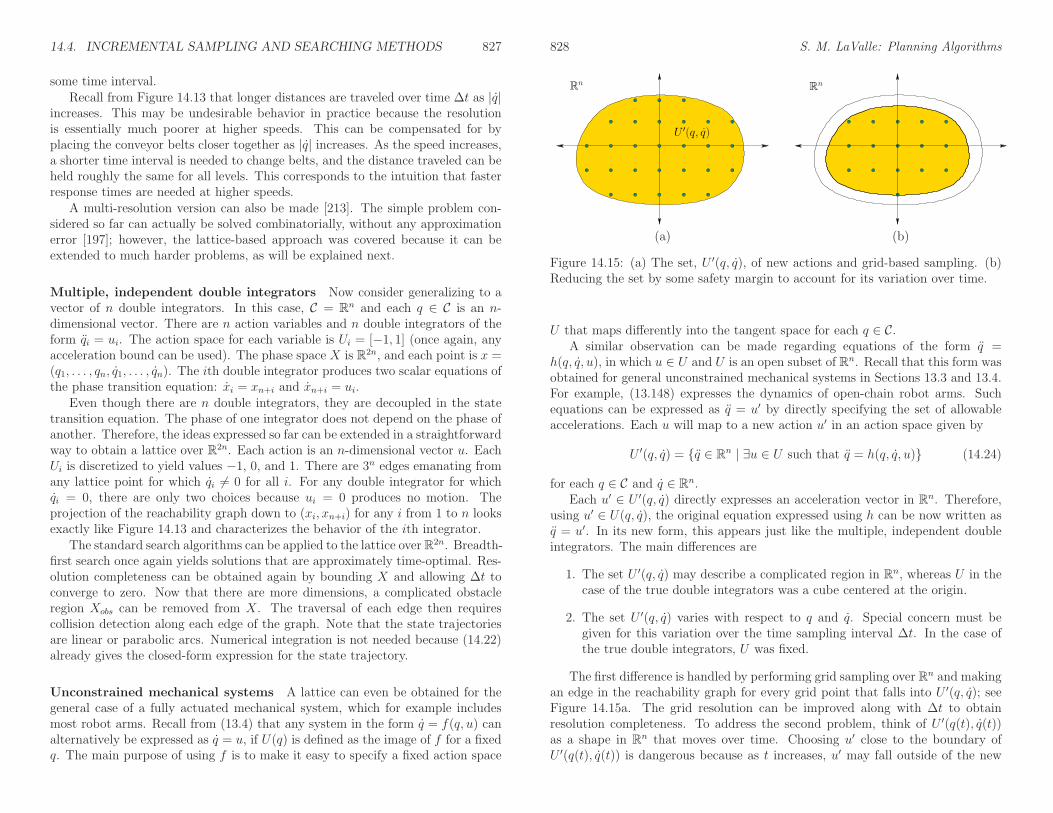
14.4. INCREMENTAL SAMPLING AND SEARCHING METHODS 827
some time interval.Recall from Figure 14.13 that longer distances are traveled over time ∆t as |q|
increases. This may be undesirable behavior in practice because the resolutionis essentially much poorer at higher speeds. This can be compensated for byplacing the conveyor belts closer together as |q| increases. As the speed increases,a shorter time interval is needed to change belts, and the distance traveled can beheld roughly the same for all levels. This corresponds to the intuition that fasterresponse times are needed at higher speeds.
A multi-resolution version can also be made [213]. The simple problem con-sidered so far can actually be solved combinatorially, without any approximationerror [197]; however, the lattice-based approach was covered because it can beextended to much harder problems, as will be explained next.
Multiple, independent double integrators Now consider generalizing to avector of n double integrators. In this case, C = R
n and each q ∈ C is an n-dimensional vector. There are n action variables and n double integrators of theform qi = ui. The action space for each variable is Ui = [−1, 1] (once again, anyacceleration bound can be used). The phase space X is R2n, and each point is x =(q1, . . . , qn, q1, . . . , qn). The ith double integrator produces two scalar equations ofthe phase transition equation: xi = xn+i and xn+i = ui.
Even though there are n double integrators, they are decoupled in the statetransition equation. The phase of one integrator does not depend on the phase ofanother. Therefore, the ideas expressed so far can be extended in a straightforwardway to obtain a lattice over R2n. Each action is an n-dimensional vector u. EachUi is discretized to yield values −1, 0, and 1. There are 3n edges emanating fromany lattice point for which qi 6= 0 for all i. For any double integrator for whichqi = 0, there are only two choices because ui = 0 produces no motion. Theprojection of the reachability graph down to (xi, xn+i) for any i from 1 to n looksexactly like Figure 14.13 and characterizes the behavior of the ith integrator.
The standard search algorithms can be applied to the lattice over R2n. Breadth-first search once again yields solutions that are approximately time-optimal. Res-olution completeness can be obtained again by bounding X and allowing ∆t toconverge to zero. Now that there are more dimensions, a complicated obstacleregion Xobs can be removed from X. The traversal of each edge then requirescollision detection along each edge of the graph. Note that the state trajectoriesare linear or parabolic arcs. Numerical integration is not needed because (14.22)already gives the closed-form expression for the state trajectory.
Unconstrained mechanical systems A lattice can even be obtained for thegeneral case of a fully actuated mechanical system, which for example includesmost robot arms. Recall from (13.4) that any system in the form q = f(q, u) canalternatively be expressed as q = u, if U(q) is defined as the image of f for a fixedq. The main purpose of using f is to make it easy to specify a fixed action space
828 S. M. LaValle: Planning Algorithms
U ′(q, q)
Rn
Rn
(a) (b)
Figure 14.15: (a) The set, U ′(q, q), of new actions and grid-based sampling. (b)Reducing the set by some safety margin to account for its variation over time.
U that maps differently into the tangent space for each q ∈ C.A similar observation can be made regarding equations of the form q =
h(q, q, u), in which u ∈ U and U is an open subset of Rn. Recall that this form wasobtained for general unconstrained mechanical systems in Sections 13.3 and 13.4.For example, (13.148) expresses the dynamics of open-chain robot arms. Suchequations can be expressed as q = u′ by directly specifying the set of allowableaccelerations. Each u will map to a new action u′ in an action space given by
U ′(q, q) = {q ∈ Rn | ∃u ∈ U such that q = h(q, q, u)} (14.24)
for each q ∈ C and q ∈ Rn.
Each u′ ∈ U ′(q, q) directly expresses an acceleration vector in Rn. Therefore,
using u′ ∈ U(q, q), the original equation expressed using h can be now written asq = u′. In its new form, this appears just like the multiple, independent doubleintegrators. The main differences are
1. The set U ′(q, q) may describe a complicated region in Rn, whereas U in the
case of the true double integrators was a cube centered at the origin.
2. The set U ′(q, q) varies with respect to q and q. Special concern must begiven for this variation over the time sampling interval ∆t. In the case ofthe true double integrators, U was fixed.
The first difference is handled by performing grid sampling over Rn and makingan edge in the reachability graph for every grid point that falls into U ′(q, q); seeFigure 14.15a. The grid resolution can be improved along with ∆t to obtainresolution completeness. To address the second problem, think of U ′(q(t), q(t))as a shape in R
n that moves over time. Choosing u′ close to the boundary ofU ′(q(t), q(t)) is dangerous because as t increases, u′ may fall outside of the new

14.4. INCREMENTAL SAMPLING AND SEARCHING METHODS 829
action set. It is often possible to obtain bounds on how quickly the boundary ofU ′(q, q) can vary over time (this can be determined, for example, by differentiatingh with respect to q and q). Based on the bound, a thin layer near the boundary ofU ′(q, q) can be removed from consideration to ensure that all attempted actionsremain in U ′(q(t), q(t)) during the whole interval ∆t. See Figure 14.15b.
These ideas were applied to extend the approximation algorithm framework tothe case of open-chain robot arms, for which h is given by (13.148). Suppose thatU is an axis-aligned rectangle, which is often the case for manipulators becausethe bounds for each ui correspond to torque limits for each motor. If q and qare fixed, then (13.140) applies a linear transformation to obtain q from u. Therectangle is generally sheared into a parallelepiped (a n-dimensional extension ofa parallelogram). Recall such transformations from Section 3.5 or linear algebra.
Approximation algorithm framework The lattices developed in this sectionwere introduced in [83] for analyzing the kinodynamic planning problem in therigorous approximation algorithm framework for NP-hard problems [199]. Supposethat there are two or three independent double integrators. The analysis showsthat the computed solutions are approximately optimal in the following sense. Letc0 and c1 be two positive constants that define a function
δ(c0, c1)(q) = c0 + c1‖q‖. (14.25)
Let tF denote the time at which the termination action is applied. A state tra-jectory is called δ(c0, c1)-safe if for all t ∈ [0, tF ], the ball of radius δ(c0, c1)(q)that is centered at q(t) does not cause collisions with obstacles in W . Note thatthe ball radius grows linearly as the speed increases. The robot can be imaginedas a disk with a radius determined by speed. Let xI , xG, c0, and c1 be given(only a point goal region is allowed). Suppose that for a given problem, thereexists a δ(c0, c1)-safe state trajectory (resulting from integrating any u ∈ U) thatterminates in xG after time topt. It was shown that by choosing the appropriate∆t (given by a formula in [83]), applying breadth-first search to the reachabilitylattice will find a (1− ǫ)δ(c0, c1)-safe trajectory that takes time at most (1+ ǫ)topt,and approximately connects xI to xG (which means that the closeness in X de-pends on ǫ). Furthermore, the running time of the algorithm is polynomial in 1/ǫand the number of primitives used to define polygonal obstacles.5 One of the keysteps in the analysis is to show that any state trajectory can be closely trackedusing only actions from Ud and keeping them constant over ∆t. One importantaspect is that it does not necessarily imply that the computed solution is close tothe true optimum, as it travels through X (only the execution times are close).Thus, the algorithm may give a solution from a different homotopy class from the
5One technical point: It is actually only pseudopolynomial [199] in amax, vmax, c0, c1, andthe width of the bounding cube in W. This means that the running time is polynomial ifthe representations of these parameters are treated as having constant size; however, it is notpolynomial in the actual number of bits needed to truly represent them.
830 S. M. LaValle: Planning Algorithms
one that contains the true optimal trajectory. The analysis was extended to thegeneral case of open-chain robot arms in [81, 121].
Backward and bidirectional versions There is a perfect symmetry to theconcepts presented so far in this section. A reachability lattice similar to theone in Figure 14.13 can be obtained by integrating backward in time. This in-dicates action sequences and associated initial states from which a fixed statecan be reached. Note that applying the ideas in the reverse direction does notrequire the system to be symmetric. Given that the graphs exist in both direc-tions, bidirectional search can be performed. By using the forward and backwardtime-limited reachability cones, the initial and goal states can be connected to acommon lattice, which is started, for example, at the origin.
Underactuated and nonholonomic systems Many interesting systems can-not be expressed in the form q = h(q, q, u) with n independent action variablesbecause of underactuation or other constraints. For example, the models in Sec-tion 13.1.2 are underactuated and nonholonomic. In this case, it is not straight-forward to convert the equations into a vector of double integrators because thedimension of U(q, q) is less than n, the dimension of C. This makes it impossibleto use grid-based sampling of U(q, q). Nevertheless, it is still possible in manycases to discretize the system in a clever way to obtain a lattice. If this can beobtained, then a straightforward resolution-complete approach based on classicalsearch algorithms can be developed. If X is bounded (or a bounded region isobtained after applying the phase constraints), then the search is performed on afinite graph. If failure occurs, then the resolution can be improved in the usualway to eventually obtain resolution completeness. As stated in Section 14.2.2,obtaining such a lattice is possible for a large family of nonholonomic systems[198]. Next, a method is presented for handling reachability graphs that are notlattices.
14.4.2 Incorporating State Space Discretization
If the reachability graph is not a lattice, which is typically the case with under-actuated and nonholonomic systems, then state space discretization can be usedto force it to behave like a lattice. If there are no differential constraints, thenpaths can be easily forced to travel along a lattice, as in the methods of Section7.7.1. Under differential constraints, the state cannot be forced, for example, tofollow a staircase path. Instead of sampling X and forcing trajectories to visitspecific points, X can be partitioned into small cells, within which no more thanone vertex is allowed in the search graph. This prevents a systematic search algo-rithm from running forever if the search graph has an infinite number of verticesin some bounded region. For example, with the Dubins car, if u is fixed to aninteger, an infinite number of vertices on a circle is obtained, as mentioned in

14.4. INCREMENTAL SAMPLING AND SEARCHING METHODS 831
Section 14.2.2. The ideas in this section are inspired mainly by the Barraquand-Latombe dynamic programming method [20], which has been mainly applied tothe models in Section 13.1.2. In the current presentation, however, the approachis substantially generalized. Here, optimality is not even necessarily required (butcan be imposed, if desired).
Decomposing X into cells At the outset, X is decomposed into a collection ofcells without considering collision detection. Suppose that X is an n-dimensionalrectangular subset of Rn. If X is more generally a smooth manifold, then therectangular subset can be defined in a coordinate neighborhood. If desired, iden-tifications can be used to respect the topology of X; however, coordinate changesare technically needed at the boundaries to properly express velocities (recall Sec-tion 8.3).
The most common cell decomposition is obtained by splittingX into n-dimensionalcubes of equal size by quantizing each coordinate. This will be called a cubical par-tition. Assume in general thatX is partitioned into a collectionD of n-dimensionalcells. Let D ∈ D denote a cell, which is a subset of X. It is assumed here that allcells have dimension n. In the case of cubes, this means that points on commonboundaries between cubes are declared to belong to only one neighboring cube(thus, the cells may be open, closed, or neither).
Note that X is partitioned into cells, and not Xfree, as might be expectedfrom the methods in Chapter 6. This means that collision detection and otherconstraints on X are ignored when defining D. The cells are defined in advance,just as grids were declared in Section 5.4.2. In the case of a cubical partition, thecells are immediately known upon quantization of each coordinate axis.
Searching The algorithm fits directly into the framework of Section 14.3.4. Asearch graph is constructed incrementally from xI by applying any systematicsearch algorithm. It is assumed that the system has been discretized in some way.Most often, the discrete-time model of Section 14.2.2 is used, which results in afixed ∆t and a finite set Ud of actions.
In the basic search algorithms of Section 2.2.1, it is important to keep track ofwhich vertices have been explored. Instead of applying this idea to vertices, it isapplied here to cells. A cell D is called visited if the search graph that has beenconstructed so far contains a vertex inD; otherwise, D is called unvisited. Initially,only the cell that contains xI is marked as visited. All others are initialized tounvisited. These labels are used to prune the reachability graph during the search,as shown in Figure 14.16.
The basic algorithm outline is shown in Figure 14.17. LetQ represent a priorityqueue in which the elements are vertices of the search graph. If optimization ofa cost functional is required, then Q may be sorted by the cost accumulatedalong the path constructed so far from xI to x. This cost can be assigned in manydifferent ways. It could simply represent the time (number of ∆t steps), or it could
832 S. M. LaValle: Planning Algorithms
(a) (b)
Figure 14.16: (a) The first four stages of a dense reachability graph for the Dubinscar. (b) One possible search graph, obtained by allowing at most one vertex percell. Many branches are pruned away. In this simple example, there are no celldivisions along the θ-axis.
count the number of times the action has changed. As the algorithm explores, newcandidate vertices are encountered. They are only saved in the search graph andplaced into Q if they lie in a cell marked unvisited and are violation-free. Uponencountering such a cell, it becomes marked as visited. The reached functiongenerates a set of violation-free trajectory segments. Under the discrete-timemodel, this means applying each u ∈ Ud over time ∆t and reporting only thosestates reached without violating the constraints (including collision avoidance).
As usual, the BVP issue may arise if XG is small relative to the cell size. IfXG is large enough to include entire cells, then this issue is avoided. If xG is asingle point, then it may only be possible to approximately reach xG. Therefore,the algorithm must accept reaching xG to within a specified tolerance. This canbe modeled by defining XG to be larger; therefore, tolerance is not explicitlymentioned.
Maintaining the cells There are several alternatives for maintaining the cells.The main operation that needs to be performed efficiently is point location [77]:determine which cell contains a given state. The original method in [20] preallo-cates an n-dimensional array. The collision-checking is even performed in advance.Any cell that contains at least one point in Xobs can be labeled as occupied. This

14.4. INCREMENTAL SAMPLING AND SEARCHING METHODS 833
CELL-BASED SEARCH(xI , xG)1 Q.insert(xI);2 G.init(xI);3 while Q 6= ∅ and xG is unvisited4 xcur → Q.pop();5 for each (ut, x) ∈ reached(xcur)6 if x is unvisited7 Q.insert(x);8 G.add vertex(x);9 G.add edge(ut);10 Mark cell that contains x as visited;11 Return G;
Figure 14.17: Searching by using a cell decomposition of X.
allows cells that contain collision configurations to be avoided without having tocall the collision detection module. For a fixed dimension, this scheme finds thecorrect cell and updates the labels in constant time. Unfortunately, the spacerequirement is exponential in dimension.
An alternative is to use a hash table to maintain the collection of cells thatare labeled as visited. This may be particularly valuable if optimality is notimportant and if it is expected that solutions will be found before most of thecells are reached. The point location problem can be solved efficiently withoutexplicitly storing a multi-dimensional array.
Suppose that the cubical decomposition is not necessarily used. One generalapproach is to define D as the Voronoi regions of a collection P of m samples{p1, . . . , pm} in X. The “name” of each cell corresponds uniquely to a samplein P . The cell that contains some x ∈ X is defined as the nearest sample in P ,using some predetermined metric on X. As a special case, the cubical decom-position defines the cells based on a Sukharev grid (recall Figure 5.5a). If thedimension of X is not too high, then efficient nearest-neighbor schemes can beused to determine the appropriate cell in near-logarithmic time in the numberof points in P (in practice, Kd-trees, mentioned in Section 5.5.2, should performwell). For maintaining a cubical decomposition, this approach would be cumber-some; however, it works for any sample set P . If no solution is found for a givenP , then the partition could be improved by adding more samples. This allows anydense sequence to be used to guide the exploration of X while ensuring resolutioncompleteness, which is discussed next.
Resolution issues One of the main complications in using state discretizationis that there are three spaces over which sampling occurs: time, the action space,and the state space. Assume the discrete-time model is used. If obtaining optimalsolutions is important, then very small cells should be used (e.g., 50 to 100 per
834 S. M. LaValle: Planning Algorithms
Uses minimum turning radius
Pruned away fromthe search graph
D
(a) (b)
Figure 14.18: (a) The Dubins car is able to turn around if it turns left as sharply aspossible. (b) Unfortunately, the required vertex is pruned because one cell alongthe required trajectory already contains a vertex. This illustrates how missing apossible action can cause serious problems many stages later.
axis). This limits its application to state spaces of a few dimensions. The timeinterval ∆t should also be made small, but if it is too small relative to the cell size,then it may be impossible to leave a cell. If only feasibility is the only requirement,then larger cells may be used, and ∆t must be appropriately increased. A coursequantization of U may cause solutions to be missed, particularly if ∆t is large. As∆t decreases, the number of samples in Ud becomes less important.
To obtain resolution completeness, the sampling should be improved each timethe search fails. Each time that the search is started, the sampling dispersion forat least one of the three spaces should be decreased. The possibilities are 1) thetime interval ∆t may be reduced, 2) more actions may be added to Ud, or 3) morepoints may be added to P to reduce the cell size. If the dispersion approaches zerofor all three spaces, and if XG contains an open subset of Xfree, then resolutioncompleteness is obtained. If XG is only a point, then solutions that come withinsome ǫ > 0 must be tolerated.
Recall that resolution completeness assumes that f has bounded derivativesor at least satisfies a Lipschitz condition (14.11). The actual rate of convergenceis mainly affected by three factors: 1) the rate at which f varies with respectto changes in u and x (characterized by Lipschitz constants), 2) the requiredtraversal of narrow regions in Xfree, and 3) the controllability of the system. Thelast condition will be studied further for nonholonomic systems in Section 15.4.

14.4. INCREMENTAL SAMPLING AND SEARCHING METHODS 835
For a concrete example, consider making a U-turn with a Dubins car that hasa very large turning radius, as shown in Figure 14.18. A precise turn may berequired to turn around, and this may depend on an action that was chosen manystages earlier. The Dubins car model does not allow zig-zagging (e.g., parallelparking) maneuvers to make local corrections to the configuration.
Backward and bidirectional versions As usual, both backward and bidi-rectional versions of this approach can be made. If the XG is large (or the goaltolerance is large) and the BVP is costly to solve, then the backward version seemsless desirable if the BVP is hard. The forward direction is preferred because theBVP can be avoided altogether.
For a bidirectional algorithm, the same collection D of cells can be used forboth trees. The problem could be considered solved if the same cell is reachedby both trees; however, one must be careful to still ensure that the remainingBVP can be solved. It must be possible to find an action trajectory segment thatconnects a vertex from the initial-based tree to a vertex of the goal-based tree.Alternatively, connections made to within a tolerance may be acceptable.
14.4.3 RDT-Based Methods
The rapidly exploring dense tree (RDT) family of methods, which includes theRRT, avoids maintaining a lattice altogether. RDTs were originally developed forhandling differential constraints, even though most of their practical applicationhas been to the Piano Mover’s Problem. This section extends the ideas of Section5.5 from C to X and incorporates differential constraints. The methods coveredso far in Section 14.4 produce approximately optimal solutions if the graph issearched using dynamic programming and the resolution is high enough. Bycontrast, RDTs are aimed at returning only feasible trajectories, even as theresolution improves. They are often successful at producing a solution trajectorywith relatively less sampling. This performance gain is enabled in part by the lackof concern for optimality.
Let α denote an infinite, dense sequence of samples in X. Let ρ : X × X →[0,∞] denote a distance function on X, which may or may not be a proper metric.The distance function may not be symmetric, in which case ρ(x1, x2) representsthe directed distance from x1 to x2.
The RDT is a search graph as considered so far in this section and can hencebe interpreted as a subgraph of the reachability graph under some discretizationmodel. For simplicity, first assume that the discrete-time model of Section 14.2.2is used, which leads to a finite action set Ud and a fixed time interval ∆t. Theset Up of motion primitives is all action trajectories for which some u ∈ Ud is heldconstant from time 0 to ∆t. The more general case will be handled at the end ofthis section.
Paralleling Section 5.5.1, the RDT will first be defined in the absence of ob-
836 S. M. LaValle: Planning Algorithms
SIMPLE RDT WITH DIFFERENTIAL CONSTRAINTS(x0)1 G.init(x0);2 for i = 1 to k do3 xn ← nearest(S(G), α(i));4 (up, xr)← local planner(xn, α(i));5 G.add vertex(xr);6 G.add edge(up);
Figure 14.19: Extending the basic RDT algorithm to handle differential con-straints. In comparison to Figure 5.16, an LPM computes xr, which becomes thenew vertex, instead of α(i). In some applications, line 4 may fail, in which caselines 5 and 6 are skipped.
Apply some up
xn
α(i)
Figure 14.20: If the nearest point S lies in the state trajectory segment associatedto an edge, then the edge is split into two, and a new vertex is inserted into G.
stacles. Hence, let Xfree = X. The construction algorithm is defined in Figure14.19; it may be helpful to compare it to Figure 5.16, which was introduced onC for the Piano Mover’s Problem. The RDT, denoted by G, is initialized with asingle vertex at some x0 ∈ X. In each iteration, a new edge and vertex are addedto G. Line 3 uses ρ to choose xn, which is the nearest point to α(i) in the swathof G. In the RDT algorithm of Section 5.5, each sample of α becomes a vertex.Due to the BVP and the particular motion primitives in Up, it may be difficult orimpossible to precisely reach α(i). Therefore, line 4 calls an LPM to determine aprimitive up ∈ Up that produces a new state xr upon integration from xn. Theresult is depicted in Figure 14.20. For the default case in which Up represents thediscrete-time model, the action is chosen by applying all u ∈ U over time ∆t andselecting the one that minimizes ρ(xr, α(i)). One additional constraint is that ifxn has been chosen in a previous iteration, then up must be a motion primitivethat has not been previously tried from xn; otherwise, duplicate edges would re-sult in G or time would be wasted performing collision checking for reachabilitygraph edges that are already known to be in collision. The remaining steps addthe new vertex and edge from xn. If xn is contained in the trajectory produced

14.4. INCREMENTAL SAMPLING AND SEARCHING METHODS 837
by an edge e, then e is split as described in Section 5.5.1.
Efficiently finding nearest points The issues of Section 5.5.2 arise again forRDTs under differential constraints. In fact, the problem is further complicatedbecause the edges in G are generally curved. This prevents the use of simplepoint-segment distance tests. Furthermore, an exact representation of the statetrajectory is usually not known. Instead, it is approximated numerically by thesystem simulator. For these reasons, it is best to use the approximate method ofdetermining the nearest point in the swath, which is a straightforward extensionof the discussion in Section 5.5.2; recall Figure 5.22. Intermediate vertices may beinserted if the applied motion primitive yields a state trajectory that travels farin Xfree. If the dimension is low enough (e.g., less than 20), then efficient nearest-neighbor algorithms (Section 5.5.2) can be used to offset the cost of maintainingintermediate vertices.
Handling obstacles Now suppose that Xobs 6= ∅. In Section 5.5.1, the RDTwas extended until a stopping configuration qs was reached, just in front of anobstacle. There are two new complications under differential constraints. The firstis that motion primitives are used. If ∆t is small, then in many cases the timewill expire before the boundary is reached. This can be alleviated by using a large∆t and then taking only the violation-free portion of the trajectory. In this case,the trajectory may even be clipped early to avoid overshooting α(i). The secondcomplication is due to Xric. If momentum is substantial, then pulling the tree asclose as possible to obstacles will increase the likelihood that the RDT becomestrapped. Vertices close to obstacles will be selected often because they have largeVoronoi regions, but expansion is not possible. In the case of the Piano Mover’sProblem, this was much less significant because the tree could easily follow alongthe boundary. In most experimental work, it therefore seems best to travel onlypart of the way (perhaps half) to the boundary.
Tree-based planners Planning algorithms can be constructed from RDTs inthe same way as in Section 5.5. Forward, backward, and bidirectional versionscan be made. The main new complication is the familiar BVP that the othersampling-based methods of this section have also suffered from. If it is expensiveor even impossible to connect nearby states, then the usual complications arise. IfXG contains a sizable open set, then a forward, single-tree planner with a gentlebias toward the goal could perform well while avoiding the BVP. However, if XG
is a point, then a tolerance must be set on how close the RDT must get to thegoal before it can declare that it has a solution. For systems with drift, the searchtime often increases dramatically as this tolerance decreases.
Bidirectional search offers great performance advantages in many cases, but theBVP exists when attempting connections between the two trees. One possibility isto set the tolerance very small and then concatenate the two action trajectories, as
838 S. M. LaValle: Planning Algorithms
described in Section 14.3.4. If it succeeds, then the planning algorithm successfullyterminates. Unfortunately, the performance once again depends greatly on thetolerance, particularly if the drift is substantial. Recent studies have shown thatusing a bidirectional RDT with a large connection tolerance and then closing thegap by using efficient variational techniques provides dramatic improvement inperformance [61, 154]. Unfortunately, variational techniques are not efficient forall systems because they must essentially solve the BVP by performing a gradientdescent in the trajectory space; see Section 14.7.
Distance function issues The RDT construction algorithm is heavily influ-enced by the distance function ρ. This was also true for RDTs applied to thePiano Mover’s Problem; however, it becomes more critical and challenging to de-sign a good metric in the presence of differential constraints. For example, themetric given by Example 5.3 is inappropriate for measuring the distance betweenconfigurations for the Dubins car. A more appropriate metric is to use lengthof the shortest path from q to q′ (this length is easy to compute; see Section15.5). Such a metric would be more appropriate than the one in Example 5.3for comparing the configurations, even for car models that involve dynamics andobstacles.
Although many challenging problems can be solved using weighted Euclideanmetrics [166], dramatic improvements can be obtained by exploiting particularproperties of the system. This problem might seem similar to the choice of a po-tential function for the randomized potential field planer of Section 5.4.3; however,since RDTs approach many different samples in α(i), instead of focusing only onthe goal, the performance degradation is generally not as severe as the local min-imum problem for a potential field planner. There are many more opportunitiesto escape in an RDT. Metrics that would fail miserably as a potential functionoften yield good performance in an RDT-based planner.
The ideal distance function, as mentioned in Section 14.3, is to use the optimalcost-to-go, denoted here as ρ∗. Of course, computing ρ∗ is at least as hard assolving the motion planning problem. Therefore, this idea does not seem practical.However, it is generally useful to consider ρ∗ because the performance of RDT-based planners generally degrades as ρ, the actual metric used in the RDT, andρ∗ diverge. An effort to make a crude approximation to ρ∗, even if obstaclesare neglected, often leads to great improvements in performance. An excellentexample of this appears in [104], in which value iteration was used to compute theoptimal cost-to-go in the absence of obstacles for an autonomous helicopter usingthe maneuver automaton model of Figure 14.8.
Ensuring resolution completeness Suppose that the discrete-time model isused. If α is dense in X, then each RDT vertex is visited a countably infinitenumber of times after it is constructed. By ensuring that the same motion prim-itive is never applied twice from the same vertex, all available motion primitives

14.4. INCREMENTAL SAMPLING AND SEARCHING METHODS 839
will eventually be tried. This ensures that the full reachability graph is exploredfor a fixed ∆t. Since the reachability graph is not necessarily finite, obtainingresolution completeness is more challenging. The scheme described in Figure 14.7can be applied by periodically varying ∆t during execution, and using smaller andsmaller of values of ∆t in later iterations. If U is finite, refinements can also bemade to Ud. This leads to a resolution-complete RDT.
Designing good motion primitives Up to this point, only the discrete-timemodel has been considered. Although it is the most straightforward and general,there are often many better motion primitives that can be used. For a particu-lar system, it may be possible to design a nice family of trajectories off-line inthe absence of obstacles and then use them as motion primitives in the RDTconstruction. If possible, it is important to carefully analyze the system underconsideration to try to exploit any special structure it may have or techniques thatmight have been developed for it. For motion planning of a vehicle, symmetriescan be exploited to apply the primitives from different states. For example, inflying a helicopter, the yaw angle and the particular position (unless it is close tothe ground) may not be important. A family of trajectories designed for one yawangle and position should work well for others.
Using more complicated motion primitives may increase the burden on theLPM. In some cases, a simple control law (e.g., PID [12]) may perform well. Ide-ally, the LPM should behave like a good steering method, which could be obtainedusing methods in Chapter 15. It is important to note, though, that the RDT’sability to solve problems does not hinge on this. It will greatly improve perfor-mance if there are excellent motion primitives and a good steering method in theLPM. The main reason for this is that the difficulties of the differential constraintshave essentially been overcome once this happens (except for the adverse effectsof drift). Although having good motion primitives can often improve performancein practice, it can also increase the difficulty of ensuring resolution completeness.
14.4.4 Other Methods
Extensions of virtually any other method in Chapter 5 can be made to handledifferential constraints. Several possibilities are briefly mentioned in this section.
Randomized potential fields The randomized potential field method of Sec-tion 5.4.3 can be easily adapted to handle differential constraints. Instead ofmoving in any direction to reduce the potential value, motion primitives are ap-plied and integrated to attempt to reduce the value. For example, under thediscrete-time model, each u ∈ Ud can be applied over ∆t, and the one for whichthe next state has the lowest potential value should be selected as part of thedescent. Random walks can be tried whenever no such action exists, but onceagain, motion in any direction is not possible. Random actions can be chosen
840 S. M. LaValle: Planning Algorithms
instead. The main problems with the method under differential constraints are1) it is extremely challenging to design a good potential function, and 2) randomactions do not necessarily provide motions that are similar to those of a randomwalk. Section 15.1.2 discusses Lyapunov functions, which serve as good potentialfunctions in the presence of differential constraints (but usually neglect obstacles).In the place of random walks, other planning methods, such as an RDT, could beused to try to escape local minima.
Other tree-based planners Many other tree-based planners can be extendedto handle differential constraints. For example, an extension of the expansive spaceplanner from Section 5.4.4 to kinodynamic planning for spacecrafts appears in[126]. Recently, a new tree-based method, called the path-directed subdivision tree,has been proposed for planning under differential constraints [151]. The methodworks by choosing points at random in the swath, applying random actions, andalso using a space-partition data structure to control the exploration.
Sampling-based roadmap planners As stated already, it is generally difficultto construct sampling-based roadmaps unless the BVP can be efficiently solved.The steering methods of Section 15.5 can serve this purpose [250, 226]. In prin-ciple, any of the single-query methods of Section 14.4 could be used; however, itmay be too costly to use them numerous times, which is required in the roadmapconstruction algorithm.
14.5 Feedback Planning Under Differential Con-
straints
14.5.1 Problem Definition
Formulation 14.1 assumed that feedback is not necessary. If the initial stateis given, then the solution takes the form of an action trajectory, which uponintegration yields a time-parametrized path through Xfree. This extended thePiano Mover’s Problem of Section 4.3.1 to include phase spaces and differentialconstraints. Now suppose that feedback is required. The reasons may be that theinitial state is not given or the plan execution might not be predictable due todisturbances or errors in the system model. Recall the motivation from Section8.1.
With little effort, the feedback motion planning framework from Chapter 8can be extended to handle differential constraints. Compare Formulations 8.2and 14.1. Feedback motion planning under differential constraints is obtained bymaking the following adjustments to Formulation 8.2:
1. In Formulation 8.2, X = Cfree, which automatically removed Cobs from C bydefinition. Now let X be any C-space or phase space, and let Xobs be defined

14.5. FEEDBACK PLANNING UNDER DIFFERENTIAL CONSTRAINTS841
as in Formulation 8.2. This leads to Xfree, as defined in Formulation 14.1.
2. In Formulation 8.2, the state transition equation was x = u, which directlyspecified velocities in the tangent space Tx(X). Now let any system, x =f(x, u), be used instead. In this case, U(x) is no longer a subset of Tx(X).It still includes the special termination action uT .
3. Formulation 14.1 includes xI , which is now removed for the feedback caseto be consistent with Formulation 8.2.
4. A feedback plan is now defined as a function π : Xfree → U . For a givenstate x ∈ Xfree, an action π(x) is produced. Composing π with f yieldsa velocity in Tx(X) given by x = f(x, π(x)). Therefore, π defines a vectorfield on Xfree.
Let tF denote the time at which uT is applied. Both feasible and optimal planningcan be defined using a cost functional,
L(xtF , utF ) =
∫ tF
0
l(x(t), u(t))dt+ lF (x(tF )), (14.26)
which is identical to that given in Section 8.4.1. This now specifies the problemof feedback motion planning under differential constraints.
The most important difference with respect to Chapter 8 is that x = u is re-placed with x = f(x, u), which allows complicated differential models of Chapter13 to be used. The vector field that results from π must satisfy the differen-tial constraints imposed by x = f(x, u). In Section 8.4.4, simple constraints onthe allowable vector fields were imposed, such as velocity bounds or smoothness;however, these constraints were not as severe as the models in Chapter 13. Forexample, the Dubins car does not allow motions in the reverse direction, whereasthe constraints in Section 8.4.4 permit motions in any direction.
14.5.2 Dynamic Programming with Interpolation
As observed in Section 14.4, motion planning under differential constraints isextremely challenging. Additionally requiring feedback complicates the problemeven further. If Xobs = ∅, then a feedback plan can be designed using numeroustechniques from control theory. See Section 15.2.2 and [58, 140, 221]. In manycases, designing feedback plans is no more difficult than computing an open-looptrajectory. However, if Xobs 6= ∅, feedback usually makes the problem muchharder.
Fortunately, dynamic programming once again comes to the rescue. In Sec-tion 2.3, value iteration yielded feedback plans for discrete state spaces and statetransition equations. It is remarkable that this idea can be generalized to the casein which U and X are continuous and there is a continuum of stages (called time).Most of the tools required to apply dynamic programming in the current setting
842 S. M. LaValle: Planning Algorithms
were already introduced in Section 8.5.2. The main ideas in that section were torepresent the optimal cost-to-go G∗ by interpolation and to use a discrete-timeapproximation to the motion planning problem.
The discrete-time model of Section 14.2.2 can be used in the current settingto obtain a discrete-stage state transition equation of the form xk+1 = fd(xk, uk).The cost functional is approximated as in Section 8.5.2 by using (8.65). Thisintegral can be evaluated numerically by using the result of the system simulatorand yields the cost-per-stage as ld(xk, uk). Using backward value iteration, thedynamic programming recurrence is
G∗k(xk) = min
uk∈Ud
{
ld(xk, uk) +G∗k+1(xk+1)
}
, (14.27)
which is similar to (2.11) and (8.56). The finite set Ud of action samples is usedif U is not already finite. The system simulator is applied to determine whethersome points along the trajectory lie in Xobs. In this case, ld(xk, uk) = ∞, whichprevents actions from being chosen that violate constraints.
As in Section 8.5.2, a set P ⊂ X of samples is used to approximate G∗ overX. The required values at points in X \ P are obtained by interpolation. Forexample, the barycentric subdivision scheme of Figure 8.20 may be applied hereto interpolate over simplexes in O(n lg n) time, in which n is the dimension of X.
As usual, backward value iteration starts at some final stage F and proceedsbackward through the stage indices. Termination occurs when all of the cost-to-govalues stabilize. The initialization at stage F yields G∗
F (x) = 0 for x ∈ XG ∩ P ;otherwise, G∗
F (x) = ∞. Each subsequent iteration is performed by evaluating(14.27) on each x ∈ P and using interpolation to obtain G∗
k+1(xk+1).The resulting stationary cost-to-go function G∗ can serve as a navigation func-
tion over Xfree, as described in Section 8.5.2. Recall from Chapter 8 that a nav-igation function is converted into a feedback plan by applying a local operator.The local operator in the present setting is
π(x) = argminu∈Ud
{
ld(x, u) +G∗(fd(x, u))}
, (14.28)
which yields an action for any state in Xfree that falls into an interpolation neigh-borhood of some samples in P .
Unfortunately, the method presented here is only useful in spaces of a fewdimensions. If X = C, then it may be applied, for example, to the systemsin Section 13.1.2. If dynamics are considered, then in many circumstances thedimension is too high because the dimension of X is usually twice that of C. Forexample, if A is a rigid body in the plane, then the dimension of X is six, whichis already at the usual limit of practical use.
It is interesting to compare the use of dynamic programming here with that ofSections 14.4.1 and 14.4.2, in which a search graph was constructed. If Dijkstra’salgorithm is used (or even breadth-first search in the case of time optimality), then

14.5. FEEDBACK PLANNING UNDER DIFFERENTIAL CONSTRAINTS843
by the dynamic programming principle, the resulting solutions are approximatelyoptimal. To ensure convergence, resolution completeness arguments were givenbased on Lipschitz conditions on f . It was important to allow the resolution toimprove as the search failed to find a solution. Instead of computing a searchgraph, value iteration is based on computing cost-to-go functions. In the sameway that both forward and backward versions of the tree-based approaches werepossible, both forward and backward value iteration can be used here. Providingresolution completeness is more difficult, however, because xI is not fixed. It istherefore not known whether some resolution is good enough for the intendedapplication. If xI is known, then G
∗ can be used to generate a trajectory from xIusing the system simulator. If the trajectory fails to reach XG, then the resolutioncan be improved by adding more samples to P and Ud or by reducing ∆t. UnderLipschitz conditions on f , the approach converges to the true optimal cost-to-go[26, 55, 148]. Therefore, value iteration can be considered resolution completewith respect to a given xI . The convergence even extends to computing optimalfeedback plans with additional actions that are taken by nature, which is modelednondeterministically or probabilistically. This extends the value iteration methodof Section 10.6.
The relationship between the methods based on a search graph and on valueiteration can be brought even closer by constructing Dijkstra-like versions of valueiteration, as described at the end of Section 8.5.2. These extend Dijkstra’s algo-rithm, which was viewed for the finite case in Section 2.3.3 as an improvement tovalue iteration. The improvement to value iteration is made by recognizing that inmost evaluations of (14.27), the cost-to-go value does not change. This is causedby two factors: 1) From some states, no trajectory has yet been found that leadsto XG; therefore, the cost-to-go remains at infinity. 2) The optimal cost-to-gofrom some state might already be computed; no future iterations would improvethe cost.
A forward or backward version of a Dijkstra-like algorithm can be made. Con-sider the backward case. The notion of a backprojection was used in Section8.5.2 to characterize the set of states that can reach another set of states in onestage. This was used in (8.68) to define the frontier during the execution of theDijkstra-like algorithm. There is essentially no difference in the current setting tohandle the system x = f(x, u). Once the discrete-time approximation has beenmade, the definition of the backprojection is essentially the same as in (8.66) ofSection 8.5.2. Using the discrete-time model of Section 14.2.2, the backprojectionof a state x ∈ Xfree is
B(x) = {x′ ∈ Xfree | ∃u ∈ Ud such that x = fd(x′, u)}. (14.29)
The backprojection is closely related to the backward time-limited reachable setfrom Section 14.2.1. The backprojection can be considered as a discrete, one-stageversion, which indicates the states that can reach x through the application of aconstant action u ∈ Ud over time ∆t. As mentioned in Section 8.5.2, comput-ing an overapproximation to the frontier set may be preferable in practice. This
844 S. M. LaValle: Planning Algorithms
can be obtained by approximating the backprojections, which are generally morecomplicated under differential constraints than for the case considered in Section8.5.2. One useful simplification is to ignore collisions with obstacles in definingB(x). Also, a simple bounding volume of the true backprojection may be used.The trade-offs are similar to those in collision detection, as mentioned in Section5.3.2. Sometimes the structure of the particular system greatly helps in determin-ing the backprojections. A nice wavefront propagation algorithm can be obtained,for example, for a double integrator; this is exploited in Section 14.6.3. For moreon value iteration and Dijkstra-like versions, see [165].
14.6 Decoupled Planning Approaches
14.6.1 Different Ways to Decouple the Big Problem
As sampling-based algorithms continue to improve along with computation power,it becomes increasingly feasible in practice to directly solve challenging planningproblems under differential constraints. There are many situations, however, inwhich computing such solutions is still too costly due to expensive numerical inte-gration, collision detection, and complicated obstacles in a high-dimensional statespace. Decoupled approaches become appealing because they divide the big prob-lem into modules that are each easier to solve. For versions of the Piano Mover’sProblem, such methods were already seen in Chapter 7. Section 7.1.3 introducedthe velocity-tuning method to handle time-varying obstacles, and Section 7.2.2presented decoupled approaches to coordinating multiple robots.
Ideally, we would like to obtain feedback plans on any state space in the pres-ence of obstacles and differential constraints. This assumes that the state canbe reliably measured during execution. Section 14.5 provided the best generictechniques for solving the problem, but they are unfortunately limited to a fewdimensions. If there is substantial sensing uncertainty, then the feedback planmust be defined on the I-space, which was covered in Chapter 11. Back in Section1.4, Figure 1.19 showed a popular model of decoupling the big planning prob-lem into a sequence of refinements. A typical decoupled approach involves fourmodules:
1. Use a motion planning algorithm to find a collision-free path τ : [0, 1] →Cfree.
2. Transform τ into a new path τ ′ so that velocity constraints on C (if there areany) are satisfied. This might, for example, ensure that the Dubins car canactually follow the path. At the very least, some path-smoothing is neededin most circumstances.
3. Compute a timing function σ : [0, tF ]→ [0, 1] for τ ′ so that τ ′ ◦ σ is a time-parameterized path through Cfree with the following requirement. The state

14.6. DECOUPLED PLANNING APPROACHES 845
trajectory x must satisfy x = f(x(t), u(t)) and u(t) ∈ U(x(t)) for all time,until uT is applied at time tF .
4. Design a feedback plan (or feedback control law) π : X → U that tracks x.The plan should attempt to minimize the error between the desired stateand the measured state during execution.
Given recent techniques and computation power, the significance of this approachmay diminish somewhat; however, it remains an important way to decompose andsolve problems. Be aware, however, that this decomposition is arbitrary. If everymodule can be solved, then it is sufficient for producing a solution; however, sucha decomposition is not necessary. At any step along the way, completeness maybe lost because of poor choices in earlier modules. It is often difficult for modulesto take into account problems that may arise later.
Various ways to merge the modules have been considered. The methods ofSection 14.4 solve either: 1) the first two modules simultaneously, if paths thatsatisfy q = f(q, u) are computed through Cfree, or 2) the first three modules simul-taneously, if paths that satisfy x = f(x, u) are computed through Xfree. Section14.5 solved all four modules simultaneously but was limited to low-dimensionalstate spaces.
Now consider keeping the modules separate. Planning methods from Part IIcan be applied to solve the first module. Section 14.6.2 will cover methods thatimplement the second module. Section 14.6.3 will cover methods that solve thethird module, possibly while also solving the second module. The fourth moduleis a well-studied control problem that is covered in numerous texts [140, 221, 224].
14.6.2 Plan and Transform
For the decoupled approach in this section, assume that X = C, which meansthere are only velocity constraints, as covered in Section 13.1. The system may bespecified as q = f(q, u) or implicitly as a set of constraints of the form gi(q, q) = 0.The ideas in this section can easily be extended to phase spaces. The method givenhere was developed primarily by Laumond (see [164]) and was also applied to thesimple car of Section 13.1.2 in [158]; other applications of the method are coveredin [164].
An outline of the plan-and-transform approach is shown in Figure 14.21. Inthe first step, a collision-free path τ : [0, 1] → Cfree is computed by ignoringdifferential constraints. The path is then iteratively modified until it satisfies theconstraints. In each iteration, a subinterval [s1, s2] ⊆ [0, 1] is selected by specifyingsome s1, s2 ∈ [0, 1] so that s1 < s2. These points may be chosen using randomsequences or may be chosen deterministically. The approach may use binarysubdivision to refine intervals and gradually improve the resolution on [0, 1] overthe iterations.
For each chosen interval [s1, s2], an LPM is used to compute a path segment γ :[0, 1]→ Cfree that satisfies the conditions γ(0) = τ(s1) and γ(1) = τ(s2). It might
846 S. M. LaValle: Planning Algorithms
PLAN-AND-TRANSFORM APPROACH
1. Compute a path τ : [0, 1] → Cfree using a motion planning algorithm, suchas one from Part II.
2. Choose some s1, s2 ∈ [0, 1] such that s1 < s2 and use an LPM to attempt toreplace the portion of τ from τ(s1) to τ(s2) with a path γ that satisfies thedifferential constraints.
3. If τ now satisfies the differential constraints over all [0, 1], then the algorithmterminates. Otherwise, go to Step 2.
Figure 14.21: A general outline of the plan-and-transform approach.
qG
qI
τ(s1) τ(s2)
τ
Figure 14.22: An initial path that ignores differential constraints.
be the case that the LPM fails because it cannot connect the two configurations ora collision may occur. In this case, another subinterval is chosen, and the processrepeats. Each time the LPM succeeds, τ is updated to τ ′ as
τ ′(s) =
τ(s) if s < s1γ((s− s1)/(s2 − s1)) if s ∈ [s1, s2]τ(s) if s > s2.
(14.30)
The argument to γ reparameterizes it to run from s1 to s2, instead of 0 to 1.
Example 14.5 (Plan-and-Transform for the Dubins Car) For a concreteexample, suppose that the task is to plan a path for the Dubins car. Figure 14.22shows a path τ that might be computed by a motion planning algorithm thatignores differential constraints. Two sharp corners cannot be traversed by thecar. Suppose that s1 and s2 are chosen at random, and appear at the locationsshown in Figure 14.22. The portion of τ between τ(s1) and τ(s2) needs to bereplaced by a path that can be executed by the Dubins car. Note that matchingthe orientations at τ(s1) and τ(s2) is important because they are part of theconfiguration.

14.6. DECOUPLED PLANNING APPROACHES 847
γ
τ(s1) τ(s2)
Figure 14.23: A path for the Dubins car can always be found by connecting abitangent to two circles generated by the minimum turning radius. The path isnot necessarily optimal; see Section 15.3.1 for optimal paths.
qG
qI
τ(s1) τ(s2)
Figure 14.24: Upon replacement, the resulting path τ ′ can be followed by theDubins car.
A replacement path γ is shown in Figure 14.23. This is obtained by implement-ing the following LPM. For the Dubins car, a path between any configurations canbe found by drawing circles at the starting and stopping configurations as shownin the figure. Each circle corresponds to the sharpest possible left turn or rightturn. It is straightforward to find a line that is tangent to one circle from eachconfiguration and also matches the direction of flow for the car (the circles arelike one-way streets). Using γ, the path τ is updated to obtain τ ′, which is shownin Figure 14.24, and satisfies the differential constraints for the Dubins car. Thisproblem was very simple, and in practice dozens of iterations may be necessary toreplace path segments. Also, if randomization is used, then intervals of the form[0, s] and [s, 1] must not be neglected.
�
Example 14.5 seemed easy because of the existence of a simple local planner.Also, there were no obstacles. Imagine that τ instead traveled through a narrow,
848 S. M. LaValle: Planning Algorithms
zig-zagging corridor. In this case, a solution might not even exist because ofsharp corners that cannot be turned by the Dubins car. If there had been an singleobstacle that happened to intersect the loop in Figure 14.24, then the replacementwould have failed. In general, there is no guarantee that the replacement segmentis collision-free. It is important for the LPM to construct path segments that areas close as possible to the original path. For the Dubins car, this is not possiblein many cases. For example, moving the Dubins car a small distance backwardrequires moving along the circles shown in Figure 14.23. Even as the distancebetween two configurations is reduced, the distance that the car needs to traveldoes not approach zero. This is true even if the shortest possible paths are usedfor the Dubins car.
What property should an LPM have to ensure resolution completeness of theplan-and-transform approach? A sufficient condition is given in [164]. Let ρdenote a metric on X. An LPM is said to satisfy the topological property if andonly if the following statement holds: For any ǫ > 0, there exists some δ > 0such that for any pair q, q′ ∈ Cfree having ρ(q, q′) < δ implies that ρ(τ(s), q) < ǫfor all s ∈ [0, 1]. If an LPM satisfies the topological property, then any collision-free path through Cfree can be transformed into one that satisfies the differentialconstraints. Suppose that a path τ has some clearance of at least ǫ in Cfree. Bydividing the domain of τ into intervals so that the change in q is no more thanδ over each interval, then the LPM will produce collision-free path segments forreplacement.
It turns out that for the Reeds-Shepp car (which has reverse) such an LPMcan be designed because it is small-time locally controllable, a property that willbe covered in Sections 15.1.3 and 15.4. In general, many techniques from Chapter15 may be useful for analyzing and designing effective LPMs.
An interesting adaptation of the plan-and-transform approach has been de-veloped for problems that involve k implicit constraints of the form gi(q, q) = 0.An outline of the multi-level approach, which was introduced in [226], is shownin Figure 14.25 (a similar approach was also introduced in [89]). The idea is tosort the k constraints into a sequence and introduce them one at a time. Initially,a path is planned that ignores the constraints. This path is first transformed tosatisfy g1(q, q) = 0 and avoid collisions by using the plan-and-transform methodof Figure 14.21. If successful, then the resulting path is transformed into onethat is collision-free and satisfies both g1(q, q) = 0 and g2(q, q) = 0. This processrepeats by adding one constraint each time, until either the method fails or all kconstraints have been taken into account.
14.6.3 Path-Constrained Trajectory Planning
This section assumes that a path τ : [0, 1] → Cfree has been given. It may becomputed by a motion planning algorithm from Part II or given by hand. Theremaining task is to determine the speed along the path in a way that satisfies

14.6. DECOUPLED PLANNING APPROACHES 849
MULTI-LEVEL APPROACH
1. Compute a path τ : [0, 1] → Cfree using a standard motion planning algo-rithm (as in Part II), and let i = 1.
2. Transform τ into a collision free path that satisfies gj(q, q) = 0 for all j from1 to i.
3. If the transformation failed in Step 2, then terminate and report failure.
4. If i < k, the number of implicit velocity constraints, then increment i andgo to Step 2. Otherwise, terminate and successfully report τ as a path thatsatisfies all constraints.
Figure 14.25: The multi-level approach considers implicit constraints one at atime.
differential constraints on the phase space X. Assume that each state x ∈ Xrepresents both a configuration and its time derivative, to obtain x = (q, q). Letn denote the dimension of C; hence, the dimension of X is 2n. Once a path isgiven, there are only two remaining degrees of freedom in X: 1) the positions ∈ [0, 1] along the domain of τ , and 2) the speed s = ds/dt at each s. Thefull state, x, can be recovered from these two parameters. As the state changes,it must satisfy a given system, x = f(x, u). It will be seen that a 2D planningproblem arises, which can be solved efficiently using many alternative techniques.Similar concepts appeared for decoupled versions of time-varying motion planningin Section 7.1. The presentation in the current section is inspired by work in time-scaling paths for robot manipulators [124, 230, 233], which was developed a coupleof decades ago. At that time, computers were much slower, which motivated thedevelopment of strongly decoupled approaches.
Expressing systems in terms of s, s, and s
Suppose that a system is given in the form
q = h(q, q, u), (14.31)
in which there are n action variables u = (u1, . . . , un). It may be helpful to glanceahead to Example 14.6, which will illustrate the coming concepts for the simplecase of double integrators q = u. The acceleration in C is determined from the statex = (q, q) and action u. Assume u ∈ U , in which U is an n-dimensional subset ofRn. If h is nonsingular at x, then an n-dimensional set of possible accelerations
arises from choices of u ∈ U . This means it is fully actuated. If there were fewerthan n action variables, then there would generally not be enough freedom tofollow a specified path. Therefore, U must be n-dimensional. Which choices of
850 S. M. LaValle: Planning Algorithms
u, however, constrain the motion to follow the given path τ? To determine this,the q, q, and q variables need to be related to the path domain s and its first andsecond time derivatives s and s, respectively. This leads to a subset of U thatcorresponds to actions that follow the path.
Suppose that s, s, s, and a path τ are given. The configuration q ∈ Cfree is
q = τ(s). (14.32)
Assume that all first and second derivatives of τ exist. The velocity q can bedetermined by the chain rule as
q =dτ
ds
ds
dt=dτ
dss, (14.33)
in which the derivative dτ/ds is evaluated at s. The acceleration is obtained bytaking another derivative, which yields
q =d
dt
(
dτ
dss
)
=d2τ
ds2ds
dts+
dτ
dss
=d2τ
ds2s2 +
dτ
dss,
(14.34)
by application of the product rule. The full state x = (q, q) can be recovered from(s, s) using (14.32) and (14.33).
The next step is to obtain an equation that looks similar to (14.31), but isexpressed in terms of s, s, and s. A function h′(s, s, u) can be obtained fromh(q, q, u) by substituting τ(s) for q and the right side of (14.33) for q:
h′(s, s, u) = h(τ(s),dτ
dss, u). (14.35)
This yieldsq = h′(s, s, u). (14.36)
For a given state x (which can be obtained from s and s), the set of accelerationsthat can be obtained by a choice of u in (14.36) is the same as that for the originalsystem in (14.31). The only difference is that x is now constrained to a 2D subsetof X, which are the states that can be reached by selecting values for s and s.
Applying (14.34) to the left side of (14.36) constrains the accelerations to causemotions that follow τ . This yields
d2τ
ds2s2 +
dτ
dss = h′(s, s, u), (14.37)
which can also be expressed as
dτ
dss = h′(s, s, u)− d2τ
ds2s2, (14.38)

14.6. DECOUPLED PLANNING APPROACHES 851
Cfree
τ(1)
τ(0) τ(2/3)
τ(1/3)
Figure 14.26: A bad path for path-constrained trajectory planning.
by moving the first term of (14.34) to the right. Note that n equations are actuallyrepresented in (14.38). For each i in which dτi/ds 6= 0, a constraint of the form
s =1
dτi/dsh′i(s, s, ui)−
d2τids2
s2 (14.39)
is obtained by solving for s.
Determining the allowable accelerations
The actions in U that cause τ to be followed can now be characterized. An actionu ∈ U follows τ if and only if every equation of the form (14.39) is satisfied. Ifdτi/ds 6= 0 for all i from 1 to n, then n such equations exist. Suppose that u1 ischosen, and the first equation is solved for s. The required values of the remainingaction variables u2, . . ., un can be obtained by substituting the determined s valueinto the remaining n− 1 equations. This means that the actions that follow τ areat most a one-dimensional subset of U .
If dτi/ds = 0 for some i, then following the path requires that qi = 0. Insteadof (14.39), the constraint is that hi(q, q, u) = 0. Example 14.6 will provide asimple illustration of this. If dτi/ds = 0 for all i, then the configuration is notallowed to change. This occurs in the degenerate (and useless) case in which τ isa constant function.
In many cases, a value of u does not exist that satisfies all of the constraintequations. This means that the path cannot be followed at that particular state.Such states should be removed, if possible, by defining phase constraints on X.By a poor choice of path τ violating such a phase constraint may be unavoidable.There may exist some s for which no u ∈ U can follow τ , regardless of s.
Even if a state trajectory may be optimal in some sense, its quality ultimatelydepends on the given path τ : [0, 1] → Cfree. Consider the path shown in Fig-ure 14.26. At τ(1/3), a “corner” is reached. This violates the differentiabilityassumption and would require infinite acceleration to traverse while remaining onτ . For some models, it may be possible to stop at τ(1/3) and then start again.For example, imagine a floating particle in the plane. It can be decelerated to
852 S. M. LaValle: Planning Algorithms
rest exactly at τ(1/3) and then started in a new direction to exactly follow thecurve. This assumes that the particle is fully actuated. If there are nonholonomicconstraints on C, as in the case of the Dubins car, then the given path must atleast satisfy them before accelerations can be considered. The solution in this casedepends on the existence of decoupling vector fields [52, 71].
It is generally preferable to round off any corners that might have been pro-duced by a motion planning algorithm in constructing τ . This helps, but it stilldoes not completely resolve the issue. The portion of the path around τ(2/3) isnot desirable because of high curvature. At a fixed speed, larger accelerationsare generally needed to follow sharp turns. The speed may have to be decreasedsimply because τ carelessly requires sharp turns in C. Imagine developing anautonomous double-decker tour bus. It is clear that following the curve aroundτ(2/3) may cause the bus to topple at high speeds. The bus will have to slowdown because it is a slave to the particular choice of τ .
The path-constrained phase space
Recall the approach in Section 14.4.1 that enabled systems of the form q =h(q, q, u) to be expressed as q = u′ for some suitable U ′(q, q) ⊆ U (this wasillustrated in Figure 14.15). This enabled many systems to be imagined as mul-tiple, independent double integrators with phase-dependent constraints on theaction space. The same idea can be applied here to obtain a single integrator.
Let S denote a 2D path-constrained phase space, in which each element is ofthe form (s, s) and represents the position and velocity along τ . This parame-terizes a 2D subset of the original phase space X. Each original state vector isx = (q, q) = (τ(s), dτ/ds s). Which accelerations are possible at points in S? Ateach (s, s), a subset of U can be determined that satisfies the equations of theform (14.39). Each valid action yields an acceleration s. Let U ′(s, s) ⊆ R denotethe set of all values of s that can be obtained from an action u ∈ U that satisfies(14.39) for each i (except the ones for which dτi/ds = 0). Now the system can beexpressed as s = u′, in which u′ ∈ U ′(s, s). After all of this work, we have arrivedat the double integrator. The main complication is that U ′(s, s) can be challeng-ing to determine for some systems. It could consist of a single interval, disjointintervals, or may even be empty. Assuming that U ′(s, s) has been characterized,it is straightforward to solve the remaining planning problem using techniquesalready presented in this chapter. One double integrator is not very challenging;hence, efficient sampling-based algorithms exist.
An obstacle region Sobs ⊂ S will now be considered. This includes any statesthat belong to Xfree. Given s and s, the state x can be computed to determinewhether any constraints on X are violated. Usually, τ is constructed to avoidobstacle collision; however, some phase constraints may also exist. The obstacleregion Sobs also includes any points (s, s) for which U ′(s, s) is empty. Let Sfreedenote S \ Sobs.
Before considering computation methods, we give some examples.

14.6. DECOUPLED PLANNING APPROACHES 853
Example 14.6 (Path-Constrained Double Integrators) Consider the caseof two double integrators. This could correspond physically to a particle movingin R
2. Hence, C = W = R2. Let U = [−1, 1]2 and q = u for u ∈ U . The
path τ will be chosen to force the particle to move along a line. For linear paths,dτ/ds is constant and d2τ/ds2 = 0. Using these observations and the fact thath′(s, s, u) = u, (14.39) simplifies to
s =ui
dτi/ds, (14.40)
for i = 1, 2.Suppose that τ(s) = (s, s), which means that the particle must move along a
diagonal line through the origin of C. This further simplifies (14.40) to s = u1 ands = u2. Hence any u1 ∈ [−1, 1] may be chosen, but u2 must then be chosen asu2 = u1. The constrained system can be written as one double integrator s = u′,in which u′ ∈ [−1, 1]. Both u1 and u2 are derived from u′ as u1 = u2 = u′. Notethat U ′ does not vary over S; this occurs because a linear path is degenerate.
Now consider constraining the motion to a general line:
τ(s) = (a1s+ b1, a2s+ b2), (14.41)
in which a1 and a2 are nonzero. In this case, (14.40) yields s = u1/a1 and s =u2/a2. Since each ui ∈ [−1, 1], each equation indicates that s ∈ [−1/ai, 1/ai]. Theacceleration must lie in the intersection of these two intervals. If |a1| ≥ |a2|, thens ∈ [−1/a1, 1/a1]. We can designate u′ = u1 and let u2 = u′a2/a1. If |a1| > |a2|,then s ∈ [−1/a2, 1/a2], u′ = u2, and u1 = u′a1/a2.
Suppose that a1 = 0 and a2 6= 0. The path is
τ(s) = (q1, a2s+ b2), (14.42)
in which q1 is fixed and the particle is constrained to move along a vertical linein C = R
2. In this case, only one constraint, s = u2, is obtained from (14.40).However, u1 is independently constrained to u1 = 0 because horizontal motionsare prohibited.
If n independent, double integrators are constrained to a line, a similar resultis obtained. There are n equations of the form (14.40). The i ∈ {1, . . . , n} forwhich |ai| is largest determines the acceleration range as s ∈ [−1/ai, 1/ai]. Theaction u′ is defined as u′ = ui, and the uj for j 6= i are obtained from the remainingn− 1 equations.
Now assume τ is nonlinear, in which case (14.39) becomes
s =ui
dτi/ds− d2τids2
s2, (14.43)
for each i for which dτi/ds 6= 0. Now the set U ′(s, s) varies over S. As thespeed s increases, it becomes less likely that U ′(s, s) is nonempty. In other words,
854 S. M. LaValle: Planning Algorithms
it is less likely that a solution exists to all equations of the form (14.43). In aphysical system, that means that staying on the path requires turning too sharply.At a high speed, this may require an acceleration q that lies outside of [−1, 1]n. �
The same ideas can be applied to systems that are much more complicated.This should not be surprising because in Section 14.4.1 systems of the form q =h(q, q) were interpreted as multiple, independent double integrators of the formq = u′, in which u′ ∈ U ′(q, q) provided the possible accelerations. Under thisinterpretation, and in light of Example 14.6, constraining the motions of a generalsystem to a path τ just further restricts U ′(q, q). The resulting set of allowableaccelerations may be at most one-dimensional.
The following example indicates the specialization of (14.39) for a robot arm.
Example 14.7 (Path-Constrained Manipulators) Suppose that the sys-tem is described as (13.142) from Section 13.4.2. This is a common form that hasbeen used for controlling robot arms for decades. Constraints of the form (14.39)can be derived by expressing q, q, and q in terms of s, s, and s. This requiresusing (14.32), (14.33), and (14.34). Direct substitution into (13.142) yields
M(τ(s))
(
d2τ
ds2s2 +
dτ
dss
)
+ C(
τ(s),dτ
dss)dτ
dss+ g(τ(s)) = u. (14.44)
This can be simplified to n equations of the form
αi(s)s+ βi(s)s2 + γi(s)s = ui. (14.45)
Solving each one for s yields a special case of (14.39). As in Example 14.6, eachequation determines a bounding interval for s. The intersection of the intervalsfor all n equations yields the allowed interval for s. The action u′ once againindicates the acceleration in the interval, and the original action variables ui canbe obtained from (14.45). If dτi/ds = 0, then αi(s) = 0, which corresponds to thecase in which the constraint does not apply. Instead, the constraint is that thevector u must be chosen so that qi = 0. �
Computing optimal solutions via dynamic programming
Dynamic programming with interpolation, as covered in Section 14.5, can beapplied to solve the problem once it is formulated in terms of the path-constrainedphase space S ⊂ R
2. The domain of τ provides the constraint 0 ≤ s ≤ 1.Assume that only forward progress along the path is needed; moving in the reversedirection should not be necessary. This implies that s > 0. To make S bounded,an upper bound, smax, is usually assumed, beyond which it is known that thespeed is too high to follow the path.

14.6. DECOUPLED PLANNING APPROACHES 855
s
s
smax
Sobs
Sobs
0 10
s
s0 1
(a) (b)
Figure 14.27: (a) Planning occurs in the path-constrained phase space. (b) Dueto the forward-progress assumption, value iteration can be reduced to a quickwavefront propagation across regularly spaced vertical lines in S.
This results in the planning problem shown in Figure 14.27a. The system isexpressed as s = u′, in which u′ ∈ U ′(s, s). The initial phase in S is (0, si) andthe goal phase is (1, sg). Typically, si = sg = 0. The region shown in Figure 14.27is contained in the first quadrant of the phase space because only positive valuesof s and s are allowed (in Figure 14.13, q and q could be positive or negative).This implies that all motions are to the right. The actions determine whetheraccelerations or decelerations will occur.
Backward value iteration with interpolation can be easily applied by discretiz-ing S and U ′(s, s). Due to the constraint s > 0, making a Dijkstra-like versionof the algorithm is straightforward. A simple wavefront propagation can even beperformed, starting at s = 1 and progressing backward in vertical waves untils = 0 is reached. See Figure 14.27b. The backprojection (14.29) can be greatlysimplified. Suppose that the s-axis is discretized into m+ 1 regularly spaced val-ues s0, . . ., sm at every ∆s, for some fixed ∆s > 0. Thus, sk = (k∆s)/m. Theindex k can be interpreted as the stage. Starting at k = m, the final cost-to-goG∗m(sm, sm) is defined as 0 if the corresponding phase represents the goal, and ∞
otherwise. At each sk, the s values are sampled, and the cost-to-go function isrepresented using one-dimensional linear interpolation along the vertical axis. Ateach stage, the dynamic programming computation
G∗k(sk, sk) = min
u′∈U ′(sk,sk)
{
l′d(sk, sk, u′) +G∗
k+1(sk+1, sk+1)}
(14.46)
is performed at each s sample. This represents a special form of (14.27). Linearinterpolation over discretized s values is used to evaluate G∗
k+1(sk+1, sk+1). The
856 S. M. LaValle: Planning Algorithms
cost term l′d is obtained from ld by computing the original state x ∈ X froms and s; however, if the trajectory segment enters Sobs, it receives infinite cost.The computations proceed until stage k = 1, at which time the optimal cost-to-goG∗
1(s1, s1) is computed. The optimal trajectory is obtained by using the cost-to-gofunction at each stage as a navigation function.
The dynamic programming approach is so general that it can even be extendedto path-constrained trajectory planning in the presence of higher order constraints[234]. For example, if a system is specified as q(3) = h(q, q, q, u), then a 3D path-constrained phase space results, in which each element is expressed as (s, s, s).The actions in this space are jerks, yielding s(3) = u′ for u′ ∈ U ′(s, s, s).
A bang-bang approach for time optimality
The dynamic programming approach is already very efficient because the searchis confined to two dimensions. Nevertheless, trajectories that are time optimalcan be computed even more efficiently if Sobs has some special structure. Theidea is to find an alternating sequence between two motion primitives: one ofmaximum acceleration and one of maximum deceleration. This kind of switchingbetween extreme opposites is often called bang-bang control and arises often inthe development of time-optimal control laws (look ahead to Example 15.4). Themethod explained here was introduced in [38, 233]. One drawback of obtainingtime-optimal trajectories is that they cannot be tracked (the fourth module fromSection 14.6.1) if errors occur because the solutions travel on the boundary of thereachable set.
The approach was developed for robot arms, as considered in Example 14.7.Suppose that Sobs is a single connected component that is bounded above by smax,and on the sides it is bounded by s = 0 and s = 1. It is assumed that S arisesonly due to the vanishing of the interval of allowable values for s (in this case,U ′(s, s) becomes empty). It is also assumed that the lower boundary of Sobs can beexpressed as a differentiable function φ : [0, 1]→ S, called the limit curve, whichyields the maximum speed s = φ(s) for every s ∈ [0, 1]. The method is extendedto handle multiple obstacles in [233], but this case is not considered here. Assumealso that dτi/ds 6= 0 for every i; the case of dτi/ds = 0 can also be handled in themethod [232].
Let u′min(s, s) and u′max(s, s) denote the smallest and largest possible acceler-
ations, respectively, from (s, s) ∈ S. If (s, s) 6∈ Sobs, then u′min(s, s) < u′max(s, s).At the limit curve, u′min(s, φ(s)) = u′max(s, φ(s)). Applying the only feasible actionin this case generates a velocity that is tangent to the limit curve. This is calleda tangent point, (stan, stan), to φ. Inside of Sobs, no accelerations are possible.
The bang-bang approach is described in Figure 14.28, and a graphical illustra-tion appears in Figure 14.29. Assume that the initial and goal phases are (0, 0)and (1, 0), respectively. Step 1 essentially enlarges the goal by constructing amaximum-deceleration curve that terminates at (1, 0). A trajectory that con-tacts this curve can optimally reach (1, 0) by switching to maximum deceleration.

14.6. DECOUPLED PLANNING APPROACHES 857
BANG-BANG APPROACH
1. From the final state (1, 0), apply reverse-time integration to s = u′min(s, s).Continue constructing the curve numerically until either the interior of Sobsis entered or s = 0. In the latter case, the algorithm terminates with failure.
2. Let (scur, scur) = (0, 0).
3. Apply forward integration s = u′max(s, s) from (scur, scur) until either theinterior of Sobs is entered or the curve generated in Step 1 is crossed. In thelatter case, the problem is solved.
4. Starting at the point where the trajectory from Step 3 crossed the limitcurve, find next tangent point (stan, stan) to the right along the limit curve.From (stan, stan), perform reverse integration on s = u′min(s, s) until thecurve from Step 3 is hit. Let (scur, scur) = (stan, stan) and go to Step 3.
Figure 14.28: The bang-bang approach finds a time-optimal, path-constrainedtrajectory with less searching than the dynamic programming approach.
s
s
0 1
Sobs
Figure 14.29: An illustration of the bang-bang approach to computing a time-optimal trajectory. The solution trajectory is obtained by connecting the dots.
858 S. M. LaValle: Planning Algorithms
Steps 3 and 4 construct a maximum-acceleration curve followed by a maximum-deceleration curve. The acceleration curve runs until it pierces the limit curve.This constraint violation must be avoided. Therefore, a deceleration must be de-termined that departs earlier from the acceleration curve and just barely missesentering the interior of Sobs. This curve must become tangent to the limit curve;therefore, a search is made along the limit curve for the next possible tangentpoint. From there, reverse-time integration is used in Step 4 to generate a de-celeration curve that contacts the acceleration curve. A portion of the solutionhas now been obtained in which an acceleration is followed by a deceleration thatarrives at a tangent point of φ. It is possible that Step 4 is not reached becausethe curve that connects to the goal is contacted. Starting from the tangent point,Steps 3 and 4 are repeated until the goal curve is contacted.
14.7 Gradient-Based Trajectory Optimization
This section provides a brief overview of a complementary problem to motionplanning. Suppose that an algorithm in this chapter returns a feasible actiontrajectory. How can the solution be improved? Trajectory optimization refers tothe problem of perturbing the trajectory while satisfying all constraints so that itsquality can be improved. For example, it may be desirable to shorten a trajectorycomputed by an RRT, to remove some of the arbitrary changes in actions due torandomization. Trajectory optimization is considered complementary to motionplanning because it usually requires an initial guess, which could be provided by aplanning algorithm. Trajectory optimization can be considered as a kind of BVP,but one that improves an initial guess, as opposed to determining trajectoriesfrom scratch.
The optimization issue also exists for paths computed by sampling-based algo-rithms for the Piano Mover’s Problem; however, without differential constraints,it is much simpler to shorten paths. The plan and transform method of Section14.6.2 can be applied, and the LPM just connects pairs of configurations alongthe shortest path in C. In the presence of differential constraints, the BVP mustbe faced.
In the most general setting, it is very difficult to improve trajectories. Thereare numerous methods from optimization literature; see [28, 48, 176] for overviews.The purpose of this section is to encourage further study by briefly mentioning thevarious kinds of methods that have been developed, instead of explaining themin detail. The methods fall under the area of nonlinear programming (NLP) (ornonlinear optimization), as opposed to linear programming, which was used to findrandomized security strategies in Section 9.3. The optimization actually occursin a space of possible trajectories, each of which is a function of time. Therefore,the calculus of variations, which was used in Section 13.4.1, becomes relevantto characterize extrema. The functional Φ from that setting becomes the costfunctional L in the current setting. The system x = f(x, u) forms an additional
14.7. GRADIENT-BASED TRAJECTORY OPTIMIZATION 859
set of constraints that must be satisfied, but u can be selected in the optimization.To enable numerical computation methods, a family of trajectories is speci-
fied in terms of a parameter space. The optimization can then be viewed as anincremental search in the parameter space while satisfying all constraints. Thedirection of motion in each step is determined by computing the gradient of acost functional with respect to the parameters while constrained to move in adirection tangent to the constraints. Hence, much of nonlinear programming canbe considered as an application of Newton’s method or gradient descent. As instandard optimization, second-order derivatives of the cost functional can be usedto indicate when the search should terminate. The numerical issues associatedwith these methods are quite involved; several NLP software packages, such asthe NAG Fortran Library or packages within Matlab, are available.
Nonlinear optimal control theory can be considered as a variant of NLP.The dynamic programming recurrence becomes a differential equation in thecontinuous-time setting, and Hamilton’s equations (13.198) generalize to Pontrya-gin’s minimum principle. These are covered in Section 15.2. The extra variablesthat arise in the minimum principle can be considered as Lagrange multipliers ofa constrained optimization, in which x = f(x, u) is the constraint. The differen-tial equations arising from dynamic programming or the minimum principle aredifficult to solve analytically; therefore, in most cases, numerical techniques areused. The case of numerical dynamic programming was covered in Section 14.5.
Shooting methods constitute the simplest family of trajectory optimizationmethods. As a simple example, suppose that an action trajectory u : [0, tF ]→ R
has been computed of the form
u(t) = w1 + w2t, (14.47)
in which w1 and w2 are some fixed parameters. Consider perturbing w1 and w2
by some small amount and applying the integration in (14.1). If f satisfies Lip-schitz conditions, then a small perturbation should produce a small change inx. The resulting new trajectory can be evaluated by a cost functional to deter-mine whether it is an improvement. It might, for example, have lower maximumcurvature. Rather than picking a perturbation at random, the gradient of thecost functional with respect to the parameters can be computed. A small stepin the parameter space along the negative gradient direction should reduce thecost. It is very likely, however, that perturbing w1 and w2 will move the final statex(tF ). Usually, a termination condition, such as x(tF ) = xG, must be enforcedas a constraint in the optimization. This removes degrees of freedom from theoptimization; therefore, more trajectory parameters are often needed.
Suppose more generally that a motion planning algorithm computes an actionsequence based on the discrete-time model. Each action in the sequence remainsconstant for duration ∆t. The time duration of each action can instead be definedas a parameter to be perturbed. Each action variable ui over each interval couldalso be perturbed using by (14.47) with the initial condition that w1 = ui and
860 S. M. LaValle: Planning Algorithms
w2 = 0. The dimension of the search has increased, but there are more degrees offreedom. In some formulations, the parameters may appear as implicit constraints;in this case, a BVP must be solved in each iteration. The minimum principleis often applied in this case [28]. More details on formulating and solving thetrajectory optimization problem via shooting appear in [48].
Several difficulties are encountered when applying the shooting technique totrajectory optimization among obstacles. Each perturbation requires integrationand collision-checking. For problems involving vehicles, the integrations can some-times be avoided by exploiting symmetries [60]. For example, a path for the Du-bins car can be perturbed by changing a steering angle over a short amount oftime, and the rest of the trajectory can simply be transformed using a matrix ofSE(2). A critical problem is that following the negative gradient may suggestshortening the path in a way that causes collision. The problem can be alleviatedby breaking the trajectory into segments, as in the plan-and-transform approach;however, this yields more optimizations. Another possible solution is to invent apenalty function for the obstacles; however, this is difficult due to local minimaproblems and the lack of representing the precise boundary of Xobs.
Another difficulty with shooting is that a small change in the action near thestarting time may lead to great changes in the states at later times. One wayto alleviate this problem is by multiple shooting (as opposed to single shooting,which has been described so far). In this case, the trajectory is initially brokeninto segments. These could correspond to the time boundaries imposed by asequence of motion primitives. In this case, imagine perturbing each motionprimitive separately. Extra constraints are needed in this case to indicate that allof the trajectory pieces must remain connected. The multiple shooting methodcan be generalized to a family of methods called transcription or collocation (see[28] for references). These methods again split the trajectory into segments, buteach connection constraint relates more points along the trajectory than just thesegment endpoints. One version of transcription uses implicit constraints, whichrequire using another BVP solver, and another version uses parametric constraints,which dramatically increases the dimension of the search. The latter case is stilluseful in practice by employing fast, sparse-matrix computation methods.
One of the main difficulties with trajectory optimization methods is that theycan become stuck in a local minimum in the space of trajectories. This means thattheir behavior depends strongly on the initial guess. It is generally impossible forthem to find a trajectory that is not homotopic to the initial trajectory. Theycannot recover from an initial guess in a bad homotopy class. If Xobs is compli-cated, then this issue becomes increasingly important. In many cases, variationaltechniques might not even find an optimal solution within a single homotopy class.Multiple local minima may exist if the closure of Xfree contains positive curvature.If it does not, the space is called nonpositively curved (NPC) or CAT(0), whichis a property that can be derived directly from the metric on X [45]. For thesespaces, the locally optimal trajectory with respect to the metric is always the best

14.7. GRADIENT-BASED TRAJECTORY OPTIMIZATION 861
within its homotopy class.
Further Reading
The characterization and computation of reachable sets has been growing in interest[29, 31, 185, 186, 244, 253]. One motivation for studying reachability is verification,which ensures that a control system behaves as desired under all possible disturbances.This can actually be modeled as a game against nature, in which nature attemptsto bring the system into an undesirable state (e.g., crashing an airplane). For recentprogress on characterizing Xric, see [97]. The triangularization argument for complete-ness appears in a similar context in [84]. The precise rate of convergence, expressedin terms of dispersion and Lipschitz conditions, for resolution-complete sampling-basedmotion planning methods under differential constraints is covered in [59]. For the com-putational complexity of control problems, see [36, 200]. For further reading on motionprimitives in the context of planning, see [102, 103, 104, 108, 205, 208, 222]. For furtherreading on dynamical simulation and numerical integration, see [88, 120, 228].
Section 14.4.1 was based on [81, 83, 121]. For more works on kinodynamic planning,see [65, 73, 82, 98, 102, 166, 201, 264]. Section 14.4.2 was inspired by [20]. Section14.4.3 was drawn from [166]. For more work on RRTs under differential constraints, see[44, 62, 71, 87, 102, 108, 138, 252]. For other works on nonholonomic planning, see thesurvey [164] and [19, 79, 90, 91, 96, 99, 132, 156, 172, 179]. Combinatorial approachesto nonholonomic planning have appeared in [4, 40, 94].
Section 14.5 was developed by adapting value iteration to motion planning problems.For general convergence theorems for value iteration with interpolation, see [55, 84, 111,148, 149]. In [55], global constraints on the phase space are actually considered. The useof these techniques and the development of Dijkstra-like variants are covered in [165].Related work exists in artificial intelligence [190] and control theory [251].
Decoupled approaches to planning, as covered in Section 14.6, are very common inrobotics literature. For material related to the plan-and-transform method, see [89, 164,226]. For more on decoupled trajectory planning and time scaling, see [95, 124, 125,220, 230, 231, 234, 235], and see [33, 37, 38, 203, 233, 236, 232] for particular emphasison time-optimal trajectories.
For more on gradient-based techniques in general, see [28] and references therein.Classical texts on the subject are [48, 176]. Gradient-based approaches to path defor-mation in the context of nonholonomic planning appear in [60, 92, 153].
The techniques presented in this chapter are useful in other fields beyond robotics.For aerospace applications of motion planning, see [24, 64, 118, 119, 204]. Motionplanning problems and techniques have been gaining interest in computer graphics,particularly for generating animations of virtual humans (or digital actors); works inthis area include [9, 24, 108, 135, 142, 144, 146, 160, 167, 173, 187, 210, 256]. In manyof these works, motion capture is a popular way to generate a database of recordedmotions that serves as a set of motion primitives in the planning approach.
862 S. M. LaValle: Planning Algorithms
Exercises
1. Characterize Xric for the case of a point mass in W = R2, with each coordinate
modeled as a double integrator. Assume that u1 = 1 and u2 may take any valuein [−1, 1]. Determine Xric for:
(a) A point obstacle at (0, 0) in W.
(b) A segment from (0,−1) to (0, 1) in W.
Characterize the solutions in terms of the phase variables q1(0), q2(0), q1(0), andq2(0).
2. Extending the double integrator:
(a) Develop a lattice for the triple integrator q(3) = u that extends naturallyfrom the double-integrator lattice.
(b) Describe how to develop a lattice for higher order integrators q(n) for n > 3.
3. Make a figure similar to Figure 14.6b, but for three stages of the Reeds-Sheppcar.
4. Determine expressions for the upper and lower boundaries of the time-limitedreachable sets shown in Figure 14.14. Express them as parabolas, with q as afunction of q.
5. A reachability graph can be made by “rolling” a polyhedron in the plane. Forexample, suppose a solid, regular tetrahedron is placed on a planar surface. As-suming high friction, the tetrahedron can be flipped in one of four directions bypushing on the top. Construct the three-stage reachability graph for this problem.
6. Construct a four-stage reachability graph similar to the one shown in Figure 14.6b,but for the case of a differential drive robot modeled by (13.17). Use the threeactions (1, 0), (0, 1), and (1, 1). Draw the graph in the plane and indicate theconfiguration coordinates of each vertex.
7. Section 14.2.2 explained how resolution-complete algorithms exist for planningunder differential constraints. Suppose that in addition to continuous state vari-ables, there are discrete modes, as introduced in Section 7.3, to form a hybridsystem. Explain how resolution-complete planning algorithms can be developedfor this case. Extend the argument shown in Figure 14.7.
Implementations
8. Compare the performance and accuracy of Euler integration to fourth-order Runge-Kutta on trajectories generated for a single, double, and triple integrator. Foraccuracy, compare the results to solutions obtained analytically. Provide recom-mendations of which one to use under various conditions.

14.7. GRADIENT-BASED TRAJECTORY OPTIMIZATION 863
9. Improve Figure 14.13 by making a plot of the actual trajectories, which areparabolic in most cases.
10. In Figure 14.13, the state trajectory segments are longer as |x| increases. Developa lattice that tries to keep all segments as close to the same length as possible byreducing ∆t as |x| increases. Implement and experiment with different schemesand report on the results.
11. Develop an implementation for computing approximately time-optimal state tra-jectories for a point mass in a 2D polygonal world. The robot dynamics canbe modeled as two independent double integrators. Search the double-integratorlattice in X = R
4 to solve the problem. Animate the computed solutions.
12. Experiment with RDT methods applied to a spacecraft that is modeled as a 3Drigid body with thrusters. Develop software that computes collision-free trajecto-ries for the robot. Carefully study the issues associated with choosing the metricon X.
13. Solve the problem of optimally bringing the Dubins car to a goal region in apolygonal world by using value iteration with interpolation.
14. Select and implement a planning algorithm that computes pushing trajectoriesfor a differential drive robot that pushes a box in a polygonal environment. Thiswas given as an example of a nonholonomic system in Section 13.1.3. To use theappropriate constraints on U , see [178].
15. Select and implement a planning algorithm that computes trajectories for parkinga car while pulling a single trailer, using (13.19). Make an obstacle region in Wthat corresponds to a tight parking space and vary the amount of clearance. Also,experiment with driving the vehicle through an obstacle course.
16. Generate a 3D rendering of reachability graphs for the airplane model in (13.20).Assume that in each stage there are nine possible actions, based on combinationsof flying to the right, left, or straight and decreasing, increasing, or maintainingaltitude.
17. Implement the dynamic programming algorithm shown in Figure 14.27 for thetwo-link manipulator model given in Example 13.13.
18. Implement the bang-bang algorithm shown in Figure 14.28 for the two-link ma-nipulator model given in Example 13.13.
19. For the Dubins car (or another system), experiment with generating a searchgraph based on Figure 14.7 by alternating between various step sizes. Plot in theplane, the vertices and state trajectories associated with the edges of the graph.Experiment with different schemes for generating a resolution-complete searchgraph in a rectangular region and compare the results.
20. Use value iteration with interpolation to compute the optimal cost-to-go for theReeds-Shepp car. Plot level sets of the cost-to-go, which indicate the time-limitedreachable sets. Compare the result to Figure 14.4.
864 S. M. LaValle: Planning Algorithms

Chapter 15
System Theory and AnalyticalTechniques
This chapter is complementary to Chapter 14 in that it provides tools and conceptsthat can be used to develop better local planning methods (LPMs). Most of thematerial was developed in the field of control theory, which focuses mainly oncharacterizing the behavior of particular classes of systems, and controlling themin the absence of obstacles. The two-point boundary value problem (BVP), whichwas a frequent nuisance in Chapter 14, can be better understood and solved formany systems by using the ideas of this chapter. Keep in mind that throughoutthis chapter there are no obstacles. Although planning for this case was trivial inPart II, the presence of differential constraints brings many challenges.
The style in this chapter is to provide a brief survey of concepts and techniques,with the hope of inspiring further study in other textbooks and research litera-ture. Modern control theory is a vast and fascinating subject, of which only thesurface can be scratched in one chapter. Section 15.1 introduces stability and con-trollability concepts, both of which characterize possible arrivals in a goal state.Stability characterizes how the integral curves of a vector field behave around agoal point, and controllability indicates whether an action trajectory exists thatarrives at a specified goal.
Section 15.2 revisits dynamic programming one last time. Here it becomes apartial differential equation expressed in terms of the optimal cost-to-go function.In some cases, it actually has a closed-form solution, as opposed to its main usein computer science, which is to obtain algorithm constraints. The powerful Pon-tryagin’s minimum principle, which can be derived from dynamic programming,is also covered.
The remainder of the chapter is devoted to nonholonomic systems, which oftenarise from underactuated mechanical systems. Section 15.3 expresses the shortestpaths between any pair of points for the Dubins car, the Reeds-Shepp car, anda differential drive, all of which were introduced in Section 13.1.2. The pathsare a beautiful solution to the BVP and are particularly valuable as an LPM; for
865
866 S. M. LaValle: Planning Algorithms
example, some have been used in the plan-and-transform method of Section 14.6.2.Section 15.4 addresses some basic properties of nonholonomic systems. The mostimportant issues are determining whether nonholonomic constraints are actuallyintegrable (which removes all xi variables) and characterizing reachable sets thatarise due to nonholonomic constraints. Section 15.5 attempts to do the same asSection 15.3, but for more challenging nonholonomic systems. In these cases, theBVP problem may not be solved optimally, and some methods may not even reachthe goal point precisely. Nevertheless, when applicable, they can be used to buildpowerful LPMs in a sampling-based motion planning algorithm.
15.1 Basic System Properties
This section provides a brief overview of two fundamental concepts in controltheory: stability and controllability. Either can be considered as characterizinghow a goal state is reached. Stability usually involves feedback and may onlyconverge to the goal as time approaches infinity. Controllability assesses whetheran action trajectory exists that leads exactly to a specified goal state. In bothcases, there is no obstacle region in X.
15.1.1 Stability
The subject of stability addresses properties of a vector field with respect to agiven point. Let X denote a smooth manifold on which the vector field is defined;X may be a C-space or a phase space. The given point is denoted as xG andcan be interpreted in motion planning applications as the goal state. Stabilitycharacterizes how xG is approached from other states in X by integrating thevector field.
The given vector field f is considered as a velocity field, which is representedas
x = f(x). (15.1)
This looks like a state transition equation that is missing actions. If a system ofthe form x = f(x, u) is given, then u can be fixed by designing a feedback planπ : X → U . This yields x = f(x, π(x)), which is a vector field on X without anyfurther dependency on actions. The dynamic programming approach in Section14.5 computed such a solution. The process of designing a stable feedback plan isreferred to in control literature as feedback stabilization.
Equilibrium points and Lyapunov stability At the very least, it seems thatthe state should remain fixed at xG, if it is reached. A point xG ∈ X is calledan equilibrium point (or fixed point) of the vector field f if and only if f(xG) = 0.This does not, however, characterize how trajectories behave in the vicinity of xG.

15.1. BASIC SYSTEM PROPERTIES 867
xG
O1
O1
xI
xG
O2
(a) (b)
Figure 15.1: Lyapunov stability: (a) Choose any open set O1 that contains xG,and (b) there exists some open set O2 from which trajectories will not be able toescape O1. Note that convergence to xG is not required.
Let xI ∈ X denote some initial state, and let x(t) refer to the state obtained attime t after integrating the vector field f from xI = x(0).
See Figure 15.1. An equilibrium point xG ∈ X is called Lyapunov stable if forany open neighborhood1 O1 of xG there exists another open neighborhood O2 ofxG such that xI ∈ O2 implies that x(t) ∈ O1 for all t > 0. If X = R
n, then someintuition can be obtained by using an equivalent definition that is expressed interms of the Euclidean metric. An equilibrium point xG ∈ R
n is called Lyapunovstable if, for any t > 0, there exists some δ > 0 such that ‖xI − xG‖ < δ impliesthat ‖x(t) − xG‖ < ǫ. This means that we can choose a ball around xG with aradius as small as desired, and all future states will be trapped within this ball,as long as they start within a potentially smaller ball of radius δ. If a single δcan be chosen independently of every ǫ and x, then the equilibrium point is calleduniform Lyapunov stable.
Asymptotic stability Lyapunov stability is weak in that it does not even implythat x(t) converges to xG as t approaches infinity. The states are only requiredto hover around xG. Convergence requires a stronger notion called asymptoticstability. A point xG is an asymptotically stable equilibrium point of f if:
1. It is a Lyapunov stable equilibrium point of f .
2. There exists some open neighborhood O of xG such that, for any xI ∈ O,x(t) converges2 to xG as t approaches infinity.
For X = Rn, the second condition can be expressed as follows: There exists some
δ > 0 such that, for any xI ∈ X with ‖xI−xG‖ < δ, the state x(t) converges to xGas t approaches infinity. It may seem strange that two requirements are needed
1An open neighborhood of a point x means an open set that contains x.2This convergence can be evaluated using the metric ρ on X.
868 S. M. LaValle: Planning Algorithms
for asymptotic stability. The first one bounds the amount of wiggling room forthe integral curve, which is not captured by the second condition.
Asymptotic stability appears to be a reasonable requirement, but it does notimply anything about how long it takes to converge. If xG is asymptotically stableand there exist some m > 0 and α > 0 such that
‖x(t)− xG‖ ≤ me−αt‖xI − xG‖, (15.2)
then xG is also called exponentially stable. This provides a convenient way toexpress the rate of convergence.
For use in motion planning applications, even exponential convergence maynot seem strong enough. This issue was discussed in Section 8.4.1. For example,in practice, one usually prefers to reach xG in finite time, as opposed to onlybeing “reached” in the limit. There are two common fixes. One is to allowasymptotic stability and declare the goal to be reached if the state arrives insome small, predetermined ball around xG. In this case, the enlarged goal willalways be reached in finite time if xG is asymptotically stable. The other fix is torequire a stronger form of stability in which xG must be exactly reached in finitetime. To enable this, however, discontinuous vector fields such as the inward flowof Figure 8.5b must be used. Most control theorists are appalled by this becauseinfinite energy is usually required to execute such trajectories. On the other hand,discontinuous vector fields may be a suitable representation in some applications,as mentioned in Chapter 8. Note that without feedback this issue does not seem asimportant. The state trajectories designed in much of Chapter 14 were expectedto reach the goal in finite time. Without feedback there was no surrounding vectorfield that was expected to maintain continuity or smoothness properties. Section15.1.3 introduces controllability, which is based on actually arriving at the goalin finite time, but it is also based on the existence of one trajectory for a givensystem x = f(x, u), as opposed to a family of trajectories for a given vector fieldx = f(x).
Time-varying vector fields The stability notions expressed here are usuallyintroduced in the time-varying setting x = f(x, t). Since the vast majority ofplanning problems in this book are time-invariant, the presentation was confinedto time-invariant vector fields. There is, however, one fascinating peculiarity inthe topic of finding a feedback plan that stabilizes a system. Brockett’s conditionimplies that for some time-invariant systems for which continuous, time-varyingfeedback plans exist, there does not exist a continuous time-invariant feedbackplan [47, 51, 262]. This includes the class of driftless control systems, such asthe simple car and the unicycle. This implies that to maintain continuity of thevector field, a time dependency must be introduced to allow the vector field tovary as xG is approached! If continuity of the vector field is not important, thenthis concern vanishes.

15.1. BASIC SYSTEM PROPERTIES 869
Domains of attraction The stability definitions given so far are often calledlocal because they are expressed in terms of a neighborhood of xG. Global versionscan also be defined by extending the neighborhood to all of X. An equilibriumpoint is globally asymptotically stable if it is Lyapunov stable, and the integralcurve from any x0 ∈ X converges to xG as time approaches infinity. It may be thecase that only points in some proper subset of X converge to xG. The set of allpoints in X that converge to xG is often called the domain of attraction of xG. Thefunnels of Section 8.5.1 are based on domains of attraction. Also related is thebackward reachable set from Section 14.2.1. In that setting, action trajectorieswere considered that lead to xG in finite time. For the domain of attraction onlyasymptotic convergence to xG is assumed, and the vector field is given (there areno actions to choose).
Limit cycles For some vector fields, states may be attracted into a limit cycle.Rather than stabilizing to a point, the state trajectories converge to a loop pathin X. For example, they may converge to following a circle. This occurs in a widevariety of mechanical systems in which oscillations are possible. Some of the basicissues, along with several interesting examples for X = R
2, are covered in [11].
15.1.2 Lyapunov Functions
Suppose a velocity field x = f(x) is given along with an equilibrium point, xG.Can the various forms of stability be easily determined? One of the most powerfulmethods to prove stability is to construct a Lyapunov function. This will beintroduced shortly, but first some alternatives are briefly mentioned.
If f(x) is linear, which means that f(x) = Ax for some constant n× n matrixA and X = R
n, then stability questions with respect to the origin, xG = 0, areanswered by finding the eigenvalues of A [58]. The state x = 0 is asymptoticallystable if and only if all eigenvalues of A have negative real parts. Consider thescalar case, x = ax, for which X = R and a is a constant. The solution tothis differential equation is x(t) = x(0) eat, which converges to 0 only if a < 0.This can be easily extended to the case in which X = R
n and A is an n × ndiagonal matrix for which each diagonal entry (or eigenvalue) is negative. Fora general matrix, real or complex eigenvalues determine the stability (complexeigenvalues cause oscillations). Conditions also exist for Lyapunov stability. Everyequilibrium state of x = Ax is Lyapunov stable if the eigenvalues of A all havenonpositive real parts, and the eigenvalues with zero real parts are distinct rootsof the characteristic polynomial of A.
If f(x) is nonlinear, then stability can sometimes be inferred by linearizingf(x) about xG and performing linear stability analysis. In many cases, however,this procedure is inconclusive (see Chapter 6 of [51]). Proving the stability of avector field is a challenging task for most nonlinear systems. One approach isbased on LaSalle’s invariance principle [10, 51, 157] and is particularly useful for
870 S. M. LaValle: Planning Algorithms
showing convergence to any of multiple goal states (see Section 5.4 of [221]). Theother major approach is to construct a Lyapunov function, which is used as anintermediate tool to indirectly establish stability. If this method fails, then it stillmay be possible to show stability using other means. Therefore, it is a sufficientcondition for stability, but not a necessary one.
Determining stability Suppose a velocity field x = f(x) is given along withan equilibrium point xG. Let φ denote a candidate Lyapunov function, which willbe used as an auxiliary device for establishing the stability of f . An appropriateφ must be determined for the particular vector field f . This may be quite chal-lenging in itself, and the details are not covered here. In a sense, the procedurecan be characterized as “guess and verify,” which is the way that many solutiontechniques for differential equations are described. If φ succeeds in establishingstability, then it is promoted to being called a Lyapunov function for f .
It will be important to characterize how φ varies in the direction of flow inducedby f . This is measured by the Lie derivative,
φ(x) =n∑
i=1
∂φ
∂xifi(x). (15.3)
This results in a new function φ(x), which indicates for each x the change in φalong the direction of x = f(x).
Several concepts are needed to determine stability. Let a function h : [0,∞)→[0,∞) be called a hill if it is continuous, strictly increasing, and h(0) = 0. Thiscan be considered as a one-dimensional navigation function, which has a singlelocal minimum at the goal, 0. A function φ : X → [0,∞) is called locally positivedefinite if there exists some open set O ⊆ X and a hill function h such thatφ(xG) = 0 and φ(x) ≥ h(‖x‖) for all x ∈ O. If O can be chosen as O = X, andif X is bounded, then φ is called globally positive definite or just positive definite.In some spaces this may not be possible due to the topology of X; such issuesarose when constructing navigation functions in Section 8.4.4. If X is unbounded,then h must additionally approach infinity as ‖x‖ approaches infinity to yield apositive definite φ [221]. For X = R
n, a quadratic form xTMx, for which M isa positive definite matrix, is a globally positive definite function. This motivatesthe use of quadratic forms in Lyapunov stability analysis.
The Lyapunov theorems can now be stated [51, 221]. Suppose that φ is locallypositive definite at xG. If there exists an open set O for which xG ∈ O, andφ(x) ≤ 0 on all x ∈ O, then f is Lyapunov stable. If −φ(x) is also locally positivedefinite on O, then f is asymptotically stable. If φ and −φ are both globallypositive definite, then f is globally asymptotically stable.
Example 15.1 (Establishing Stability via Lyapunov Functions) LetX =R. Let x = f(x) = −x5, and we will attempt to show that x = 0 is stable. Let thecandidate Lyapunov function be φ(x) = 1
2x2. The Lie derivative (15.3) produces

15.1. BASIC SYSTEM PROPERTIES 871
φ(x) = −x6. It is clear that φ and −φ are both globally positive definite; hence,0 is a global, asymptotically stable equilibrium point of f . �
Lyapunov functions in planning Lyapunov functions are closely related tonavigation functions and optimal cost-to-go functions in planning. In the optimaldiscrete planning problem of Sections 2.3 and 8.2, the cost-to-go values can beconsidered as a discrete Lyapunov function. By applying the computed actions,a kind of discrete vector field can be imagined over the search graph. Each ap-plied optimal action yields a reduction in the optimal cost-to-go value, until 0is reached at the goal. Both the optimal cost-to-go and Lyapunov functions en-sure that the trajectories do not become trapped in a local minimum. Lyapunovfunctions are more general than cost-to-go functions because they do not requireoptimality. They are more like navigation functions, as considered in Chapter8. The requirements for a discrete navigation function, as given in Section 8.2.2,are very similar to the positive definite condition given in this section. Imaginethat the navigation function shown in Figure 8.3 is a discrete approximation toa Lyapunov function over R
2. In general, a Lyapunov function indicates someform of distance to xG, although it may not be optimal. Nevertheless, it is basedon making monotonic progress toward xG. Therefore, it may serve as a distancefunction in many sampling-based planning algorithms of Chapter 14. Since it re-spects the differential constraints imposed by the system, it may provide a betterindication of how to make progress during planning in comparison to a Euclideanmetric that ignores these considerations. Lyapunov functions should be particu-larly valuable in the RDT method of Section 14.4.3, which relies heavily on thedistance function over X.
15.1.3 Controllability
Now suppose that a system x = f(x, u) is given on a smooth manifold X asdefined throughout Chapter 13 and used extensively in Chapter 14. The systemcan be considered as a parameterized family of vector fields in which u is theparameter. For stability, it was assumed that this parameter was fixed by afeedback plan to obtain some x = f(x). This section addresses controllability,which indicates whether one state is reachable from another via the existence ofan action trajectory u. It may be helpful to review the reachable set definitionsfrom Section 14.2.1.
Classical controllability Let U denote the set of permissible action trajectoriesfor the system, as considered in Section 14.1.1. By default, this is taken as anyu for which (14.1) can be integrated. A system x = f(x, u) is called controllableif for all xI , xG ∈ X, there exists a time t > 0 and action trajectory u ∈ U suchthat upon integration from x(0) = xI , the result is x(t) = xG. Controllability can
872 S. M. LaValle: Planning Algorithms
alternatively be expressed in terms of the reachable sets of Section 14.2.1. Thesystem is controllable if xG ∈ R(xI ,U) for all xI , xG ∈ X.
A system is therefore controllable if a solution exists to any motion planningproblem in the absence of obstacles. In other words, a solution always exists tothe two-point boundary value problem (BVP).
Example 15.2 (Classical Controllability) All of the vehicle models in Sec-tion 13.1.2 are controllable. For example, in an infinitely large plane, the Dubinscar can be driven between any two configurations. Note, however, that if theplane is restricted by obstacles, then this is not necessarily possible with the Du-bins car. As an example of a system that is not controllable, let X = R, x = u,and U = [0, 1]. In this case, the state cannot decrease. For example, there existsno action trajectory that brings the state from xI = 1 to xG = 0. �
Many methods for determining controllability of a system are covered in stan-dard textbooks on control theory. If the system is linear, as given by (13.37) withdimensions m and n, then it is controllable if and only if the n×nm controllabilitymatrix
M = [B... AB
... A2B... · · · ... An−1B] (15.4)
has full rank [58]. This is called the Kalman rank condition [136]. If the system isnonlinear, then the controllability matrix can be evaluated on a linearized versionof the system. Having full rank is sufficient to establish controllability from asingle point (see Proposition 11.2 in [221]). If the rank is not full, however, thesystem may still be controllable. A fascinating property of some nonlinear systemsis that they may be able to produce motions in directions that do not seem tobe allowed at first. For example, the simple car given in Section 13.1.2 cannotslide sideways; however, it is possible to wiggle the car sideways by performingparallel-parking maneuvers. A method for determining the controllability of suchsystems is covered in Section 15.4.
For fully actuated systems of the form q = h(q, q, u), controllability can bedetermined by converting the system into double-integrator form, as consideredin Section 14.4.1. Let the system be expressed as q = u′, in which u′ ∈ U ′(q, q). IfU ′(q, q) contains an open neighborhood of the origin of Rn, and the same neigh-borhood can be used for any x ∈ X, then the system is controllable. If a nonlinearsystem is underactuated, as in the simple car, then controllability issues becomeconsiderably more complicated. The next concept is suitable for such systems.
STLC: Controllability that handles obstacles The controllability conceptdiscussed so far has no concern for how far the trajectory travels in X before xGis reached. This issue becomes particularly important for underactuated systemsand planning among obstacles. These concerns motivate a natural question: Isthere a form of controllability that is naturally suited for obstacles? It should

15.1. BASIC SYSTEM PROPERTIES 873
xI
B(xI , ǫ)
int(R(xI ,U , t′))
Figure 15.2: If the system is STLC, then motions can be made in any direction,in an arbitrarily small amount of time.
declare that if a state is reachable from another in the absence of differentialconstraints, then it is also reachable with the given system x = f(x, u). This canbe expressed using time-limited reachable sets. Let R(x,U , t) denote the set ofall states reachable in time less than or equal to t, starting from x. A systemx = f(x, u) is called small-time locally controllable (STLC) from xI if there existssome t > 0 such that xI ∈ int(R(xI ,U , t′)) for all t′ ∈ (0, t] (here, int denotes theinterior of a set, as defined in Section 4.1.1). If the system x = f(x, u) is STLCfrom every xI ∈ X, then the whole system is said to be STLC.
Consider using this definition to answer the question above. Since int(R(xI ,U , t′))is an open set, there must exist some small ǫ > 0 for which the open ball B(xI , ǫ)is a strict subset of int(R(xI ,U , t′)). See Figure 15.2. Any point on the boundaryof B(xI , ǫ) can be reached, which means that a step of size ǫ can be taken in anydirection, even though differential constraints exist. With obstacles, however, wehave to be careful that the trajectory from xI to the surface of B(xI , ǫ) does notwander too far away.
Suppose that there is an obstacle region Xobs, and a violation-free state trajec-tory x is given that terminates in xG at time tF and does not necessarily satisfya given system. If the system is STLC, then it is always possible to find an-other trajectory, based on x, that satisfies the differential constraints. Apply theplan-and-transform method of Section 14.6.2. Suppose that intervals for potentialreplacement are chosen using binary recursive subdivision. Also suppose that anLPM exists that computes that shortest trajectory between any pair of states;this trajectory ignores obstacles but respects the differential constraints. Initially,[0, tF ] is replaced by a trajectory from the LPM, and if it is not violation-free, then[0, tF ] is subdivided into [0, tF/2] and [tF/2, tF ], and replacement is attempted onthe smaller intervals. This idea can be applied recursively until eventually thesegments are small enough that they must be violation-free.
This final claim is implied by the STLC property. No matter how small theintervals become, there must exist a replacement trajectory. If an interval islarge, then there may be sufficient time to wander far from the original trajectory.However, as the time interval decreases, there is not enough time to deviate far
874 S. M. LaValle: Planning Algorithms
from the original trajectory. (This discussion assumes mild conditions on f , suchas being Lipschitz.) Suppose that the trajectory is protected by a collision-freetube of radius ǫ. Thus, all points along the trajectory are at least ǫ from theboundary of Xfree. The time intervals can be chosen small enough to ensure thatthe trajectory deviations are less than ǫ from the original trajectory. Therefore,STLC is a very important property for a system to possess for planning in thepresence of obstacles. Section 15.4 covers some mathematical tools for determiningwhether a nonlinear system is STLC.
A concept closely related to controllability is accessibility, which is only con-cerned with the dimension of the reachable set. Let n be the dimension of X. Ifthere exists some t > 0 for which the dimension of R(xI ,U , t) is n, then the systemis called accessible from xI . Alternatively, this may be expressed as requiring thatint(R(xI ,U , t)) 6= ∅.
Example 15.3 (Accessibility) Recall the system from Section 13.1.3 in whichthe state is trapped on a circle. In this case X = R
2, and the state transitionequation was specified by x = yu and y = −xu. This system is not accessiblebecause the reachable sets have dimension one. �
A small-time version of accessibility can also be defined by requiring that thereexists some t such that int(R(xI ,U , t′)) 6= ∅ for all t′ ∈ (0, t]. Accessibility isparticularly important for systems with drift.
15.2 Continuous-Time Dynamic Programming
Dynamic programming has been a recurring theme throughout most of this book.So far, it has always taken the form of computing optimal cost-to-go (or cost-to-come) functions over some sequence of stages. Both value iteration and Dijkstra-like algorithms have emerged. In computer science, dynamic programming is afundamental insight in the development of algorithms that compute optimal so-lutions to problems. In its original form, however, dynamic programming wasdeveloped to solve the optimal control problem [22]. In this setting, a discreteset of stages is replaced by a continuum of stages, known as time. The dy-namic programming recurrence is instead a partial differential equation, calledthe Hamilton-Jacobi-Bellman (HJB) equation. The HJB equation can be solvedusing numerical algorithms; however, in some cases, it can be solved analytically.3
Section 15.2.2 briefly describes an analytical solution in the case of linear systems.Section 15.2.3 covers Pontryagin’s minimum principle, which can be derived fromthe dynamic programming principle, and generalizes the optimization performedin Hamiltonian mechanics (recall Section 13.4.4).
3It is often surprising to computer scientists that dynamic programming in this case does notyield an algorithm. It instead yields a closed-form solution to the problem.
15.2. CONTINUOUS-TIME DYNAMIC PROGRAMMING 875
15.2.1 Hamilton-Jacobi-Bellman Equation
The HJB equation is a central result in optimal control theory. Many otherprinciples and design techniques follow from the HJB equation, which itself is justa statement of the dynamic programming principle in continuous time. A properderivation of all forms of the HJB equation would be beyond the scope of thisbook. Instead, a time-invariant formulation that is most relevant to planning willbe given here. Also, an informal derivation will follow, based in part on [27].
The discrete case
Before entering the continuous realm, the concepts will first be described for dis-crete planning, which is often easier to understand. Recall from Section 2.3 thatif X, U , and the stages are discrete, then optimal planning can be performed byusing value iteration or Dijkstra’s algorithm on the search graph. The stationary,optimal cost-to-go function G∗ can be used as a navigation function that encodesthe optimal feedback plan. This was suggested in Section 8.2.2, and an examplewas shown in Figure 8.3.
Suppose that G∗ has been computed under Formulation 8.1 (or Formulation2.3). Let the state transition equation be denoted as
x′ = fd(x, u). (15.5)
The dynamic programming recurrence for G∗ is
G∗(x) = minu∈U(x)
{l(x, u) +G∗(x′)} , (15.6)
which may already be considered as a discrete form of the Hamilton-Jacobi-Bellman equation. To gain some insights into the coming concepts, however,some further manipulations will be performed.
Let u∗ denote the optimal action that is applied in the min of (15.6). Imaginethat u∗ is hypothesized as the optimal action but needs to be tested in (15.6) tomake sure. If it is truly optimal, then
G∗(x) = l(x, u∗) +G∗(fd(x, u∗)). (15.7)
This can already be considered as a discrete form of the Pontryagin minimumprinciple, which will appear in Section 15.2.3. By rearranging terms, a nice inter-pretation is obtained:
G∗(fd(x, u∗))−G∗(x) = −l(x, u∗). (15.8)
In a single stage, the optimal cost-to-go drops by l(x, u∗) when G∗ is used asa navigation function (multiply (15.8) by −1). The optimal single-stage costis revealed precisely when taking one step toward the goal along the optimalpath. This incremental change in the cost-to-go function while moving in the bestdirection forms the basis of both the HJB equation and the minimum principle.
876 S. M. LaValle: Planning Algorithms
The continuous case
Now consider adapting to the continuous case. Suppose X and U are both con-tinuous, but discrete stages remain, and verify that (15.5) to (15.8) still hold true.Their present form can be used for any system that is approximated by discretestages. Suppose that the discrete-time model of Section 14.2.2 is used to approxi-mate a system x = f(x, u) on a state space X that is a smooth manifold. In thatmodel, U was discretized to Ud, but here it will be left in its original form. Let∆t represent the time discretization.
The HJB equation will be obtained by approximating (15.6) with the discrete-time model and letting ∆t approach zero. The arguments here are very informal;see [27, 150, 243] for more details. Using discrete-time approximation, the dynamicprogramming recurrence is
G∗(x) = minu∈U(x)
{ld(x, u) +G∗(x′)} , (15.9)
in which ld is a discrete-time approximation to the cost that accumulates overstage k and is given as
ld(x, u) ≈ l(x, u)∆t. (15.10)
It is assumed that as ∆t approaches zero, the total discretized cost converges tothe integrated cost of the continuous-time formulation.
Using the linear part of a Taylor series expansion about x, the term G∗(x′)can be approximated as
G∗(x′) ≈ G∗(x) +n∑
i=1
∂G∗
∂xifi(x, u)∆t. (15.11)
This approximates G∗(x′) by its tangent plane at x. Substitution of (15.11) and(15.10) into (15.9) yields
G∗(x) ≈ minu∈U(x)
{
l(x, u)∆t+G∗(x) +n∑
i=1
∂G∗
∂xifi(x, u)∆t
}
. (15.12)
Subtracting G∗(x) from both sides of (15.12) yields
minu∈U(x)
{
l(x, u)∆t+n∑
i=1
∂G∗
∂xifi(x, u)∆t
}
≈ 0. (15.13)
Taking the limit as ∆t approaches zero and then dividing by ∆t yields the HJBequation:
minu∈U(x)
{
l(x, u) +n∑
i=1
∂G∗
∂xifi(x, u)
}
= 0. (15.14)

15.2. CONTINUOUS-TIME DYNAMIC PROGRAMMING 877
Compare the HJB equation to (15.6) for the discrete-time case. Both indicatehow the cost changes when moving in the best direction. Substitution of u∗ forthe optimal action into (15.14) yields
n∑
i=1
∂G∗
∂xifi(x, u
∗) = −l(x, u∗). (15.15)
This is just the continuous-time version of (15.8). In the current setting, the leftside indicates the derivative of the cost-to-go function along the direction obtainedby applying the optimal action from x.
The HJB equation, together with a boundary condition that specifies the final-stage cost, sufficiently characterizes the optimal solution to the planning problem.Since it is expressed over the whole state space, solutions to the HJB equationyield optimal feedback plans. Unfortunately, the HJB equation cannot be solvedanalytically in most settings. Therefore, numerical techniques, such as the valueiteration method of Section 14.5, must be employed. There is, however, an im-portant class of problems that can be directly solved using the HJB equation; seeSection 15.2.2.
Variants of the HJB equation
Several versions of the HJB equation exist. The one presented in (15.14) is suitablefor planning problems such as those expressed in Chapter 14. If the cost-to-gofunctions are time-dependent, then the HJB equation is
minu∈U(x)
{
l(x, u, t) +∂G∗
∂t+
n∑
i=1
∂G∗
∂xifi(x, u, t)
}
= 0, (15.16)
and G∗ is a function of both x and t. This can be derived again using a Taylorexpansion, but with x and t treated as the variables. Most textbooks on optimalcontrol theory present the HJB equation in this form or in a slightly different formby pulling ∂G∗/∂t outside of the min and moving it to the right of the equation:
minu∈U(x)
{
l(x, u, t) +n∑
i=1
∂G∗
∂xifi(x, u, t)
}
= −∂G∗
∂t. (15.17)
In differential game theory, the HJB equation generalizes to the Hamilton-Jacobi-Isaacs (HJI) equations [16, 129]. Suppose that the system is given as(13.203) and a zero-sum game is defined using a cost term of the form l(x, u, v, t).The HJI equations characterize saddle equilibria and are given as
minu∈U(x)
maxv∈V (x)
{
l(x, u, v, t) +∂G∗
∂t+
n∑
i=1
∂G∗
∂xifi(x, u, v, t)
}
= 0 (15.18)
878 S. M. LaValle: Planning Algorithms
and
maxv∈V (x)
minu∈U(x)
{
l(x, u, v, t) +∂G∗
∂t+
n∑
i=1
∂G∗
∂xifi(x, u, v, t)
}
= 0. (15.19)
There are clear similarities between these equations and (15.16). Also, the swap-ping of the min and max operators resembles the definition of saddle points inSection 9.3.
15.2.2 Linear-Quadratic Problems
This section briefly describes a problem for which the HJB equation can be directlysolved to yield a closed-form expression, as opposed to an algorithm that computesnumerical approximations. Suppose that a linear system is given by (13.37), whichrequires specifying the matrices A and B. The task is to design a feedback planthat asymptotically stabilizes the system from any initial state. This is an infinite-horizon problem, and no termination action is applied.
An optimal solution is requested with respect to a cost functional based onmatrix quadratic forms. Let Q be a nonnegative definite4 n × n matrix, and letR be a positive definite n× n matrix. The quadratic cost functional is defined as
L(x, u) =1
2
∫ ∞
0
(
x(t)TQx(t) + u(t)TRu(t))
dt. (15.20)
To guarantee that a solution exists that yields finite cost, several assumptions mustbe made on the matrices. The pair (A,B) must be stabilizable, and (A,Q) mustbe detectable; see [5] for specific conditions and a full derivation of the solutionpresented here.
Although it is not done here, the HJB equation can be used to derive thealgebraic Riccati equation,
SA+ ATS − SBR−1BTS +Q = 0, (15.21)
in which all matrices except S were already given. Methods exist that solve forS, which is a unique solution in the space of nonnegative definite n× n matrices.
The linear vector field
x =(
A−BR−1BTS)
x (15.22)
is asymptotically stable (the real parts of all eigenvalues of the matrix are nega-tive). This vector field is obtained if u is selected using a feedback plan π definedas
π(x) = −R−1BTSx. (15.23)
4Nonnegative definite means xTQx ≥ 0 for all x ∈ R, and positive definite means xTRx > 0for all x ∈ R
n.

15.2. CONTINUOUS-TIME DYNAMIC PROGRAMMING 879
The feedback plan π is in fact optimal, and the optimal cost-to-go is simply
G∗(x) = 12xTSx. (15.24)
Thus, for linear systems with quadratic cost, an elegant solution exists withoutresorting to numerical approximations. Unfortunately, the solution techniques donot generalize to nonlinear systems or linear systems among obstacles. Hence, theplanning methods of Chapter 14 are justified.
However, many variations and extensions of the solutions given here do exist,but only for other problems that are expressed as linear systems with quadraticcost. In every case, some variant of Riccati equations is obtained by application ofthe HJB equation. Solutions to time-varying systems are derived in [5]. If there isGaussian uncertainty in predictability, then the linear-quadratic Gaussian (LQG)problem is obtained [147]. Linear-quadratic problems and solutions even exist fordifferential games of the form (13.204) [16].
15.2.3 Pontryagin’s Minimum Principle
Pontryagin’s minimum principle5 is closely related to the HJB equation and pro-vides conditions that an optimal trajectory must satisfy. Keep in mind, however,that the minimum principle provides necessary conditions, but not sufficient con-ditions, for optimality. In contrast, the HJB equation offered sufficient conditions.Using the minimum principle alone, one is often not able to conclude that a tra-jectory is optimal. In some cases, however, it is quite useful for finding candidateoptimal trajectories. Any trajectory that fails to satisfy the minimum principlecannot be optimal.
To understand the minimum principle, we first return to the case of discreteplanning. As mentioned previously, the minimum principle is essentially givenby (15.7). This can be considered as a specialization of the HJB equation to thespecial case of applying the optimal action u∗. This causes the min to disappear,but along with it the global properties of the HJB equation also vanish. Theminimum principle expresses conditions along the optimal trajectory, as opposedto the cost-to-go function over the whole state space. Therefore, it can at bestassure local optimality in the space of possible trajectories.
The minimum principle for the continuous case is essentially given by (15.15),which is the continuous-time counterpart to (15.7). However, it is usually ex-pressed in terms of adjoint variables and a Hamiltonian function, in the spirit ofHamiltonian mechanics from Section 13.4.4.
Let λ denote an n-dimensional vector of adjoint variables, which are definedas
λi =∂G∗
∂xi. (15.25)
5This is often called Pontryagin’s maximum principle, because Pontryagin originally defined itas a maximization [209]. The Hamiltonian used in most control literature is negated with respectto Pontryagin’s Hamiltonian; therefore, it becomes minimized. Both names are in common use.
880 S. M. LaValle: Planning Algorithms
The Hamiltonian function is defined as
H(x, u, λ) = l(x, u) +n∑
i=1
λifi(x, u), (15.26)
which is exactly the expression inside of the min of the HJB equation (15.14) afterusing the adjoint variable definition from (15.25). This can be compared to theHamiltonian given by (13.192) in Section 13.4.4 (p from that context becomes λhere). The two are not exactly the same, but they both are motivated by thesame basic principles.
Under the execution of the optimal action trajectory u∗, the HJB equationimplies that
H(x(t), u∗(t), λ(t)) = 0 (15.27)
for all t ≥ 0. This is just an alternative way to express (15.15). The fact that Hremains constant appears very much like a conservation law, which was the basisof Hamiltonian mechanics in Section 13.4.4. The use of the Hamiltonian in theminimum principle is more general.
Using the HJB equation (15.14), the optimal action is given by
u∗(t) = argminu∈U(x)
{H(x(t), u(t), λ(t))} . (15.28)
In other words, the Hamiltonian is minimized precisely at u(t) = u∗(t).The missing piece of information so far is how λ evolves over time. It turns
out that a system of the form
λ = g(x, λ, u∗) (15.29)
can be derived by differentiating the Hamiltonian (or, equivalently, the HJB equa-tion) with respect to x. This yields two coupled systems, x = f(x, u∗) and (15.29).These can in fact be interpreted as a single system in a 2n-dimensional phase space,in which each phase vector is (x, λ). This is analogous to the phase interpretationin Section 13.4.4 for Hamiltonian mechanics, which results in (13.198).
Remember that λ is defined in (15.25) just to keep track of the change in G∗. Itwould be helpful to have an explicit form for (15.29). Suppose that u∗ is selectedby a feedback plan to yield u∗ = π∗(x). In this case, the Hamiltonian can beinterpreted as a function of only x and λ. Under this assumption, differentiatingthe Hamiltonian (15.26) with respect to xi yields
∂l(x, π∗(x))
∂xi+
n∑
j=1
∂λj∂xi
fj(x, π∗(x)) +
n∑
j=1
λj∂fj(x, π
∗(x))
∂xi. (15.30)
This validity of this differentiation requires a technical lemma that asserts thatthe derivatives of π(x) can be disregarded (see Lemma 3.3.1 of [27]). Also, it will

15.2. CONTINUOUS-TIME DYNAMIC PROGRAMMING 881
be assumed that U is convex in the arguments that follow, even though there existproofs of the minimum principle that do not require this.
The second term in (15.30) is actually λi, although it is hard to see at first.The total differential of λi with respect to the state is
dλi =n∑
j=1
∂λi∂xj
dxj. (15.31)
Dividing both sides by dt yields
dλidt
=n∑
j=1
∂λi∂xj
dxjdt
=n∑
j=1
∂λi∂xj
xj. (15.32)
Each xj is given by the state transition equation: xj = fj(x, π∗(x)). Therefore,
λi =dλidt
=d
dt
∂G∗
∂xi=
n∑
j=1
∂λi∂xj
fj(x, π∗(x)). (15.33)
Substituting (15.33) into (15.30) and setting the equation to zero (because theHamiltonian is zero along the optimal trajectory) yields
∂l(x, π∗(x))
∂xi+ λi +
n∑
j=1
λj∂fj(x, π
∗(x))
∂xi= 0. (15.34)
Solving for λi yields
λi = −∂l(x, π∗(x))
∂xi−
n∑
j=1
λj∂fj(x, π
∗(x))
∂xi. (15.35)
Conveniently, this is the same as
λi = −∂H
∂xi, (15.36)
which yields the adjoint transition equation, as desired.The transition equations given by x = f(x, u) and (15.36) specify the evolution
of the system given by the minimum principle. These are analogous to Hamil-ton’s equations (13.198), which were given in Section 13.4.4. The generalizedmomentum in that context becomes the adjoint variables here.
When applying the minimum principle, it is usually required to use the factthat the optimal action at all times must satisfy (15.28). Often, this is equivalentlyexpressed as
H(x(t), u∗(t), λ(t)) ≤ H(x(t), u(t), λ(t)), (15.37)
which indicates that the Hamiltonian increases or remains the same wheneverdeviation from the optimal action occurs (the Hamiltonian cannot decrease).
882 S. M. LaValle: Planning Algorithms
Example 15.4 (Optimal Planning for the Double Integrator) Recall thedouble integrator system from Example 13.3. Let q = u, C = R, and U =[−1, 1] ∪ {uT}. Imagine a particle that moves in R. The action is a force in ei-ther direction and has at most unit magnitude. The state transition equation isx1 = x2 and x2 = u, and X = R
2. The task is to perform optimal motion planningbetween any two states xI , xG ∈ X. From a given initial state xI , a goal state xGmust be reached in minimum time. The cost functional is defined in this case asl(x, u) = 1 for all x ∈ X and and u ∈ U such that u 6= uT .
Using (15.26), the Hamiltonian is defined as
H(x, u, λ) = 1 + λ1x2 + λ2u. (15.38)
The optimal action trajectory is obtained from (15.28) as
u∗(t) = argminu∈[−1,1]
{1 + λ1(t)x2(t) + λ2(t)u(t)} . (15.39)
If λ2(t) < 0, then u∗(t) = 1, and if λ2(t) > 0, then u∗(t) = −1. Thus, the actionmay be assigned as u∗(t) = −sgn(λ2(t)), if λ2(t) 6= 0. Note that these two casesare the “bangs” of the bang-bang control from Section 14.6.3, and they are alsothe extremal actions used for the planning algorithm in Section 14.4.1. At theboundary case in which λ2(t) = 0, any action in [−1, 1] may be chosen.
The only remaining task is to determine the values of the adjoint variablesover time. The adjoint transition equation is obtained from (15.36) as λ1 = 0 andλ2 = −λ1. The solutions are λ1(t) = c1 and λ2(t) = c2−c1t, in which c1 and c2 areconstants that can be determined at t = 0 from (15.38) and (15.39). The optimalaction depends only on the sign of λ2(t). Since its solution is the equation of aline, it can change signs at most once. Therefore, there are four possible kinds ofsolutions, depending on the particular xI and xG:
1. Pure acceleration, u∗(t) = 1, is applied for all time.
2. Pure deceleration, u∗(t) = −1, is applied for all time.
3. Pure acceleration is applied up to some time t′ and is followed immediatelyby pure deceleration until the final time.
4. Pure deceleration is applied up to some time t′ followed immediately by pureacceleration until the final time.
For the last two cases, t′ is often called the switching time, at which point a dis-continuity in u∗ occurs. These two are bang-bang solutions, which were describedin Section 14.6.3. �
This was one of the simplest possible examples, and the optimal solution waseasily found because the adjoint variables are linear functions of time. Section 15.3

15.2. CONTINUOUS-TIME DYNAMIC PROGRAMMING 883
covers optimal solutions for the Dubins car, the Reeds-Shepp car, and the differ-ential drive, all of which can be established using the minimum principle combinedwith some geometric arguments. As systems become more complicated, such anal-ysis is unfortunately too difficult. In these cases, sampling-based methods, suchas those of Chapter 14, must be used to determine optimal trajectories.
One common complication is the existence of singular arcs along the solutiontrajectory. These correspond to a degeneracy in H with respect to u over someduration of time. This could be caused, for example, by having H independent ofu. In Example 15.4, H became independent of u when λ2(t) = 0; however, therewas no singular arc because this could only occur for an instant of time. If theduration had been longer, then there would be an interval of time over which theoptimal action could not be determined. In general, if the Hessian (recall definitionfrom (8.48)) of H with respect to u is a positive definite matrix, then there are nosingular arcs (this is often called the Legendre-Clebsch condition). The minimumprinciple in this case provides a sufficient condition for local optimality in thespace of possible state trajectories. If the Hessian is not positive definite for someinterval [t1, t2] with t1 < t2, then additional information is needed to determinethe optimal trajectory over the singular arc from x∗(t1) to x
∗(t2).Note that all of this analysis ignores the existence of obstacles. There is noth-
ing to prevent the solutions from attempting to enter an obstacle region. Theaction set U(x) and cost l(x, u) can be adjusted to account for obstacles; however,determining an optimal solution from the minimum principle becomes virtuallyimpossible, except in some special cases.
There are other ways to derive the minimum principle. Recall from Section13.4.4 that Hamilton’s equations can be derived from the Euler-Lagrange equa-tion. It should not be surprising that the minimum principle can also be derivedusing variational principles [27, 206]. The minimum principle can also be inter-preted as a form of constrained optimization. This yields the interpretation ofλ as Lagrange multipliers. A very illuminating reference for further study of theminimum principle is Pontryagin’s original works [209].
Time optimality Interesting interpretations of the minimum principle exist forthe case of optimizing the time to reach the goal [116, 239]. In this case, l(x, u) = 1in (15.26), and the cost term can be ignored. For the remaining portion, let λ bedefined as
λi = −∂G∗
∂xi, (15.40)
instead of using (15.25). In this case, the Hamiltonian can be expressed as
H(x, u, λ) =n∑
i=1
λifi(x, u) =
⟨
−∂G∗
∂x, f(x, u)
⟩
, (15.41)
which is an inner product between f(x, u) and the negative gradient of G∗. Using(15.40), the Hamiltonian should be maximized instead of minimized (this is equiv-
884 S. M. LaValle: Planning Algorithms
alent to Pontryagin’s original formulation [209]). An inner product of two vectorsincreases as their directions become closer to parallel. Optimizing (15.41) amountsto selecting u so that x is as close as possible to the direction of steepest descent ofG∗. This is nicely interpreted by considering how the boundary of the reachableset R(x0,U , t) propagates through X. By definition, the points on ∂R(x0,U , t)must correspond to time-optimal trajectories. Furthermore, ∂R(x0,U , t) can beinterpreted as a propagating wavefront that is perpendicular to −∂G∗/∂x. Theminimum principle simply indicates that u should be chosen so that x points intothe propagating boundary, as close to being orthogonal as possible [116].
15.3 Optimal Paths for Some Wheeled Vehicles
For some of the wheeled vehicle models of Section 13.1.2, the shortest path betweenany pair of configurations was completely characterized. In this section, X = C =R
2×S1, which corresponds to the C-space for a rigid body in the plane. For each
model, the path length in C must be carefully defined to retain some physicalsignificance in the world W = R
2 in which the vehicle travels. For example, inthe case of the simple car, the distance in W traveled by the center of the rearaxle will be optimized. If the coordinate frame is assigned appropriately, thiscorresponds to optimizing the path length in the R2 subspace of C while ignoringorientation. Keep in mind that the solutions given in this section depend heavilyon the particular cost functional that is optimized.
Sections 15.3.1–15.3.3 cover the shortest paths for the Dubins car, the Reeds-Shepp car, and a differential-drive model, respectively. In each case, the pathscan be elegantly described as combinations of a few motion primitives. Due tosymmetries, it is sufficient to describe the optimal paths from a fixed initial con-figuration qI = (0, 0, 0) to any goal configuration qG ∈ C. If the optimal path isdesired from a different qI ∈ C, then it can be recovered from rigid-body transfor-mations applied to qI and qG (the whole path can easily be translated and rotatedwithout effecting its optimality, provided that qG does not move relative to qI).Alternatively, it may be convenient to fix qG and consider optimal paths from allpossible qI .
Once qI (or qG) is fixed, C can be partitioned into cells that correspond to setsof placements for qG (or qI). Inside of each cell, the optimal curve is described bya fixed sequence of parameterized motion primitives. For example, one cell for theDubins car indicates “turn left,” “go straight,” and then “turn right.” The curvesare ideally suited for use as an LPM in a sampling-based planning algorithm.
This section mainly focuses on presenting the solutions. Establishing their cor-rectness is quite involved and is based in part on Pontryagin’s minimum principlefrom Section 15.2.3. Other important components are Filipov’s existence theorem(see [239]) and Boltyanskii’s sufficient condition for optimality (which also justi-fies dynamic programming) [41]. Substantially more details and justifications ofthe curves presented in Sections 15.3.1 and 15.3.2 appear in [239, 240, 245]. The

15.3. OPTIMAL PATHS FOR SOME WHEELED VEHICLES 885
Symbol Steering: u
S 0L 1R -1
Figure 15.3: The three motion primitives from which all optimal curves for theDubins car can be constructed.
corresponding details for the curves of Section 15.3.3 appear in [18].
15.3.1 Dubins Curves
Recall the Dubins version of the simple car given in Section 13.1.2. The system wasspecified in (13.15). It is assumed here that the car moves at constant forwardspeed, us = 1. The other important constraint is the maximum steering angleφmax, which results in a minimum turning radius ρmin. As the car travels, considerthe length of the curve in W = R
2 traced out by a pencil attached to the centerof the rear axle. This is the location of the body-frame origin in Figure 13.1. Thetask is to minimize the length of this curve as the car travels between any qI andqG. Due to ρmin, this can be considered as a bounded-curvature shortest-pathproblem. If ρmin = 0, then there is no curvature bound, and the shortest pathfollows a straight line in R
2. In terms of a cost functional of the form (8.39), thecriterion to optimize is
L(q, u) =
∫ tF
0
√
x(t)2 + y(t)2dt, (15.42)
in which tF is the time at which qG is reached, and a configuration is denoted asq = (x, y, θ). If qG is not reached, then it is assumed that L(q, u) =∞.
Since the speed is constant, the system can be simplified to
x = cos θ
y = sin θ
θ = u,
(15.43)
in which u is chosen from the interval U = [− tanφmax, tanφmax]. This impliesthat (15.42) reduces to optimizing the time tF to reach qG because the integrandreduces to 1. For simplicity, assume that tanφ = 1. The following results alsohold for any φmax ∈ (0, π/2).
It was shown in [85] that between any two configurations, the shortest pathfor the Dubins car can always be expressed as a combination of no more thanthree motion primitives. Each motion primitive applies a constant action over aninterval of time. Furthermore, the only actions that are needed to traverse the
886 S. M. LaValle: Planning Algorithms
α
γ
dRα
Sd
Lγ
qGqIα
γ
Rγ
Rα
qGqI
Lβ
β
RαSdLγ RαLβRγ
Figure 15.4: The trajectories for two words are shown in W = R2.
shortest paths are u ∈ {−1, 0, 1}. The primitives and their associated symbolsare shown in Figure 15.3. The S primitive drives the car straight ahead. The Land R primitives turn as sharply as possible to the left and right, respectively.Using these symbols, each possible kind of shortest path can be designated as asequence of three symbols that corresponds to the order in which the primitivesare applied. Let such a sequence be called a word . There is no need to havetwo consecutive primitives of the same kind because they can be merged into one.Under this observation, ten possible words of length three are possible. Dubinsshowed that only these six words are possibly optimal:
{LRL, RLR, LSL, LSR, RSL, RSR}. (15.44)
The shortest path between any two configurations can always be characterized byone of these words. These are called the Dubins curves.
To be more precise, the duration of each primitive should also be specified.For L or R, let a subscript denote the total amount of rotation that accumulatesduring the application of the primitive. For S, let a subscript denote the totaldistance traveled. Using such subscripts, the Dubins curves can be more preciselycharacterized as
{LαRβ Lγ, Rα Lβ Rγ, Lα Sd Lγ, Lα SdRγ, Rα Sd Lγ , Rα SdRγ}, (15.45)
in which α, γ ∈ [0, 2π), β ∈ (π, 2π), and d ≥ 0. Figure 15.4 illustrates two cases.Note that β must be greater than π (if it is less, then some other word becomesoptimal).
It will be convenient to invent a compressed form of the words to group togetherpaths that are qualitatively similar. This will be particularly valuable when Reeds-Shepp curves are introduced in Section 15.3.2 because there are 46 of them, asopposed to 6 Dubins curves. Let C denote a symbol that means “curve,” andrepresents either R or L. Using C, the six words in (15.44) can be compressed to

15.3. OPTIMAL PATHS FOR SOME WHEELED VEHICLES 887
y
x
LSR RSL
RSL LSR
LSL
RSR
LRL
RLR
Figure 15.5: A slice at θ = π of the partition into word-invariant cells for theDubins car. The circle is centered on the origin.
only two base words:{CCC, CSC}. (15.46)
In this compressed form, remember that two consecutive Cs must be filled in bydistinct turns (RR and LL are not allowed as subsequences). In compressed form,the base words can be specified more precisely as
{CαCβ Cγ, Cα SdCγ}, (15.47)
in which α, γ ∈ [0, 2π), β ∈ (π, 2π), and d ≥ 0.Powerful information has been provided so far for characterizing the shortest
paths; however, for a given qI and qG, two problems remain:
1. Which of the six words in (15.45) yields the shortest path between qI andqG?
2. What are the values of the subscripts, α, β, γ, and d for the particular word?
To use the Dubins curves as an LPM, these questions should be answered effi-ciently. One simple approach is to try all six words and choose the shortest one.The parameters for each word can be determined by tracing out minimum-radiuscircles from qI and qG, as shown in Figure 14.23. Another way is to use the precisecharacterization of the regions over which a particular word is optimal. Supposethat qG is fixed at (0, 0, 0). Based on the possible placements of qI , the C-spacecan be partitioned into cells for which the same word is optimal. The cells andtheir boundaries are given precisely in [239]. As an example, a slice of the celldecomposition for θ = π is shown in Figure 15.5.
888 S. M. LaValle: Planning Algorithms
Figure 15.6: Level sets of the Dubins metric are shown in the plane. Along twocircular arcs, the metric is discontinuous (courtesy of Philippe Soueres).
In addition to use as an LPM, the resulting cost of the shortest path may bea useful distance function in many sampling-based planning algorithms. This issometimes called the Dubins metric (it is not, however, a true metric because itviolates the symmetry axiom). This can be considered as the optimal cost-to-goG∗. It could have been computed approximately using the dynamic programmingapproach in Section 14.5; however, thanks to careful analysis, the exact values areknown. One interesting property of the Dubins metric is that it is discontinuous;see Figure 15.6. Compare the cost of traveling π/2 using the R primitive to thecost of traveling to a nearby point that would require a smaller turning radiusthan that achieved by the R primitive. The required action does not exist in U ,and the point will have to be reached by a longer sequence of primitives. Thediscontinuity in G∗ is enabled by the fact that the Dubins car fails to possess theSTLC property from Section 15.1.3. For STLC systems, G∗ is continuous.
15.3.2 Reeds-Shepp Curves
Now consider the shortest paths of the Reeds-Shepp car. The only differencein comparison to the Dubins car is that travel in the reverse direction is nowallowed. The same criterion (15.42) is optimized, which is the distance traveledby the center of the rear axle. The shortest path is equivalent to the path thattakes minimum time, as for the Dubins car. The simplified system in (15.43) canbe enhanced to obtain
x = u1 cos θ
y = u1 sin θ
θ = u1u2,
(15.48)
in which u1 ∈ {−1, 1} and u2 ∈ [− tanφmax, tanφmax]. The first action variable,u1, selects the gear, which is forward (u1 = 1) or reverse (u1 = −1). Once again,
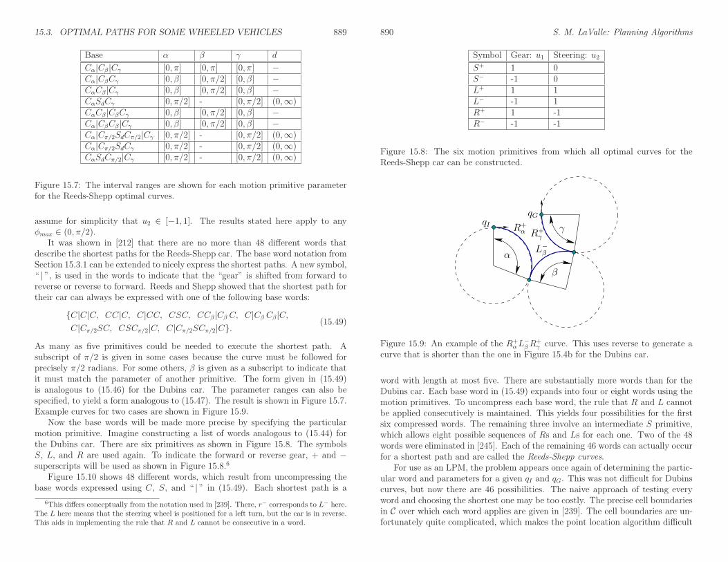
15.3. OPTIMAL PATHS FOR SOME WHEELED VEHICLES 889
Base α β γ d
Cα|Cβ|Cγ [0, π] [0, π] [0, π] −Cα|CβCγ [0, β] [0, π/2] [0, β] −CαCβ|Cγ [0, β] [0, π/2] [0, β] −CαSdCγ [0, π/2] - [0, π/2] (0,∞)CαCβ|CβCγ [0, β] [0, π/2] [0, β] −Cα|CβCβ|Cγ [0, β] [0, π/2] [0, β] −Cα|Cπ/2SdCπ/2|Cγ [0, π/2] - [0, π/2] (0,∞)Cα|Cπ/2SdCγ [0, π/2] - [0, π/2] (0,∞)CαSdCπ/2|Cγ [0, π/2] - [0, π/2] (0,∞)
Figure 15.7: The interval ranges are shown for each motion primitive parameterfor the Reeds-Shepp optimal curves.
assume for simplicity that u2 ∈ [−1, 1]. The results stated here apply to anyφmax ∈ (0, π/2).
It was shown in [212] that there are no more than 48 different words thatdescribe the shortest paths for the Reeds-Shepp car. The base word notation fromSection 15.3.1 can be extended to nicely express the shortest paths. A new symbol,“ | ”, is used in the words to indicate that the “gear” is shifted from forward toreverse or reverse to forward. Reeds and Shepp showed that the shortest path fortheir car can always be expressed with one of the following base words:
{C|C|C, CC|C, C|CC, CSC, CCβ|Cβ C, C|Cβ Cβ|C,C|Cπ/2SC, CSCπ/2|C, C|Cπ/2SCπ/2|C}.
(15.49)
As many as five primitives could be needed to execute the shortest path. Asubscript of π/2 is given in some cases because the curve must be followed forprecisely π/2 radians. For some others, β is given as a subscript to indicate thatit must match the parameter of another primitive. The form given in (15.49)is analogous to (15.46) for the Dubins car. The parameter ranges can also bespecified, to yield a form analogous to (15.47). The result is shown in Figure 15.7.Example curves for two cases are shown in Figure 15.9.
Now the base words will be made more precise by specifying the particularmotion primitive. Imagine constructing a list of words analogous to (15.44) forthe Dubins car. There are six primitives as shown in Figure 15.8. The symbolsS, L, and R are used again. To indicate the forward or reverse gear, + and −superscripts will be used as shown in Figure 15.8.6
Figure 15.10 shows 48 different words, which result from uncompressing thebase words expressed using C, S, and “ | ” in (15.49). Each shortest path is a
6This differs conceptually from the notation used in [239]. There, r− corresponds to L− here.The L here means that the steering wheel is positioned for a left turn, but the car is in reverse.This aids in implementing the rule that R and L cannot be consecutive in a word.
890 S. M. LaValle: Planning Algorithms
Symbol Gear: u1 Steering: u2
S+ 1 0S− -1 0L+ 1 1L− -1 1R+ 1 -1R− -1 -1
Figure 15.8: The six motion primitives from which all optimal curves for theReeds-Shepp car can be constructed.
α
γ
qGqI
β
R+α R+
γ
L−
β
Figure 15.9: An example of the R+αL
−βR
+γ curve. This uses reverse to generate a
curve that is shorter than the one in Figure 15.4b for the Dubins car.
word with length at most five. There are substantially more words than for theDubins car. Each base word in (15.49) expands into four or eight words using themotion primitives. To uncompress each base word, the rule that R and L cannotbe applied consecutively is maintained. This yields four possibilities for the firstsix compressed words. The remaining three involve an intermediate S primitive,which allows eight possible sequences of Rs and Ls for each one. Two of the 48words were eliminated in [245]. Each of the remaining 46 words can actually occurfor a shortest path and are called the Reeds-Shepp curves.
For use as an LPM, the problem appears once again of determining the partic-ular word and parameters for a given qI and qG. This was not difficult for Dubinscurves, but now there are 46 possibilities. The naive approach of testing everyword and choosing the shortest one may be too costly. The precise cell boundariesin C over which each word applies are given in [239]. The cell boundaries are un-fortunately quite complicated, which makes the point location algorithm difficult

15.3. OPTIMAL PATHS FOR SOME WHEELED VEHICLES 891
Base word Sequences of motion primitivesC|C|C (L+R−L+)(L−R+L−)(R+L−R+)(R−L+R−)CC|C (L+R+L−)(L−R−L+)(R+L+R−)(R−L−R+)C|CC (L+R−L−)(L−R+L+)(R+L−R−)(R−L+R+)CSC (L+S+L+)(L−S−L−)(R+S+R+)(R−S−R−)
(L+S+R+)(L−S−R−)(R+S+L+)(R−S−L−)CCβ|Cβ C (L+R+
β L−βR
−)(L−R−β L
+βR
+)(R+L+βR
−β L
−)(R−L−βR
+β L
+)
C|Cβ Cβ|C (L+R−β L
−βR
+)(L−R+β L
+βR
−)(R+L−βR
−β L
+)(R−L+βR
+β L
−)
C|Cπ/2SC (L+R−π/2S
−R−)(L−R+π/2S
+R+)(R+L−π/2S
−L−)(R−L+π/2S
+L+)
(L+R−π/2S
−L−)(L−R+π/2S
+L+) (R+L−π/2S
−R−)(R−L+π/2S
+R+)
CSCπ/2|C (L+S+L+π/2R
−)(L−S−L−π/2R
+)(R+S+R+π/2L
−)(R−S−R−π/2L
+)
(R+S+L+π/2R
−)(R−S−L−π/2R
+)(L+S+R+π/2L
−)(L−S−R−π/2L
+)
C|Cπ/2SCπ/2|C (L+R−π/2S
−L−π/2R
+)(L−R+π/2S
+L+π/2R
−)
(R+L−π/2S
−R−π/2L
+)(R−L+π/2S
+R+π/2L
−)
Figure 15.10: The 48 curves of Reeds and Shepp. Sussmann and Tang [245]showed that (L−R+L−) and (R−L+R−), which appear in the first row, can beeliminated. Hence, only 46 words are needed to describe the shortest paths.
to implement. A simple way to prune away many words from consideration isto use intervals of validity for θ. For some values of θ, certain compressed wordsare impossible as shortest paths. A convenient table of words that become activeover ranges of θ is given in [239]. Once again, the length of the shortest path canserve as a distance function in sampling-based planning algorithms. The resultingReeds-Shepp metric is continuous because the Reeds-Shepp car is STLC, whichwill be established in Section 15.4.
15.3.3 Balkcom-Mason Curves
In recent years, two more families of optimal curves have been determined [18, 67].Recall the differential-drive system from Section 13.1.2, which appears in manymobile robot systems. In many ways, it appears that the differential drive isa special case of the simple car. The expression of the system given in (13.17)can be made to appear identical to the Reeds-Shepp car system in (15.48). Forexample, letting r = 1 and L = 1 makes them equivalent by assigning uω = u1 anduψ = u1u2. Consider the distance traveled by a point attached to the center of thedifferential-drive axle using (15.42). Minimizing this distance for any qI and qG istrivial, as shown in Figure 13.4 of Section 13.1.2. The center point can be made totravel in a straight line in W = R
2. This would be possible for the Reeds-Sheppcar if ρmin = 0, which implies that φmax = π/2. It therefore appeared for manyyears that no interesting curves exist for the differential drive.
The problem, however, with measuring the distance traveled by the axle centeris that pure rotations are cost-free. This occurs when the wheels rotate at the
892 S. M. LaValle: Planning Algorithms
Symbol Left wheel: ul Right wheel: ur
⇑ 1 1⇓ -1 -1x -1 1y 1 -1
Figure 15.11: The four motion primitives from which all optimal curves for thedifferential-drive robot can be constructed.
same speed but with opposite angular velocities. The center does not move;however, the time duration, energy expenditure, and wheel rotations that occurare neglected. By incorporating one or more of these into the cost functional, achallenging optimization arises. Balkcom and Mason bounded the speed of thedifferential drive and minimized the total time that it takes to travel from qI toqG. Using (13.16), the action set is defined as U = [−1, 1]× [−1, 1], in which themaximum rotation rate of each wheel is one (an alternative bound can be usedwithout loss of generality). The criterion to optimize is
L(q, u) =
∫ tF
0
√
x(t)2 + y(t)2 + |θ(t)|dt, (15.50)
which takes θ into account, whereas it was neglected in (15.42). This criterion isonce again equivalent to minimizing the time to reach qG. The resulting model willbe referred to as the Balkcom-Mason drive. An alternative criterion is the totalamount of wheel rotation; this leads to an alternative family of optimal curves[67].
It was shown in [18] that only the four motion primitives shown in Figure15.11 are needed to express time-optimal paths for the differential-drive robot.Each primitive corresponds to holding one action variable fixed at its limit foran interval of time. Using the symbols in Figure 15.11 (which were used in [18]),words can be formed that describe the optimal path. It has been shown that theword length is no more than five. Thus, any shortest paths may be expressed as apiecewise-constant action trajectory in which there are no more than five pieces.Every piece corresponds to one of the primitives in Figure 15.11.
It is convenient in the case of the Balkcom-Mason drive to use the same sym-bols for both base words and for precise specification of primitives. Symmetrytransformations will be applied to each base word to yield a family of eight wordsthat precisely specify the sequences of motion primitives. Nine base words describethe shortest paths:
{y, ⇓, ⇓y, y⇓y, ⇑xπ⇓, x⇓y, ⇓yy, x⇓y⇑, ⇑x⇓y⇑}. (15.51)
This is analogous to the compressed forms given in (15.46) and (15.49). Themotions are depicted in Figure 15.12.

15.3. OPTIMAL PATHS FOR SOME WHEELED VEHICLES 893
Figure 15.12: Each of the nine base words is depicted [18]. The last two are onlyvalid for small motions; they are magnified five times and the robot outline is notdrawn.
Base T1 T2 T3 T2 ◦ T1 T3 ◦ T1 T3 ◦ T2 T3 ◦ T2 ◦ T1A. y y y x y x x x
B. ⇓ ⇑ ⇓ ⇓ ⇑ ⇑ ⇓ ⇑
C. ⇓y ⇑y y⇓ ⇓x y⇑ ⇑x x⇓ x⇑
D. y⇓y y⇑y y⇓y x⇓x y⇑y x⇑x x⇓x x⇑x
E. ⇑xπ⇓ ⇓xπ⇑ ⇓xπ⇑ ⇑yπ⇓ ⇑xπ⇓ ⇓yπ⇑ ⇓yπ⇑ ⇑yπ⇓
F. x⇓y x⇑y y⇓x y⇓x y⇑x y⇑x x⇓y x⇑y
G. ⇓y⇑ ⇑y⇓ ⇑y⇓ ⇓x⇑ ⇓y⇑ ⇑x⇓ ⇑x⇓ ⇓x⇑
H. x⇓y⇑ x⇑y⇓ ⇑y⇓x y⇓x⇑ ⇓y⇑x y⇑x⇓ ⇑x⇓y ⇓x⇑y
I. ⇑x⇓y⇑ ⇓x⇑y⇓ ⇑y⇓x⇑ ⇑y⇓x⇑ ⇓y⇑x⇓ ⇓y⇑x⇓ ⇑x⇓y⇑ ⇓x⇑y⇓
Figure 15.13: The 40 optimal curve types for the differential-drive robot, sortedby symmetry class [18].
894 S. M. LaValle: Planning Algorithms
Figure 15.14: A slice of the optimal curves is shown for qI = (x, y, π4) and qG =
(0, 0, 0) [18]. Level sets of the optimal cost-to-goG∗ are displayed. The coordinatescorrespond to a differential drive with r = L = 1 in (13.16).
Figure 15.13 shows 40 distinct Balkcom-Mason curves that result from apply-ing symmetry transformations to the base words of (15.51). There are 72 entriesin Figure 15.13, but many are identical. The transformation T1 indicates thatthe directions of ⇑ and ⇓ are flipped from the base word. The transformation T2reverses the order of the motion primitives. The transformation T3 flips the direc-tions of x and y. The transformations commute, and there are seven possibleways to combine them, which contributes to a row of Figure 15.13.
To construct an LPM or distance function, the same issues arise as for theReeds-Shepp and Dubins cars. Rather than testing all 40 words to find the shortestpath, simple tests can be defined over which a particular word becomes active[18]. A slice of the precise cell decomposition and the resulting optimal cost-to-go(which can be called the Balkcom-Mason metric) are shown in Figure 15.14.
15.4 Nonholonomic System Theory
This section gives some precision to the term nonholonomic, which was usedloosely in Chapters 13 and 14. Furthermore, small-time controllability (STLC),which was defined in Section 15.1.3, is addressed. The presentation given herebarely scratches the surface of this subject, which involves deep mathematicalprinciples from differential geometry, algebra, control theory, and mechanics. The

15.4. NONHOLONOMIC SYSTEM THEORY 895
intention is to entice the reader to pursue further study of these topics; see thesuggested literature at the end of the chapter.
15.4.1 Control-Affine Systems
Nonholonomic system theory is restricted to a special class of nonlinear systems.The techniques of Section 15.4 utilize ideas from linear algebra. The main conceptswill be formulated in terms of linear combinations of vector fields on a smoothmanifold X. Therefore, the formulation is restricted to control-affine systems,which were briefly introduced in Section 13.2.3. For these systems, x = f(x, u) isof the form
x = h0(x) +m∑
i=1
hi(x)ui, (15.52)
in which each hi is a vector field on X.
The vector fields are expressed using a coordinate neighborhood of X. Usually,m < n, in which n is the dimension of X. Unless otherwise stated, assume thatU = R
m. In some cases, U may be restricted.
Each action variable ui ∈ R can be imagined as a coefficient that determineshow much of hi(x) is blended into the result x. The drift term h0(x) alwaysremains and is often such a nuisance that the driftless case will be the main focus.This means that h0(x) = 0 for all x ∈ X, which yields
x =m∑
i=1
hi(x)ui. (15.53)
The driftless case will be used throughout most of this section. The set h1, . . .,hm, is referred to as the system vector fields. It is essential that U contains atleast an open set that contains the origin of Rm. If the origin is not contained inU , then the system is no longer driftless.7
Control-affine systems arise in many mechanical systems. Velocity constraintson the C-space frequently are of the Pfaffian form (13.5). In Section 13.1.1, it wasexplained that under such constraints, a configuration transition equation (13.6)can be derived that is linear if q is fixed. This is precisely the driftless form (15.53)using X = C. Most of the models in Section 13.1.2 can be expressed in this form.The Pfaffian constraints on configuration are often called kinematic constraintsbecause they arise due to the kinematics of bodies in contact, such as a wheelrolling. The more general case of (15.52) for a phase space X arises from dynamicconstraints that are obtained from Euler-Lagrange equation (13.118) or Hamilton’sequations (13.198) in the formulation of the mechanics. These constraints captureconservation laws, and the drift term usually appears due to momentum.
7Actually, if the convex hull of U contains an open set that contains the origin, then a driftlesssystem can be simulated by rapid switching.
896 S. M. LaValle: Planning Algorithms
Example 15.5 (A Simplified Model for Differential Drives and Cars) Boththe simple-car and the differential-drive models of Section 13.1.2 can be expressedin the form (15.53) after making simplifications. The simplified model, (15.48),can be adapted to conveniently express versions of both of them by using differentrestrictions to define U . The third equation of (15.48) can be reduced to θ = u2without affecting the set of velocities that can be achieved. To conform to (15.53),the equations can then be written in a linear-algebra form as
xy
θ
=
cos θsin θ0
u1 +
001
u2. (15.54)
This makes it clear that there are two system vector fields, which can be combinedby selecting the scalar values u1 and u2. One vector field allows pure translation,and the other allows pure rotation. Without restrictions on U , this system be-haves like a differential drive because the simple car cannot execute pure rotation.Simulating the simple car with (15.54) requires restrictions on U (such as requir-ing that u1 be 1 or −1, as in Section 15.3.2). This is equivalent to the unicyclefrom Figure 13.5 and (13.18).
Note that (15.54) can equivalently be expressed as
xy
θ
=
cos θ 0sin θ 00 1
(
u1u2
)
(15.55)
by organizing the vector fields into a matrix. �
In (15.54), the vector fields were written as column vectors that combine lin-early using action variables. This suggested that control-affine systems can bealternatively expressed using matrix multiplication in (15.55). In general, thevector fields can be organized into an n×m matrix as
H(x) =[
h1(x) h2(x) · · · hm(x)]
. (15.56)
In the driftless case, this yields
x = H(x) u (15.57)
as an equivalent way to express (15.53)It is sometimes convenient to work with Pfaffian constraints,
g1(x)x1 + g2(x)x2 + · · ·+ gn(x)xn = 0, (15.58)
instead of a state transition equation. As indicated in Section 13.1.1, a set of kindependent Pfaffian constraints can be converted into a state transition equation

15.4. NONHOLONOMIC SYSTEM THEORY 897
with m = (n − k) action variables. The resulting state transition equation isa driftless control-affine system. Thus, Pfaffian constraints provide a dual wayof specifying driftless control-affine systems. The k Pfaffian constraints can beexpressed in matrix form as
G(x) x = 0, (15.59)
which is the dual of (15.57), and G(x) is a k × n matrix formed from the gicoefficients of each Pfaffian constraint. Systems with drift can be expressed in aPfaffian-like form by constraints
g0(x) + g1(x)x1 + g2(x)x2 + · · ·+ gn(x)xn = 0. (15.60)
15.4.2 Determining Whether a System Is Nonholonomic
The use of linear algebra in Section 15.4.1 suggests further development of alge-braic concepts. This section briefly introduces concepts that resemble ordinarylinear algebra but apply to linear combinations of vector fields. This providesthe concepts and tools needed to characterize important system properties in theremainder of this section. This will enable the assessment of whether a system isnonholonomic and also whether it is STLC. Many of the constructions are namedafter Sophus Lie (pronounced “lee”), a mathematician who in the nineteenth cen-tury contributed many ideas to algebra and geometry that happen to be relevant inthe study of nonholonomic systems (although that application came much later).
Completely integrable or nonholonomic?
Every control-affine system must be one or the other (not both) of the following:
1. Completely integrable: This means that the Pfaffian form (15.59) can beobtained by differentiating k equations of the form fi(x) = 0 with respectto time. This case was interpreted as being trapped on a surface in Section13.1.3. An example of being trapped on a circle in R
2 was given in (13.22).
2. Nonholonomic: This means that the system is not completely integrable.In this case, it might even be possible to reach all of X, even if the numberof action variables m is much smaller than n, the dimension of X.
In this context, the term holonomic is synonymous with completely integrable,and nonintegrable is synonymous with nonholonomic. The term nonholonomic issometimes applied to non-Pfaffian constraints [159]; however, this will be avoidedhere, in accordance with mechanics literature [34].
The notion of integrability used here is quite different from that required for(14.1). In that case, the state transition equation needed to be integrable to obtainintegral curves from any initial state. This was required for all systems consideredin this book. By contrast, complete integrability implies that the system can be
898 S. M. LaValle: Planning Algorithms
expressed without even using derivatives. This means that all integral curves caneventually be characterized by constraints that do not involve derivatives.
To help understand complete integrability, the notion of an integral curve willbe generalized from one to m dimensions. A manifoldM ⊆ X is called an integralmanifold of a set of Pfaffian constraints if at every x ∈ M , all vectors in thetangent space Tx(M) satisfy the constraints. For a set of completely integrablePfaffian constraints, a partition of X into integral manifolds can be obtained bydefining maximal integral manifolds from every x ∈ X. The resulting partition iscalled a foliation, and the maximal integral manifolds are called leaves [229].
Example 15.6 (A Foliation with Spherical Leaves) As an example, sup-pose X = R
n and consider the Pfaffian constraint
x1x1 + x2x2 + · · · xnxn = 0. (15.61)
This is completely integrable because it can be obtained by differentiating theequation of a sphere,
x21 + x22 + · · · x2n − r2 = 0, (15.62)
with respect to time (r is a constant). The particular sphere that is obtainedvia integration depends on an initial state. The foliation is the collection of allconcentric spheres that are centered at the origin. For example, if X = R
3, then amaximal integral manifold arises for each point of the form (0, 0, r). In each case, itis a sphere of radius r. The foliation is generated by selecting every r ∈ [0,∞). �
The task in this section is to determine whether a system is completely inte-grable. Imagine someone is playing a game with you. You are given an control-affine system and asked to determine whether it is completely integrable. Theperson playing the game with you can start with equations of the form hi(x) = 0and differentiate them to obtain Pfaffian constraints. These can then be convertedinto the parametric form to obtain the state transition equation (15.53). It is easyto construct challenging problems; however, it is very hard to solve them. Theconcepts in this section can be used to determine only whether it is possible towin such a game. The main tool will be the Frobenius theorem, which concludeswhether a system is completely integrable. Unfortunately, the conclusion is ob-tained without producing the integrated constraints hi(x) = 0. Therefore, it isimportant to keep in mind that “integrability” does not mean that you can inte-grate it to obtain a nice form. This is a challenging problem of reverse engineering.On the other hand, it is easy to go in the other direction by differentiating theconstraints to make a challenging game for someone else to play.

15.4. NONHOLONOMIC SYSTEM THEORY 899
Distributions
A distribution8 expresses a set of vector fields on a smooth manifold. Suppose thata driftless control-affine system (15.53) is given. Recall the vector space definitionfrom Section 8.3.1 or from linear algebra. Also recall that a state transitionequation can be interpreted as a vector field if the actions are fixed and as avector space if the state is instead fixed. For U = R
m and a fixed x ∈ X, the statetransition equation defines a vector space in which each hi evaluated at x is abasis vector and each ui is a coefficient. For example, in (15.54), the vector fieldsh1 and h2 evaluated at q = (0, 0, 0) become [1 0 0]T and [0 0 1]T , respectively.These serve as the basis vectors. By selecting values of u ∈ R
2, a 2D vector spaceresults. Any vector of the form [a 0 b]T can be represented by setting u1 = a andu2 = b. More generally, let △(x) denote the vector space obtained in this way forany x ∈ X.
The dimension of a vector space is the number of independent basis vectors.Therefore, the dimension of△(x) is the rank of H(x) from (15.56) when evaluatedat the particular x ∈ X. Now consider defining △(x) for every x ∈ X. This yieldsa parameterized family of vector spaces, one for each x ∈ X. The result couldjust as well be interpreted as a parameterized family of vector fields. For example,consider actions for i from 1 to m of the form ui = 1 and uj = 0 for all i 6= j. Ifthe action is held constant over all x ∈ X, then it selects a single vector field hifrom the collection of m vector fields:
x = hi(x). (15.63)
Using constant actions, an m-dimensional vector space can be defined in whicheach vector field hi is a basis vector (assuming the hi are linearly independent),and the ui ∈ R are the coefficients:
u1h1(x) + u2h2(x) + · · ·+ umhm(x). (15.64)
This idea can be generalized to allow the ui to vary over X. Thus, rather thanhaving u constant, it can be interpreted as a feedback plan π : X → U , in whichthe action at x is given by u = π(x). The set of all vector fields that can beobtained as
π1(x)h1(x) + π2(x)h2(x) + · · ·+ πm(x)hm(x) (15.65)
is called the distribution of the set {h1, . . . , hm} of vector fields and is denoted as△. If △ is obtained from an control-affine system, then △ is called the systemdistribution. The resulting set of vector fields is not quite a vector space becausethe nonzero coefficients πi do not necessarily have a multiplicative inverse. Thisis required for the coefficients of a vector field and was satisfied by using R in thecase of constant actions. A distribution is instead considered algebraically as a
8This distribution has nothing to do with probability theory. It is just an unfortunate coin-cidence of terminology.
900 S. M. LaValle: Planning Algorithms
X x
Tx(X)
T (X)
△△(x)
Figure 15.15: The distribution △ can be imagined as a slice of the tangent bundleT (X). It restricts the tangent space at every x ∈ X.
module [127]. In most circumstances, it is helpful to imagine it as a vector space(just do not try to invert the coefficients!). Since a distribution is almost a vectorspace, the span notation from linear algebra is often used to define it:
△ = span{h1, h2, . . . , hm}. (15.66)
Furthermore, it is actually a vector space with respect to constant actions u ∈ Rm.
Note that for each fixed x ∈ X, the vector space △(x) is obtained, as definedearlier. A vector field f is said to belong to a distribution △ if it can be expressedusing (15.65). If for all x ∈ X, the dimension of △(x) is m, then △ is called anonsingular distribution (or regular distribution). Otherwise,△ is called a singulardistribution, and the points x ∈ X for which the dimension of △(x) is less than mare called singular points. If the dimension of △(x) is a constant c over all x ∈ X,then c is called the dimension of the distribution and is denoted by dim(△). Ifthe vector fields are smooth, and if π is restricted to be smooth, then a smoothdistribution is obtained, which is a subset of the original distribution.
As depicted in Figure 15.15, a nice interpretation of the distribution can begiven in terms of the tangent bundle of a smooth manifold. The tangent bundlewas defined for X = R
n in (8.9) and generalizes to any smooth manifold X toobtain
T (X) =⋃
x∈X
Tx(X). (15.67)
The tangent bundle is a 2n-dimensional manifold in which n is the dimension ofX.A phase space for which x = (q, q) is actually T (C). In the current setting, eachelement of T (X) yields a state and a velocity, (x, x). Which pairs are possible fora driftless control-affine system? Each △(x) indicates the set of possible x valuesfor a fixed x. The point x is sometimes called the base and △(x) is called the fiberover x in T (X). The distribution △ simply specifies a subset of Tx(X) for everyx ∈ X. For a vector field f to belong to △, it must satisfy f(x) ∈ △(x) for all

15.4. NONHOLONOMIC SYSTEM THEORY 901
x ∈ X. This is just a restriction to a subset of T (X). If m = n and the systemvector fields are independent, then any vector field is allowed. In this case, △includes any vector field that can be constructed from the vectors in T (X).
Example 15.7 (The Distribution for the Differential Drive) The systemin (15.54) yields a two-dimensional distribution:
△ = span{[cos θ sin θ 0]T , [0 0 1]T}. (15.68)
The distribution is nonsingular because for any (x, y, θ) in the coordinate neigh-borhood, the resulting vector space △(x, y, θ) is two-dimensional. �
Example 15.8 (A Singular Distribution) Consider the following system,which is given in [130]:
x1x2x3
= h1(x)u1 + h2(x)u2 + h3(x)u3
=
x11 + x3
1
u1 +
x1x2(1 + x3)x2
x2
u2 +
x1x10
u3.
(15.69)
The distribution is△ = span{h1, h2, h3}. (15.70)
The first issue is that for any x ∈ R3, h2(x) = h1(x)x2, which implies that the
vector fields are linearly dependent over all of R3. Hence, this distribution is
singular because m = 3 and the dimension of ∆(x) is 2 if x1 6= 0. If x1 = 0, thenthe dimension of ∆(x) drops to 1. The dimension of △ is not defined because thedimension of ∆(x) depends on x. �
A distribution can alternatively be defined directly from Pfaffian constraints.Each gi(x) = 0 is called an annihilator because enforcing the constraint eliminatesmany vector fields from consideration. At each x ∈ X, △(x) is defined as theset of all velocity vectors that satisfy all k Pfaffian constraints. The constraintsthemselves can be used to form a codistribution, which is a kind of dual to thedistribution. The codistribution can be interpreted as a vector space in whicheach constraint is a basis vector. Constraints can be added together or multipliedby any c ∈ R, and there is no effect on the resulting distribution of allowablevector fields.
Lie brackets
The key to establishing whether a system is nonholonomic is to construct motionsthat combine the effects of two action variables, which may produce motions
902 S. M. LaValle: Planning Algorithms
q(0) q(∆t)
q(2∆t)
x
y
q(2∆t)
q(4∆t)
q(3∆t)
y
x
(a) (b)
Figure 15.16: (a) The effect of the first two primitives. (b) The effect of the lasttwo primitives.
in a direction that seems impossible from the system distribution. To motivatethe coming ideas, consider the differential-drive model from (15.54). Apply thefollowing piecewise-constant action trajectory over the interval [0, 4∆t]:
u(t) =
(1, 0) for t ∈ [0,∆t)(0, 1) for t ∈ [∆t, 2∆t)(−1, 0) for t ∈ [2∆t, 3∆t)(0,−1) for t ∈ [3∆t, 4∆t] .
(15.71)
The action trajectory is a sequence of four motion primitives: 1) translate forward,2) rotate forward, 3) translate backward, and 4) rotate backward.
The result of all four motion primitives in succession from qI = (0, 0, 0) isshown in Figure 15.16. It is fun to try this at home with an axle and two wheels(Tinkertoys work well, for example). The result is that the differential drive movessideways!9 From the transition equation (15.54) such motions appear impossible.This is a beautiful property of nonlinear systems. The state may wiggle its way indirections that do not seem possible. A more familiar example is parallel parking acar. It is known that a car cannot directly move sideways; however, some wigglingmotions can be performed to move it sideways into a tight parking space. Theactions we perform while parking resemble the primitives in (15.71).
Algebraically, the motions of (15.71) appear to be checking for commutativity.Recall from Section 4.2.1 that a group G is called commutative (or Abelian) ifab = ba for any a, b ∈ G. A commutator is a group element of the form aba−1b−1.
9It also moves slightly forward; however, this can be eliminated by either lengthening thetime of the third primitive or by considering the limit as ∆ approaches zero.

15.4. NONHOLONOMIC SYSTEM THEORY 903
−g
−f
g
fx(∆t)
x(2∆t)
x(0)
x(3∆t)
Figure 15.17: The velocity obtained by the Lie bracket can be approximated bya sequence of four motion primitives.
If the group is commutative, then aba−1b−1 = e (the identity element) for anya, b ∈ G. If a nonidentity element of G is produced by the commutator, then thegroup is not commutative. Similarly, if the trajectory arising from (15.71) does notform a loop (by returning to the starting point), then the motion primitives do notcommute. Therefore, a sequence of motion primitives in (15.71) will be referred toas the commutator motion. It will turn out that if the commutator motion cannotproduce any velocities not allowed by the system distribution, then the system iscompletely integrable. This means that if we are trapped on a surface, then it isimpossible to leave the surface by using commutator motions.
Now generalize the differential drive to any driftless control-affine system thathas two action variables:
x = f(x)u1 + g(x)u2. (15.72)
Using the notation of (15.53), the vector fields would be h1 and h2; however, fand g are chosen here to allow subscripts to denote the components of the vectorfield in the coming explanation.
Suppose that the commutator motion (15.71) is applied to (15.72) as shown inFigure 15.17. Determining the resulting motion requires some general computa-tions, as opposed to the simple geometric arguments that could be made for thedifferential drive. If would be convenient to have an expression for the velocityobtained in the limit as ∆t approaches zero. This can be obtained by using Tay-lor series arguments. These are simplified by the fact that the action history ispiecewise constant.
The coming derivation will require an expression for x under the application ofa constant action. For each action, a vector field of the form x = h(x) is obtained.Upon differentiation, this yields
x =dh
dt=∂h
∂x
dx
dt=∂h
dxx =
∂h
dxh(x). (15.73)
This follows from the chain rule because h is a function of x, which itself is a
904 S. M. LaValle: Planning Algorithms
function of t. The derivative ∂h/∂x is actually an n× n Jacobian matrix, whichis multiplied by the vector x. To further clarify (15.73), each component can beexpressed as
xi =d
dthi(x(t)) =
n∑
j=1
∂hi∂xj
hj. (15.74)
Now the state trajectory under the application of (15.71) will be determinedusing the Taylor series, which was given in (14.17). The state trajectory thatresults from the first motion primitive u = (1, 0) can be expressed as
x(∆t) = x(0) + ∆t x(0) + 12(∆t)2 x(0) + · · ·
= x(0) + ∆t f(x(0)) +1
2(∆t)2
∂f
∂x
∣
∣
∣
x(0)f(x(0)) + · · · ,
(15.75)
which makes use of (15.73) in the second line. The Taylor series expansion for thesecond primitive is
x(2∆t) = x(∆t) + ∆t g(x(∆t)) +1
2(∆t)2
∂g
∂x
∣
∣
∣
x(∆t)g(x(∆t)) + · · · . (15.76)
An expression for g(x(∆t)) can be obtained by using the Taylor series expansionin (15.75) to express x(∆t). The first terms after substitution and simplificationare
x(2∆t) = x(0) + ∆t (f + g) + (∆t)2(
1
2
∂f
∂xf +
∂g
∂xf +
1
2
∂g
∂xg
)
+ · · · . (15.77)
To simplify the expression, the evaluation at x(0) has been dropped from everyoccurrence of f and g and their derivatives.
The idea of substituting previous Taylor series expansions as they are neededcan be repeated for the remaining two motion primitives. The Taylor series ex-pansion for the result after the third primitive is
x(3∆t) = x(0) + ∆t g + (∆t)2(
∂g
∂xf − ∂f
∂xg +
1
2
∂g
∂xg
)
+ · · · . (15.78)
Finally, the Taylor series expansion after all four primitives have been applied is
x(4∆t) = x(0) + (∆t)2(
∂g
∂xf − ∂f
∂xg
)
+ · · · . (15.79)
Taking the limit yields
lim∆t→0
x(4∆t)− x(0)(∆t)2
=∂g
∂xf − ∂f
∂xg, (15.80)

15.4. NONHOLONOMIC SYSTEM THEORY 905
which is called the Lie bracket of f and g and is denoted by [f, g]. Similar to(15.74), the ith component can be expressed as
[f, g]i =n∑
j=1
(
fj∂gi∂xj− gj
∂fi∂xj
)
. (15.81)
The Lie bracket is an important operation in many subjects, and is related to thePoisson and Jacobi brackets that arise in physics and mathematics.
Example 15.9 (Lie Bracket for the Differential Drive) The Lie bracket shouldindicate that sideways motions are possible for the differential drive. Consider tak-ing the Lie bracket of the two vector fields used in (15.54). Let f = [cos θ sin θ 0]T
and g = [0 0 1]T . Rename h1 and h2 to f and g to allow subscripts to denotethe components of a vector field.
By applying (15.81), the Lie bracket [f, g] is
[f, g]1 = f1∂g1∂x− g1
∂f1∂x
+ f2∂g1∂y− g2
∂f1∂y
+ f3∂g1∂θ− g3
∂f1∂θ
= sin θ
[f, g]2 = f1∂g2∂x− g1
∂f2∂x
+ f2∂g2∂y− g2
∂f2∂y
+ f3∂g2∂θ− g3
∂f2∂θ
= − cos θ
[f, g]3 = f1∂g3∂x− g1
∂f3∂x
+ f2∂g3∂y− g2
∂f3∂y
+ f3∂g3∂θ− g3
∂f3∂θ
= 0.
(15.82)
The resulting vector field is [f, g] = [sin θ − cos θ 0]T , which indicates the side-ways motion, as desired. When evaluated at q = (0, 0, 0), the vector [0 − 1 0]T
is obtained. This means that performing short commutator motions wiggles thedifferential drive sideways in the −y direction, which we already knew from Figure15.16. �
Example 15.10 (Lie Bracket of Linear Vector Fields) Suppose that eachvector field is a linear function of x. The n × n Jacobians ∂f/∂x and ∂g/∂x areconstant.
As a simple example, recall the nonholonomic integrator (13.43). In the linear-algebra form, the system is
x1x2x3
=
10−x2
u1 +
01x1
u2. (15.83)
Let f = h1 and g = h2. The Jacobian matrices are
∂f
∂x=
0 0 00 0 00 −1 0
and∂g
∂x=
0 0 00 0 01 0 0
. (15.84)
906 S. M. LaValle: Planning Algorithms
Using (15.80),
∂g
∂xf − ∂f
∂xg =
0 0 00 0 01 0 0
10−x2
−
0 0 00 0 00 −1 0
01−x1
=
002
. (15.85)
This result can be verified using (15.81).�
The Frobenius Theorem
The Lie bracket is the only tool needed to determine whether a system is com-pletely integrable (holonomic) or nonholonomic (not integrable). Suppose that asystem of the form (15.53) is given. Using the m system vector fields h1, . . ., hmthere are (m2 ) Lie brackets of the form [hi, hj] for i < j that can be formed. Adistribution △ is called involutive [42] if for each of these brackets there exist mcoefficients ck ∈ R such that
[hi, hj ] =m∑
k=1
ckhk. (15.86)
In other words, every Lie bracket can be expressed as a linear combination of thesystem vector fields, and therefore it already belongs to △. The Lie brackets areunable to escape △ and generate new directions of motion. We did not need toconsider all n2 possible Lie brackets of the system vector fields because it turnsout that [hi, hj] = −[hj, hi] and consequently [hi, hi] = 0. Therefore, the definitionof involutive is not altered by looking only at the (m2 ) pairs.
If the system is smooth and the distribution is nonsingular, then the Frobeniustheorem immediately characterizes integrability:
A system is completely integrable if and only if it is involutive.
Proofs of the Frobenius theorem appear in numerous differential geometry andcontrol theory books [42, 51, 130, 221]. There also exist versions that do notrequire the distribution to be nonsingular.
Determining integrability involves performing Lie brackets and determiningwhether (15.86) is satisfied. The search for the coefficients can luckily be avoidedby using linear algebra tests for linear independence. The n × m matrix H(x),which was defined in (15.56), can be augmented into an n× (m+1) matrix H ′(x)by adding [hi, hj] as a new column. If the rank of H ′(x) is m + 1 for any pairhi and hj, then it is immediately known that the system is nonholonomic. If therank of H ′(x) is m for all Lie brackets, then the system is completely integrable.Driftless linear systems, which are expressed as x = Bu for a fixed matrix B, arecompletely integrable because all Lie brackets are zero.

15.4. NONHOLONOMIC SYSTEM THEORY 907
Example 15.11 (The Differential Drive Is Nonholonomic) For the dif-ferential drive model in (15.54), the Lie bracket [f, g] was determined in Example15.9 to be [sin θ − cos θ 0]T . The matrix H ′(q), in which q = (x, y, θ), is
H ′(q) =
cos θ 0 sin θsin θ 0 − cos θ0 1 0
. (15.87)
The rank of H ′(q) is 3 for all q ∈ C (the determinant of H ′(q) is 1). Therefore, bythe Frobenius theorem, the system is nonholonomic. �
Example 15.12 (The Nonholonomic Integrator Is Nonholonomic) Wewould hope that the nonholonomic integrator is nonholonomic. In Example 15.10,the Lie bracket was determined to be [0 0 2]T . The matrix H ′(q) is
H ′(q) =
1 0 00 1 0−x2 x1 2
, (15.88)
which clearly has full rank for all q ∈ C. �
Example 15.13 (Trapped on a Sphere) Suppose that the following systemis given:
x1x2x3
=
x2−x10
u1 +
x30−x1
u2, (15.89)
for which X = R3 and U = R
2. Since the vector fields are linear, the Jacobiansare constant (as in Example 15.10):
∂f
∂x=
0 1 0−1 0 00 0 0
and∂g
∂x=
0 0 10 0 0−1 0 0
. (15.90)
Using (15.80),
∂g
∂xf − ∂f
∂xg =
0 0 10 0 0−1 0 0
x2−x10
−
0 1 0−1 0 00 0 0
x30−x1
=
0x3−x2
. (15.91)
This yields the matrix
H ′(x) =
x2 −x1 0x3 0 −x10 x3 −x2
. (15.92)
908 S. M. LaValle: Planning Algorithms
The determinant is zero for all x ∈ R3, which means that [f, g] is never linearly
independent of f and g. Therefore, the system is completely integrable.10
The system can actually be constructed by differentiating the equation of asphere. Let
f(x) = x21 + x22 + x23 − r2 = 0, (15.93)
and differentiate with respect to time to obtain
x1x1 + x2x2 + x3x3 = 0, (15.94)
which is a Pfaffian constraint. A parametric representation of the set of vectorsthat satisfy (15.94) is given by (15.89). For each (u1, u2) ∈ R
2, (15.89) yieldsa vector that satisfies (15.94). Thus, this was an example of being trapped ona sphere, which we would expect to be completely integrable. It was difficult,however, to suspect this using only (15.89). �
15.4.3 Determining Controllability
Determining complete integrability is the first step toward determining whethera driftless control-affine system is STLC. The Lie bracket attempts to producemotions in directions that do not seem to be allowed by the system distribution.At each q, a velocity not in △(q) may be produced by the Lie bracket. Byworking further with Lie brackets, it is possible to completely characterize all ofthe directions that are possible from each q. So far, the Lie brackets have only beenapplied to the system vector fields h1, . . ., hm. It is possible to proceed further byapplying Lie bracket operations on Lie brackets. For example, [h1, [h1, h2]] can becomputed. This might generate a vector field that is linearly independent of allof the vector fields considered in Section 15.4.2 for the Frobenius theorem. Themain idea in this section is to apply the Lie bracket recursively until no moreindependent vector fields can be found. The result is called the Lie algebra. Ifthe number of independent vector fields obtained in this way is the dimension ofX, then it turns out that the system is STLC.
The Lie algebra
The notion of a Lie algebra is first established in general. Let V be any vectorspace with coefficients in R. In V , the vectors can be added or multiplied byelements of R; however, there is no way to “multiply” two vectors to obtain athird. The Lie algebra introduces a product operation to V . The product iscalled a bracket or Lie bracket (considered here as a generalization of the previousLie bracket) and is denoted by [·, ·] : V × V → V .
10This system is singular at the origin. A variant of the Frobenius theorem given here istechnically needed.

15.4. NONHOLONOMIC SYSTEM THEORY 909
To be a Lie algebra obtained from V , the bracket must satisfy the followingthree axioms:
1. Bilinearity: For any a, b ∈ R and u, v, w ∈ V ,
[au+ bv, w] = a[u, w] + b[v, w]
[u, av + bw] = a[u, w] + b[u, w].(15.95)
2. Skew symmetry: For any u, v ∈ V ,
[u, v] = −[v, u]. (15.96)
This means that the bracket is anti-commutative.
3. Jacobi identity: For any u, v, w ∈ V ,
[[u, v], w] + [[v, w], u] + [[w, u], v] = 0. (15.97)
Note that the bracket is not even associative.
Let L(V ) denote the Lie algebra of V . This is a vector space that includes allelements of V and any new elements that can be obtained via Lie bracket opera-tions. The Lie algebra L(V ) includes every vector that can be obtained from anyfinite number of nested Lie bracket operations. Thus, describing a Lie algebrarequires characterizing all vectors that are obtained under the algebraic closure ofthe bracket operation. Since L(V ) is a vector space, this is accomplished by find-ing a basis of independent vectors of which all elements of L(V ) can be expressedas a linear combination.
Example 15.14 (The Vector Cross Product) Let V be the vector spaceover R3 that is used in vector calculus. The basis elements are often denoted ası, , and k. A bracket for this vector space is simply the cross product
[u, v] = u× v. (15.98)
It can be verified that the required axioms of a Lie bracket are satisfied.One interesting property of the cross product that is exploited often in analytic
geometry is that it produces a vector outside of the span of u and v. For example,let W be the two-dimensional subspace of vectors
W = span{ı, }. (15.99)
The cross product always yields a vector that is a multiple of k, which lies outsideof V if the product is nonzero. This behavior is very similar to constructing vectorfields that lie outside of △ using the Lie bracket in Section 15.4.2. �
910 S. M. LaValle: Planning Algorithms
Example 15.15 (Lie Algebra on Lie Groups) Lie groups are the most im-portant application of the Lie algebra concepts. Recall from Section 4.2.1 thenotion of a matrix group. Important examples throughout this book have beenSO(n) and SE(n). If interpreted as a smooth manifold, these matrix groups areexamples of Lie groups [17]. In general, a Lie group G is both a differentiablemanifold and a group with respect to some operation ◦ if and only if:
1. The product a ◦ b, interpreted as a function from G×G→ G, is smooth.
2. The inverse a−1, interpreted as a function from G to G, is smooth.
The two conditions are needed to prevent the group from destroying the niceproperties that come with the smooth manifold. An important result in the studyof Lie groups is that all compact finite-dimensional Lie groups can be representedas matrix groups.
For any Lie group, a Lie algebra can be defined on a special set of vectorfields. These are defined using the left translation mapping Lg : x 7→ gx. Thevector field formed from the differential of Lg is called a left-invariant vector field.A Lie algebra can be defined on the set of these fields. The Lie bracket definitiondepends on the particular group. For the case of GL(n), the Lie bracket is
[A,B] = AB − BA. (15.100)
In this case, the Lie bracket clearly appears to be a test for commutativity. Ifthe matrices commute with respect to multiplication, then the Lie bracket is zero.The Lie brackets for SO(n) and SE(n) are given in many texts on mechanics andcontrol [51, 221]. The Lie algebra of left-invariant vector fields is an importantstructure in the study of nonlinear systems and mechanics. �
Lie algebra of the system distribution
Now suppose that a set h1, . . ., hm of vector fields is given as a driftless control-affine system, as in (15.53). Its associated distribution△ is interpreted as a vectorspace with coefficients in R, and the Lie bracket operation was given by (15.81).It can be verified that the Lie bracket operation in (15.81) satisfies the requiredaxioms for a Lie algebra.
As observed in Examples 15.9 and 15.10, the Lie bracket may produce vectorfields outside of△. By defining the Lie algebra of△ to be all vector fields that canbe obtained by applying Lie bracket operations, a potentially larger distributionL(△) is obtained. The Lie algebra can be expressed using the span notation byincluding h1, . . ., hm and all independent vector fields generated by Lie brackets.Note that no more than n independent vector fields can possibly be produced.
Example 15.16 (The Lie Algebra of the Differential Drive) The Lie al-gebra of the differential drive (15.54) is
L(△) = span{[cos θ sin θ 0]T , [0 0 1]T , [sin θ − cos θ 0]T}. (15.101)

15.4. NONHOLONOMIC SYSTEM THEORY 911
This uses the Lie bracket that was computed in (15.82) to obtain a three-dimensionalLie algebra. No further Lie brackets are needed because the maximum number ofindependent vector fields has been already obtained. �
Example 15.17 (A Lie Algebra That Involves Nested Brackets) The pre-vious example was not very interesting because the Lie algebra was generated aftercomputing only one bracket. Suppose that X = R
5 and U = R2. In this case,
there is room to obtain up to three additional, linearly independent vector fields.The dimension of the Lie algebra may be any integer from 2 to 5.
Let the system be
x1x2x3x4x5
=
10x2x3x4
u1 +
01000
u2. (15.102)
This is a chained-form system, which is a concept that becomes important inSection 15.5.2.
The first Lie bracket produces
[h1, h2] = [0 0 − 1 0 0]T . (15.103)
Other vector fields that can be obtained by Lie brackets are
[h1, [h1, h2]] = [0 0 0 1 0]T (15.104)
and[h1, [h1, [h1, h2]]] = [0 0 0 0 1]T . (15.105)
The resulting five vector fields are independent over all x ∈ R5. This includes
h1, h2, and the three obtained from Lie bracket operations. Independence can beestablished by placing them into a 5× 5 matrix,
1 0 0 0 00 1 0 0 0x2 0 −1 0 0x3 0 0 1 0x4 0 0 0 1
, (15.106)
which has full rank for all x ∈ R5. No additional vector fields can possibly be
independent. Therefore, the five-dimensional Lie algebra is
L(△) = span{h1, h2, [h1, h2], [h1, [h1, h2]], [h1, [h1, [h1, h2]]]}. (15.107)
�
912 S. M. LaValle: Planning Algorithms
Philip Hall basis of a Lie algebra
Determining the basis of a Lie algebra may be a long and tedious process. Thecombinations of Lie brackets in Example 15.17 were given; however, it is not knownin advance which ones will produce independent vector fields. Numerous Liebrackets may be needed, including some that are nested, such as [[h1, h2], h3]. Themaximum depth of nested Lie bracket operations is not known a priori. Therefore,a systematic search must be performed (this can in fact be modeled as a discreteplanning problem) by starting with h1, . . ., hm and iteratively generating new,independent vector fields using Lie brackets.
One popular approach is to generate the Philip Hall basis (or P. Hall basis) ofthe Lie algebra L(△). The construction of the basis essentially follows breadth-first search, in which the search depth is defined to be the number of nested levelsof bracket operations. The order (or depth) d of a Lie product is defined recursivelyas follows. For the base case, let d(hi) = 1 for any of the system vector fields. Forany Lie product [φ1, φ2], let
d([φ1, φ2]) = d(φ1) + d(φ2). (15.108)
Thus, the order is just the nesting depth (plus one) of the Lie bracket operations.For example, d([h1, h2]) = 2 and d([h1, [h2, h3]]) = 3.
In addition to standard breadth-first search, pruning should be automaticallyperformed to ensure that the skew symmetry and Jacobi identities are alwaysutilized to eliminate redundancy. A P. Hall basis is a sequence, PH = (φ1, φ2,. . .), of Lie products for which:
1. The system vector fields hi are the first m elements of PH.
2. If d(φi) < d(φj), then i < j.
3. Each [φi, φj] ∈ PH if and only if: a) φi, φj ∈ PH and i < j, and b) eitherφj = hi for some i or φj = [φl, φr] for some φl, φr ∈ PH such that l ≤ i.
It is shown in many algebra books (e.g., [227]) that this procedure results in abasis for the Lie algebra L(△). Various algorithms for computing the basis areevaluated in [86].
Example 15.18 (P. Hall Basis Up to Depth Three) The P. Hall basis sortsthe Lie products into the following sequence, which is obtained up to depth d = 3:
h1, h2, h3,[h1, h2], [h2, h3], [h1, h3],[h1, [h1, h2]], [h1, [h1, h3]], [h2, [h1, h2]], [h2, [h1, h3]],[h2, [h2, h3]], [h3, [h1, h2]], [h3, [h1, h3]], [h3, [h2, h3]] .
So far, the only Lie product eliminated by the Jacobi identity is [h1, [h2, h3]] be-cause
[h1, [h2, h3]] = [h2, [h1, h3]]− [h3, [h1, h2]]. (15.109)

15.4. NONHOLONOMIC SYSTEM THEORY 913
Note that all of the Lie products given here may not be linearly independent vec-tor fields. For a particular system, linear independence tests should be performedto delete any linearly dependent vector fields from the basis. �
When does the sequence PH terminate? Recall that dim(L(△)) can be nogreater than n, because Lx(△) ⊆ Tx(X). In other words, at every state x ∈ X,the number of possible independent velocity vectors is no more than the dimensionof the tangent space at x. Therefore, PH can be terminated once n independentvector fields are obtained because there is no possibility of finding more. Forsome systems, there may be a depth k after which all Lie brackets are zero. Suchsystems are called nilpotent of order k. This occurs, for example, if all componentsof all vector fields are polynomials. If the system is not nilpotent, then achievingtermination may be difficult. It may be the case that dim(L(△)) is strictly lessthan n, but this is usually not known in advance. It is difficult to determinewhether more Lie brackets are needed to increase the dimension or the limit hasalready been reached.
Controllability of driftless systems
The controllability of a driftless control-affine system (15.53) can be characterizedusing the Lie algebra rank condition (or LARC). Recall the definition of STLCfrom Section 15.1.3. Assume that either U = R
m or U at least contains an openset that contains the origin of Rm. The Chow-Rashevskii theorem [34, 51, 221]states:
A driftless control-affine system, (15.53), is small-time locally controllable (STLC)at a point x ∈ X if and only if dim(Lx(△)) = n, the dimension of X.
If the condition holds for every x ∈ X, then the whole system is STLC.Integrability can also be expressed in terms of dim(L(△)). Assume as usual thatm < n. The three cases are:
1. dim(L(△)) = m the system is completely integrable;2. m < dim(L(△)) < n the system is nonholonomic, but not STLC;3. dim(L(△)) = n the system is nonholonomic and STLC.
(15.110)
Example 15.19 (Controllability Examples) The differential drive, nonholo-nomic integrator, and the system from Example 15.17 are all STLC by the Chow-Rashevskii theorem because dim(L(△)) = n. This implies that the state can bechanged in any direction, even though there are differential constraints. The statecan be made to follow arbitrarily close to any smooth curve in X. A methodthat achieves this based on the Lie algebra is given in Section 15.5.1. The factthat these systems are STLC assures the existence of an LPM that satisfies the
914 S. M. LaValle: Planning Algorithms
topological property of Section 14.6.2. �
Handling Control-Affine Systems with Drift
Determining whether a system with drift (15.52), is STLC is substantially moredifficult. Imagine a mechanical system, such as a hovercraft, that is moving ata high speed. Due to momentum, it is impossible from most states to move incertain directions during an arbitrarily small interval of time. One can, however,ask whether a system is STLC from a state x ∈ X for which h0(x) = 0. Fora mechanical system, this usually means that it starts at rest. If a system withdrift is STLC, this intuitively means that it can move in any direction by hoveringaround states that are close to zero velocity for the mechanical system.
The Lie algebra techniques can be extended to determine controllability forsystems with drift; however, the tools needed are far more complicated. SeeChapter 7 of [51] for more complete coverage. Even if dim(L(△)) = n, it does notnecessarily imply that the system is STLC. It does at least imply that the systemis accessible, which motivates the definition given in Section 15.1.3. Thus, the setof achievable velocities still has dimension n; however, motions in all directionsmay not be possible due to drift. To obtain STLC, a sufficient condition is thatthe set of possible values for x contains an open set that contains the origin.
The following example clearly illustrates the main difficultly with establishingwhether a system with drift is STLC.
Example 15.20 (Accessible, Not STLC) The following simple system clearlyillustrates the difficulty caused by drift and was considered in [196]. Let X = R
2,U = R, and the state transition equation be
x1 = u
x2 = x21.(15.111)
This system is clearly not controllable in any sense because x2 cannot be decreased.The vector fields are h0(x) = [0 x21]
T and h1(x) = [1 0]T . The first independentLie bracket is
[h1, [h0, h1]] = [0 − 2]. (15.112)
The two-dimensional Lie algebra is
L(△) = span{h1, [h1, [h0, h1]]}, (15.113)
which implies that the system is accessible. It is not STLC, however, because thebracket [h1, [h0, h1]] was constructed using h0 and was combined in an unfortunateway. This bracket is indicating that changing x2 is possible; however, we alreadyknow that it is not possible to decrease x2. Thus, some of the vector fields obtainedfrom Lie brackets that involve h0 may have directional constraints. �

15.5. STEERING METHODS FOR NONHOLONOMIC SYSTEMS 915
In Example 15.20, [h1, [h0, h1]] was an example of a bad bracket [247] becauseit obstructed controllability. A method of classifying brackets as good or bad hasbeen developed, and there exist theorems that imply whether a system with driftis STLC by satisfying certain conditions on the good and bad brackets. Intuitively,there must be enough good brackets to neutralize the obstructions imposed by thebad brackets [51, 247].
15.5 Steering Methods for Nonholonomic Sys-
tems
This section briefly surveys some methods that solve the BVP for nonholonomicsystems. This can be considered as a motion planning problem under differentialconstraints but in the absence of obstacles. For linear systems, optimal controltechniques can be used, as covered in Section 15.2.2. For mechanical systems thatare fully actuated, standard control techniques such as the acceleration-basedcontrol model in (8.47) can be applied. If a mechanical system is underactuated,then it is likely to be nonholonomic. As observed in Section 15.4, it is possible togenerate motions that appear at first to be prohibited. Suppose that by the Chow-Rashevskii theorem, it is shown that a driftless system is STLC. This indicatesthat it should be possible to design an LPM that successfully connects any pairof initial and goal states. The next challenge is to find an action trajectory uthat actually causes xI to reach xG upon integration in (14.1). Many methodsin Chapter 14 could actually be used, but it is assumed that these would be tooslow. The methods in this section exploit the structure of the system (e.g, itsLie algebra) and the fact that there are no obstacles to more efficiently solve theplanning problem.
15.5.1 Using the P. Hall Basis
The steering method presented in this section is due to Lafferriere and Sussmann[152]. It is assumed here that a driftless control-affine system is given, in whichX is a Lie group, as introduced in Example 15.15. Furthermore, the system isassumed to be STLC. The steering method sketched in this section follows fromthe Lie algebra L(△). The idea is to apply piecewise-constant motion primitivesto move in directions given by the P. Hall basis. If the system is nilpotent, thenthis method reaches the goal state exactly. Otherwise, it leads to an approximatemethod that can be iterated to get arbitrarily close to the goal. Furthermore,some systems are nilpotentizable by using feedback [122].
The main idea is to start with (15.53) and construct an extended system
x =s∑
i=1
bi(x)vi, (15.114)
916 S. M. LaValle: Planning Algorithms
in which each vi is an action variable, and bi is a vector field in PH, the P. Hallbasis. For every i ≤ m, each term of (15.114) is bi(x)vi = hi(x)ui, which comesfrom the original system. For i > m, each bi represents a Lie product in PH, andvi is a fictitious action variable. It is called fictitious because the velocity givenby bi for i > m cannot necessarily be achieved by using a single action variable ofthe system. In general, s may be larger than n because at each x ∈ X a differentsubset of PH may be needed to obtain n independent vectors. Also, includingmore basis elements simplifies some of the coming computations.
Example 15.21 (Extended System for the Nonholonomic Integrator) Theextended system for the nonholonomic integrator (15.83) is
x1x2x3
=
10−x2
v1 +
01x1
v2 +
002
v3. (15.115)
The first two terms correspond to the original system. The last term arises fromthe Lie bracket [h1, h2]. Only one fictitious action variable is needed because thethree P. Hall vector fields are independent at every x ∈ X.
It is straightforward to move this system along a grid-based path in R3. Mo-
tions in the x1 and x2 directions are obtained by applying v1 = u1 and v2 = u2,respectively. To move the system in the x3 direction, the commutator motionin (15.71) should be performed. This corresponds to applying v3. The steeringmethod described in this section yields a generalization of this approach. Higherdegree Lie products can be used, and motion in any direction can be achieved. �
Suppose some xI and xG are given. There are two phases to the steeringmethod:
1. Determine an action trajectory v for the extended system, for which x(0) =xI and x(tF ) = xG for some tF > 0.
2. Convert v into an action trajectory u that eliminates the fictitious variablesand uses the actual m action variables u1, . . . , um.
The first phase is straightforward. For the extended system, any velocity in thetangent space, Tx(X), can be generated. Start with any smooth path τ : [0, 1]→X such that τ(0) = xI and τ(1) = xG. The velocity τ(t) along the path τ is avelocity vector in Tτ(t)(X) that can be expressed as a linear combination of thebi(τ(t)) vectors using linear algebra. The coefficients of this combination are the vivalues. The second phase is much more complicated and will be described shortly.If the system is nilpotent, then u should bring the system precisely from xI to xG.By the way it is constructed, it will also be clear how to refine u to come as closeas desired to the trajectory produced by v.
15.5. STEERING METHODS FOR NONHOLONOMIC SYSTEMS 917
Formal calculations The second phase is solved using formal algebraic com-putations. This means that the particular vector fields, differentiation, manifolds,and so on, can be ignored. The concepts involve pure algebraic manipulation.To avoid confusion with previous definitions, the term formal will be added tomany coming definitions. Recall from Section 4.4.1 the formal definitions of thealgebra of polynomials (e.g., F[x1, . . . , xn]). Let A(y1, . . . , ym) denote the formalnoncommutative algebra11 of polynomials in the variables y1, . . ., ym. The yi hereare treated as symbols and have no other assumed properties (e.g, they are notnecessarily vector fields). When polynomials are multiplied in this algebra, nosimplifications can be made based on commutativity. The algebra can be con-verted into a Lie algebra by defining a Lie bracket. For any two polynomialsp, q ∈ A(y1, . . . , ym), define the formal Lie bracket to be [p, q] = pq − qp. Theformal Lie bracket yields an equivalence relation on the algebra; this results in aformal Lie algebra L(y1, . . . , ym) (there are many equivalent expressions for thesame elements of the algebra when the formal Lie bracket is applied). Nilpotentversions of the formal algebra and formal Lie algebra can be made by forcing allmonomials of degree k + 1 to be zero. Let these be denoted by Ak(y1, . . . , ym)and Lk(y1, . . . , ym), respectively. The P. Hall basis can be applied to obtain abasis of the formal Lie algebra. Example 15.18 actually corresponds to the basisof L3(h1, h2, h3) using formal calculations.
The exponential map The steering problem will be solved by performing cal-culations on Lk(y1, . . . , ym). The formal power series of A(y1, . . . , ym) is the set ofall linear combinations of monomials, including those that have an infinite numberof terms. Similarly, the formal Lie series of L(y1, . . . , ym) can be defined.
The formal exponential map is defined for any p ∈ A(y1, . . . , ym) as
ep = 1 + p+1
2!p2 +
1
3!p3 + · · · . (15.116)
In the nilpotent case, the formal exponential map is defined for any p ∈ Ak(y1, . . . , ym)as
ep =k∑
i=0
pi
i!. (15.117)
The formal series is truncated because all terms with exponents larger than kvanish.
A formal Lie group is constructed as
Gk(y1, . . . , ym) = {ep | p ∈ Lk(y1, . . . , ym)}. (15.118)
If the formal Lie algebra is not nilpotent, then a formal Lie group G(y1, . . . , ym)can be defined as the set of all ep, in which p is represented using a formal Lieseries.
11Intuitively, being an algebra means that polynomials can be added and multiplied; for allof the required axioms, see [127].
918 S. M. LaValle: Planning Algorithms
The following example is taken from [152]:
Example 15.22 (Formal Lie Groups) Suppose that the generators x and yare given. Some elements of the formal Lie group G(x, y) are
ex = I + x+ 12x2 + 1
6x3 + · · · , (15.119)
e[x,y] = I + [x, y] + 12[x, y]2 + · · · , (15.120)
and
ex−y+3[x,y] = I + x− y + 3[x, y] + · · · , (15.121)
in which I is the formal Lie group identity. Some elements of the formal Lie groupG2(x, y) are
ex = I + x+ 12x2, (15.122)
e[x,y] = I + [x, y], (15.123)
and
ex−y+3[x,y] = I + x− y + 3[x, y] + 12(x− y)2. (15.124)
�
To be a group, the axioms given in Section 4.2.1 must be satisfied. The identityis I, and associativity clearly follows from the series representations. Each ep
has an inverse, e−p, because epe−p = I. The only remaining axiom to satisfyis closure. This is given by the Campbell-Baker-Hausdorff-Dynkin formula (orCBHD formula), for which the first terms for any p, q ∈ G(y1, . . . , ym) are
exp(p) exp(q) = exp(p+q+ 12[p, q]+ 1
12[[p, q], q]− 1
12[[p, q], p]+ 1
24[p, [q, [p, q]]]+ · · · ),
(15.125)in which exp(x) alternatively denotes ex for any x. The formula also applies toGk(y1, . . . , ym), but it becomes truncated into a finite series. This fact will beutilized later. Note that epeq 6= ep+q, which differs from the standard definition ofexponentiation.
The CBHD formula is often expressed as
epeqe−p = exp
(
∞∑
i=0
Adip q
i!
)
, (15.126)
in which Ad0p q = q, and Adip q = [p,Adi−1
p q]. The operator Ad provides a compactway to express some nested Lie bracket operations. Additional terms of (15.125)can be obtained using (15.126).
15.5. STEERING METHODS FOR NONHOLONOMIC SYSTEMS 919
The Chen-Fliess series The P. Hall basis from Section 15.4.3 applies in generalto any Lie algebra. Let B1, . . ., Bs denote a P. Hall basis for the nilpotent formalLie algebra Lk(y1, . . . , ym). An important theorem in the study of formal Liegroups is that every S ∈ Gk(y1, . . . , ym) can be expressed in terms of the P. Hallbasis of its formal Lie algebra as
S = ezsBsezs−1Bs−1 · · · ez2B2ez1B1 , (15.127)
which is called the Chen-Fliess series. The zi are sometimes called the backwardP. Hall coordinates of S (there is a forward version, for which the terms in (15.127)go from 1 to s, instead of s to 1).
Returning to the system vector fields Now the formal algebra concepts canbe applied to the steering problem. The variables become the system vector fields:yi = hi for all i from 1 to m. For the P. Hall basis elements, each Bi becomes bi.The Lie group becomes the state space X, and the Lie algebra is the familiar Liealgebra over the vector fields, which was introduced in Section 15.4.3. Considerhow an element of the Lie group must evolve over time. This can be expressedusing the differential equation
S(t) = S(t)(v1b1 + v2b2 + · · ·+ vsbs), (15.128)
which is initialized with S(0) = I. Here, S can be interpreted as a matrix, whichmay, for example, belong to SE(3).
The solution at every time t > 0 can be written using the Chen-Fliess series,(15.127):
S(t) = ezs(t)bsezs−1(t)bs−1 · · · ez2(t)b2ez1(t)b1 . (15.129)
This indicates that S(t) can be obtained by integrating b1 for time z1(t), followedby b2 for time z2(t), and so on until bs is integrated for time zs(t). Note thatthe backward P. Hall coordinates now vary over time. If we determine how theyevolve over time, then the differential equation in (15.128) is solved.
The next step is to figure out how the backward P. Hall coordinates evolve.Differentiating (15.129) with respect to time yields
S(t) =s∑
j=1
ezsbs · · · ezj+1bj+1 zjbjezjbj · · · ez1b1 . (15.130)
The Chen-Fliess-Sussmann equation There are now two expressions for S,which are given by (15.128) and (15.130). By equating them, s equations of theform
s∑
j=1
pj,kzj = vk (15.131)
920 S. M. LaValle: Planning Algorithms
are obtained, in which pj,k is a polynomial in zi variables. This makes use of theseries representation for each exponential; see Example 15.23.
The evolution of the backward P. Hall coordinates is therefore given by theChen-Fliess-Sussmann (CFS) equation:
z = Q(z)v, (15.132)
in whichQ(z) is an s×smatrix, and z(0) = 0. The entries inQ(z) are polynomials;hence, it is possible to integrate the system analytically to obtain expressions forthe zi(t).
A simple example is given, which was worked out in [86]:
Example 15.23 (The CFS Equation for the Nonholonomic Integrator)The extended system for the nonholonomic integrator was given in (15.115). Thedifferential equation (15.128) for the Lie group is
S(t) = S(t)(v1b1 + v2b2 + v3b3), (15.133)
because s = 3.There are two expressions for its solution. The Chen-Fliess series (15.129)
becomesS(t) = ez3(t)b3ez2(t)b2ez1(t)b1 . (15.134)
The initial condition S(0) = I is satisfied if zi(0) = 0 for i from 1 to 3. The secondexpression for S(t) is (15.130), which in the case of the nonholonomic integratorbecomes
S(t) =z3(t)b3ez3(t)b3ez2(t)b2ez1(t)b1+
ez3(t)b3 z2(t)b2ez2(t)b2ez1(t)b1+
ez3(t)b3ez2(t)b2 z1(t)b1ez1(t)b1 .
(15.135)
Note thatS−1(t) = e−z1(t)b1e−z2(t)b2e−z3(t)b3 . (15.136)
Equating (15.133) and (15.135) yields
S−1S = v1b1 + v2b2 + v3b3 =e−z1b1e−z2b2e−z3b3 z3b3e
z3b3ez2b2ez1b1+
e−z1b1e−z2b2 z2b2ez2b2ez1b1+
e−z1b1 z1b1ez1b1 ,
(15.137)
in which the time dependencies have been suppressed to shorten the expression.The formal Lie series expansions, appropriately for the exponentials, are now used.For i = 1, 2,
ezibi = (I + zibi +12z2i b
2i ) (15.138)
ande−zibi = (I − zibi − 1
2z2i b
2i ). (15.139)

15.5. STEERING METHODS FOR NONHOLONOMIC SYSTEMS 921
Also,
ez3b3 = (I + z3b3) (15.140)
and
e−z3b3 = (I − z3b3). (15.141)
The truncation is clearly visible in (15.140) and (15.141). The b23 terms are absentbecause b3 is a polynomial of degree two, and its square would be of degree four.
Substitution into (15.137), performing noncommutative multiplication, andapplying the Lie bracket definition yields
z1b1 + z2(b2 − z1b3) + z3b3 = v1b1 + v2b2 + v3b3. (15.142)
Equating like terms yields the Chen-Fliess-Sussmann equation
z1 = v1
z2 = v2
z3 = v3 + z1v2.
(15.143)
Recall that v is given. By integrating (15.143) from z(0) = 0, the backward P.Hall coordinate trajectory z is obtained. �
Using the original action variables Once the CFS equation has been deter-mined, the problem is almost solved. The action trajectory v was determined fromthe given state trajectory v and the backward P. Hall coordinate trajectory z isdetermined by (15.143). The only remaining problem is that the action variablesfrom vm+1 to vs are fictitious because their associated vector fields are not partof the system. They were instead obtained from Lie bracket operations. Whenthese are applied, they interfere with each other because many of them may tryto use the same ui variables from the original system at the same time.
The CBHD formula is used to determine the solution in terms of the systemaction variables u1, . . ., um. The differential equation now becomes
S(t) = S(t)(u1h1 + u2h2 + · · ·+ umhm), (15.144)
which is initialized with S(0) = I and uses the original system instead of theextended system.
When applying vector fields over time, the CBHD formula becomes
exp(tf) exp(tg) =
exp(tf + tg +t2
2[f, g] +
t3
12[[f, g], g]− t3
12[[f, g], f ] +
t4
24[f, [g, [f, g]]] + · · · ).
(15.145)
922 S. M. LaValle: Planning Algorithms
If the system is nilpotent, then this series is truncated, and the exact effect ofsequentially combining constant motion primitives can be determined. This leadsto a procedure for determining a finite sequence of constant motion primitives thatgenerate a motion in the same direction as prescribed by the extended system andthe action trajectory v.
15.5.2 Using Sinusoidal Action Trajectories
The steering method presented in this section is based on initial work by Brockett[46] and a substantial generalization of it by Murray and Sastry [194]. The ap-proach applies to several classes of systems for which the growth of independentvector fields occurs as quickly as possible. This means that when the P. Hall basisis constructed, no elements need to be removed due to linear dependency on previ-ous Lie products or system vector fields. For these systems, the approach appliessinusoids of integrally related frequencies to some action variables. This changessome state variables while others are automatically fixed. For more details beyondthe presentation here, see [164, 192, 194, 221].
Steering the nonholonomic integrator
The main idea of the method can be clearly illustrated for the nonholonomicintegrator,
x1 = u1
x2 = u2
x3 = x1u2 − x2u1,(15.146)
which was considered throughout Section 15.5.1. This case will be explained indetail, and the methods obtained by generalizing the principles will subsequentlybe stated. The presentation given here is based on [194, 221].
As was previously indicated, growing independent vector fields as quickly aspossible is important. For the nonholonomic integrator, [h1, h2], is linearly inde-pendent of h1 and h2, as observed in Example 15.12; thus, it satisfies this property.Consider steering the system from some xI = x(0) to some xG = x(1) while opti-mizing the cost functional
∫ 1
0
(
u1(t)2 + u2(t)
2)
dt. (15.147)
The problem can be solved by using the constrained Lagrangian formulation,which was given in Section 13.4.3. The first step is to eliminate the u variables.From (15.146), the cost can be expressed in terms of x1 and x2 by using x1 = u1and x2 = u2. The third equation in (15.146) can be written as
x3 = x1x2 − x2x1 (15.148)

15.5. STEERING METHODS FOR NONHOLONOMIC SYSTEMS 923
and will be interpreted as a constraint on the Lagrangian, which is combinedusing a (scalar) Lagrange multiplier as explained in Section 13.4.3. Define theLagrangian as
L(x, x) = (x21 + x22) + λ(
x3 − x1x2 + x2x1)
, (15.149)
in which the first term comes from the integrand of (15.147), and the second termcomes from (15.148).
The Euler-Lagrange equation (13.118) yields
x1 + λx2 = 0
x2 − λx1 = 0
λ = 0.
(15.150)
Note that λ = 0 implies that λ(t) is constant for all time. To obtain a differentialequation that characterizes the optimal action trajectory, use the fact that fori = 1, 2, xi = ui and xi = ui. This yields the equations u1 = −λu2 and u2 = λu1.These can be represented as second-order linear differential equations. Based onits roots, the solution is
u1(t) = u1(0) cosλt− u2(0) sinλtu2(t) = u1(0) sinλt+ u2(0) cosλt.
(15.151)
Given initial and goal states, the optimal action trajectory is found by determiningu1(0), u2(0), and λ. Suppose that xI = x(0) = (0, 0, 0) and xG = x(1) = (0, 0, a)for some a ∈ R. Other cases can be obtained by applying transformations inSE(3) to the solution.
The state trajectories for x1 and x2 can be obtained by integration of (15.151)because ui = xi for i = 1 and i = 2. Starting from x1(0) = x2(0) = 0, this yields
x1(t) =1
λ
(
u1(0) sinλt+ u2(0) cosλt− u2(0))
x2(t) =1
λ
(
− u1(0) cosλt+ u2(0) sinλt+ u1(0))
.(15.152)
To maintain the constraint that x1(1) = x2(1) = 0, λ must be chosen as λ = 2kπfor some integer n. Integration of x3 yields
x3(t) =
∫ 1
0
(
x1u2 − x2u1)
dt =1
λ
(
u21(0) + u22(0))
= a. (15.153)
The cost is∫ 1
0
(
u21(t) + u22(t))
dt = u21(0) + u22(0) = λa. (15.154)
The minimum cost is therefore achieved for k = −1, which yields λ = 2π and‖u‖ = 2πa. This fixes the magnitude of u(0), but any direction may be chosen.
The steering problem can be solved in two phases:
924 S. M. LaValle: Planning Algorithms
1. Apply any action trajectory to steer x1 and x2 to their desired values whileneglecting to consider x3.
2. Apply the solution just developed to steer x3 to the goal while x1 and x2return to their values obtained in the first phase.
This idea can be generalized to other systems.
First-order controllable systems
The approach developed for the nonholonomic integrator generalizes to systemsof the form
xi = ui for i from 1 to m
xij = xiuj − xjui for all i, j so that i < j and 1 ≤ j ≤ m (15.155)
and
xi = ui for i from 1 to m
xij = xiuj for all i, j such that i < j and 1 ≤ j ≤ m. (15.156)
Brockett showed in [46] that for such first-order controllable systems, the optimalaction trajectory is obtained by applying a sum of sinusoids with integrally relatedfrequencies for each of the m action variables. If m is even, then the trajectory foreach variable is a sum of m/2 sinusoids at frequencies 2π, 2 · 2π, . . ., (m/2) · 2π.If m is odd, there are instead (m − 1)/2 sinusoids; the sequence of frequenciesremains the same. Suppose m is even (the odd case is similar). Each action isselected as
ui =
m/2∑
k=1
aik sin 2πkt+ bik cos 2πkt. (15.157)
The other state variables evolve as
xij = xij(0) +1
2
m/2∑
k=1
1
k(ajkbik − aikbjk), (15.158)
which provides a constraint similar to (15.153). The periodic behavior of theseaction trajectories causes the xi variables to return to their original values whilesteering the xij to their desired values. In a sense this is a vector-based general-ization in which the scalar case was the nonholonomic integrator.
Once again, a two-phase steering approach is obtained:
1. Apply any action trajectory that brings every xi to its goal value. Theevolution of the xij states is ignored in this stage.

15.5. STEERING METHODS FOR NONHOLONOMIC SYSTEMS 925
2. Apply sinusoids of integrally related frequencies to the action variables.Choose each ui(0) so that xij reaches its goal value. In this stage, thexi variables are ignored because they will return to their values obtained inthe first stage.
This method has been generalized even further to second-order controllablesystems:
xi = ui for i from 1 to m
xij = xiuj for all i, j such that i < j and 1 ≤ j ≤ m (15.159)
xijk = xijuk for all (i, j, k) ∈ J ,
in which J is the set of all unique triples formed from distinct i, j, k ∈ {1, . . . ,m}and removing unnecessary permutations due to the Jacobi identity for Lie brack-ets. For this problem, a three-phase steering method can be developed by usingideas similar to the first-order controllable case. The first phase determines xi,the second handles xij , and the third resolves xijk. See [194, 221] for more details.
Chained-form systems
Example 15.17 considered a special case of a chained-form system. The system in(15.102) can be generalized to any n as
x1 = u1 x4 = x3u1
x2 = u2... (15.160)
x3 = x2u1 xn = xn−1u1.
This can be considered as a system with higher order controllability. For thesesystems, a multi-phase approach is obtained:
1. Apply any action trajectory for u1 and u2 that brings x1 and x2 to theirgoal values. The evolution of the other states is ignored in this stage.
2. This phase is repeated for each k from 3 to n. Steer xk to its desired valueby applying
u1 = a sin 2πkt and u2 = b cos 2πkt, (15.161)
in which a and b are chosen to satisfy the constraint
xk(1) = xk(0) +( a
4π
)(k−2) b
(k − 2)!. (15.162)
Each execution of this phase causes the previous k − 1 state variables toreturn to their previous values.
926 S. M. LaValle: Planning Algorithms
For a proof of the correctness of the second phase, and more informationin general, see [194, 221]. It may appear that very few systems fit the formsgiven in this section; however, it is sometimes possible to transform systems to fitthis form. Recall that the original simple car model in (13.15) was simplified to(15.54). Transformation methods for putting systems into chained form have beendeveloped. For systems that still cannot be put in this form, Fourier techniquescan be used to obtain approximate steering methods that are similar in spirit tothe methods in this section. When the chained-form system is expressed usingPfaffian constraints, the result is often referred to as the Goursat normal form.The method can be extended even further to multi-chained-form systems.
15.5.3 Other Steering Methods
The steering methods presented so far are perhaps the most widely known; how-ever, several other alternatives exist. Most of these follow in the spirit of themethods in Sections 15.5.1 and 15.5.2 by exploiting the properties of a specificclass of systems. Some alternatives are briefly surveyed here. This is an activefield of research; it is likely that new methods will be developed in the comingyears.
Differentially flat systems Differential flatness has become an important con-cept in the development of steering methods. It was introduced by Fliess, Levine,Martin, and Rouchon in [93]; see also [193]. Intuitively, a system is said to bedifferentially flat if a set of variables called flat outputs can be found for whichall states and actions can be determined from them without integration. Thisspecifically means that for a system x = f(x, u) with X = R
n and U = Rm, there
exist flat outputs of the form
y = h(x, u, u, . . . , u(k)) (15.163)
such that there exist functions g and g′ for which
x = g(y, y, . . . , y(j)) (15.164)
andu = g′(y, y, . . . , y(j)). (15.165)
One example is the simple car pulling trailers, expressed in (13.19); the flat outputsare the position in W = R
2 of the last trailer. This property was used for motionplanning in [155]. Recent works on the steering of differentially flat systems include[155, 211, 218].
Decoupling vector fields For mechanical systems in which dynamics is con-sidered, the steering problem becomes complicated by drift. One recent approachis based on establishing that a system is kinematically controllable, which means

15.5. STEERING METHODS FOR NONHOLONOMIC SYSTEMS 927
that the system is STLC on the C-space, if traversed using trajectories that startand stop at zero velocity states [52]. The method finds decoupling vector fields onthe C-space. Any path that is the integral curve of a decoupling vector field in theC-space is executable by the full system with dynamics. If a mechanical systemadmits such vector fields, then it was proved in [52] that a steering method for Ccan be lifted into one for X, the phase space of the mechanical system. This ideawas applied to generate an efficient LPM in an RRT planner in [71].
Averaging methods By decomposing the state trajectory into a low-frequencypart that accounts for the long-range evolution of states and a high-frequency partthat accounts for small oscillations over short ranges, averaging methods enableperturbations to be systematically made to state trajectories. This yields othersteering methods based on sinusoidal action trajectories [34, 114, 168, 169].
Variational techniques As might be expected, the general-purpose gradient-based optimization techniques of Section 14.7 can be applied to the steering ofnonholonomic systems. Such methods are based on Newton iterations on the spaceof possible state trajectories. This leads to a gradient descent that arrives at alocal optimum while satisfying the differential constraints. For details on applyingsuch techniques to steer nonholonomic systems, see [78, 90, 164, 237, 248].
Pontryagin’s minimum principle The minimum principle can be helpful indeveloping a steering method. Due to the close connection between the Euler-Lagrange equation and Hamilton’s equations, as mentioned in Section 13.4.4, thisshould not be surprising. The Euler-Lagrange equation was used in Section 15.5.2to determine an optimal steering method for the nonholonomic integrator. Asteering methodology based on the minimum principle is described in [221]. Theoptimal curves of Section 15.3 actually represent steering methods obtained fromthe minimum principle. Unfortunately, for the vast majority of problems, numer-ical techniques are needed to solve the resulting differential equations. It is gener-ally expected that techniques developed for specific classes, such as the nilpotent,chained-form, or differentially flat systems, perform much better than general-purpose numerical techniques applied to the Euler-Lagrange equation, Hamilton’sequations or Pontryagin’s minimum principle.
Dynamic programming The numerical dynamic programming approach ofSection 14.5 can be applied to provide optimal steering for virtual any system. Toapply it here, the obstacle region Xfree is empty. The main drawback, however,is that the computational cost is usually too high, particularly if the dimensionof X is high. On the other hand, it applies in a very general setting, and Liegroup symmetries can be used to apply precomputed trajectories from any initialstate. This is certainly a viable approach with systems for which the state spaceis SE(2) or SO(3).
928 S. M. LaValle: Planning Algorithms
Further Reading
The basic stability and controllability concepts from Section 15.1 appear in many con-trol textbooks, especially ones that specialize in nonlinear control; see [140, 221] for anintroduction to nonlinear control. More advanced concepts appear in [51]. For illustra-tions of many convergence properties in vector fields, see [11]. For linear system theory,see [58]. Brockett’s condition and its generalization appeared in [47, 262]. For moreon stabilization and feedback control of nonholonomic systems, see [51, 221, 255]. ForLyapunov-based design for feedback control, see [80].
For further reading on the Hamilton-Jacobi-Bellman equation, see [23, 27, 134,206, 243]. For numerical approaches to its solution (aside from value iteration), see[1, 76, 186]. Linear-quadratic problems are covered in [5, 150]. Pontryagin’s originalworks provide an unusually clear explanation of the minimum principle [209]. For othersources, see [27, 113, 206]. A generalization that incorporates state-space constraintsappears in [249].
Works on which Section 15.3 is based are [18, 39, 67, 85, 212, 239, 240, 245]. Optimalcurves have been partially characterized in other cases; see [72, 239]. One complicationis that optimal curves often involve infinite switching [106, 265]. There is also interestin nonoptimal curves that nevertheless have good properties, especially for use as alocal planning method for car-like robots [7, 100, 139, 208, 222]. For feedback controlof car-like robots, see [34, 175].
For further reading on nonholonomic system theory beyond Section 15.4, there aremany excellent sources: [21, 34, 35, 51, 130, 192, 196, 221]. A generalization of theChow-Rashevskii theorem to hybrid systems is presented in [191]. Controllability ofa car pulling trailers is studied in [162]. Controllability of a planar hovercraft withthrusters is considered in [177]. The term holonomic is formed from two Greek wordsmeaning “integrable” and “law” [43].
Section 15.5 is based mainly on the steering methods in [152] (Section 15.5.1) and[46, 194] (Section 15.5.2). The method of Section 15.5.1 is extended to time-varyingsystems in [86]. A multi-rate version is developed in [188]. In [131], it was improved byusing a Lyndon basis, as opposed to the P. Hall basis. Another steering method thatinvolves series appears in [49, 50]. For more on chained-form systems, see [225, 238].For a variant that uses polynomials and the Goursat normal form, instead of sinusoids,see [221]. For other steering methods, see the references suggested in Section 15.5.3.
Exercises
1. Characterize the stability at (0, 0) of the vector field on X = R2, given by x1 = x2
and x2 = −x22 − x1. Use the Lyapunov function φ(x1, x2) = x21 + x22.
2. Repeat Example 15.4, but instead use the cost term l(x, u) = u2.
3. Repeat Example 15.4, but instead for a triple integrator q(3) = u and U = [−1, 1].4. Determine the precise conditions under which each of the four cases of Example
15.4 occurs. Define a feedback motion plan that causes time-optimal motions.
5. Note that some of the six optimal words for the Dubins car do not appear for theReeds-Shepp car. For each of these, illustrate why it does not appear.

15.5. STEERING METHODS FOR NONHOLONOMIC SYSTEMS 929
6. Retrace the steps of the Taylor series argument for deriving the Lie bracket inSection 15.4.2. Arrive at (15.81) by showing all steps in detail (smaller steps areskipped in Section 15.4.2).
7. Determine whether the following system is nonholonomic and STLC:
q1 = u1 q4 = q22u1
q2 = u2 q5 = q21u2 (15.166)
q3 = q1u2 − q2u1.
8. Prove that linear systems x = Ax+Bu for constant matrices A and B cannot benonholonomic.
9. Determine whether the following system is nonholonomic and STLC:
x
y
θ
ψ
=
cos θsin θ0
− sinψ
u1 +
0011
u2. (15.167)
10. Using the commutator motion and constant actions for the differential drive,develop a lattice over its configuration space.
11. Consider a smooth nonlinear system that has only one action variable and an n-dimensional state space for n > 1. Are such systems always completely integrable,always nonholonomic, or is either possible?
12. Generalize Example 15.17 to Rn with two action variables. Determine whether
the system is STLC for any n > 5.
13. Show that the vector cross product on R3 indeed produces a Lie algebra when
used as a bracket operation.
14. Derive the CFS equation for the following system:
q1 = u1 q3 = q1u2 − q2u1q2 = u2 q4 = q22u1. (15.168)
Implementations
15. Implement software that computes the P. Hall basis up to any desired order (thisis only symbolic computation; the Lie brackets are not expanded).
16. Implement software that displays the appropriate optimal path for the Dubinscar, between any given qI and qG.
15.5. STEERING METHODS FOR NONHOLONOMIC SYSTEMS i
17. Apply the planning algorithm in Section 14.4.2 to numerically determine theDubins curves. Use Dijkstra’s algorithm for the search, and use a high-resolutiongrid. Can your software obtain the same set of curves as Dubins?
18. Experiment with using Dubins curves as a local planning method (LPM) andmetric in an RRT-based planning algorithm. Does using the curves improveexecution time? Do they lead to better solutions?

ii S. M. LaValle: Planning Algorithms
Bibliography
[1] R. Abgrall. Numerical discretization of the first-order Hamilton-Jacobi equa-tion on triangular meshes. Communications on Pure and Applied Mathe-matics, 49(12):1339–1373, December 1996.
[2] R. Abraham and J. Marsden. Foundations of Mechanics. Addison-Wesley,Reading, MA, 2002.
[3] P. K. Agarwal, J.-C. Latombe, R. Motwani, and P. Raghavan. Nonholonomicpath planning for pushing a disk among obstacles. In Proceedings IEEEInternational Conference on Robotics & Automation, 1997.
[4] P. K. Agarwal, P. Raghavan, and H.Tamaki. Motion planning for a steer-ing constrained robot through moderate obstacles. In Proceedings ACMSymposium on Computational Geometry, 1995.
[5] B. D. Anderson and J. B. Moore. Optimal Control: Linear-Quadratic Meth-ods. Prentice-Hall, Englewood Cliffs, NJ, 1990.
[6] J. Angeles. Fundamentals of Robotic Mechanical Systems: Theory, Methods,and Algorithms. Springer-Verlag, Berlin, 2003.
[7] D. A. Anisi, J. Hamberg, and X. Hu. Nearly time-optimal paths for a groundvehicle. Journal of Control Theory and Applications, November 2003.
[8] M. D. Ardema and J. M. Skowronski. Dynamic game applied to coordinationcontrol of two arm robotic system. In R. P. Hamalainen and H. K. Ehtamo,editors, Differential Games – Developments in Modelling and Computation,pages 118–130. Springer-Verlag, Berlin, 1991.
[9] O. Arikan and D. Forsyth. Interactive motion generation from examples. InProceedings ACM SIGGRAPH, 2002.
[10] V. I. Arnold. Mathematical Methods of Classical Mechanics, 2nd Ed.Springer-Verlag, Berlin, 1989.
[11] D. K. Arrowsmith and C. M. Place. Dynamical Systems: Differential Equa-tions, Maps, and Chaotic Behaviour. Chapman & Hall/CRC, New York,1992.
iii

iv BIBLIOGRAPHY
[12] K. J. Astrom and T. Hagglund. PID Controllers: Theory, Design, and Tun-ing, 2nd Ed. The Instrument, Systems, and Automation Society, ResearchTriangle Park, NC, 1995.
[13] K. E. Atkinson. An Introduction to Numerical Analysis. Wiley, New York,1978.
[14] J.-P. Aubin and A. Cellina. Differential Inclusions. Springer-Verlag, Berlin,1984.
[15] T. Basar. Game theory and H∞-optimal control: The continuous-time case.In R. P. Hamalainen and H. K. Ehtamo, editors, Differential Games – De-velopments in Modelling and Computation, pages 171–186. Springer-Verlag,Berlin, 1991.
[16] T. Basar and G. J. Olsder. Dynamic Noncooperative Game Theory, 2nd Ed.Academic, London, 1995.
[17] A. Baker. Matrix Groups. Springer-Verlag, Berlin, 2002.
[18] D. J. Balkcom and M. T. Mason. Time optimal trajectories for bounded ve-locity differential drive vehicles. International Journal of Robotics Research,21(3):199–217, 2002.
[19] J. Barraquand and P. Ferbach. A penalty function method for constrainedmotion planning. In Proceedings IEEE International Conference on Robotics& Automation, pages 1235–1242, 1994.
[20] J. Barraquand and J.-C. Latombe. Nonholonomic multibody mobile robots:Controllability and motion planning in the presence of obstacles. Algorith-mica, 10:121–155, 1993.
[21] A. Bellaiche, F. Jean, and J. J. Risler. Geometry of nonholonomic systems.In J.-P. Laumond, editor, Robot Motion Planning and Control, pages 55–92.Springer-Verlag, Berlin, 1998.
[22] R. E. Bellman. Dynamic Programming. Princeton University Press, Prince-ton, NJ, 1957.
[23] R. E. Bellman and S. E. Dreyfus. Applied Dynamic Programming. PrincetonUniversity Press, Princeton, NJ, 1962.
[24] I. Belousov, C. Esteves, J.-P. Laumond, and E. Ferre. Motion planningfor large space manipulators with complicated dynamics. In ProceedingsIEEE/RSJ International Conference on Intelligent Robots and Systems,2005.
BIBLIOGRAPHY v
[25] J. Bernard, J. Shannan, and M. Vanderploeg. Vehicle rollover on smoothsurfaces. In Proceedings SAE Passenger Car Meeting and Exposition, Dear-born, MI, 1989.
[26] D. P. Bertsekas. Convergence in discretization procedures in dynamic pro-gramming. IEEE Transactions on Automatic Control, 20(3):415–419, June1975.
[27] D. P. Bertsekas. Dynamic Programming and Optimal Control, Vol. I, 2ndEd. Athena Scientific, Belmont, MA, 2001.
[28] J. T. Betts. Survey of numerical methods for trajectory optimization. Jour-nal of Guidance, Control, and Dynamics, 21(2):193–207, March-April 1998.
[29] A. Bhatia and E. Frazzoli. Incremental search methods for reachabilityanalysis of continuous and hybrid systems. In R. Alur and G. J. Pappas,editors, Hybrid Systems: Computation and Control, pages 67–78. Springer-Verlag, Berlin, 2004. Lecture Notes in Computer Science, 2993.
[30] S. Bhattacharya and S. K. Agrawal. Design, experiments and motion plan-ning of a spherical rolling robot. In Proceedings IEEE International Con-ference on Robotics & Automation, pages 1207–1212, 2000.
[31] A. Bicchi, A. Marigo, and B. Piccoli. On the reachability of quantizedcontrol systems. IEEE Transactions on Automatic Control, 47(4):546–563,April 2002.
[32] A. Bicchi, D. Prattichizzo, and S. Sastry. Planning motions of rolling sur-faces. In Proceedings IEEE Conference Decision & Control, 1995.
[33] Z. Bien and J. Lee. A minimum-time trajectory planning method for tworobots. IEEE Transactions on Robotics & Automation, 8(3):414–418, June1992.
[34] A. M. Bloch. Nonholonomic Mechanics and Control. Springer-Verlag,Berlin, 2003.
[35] A. M. Bloch and P. E. Crouch. Nonholonomic control systems on Rie-mannian manifolds. SIAM Journal on Control & Optimization, 33:126–148,1995.
[36] V. D. Blondel and J. N. Tsitsiklis. A survey of computational complexityresults in systems and control. Automatica, 36(9):1249–1274, September2000.
[37] J. E. Bobrow. Optimal robot path planning using the minimum-time crite-rion. IEEE Transactions on Robotics & Automation, 4(4):443–450, August1988.

vi BIBLIOGRAPHY
[38] J. E. Bobrow, S. Dubowsky, and J. S. Gibson. Time-optimal controlof robotic manipulators along specified paths. International Journal ofRobotics Research, 4(3):3–17, 1985.
[39] J.-D. Boissonnat, A. Cerezo, and J. Leblond. Shortest paths of boundedcurvature in the plane. Journal of Intelligent and Robotic Systems, 11:5–20,1994.
[40] J.-D. Boissonnat and S. Lazard. A polynomial-time algorithm for comput-ing a shortest path of bounded curvature amidst moderate obstacles. InProceedings ACM Symposium on Computational Geometry, pages 242–251,1996.
[41] V. G. Boltyanskii. Sufficient conditions for optimality and the justificationof the dynamic programming method. SIAM Journal on Control, 4:326–361,1966.
[42] W. M. Boothby. An Introduction to Differentiable Manifolds and Rieman-nian Geometry. Revised 2nd Ed. Academic, New York, 2003.
[43] A. V. Borisov and I .S. Mamaev. On the history of the development ofnonholonomic dynamics. Regular and Chaotic Dynamics, 7(1):43–47, 2002.
[44] M. S. Branicky, M. M. Curtiss, J. Levine, and S. Morgan. RRTs for non-linear, discrete, and hybrid planning and control. In Proceedings IEEEConference Decision & Control, 2003.
[45] M. Bridson and A. Haefliger. Metric Spaces of Non-Positive Curvature.Springer-Verlag, Berlin, 1999.
[46] R. W. Brockett. Control theory and singular Riemannian geometry. InP. A. Fuhrman, editor, New Directions in Applied Mathematics, pages 11–27. Springer-Verlag, Berlin, 1981.
[47] R. W. Brockett. Asymptotic stability and feedback stabilization. In R. W.Brockett, R. S. Millman, and H. J. Sussmann, editors, Differential Geomet-ric Control Theory, pages 181–191. Birkhauser, Boston, MA, 1983.
[48] A. E. Bryson and Y.-C. Ho. Applied Optimal Control. Hemisphere Publish-ing Corp., New York, 1975.
[49] F. Bullo. Series expansions for the evolution of mechanical control systems.SIAM Journal on Control & Optimization, 40(1):166–190, 2001.
[50] F. Bullo. Series expansions for analytic systems linear in control. Automat-ica, 38(9):1425–1432, September 2002.
BIBLIOGRAPHY vii
[51] F. Bullo and A. D. Lewis. Geometric Control of Mechanical Systems.Springer-Verlag, Berlin, 2004.
[52] F. Bullo and K. M. Lynch. Kinematic controllability for decoupled trajec-tory planning in underactuated mechanical systems. IEEE Transactions onRobotics & Automation, 17(4):402–412, 2001.
[53] J. J. Burken, P. Lu, and Z. Wu. Reconfigurable flight control designs withapplication to the X-33 vehicle. Technical Report TM-1999-206582, NASA,Washington, DC, 1999.
[54] L. G. Bushnell, D. M. Tilbury, and S. S. Sastry. Steering three-input non-holonomic systems: the fire truck example. International Journal of RoboticsResearch, 14(4):366–381, 1995.
[55] F. Camilli and M. Falcone. Approximation of optimal control problems withstate constraints: Estimates and applications. In B. S. Mordukhovich andH. J. Sussmann, editors, Nonsmooth Analysis and Geometric Methods inDeterministic Optimal Control, pages 23–57. Springer-Verlag, Berlin, 1996.Mathematics and its Applications, Vol. 78.
[56] J. Canny, A. Rege, and J. Reif. An exact algorithm for kinodynamic plan-ning in the plane. Discrete and Computational Geometry, 6:461–484, 1991.
[57] J. Canny and J. Reif. New lower bound techniques for robot motion planningproblems. In Proceedings IEEE Symposium on Foundations of ComputerScience, pages 49–60, 1987.
[58] C.-T. Chen. Linear System Theory and Design. Holt, Rinehart, and Win-ston, New York, 1984.
[59] P. Cheng. Sampling-Based Motion Planning with Differential Constraints.PhD thesis, University of Illinois, Urbana, IL, August 2005.
[60] P. Cheng, E. Frazzoli, and S. M. LaValle. Exploiting group symme-tries to improve precision in kinodynamic and nonholonomic planning. InIEEE/RSJ International Conference on Intelligent Robots and Systems,2003.
[61] P. Cheng, E. Frazzoli, and S. M. LaValle. Improving the performance ofsampling-based planners by using a symmetry-exploiting gap reduction al-gorithm. In Proceedings IEEE International Conference on Robotics andAutomation, 2004.
[62] P. Cheng and S. M. LaValle. Reducing metric sensitivity in randomizedtrajectory design. In Proceedings IEEE/RSJ International Conference onIntelligent Robots and Systems, pages 43–48, 2001.

viii BIBLIOGRAPHY
[63] P. Cheng, Z. Shen, and S. M. LaValle. Using randomization to find andoptimize feasible trajectories for nonlinear systems. In Proceedings AnnualAllerton Conference on Communications, Control, Computing, pages 926–935, 2000.
[64] P. Cheng, Z. Shen, and S. M. LaValle. RRT-based trajectory design forautonomous automobiles and spacecraft. Archives of Control Sciences, 11(3-4):167–194, 2001.
[65] M. Cherif. Kinodynamic motion planning for all-terrain wheeled vehicles.In Proceedings IEEE International Conference on Robotics & Automation,1999.
[66] F. L. Chernousko, N. N. Bolotnik, and V. G. Gradetsky. ManipulationRobots. CRC Press, Boca Raton, FL, 1994.
[67] H. Chitsaz, S. M. LaValle, D. J. Balkcom, and M. T. Mason. Minimumwheel-rotation paths for differential-drive mobile robots. In ProceedingsIEEE International Conference on Robotics and Automation, 2006.
[68] S. Chitta, P. Cheng, E. Frazzoli, and V. Kumar. RoboTrikke: A novel un-dulatory locomotion system. In Proceedings IEEE International Conferenceon Robotics & Automation, 2005.
[69] S. Chitta and V. Kumar. Dynamics and generation of gaits for a planarrollerblader. In Proceedings IEEE/RSJ International Conference on Intelli-gent Robots and Systems, 2003.
[70] P. Choudhury and K. Lynch. Rolling manipulation with a single control. InProceedings Conference on Control Applications, September 2002.
[71] P. Choudhury and K. Lynch. Trajectory planning for second-order underac-tuated mechanical systems in presence of obstacles. In Proceedings Workshopon Algorithmic Foundations of Robotics, 2002.
[72] M. Chyba, H. Sussmann, H. Maurer, and G. Vossen. Underwater vehicles:The minimum time problem. In Proceedings IEEE Conference Decision &Control, The Bahamas, December 2004.
[73] C. Connolly, R. Grupen, and K. Souccar. A Hamiltonian framework forkinodynamic planning. In Proceedings IEEE International Conference onRobotics & Automation, 1995.
[74] T. H. Cormen, C. E. Leiserson, R. L. Rivest, and C. Stein. Introduction toAlgorithms (2nd Ed.). MIT Press, Cambridge, MA, 2001.
[75] M. G. Coutinho. Dynamic Simulations of Multibody Systems. Springer-Verlag, Berlin, 2001.
BIBLIOGRAPHY ix
[76] M. G. Crandall and P.-L. Lions. Viscosity solutions of Hamilton-Jacobiequations. Transactions of the American Mathematical Society, 277(1):1–42, 1983.
[77] M. de Berg, M. van Kreveld, M. Overmars, and O. Schwarzkopf. Compu-tational Geometry: Algorithms and Applications, 2nd Ed. Springer-Verlag,Berlin, 2000.
[78] A. W. Divelbiss and J. T. Wen. Nonholonomic path planning with inequalityconstraints. In Proceedings IEEE International Conference on Robotics &Automation, pages 52–57, 1994.
[79] A. W. Divelbiss and J. T. Wen. A path-space approach to nonholonomicplanning in the presence of obstacles. IEEE Transactions on Robotics &Automation, 13(3):443–451, 1997.
[80] W. E. Dixon, A. Behal, D. M. Dawson, and S. Nagarkatti. Nonlinear Controlof Engineering Systems: A Lyapunov-Based Approach. Birkhauser, Boston,MA, 2003.
[81] B. R. Donald and P. Xavier. Provably good approximation algorithms foroptimal kinodynamic planning for Cartesian robots and open chain manip-ulators. Algorithmica, 14(6):480–530, 1995.
[82] B. R. Donald and P. Xavier. Provably good approximation algorithms foroptimal kinodynamic planning: Robots with decoupled dynamics bounds.Algorithmica, 14(6):443–479, 1995.
[83] B. R. Donald, P. G. Xavier, J. Canny, and J. Reif. Kinodynamic planning.Journal of the ACM, 40:1048–66, November 1993.
[84] A. L. Dontchev. Discrete approximations in optimal control. In B. S. Mor-dukhovich and H. J. Sussmann, editors, Nonsmooth Analysis and GeometricMethods in Deterministic Optimal Control, pages 59–80. Springer-Verlag,Berlin, 1996. Mathematics and Its Applications, Vol. 78.
[85] L. E. Dubins. On curves of minimal length with a constraint on averagecurvature, and with prescribed initial and terminal positions and tangents.American Journal of Mathematics, 79:497–516, 1957.
[86] I. Duleba. Algorithms of Motion Planning for Nonholonomic Robots. Tech-nical University of Wroclaw, Wroclaw, Poland, 1998.
[87] J. Esposito, J. W. Kim, and V. Kumar. Adaptive RRTs for validatinghybrid robotic control systems. In Proceedings Workshop on AlgorithmicFoundations of Robotics, Zeist, The Netherlands, July 2004.
[88] R. Featherstone. Robot Dynamics Algorithms. Kluwer, Boston, MA, 1987.

x BIBLIOGRAPHY
[89] P. Ferbach. A method of progressive constraints for nonholonomic motionplanning. In Proceedings IEEE International Conference on Robotics &Automation, pages 2949–2955, 1996.
[90] C. Fernandes, L. Gurvits, and Z. X. Li. A variational approach to optimalnonholonomic motion planning. In Proceedings IEEE International Confer-ence on Robotics & Automation, pages 680–685, 1991.
[91] C. Fernandes, L. Gurvits, and Z. X. Li. Near-optimal nonholonomic mo-tion planning for a system of coupled rigid bodies. IEEE Transactions onAutomatic Control, 30(3):450–463, March 1994.
[92] S. Fleury, P. Soueres, J.-P. Laumond, and R. Chatila. Primitives for smooth-ing mobile robot trajectories. IEEE Transactions on Robotics & Automa-tion, 11(3):441–448, 1995.
[93] M. Fliess, J. Levine, P. Martin, and P. Rouchon. Flatness and defect of non-linear systems: Introductory theory and examples. International Journal ofControl, 61(6):1327–1361, 1995.
[94] S. Fortune and G. Wilfong. Planning constrained motion. In ProceedingsACM Symposium on Theory of Computing, pages 445–459, 1988.
[95] T. Fraichard. Dynamic trajectory planning with dynamic constraints: A’state-time space’ approach. In Proceedings IEEE/RSJ International Con-ference on Intelligent Robots and Systems, pages 1393–1400, 1993.
[96] T. Fraichard and J.-M. Ahuactzin. Smooth path planning for cars. In Pro-ceedings IEEE International Conference on Robotics & Automation, pages3722–3727, 2001.
[97] T. Fraichard and H. Asama. Inevitable collision states - a step towards saferrobots? Advanced Robotics, pages 1001–1024, 2004.
[98] T. Fraichard and C. Laugier. Kinodynamic planning in a structured andtime-varying 2D workspace. In Proceedings IEEE International Conferenceon Robotics & Automation, pages 2: 1500–1505, 1992.
[99] T. Fraichard and A. Scheuer. Car-like robots and moving obstacles. In Pro-ceedings IEEE International Conference on Robotics & Automation, pages64–69, 1994.
[100] T. Fraichard and A. Scheuer. From Reeds and Shepp’s to continuous-curvature paths. IEEE Transactions on Robotics, 20(6):1025–1035, Decem-ber 2004.
[101] T. Frankel. The Geometry of Physics. Cambridge University Press, Cam-bridge, U.K., 2004.
BIBLIOGRAPHY xi
[102] E. Frazzoli. Robust Hybrid Control of Autonomous Vehicle Motion Planning.PhD thesis, Massachusetts Institute of Technology, Cambridge, MA, June2001.
[103] E. Frazzoli, M. A. Dahleh, and E. Feron. Real-time motion planning for agileautonomous vehicles. AIAA Journal of Guidance and Control, 25(1):116–129, 2002.
[104] E. Frazzoli, M. A. Dahleh, and E. Feron. Maneuver-based motion planningfor nonlinear systems with symmetries. IEEE Transactions on Robotics,21(6):1077–1091, December 2005.
[105] K. S. Fu, R. C. Gonzalez, and C. S. G. Lee. Robotics: Control, Sensing,Vision, and Intelligence. McGraw-Hill, New York, 1987.
[106] A. T. Fuller. Relay control systems optimized for various performance cri-teria. In Automatic and Remote Control (Proceedings First World CongressIFAC, Moscow, 1960), pages 510–519. Butterworths, London, 1961.
[107] T. N. Gillespie. Fundamentals of Vehicle Dynamics. Society of AutomotiveEngineers, Warrendale, PA, 1992.
[108] J. Go, T. Vu, and J. J. Kuffner. Autonomous behaviors for interactivevehicle animations. In Proceedings SIGGRAPH Symposium on ComputerAnimation, 2004.
[109] H. Goldstein. Classical Mechanics. Addison-Wesley, Reading, MA, 1980.
[110] G. H. Golub and C. F. Van Loan. Matrix Computations (3rd ed). JohnsHopkins University Press, Baltimore, MD, 1996.
[111] R. Gonzalez and E. Rofman. On deterministic control problems: An ap-proximation procedure for the optimal cost, parts I, II. SIAM Journal onControl & Optimization, 23:242–285, 1985.
[112] B. R. Gossick. Hamilton’s Principle and Physical Systems. Academic, NewYork, 1967.
[113] L. Grune. An adaptive grid scheme for the discrete Hamilton-Jacobi-Bellman equation. Numerische Mathematik, 75:319–337, 1997.
[114] L. Gurvits. Averaging approach to nonholonomic motion planning. In Pro-ceedings IEEE International Conference on Robotics & Automation, pages2541–2546, 1992.
[115] K. Haji-Ghassemi. On differential games of fixed duration with phase coor-dinate restrictions on one player. SIAM Journal on Control & Optimization,28(3):624–652, May 1990.
xii BIBLIOGRAPHY
[116] H. Halkin. Mathematical foundation of system optimization. In G. Leitman,editor, Topics in Optimization. Academic, New York, 1967.
[117] H. Harrison and T. Nettleton. Advanced Engineering Dynamics. Elsevier,New York, 1997.
[118] J. W. Hartmann. Counter-Intuitive Behavior in Locally Optimal Solar SailEscape Trajectories. PhD thesis, University of Illinois, Urbana, IL, May2005.
[119] J. W. Hartmann, V. L. Coverstone, and J. E. Prussing. Optimal counter-intuitive solar sail escape trajectories. In Proceedings AIAA/AAS SpaceFlight Mechanics Conference, 2004. Paper AAS 04-279.
[120] M. T. Heath. Scientific Computing: An Introductory Survey, 2nd Ed.McGraw-Hill, New York, 2002.
[121] G. Heinzinger, P. Jacobs, J. Canny, and B. Paden. Time-optimal trajecto-ries for a robotic manipulator: A provably good approximation algorithm.In Proceedings IEEE International Conference on Robotics & Automation,pages 150–155, Cincinnati, OH, 1990.
[122] H. Hermes, A. Lundell, and D. Sullivan. Nilpotent bases for distributionsand control systems. Journal of Differential Equations, 55(3):385–400, 1984.
[123] J. K. Hodgins and W. L. Wooten. Animating human athletes. In Y. Shiraiand S. Hirose, editors, Proceedings International Symposium on RoboticsResearch, pages 356–367. Springer-Verlag, Berlin, 1998.
[124] J. Hollerbach. Dynamic scaling of manipulator trajectories. Technical re-port, MIT A.I. Lab Memo 700, 1983.
[125] J. Hollerbach. Dynamic scaling of manipulator trajectories. In ProceedingsAmerican Control Conference, pages 752–756, 1983.
[126] D. Hsu, R. Kindel, J-C. Latombe, and S. Rock. Randomized kinodynamicmotion planning with moving obstacles. In B. R. Donald, K. M. Lynch, andD. Rus, editors, Algorithmic and Computational Robotics: New Directions.A.K. Peters, Wellesley, MA, 2001.
[127] T. W. Hungerford. Algebra. Springer-Verlag, Berlin, 1984.
[128] S. Iannitti and K. M. Lynch. Exact minimum control switch motion planningfor the snakeboard. In Proceedings IEEE/RSJ International Conference onIntelligent Robots and Systems, 2003.
[129] R. Isaacs. Differential Games. Wiley, New York, 1965.
BIBLIOGRAPHY xiii
[130] A. Isidori. Nonlinear Control Systems, 2nd Ed. Springer-Verlag, Berlin,1989.
[131] G. Jacob. Lyndon discretization and exact motion planning. In ProceedingsEuropean Control Conference, 1991.
[132] P. Jacobs and J. Canny. Planning smooth paths for mobile robots. In Pro-ceedings IEEE International Conference on Robotics & Automation, pages2–7, 1989.
[133] V. Jurdjevic. The geometry of the plate-ball problem. Archives for RationalMechanics and Analysis, 124:305–328, 1993.
[134] V. Jurdjevic. Geometric Control Theory. Cambridge University Press, Cam-bridge, U.K., 1997.
[135] M. Kallmann, A. Aubel, T. Abaci, and D. Thalmann. Planning collision-freereaching motions for interactive object manipulation and grasping. Euro-graphics, 22(3), 2003.
[136] R. E. Kalman, Y.-C. Ho, and K. S. Narendra. Controllability of dynamicalsystems. Contributions to Differential Equations, 1:189–213, 1963.
[137] W. Kaplan. Advanced Calculus. Addison-Wesley, Reading, MA, 1984.
[138] T. Karatas and F. Bullo. Randomized searches and nonlinear programmingin trajectory planning. In IEEE Conference on Decision and Control, 2001.
[139] A. Kelly and B. Nagy. Reactive nonholonomic trajectory generation viaparametric optimal control. International Journal of Robotics Research,22(7-8):583–601, 2003.
[140] H. K. Khalil. Nonlinear Systems. Macmillan, New York, 2002.
[141] A. A. Kilin. The dynamics of Chaplygin ball: The qualitative and computeranalysis. Regular and Chaotic Dynamics, 6(3):291–306, 2001.
[142] Y. Koga, K. Kondo, J. Kuffner, and J.-C. Latombe. Planning motions withintentions. Proceedings ACM SIGGRAPH, pages 395–408, 1994.
[143] L. Kovar and M. Gleicher. Automated extraction and parameterization ofmotions in large data sets. In Proceedings ACM SIGGRAPH, 2004.
[144] L. Kovar, M. Gleicher, and F. Pighin. Motion graphs. In Proceedings ACMSIGGRAPH, 2002.
[145] P. S. Krishnaprasad and D. P. Tsakaris. Oscillations, SE(2)-snakes andmotion control: A study of the roller racer. Technical report, Center forDynamics and Control of Smart Structures, University of Maryland, 1998.

xiv BIBLIOGRAPHY
[146] J. J. Kuffner. Autonomous Agents for Real-time Animation. PhD thesis,Stanford University, Stanford, CA, 1999.
[147] P. R. Kumar and P. Varaiya. Stochastic Systems. Prentice-Hall, EnglewoodCliffs, NJ, 1986.
[148] H. J. Kushner. Numerical methods for continuous control problems in con-tinuous time. SIAM Journal on Control & Optimization, 28:999–1048, 1990.
[149] H. J. Kushner and P. G. Dupuis. Numerical Methods for Stochastic ControlProblems in Continuous Time. Springer-Verlag, Berlin, 1992.
[150] H. Kwakernaak and R. Sivan. Linear Optimal Control Systems. Wiley, NewYork, 1972.
[151] A. Ladd and L. E. Kavraki. Fast exploration for robots with dynamics. InProceedings Workshop on Algorithmic Foundations of Robotics, Zeist, TheNetherlands, July 2004.
[152] G. Laffierriere and H. J. Sussmann. Motion planning for controllable systemswithout drift. In Proceedings IEEE International Conference on Robotics &Automation, 1991.
[153] F. Lamiraux, D. Bonnafous, and O. Lefebvre. Reactive path deformation fornon-holonomic mobile robots. IEEE Transactions on Robotics, 20(6):967–977, December 2004.
[154] F. Lamiraux, E. Ferre, and E. Vallee. Kinodynamic motion planning: Con-necting exploration trees using trajectory optimization methods. In Pro-ceedings IEEE International Conference on Robotics & Automation, pages3987–3992, 2004.
[155] F. Lamiraux and J.-P. Laumond. Flatness and small-time controllability ofmultibody mobile robots: Application to motion planning. IEEE Transac-tions on Automatic Control, 45(10):1878–1881, April 2000.
[156] F. Lamiraux, S. Sekhavat, and J.-P. Laumond. Motion planning and controlfor Hilare pulling a trailer. IEEE Transactions on Robotics & Automation,15(4):640–652, August 1999.
[157] J. P. LaSalle. Stability theory for ordinary differential equations. Journalof Differential Equations, 4:57–65, 1968.
[158] J.-C. Latombe. A fast path planner for a car-like indoor mobile robot.In Proceedings AAAI National Conference on Artificial Intelligence, pages659–665, 1991.
[159] J.-C. Latombe. Robot Motion Planning. Kluwer, Boston, MA, 1991.
BIBLIOGRAPHY xv
[160] M. Lau and J. J. Kuffner. Behavior planning for character animation.In Proceedings Eurographics/SIGGRAPH Symposium on Computer Anima-tion, 2005.
[161] J.-P. Laumond. Trajectories for mobile robots with kinematic and envi-ronment constraints. In Proceedings International Conference on IntelligentAutonomous Systems, pages 346–354, 1986.
[162] J.-P. Laumond. Controllability of a multibody mobile robot. IEEE Trans-actions on Robotics & Automation, 9(6):755–763, December 1993.
[163] J.-P. Laumond. Robot Motion Planning and Control. Springer-Verlag,Berlin, 1998. Available online at http://www.laas.fr/∼jpl/book.html.
[164] J.-P. Laumond, S. Sekhavat, and F. Lamiraux. Guidelines in nonholonomicmotion planning for mobile robots. In J.-P. Laumond, editor, Robot MotionPlanning and Control, pages 1–53. Springer-Verlag, Berlin, 1998.
[165] S. M. LaValle and P. Konkimalla. Algorithms for computing numerical opti-mal feedback motion strategies. International Journal of Robotics Research,20(9):729–752, September 2001.
[166] S. M. LaValle and J. J. Kuffner. Rapidly-exploring random trees: Progressand prospects. In B. R. Donald, K. M. Lynch, and D. Rus, editors, Algo-rithmic and Computational Robotics: New Directions, pages 293–308. A KPeters, Wellesley, MA, 2001.
[167] J. Lee, J. Chai, P. S. A. Reitsma, J. K. Hodgins, and N. S. Pollard. In-teractive control of avatars with human motion data. In Proceedings ACMSIGGRAPH, 2002.
[168] N. E. Leonard and P. S. Krishnaprasad. Averaging for attitude controland motion planning. In Proceedings IEEE Conference Decision & Control,pages 3098–3104, December 1993.
[169] N. E. Leonard and P. S. Krishnaprasad. Motion control of drift-free left-invariant systems on lie groups. IEEE Transactions on Automatic Control,40(9):1539–1554, 1995.
[170] A. D. Lewis, J. P. Ostrowski, J. W. Burdick, and R. M. Murray. Non-holonomic mechanics and locomotion: The snakeboard example. In Pro-ceedings IEEE International Conference on Robotics & Automation, pages2391–2400, 1994.
[171] Z. Li and J. F. Canny. Motion of two rigid bodies with rolling constraint.IEEE Transactions on Robotics & Automation, 6(1):62–72, February 1990.

xvi BIBLIOGRAPHY
[172] Z. Li and J. F. Canny. Nonholonomic Motion Planning. Kluwer, Boston,MA, 1993.
[173] C. K. Liu and Z. Popovic. Synthesis of complex dynamic character motionfrom simple animations. In Proceedings ACM SIGGRAPH, pages 408–416,2002.
[174] P. Lu and J. M. Hanson. Entry guidance for the X-33 vehicle. Journal ofSpacecraft and Rockets, 35(3):342–349, 1998.
[175] A. De Luca, G. Oriolo, and C. Samson. Feedback control of a nonholo-nomic car-like robot. In J.-P. Laumond, editor, Robot Motion Planning andControl, pages 171–253. Springer-Verlag, Berlin, 1998.
[176] D. G. Luenberger. Introduction to Linear and Nonlinear Programming. Wi-ley, New York, 1973.
[177] K. M. Lynch. Controllability of a planar body with unilateral thrusters.IEEE Transactions on Automatic Control, 44(6):1206–1211, 1999.
[178] K. M. Lynch and M. T. Mason. Stable pushing: Mechanics, controllability,and planning. International Journal of Robotics Research, 15(6):533–556,1996.
[179] K. M. Lynch, N. Shiroma, H. Arai, and K. Tanie. Collision free trajectoryplanning for a 3-dof robot with a passive joint. International Journal ofRobotics Research, 19(12):1171–1184, 2000.
[180] A. Marigo and A. Bicchi. Rolling bodies with regular surface: Controlla-bility theory and applications. IEEE Transactions on Automatic Control,45(9):1586–1599, 2000.
[181] J. E. Marsden and T. S. Ratiu. Introduction to Mechanics and Symmetry.Springer-Verlag, Berlin, 1999.
[182] M. T. Mason. Mechanics of Robotic Manipulation. MIT Press, Cambridge,MA, 2001.
[183] D. J. McGill and W. W. King. An Introduction to Dynamics. PWS, Boston,MA, 1995.
[184] A. W. Merz. The game of two identical cars. Journal of Optimization Theory& Applications, 9(5):324–343, 1972.
[185] I. Mitchell, A. Bayen, and C. Tomlin. Computing reachable sets for con-tinuous dynamic games using level set methods. IEEE Transactions onAutomatic Control, 2003. Submitted.
BIBLIOGRAPHY xvii
[186] I. Mitchell and C. J. Tomlin. Overapproximating reachable sets byHamilton-Jacobi projections. Journal of Scientific Computation, 19(1):323–346, 2003.
[187] L. Molina-Tanco and A. Hilton. Realistic synthesis of novel human move-ments from a database of motion capture examples. In Proceedings IEEEWorkshop on Human Motion, 2000.
[188] S. Monaco and D. Normand-Cyrot. An introduction to motion planningunder multirate digital control. In Proceedings IEEE Conference Decision& Control, pages 1780–1785, 1992.
[189] D. J. Montana. The kinematics of contact and grasp. International Journalof Robotics Research, 7(3):17–32, 1988.
[190] R. Munos and A. Moore. Variable resolution discretization in optimal con-trol. Machine Learning, 49:291–323, 2001.
[191] T. Murphey. Control of Multiple Model Systems. PhD thesis, CaliforniaInstitute of Technology, May 2002.
[192] R. M. Murray, Z. Li, and S. Sastry. A Mathematical Introduction to RoboticManipulation. CRC Press, Boca Raton, FL, 1994.
[193] R. M. Murray, M. Rathinam, and W. M. Sluis. Differential flatness ofmechanical control systems. In Proceedings ASME International Congressand Exposition, 1995.
[194] R. M. Murray and S. Sastry. Nonholonomic motion planning: Steering usingsinusoids. IEEE Transactions on Automatic Control, 38(5):700–716, 1993.
[195] Y. Nakamura, T. Suzuki, and M. Koinuma. Nonlinear behavior and controlof a nonholonomic free-joint manipulator. IEEE Transactions on Robotics& Automation, 13(6):853–862, 1997.
[196] H. Nijmeijer and A. J. van der Schaft. Nonlinear Dynamical Control Sys-tems. Springer-Verlag, Berlin, 1990.
[197] C. O’Dunlaing. Motion planning with inertial constraints. Algorithmica,2(4):431–475, 1987.
[198] S. Pancanti, L. Pallottino, D. Salvadorini, and A. Bicchi. Motion planningthrough symbols and lattices. In Proceedings IEEE International Conferenceon Robotics & Automation, pages 3914–3919, 2004.
[199] C. H. Papadimitriou and K. J. Steiglitz. Combinatorial Optimization: Al-gorithms and Complexity. Prentice Hall, Englewood Cliffs, NJ, 1982.

xviii BIBLIOGRAPHY
[200] C. H. Papadimitriou and J. N. Tsitsiklis. Intractable problems in controltheory. SIAM Journal of Control & Optimization, 24(4):639–654, July 1986.
[201] J. Peng and S. Akella. Coordinating multiple robots with kinodynamic con-straints along specified paths. In J.-D. Boissonnat, J. Burdick, K. Goldberg,and S. Hutchinson, editors, Algorithmic Foundations of Robotics V (WAFR2002), pages 221–237. Springer-Verlag, Berlin, 2002.
[202] L. A. Petrosjan. Differential Games of Pursuit. World Scientific, Singapore,1993.
[203] F. Pfeiffer and R. Johanni. A concept for manipulator trajectory planning.IEEE Journal of Robotics & Automation, RA-3(2):115–123, 1987.
[204] J. M. Phillips, N. Bedrosian, and L. E. Kavraki. Spacecraft rendezvousand docking with real-time randomized optimization. In Proceedings AIAAGuidance, Navigation and Control Conference, 2003.
[205] A. Piazzi, M. Romano, and C. G. Lo Bianco. G3 splines for the path planningof wheeled mobile robots. In Proceedings European Control Conference,2003.
[206] D. A. Pierre. Optimization Theory with Applications. Dover, New York,1986.
[207] R. W. Pike. Optimization for Engineering Systems. [Online], 2001. Availableat http://www.mpri.lsu.edu/bookindex.html.
[208] M. Pivtoraiko and A. Kelly. Generating near minimal spanning controlsets for constrained motion planning in discrete state spaces. In Proceed-ings IEEE/RSJ International Conference on Intelligent Robots and Systems,2005.
[209] L. S. Pontryagin, V. G. Boltyanskii, R. V. Gamkrelidze, and E. F.Mishchenko. L. S. Pontryagin Selected Works, Volume 4: The MathematicalTheory of Optimal Processes. Gordon and Breach, Montreux, Switzerland,1986.
[210] J. Popovic, S. M. Seitz, M. A. Erdmann, and Z. Popovic A. P. Wiktin.Interactive manipulation of rigid body simulations. In Proceedings ACMSIGGRAPH, pages 209–217, 2002.
[211] M. Rathinam and R. M. Murray. Configuration flatness of Lagrangian sys-tems underactuated by one control. SIAM Journal of Control & Optimiza-tion, 36(1):164–179, 1998.
BIBLIOGRAPHY xix
[212] J. A. Reeds and L. A. Shepp. Optimal paths for a car that goes bothforwards and backwards. Pacific Journal of Mathematics, 145(2):367–393,1990.
[213] J. Reif and H. Wang. Non-uniform discretization approximations for kino-dynamic motion planning. In J.-P. Laumond and M. H. Overmars, editors,Algorithms for Robotic Motion and Manipulation, pages 97–112. A.K. Pe-ters, Wellesley, MA, 1997.
[214] J. H. Reif. Complexity of the mover’s problem and generalizations. InProceedings IEEE Symposium on Foundations of Computer Science, pages421–427, 1979.
[215] J. H. Reif and S. R. Tate. Continuous alternation: The complexity of pursuitin continuous domains. Algorithmica, 10:157–181, 1993.
[216] J. Reimpell, H. Stoll, and J. W. Betzler. The Automotive Chassis: Engi-neering Principles. Society of Automotive Engineers, Troy, MI, 2001.
[217] E. M. Reingold, J. Nievergelt, and N. Deo. Combinatorial Algorithms. Pren-tice Hall, Englewood Cliffs, NJ, 1977.
[218] I. M. Ross and F. Fahroo. Pseudospectral methods for optimal motionplanning of differentially flat systems. IEEE Transactions on AutomaticControl, 49(8):1410–1413, 2004.
[219] H. Sagan. Introduction to the Calculus of Variations. Dover, New York,1992.
[220] G. Sahar and J. M. Hollerbach. Planning minimum-time trajectories forrobot arms. International Journal of Robotics Research, 5(3):97–140, 1986.
[221] S. Sastry. Nonlinear Systems: Analysis, Stability, and Control. Springer-Verlag, Berlin, 1999.
[222] A. Scheuer and T. Fraichard. Collision-free and continuous-curvature pathplanning for car-like robots. In Proceedings IEEE International Conferenceon Robotics & Automation, pages 867–873, 1997.
[223] A. Scheuer and C. Laugier. Planning sub-optimal and continuous-curvaturepaths for car-like robots. In Proceedings IEEE/RSJ International Confer-ence on Intelligent Robots and Systems, pages 25–31, 1998.
[224] L. Sciavicco and B. Siciliano. Modelling and Control of Robot Manipulators.Springer-Verlag, Berlin, 1996.

xx BIBLIOGRAPHY
[225] S. Sekhavat and J.-P. Laumond. Topological property for collision-free non-holonomic motion planning: The case of sinusoidal inputs for chained-formsystems. IEEE Transactions on Robotics & Automation, 14(5):671–680,1998.
[226] S. Sekhavat, P. Svestka, J.-P. Laumond, and M. H. Overmars. Multilevelpath planning for nonholonomic robots using semiholonomic subsystems.International Journal of Robotics Research, 17:840–857, 1998.
[227] J.-P. Serre. Lie Algebras and Lie Groups. Springer-Verlag, Berlin, 1992.
[228] A. A. Shabana. Computational Dynamics. Wiley, New York, 2001.
[229] R. W. Sharpe. Differential Geometry. Springer-Verlag, Berlin, 1997.
[230] Z. Shiller and S. Dubowsky. On the optimal control of robotic manipulatorswith actuator and end-effector constraints. In Proceedings IEEE Interna-tional Conference on Robotics & Automation, pages 614–620, 1985.
[231] Z. Shiller and S. Dubowsky. On computing global time-optimal motions ofrobotic manipulators in the presence of obstacles. IEEE Transactions onRobotics & Automation, 7(6):785–797, Dec 1991.
[232] Z. Shiller and H.-H. Lu. Computation of path constrained time-optimalmotions with dynamic singularities. Transactions of the ASME, Journal ofDynamical Systems, Measurement, & Control, 114:34–40, 1992.
[233] K. G. Shin and N. D. McKay. Minimum-time control of robot manipulatorswith geometric path constraints. IEEE Transactions on Automatic Control,30(6):531–541, 1985.
[234] K. G. Shin and N. D. McKay. A dynamic programming approach to tra-jectory planning of robotic manipulators. IEEE Transactions on AutomaticControl, 31(6):491–500, 1986.
[235] K. G. Shin and Q. Zheng. Minimum-time collision-free trajectory plan-ning for dual-robot systems. IEEE Transactions on Robotics & Automation,8(5):641–644, October 1992.
[236] J.-J. E. Slotine and H. S. Yang. Improving the efficiency of time-optimalpath-following algorithms. IEEE Transactions on Robotics & Automation,5(1):118–124, 1989.
[237] E. Sontag. Gradient technique for systems with no drift: A classical idearevisited. In Proceedings IEEE Conference Decision & Control, pages 2706–2711, December 1993.
BIBLIOGRAPHY xxi
[238] O. J. Sordalen. Conversion of a car with n trailers into a chained form.In Proceedings IEEE International Conference on Robotics & Automation,pages 1382–1387, 1993.
[239] P. Soueres and J.-D. Boissonnat. Optimal trajectories for nonholonomic mo-bile robots. In J.-P. Laumond, editor, Robot Motion Planning and Control,pages 93–169. Springer-Verlag, Berlin, 1998.
[240] P. Soueres and J.-P. Laumond. Shortest paths synthesis for a car-like robot.In IEEE Transactions on Automatic Control, pages 672–688, 1996.
[241] M. W. Spong, S. Hutchinson, and M. Vidyasagar. Robot Modeling andControl. Wiley, New York, 2005.
[242] H. Stark and J. W. Woods. Probability, Random Processes, and EstimationTheory for Engineers. Prentice-Hall, Englewood Cliffs, NJ, 1986.
[243] R. F. Stengel. Optimal Control and Estimation. Dover, New York, 1994.
[244] D. Stipanovic, I. Hwang, and C. J. Tomlin. Computation of an overapprox-imation of the backward reachable set using subsystem level set functions,dynamics of continuous, discrete, and impulsive systems. Series A: Mathe-matical Analysis, 11:399–411, 2004.
[245] H. Sussmann and G. Tang. Shortest paths for the Reeds-Shepp car: Aworked out example of the use of geometric techniques in nonlinear optimalcontrol. Technical Report SYNCON 91-10, Dept. of Mathematics, RutgersUniversity, Piscataway, NJ, 1991.
[246] H. J. Sussmann. A sufficient condition for local controllability. SIAM Jour-nal on Control & Optimization, 16(5):790–802, 1978.
[247] H. J. Sussmann. A general theorem on local controllability. SIAM Journalon Control & Optimization, 25(1):158–194, 1987.
[248] H. J. Sussmann. A continuation method for nonholonomic path-findingproblems. In Proceedings IEEE Conference Decision & Control, pages 2717–2723, December 1993.
[249] H. J. Sussmann. A very non-smooth maximum principle with state con-straints. In Proceedings IEEE Conference Decision & Control, pages 917–922, December 2005.
[250] P. Svestka and M. H. Overmars. Coordinated motion planning for multiplecar-like robots using probabilistic roadmaps. In Proceedings IEEE Interna-tional Conference on Robotics & Automation, pages 1631–1636, 1995.

xxii BIBLIOGRAPHY
[251] J. N. Tsitsiklis. Efficient algorithms for globally optimal trajectories. IEEETransactions on Automatic Control, 40(9):1528–1538, September 1995.
[252] C. Urmson and R. Simmons. Approaches for heuristically biasing RRTgrowth. In Proceedings IEEE/RSJ International Conference on IntelligentRobots and Systems, 2003.
[253] M. Vendittelli and J.-P. Laumond. Visible positions for a car-like robotamidst obstacles. In J.-P. Laumond and M. H. Overmars, editors, Algo-rithms for Robotic Motion and Manipulation, pages 213–228. A.K. Peters,Wellesley, MA, 1997.
[254] D. S. Watkins. Fundamentals of Matrix Computations, 2nd Ed. Wiley, NewYork, 2002.
[255] J. T. Wen. Control of nonholonomic systems. In W. S. Levine, editor, TheControl Handbook, pages 1359–1368. CRC Press, Boca Raton, FL, 1996.
[256] K. Yamane, J. J. Kuffner, and J. K. Hodgins. Synthesizing animations ofhuman manipulation tasks. In Proceedings ACM SIGGRAPH, 2004.
[257] Y. Yavin and M. Pachter. Pursuit-Evasion Differential Games. Pergamon,Oxford, U.K., 1987.
[258] J. Yong. On differential evasion games. SIAM Journal on Control & Opti-mization, 26(1):1–22, January 1988.
[259] J. Yong. On differential pursuit games. SIAM Journal on Control & Opti-mization, 26(2):478–495, March 1988.
[260] J. Yong. A zero-sum differential game in a finite duration with switch-ing strategies. SIAM Journal on Control & Optimization, 28(5):1234–1250,September 1990.
[261] T. Yoshikawa. Foundations of Robotics: Analysis and Control. MIT Press,Cambridge, MA, 1990.
[262] J. Zabczyk. Some comments on stabilizability. Applied Mathematics andOptimization, 19(1):1–9, 1989.
[263] L. S. Zaremba. Differential games reducible to optimal control problems. InProceedings IEEE Conference Decision & Control, pages 2449–2450, Tampa,FL, December 1989.
[264] M. Zefran, J. Desai, and V. Kumar. Continuous motion plans for robotic sys-tems with changing dynamic behavior. In Proceedings IEEE InternationalConference on Robotics & Automation, 1996.
BIBLIOGRAPHY xxiii
[265] M. I. Zelikin and V. F. Borisov. Theory of Chattering Control. Birkhauser,Boston, MA, 1994.
[266] Y. Zhou and G. S. Chirikjian. Probabilistic models of dead-reckoning error innonholonomic mobile robots. In Proceedings IEEE International Conferenceon Robotics & Automation, pages 1594–1599, 2003.