part iii: line drawings and...

1

Part III:

Line Drawings and Perception

Doug DeCarlo

Line Drawings from 3D ModelsSIGGRAPH 2005 Course Notes

Part III:

Line Drawings and Perception

Doug DeCarlo

Line Drawings from 3D ModelsSIGGRAPH 2005 Course Notes

2

Line drawings

Albrecht Albrecht DürerDürer, “The Presentation in the Temple”, “The Presentation in the Temple”

from from Life of the VirginLife of the Virgin (woodcut, circa 1505)(woodcut, circa 1505)

crosscross--hatchinghatching

hatchinghatching

creasecrease

contourcontour

Line drawings bring together an abundance of lines to yield a

depiction of a scene. This print by Dürer employs different types of

lines that convey geometry and shading in a way that is compatible

with our visual perception. We appear to interpret this scene

accurately, and with little effort.

Some of the lines here, such as contours and creases, reveal only

geometry. The fullness of this drawing comes from Dürer’s use of

hatching and cross-hatching. These patterns of lines convey shading

through their local density and convey geometry through their

direction.

3

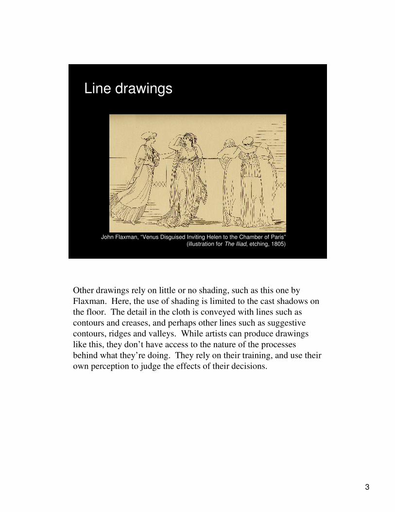
Line drawings

John John FlaxmanFlaxman, “Venus Disguised Inviting Helen to the Chamber of Paris” , “Venus Disguised Inviting Helen to the Chamber of Paris”

(illustration for (illustration for The IliadThe Iliad, etching, 1805), etching, 1805)

Other drawings rely on little or no shading, such as this one by

Flaxman. Here, the use of shading is limited to the cast shadows on

the floor. The detail in the cloth is conveyed with lines such as

contours and creases, and perhaps other lines such as suggestive

contours, ridges and valleys. While artists can produce drawings

like this, they don’t have access to the nature of the processes

behind what they’re doing. They rely on their training, and use their

own perception to judge the effects of their decisions.

4

Ambiguity of lines in images

The ambiguity of projection

• an infinity of 3D curves can project to the same

line in the image

It’s actually a bit surprising that line drawings are effective at all.

Upon first inspection, line drawings seem to be too ambiguous. An

infinity of curves in 3D project to the same line in the image. All

images have this ambiguity, but in photographs there are many other

cues such as shading that help to indicate shape. Here we are

looking just at individual lines.

But it turns out that individual lines contain a wealth of information

about shape. This information is typically local in nature; our

perception is somehow able to integrate all of this into a coherent

whole. Well, sort of.

5

Impossible line drawings

Victor Victor VasarelyVasarely, XICO (silkscreen, 1973), XICO (silkscreen, 1973)

The Penrose triangle (1958)The Penrose triangle (1958)

Line drawings of impossible 3D objects show us that this coherence

is not global. The Penrose triangle, inspired by the work of M.C.

Escher, is perhaps the simplest of the impossible figures. At first, it

appears like an ordinary object. Closer inspection is a bit unsettling,

and its inconsistencies are easily revealed, producing an non-

convergent series of visual inferences (which can be quite fun to

explore). Artists such as Vasarely have pushed this idea even

further, producing vivid imagery that encourages us to explore

several different inconsistent interpretations simultaneously.

6

Interactions between lines

• Interpretation of line drawings depends on

context

after [Barrow 1981]after [Barrow 1981]

Although you might think the Penrose triangle shows that there are

no global effects for visual inference, it’s not that simple. The

figure on the left appears to be raised in the center, while the figure

on the right is flat on the top and bends along its length. Only the

line along the bottom of the drawing differs. Nobody knows

whether we perceive this difference because we integrate local

information consistently, or perform certain types of non-local

inference.

7

Interpretation of line drawings

Labeling of polyhedral scenes

• use an exhaustive catalog of

possible labels of junctions

• determine configurations of

consistent labels using

constraint satisfaction[Waltz 1975]

adapted from [Waltz 1975]adapted from [Waltz 1975]

LL

ForkFork

TT

ArrowArrow

Use of non-local inference is plausible; algorithms exist for

searching among the space of possibilities. Waltz’s method line-

labeling starts with catalogs of all possible line junctions—places

where two or more lines meet. Shown here is the catalog of 18

junctions for classifying trihedral vertices in polyhedral scenes,

where lines are labeled as convex (+), concave (-), or on a boundary

(inside is to the right of the arrow). Then, methods for constraint

satisfaction produce the set of all possible configurations for a

particular picture. For an impossible figure, this set is empty.

8


Labeling for more general scenes

• use larger catalogs of junctions

• rely upon methods to prune unreasonable or

unlikely configurations[Barrow 1981, Malik 1987]

after [after [MalikMalik 1987]1987]

Methods for interpreting line drawings that contain smooth surfaces

extend the junction catalogs and rely upon methods that prune away

large numbers of unreasonable interpretations.

All of these methods label lines with a type; they don’t infer

geometry. Furthermore, they are restricted to lines from contours

and creases, and occasionally lines from shadows.

9


A range of algorithms exist for interpreting

certain types of line drawings

Not very much is known about how humans

process line drawings

However, a lot is known about what

information people could be using for

interpretation

While these algorithms suggest that exhaustive search may be a

viable method for scene interpretation, they don’t say anything

directly about how people interpret line drawings. In fact, not very

much is known about that. Even so, we can still be very specific

about what information is available in a line drawing. This is the

information that our perceptual systems are probably using.

10


Each line in a line drawing constrains the

depicted shape

• The nature of the constraint depends on the

type of line

• The type of the line can sometimes be

inferred from context (within the drawing)

Ambiguity always remains, although some

interpretations are more likely than others

Essentially, each line in a drawing places a constraint on the

depicted shape. In the discussion that follows, we will examine the

information that different types of lines provide. In the end, the

answer is never unique. However, our perceptual systems excel at

discovering the most likely interpretations.

11

Information in line drawings

Lines can mark fixed locations on the shape– creases (sharp folds)

– ridges and valleys

– surface markings (texture features, material boundaries, …)

– hatching lines (although density is lighting-dependent)

Lines can mark view-dependent locations on the shape– contours (external and internal silhouettes)

– suggestive contours

Lines can mark lighting-dependent locations on the shape– isophotes (boundaries of attached shadows or in cartoon shading)

– boundaries of cast shadows

First, we’ll consider lines that mark fixed locations on a shape. This

includes creases, ridges and valleys, and surface markings.

Then, we’ll consider view-dependent lines. The most important is

the contour, which lets us infer surprisingly rich information about

the shape.

There are also lines whose locations are lighting-dependent, such as

edges of shadows; these won’t be discussed here.

Of these, only creases and contours are well understood. Research

on the information other types of lines provide is ongoing.

12

Information in creases

Creases mark discontinuities in surface orientation

– creases are either convex or concave

(this cannot be determined using only local

information)

– there is often a luminance discontinuity in shaded

imagery

concaveconcave

creasecrease

convexconvex

creasecrease

Creases mark orientation discontinuities, and are typically visible in

a real image as a discontinuity in tone.

The crease can be concave or convex; local information doesn’t let

us determine which—algorithms for line labeling only proceeded by

considering all the possibilities, and then enforcing non-local

consistency.

13

Information in ridges and valleys

Ridge and valley lines mark locally rapid changes

in surface orientation

– one possible extension of creases to smooth surfaces

– like creases, they cannot be distinguished using only

local information

Ridges and valleys mark locally maximal changes in surface

orientation. They are often visible in real images as sudden (but

smooth) changes in tone.

The ridges on this rounded cube are particularly effective in

conveying its shape.

14

Information in ridges and valleys

Their use is still unresolved– many ridges and valleys seem to successfully convey shape

– others seem to convey surface markings (inappropriately)

– viewers can locate them in shaded imagery [Phillips 2003]

contourscontours with ridgeswith ridges with valleyswith valleys with bothwith both

Research on the use of ridges and valleys in line drawings is

ongoing. When used alongside contours, ridges and valleys can

often produce an effective rendering of a shape; the valleys on the

side of the horse are successful. In other cases, they look like

markings on the surface of the shape, such as the ridges on its head.

They are reasonable candidates for line drawings, as there is

psychological evidence that viewers can reliable locate ridges and

valleys in shaded imagery.

15

Information in surface markings

Can be located arbitrarily

– but seem to convey shape when they lie along

geodesics (locally shortest paths on the surface)[Stevens 1981, Knill 1992]

– related to perception of texture[Knill 2001]

along geodesicsalong geodesics not along geodesicsnot along geodesics

Markings on a surface can appear as arbitrary lines inside the shape.

However, for a certain type of line known as a geodesic, they can

also convey shape. (Geodesics are lines on the surface that are

locally shortest paths.)

Stevens points out that for many fabricated objects, surface

markings are commonly along geodesics. For a more general class

of surfaces, Knill draws connections between texture patterns and

sets of parallel geodesics.

16

Information in surface markings

Parallel lines in space can also convey shape

– building correspondences between adjacent lines

(using tangents of the curves) lets the viewer infer

the shape[Stevens 1981]

When used in repeating patterns, other curves can be effective as

well. Sets of parallel lines, which are often used to construct plots

of 3D functions, are one notable example. The images that result

are analogous to using a periodic solid texture. Stevens points out

that all one needs to do to infer the shape is to build

correspondences between adjacent lines, matching up points with

equal tangent vectors.

17

Information in hatching

Conveys shape through direction of hatching lines

– more effective when drawn along geodesics[Stevens 1981, Knill 2001]

– lines of curvature are particularly effective[Girshick 2000, Hertzmann 2000]

along lines of curvaturealong lines of curvaturealong geodesicsalong geodesics [Hertzmann 2000]

The use of repeating patterns of lines forms the basis of hatching.

These lines convey shape in two different ways; they convey shape

directly when they are drawing along geodesics. And they convey

shape indirectly through careful control of their density, which can

be used to produce a gradation of tone across the surface.

Particularly effective renderings are obtained when lines of

curvatures are used, which are lines that align with the principal

curvature directions, and also happen to be geodesics. To convey

tone, these lines are used in careful combinations that control their

density in the image.

This concludes the discussion on lines whose locations are fixed on

the shape.

18

Information in contours

For contours, there are two possible situations:

• It comes from a smooth part of the shape– Normal vectors on the surface along the line lie

perpendicular to the viewing direction

• It comes from a crease (or other discontinuity)

Next comes lines whose location on the shape depends on the

viewpoint.

The contours are the most notable example of such lines. There are

two situations when contours are formed. On a smooth surface,

contours are produced when the surface is viewed edge-on. On an

arbitrary surface, contours can also be produced along a crease.

19

Information in contours

The contour generator is the curve sitting on the

surface that projects to the occluding contour

contour generatorcontour generatorcontourcontour

In either case, sitting on the surface is a 3D curve known as the

contour generator. This curve marks all local changes in visibility

across the shape. For a generic (non-singular) viewpoint, the

contour generator consists of a set of isolated loops.

The contour generator projects into the image to become the

contour. Not all parts of the contour are visible.

20

Visibility of contours

Not all parts of the contour generator are visible

• First case: “non-local” occlusions

– Visibility changes occur at T-junctions

– where the viewing direction grazes the surface at

two separated locations (forming a bitangent)

Let’s consider the different cases of visibility for contours.

On a smooth surface, the first case is when one part of the shape

occludes another more distant part. This appears in the image as a

T-junction, where the contour goes behind another part of the shape.

At the location where the visibility changes, the visual ray is tangent

to the surface in two places.

21



• First case: “non-local” occlusions

– The contour continues in back

– and is simply occluded

The contour then continues behind the shape, and is occluded. It is

seen here in this transparent line-drawing of a torus.

22



• Second case: ending contours

– the visible part of the contour ends

– at a cusp in the projection of the contour generator

The second case occurs where the contour comes to an end in the

image. When the occluded part of the contour continues, it does so

at a cusp in the contour.

23




– the tangent of the contour generator lines up with

the viewing direction at this point

This cusp occurs because the contour generator lines up with the

viewing direction, so that its tangent projects to a point.

24




– the radial curvature is zero (the viewing direction

is an asymptotic direction of the surface)

At an ending contour, the radial curvature is zero, which means that

we’re looking along an inflection—an asymptotic direction of the

surface.

25



• Third case: local occlusions (“inside contours”)

– these parts of the contour generator are never

visible; the surface always blocks them

– the radial curvature is negative

The last case is a local occlusion; places where the surface has no

choice but to occlude itself.

These are locations where the radial curvature is negative.

26



• Third case: local occlusions (“inside contours”)

– these contours can be confusing in transparent

renderings

In transparent renderings of contours, one typically does not draw

the local occlusions (which are identified by having negative radial

curvature), as the results can be confusing.

These curves actually correspond to regular contours for an inside-

out version of the surface.

27


The three cases (on smooth surfaces):

visible orvisible or

nonnon--local occlusionlocal occlusion

κκrr > 0> 0

ending contourending contour

κκrr = 0= 0

local occlusionlocal occlusion

κκrr < 0< 0

Here are the three cases, all together.

28

Contours and suggestive contours

Recall: suggestive contours can extend contours

• Extend ending contours at cusps

• Backfacing suggestive contours extend

nonlocally-occluded contours

ContourContour

Suggestive contourSuggestive contour

Inside contourInside contour

NonlocallyNonlocally--occluded contouroccluded contour

Backfacing suggestive contourBackfacing suggestive contour

It’s worth noting that suggestive contours extend true contours at the

ending contour cusps, and that backfacing suggestive contours

always extend nonlocally-occluded (hidden) contours. In other

words, the lines Do The Right Thing.

29

Apparent curvature of contours

The apparent curvature κapp is the curvature of

the contour in the drawing (or image)

• for outward-pointing normal vectors…

• At the cusp of an ending contour, κapp is infinite

κκappapp > 0> 0 κκappapp = 0= 0 κκappapp < 0< 0

Now, let’s consider what the contours look like in the image.

The apparent curvature is simply the curvature of the contour in the

drawing. When working with outward-pointing normal vectors, the

convex parts of the contour have positive apparent curvature, the

concave parts have negative apparent curvature, and it’s zero at the

inflections. At the ending contours, the apparent curvature is

infinite due to the cusp.

30


At a point on the contour (of a smooth surface):

• sign of apparent curvature κapp = sign of Gaussian curvature K

[Koenderink 1984]

• Koenderink proves K = d ⋅ κapp ⋅ κr

– d is the distance to the camera

– κr ≥ 0 for visible points on the contour

convexitiesconvexities correspond tocorrespond to

elliptic regions (elliptic regions (KK > 0)> 0)

concavitiesconcavities correspond tocorrespond to

hyperbolic regions (hyperbolic regions (KK < 0)< 0)

inflectionsinflections correspond to correspond to

parabolic points (Kparabolic points (K = 0)= 0)

Koenderink proved a surprising and important relationship between

the apparent curvature and the Gaussian curvature. Specifically, for

visible parts of the contour on a smooth surface, they have the same

sign. This means we can infer the sign of the Gaussian curvature

simply by looking at the contour.

Koenderink gives a formula that connects these two quantities, that

also involves the distance to the camera (this is because the apparent

curvature gets larger as the object is farther away) and the radial

curvature.

Note that because the radial curvature is never negative for visible

parts of the contour, this allows us to infer the sign of the Gaussian

curvature.

31


• Contours must end in a concave way[Koenderink 1982]

– they only occur where K < 0

• However, the concave ending might be hard to see

K=0K=0

a Gaussian bump viewed from the side towards the topa Gaussian bump viewed from the side towards the top

yesyes nono

A related result is that since ending contours only occur on

hyperbolic regions (where K is negative), the contours must end in a

concave way—approaching their end with negative apparent

curvature.

Even so, in many cases, this concave ending is difficult to discern,

as is the case for a Gaussian bump when viewed from above.

Koenderink and van Doorn also noticed that artists tend to draw

lines that are missing these concave endings.

32

Information in suggestive contours

Relation to contours

• can connect to ending contours

(they line up in the image) [DeCarlo 2003]

– makes it hard to tell where contour ends

Contours are typically easily to detect in real images, at least when

the lighting is right. And there are many studies that demonstrate

how people use them for visual inference.

Suggestive contours are another type of line to draw, and whether

they are in fact detected and represented by our perceptual processes

is still an open question. They do seem to produce convincing

renderings of shape in many cases.

The fact that suggestive contours are an exaggeration of contours to

account for nearby viewpoints is encouraging, as is their property

that they smoothly line up with contours in the image.

33

Information in suggestive contours

Can only appear in hyperbolic regions (K < 0)

• often approach parabolic lines (where K = 0)

away from the contour[DeCarlo 2004]

We can say something about what information they provide. We

know that in many cases that the suggestive contours approach the

parabolic lines away from the contour. They approach it from the

hyperbolic side, as suggestive contours can only appear where K is

negative, as there are no directions with zero curvature where K is

positive. We hope to be able to say more about this in the future.

34

Interior shape features

What lines to draw?

– still not resolved, really

contourscontours contours and contours and

suggestive contourssuggestive contourscontourscontours

and valleysand valleyscontours, ridges contours, ridges

and valleysand valleys

We can compare renderings with ridges and valleys to renderings

with suggestive contours.

On the horse from this viewpoint, the rendering with just valleys is

actually quite convincing. As noted earlier, many of the ridges

appear as surface markings here.

For the valley rendering, some features are missing, but the more

salient features on the side of the horse are depicted. Note that the

slight differences between the lines from suggestive contours, and

from valleys. The shapes they convey do appear to be a little

different. Clearly there is a lot of interesting work to do here.

This concludes our discussion of what information particular lines

provide.

35

Line labeling ambiguity

Different assignments of line labels correspond

to different surfaces

contourcontour

contourcontour

contour orcontour or

suggestivesuggestive

contour??contour??

as a contouras a contouras a suggestive as a suggestive

contourcontour

Of course, this information can only be used if we know the types of

the lines when we’re given a drawing. Earlier we discussed

algorithms for line drawing interpretation; approaches like this are

reasonable to consider for this purpose.

But even if we do use these algorithms, there are often several

different labelings that are consistent. Given the line drawing on the

left which depicts an elliptical shape with a bump, we will

successfully be able to label the green points as contours. The red

point, however, can be either a contour or suggestive contour. Two

possible shapes that match these labelings are shown on the right.

Presumably this problem cannot be solved in general; there will

always be ambiguity. It’s possible that when artists make line

drawings, they are careful to shape the remaining ambiguity so it

won’t be a distraction. These are difficult problems.

36

Projective ambiguity

Even given a line labeling, an infinity of shapes

correspond to that drawing

And even with a line labeling, there is the ambiguity of projection.

At first, this seems hopeless. Yet sketching interfaces like Takeo

Igarashi’s Teddy seem to be quite successful by using “inflation”.

How can this be? Well, there are reasonable constraints on

smoothness that we can expect of the underlying shape. We also

presume that the artist has drawn all of the important lines, so that

no extra wiggles remain.

These issues are the source of one crucial challenge for sketch-based

shape modeling.

37

Bas-relief ambiguity

The projective ambiguity that preserves planarity

– ambiguity in (Lambertian) shaded imagery[Belhumeur 1999]

– preserves contours, shadow boundaries,

(relative) signs of curvature

– has perceptual significance[Koenderink 2001]

We can be even more specific with regard to this ambiguity. It

seems that even for real images, there are well defined ambiguities

for particular types of imagery. One notable example is the

ambiguity that remains when viewing a shape with Lambertian

illumination. It turns out that there is a group of shape distortions

that can be applied to a shape that, with an corresponding

transformation of the lighting positions, produce the same image

(approximately).

The shape distortions here are produced by a three-dimensional

mapping known as the generalized bas-relief transformation. As

shown here, this is the mapping that moves points along visual rays

and also preserves planes. It also preserves contours, boundaries of

shadows, and the relative signs of curvature on the shape.

Perhaps most interestingly is that when you ask people to describe

the shapes they see in shaded imagery, they answer consistently

only up to this ambiguity transformation. How they answer within

this space of possibilities depends on how you ask them.

38

Evaluation of line drawings

How can we tell whether a line drawing is

accurately perceived?

• compare it to drawings by skilled artists

• psychophysical measurement

– resulting shape should be consistent with the shape

used to construct the drawing (modulo ambiguity)

– one study on a hand-made line drawing suggests the

bas-relief ambiguity could be appropriate here [Koenderink 1996]

So how can we be sure that a line drawing we make is perceived

accurately?

Well, one way is to compare that line drawing to one made by a

skilled artist. This is difficult and subjective.

Another way, based in psychophysics, is to simply ask the viewer

questions about the shape they see. If this is done right, you can

reconstruct their percept and compare it to the original shape. When

this comparison is done, it should be with respect to the appropriate

ambiguity transformation.

Koenderink and colleagues have already performed a study like this

on a single line drawing (and compared it to other depictions, such

as shaded imagery). Their results suggest that the bas-relief

ambiguity might be the appropriate ambiguity transformation to use

here.

39

Psychophysical studies

Measurement of perceived shape [Koenderink 2001]

• depth probing

– asks the viewer which point is closer

(green or blue)

So what kinds of questions can you ask viewers?

In psychophysics, the answer is typically – very simple ones, and

lots of them.

Koenderink and colleagues describe a set of psychophysical

methods for obtaining information about what shape a viewer

perceives.

The first they describe is called relative depth probing. The viewer

is shown a display like this one, and simply asked which point

appears to be closer. They are asked this question for many pairs of

points.

40



• depth profile adjustment

– viewer adjusts points until they match the profile of

a particular cross-section

Another method is known as depth profile adjustment. Here, the

viewer adjusts points (vertically) to match the profile of a particular

marked cross-section on the display.

41



• gauge figure adjustment

– viewer adjusts a disk until it appears to sit on the

tangent plane of the surface

Their third method is known as gauge figure adjustment. Here, the

viewer uses a trackball to adjust a small figure that resembles a

thumbtack, so it looks like its sitting on the surface.

All of these methods are successful. But gauge figure adjustment

seems to give the best information given a fixed number of

questions.

part iii: line drawings and...

Documents