BAAABAAA XQQPQQ βαβαµµ

βαβα εδσ == ,2, and&&

From First Principles

PART I – PHYSICAL MATHEMATICS

January 2017 – R4.2Maurice R. TREMBLAY

BAAABAAA XQQPQQ βαβαµµ

βαβα εδσ == ,2, and&&

Chapter 1

To Chrisy

If physical mathematics could explain how I found you, got to know you and Love you still so much today as yesterday… Then the true equation of our life together must be an infinite series of happy moments locked in our memories forever…

MRT

2015

The Greek AlphabetΑ, α, a Alpha άλφαΒ, β, b Beta βήταΓ, γ, g Gamma γάµµα∆, δ, d Delta δέλταΕ, ε, é Epsilon [épsilon] έψιλονΖ, ζ, dz Zeta [dz] ζήταΗ, η, ê Eta [êta] ήταΘ, θ, t Theta [th] θήταΙ, ι, i Iota [eeota] ιώταΚ, κ, k Kappa κάππαΛ, λ, l Lambda λάµδαΜ, µ, m Mu µυ

Ν, ν, n Nu νυΞ, ξ, ks Xi [ks] ξιΟ, ο, o Omicron όµικρονΠ, π, p Pi πιΡ, ρ, r Rho ρώΣ, σ, s Sigma σίγµαΤ, τ, t Tau ταυΥ, υ, u Upsilon ύψιλον

Φ,ϕ,φ, ph Phi φιΧ, χ, kh Chi [kh] χιΨ, ψ, ps Psi ψιΩ, ω, o Omega ωµέγα

These are the equations and phenomenology of the Standard Model of particle physics:

123

110 150120 130 140 GeV100

Super-symmetry Multiverse

MHiggs

?Theory

……Mass

3

2016MRT

This is a Hubble Space Telescope image which features the star cluster Trumpler 14 .

It is one of the largest gatherings of hot massive and bright stars (like our Sun) in the Milky Way, the name of the galaxy our sun is located in.

This cluster houses some of the most luminous stars in our entire galaxy.

2016MRT

4

Mean distance from Earth: 150 million kilometers (149.6 ××××106 km) or 8.31 minutes at the speed of lightAbsolute magnitude: 4.8magMean distance from Milky Way core:~2.5××××1017 km (26,000-28,000 l-y)Galactic period: 2.25-2.50××××108 yVelocity: 217 km/s orbit around the center of the Galaxy, 20 km/s relative to average velocity of other stars in stellar neighborhood. Completes one revolution in about 225–250 million years.Rotation velocity at equator:

7,174 km/hLuminosity: 3.827××××1026 Watts

* 1 Å ==== 1××××10−−−−10 m ==== 0.1 nm (in units wavelength)

The Sun is composed of 73.46 % Hydrogen, 24.85 % Helium and other elements.

2016MRT

Prolog – The Celestial Bodies

The Sun – SOHO 304 Å *

5

The Sun use the principle of nuclear fusion of hydrogen to produce helium and releases the energy that causes stars to shine and hydrogen bombs to explode.

Mean diameter: 1.392××××106

km(109 Earth diameters)

Circumference: 4.373××××106

km(342 Earth diameters)

Oblateness: 9××××10−6

Surface area: 6.09××××1012

km²(11,900 Earth’s)

Volume: 1.41××××1018

km³(1,300,000 Earth’s)

Mass (M ⋅⋅⋅⋅ ): 1.988 435(27)××××1030

kg(~333 Earths)

Surface temperature: 5780K (1K = °°°°C+273)

Core temperature: ~13.6 MK(with M being a Mega or 1M = 1,000,000 = ××××106)

* NEVER LOOK DIRECTLY AT THE SUN:

https://en.wikipedia.org/wiki/Sun† A human eye responds to wavelengths from

about 390 to 700 nm (the 430-770THz frequency)

2016MRT

The Sun – Visible light *†

6

Atmospheric constituents : 78.08% Nitrogen, 20.94% Oxygen, 0.93% Argon, 0.04%(400 parts per million) carbon dioxide, and water vapor trace which varies with climate.

Average orbital speed: 29.783 km/s(107,218 km/h)

Satellites: 1 (the Moon)Mean radius ( ⟨R⊕⟩): 6,372.797 kmMean circumference: 40,041.47 kmSurface area: 510,065,600 km²Land area: 148,939,100 km²

(29.2 %)Water area: 361,126,400 km²

(70.8 %)Volume: 1.083××××10

12km³

Mass (M⊕): 5.9742××××1024

kgEquatorial surface gravity:

9.78 m/s² (1.000 g) Escape velocity: 1,118.6 m/s

(40,269.6 km/h)Equatorial rotation velocity:

465.1 m/s (1,674.4 km/h)2016MRT

The Earth

7

The Moon is in synchronous rotation – it keeps about the same face turned toward Earthat all times. The Apollo missions (11 through 17 with the exception of 13) are shown.

Average orbital speed: 1,022 km/sEquatorial diameter: 3,476.2 km

(0.273 Earth’s) Surface area: 3.793××××10

7km²

(0.074 Earth’s)Volume: 2.1958××××10

10km³

(0.020 Earth’s) Mass: 7.347673××××10

22kg

(0.0123 Earth’s)Volume: 1.083 207 3××××10

12km³

Mass (M): 5.9742××××1024

kgEquatorial surface gravity:

1.622 m/s² (0.1654 g) Escape velocity: 8,568 km/h

(2,000.38 m/s)Equatorial rotation velocity:

4.627 m/s

2016MRT

Apollo 17Apollo 15

Apollo 11(Landing July 20, 1969)

Apollo 16

Apollo 14

Apollo 12

Sea of Tranquility

Alpha

The Moon

8

2016MRT

IntroductionNow that I have pretty much covered all the subject material I set forth to format in Microsoft® Power-Point® (yes I did have a plan and it used rum and progressive elaboration!) I can now revisit the content and tell you why I did this. Believe it or not some people have asked! Back when I was a teenager with modest skills in mathematics (and yet to follow a course on Physics or Chemistry but quite inclined to studying Astronomy) I found a book on Fluid Mechanics in the basement that belonged to my father (a metallurgical engineer who had done work on column flotation). I can still remember bringing it back to my room and my first perusal of it made a significant impact on me because of the appendices – Appendix A showed page after page of long-winded equations while Appendix B showed the key equations of the book (in Cartesian and Cylindrical coordinates). Now that I am writing this, I can say that the first thought I had was: ‘Well, if my Dad can understand this, so can I! ’ Insofar, I graduated from Physics and Engineer-ing Physics and ended up as a Project Manager in a big telecom company’s Network Engineering group!

So, this presentation is meant for some inquisitive 14 year old (I hope he or she finds this in time!); a lib-rary rat like I was that is quite astute at finding things out for himself or herself. To help him along I start with Useful Mathematics as a primer. With that knowledge, even he or she can actually read the rest of the con-tent provided: my compilation of subjects and material that made a contribution in shaping my way of see-ing things (c.f., References). While some like it more abstract and geometrical and others more textual than mathematically inclined, I have had my way in picking, choosing and picturing things and these slides are the result! In this way the Contents highlight some key discussion topics where I have tried as best I could to keep the mathematical technicalities and prerequisites within a logical sequence…

But ever since I have wondered how things would be if I managed to format the key mathematical ideas taken from so many courses and books and made it a necessary prerequisite for a physics novice to dis-cover the beauty and elegance that PART I – PHYSICAL MATHEMATICS brings to one’s understanding of the ‘world’ (or ‘universe’ if I add relativity and gravitation into the mix). The problem over the years (25-35) was that I just kept finding the best stuff in many different books! Eventually, I just started formatting things letting myself flow with the elaborations telling myself that eventually I would fill all the gaps in learning.

9

Now, as for content, we start with the mathematical topic that occupies a prominent place in applied mathematics – infinite series! Students of applied sciences meet infinite series in most of the formulas they use, and it is quite essential that they acquire an intelligent understanding of the concepts under-lying the subject. Vectors are a key subject whether in its mathematical and technical description or its elegant and often uncanny way of picturing things such as position, velocity, or whatever has magni-tude and direction in space. Familiarity with the concepts discussed up to that point is essential to under-standing the rest. I have spent a great deal of time picturing these in 3D so that the reader becomes very comfortable with them in preparation for the higher dimensional (e.g., 4D) version – tensors! Differential equations are also another key technical and crucial mathematical tool for physical mathe-matics to the point that without differential equations there would be no accessible way to formulate a relevant and physical solution that describes a repeatable and predictive behavior that can be verified experimentally. So, formulating and solving differential equations in physics problems is essential to learning physics and a few examples using appropriate and well known techniques (such as would be presented to 1-st year physics or engineering students) are reviewed and applied in exacting detail.

Now, many have asked how I did this. The answer is simple… All my years in a fruitful career have exposedme to Microsoft® Office® products and with time and practice I just came to be adept at format-ting things in either a technical marketing function or an engineering function. The rest was my under-standing of physics with a clear path (with many stops along the way) and a determination to complete this for me alone. So, to you who first browsed your way to this presentation, I hope you will not be discouraged from its inherent length but on the contrary come back to it again and appreciate it too!

2016MRT

10

I do have to stress that the content is in no way original except maybe in its presentation as the Notation to follow outlines. I think this is the originality that is being brought to this material. I have not seen it so well displayed beforehand and frankly, this is my way of learning so I think that this can even plant a seed for learning somehow… Overall, this was a labor of love that took some time to complete (without any financial assistance whatsoever – just a patient wife that was understanding that I had to do this and complete it for posterity). [See Appendix – all of which are available on www.slideshare.net ]

You will notice three primary colors in the slides: Dark Red, Blue and Green. They either are curves, vectors or variables in Figures, variables or terminology within the text, bold italic terms (e.g., how something is called – either mathematical or physical) or even to help in focusing on ‘results’ such as equations boxed with one of these colors: • Dark Red is good for skimming through and paying attention to the ‘key stuff’; • Blue is the ‘from first principles’ part (and pretty much the reason for doing this so

anything blue you need to read through to understand the whole thing!) and; • Green is the ‘physical part’ where the subject matter (i.e., the physics) is highlighted. Otherwise, these colors just makes for a nicer presentation! Italics are also used to spell out key terms (e.g.,of variables and/or constants),Bold italics are important definitions .

Since mathematics is a language you will be able to peruse a slide by homing onto the mathematics which is set in black. Scalars are typically black italic (e.g., the Cartesian coordinates x, y or z) while vectors are typically black bold (e.g., the position vector r ). This applies to constants, variables, &c. This presentation is key in developing a sense of ‘reading’ the physics through ‘reading’ equations… It was the reason why I did this –to be able to peruse the slides and take on the whole whopping content in order to assimilate a result, equation, complex term or mathematical or physical conclusion.

Notation“Now you may ask, ‘ What is mathematics doing in a physics lecture? ’ We have several possible excuses: first, of course, mathematics is an important tool, but that would only excuse us for giving the formu la in two minutes. On the other hand, in theoretical phys ics we discover that all our laws can be written in mathematical form; and that this has a certain simp licity and beauty about it. So, ultimately, in orde r to understand nature it may be necessary to have a dee per understanding of mathematical relationships.”Richard Feynman, Feynman Lectures on Physics, Vol. I, Chap. 22, § 22- 1 (1964).

2016MRT

11

Contents of 5-Chapter PART I

PART I – PHYSICAL MATHEMATICSUseful Mathematics and Infinite SeriesDeterminants, Minors and CofactorsScalars, Vectors, Rules and ProductsDirection Cosines and Unit VectorsNon-uniform AccelerationKinematics of a Basketball ShotNewton’s LawsMoment of a VectorGravitational AttractionFinite RotationsTrajectory of a Projectile with Air

ResistanceThe Simple PendulumThe Linear Harmonic Oscillator The Damped Harmonic OscillatorGeneral Path RulesVector CalculusFluid MechanicsGeneralized Coordinates

2016MRT

The Line IntegralVector TheoremsCalculus of VariationsGravitational PotentialKinematics of ParticlesMotion Under a Central ForceParticle Dynamics and OrbitsSpace Vehicle DynamicsComplex FunctionsDerivative of a Complex Function Contour IntegralsCauchy’s Integral FormulaCalculus of ResiduesFourier Series and Fourier TransformsTransforms of Derivatives Matrix OperationsRotation TransformationsSpace Vehicle MotionAppendix

“The enormous usefulness of mathematics in the natur al sciences is something bordering on the mysterious and that there is no rational explanatio n for it.” Eugene Wigner, ‘The unreasonable effectiveness of mathematics in the natural science s.’ Richard Courant lecture in mathematical sciences delivered at New York University, May 11, 1959 (196 0).

12

Contents

PART I – PHYSICAL MATHEMATICSUseful Mathematics and Infinite SeriesDeterminants, Minors and CofactorsScalars, Vectors, Rules and ProductsDirection Cosines and Unit VectorsNon-uniform AccelerationKinematics of a Basketball ShotNewton’s LawsMoment of a VectorGravitational AttractionFinite RotationsTrajectory of a Projectile with Air

ResistanceThe Simple PendulumThe Linear Harmonic Oscillator The Damped Harmonic OscillatorGeneral Path RulesVector CalculusFluid MechanicsGeneralized Coordinates

2016MRT

The Line IntegralVector TheoremsCalculus of VariationsGravitational PotentialKinematics of ParticlesMotion Under a Central ForceParticle Dynamics and OrbitsSpace Vehicle DynamicsComplex FunctionsDerivative of a Complex Function Contour IntegralsCauchy’s Integral FormulaCalculus of ResiduesFourier Series and Fourier TransformsTransforms of Derivatives Matrix OperationsRotation TransformationsSpace Vehicle MotionAppendix

13

The natural numbers are the positive integers such as one, two, three:

Useful Mathematics

Irrational numbers (i.e., the quotient or fraction of one integer with another) have decimal digits:

2016MRT

The complex numbers are real numbers with one new number i whose square is −1:

12 −=i

...7

22

2

3

8

5

2

1,,,,

is rational but:

LL 82.71828182e 141592654.3π == :number Euler :Pi &is irrational (note the ellipsisL ). The real numbers include the rational numbers and the irrational numbers; they correspond to all the points on an infinite line called the real line.

...1428.37

225.1

2

3625.0

8

55.0

2

1,,,, ====

and zero, 0. Negative numbers are labeled by −1,−2,−3,&c. (et cetera - ‘and so forth’ ). The Prime numbers are 2,3,5,7,11,13,17,… and are natural numbers greater than 1 that have no positive divisors other than 1 and itself. Rational numbers are ratios of integers:

14

Addition is a mathematical operation that represents the operation of adding objects to a collection (or to the total amount of objects together in a collection). It is signified by the plus sign (+) and is expressed with an ‘equals’ sign (=) as in 2+3=5 (N.B., this is the same commutative result as 3+2=5 – N.B., nota bene - ‘note well’ ). When it is written mathematically it looks like:

The plus sign can also serve as a unary operator that leaves its operand unchanged (i.e., +x means the same as x – i.e., id est - ‘that is’ ). This notation may be used when it is desired to emphasise the ‘positiveness’ of a number, especially when contrasting with the negative (+5 vs −5 – vs , versus - ‘against’).

and so on:

11245633422111 =++=+=+=+ and,,

123333 =+++

A negative number is a real number that is less than zero (i.e., <0). Such numbers are often used to represent the amount of a loss or absence. Negative numbers are usually written with a minus sign (−) in front (e.g., −3 represents a negative quantity with a magnitude of three, and is pronounced ‘minus three’ or ‘negative three’ – e.g.,exempli gratia - ‘for example’ or ‘for instance’).

Subtraction is a mathematical operation that represents the operation of removing objects from a collection. It is signified by the minus sign (−). 2016

MRT

15

2016MRT

The division operation 20÷4=5(inverse of 4×5=20).

Division is another arithmetic operation denoted by (÷). Specifically, if b times c equals a. Written mathematically:

where b is not zero, then a divided by b equals c, which means, when written arithmetic mathematically:

cba ×=

Multiplication (often denoted by the cross symbol (×) or by the absence of symbol). The multiplication of two whole numbers is equivalent to the addition of one of them with itself as many times as the value of the other one (e.g., 3 multiplied by 4 – often said as ‘3 times 4’) can be calculated by adding 3 copies of the quantity/number 4 together. Written mathematically, we have:

Here 3 and 4 are the factors and 12 is the product – the result of multiplication – not addition (c.f., 3+3+3+3=12– c.f. , confer - ‘compare’ ).

12333343933422111 =+++=×=×=×=× and,,

cba =÷

5420 =÷For instance (see Figure):

since 4×5=20.

In the expression a÷b=c, a is called the dividend or numerator, b the divisor or denominator and the result c is called the quotient.

16

Exercise: Memorize the Base 10 Multiplication Table shown. What are the common factors and what do they represent - physically? What do the diagonal elements mean?

17

Algebra is a generalized arithmetic in which symbols are used in place of numbers. Al-gebra thus provides a language in which general relationships can be expressed among quantities (e.g., a, b, x, y, &c.) whose numeral values need not be known in advance. The arithmetical operation of addition, subtraction, multiplication, and division have the same meanings in algebra. The symbols of algebra are normally letters of the alphabet.

cba =+If we subtract b from a to give the difference d, we would write:

dba =−Multiplying a and b together to give e may be written in any of these ways:

ebaebaebaeba ===⋅=× ))((Whenever two algebraic quantities are written together with nothing between them (i.e., like ab=e above), it is understood that they are to be multiplied.

Dividing aby b to give the quotient (a fraction) f is usually written (‘≡ ’ means ‘equivalent’):

fb

aba =≡÷

If we have two quantities a and b and add them to give a sum c, we could write:

but it may sometimes (especially in exponentials) be more convenient to write:

fba =2016MRT

18

In order of priority, parentheses (i.e., (…)) are used first and brackets (i.e., […] ) are used second to show the order in which various operations are to be performed. Thus:

fed

cba =−+ )(

means that, in order to find f , we are first to add a and b together, then multiply their sum by c and divide by d, and finally subtract e. If () and [] are used, choose curly brackets .

27123 =+x

An equation is simply a statement that a certain quantity is equal to another. Thus 7+2=9, which contains only numbers, is an arithmetic equation, while:

which contains a symbol as well (i.e., the unknown variable x), is an algebraic equation. The symbols in an algebraic equation usually cannot have any arbitrary (i.e., unspeci-fied) values if the equality is to hold. Finding the possible values of these symbols is called solving the equation. The solution of the latter equation above is:

5=x2016MRT

since only when x is 5 is it true that 3x+12=27(i.e., 3⋅5+12=15+12=27 QED. N.B., Latin QED – quod erat demonstrandum – meaning ‘which had to be demonstrated’).

19

In order to solve an equation , a basic principle must be kept in mind: Any operation performed on one side of an equal sign must also be performed on the other side.

153

122712123

=

−=−+

x

x

To check a solution, we substitute it back in the original equation and see whether the equality is still true. Thus we can check that x=5 by reducing the original algebraic equation to an arithmetical one (where the symbol ‘⇒ ’ means ‘implies’):3x+12=27⇒(3)(5)+12=27⇒15+12=27⇒27=27.

An equation therefore remains valid when the same quantity, numerical or otherwise, is added to or subtracted from both sides, or when the same quantity is used to multiply or divided both sides of the equal sign (=). Other operations, for instance squaring ( ²) or taking the square root (√ ), also do not alter the equality if the same thing is done to both sides. As a simple example, to solve 3x+12=27above, we subtract 12 from both sides:

To complete the solution we divide both sides by 3:

53

15

3

3

=

=

x

x

2016MRT

20

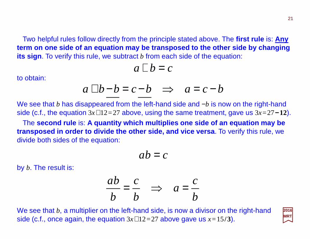
Two helpful rules follow directly from the principle stated above. The first rule is: Anyterm on one side of an equation may be transposed t o the other side by changing its sign . To verify this rule, we subtract b from each side of the equation:

cba =+

by b. The result is:

to obtain:

cba =

2016MRT

bcabcbba −=⇒−=−+We see that b has disappeared from the left-hand side and −b is now on the right-hand side (c.f., the equation 3x+12=27above, using the same treatment, gave us 3x=27−−−−12).

The second rule is: A quantity which multiplies one side of an equation may be transposed in order to divide the other side, and v ice versa . To verify this rule, we divide both sides of the equation:

b

ca

b

c

b

ba =⇒=

We see that b, a multiplier on the left-hand side, is now a divisor on the right-hand side (c.f., once again, the equation 3x+12=27above gave us x=15/3).

21

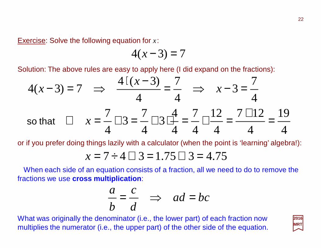
Exercise: Solve the following equation for x:

7)3(4 =−xSolution: The above rules are easy to apply here (I did expand on the fractions):

2016MRT

4

19

4

127

4

12

4

7

4

43

4

73

4

74

73

4

7

4

)3(47)3(4

=+=+=⋅+=+=∴

=−⇒=−⋅⇒=−

x

xx

x

that so

When each side of an equation consists of a fraction, all we need to do to remove the fractions we use cross multiplication :

bcadd

c

b

a =⇒=

What was originally the denominator (i.e., the lower part) of each fraction now multiplies the numerator (i.e., the upper part) of the other side of the equation.

22

or if you prefer doing things lazily with a calculator (when the point is ‘learning’ algebra!):

75.4375.1347 =⊕=⊕÷=x

Exercise: Solve the following equation for y:

2016MRT

2

3

2

5

−=

+ yySolution: First we cross multiply to get rid of the fractions, and then solve in the usual way:

82

16

2

2

162

10635

63105

)2(3)2(5

=

=

=+=−

+=−+=−

y

y

y

yy

yy

yy

23

y=8 is the final answer. If you solved this on your own, give yourself a million bucks!

Two rules for multiplying and dividing positive and negative quantities are straightforward. The first rule is: Perform the indicated operation on the absolute value of the quantity (e.g., the absolute value of −7 is 7). The second rule is: If the quantities are both positive or both negative, the result is positive :

Here are a few examples:

2016MRT

b

a

b

a

b

aabbaba +=

−−==−−= and))(())((

If one quantity is positive and the other negative the result is negative :

215

3070)7)(10(3

2

6

20)5)(4(45

2018)3)(6(

−=−−=−−=−

−=−=−−=−−

and,

,,,

b

a

b

a

b

aabbaba −=

−=−−=−=− and))(())((

24

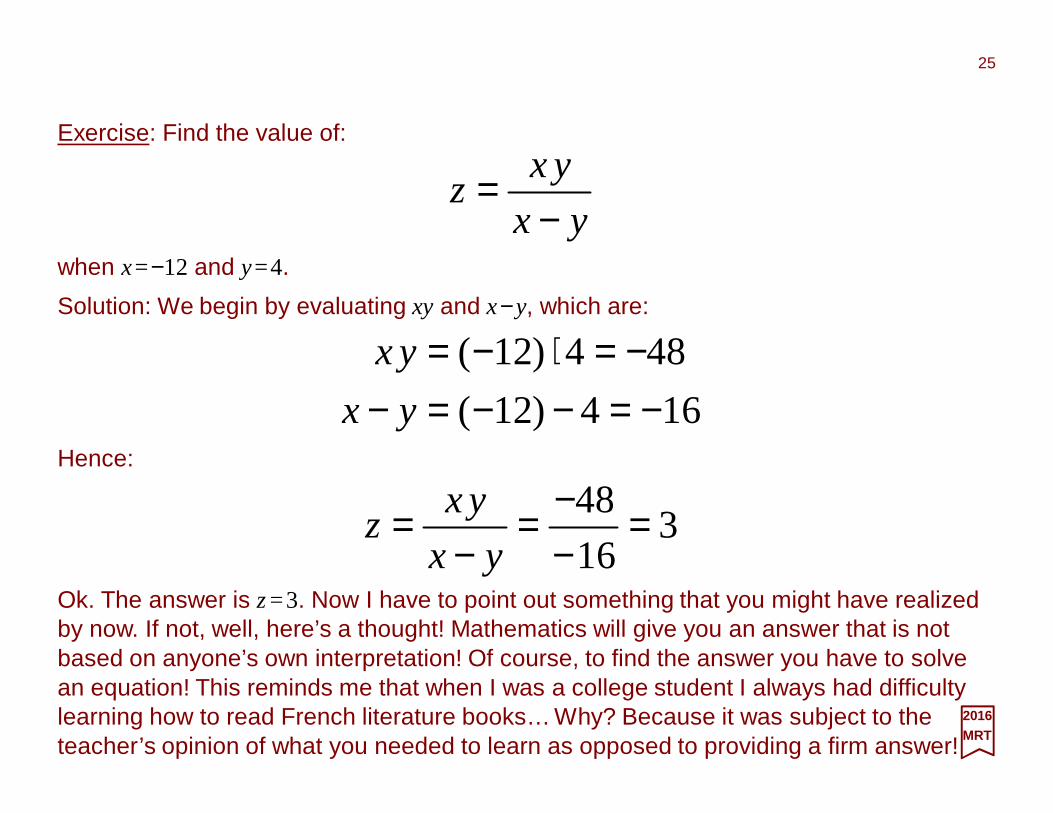
Exercise: Find the value of:

2016MRT

yx

yxz

−=

Solution: We begin by evaluating xy and x−y, which are:

164)12(

484)12(

−=−−=−−=⋅−=

yx

yx

when x=−12 and y=4.

Hence:

316

48 =−−=

−=

yx

yxz

25

Ok. The answer is z=3. Now I have to point out something that you might have realized by now. If not, well, here’s a thought! Mathematics will give you an answer that is not based on anyone’s own interpretation! Of course, to find the answer you have to solve an equation! This reminds me that when I was a college student I always had difficulty learning how to read French literature books… Why? Because it was subject to the teacher’s opinion of what you needed to learn as opposed to providing a firm answer!

It is often necessary to multiply a quantity by itself a number of times. This process is indicated by a superscript number called the exponent, according to the following scheme:

When we multiply a quantity raised to some particular power (say An) by the same quantity raised to another power (say Am), the result is that quantity raised to a power equal to the sum of the original exponents. That is:

2016MRT

4321 AAAAAAAAAAAAAA =⋅⋅⋅=⋅⋅=⋅= and,,We read A2 as ‘A squared’ because it is the area of a square of length A on a side; similarly A3 as ‘A cubed’ because it is the volume of a cube of whose sides is A long. More generally we speak of An as ‘A to the n-th power’ – A4 is ‘A to the 4-th power’, &c.

)( mnmn AAA +=For example:

75252 AAAA == +

which we can verify directly by writing out the terms:

7)()( AAAAAAAAAAAAAAA =⋅⋅⋅⋅⋅⋅=⋅⋅⋅⋅⋅⋅

26

From the above result we see that when a quantity raised to a particular power (say An) is to be multiplied by itself a total of m times, we have:

since:

2016MRT

mnmn AA =)(For example:

63232)( AAA == ⋅

6)222(22232)( AAAAAA ==⋅⋅= ++

27

Reciprocal quantities are expressed in a similar way with the addition of a minus sign in the exponent, as follows:

It is important to remember that any quantity raised to the zeroth power, e.g., A0, is equal to 1. Hence:

2016MRT

44

33

22

1 1111 −−−− ==== AA

AA

AA

AA

and,,

Exactly the same rules as before are used in combining quantities raised to negative powers with one another and with some quantities raised to a positive power. Thus

6)71(7123443

2)2(1213)25(25

)(

)(−−−−⋅−−

−⋅−−−−−

===

====

AAAAAAA

AAAAAAA

and

,,

10)22(22 === −− AAAAThis is more easily seen if we write A−2 as 1/A2:

11

2

2

2222 ==⋅=−

A

A

AAAA

28

The square root has that name because the length of each side of a square of area Ais given by √A. Some examples of square roots are as follows:

2016MRT

22 93339

25.425.6565.625.42

100101010100

164441611111

AAAAA =⋅=

=⋅=

=⋅=

=⋅==⋅=

.

because

andbecause

,because

,because,because

The square root of a number less than 1 is larger than the number itself:

49.07.07.07.049.0

01.01.01.01.001.0

=⋅=

=⋅=

because

andbecause

29

The square root of a quantity may be either positive or negative because (+A)(+A)=(−A)(−A)=A2. Using the exponents we see that, because:

2016MRT

we can express square roots by the exponent ½:

AAAA === ⋅ 1)21(2221 )(

21AA =Other roots may be expressed similarly. The cube root of a quantity A, written ,

when multiplied by itself twice equals A. That is:

3 A

AAAAA ==⋅⋅ 33333 )(which may be more conveniently written:

1)31(3331 )( AAA == ⋅

where . 313 AA =

30

In general the n-th roots of a quantity, , may be written A1/n, which is a more convenient form for most purposes. Some examples may be helpful:

2016MRT

161)41)(41(4141

1)3)(31(313

47)41)(7(741

41)21)(21(2121

2)21)(4(4214

2)4)(21(2144

)(

)(

)(

)(

)()(

)(

AAA

AAA

AAA

AAAA

AAAA

AAAA

==

==

==

===

===

===

−−−

−−−

and

,

,

,

,

n A

31

An equation that involves power or roots or both is subject to the same basic principles that govern the manipulation of simpler equations: Whatever is done to one side must be done to the other. Hence the following rules: An equation remains valid when both sides are raised to the same power, that is, when e ach side is multiplied by itself the same number of times as the other side and An equation remains valid when the same root is taken on both sides an equal sign .

2016MRT

Exercise: Newton’s (1642-1727) law of gravitation states that the force F between two massive bodies whose masses are m1 and m2 a distance r apart is given by the formula:

where G is a universal constant. Solve this formula for r and explain its proportionality. Solution: We begin by transposing r 2 with F to give:

and finally we take the square root √ of both sides:

The distance r is proportional to the square root of the product of the masses, √(m1⋅m2), and inversely proportional to the square root of the force between them, 1/√F . The constant of proportionality would be the square root of the universal constant,√G≡G½.

221

r

mmGF =

F

mmGr 212 =

Fmmr

F

mm

F

mmG

F

mmG

F

mmGrr

121

212121212 ⋅⋅∝⇒⋅

∝⋅=⋅=⋅==

32

Quadratic equations , which have the general form:

2016MRT

02 =++ cxbxaare often encountered in algebraic calculations. The term quadratic describes something that pertains to squares, to the operation of squaring, &c. Many physical phenomena involve quadratic behavior such as dropping a ball from the roof of a building and calcu-lating the distance s travelled as a function of time gives: s=½gt2. The time t is quadratic!

a

cabbx

a

cabbx

2

4

2

4 22 −−=

−−= −+

−−−−++++and

By looking at these formulas, we see that the nature of the solution depends upon the value of the quantity b2−4ac. When b2=4ac, √(b2−4ac)=0 and the two solutions are equal to just x=−b/2a. When b2>4ac, √(b2−4ac) is a real number and the solutions x+and x− are different. When b2<4ac, √(b2−4ac) is the square root of a negative number, and the solutions are different. The square root of a negative number is called an imagi-nary number because squaring a real number, whether positive or negative, always gives a positive number: (+2)2=(−2)2=+4, hence √(−4) cannot be either +2 or −2.

In such an equation, a, b, and c are constants. A quadratic equation is satisfied by the values of x given by the formulas:

33

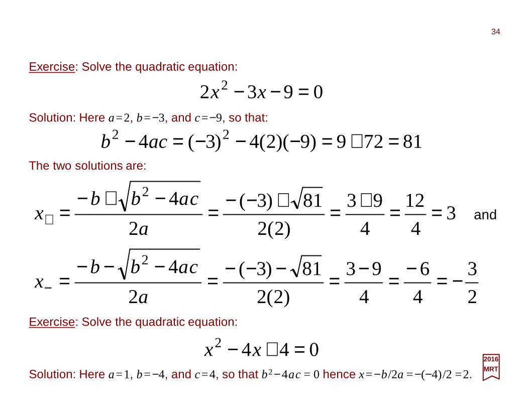
Exercise: Solve the quadratic equation:

2016MRT

0932 2 =−− xxSolution: Here a=2, b=−3, and c=−9, so that:

The two solutions are:

81729)9)(2(4)3(4 22 =+=−−−=− acb

2

3

4

6

4

93

)2(2

81)3(

2

4

34

12

4

93

)2(2

81)3(

2

4

2

2

−=−=−=−−−=−−−

=

==+=+−−=−+−

=

−

+

a

cabbx

a

cabbx and

Exercise: Solve the quadratic equation:

0442 =+− xxSolution: Here a=1, b=−4, and c=4, so that b2−4ac= 0 hence x=−b/2a =−(−4)/2 =2.

34

A right triangle is a triangle, two sides of which are perpendicular. Such triangles are frequently encountered in physics, and it is necessary to know how their sides and angles are related. The hypotenuse of a right triangle is the side opposite the right angle, as shown in the Figure. It is always the longest side. The three basic trigonometric functions, the sine, cosine, and tangent of an angle, are defined as follows:

ehypothenus

side adjacentand

ehypothenus

side opposite ====c

b

c

a θθ cossin

2016MRT

A right triangle – 2 sides of which are perpendicular.

θb = Adjacent side

a=

Opp

osite

sid

e

ϕ

o90

tancossin

222 =+=+

===

ϕθ

θθθ

cba

b

a

c

b

c

a

90°

side adjacent

side opposite====b

a

cb

ca

θθθ

cos

sintan

From these definitions we see that:

Numerical values of sinθ , cosθ , and tanθ for angles from 0°to 90°. These figures may be used for angles from 90° to 360° with the help of the Table:

f (θ ) θ 90° + θ 180° + θ 270° + θ

sinθ sinθ cosθ −sinθ −cosθcosθ cosθ −sinθ −cosθ sinθtanθ tanθ −1/tanθ tanθ −1/tanθ

For example, if we require the value of sin120°, we first note that 120° = 90° + 30°. Then, since sin(90° + θ )= cosθ we have sin120° = sin(90° + 30°) = cos30° = 0.866.

35

2

1

1

The inverse of a trigonometric function is the angle whose function is given. For instance, the inverse of sinθ is the angle θ . If sinθ =x, then the angle θ may be designated as θ =arcsinx or as θ =sin−1x. It is important to keep in mind that an expression such as sin−1x does not mean 1/sin−1x. The inverse trigonometric functions are:

xxx

x

is whoseangle sine=≡=

=−1sinarcsin

sin

θ

θ

2016MRT

zzz

z

is whoseangle tangent=≡=

=−1tanarctan

tan

θθ

yyy

y

is whoseangle cosine=≡=

=−1cosarccos

cos

θθ

and:

and, finally, the ratio of the above two:

Inverse functions are cotanθ =1/tanθ , secθ =1/sinθ (i.e., secant) and cosecθ =1/cosθ .

36

To solve a given triangle means to find the values of any unknown sides or angles in terms of the values of the known sides and angles. A triangle has three sides and three angles, and we must know the values of at least three of these six quantities, including one of the sides, to solve the triangle for the others. In a right triangle, one of the angles is always 90°, and so all we need here are the lengths of any two of its sides or the lengths of one side and the value of one of the other angles to find the remaining sides and angles.

θθθθ

sinsintantan

ac

c

aba

b

a =⇒==⇒= and

2016MRT

Suppose we know the length of the side b and the angle θ in the right triangle of the previous Figure. From the definitions of sine and tangent we see that:

This gives us the two unknown sides a and c. To find the unknown angle ϕ, we can use any of these formulas:

=

=

= −−−

a

b

c

a

c

b 111 tancossin ϕϕϕ or,

Alternatively, we can use the fact that the sum of the angles in any triangle is 180°. Because one of the angles in a right triangle is 90°, the sum of the other two must be 90°! Hence, since θ +ϕ =90° we get ϕ =90°−θ here.

37

Another useful relationship in the right triangle is the Pythagorean theorem, which states that: The sum of the squares of the sides of such a trian gle adjacent to the right angle is equal to the square of its hypotenus e. For the triangle in the previous Figure:

2016MRT

Thus we can always express the length of any of the sides of the right triangle in terms of the other sides:

Exercise: In the triangle in the previous Figure, a=7cm and b=10cm. Find c, θ , and ϕ .

222 cba =+

222222 bacacbbca +=−=−= or,

Solution: From the Pythagorean theorem:

cmcmcmcm 2.1214910049107 2222 ==+=+=+= bacSince tanθ =a/b:

o35)7.0(tan10

7tantan 111 ==

=

= −−−

cm

cm

b

aθ

The value of the other angle ϕ is given by ϕ =90°−θ =90°−35° =55°.

38

f (x)

xO

Secant

Tangent

yo

xo

Po

P

∆x= dx

dy∆x

θ

Now we complicate things… We define the derivative of a function y= f (x) at the point x which is defined as the slope of the tangent to a function at the point x (see Figure).

The difference quotient is the slope of the secant through the points P(x,y) and Po(xo,yo):

o

o)()()(

xx

xfxf

x

xf

x

y

−−

=∆

∆=∆∆

2016MRT

Derivative of a function f (x).

The differential quotient f ′(x) is the limit (i.e., identified by the mathematical terminology lim) value of the difference quotient for P→Po and ∆x→0:

x

xfxxf

x

yxf

xd

ydxx ∆

−∆+=∆∆=′≡

→∆→∆

)()(limlim)(

00

The derivative of a function at the point Po corresponds to the gradient of its graph at the point Po, f ′(xo)= tanθ (i.e., the magnitude of the rate of increase of the graph is the slope).

39

Applying ‘derivation’ comes with a set of rules . An effort of memorization is needed…

2016MRT

Factor rule : A constant factor c remains unchanged when the derivative is taken:

0=xd

cd

xd

xfdc

xd

xfcd )()]([ ⋅=⋅

Constant rule : The derivative of a constant c is equal to zero:

Power rule : When carrying out the derivative of a power function, the exponent is lowered by unity, and the old exponent enters as a factor:

1−⋅= nn

xnxd

xd

Sum rule : The derivative of a sum (or difference) is equal to the sum (or difference) of the derivatives:

xd

xgd

xd

xfd

xd

xgxfd )()()]()([ ±=±

40

Product rule (N.B., These can be written shorthand by letting u≡ f (x), v≡g(x), &c.):

2016MRT

Quotient rule :

)()()(

)()(

)()(

)()()]()()([

)()(

)()(

)()]()([

xhxgxd

xfdxh

xd

xgdxf

xd

xhdxgxf

xd

xhxgxfd

udvvduvudxd

xfdxg

xd

xgdxf

xd

xgxfd

⋅⋅+⋅⋅+⋅⋅=⋅⋅

+=⇔⋅+⋅=⋅

Chain rule :

xd

xgd

xgxd

xgd

xgxd

d

xg

xd

xgdxf

xd

xfdxg

xd

xgxfd

xg

xf

xd

d

)(

)(

1)]([

)(

1

)(

)()(

)()(

)]()([

)(

)(

2

1

2

1

−==

⋅−⋅=⋅=

−

−

gd

fd

xd

gd

xd

fd

xgd

xgfd

xd

xgd

xd

xgfd ⋅=⋅= or)(

)]([)()]([

where d f/dg is called the exterior derivative and d g/dx is the interior derivative.

41

Logarithmic derivative : The derivative of the logarithm lny of the function y for y>0:

2016MRT

xd

yd

yy

xdyd

xd

yd 1ln ==

42

Exercise: Find the derivative of y= f (x)=expx/(1+x)≡ex/(1+x) (not y=exp[x/(1+x)] ≡ex/(1+x)). Solution: Let g(x)=expx and h(x)=1+x (i.e., where the function f (x) is the quotient of functions g(x) and h(x): f (x)=g(x)/h(x).

1)(

)(e)(

)( ==′==′xd

xhdxh

xd

xgdxg x ,

We use the quotient rule, f ′(x)=df (x)/dx=[h(x)g′(x) − g(x)h′(x)]/h2(x), to find the derivative of the function f (x):

since g′(x)=expx and h′(x)=1 and h2(x)=(1+x)2. Simplifying the algebra will then give us:

22 )1(

)1(ee)1(

)1(

)()e()()1()(

x

x

x

xhxgxxf

xxx

+−+=

+′−′+=′

2)1(

e)(

x

xxf

x

+=′

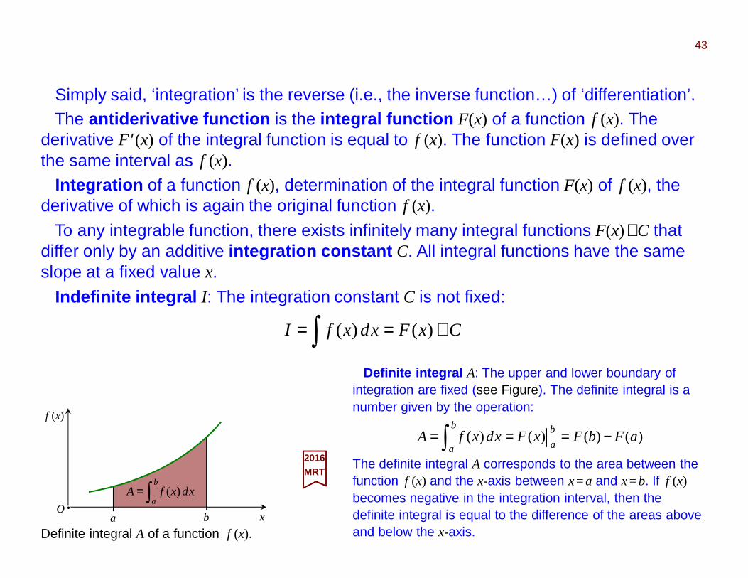
Simply said, ‘integration’ is the reverse (i.e., the inverse function…) of ‘differentiation’. The antiderivative function is the integral function F(x) of a function f (x). The

derivative F ′(x) of the integral function is equal to f (x). The function F(x) is defined over the same interval as f (x).

Integration of a function f (x), determination of the integral function F(x) of f (x), the derivative of which is again the original function f (x).

To any integrable function, there exists infinitely many integral functions F(x)+C that differ only by an additive integration constant C. All integral functions have the same slope at a fixed value x.

Indefinite integral I: The integration constant C is not fixed:

f (x)

xO

a b

2016MRT

Definite integral A of a function f (x).

Definite integral A: The upper and lower boundary of integration are fixed (see Figure). The definite integral is a number given by the operation:

The definite integral A corresponds to the area between the function f (x) and the x-axis between x=a and x=b. If f (x)becomes negative in the integration interval, then the definite integral is equal to the difference of the areas above and below the x-axis.

)()()()( aFbFxFxdxfAb

a

b

a−=== ∫

CxFxdxfI +== ∫ )()(

43

∫=b

axdxfA )(

Applying ‘integration’ also comes with a set of rules .

2016MRT

( )11

1

−≠+

=+

∫ nn

xxdx

nn

Constant rule : A constant factor C may be pulled out of the integral

Sum rule : The integral over the sum (or difference) of terms is equal to the sum (or difference) of the integrals over the terms:

Power rule :

Inversion rule : Inversion of the sign of the definite integral under inversion of the integration boundaries:

∫∫∫ ±=± xdxgxdxfxdxgxf )()()]()([

∫∫ −=a

b

b

axdxfxdxf )()(

∫∫ ⋅=⋅ xdxfCxdxfC )()(

44

By n≠−1we mean that n cannot take a value that equals −1 since it would then become a singular (as in ‘singularity’) integral which would lead to an term being divided by zero.

Equality of upper and lower boundary : The integral vanishes if the interval is a=a:

2016MRT

Interval rule : Definite integrals may be decomposed into integrals over parts of the interval ab that can be split in two intervals ac and cb:

Partial integration : Also called integration by parts which is the inversion of the product rule of differentiation:

Substitution rule :

0)( =∫a

axdxf

∫∫∫ +=b

c

c

a

b

axdxfxdxfxdxf )()()(

∫∫ ⋅−⋅=⋅ xdxgxd

xfdxgxfxd

xd

xgdxf )(

)()()(

)()(

( ))()()(

)]([ xgzzdzfxdxd

xgdxgf ==⋅ ∫∫

Logarithmic integration :

Cxfxdxd

xfd

xf+=⋅∫ )(ln

)(

)(

1

45

F (x)f (x) f ′(x)F (x)f (x)

Now we show the derivatives and integrals of elementary functions as given below in the Table where the original function f (x), its derivative f ′(x)=df (x)/dx and the integral function ∫ f (x)dx=F (x)+C are displayed respectively.

2016MRT

c 0 xc

221 x1x

11

1 ++

aa

x1−axaax

x1 21 x− xln

xsin xcos xcos−

xcos xsin− xsin

xtan x2cos1 xcosln−

xsinlnx2sin1−xcot

xe xe xe

aax lnaax lnxa

xxx −lnx1xln

xalog ax ln1 axxx ln)ln( −

xarcsin 211 x− 21arcsin xxx −+xarccos 211 x−− 21arccos xxx −−

xarctan 211 x+ )1(lnarctan 221 xxx +−

)1(lncotarc 221 xxx ++211 x+−xcotarc

46

f ′(x)

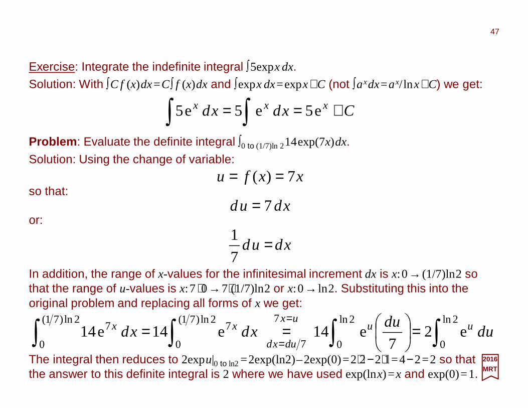
Exercise: Integrate the indefinite integral ∫5expx dx.

2016MRT

47

Solution: With ∫C f (x)dx=C∫ f (x)dx and ∫expx dx=expx+C (not ∫axdx=ax/ lnx+C) we get:

Cxdxd xxx +== ∫∫ e5e5e5

Problem : Evaluate the definite integral ∫0 to (1/7)ln 214exp(7x)dx.

Solution: Using the change of variable:

xxfu 7)( ==so that:

xdud 7=or:

xdud =7

1

In addition, the range of x-values for the infinitesimal increment dx is x:0→ (1/7)ln2so that the range of u-values is x:7⋅0→7⋅(1/7)ln2or x:0→ ln2. Substituting this into the original problem and replacing all forms of x we get:

∫ ∫∫∫ =

===

=

2ln

0

2ln

0

7

7

2ln)71(

0

72ln)71(

0

7 e27

e14e14e14 udud

xdxd uuux

duxd

xx

The integral then reduces to 2expu|0 to ln2 =2exp(ln2)–2exp(0)=2⋅2−2⋅1=4−2=2 so that the answer to this definite integral is 2 where we have used exp(lnx)=x and exp(0)=1.

We will now summarize the essentials of infinite series without detailed proofs.

48

=⇔= ∑

=∞→∞→

k

nn

kk

kwsss

1

limlim

2016MRT

Infinite sequences and series are important in mathematical physics. Let w1,w2,…,wn,…be a sequence of numbers (real or complex). If we define an infinite series as being:

(N.B., limk – from1to ∞ – is called the limit as k approached infinity) then the series Σn=1tokwn (N.B., Σn – from 1 to k – is called the summation sign over n) is said to be convergent . The number s is called the sum (or value) of the series and is given by:

)11( 2 −=⇒−=+= iibiaswhere:

∑∑∞

=

∞

=

==11 n

nn

n vbua and

for wn=un+ ivn, a complex number with both un and vn real (N.B., ibid for s=a+ ib above).

Now, if the series:

...3211

+++=∑∞

=

wwwwn

n

is convergent, thenΣn=1to∞ wn is said to beabsolute convergent . If Σn=1to∞wn is conver-gent but Σn=1to∞ |wn| diverges, then Σn=1to∞wn is said to be conditionally convergent .

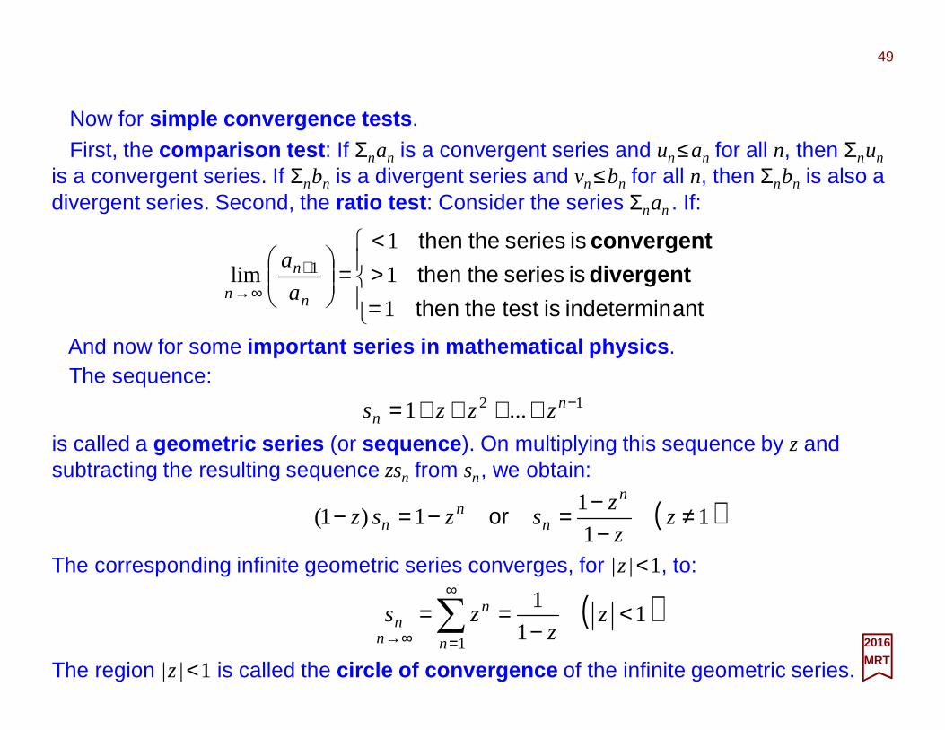
Now for simple convergence tests .

49

=><

=

+∞→

antindetermin is test the then

is series the then

is series the then

1

1

1

lim 1 divergent

convergent

n

n

n a

a

2016MRT

And now for some important series in mathematical physics . The sequence:

12 ...1 −++++= nn zzzs

is called a geometric series (or sequence ). On multiplying this sequence by z and subtracting the resulting sequence zsn from sn, we obtain:

( )11

11)1( ≠

−−=−=− z

z

zszsz

n

nn

n or

The corresponding infinite geometric series converges, for |z|<1, to:

( )11

1

1

<−

==∑∞

=∞→z

zzs

n

n

nn

The region |z|<1 is called the circle of convergence of the infinite geometric series.

First, the comparison test : If Σnan is a convergent series and un≤an for all n, then Σnun

is a convergent series. If Σnbn is a divergent series and vn≤bn for all n, then Σnbn is also a divergent series. Second, the ratio test : Consider the series Σnan. If:

Now for a series of functions : Consider:

50

)(...)()()( 21 zuzuzuzs nn +++=

2016MRT

and:

( )Nnzszfzuzszf nn

nnn

≥<−== ∑∞

=∞→

all forif ε)()()()(lim)(1

where N is independent of z in the region a≤|z|≤b and ε is an arbitrarily small quantity greater than zero, then the series sn(z) is said to be uniformly convergent in the closed region a≤|z|≤b.

∑∫∫ ∑∫∞

=

∞

=

==11

)()()(n

b

an

b

an

n

b

azdzuzdzuzdzf

The derivative of f (z):

∑∑∞

=

∞

=

=11

)()()(

nn

nn zu

zd

dzu

zd

d

zd

zfdequals

only if un(z), and dun(z)/dzare continuous in the region and Σndun(z)/dz is uniformly convergent in the region.

If the individual terms, un(z), of a uniformly convergent series are continuous, the series may be integrated term by term, and the resultant series will always be convergent. Thus:

A determinant is a square array of quantities called elements an,bn,cn,…, rn (n≠0) which may be combined according to the rules given below. In symbolic matrix form, we write:

51

nnnn rcba

rcba

rcba

L

MOMMM

L

L

2222

1111

=∆

2016MRT

Here n is called the order of the determinant. The value of the determinant (i.e., the outcome of calculating ∆ ) in terms of the elements ai,bj,ck,…, rl is defined as:

∑=∆n

jikjikji rcba

l

ll L,...,,

...ε

where the Levi-Civita symbol, ε i j k…l, has the following property:

−+

=repeated isindex an if

of npermutatio odd an for

of npermutatio even an for

0

),,,,(1

),,,,(1

... lK

lK

l kji

kji

kjiε

=−=+

=)(0

)132,213,321 (1

)312,231,123 (1

Otherwize

if

if

kji

kji

kjiε

For example:

Determinants, Minors and Cofactors

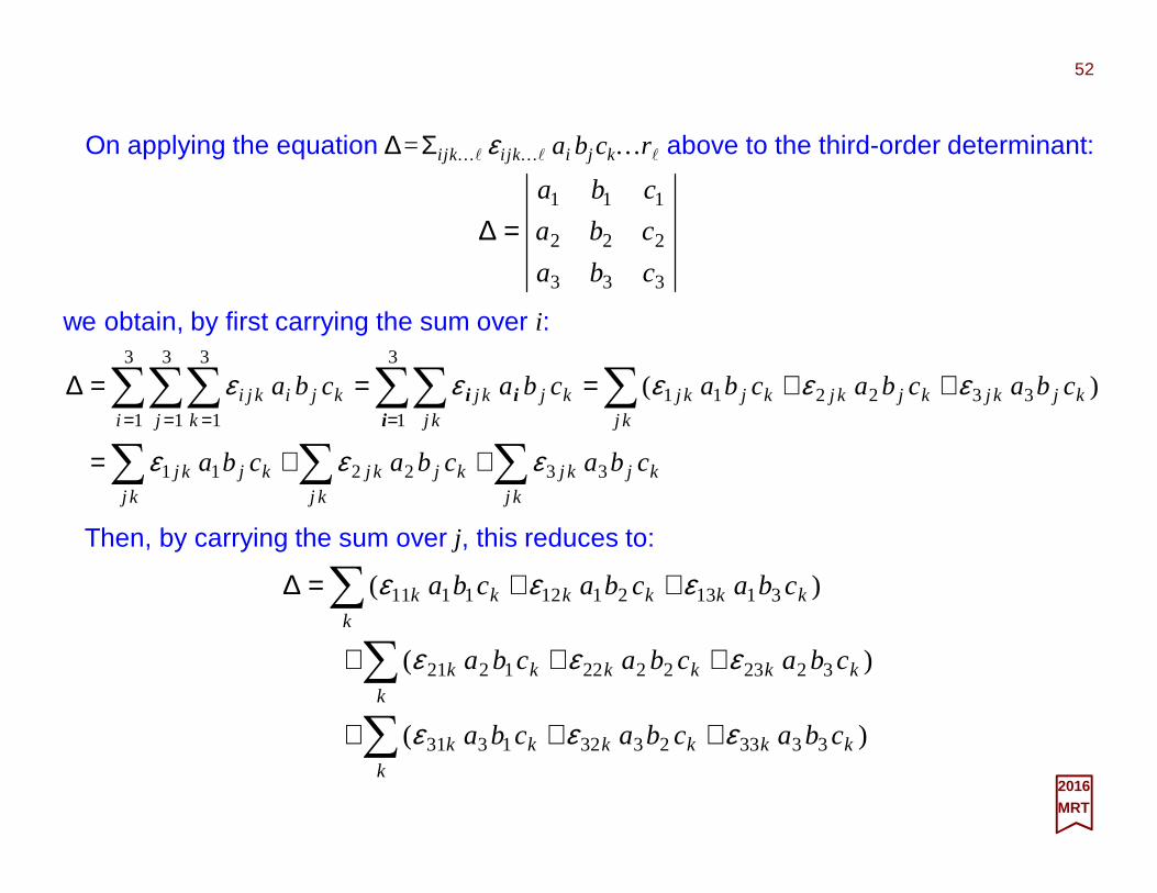
On applying the equation ∆=Σijk…l ε i jk…l ai bj ck…rl above to the third-order determinant:

52

333

222

111

cba

cba

cba

=∆

2016MRT

we obtain, by first carrying the sum over i:

Then, by carrying the sum over j, this reduces to:

∑∑∑

∑∑∑∑∑∑

++=

++===∆== = =

kjkjkj

kjkjkj

kjkjkj

kjkjkjkjkjkjkj

kjkjkj

i j kkjikji

cbacbacba

cbacbacbacbacba

332211

332211

3

1

3

1

3

1

3

1

)(

εεε

εεεεεi

ii

∑

∑

∑

+++

+++

++=∆

kkkkkkk

kkkkkkk

kkkkkkk

cbacbacba

cbacbacba

cbacbacba

)(

)(

)(

333323321331

322322221221

311321121111

εεε

εεε

εεε

333

222

111

)( 312231123

213132321

123213132

312231321

cba

cba

cba

cbacbacba

cbacbacba

cbacbacba

cbacbacba

++−+++=∆

−++−−=∆

or

−−−−

++++

++++

++++

−−−−−−−−

which finally reduces to (i.e.,a formulafora third-order determinant):

Since ε11k=ε22k=ε33k=0 (i.e., an index is repeated) the equation above becomes:

53

2016MRT

and finally expanding the rest, by finally carrying the sum over k, we get:

000 233213313223122131132112 ++++++++=∆ ∑∑∑∑∑∑k

kkk

kkk

kkk

kkk

kkk

kk cbacbacbacbacbacba εεεεεε

323332223232123132

313331213231113131

332323232223132123

312321212221112121

331133231132131131

321312221212121112

cbacbacba

cbacbacba

cbacbacba

cbacbacba

cbacbacba

cbacbacba

εεεεεεεεεεεεεεεεεε

+++

+++

+++

++++++

++=∆

With the aid of the property for ε i jk, the above equation means that:

323223123313213113332232132

312212112331231131321221121

)0()0()1()0()1()0()0()0()1(

)1()0()0()0()1()0()1()0()0(

cbacbacbacbacbacbacbacbacba

cbacbacbacbacbacbacbacbacba

++−+++++++++−++++−+++++=∆

a3b2c1

a1b2c3 a3b1c2a2b3c1

a1b3c2 a2b1c3

+a2b3c1

+a1b2c3

+a3b1c2 −a3b2c1

−a1b3c1

−a1b3c1

The result of the previous equation can be written in the form:

54

22

113

33

112

33

221

122131331223321 )()()(

cb

cba

cb

cba

cb

cba

cbcbacbcbacbcba

+−=

−+−−−=∆

2016MRT

where:

233233

22 cbcbcb

cb−=

is called the minor of this determinant. The procedure of expressing ∆ in the form above may be generalized to obtain the

value of the n-th-order determinant. In the last few sides we saw that the expansion of a third-order determinant is expressed as a linear combination of the product of an element and a second-order determinant. Careful examination of the above equations reveals that the second-order determinant is the determinant obtained by omitting the elements in the row and column in which the multiplying element appears in the original determinant. The resulting second-order determinant is called a minor . Thus the minor of a1 is obtained in the following way:

33

221

333

222

111

cb

cba

cba

cba

cba

:therefore isof minor The

out

In the general n-th-order determinant, the sign (−1)i + j is associated with the minor of the element in the i-th row and the j-th column. The minor with its sign (−1)i + j is called the cofactor . For the determinant:

55

nnnn

n

n

aaa

aaa

aaa

AA

L

MOMM

L

L

11

12221

11211

det ==

2016MRT

the value in terms of cofactors is given by the Laplace (1749-1827) development :

( )iAaAAn

j

jiji det

1

any for∑=

==

Expanding this along the first row gives i =1. For example:

1212

1111

2

1

11

2221

1211 AaAaAaAaa

aaA

j

jj +==⇔= ∑

=

where:

2121212112

2222221111 )1()1( aaaAaaaA −=−=−==+=−= ++ and

On substituting this last result into the expression for |A|, we obtain the number:

21122211 aaaaA −=

The following are properties of determinants (i.e., their inherent rules):

56

321

321

321

333

222

111

ccc

bbb

aaa

cba

cba

cba

==∆

2016MRT

1. The value of a determinant is not changed if corresponding rows and columns are interchanged (N.B., this is more appropriately called transposing along the diagonal), e.g.:

2. If a multiple of one column is added (row by row) to another column or if a multiple of one row is added (column by column) to another row, the value of the determinant is unchanged,e.g.:

3333

2222

1111

333

222

111

cbbka

cbbka

cbbka

cba

cba

cba

+++

=

3. If each element of a column or row is zero, the value of the determinant is zero,e.g.:

0000

333

111

=cba

cba

4. If two columns or rows are identical, the value of the determinant is zero,e.g.:

57

2016MRT

0

111

222

111

=cba

cba

cba

5. If two columns or rows are proportional, the value of the determinant is zero,e.g.:

0

2

2

2

133

222

111

=caa

caa

caa

6. If two columns or rows are interchanged, the sign of the determinant is changed,e.g.:

333

222

111

333

222

111

abc

abc

abc

cba

cba

cba

−=

7. If each element of a column or row is multiplied by the same number, the resulting determinant is multiplied by that same number,e.g.:

333

222

111

333

222

111

abc

abc

abc

k

ckba

ckba

ckba

=

As the story goes, on the evening of October 16, 1843, William R. Hamilton (1805-1865) was walking with his wife along the Royal Canal in Dublin when the answer leap-ed to his mind, the fruit of years of reflection. With his penknife he then and there carved on a stone on Broom Bridge the fundamental formula for quaternion multiplication:

58

zyx iiiiii σσσσσσσσσσσσ −=−=−=−=−=−=−=−=−= 321213132ˆˆˆ kji and,

kji ˆ10

01ˆ0

0ˆ01

10321 ii

i

ii zyx ==

−===

−===

= σσσσσσ and,

1ˆˆˆˆˆˆ 222 −==== kjikji

312212222222222

322

21 1ˆˆˆˆˆˆ σσσσσσσσ iiii =−==−−−=++=++ andkjikji

=≠

=

−+−

=)(1

)(0

321

213

ji

ji

i

iji

kkk

kkkk δ

δδδδδδ

σ

This also means that they all take on the form (Exercise):

which in today’s notation is provided using the Pauli matrices σ in the directions 1,2,or3:

The Pauli matrices, σ k, can be written using:

which means that:

or x, y, and z as shown, and where the imaginary number is i =√(−1), or otherwise:

2016MRT

10110

01det1)(0

0

0det110

01

10det 3

221 −=−−=

−=−==−−=

−=−=−== σσσ and, iii

i

i

bc

a

θ

In a plane (e.g., a sheet of 8½×11 paper on a large table)

dVector dcomes out from the front of the sheet!

rrrr

O

where the symbol ×××× (cross product) represents the vector product . In the Figure, the variable θ is the angle between the vectors a and c. Notice how this new vector d provides a way to reach out, mathematically, into another dimension!

Vectors , on the other hand, are ‘oriented’ objects and the vector ‘addition’ rule is:

Examples of vectors are: position R, displacement d, velocity v, acceleration a, force Fand torque ττττ, all of which are characterized buy the fact that they also provide direction !

a c====++++ b

c××××ad ====

Adding the vectors a and b together produce a

resultant vector c. The product of the vectors aand c, respectively, produces a new vector d.

rrrr

rrrr

rrrr

rrrr rrrrrrrr

Scalars are quantities represented by magnitude only. For example: mass m, volume V, density ρ (i.e., m/V ), energy E and temperature T. The magnitude is represented by the ‘absolute value’ symbol |…| which means | a |= | ±a | =a, the magnitude of the vector a.

rrrr rrrr

One of the key properties of vectors is the capability of generating a new vector from the product of two vectors on a plane – this new vector will be perpendicular (out of page):

ˆ

×××× ====

ˆ

kj

i

ˆˆ

ˆ

kj

i

ˆˆ

ˆ

kj

i

ˆˆ

i j k ×××× ====j k i ×××× ====k i jand

×××× ====i i 0 ×××× ====j j 0 ×××× ====k k 0

2016MRT

rrrr rrrr

With this definition, we can create an orthogonal basis for a vectors space in three dimensions consisting in mutually perpendicular unit vectors i, j and k:

Scalars, Vectors, Rules and Products

ˆ ˆ

T

m

E

59

rrrrrrrr

rrrrrrrr rrrr rrrr

rrrr

ac

θb

In Space (e.g.,look around!)

d Vector d comes out from bottom of the sheet

rrrr

O

e

Unit vector ecomes out from the top of the plane

ˆ

ˆ

c×××× = a sinθad = c

The vector product is given by:

The scalar product is given by:

The vector commutativity addition rule is given by (i.e., the ‘sum’ order is irrelevant!):

c ==== a ++++ b a++++b====

c××××ad ==== c ×××× a==== −

Adding arbitrarily the vectors a and b together

produce a resultant vector c. The product of

the vectors a and c, respectively, produces a

vector d and the angle θ is shown.

rrrr

rrrrrrrr

rrrr

rrrr

rrrr

while the vector associativity addition rule – introducing a new vector e (e.g., a unit ‘normal to the plane’ vector) – is:

e( b++++a b++++a====)++++ e ++++ ( )

where the scalar product symbol ‘ • ’ (dot product) of a

vector a with a vector b. rrrr rrrr

The magnitude of the vector product of two vectors can be constructed by taking the product of the magnitudes of the vectors times the sine of the angle (<180 degrees) between them.

b• = ba cosθ b a•=a

where the symbol ‘ ×××× ’ (cross product) represents the vector product whereas the magnitude of this new vector is:

ˆ

2016MRT

ˆˆ

60

The position vector , R, of an object located at a PointP(R) =P(X,Y,Z) is then given in a ‘Cartesian’ coordinate system as a function of Cartesian unit vectors : I , J and K :

The angles αααα, ββββ, and γγγγ are the angles that OPmakes with the three coordinate axes. Here we have X= Rl, Y= Rm, and Z= Rnwhere l = cosαααα, m=cosββββ, and n= cosγγγγ (with 1=l2 + m2 + n2). The quantities l, m, and n are called direction cosines .

Now the fun stuff begins… In the language of line segments (i.e., OA, AB, BP, OP, &c –see Figure), an object located at P from an origin O is represented by the relation:

BPABOA ++≡The position of a physical object is completely specified by its position vector (some-times called radius vector). To start with, the position vector is a vector drawn (pretty much) from the origin of a (say Cartesian) coordinate system to the object in question.

ˆ

The vectors RX I , RYJ and RZ K are three components of R ; they are the vector representations of the projections of Ron the three coordinate axes, respectively. The quantities RX, RY, and RZ are the magnitudes of the vector components in the three respective directions (e.g., in Cartesian: X, Y, and Z). Using the Pythagorean theorem:

ˆ

1

ˆcosˆcosˆcos

=

++=≡

and

KJI

2016MRT

!

)()()()(222

22222

ZYX

BPABOA

++=

++==

R

R

RRR ZYX

=++=

++==

)ˆcosˆcosˆ(cos

ˆˆˆ

KJI

KJI

Direction Cosines and Unit Vectors

ˆ ˆ

ˆ ˆ

61

ˆ

KJ I

ˆˆ

Y

X

Z

Rαααα

ββββ

γγγγ

P(x,y,z)BA

ROC

RR

R

R

ROP

OP

αααα ββββ γγγγ

OP R

R

αααα ββββ γγγγ

r•••• P

r

ϕr • r

r

ϕ ab

a××××b14243

| r |cosϕ

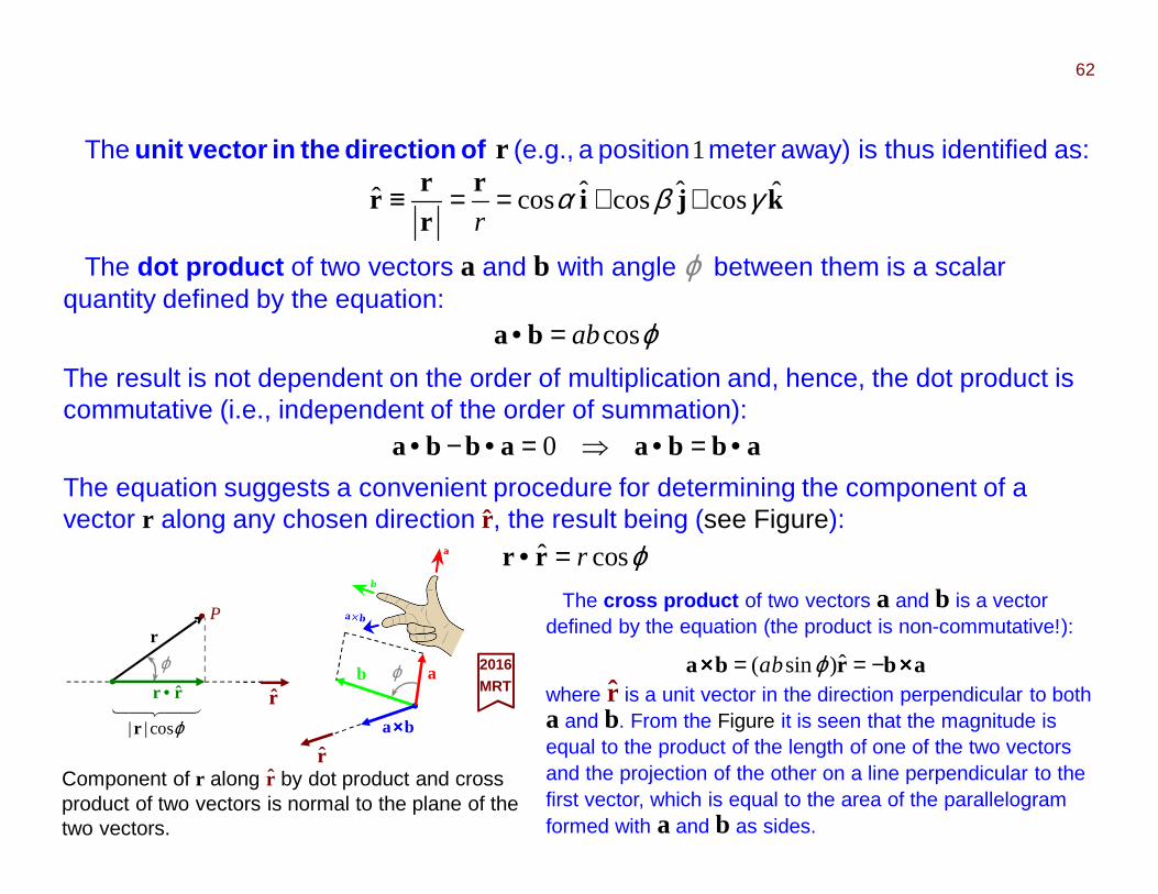
The unit vector in the direction of r (e.g., a position1meter away) is thus identified as:

The dot product of two vectors a and b with angle ϕ between them is a scalar quantity defined by the equation:

The cross product of two vectors a and b is a vector defined by the equation (the product is non-commutative!):

where r is a unit vector in the direction perpendicular to both a and b. From the Figure it is seen that the magnitude is equal to the product of the length of one of the two vectors and the projection of the other on a line perpendicular to the first vector, which is equal to the area of the parallelogram formed with a and b as sides.

The result is not dependent on the order of multiplication and, hence, the dot product is commutative (i.e., independent of the order of summation):

kjir

rr

r ˆcosˆcosˆcosˆ γβα ++==≡r

ϕcosab=•ba

abbaabba •=•⇒=•−• 0

The equation suggests a convenient procedure for determining the component of a vector r along any chosen direction r , the result being (see Figure):

ϕcosˆ r=• rr

abrba ×××××××× −== ˆ)sin( ϕbaˆ

Component of r along r by dot product and cross product of two vectors is normal to the plane of the two vectors.

2016MRT

ˆ

ˆ

62

When resolved into rectangular (i.e., Cartesian) components, the dot product is:

2016MRT

ijk

kjkiji

0kjkikj0jikiji0

kkjkikkjjjijkijiii

kkjkikkjjjijkijiii

kjikjiba

ˆ)(ˆ)(ˆ)(

)ˆˆ)(()ˆˆ)(()ˆˆ)((

)ˆˆ()ˆˆ()ˆˆ()ˆˆ()ˆˆ()ˆˆ(

)ˆˆ()ˆˆ()ˆˆ()ˆˆ()ˆˆ()ˆˆ()ˆˆ()ˆˆ()ˆˆ(

ˆˆˆˆˆˆˆˆˆˆˆˆˆˆˆˆˆˆ

)ˆˆˆ()ˆˆˆ(

yzzyzxxzxyyx

yzzyxzzxxyyx

yzxzzyxyzxyx

zzyzxzzyyyxyzxyxxx

zzyzxzzyyyxyzxyxxx

zyxzyx

babababababa

babababababa

babababababa

bababababababababa

bababababababababa

bbbaaa

−−−=

−−−=

+=

=

=

=

++++++++

××××++++××××++++××××

××××++++××××−−−−××××++++++++××××−−−−××××++++××××++++

××××++++××××++++××××++++××××++++××××++++××××++++××××++++××××++++××××

××××++++××××++++××××++++××××++++××××++++××××++++××××++++××××++++××××

++++++++××××++++++++××××

↑↑↑↑

since i ×××× j =k (j ×××× i =−k), j ××××k = i (k ×××× j =−i) & k ×××× i = j (i ××××k =−j ) and i ×××× i =0, j ×××× j =0 & k ××××k =0. The result of the cross product can be conveniently expressed by the determinant:

ˆ ˆ ˆ ˆ ˆ ˆ ˆ ˆ ˆ ˆ ˆ ˆ ˆ ˆ ˆ ˆ ˆ ˆ ˆ ˆ ˆ ˆ ˆ ˆ

zzyyxx

zzyzxzzyyyxyzxyxxx

zzyzxzzyyyxyzxyxxx

zyxzyx

bababa

bababababababababa

bababababababababa

bbbaaa

++=

•••••••••=

•••••••••=

•=•

)ˆˆ()ˆˆ()ˆˆ()ˆˆ()ˆˆ()ˆˆ()ˆˆ()ˆˆ()ˆˆ(

ˆˆˆˆˆˆˆˆˆˆˆˆˆˆˆˆˆˆ

)ˆˆˆ()ˆˆˆ(

kkjkikkjjjijkijiii

kkjkikkjjjijkijiii

kjikjiba

++++++++++++++++++++++++++++++++

++++++++++++++++++++++++++++++++

++++++++++++++++

since i •••• j = j •••• i =0, j ••••k =k •••• j =0 & k •••• i = i ••••k =0 and i •••• i =1, j •••• j =1 & k ••••k =1 while the cross product becomes:

ˆ ˆ ˆ ˆ ˆ ˆ ˆ ˆ ˆ ˆ ˆ ˆ ˆ ˆ ˆ ˆ ˆ ˆ

kjikji

kji

ba ˆ)(ˆ)(ˆ)(ˆˆˆ

ˆˆˆ

xyyxxzzxyzzyyx

yx

zx

zx

zy

zy

zyx

zyx bababababababb

aa

bb

aa

bb

aa

bbb

aaa −−−=+== ++++−−−−−−−−××××↑↑↑↑↑↑↑↑

63

Certain multiple products of vectors are occasionally encountered and we list two of the most common ones in the following:

cbabcacbabacacbcba )()()()()()( ••=•=•=• −−−−×××××××××××××××××××× and

Exercise: Find a++++b and a−−−−b for a=2i −−−− j ++++k and b= i −−−−3j −−−−5k. ˆ ˆ ˆ ˆ ˆ ˆ

Exercise: What is the direction cosines of the vector 2i −−−−2j −−−−4k. ˆ ˆ ˆ

Exercise: Find the unit vector perpendicular to i −−−−2j −−−−3k and i ++++2j −−−−k. ˆ ˆ ˆ ˆ ˆ ˆ

Exercise: Find a•b××××c if a=2i , b=3j , and c=4k . ˆ ˆ ˆ

Exercise: Show that a=2i −−−− j ++++k, b= i −−−−3j– 5k, and c=3i −−−−4j −−−−4k form the sides of a right triangle [HINT: What equation do you need to show that two vectors are perpendicular?]

ˆ ˆ ˆ ˆ ˆ ˆ

Exercise: If ai −−−−2j ++++k is perpendicular to i −−−−2j −−−−3k, find a. ˆ ˆ ˆ ˆ ˆ ˆ

Exercise: a) Calculate the distance from P1(−1, −4,5) to P2(3,−2,2). b) What are the direction cosines of P1P2? c) What is the equation of the line connecting P1 and P2?

Exercise: Show that a=i++++4j ++++3k and b=4i ++++2j −−−−4k are perpendicular. ˆ ˆ ˆ ˆ ˆ ˆ

Exercise: Find the angle between 2i and 3i ++++4k. ˆ ˆ ˆ

Exercise: Find the component of 8i ++++ j in the direction of i ++++2j −−−−2k. ˆ ˆ ˆ ˆ ˆ

Exercise: Compute (a××××b) ××××c and a×××× (b××××c) directly for a=2i ++++2j , b=3i– j ++++k, and c=8i . ˆ ˆ ˆ ˆ ˆ ˆ

ˆ ˆ ˆ

Exercise: Show that (p−−−−eA) ×××× (p−−−−eA)= iehB where p= –ih∇∇∇∇, B=∇∇∇∇ ××××A, i =√(−1), e and h are constants while ∇∇∇∇= i ∂/∂x++++ j ∂/∂y++++k ∂/∂z. Physically, A is just a vector potential. ˆ ˆ ˆ

I definitely suggest that you attempt these exercises as to appreciate these concepts:

2016MRT

64

Spe

ed, v

[mi/h

]

Useful unit conversions:• 1 mile [mi]=1.61kilometers [km]• 1 foot [ft]=0.3048meter [m].• 1 km=1000m=103 m. • 1 m=3.281ft. • 1 mi=5280ft. For this example, we have: • 5 mi/h=8 km/h=2.2m/s.*• 10 mi/h=16.09 km/h=4.2m/s. • 50 mi/h=80.47km/h=37.8m/s. • 100mi/h=160.93km/h=71.5m/s.

. 2.2 3600

1

1

10

1

1.6

1

5.0 0.5

3

sm

sh

kmm

mikm

hmi

hmi =

=

2016MRT

a) Determine the average acceleration in mi/h/s for each of the three speeds; b) Suppose that the acceleration is constant (i.e., uniform Acceleration) from rest until

the shifting from 3rd to 4th speed. What would be the distance traveled?c) Determine the real distance traveled up to the shifting from the 3rd to the 4th speeds.

* For example, to convert ‘mi/h’ into ‘m/s’:

For this non-uniform acceleration stuff, there is pretty much no better way than to look over an example such as an accelerating 1966 Alpha Romeo GT and calculating it!

1st-2nd

2nd-3rd

3rd-4th

Time, t [s]The graph below represents the speed, v, as a function of time, t, of a 1966 Alpha Romeo GT. (Reprinted from Road and Track, November 1986.)

Non-uniform Acceleration65

Time, t [s]

Spe

ed, v

[mi/h

]

2016MRT

1st-2nd

2nd-3rd

3rd-4th

a) Using a=∆v/∆t= (vf −vi)/(tf − ti) (see Plot below), we get • up to 1st → 2nd: 9.2 mi/h/s (~15 km/h/s);• up to 2nd → 3rd: 4.8 mi/h/s (~8 km/h/s); • up to 3rd → 4th: 3.2 mi/h/s (~5 km/h/s).b) Using P1: (0s,0mi/h) and P2: (17s,84 mi/h), we get a=4.94 (mi/h)/s (~8 km/h/s). Then, by checking units and using the kinematics formula and solving for s= (vf

2−vo2)/2a, we

get the distance 2000 ft . c) 1200 ft .

(4s,37mi/h)

(9.5s,61mi/h)

(17s,84mi/h)

smi/hssmi/hmi/h

/2.904

03721 =

−−=→a

smi/hss

mi/hmi/h/8.4

5.45.9

371632 =

−−=→a

smi/hssmi/hmi/h

/2.31071

614843 =

−−=→a

)( 2tfv =

∆v

t [s]

v [mi/h]

9.5 s4.5 s

37 mi/h

61 mi/h

if

if

tt

vv

t

va

−−

=∆∆=

The slope of a v(t) plot:∆t

This acceleration is considered to be constant from rest until the shifting from 3rd to 4th speed: a = (vf –vo)/(tf – to)

= (84 – 0)/(17 – 0) a≅ 5mi/h/s

P1

P2

is the acceleration a(t).

66

α

θo

Efficiency in service delivery:

otan2tan θα −=Lh

vo

L

2016MRT

† Basketball players in the United States of America would understand g as: The speed of an object in free-fall will increase by 32 feet per second with each second it falls or 32 ft/s2, which is always directed towards the center of the Earth.

* The time (t-) dependent parabolic trajectory of a basketball isgiven by (g/2)t 2 + (vo)t + (so − s) = 0 which is of the parametricform k1t2+ k2t + k3 = 0 where k1=|g|/2, k2= |vo| and k3= |so−−−− s| areparameters of the trajectory. Note that the absolute valuemeans |x | = |±x| = x.

Kinematics of a Basketball ShotA player throws a basketball with an initial velocity vo=|vo| along an initial angle θo

towards a hoop situated at a horizontal distance L and at a height h above the throw stance. Assume no air-resistance,nor jump from the player,nor rotationof the basketball. Show that the scalar initial velocity required to reach the hoop is given by the relation:

)(tancos2 oo2o Lh

Lgv

−=

θθThe symbol g represents the constant acceleration

due to Earth’s gravity (∼10 meters per second, per second or 10 m/s2 †) and is given by (we will see why later):

where G is Newton’s constant of universal attraction (6.673×10−11 m3/kg/s2), M⊕ is the mass of the Earth (5.9742×1024 kg) and R⊕ is the equatorial radius of the Earth (6,378,100m).

2⊕

⊕=R

MGg

67

A basketball follows a path in xy-t Space-Time –showing a parabolic trajectory.*

2010

PMOAllstream

z

F

y

F

x

F zyx

∂∂+

∂∂

+∂

∂=• F∇∇∇∇

Point P at the tip of the distance vector r is given in Rectangular (Cartesian) Coordinates by the intersection of constant x, constant y and constant zplanes (i.e., a box in 3D!) – relative to the frame of the basketball.

zyx ˆˆˆz

f

y

f

x

ff

∂∂

∂∂

∂∂= ++++++++∇∇∇∇

zy

x

zyx

F

ˆˆ

ˆ///

ˆˆˆ

∂∂

−∂

∂

∂∂

−∂

∂

∂∂

−∂∂

=∂∂∂∂∂∂=

y

F

x

F

x

F

z

F

z

F

y

F

FFF

zyx

xyzx

yz

zyx

++++++++

++++××××∇∇∇∇

2

2

2

2

2

2

z

f

y

f

x

fff

∂∂+

∂∂+

∂∂=•=∇2 ∇∇∇∇∇∇∇∇

y

x

r

P

ˆ

kj

i

ˆ

ˆ

k

i

ˆ

Constant y plane

j

Constant x plane

kjirr ˆˆˆ),,( zyxzyx ++++++++==

Constant zplane

y

x

z

r

O

zyxF ˆˆˆ zyx FFF 2222 ∇∇∇=∇ ++++++++

y

x

zO

dllll

dy

dx

dz

z

O

kji ˆˆˆ dzdydxd ++++++++=l

dl is an infinitesimal differential increment of length.

dV is an infinitesimal differential increment of volume.

2222 dzdydxd ++=l

2016MRT

The Laplacian of a vector function F=F(x,y,z):

The Laplacian of a scalar function f = f (x,y,z):

As a vector product of a vector function F =F(x,y,z):

As a scalar product of a vector function F =F(x,y,z):

The gradient of a scalar function f = f (x,y,z):We can make the following geometric

objects into physical realities if we

substitute the scalar initial velocity vo for f

= f (x,y,z) and gravity g =−j =−y for the

vector F = F (x,y,z).

so

g

Fans P

ˆ

x

y

ˆ

221

oo tt gvss ++++−−−− +=

As a function of the distance of the ball from the fans, the displacement s=s(x,y,z) is given by the quadratic equation represented as a function of time variable t :

where vo is the initial velocity vector and g is gravity.

Basketball Path

r

s

s−so

Plane of free throw

vo

yx ˆˆ -

ˆ

ˆ

ˆ ˆ

•

•

x

y

68

x

)(tancos2),,(

cos2)(tan

coscossin

)sin(

cos)cos(

oo2oo

o22

o

2

o

2

oo21

oooo

221

oo

221

oo

oooo

221

oo

Lh

LghLv

v

LgLh

v

Lg

v

Lvh

tgtvhy

tatvyy

v

LttvLx

tatvxx

yy

xx

−=

−=

−

=

−==

++=

=⇒==

++=

θθθ

θθ

θθθ

θ

θθ

whereas, along the y-axis, we have:

The initial velocity vo is obtained by using the Kinematic Equation of Motion of a projectile :

This is the required initial velocity (speed) of the basketball.

The acceleration components are given by |ax| =0 and |ay| =g. The kinematics along the x-axis are:

The required velocity vector vo will depend on gravity g andon the scalar parameters θo,Landh.

ŷ

[m/s]

According to Einstein’s Theory of Gravity : Spaceacts on matter, telling it how to move; in turn, matterreacts back on space, telling it how to curve.

(g =−gy) vo= vox + voy

vox=vocosθo

v oy=

v osi

nθo

vo

θo

Vector Addition

hmax

Gravity

o

yxyxtt

yxtt aav

avvv

vyxsavss ++++++++++++++++++++ =∆∆==

∆∆

=== , , andwhere ooo

o2

21

oo ˆˆ

so

2016MRT

ˆ

(since ay = −g)

Note: vy= 0000 at hmax (θ = 0) and since there is no air-resistance, vx= vox= cte.

69

ˆ

vo

Path of the projectile

φθo

d

a) Show that the projectile travels a distance d up the incline, where:

−=

φθφθ

2oo

2o

cos

cos)sin(2

g

vd

b) For what value of θo is d a maximum, and what is that maximum value of d?

* Problem from Physics for Scientists and Engineers with Modern Physics, by R. A. Serway and J. W. Jewett, Brooks Cole; 9th edition (2013) – Problem P4.86. Solution adapted from Doug Davis, © 2001.

Here is another interesting problem that will be a primer for the ballistic stuff we will do later and setup to highlight the use of various trigonometric identities to solve problems.

2016MRT

Let us first define the slope. Using x=d⋅cosφ and y=d⋅sinφwe get y/x=dsinφ /dcosφ = sinφ /cosφ =tanφ giving us:

(N.B., y here is a function of the slope φ , i.e., y(φ )). Next, we isolate the projectile information using vox=vo⋅cosθo and voy=vo⋅sinθo , x=voxt and y=voyt −½gt2. Substituting vox and voy we find:

φφ tan)( xy =

(N.B., y here is a function of the initial angle θo, i.e., y(θo)).

and:ooo cosθv

x

v

xt

x

==

2ooo 2

1sin)( tgtvy −= θθ

A projectile* is fired up an incline (with incline angle φ ) with an initial speed vo=|vo|(v-naught), at an angle θo, with respect to the horizontal (θo >φ ) as shown in the Figure.

70

x

y

φdsinφ

vocosθo

(vox)

(vo

y)v o

sinθ

o

d

θog=−gj

dcosφ

ˆ

o22

o

2

o

2

ooooooo

cos2

1tan

cos2

1

cossin)(

θθ

θθθθ

v

xgx

v

xg

v

xvy

−=

−

=

Since y(φ )= x tanφ , we get the equality with our result for y(θo) just above:

o22

o

2

oocos2

1tantan)()(

θθφθφ

v

xgxxyy −=⇔=

o22

oo

cos2

1tantan

θθφ

v

xg−=

Substituting the time t=x/vocosθo into y(θo)=vosinθot −½gt2 we get:

Dividing throughout with x, we get:

and adding − tanθo to both sides and then multiplying by cos2θo throughout:

o2

o2oo

22o

o cos)tan(tan2cos2

1tantan θφθ

θθφ −=⇒−=− x

v

gx

v

g

2016MRTo

2o

2o cos)tan(tan

2 θφθ −=g

vx

Then by multiplying by 2vo2/g throughout, we thus isolate x:

71

This difference in tangents (i.e., the term tanθo− tanφ ) is troublesome and needs to be reduced in sin and cosfunctions for θo and φ . From the trigonometric identities we find that tan(α −β )=(tanαααα − tanββββ )/(1+ tanα tanβ ), we obtain by using it (i.e., for θθθθo=αααα and φφφφ =ββββ ):

+

−−

=+−=−φφ

θθ

φθφθφθφθφθ

cos

sin

cos

sin1

)cos(

)sin()tantan1)(tan(tantan

o

o

o

oooo

Since x=dcosφ :

We then get for d:

o2

o

2o cos)tan(tan

2cos θφθφ −==

g

vdx

we find d by dividing through with cosφ :

φθ

cos

cos)(

2 o22

o φφφφθθθθ tantan o −=g

vd

φθ

φθφθφθ

φθφθ

φθ

φθφθ

φθφθ

cos

cos

coscos

sinsincoscos

)cos(

)sin(2

cos

cos

coscos

sinsin1

)cos(

)sin(2 o2

o

oo

o

o2oo

2

o

o

o

o2o

+−−

=

+

−−

=g

v

g

vd

but cos(θo−φ )=cosθocosφ +sinθosinφ , so:

φθφθ

φθ

φθφθ

φθφθ

2oo

2oo

2

o

o

o

o2o

cos

cos)sin(2

cos

cos

coscos

)cos(

)cos(

)sin(2 −=

+−−

=g

v

g

vd 2016

MRT

72

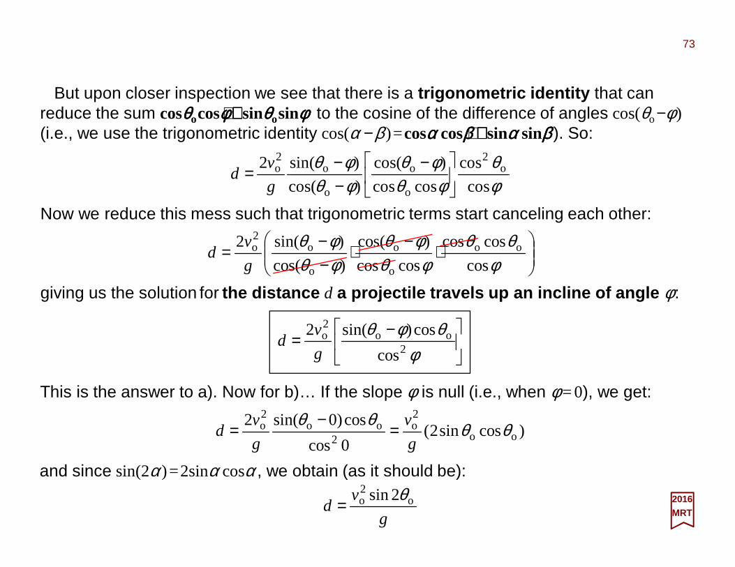
But upon closer inspection we see that there is a trigonometric identity that can reduce the sum cosθθθθocosφφφφ ++++sinθθθθosinφφφφ to the cosine of the difference of angles cos(θo−φ )(i.e., we use the trigonometric identity cos(α −β )=cosαααα cosββββ ++++sinαααα sinββββ ). So:

giving us the solution for the distance d a projectile travels up an incline of angle φ :

φθ

φθφθ

φθφθ

cos

cos

coscos

)cos(

)cos(

)sin(2 o2

o

o

o

o2o

−−−

=g

vd

Now we reduce this mess such that trigonometric terms start canceling each other:

−=

φθφθ

2oo

2o

cos

cos)sin(2

g

vd

⋅

−⋅

−−

=φ

θθφθ

φθφθφθ

cos

coscos

coscos

)cos(

)cos(

)sin(2 oo

o

o

o

o2o

g

vd

This is the answer to a). Now for b)… If the slope φ is null (i.e., when φ= 0), we get:

)cossin2(0cos

cos)0sin(2oo

2o

2oo

2o θθθθ

g

v

g

vd =

−=

and since sin(2α)=2sinα cosα , we obtain (as it should be):

g

vd o

2o 2sin θ

= 2016MRT

73

Now that we have an expression for d, we can find the maximum value of d, called the range , R, by taking the derivative of R=(2vo

2/g)[sin(θ −φ )cosθ /cos2φ ] (remembering that φis a constant) with respect to the angle θ (not θo explicitly) and setting that equal to zero and solving for the angle θ and then evaluating R for that value of θ:

θθφθ

φθθφθ

φθφθ

φθθ d

d

g

v

d

d

g

v

g

v

d

d

d

Rd ]cos)[sin(

cos

2]cos)[sin(

cos

2cos)sin(

cos

22

2o

2

2o

2

2o −⋅=−=

−=

Now the derivative of sin(θ −φ )cosθ with respect to θ is:

θφθθφθθφθθφθθ

θφθθθ

φθθφθθ

sin)sin(cos)cos()sin()sin(cos)cos(

][cos)sin(cos

)][sin(]cos)[sin(

−−−=−⋅−+⋅−=

⋅−+⋅−=⋅−d

d

d

d

d

d

where we have used the product rule d(u⋅v)/dx=u⋅dv/dx+v⋅du/dx (e.g., for u=sin(θ −φ )and v=cosθ ). Using the trigonometric identity cos(α +β )=cosα cosβ −sinα sinβ (for α=θ −φand β=θ ), we get:

)2cos(])cos[(]cos)[sin( φθθφθθφθθ

−=+−=−d

d

which gives us the result:

)2cos(cos

22

2o φθ

φθ−=

g

v

d

Rd2016MRT

74

Now, set dR/dθ = 0 (this provides THE way to find the maximum):

0)2cos(cos

22

2o =−= φθ

φθ g

v

d

Rd

For this to happen (i.e., dR/dθ = 0) we need cos(2θ −φ )= 0 since vo2, g and cosφ are non-

zero. We plot the function y=cosx next and look for a value that corresponds to cosx= 0:

We see that the curve crosses over at π /2 or 90°. This means that cos(π /2)= 0 so 2θ −φ =π /2 or 2θ −φ =90°. This gives us an equation to solve for θ : θ =90°/2+φ /2=45°+φ /2. You will notice that this is consistent with the maximum horizontal range occurring for θ o=45° for φ =0… the answer to the first part of b) (i.e., what value of θo is d a maximum).

Now we must evaluate R for θ =45°+ φ /2:

φ

φφ

φ

φφφ

2

2o

2

2o

cos

245cos

245sin

2

cos

245cos

245sin

2

+

−=

+

−

+=

g

v

g

vR

We must now look for a way to simplify this sin(45°−φ /2)cos(45°+φ /2) monster!

2016MRT

y = cosx y= sinx y= sinx/cosx= tanx

75

π /2

Again, using the trigonometric identities sin(α −β )=sinα cosβ −cosα sinβ and cos(α +β )=cosα cosβ −sinα sinβ we find sin(45°− φ /2)=sin45°cosφ /2 −cos45° sinφ /2=(1/√2)(cosφ /2 −sinφ /2) and cos(45°+ φ /2)=cos45°cosφ /2 −sin45°sinφ /2=(1/√2)(cosφ /2−sinφ /2) so that the product sin(45°−φ /2)cos(45°+φ /2)=½(cosφ /2 −sinφ /2)(cosφ /2−sinφ /2) becomes:

−

+=

+−=

+

−2

sin2

cos22

sin2

cos2

1

2sin

2sin

2cos2

2cos

2

1

245cos

245sin 2222 φφφφφφφφφφ

But since cos2α +sin2α =1 and sin(2α )=2sinα cosα (here with α =φ /2 for both), we obtain:

)sin1(2

1

22sin)1(

2

1

245cos

245sin φφφφ −=

−=

+

−

If we put this back into R=(2vo2/g)[sin(45°−φ /2)cos(45°+φ /2)], we get:

φφ

2

2o

cos

)sin1(½2 −=g

vR

and crossing out the factor of 2 with its fraction (i.e., the ½ factor) gives us our final result:

−=φφ

2

2o

cos

sin1

g

vR

This is the answer to the second part of b) (i.e., What is that maximum value of d?). When the incline angle φ is zero, we’re back to a horizontal range problem. This expression reduces to R=vo

2/g as it should.

2016MRT

76

2016MRT

77Appendix

PART II – MODERN PHYSICSCharge and Current DensitiesElectromagnetic InductionElectromagnetic PotentialsGauge InvarianceMaxwell’s EquationsFoundations of Special RelativityTensors of Rank One4D Formulation of ElectromagnetismPlane Wave Solutions of the Wave

EquationSpecial Relativity and

ElectromagnetismThe Special Lorentz TransformationsRelativistic KinematicsTensors in GeneralThe Metric TensorThe Problem of Radiation in

EnclosuresThermodynamic Considerations

The Wien Displacement LawThe Rayleigh-Jeans LawPlanck’s Resolution of the ProblemPhotons and ElectronsScattering ProblemsThe Rutherford Cross-SectionBohr’s ModelFundamental Properties of WavesThe Hypothesis of de Broglie and EinsteinAppendix: The General Theory of

RelativityReferences

We list here, as a reference, the Contents of the remaining parts of this 10-PART Serieswhich as a whole makes for quite a thorough review of Theoretical Physics (N.B., Since Superstring Theory is still being developed, this content is accurate up to year 1990-ish).

78

PART III – QUANTUM MECHANICSIntroductionSymmetries and ProbabilitiesAngular MomentumQuantum BehaviorPostulatesQuantum Angular MomentumSpherical HarmonicsSpin Angular MomentumTotal Angular MomentumMomentum CouplingGeneral PropagatorFree Particle PropagatorWave PacketsNon-Relativistic ParticleAppendix: Why Quantum? References

2016MRT

PART IV – QUANTUM FIELDSReview of Quantum MechanicsGalilean InvarianceLorentz InvarianceThe Relativity PrinciplePoincaré TransformationsThe Poincaré AlgebraLorentz Transformations

Lorentz Invariant ScalarKlein-Gordon & Dirac

One-Particle StatesWigner’s Little GroupNormalization Factor

Mass Positive-DefiniteBoosts & RotationsMass Zero

The Klein-Gordon EquationThe Dirac EquationReferences

79

2016MRT

80

PART V – THE HYDROGEN ATOMWhat happens at 10−−−−10 m?The Hydrogen AtomSpin-Orbit CouplingOther Interactions

Magnetic & Electric FieldsHyperfine Interactions

Multi-Electron Atoms and MoleculesAppendix – Interactions

The Harmonic OscillatorElectromagnetic InteractionsQuantization of the Radiation FieldTransition ProbabilitiesEinstein’s Coefficients Planck’s LawA Note on Line BroadeningThe Photoelectric EffectHigher Order Electromagnetic Interactions

References2016MRT

81

PART VI – GROUP THEORYSymmetry Groups of PhysicsBasic Definitions and Abstract Vectors Matrices and Matrix MultiplicationSummary of Linear Vector SpacesLinear TransformationsSimilarity TransformationsDual Vector SpacesAdjoint Operator and Inner ProductNorm of a Vector and OrthogonalityProjection, Hermiticity and UnitarityGroup RepresentationsRotation Group SO(2)Irreducible Representation of SO(2)Continuous Translational GroupConjugate Basis VectorsDescription of the Group SO(3)Euler Angles α, β & γGenerators and the Lie AlgebraIrreducible Representation of SO(3)

Particle in a Central FieldTransformation Law for Wave FunctionsTransformation Law for OperatorsRelationship Between SO(3) and SU(2)Single Particle State with SpinEuclidean Groups E2 and E3Irreducible Representation MethodUnitary Irreducible Representation of E3Lorentz and Poincaré GroupsHomogeneous Lorentz TransformationsTranslations and the Poincaré GroupGenerators and the Lie AlgebraRepresentation of the Poincaré GroupNormalization of Basis StatesWave Functions and Field OperatorsRelativistic Wave EquationsGeneral Solution of a Wave EquationCreation and Annihilation OperatorsReferences

2016MRT

82

PART VII–QUANTUM ELECTRODYNAMICSParticles and FieldsSecond QuantizationYukawa PotentialComplex Scalar FieldNoether’s TheoremMaxwell’s EquationsClassical Radiation FieldQuantization of Radiation OscillatorsKlein-Gordon Scalar FieldCharged Scalar FieldPropagator TheoryDirac Spinor FieldQuantizing the Spinor FieldWeyl NeutrinosRelativistic Quantum MechanicsQuantizing the Maxwell FieldCross Sections and the Scattering MatrixPropagator Theory and Rutherford

ScatteringTime Evolution OperatorFeynman’s RulesThe Compton EffectPair AnnihilationMøller ScatteringBhabha ScatteringBremsstrahlungRadiative CorrectionsAnomalous Magnetic MomentInfrared DivergenceLamb ShiftOverview of Renormalization in QEDBrief Review of Regularization in QEDAppendix I: Radiation GaugeAppendix II: Path IntegralsAppendix III: Dirac MatricesReferences

2016MRT

83

Fermion Masses and CouplingsWhy Go Beyond the Standard Model?Grand Unified Theories General Consequences of Grand

UnificationPossible Choices of the Grand Unified

GroupGrand Unified SU(5)Spontaneous Symmetry Breaking in

SU(5)Fermion Masses AgainHierarchy ProblemHiggs Scalars and the Hierarchy

ProblemAppendixReferences

PART VIII – THE STANDARD MODELThe ParticlesThe ForcesThe HadronsScatteringField EquationsFermionsParticle PropagatorsNoether’s Theorem and Global InvarianceLocal Gauge Invariance in QEDYang-Mills Gauge TheoriesQuantum Chromodynamics (QCD)RenormalizationStrong Interactions and Chiral SymmetrySpontaneous Symmetry Breaking (SSB)Weak InteractionsThe SU(2)⊗U(1) Gauge TheorySSB in the Electroweak ModelGauge Boson MassesGauge Boson Mixing and Coupling

2016MRT

84

PART IX – SUPERSYMMETRYMotivationIntroduction to SupersymmetryThe SUSY AlgebraRealizations of the SUSY AlgebraThe Wess-Zumino ModelLagrangian with Mass and Interaction

TermsThe Superpotential Supersymmetric Gauge TheorySpontaneous Breaking of

Supersymmetry F-type SUSY BreakingD-type SUSY BreakingThe Scale of SUSY BreakingThe SUSY Particle SpectrumSupersymmetric Grand UnificationGeneral RelativityThe Principle of EquivalenceGeneral Coordinates

Local Lorentz FramesLocal Lorentz TransformationsGeneral Coordinate TransformationsCovariant DerivativeThe Einstein LagrangianThe Curvature TensorThe Inclusion of MatterThe Newtonian LimitLocal SupersymmetryA Pure SUGRA LagrangianCoupling SUGRA to Matter and Gauge

FieldsHigher-dimensional Theories CompactificationThe Kaluza Model of ElectromagnetismNon-Abelian Kaluza-Klein TheoriesKaluza-Klein Models and the Real WorldN=1 SUGRA in Eleven DimensionsReferences

2016MRT

85

2016MRT

PART X – SUPERSTRING THEORYA History of the Origins of String

TheoriesThe Classical Bosonic StringThe Quantum Bosonic StringThe Interacting StringFermions in String TheoriesString Quantum NumbersAnomaliesThe Heterotic StringCompactification and N=1 SUSYCompactification and Chiral FermionsCompactification and Symmetry

BreakingEpilogue: Quantum GravityAppendix I: Feynman’s Take on

GravitationAppendix II: Review of SupersymmetryAppendix III: A Brief Review of Groups

and Forms

Appendix IV: The Gamma FunctionAppendix V: The Beta FunctionReferences

2016MRT

References 86

M. Klein, Calculus , 2-nd Edition, Dover, 1977. New York UniversityBelieve it or not, my father had the first edition in 2 volumes and when I found them and browsed through them I was amazed at the Motion in One Dimension in a Resisting Medium part which eventually ended up being the case for this treatment of air resistance in ballistic problems. Since then, I’ve always enjoyed Klein’s way of presenting calculus using physical concepts. The only problemthough is his use of 32 [ft/sec] everywhere! Most of the gravitation discussion related to hollow or filled up spheres is from this book.H. Benson, University Physics , Revised Edition, 1996. Vanier College Amazing course which is somewhat similar to the one I had with Halliday and Resnick back in 1986-88. It is a great page turner with special topics everywhere. The problems in themselves are worth solving (e.g., kinematics of a basketball shot!) and many have an equation to prove that is actually displayed! My edition has 44 chapters spread across 942 pages covering everything from vectors, kinematics, inertia, particle dynamics, work and energy, conservation of energy, momentum, rotations about a fixed axis, gravitation, solids and fluids, oscillations, waves and sound, temperature and the ideal gas law, thermodynamics and entropy, electrostatics, the electric field, pretty much everything ‘electric and magnetic’, Maxwell’s equations, light and optics, special relativity , quantum theory and wave mechanics, atoms and solids. Finally nuclear physics and elementary particles and a (1997) view of Grand Unified Theory. C. Harper, Introduction to Mathematical Physics , Prentice Hall, 1976.California State University, Haywood This is my favorite go-to reference for mathematical physics. Most of the differential equations presentation and solutions, complex variable and matrix definitions, and most of his examples and problems, &c. served as the primer for this work. Harper’s book is so concise that you can pretty much read it in about 2 weeks and the presentation is impeccable for this very readable 300 page mathematical physics volume. D.G. Zill, W. S. Wright, Advanced Engineering Mathematics , 4-th Edition, Jones & Bartlett, 2011. Loyola Mary-mount UniversityIf you are going to go into some scientific field that makes you learn engineering physics you should get this book as a reference. Besides being set in color, it is easily readable and with just enough conceptual ‘meat’ around the physical ‘bone’ to capture your attention without being to mathematical about it. I mean, when I browsed through it I wished I had used this book for my course!F. P. Beer, E. R. Johnson, W. E. Clausen, Vector Mechanics for Engineers , Volume II - Dynamics, 8-Edition, McGraw-Hill, 2007. Lehigh University, University of Connecticut, Ohio State UniversityGreat reference and a constant page turner with amazing color graphics. It is fairly advanced though but requires some study.T. Allen Jr, R.L. Ditsworth, Fluid Mechanics , McGraw Hill, 1972. College of Engineering Sciences at Arizona State UniversityMy father’s book. I first skimmed through this book when I was 14 and fell in love with it instantly. The fluid mechanics here is all theirs. W.J. Thomson, Introduction to Space Dynamics , Dover, 1986. University of California at Santa BarbaraGreat introduction to vectors, kinematics, dynamics and earth & satellite-related applications. Most of the mathematical treatment for kinematics, rotation transformations and satellite or ballistic dynamics here is based on this book since it is succinct and to the point.

−1+1

ei ej

p=2n=1

Spinor on the circle

y

x

rd

C

0.5 1.0 1.5

r

(a,b)

(x,y)•

222

2 7854.04

π

2ππ

π2

ddd

r

rC

≅=

==

=

Area

222 )()( rbyax =−+−

Parametric equation

222

2π

ryx

r

=+

= AreaCircle

≠−+∈=−

∈=+=

jiee

npiji

piji

ee

ji

ji ),...,1(,1

),...,1(,1