part 2: sparrow users guide - usgs · part 2: sparrow users guide 2.1 introduction part 2 documents...
TRANSCRIPT
Part 2: SPARROW Users Guide
2.1 Introduction Part 2 documents operation of the SPARROW model program, including preparing the model input data
set, executing the model program, interpreting model output, and diagnosing execution errors. The material in this part of the documentation builds on information presented in Part 1; therefore discussions of operation frequently refer back to specific sections in Part 1. Conversely, the description of model operations presented in this part of the documentation, and experience with executing the model or viewing model output, may enhance understanding of the concepts provided in Part 1. For example, the reader may find that viewing the input data file as instructed in section 2.6.1, “Data file,” aids in understanding the material presented in section 1.3.2 of Part 1, “Stream network topology.”
Most components of the SPARROW modeling process are accessible with knowledge of basic statistical concepts (such as hypothesis testing, statistical regression modeling) and basic knowledge of the Base Statistical Analysis System (SAS) software (Statistical Analysis System Institute, 2000a), and this documentation assumes such knowledge. Certain model applications discussed in this chapter (for example, complex process specification and bootstrap analysis) require more advanced statistical background, or some knowledge of SAS Interactive Matrix Language (SAS/IML) and programming; sections containing discussion of these applications are marked ‘advanced’. The user interested in the basic components of SPARROW modeling may wish to focus attention away from these ‘advanced’ sections, returning to them after gaining facility with basic operation of the model program.
2.2 System requirements The SPARROW model code is written in SAS Macro Language, with statistical procedures written in the
SAS IML. SPARROW version 2.1 runs with SAS version 8.0 (or higher), supported on Windows 95 or Windows NT Version 4.0 (or higher). Consult SAS documentation (for example, Statistical Analysis System Institute, 2000a) for additional information about SAS software. SPARROW model execution requires SAS software components Base SAS, the SAS statistical procedures (SAS/STAT) and SAS/IML. The SAS Geographic Information System (SAS/GIS) software component is optional for producing maps of model output. The minimum hardware configuration is Intel or Intel-compatible Pentium class processor with 64 megabytes of memory, and XGA or SVGA monitors with minimum screen resolution of 800x600. The work directory used by the SAS system must be of sufficient capacity to hold files as large as several hundred megabytes.
A basic knowledge of the Base SAS software is required to develop simple SPARROW models; modifications to the model code in order to develop more complex models require more detailed knowledge of SAS/IML language and programming (Statistical Analysis System Institute, 2000b).
2.3 Obtaining and Installing Software The following steps are needed to obtain and install the SPARROW model software:
1. Obtain the SPARROW software files through the internet by accessing the U.S. Geological Survey Water Resources Applications Software page (http://water.usgs.gov/software/) and selecting Surface Water and SPARROW. Follow the instructions for downloading the compressed file “sparrow_package_v2.zip.”
2. Select a base directory (for example, the host root directory) in which to establish the SPARROW directory tree to house the model and data. From this directory, create the directory “base-directory_name\sparrow” and extract the compressed file “sparrow_package_v2.zip.” The extraction creates four subdirectories (fig. 2.1):
“\master” - contains the model program files “\data” - contains the model input data set “\results” - contains the model output files (data tables and graphs) from each run “\gis” (optional) - contains the SAS/GIS mapfiles and layers used to produce SAS/GIS maps of model output. The “.\sparrow\master” subdirectory contains all the software (SAS programs, dynamically linked library (DLL) files, and FORTRAN code) required to run the model. Additional files are included to assist in building an input data file, to provide advice in creating GIS coverages and DLL files, and to document

The SPARROW Surface Water-Quality Model: Theory, Application and User Documentation 124
changes in the current SPARROW version. The “.\sparrow\data” subdirectory contains an input data set (“sparrow_data1”) corresponding to a national example application, and the “.\sparrow\results” subdirectory contains an example control file (“sparrow_control_example”) for a model application that will demonstrate executing the model and viewing output. The “.\sparrow\gis” subdirectory contains GIS coverages for implementing the national example application. The directory is optional, however, pending the user’s inclusion of geographic information system mapping features in his/her SPARROW application.
3. Modify the host PC system search paths so that the DLL code used by the SPARROW program, specifically the files “sparrow.dll” and “lf90wiod.dll,” will work on your machine. This is accomplished by modifying the Path command in the PC system settings so that it includes the pathname for the directory (“base-directory_name”\sparrow\master) containing the SPARROW model program files. [Note, this step is optional as SPARROW can successfully run, albeit slower, without the DLL, but see discussion of the variable if_accumulate_with_dll in section 2.6.3.7, “Options for model execution.”]
a. Click Start, and select Settings, Control Panel; double-click the System icon to open the System Properties window.
b. Click the Advanced tab and select Environment Variables. In the System variables field, double-click the variable Path from the listbox to edit it. At the end of this line, enter a semi-colon followed by the full path in which the SPARROW program resides (e.g. if the root directory of the d: drive is selected for the base directory, enter “D:\sparrow\master” at the end of this line). This step may require system administrator permission to execute successfully.
c. Click OK to exit and store the modification. ***** Note that your PC must be rebooted for the change to take effect.*****

Part 2: SPARROW User’s Guide 125
Figure 2.1. SPARROW directory structure.
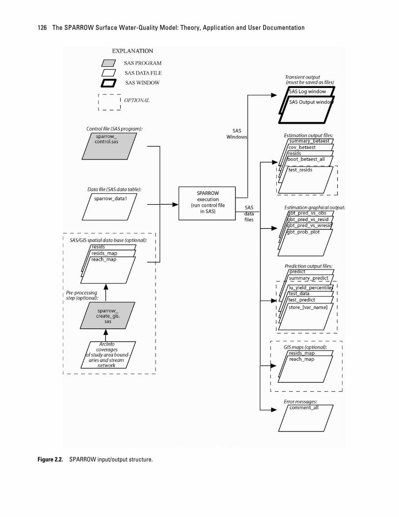
2.4 Input/output structure The input/output structure of SPARROW is shown in figure 2.2. For a typical SPARROW application, the
user modifies only the control file and/or the data file.
The SPARROW Surface Water-Quality Model: Theory, Application and User Documentation 126
Figure 2.2. SPARROW input/output structure.
Part 2: SPARROW User’s Guide 127
Data for all input variables are contained within a single input data file, a SAS data set (specifically, data table). The SAS file “sparrow_data1,” downloaded from the SPARROW software web site (installed in the “.\sparrow\data” directory), is an example input data file. This data file contains one record for each stream reach in the modeled river basin, with data for characteristics of the reach and its associated incremental watershed. See section 2.6.1, “Data file,” for additional discussion. For SPARROW to run correctly, it is necessary that the data file contain a variable that permits ordering the observations in downstream hydrologic order.
The control file is a SAS program file containing commands that identify the data to be used, the variables to be included in the analysis, the model form, and the selection of options for model execution (described in detail in section 2.6.3, “Control file,”). The SAS program “sparrow_control_example.sas”, downloaded from the SPARROW software web page (installed in the “.\sparrow\results” directory), is an example control file. The user typically edits this file before each model run, for example to change a feature in the model structure or to specify a change in the procedure for estimating model coefficients, and saves the edited file using a descriptive or catalog name that identifies the model run. (For example, the name “TN_2.sas” might represent the control file for modeling total nitrogen, specifying the model structure, and selecting the variables catalogued as model number 2). To facilitate retrieval of results from a specific model run, create a subdirectory in “sparrow\results” to contain the modified control file along with the output files from the execution.
Execution of a SPARROW model produces four types of output: messages to the SAS Log window, results listed in the SAS Output window and referred to as “output listing”, text files that summarize current and previous model specifications and estimation results, and SAS data files (data tables and graphs) written to the directory “.\sparrow\results.” Optionally, certain data files can be linked to SAS/GIS data sets. The log and output listing and SAS data files are described in detail in section 2.8, “Model output.” The SAS data files should be moved, after model execution, from the “.\sparrow\results” directory to more permanent storage in another directory (for example, a subdirectory created to store the results from this particular model, along with the control file), otherwise they could be lost when subsequent model execution overwrites them. In addition, the results listed in the SAS Log and Output windows must be saved (as .log and .lst files, respectively) to retain a permanent record. Note that SPARROW retains all results from the most previous run by attaching the prefix BAK_ to the name of any results file in the results directory; however, any existing backup results files are overwritten by this procedure.
2.5 Navigating in SAS for Windows This introduction to basic features of navigating in the SAS for Windows environment is intended for
experienced SAS users who have worked in SAS on operating systems other than Windows.
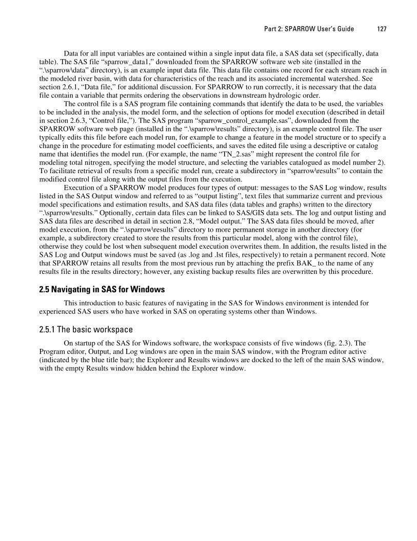
2.5.1 The basic workspace On startup of the SAS for Windows software, the workspace consists of five windows (fig. 2.3). The
Program editor, Output, and Log windows are open in the main SAS window, with the Program editor active (indicated by the blue title bar); the Explorer and Results windows are docked to the left of the main SAS window, with the empty Results window hidden behind the Explorer window.
The SPARROW Surface Water-Quality Model: Theory, Application and User Documentation 128
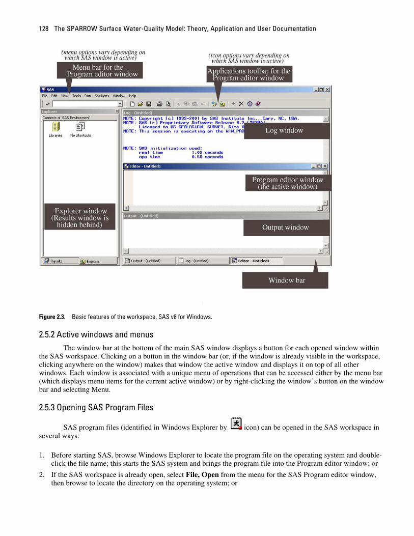
Figure 2.3. Basic features of the workspace, SAS v8 for Windows.
2.5.2 Active windows and menus The window bar at the bottom of the main SAS window displays a button for each opened window within
the SAS workspace. Clicking on a button in the window bar (or, if the window is already visible in the workspace, clicking anywhere on the window) makes that window the active window and displays it on top of all other windows. Each window is associated with a unique menu of operations that can be accessed either by the menu bar (which displays menu items for the current active window) or by right-clicking the window’s button on the window bar and selecting Menu.
2.5.3 Opening SAS Program Files
SAS program files (identified in Windows Explorer by icon) can be opened in the SAS workspace in several ways:
1. Before starting SAS, browse Windows Explorer to locate the program file on the operating system and double-click the file name; this starts the SAS system and brings the program file into the Program editor window; or
2. If the SAS workspace is already open, select File, Open from the menu for the SAS Program editor window, then browse to locate the directory on the operating system; or
Part 2: SPARROW User’s Guide 129
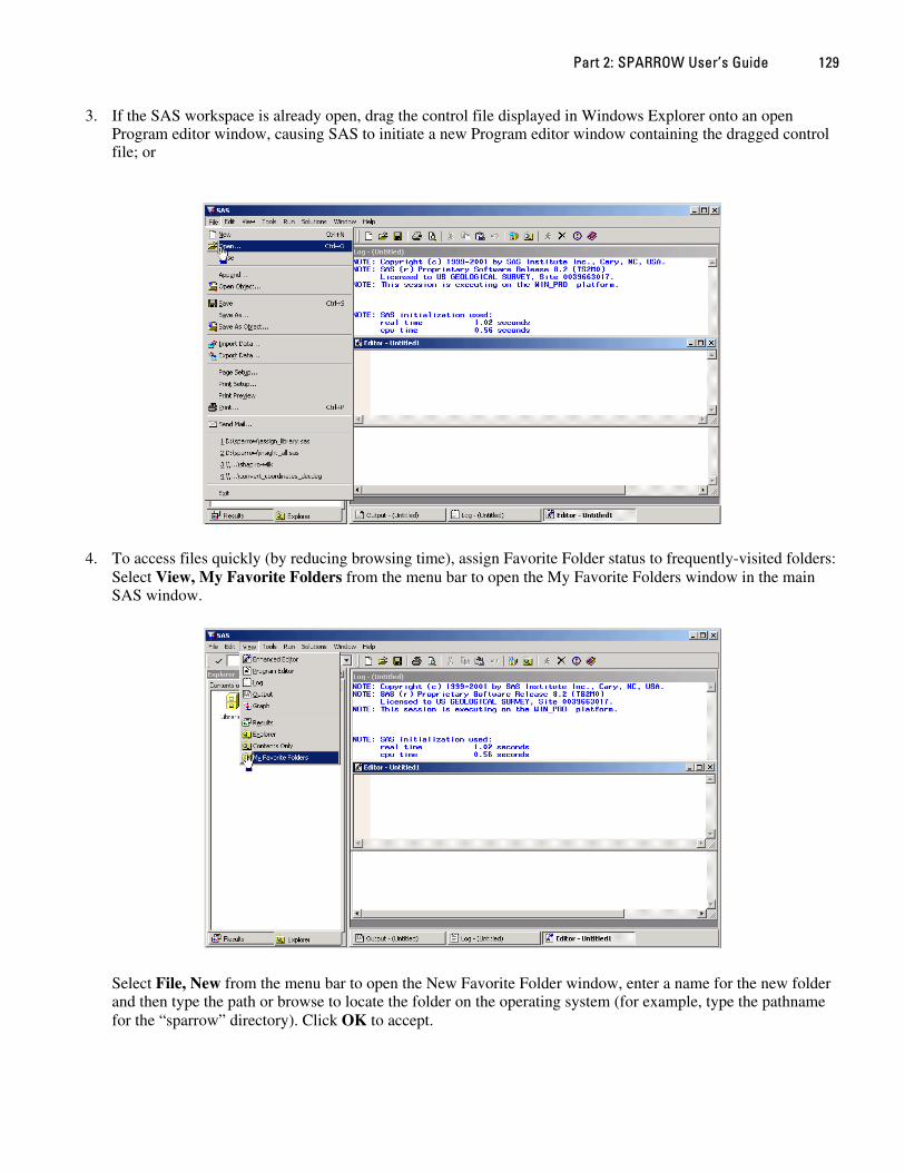
3. If the SAS workspace is already open, drag the control file displayed in Windows Explorer onto an open Program editor window, causing SAS to initiate a new Program editor window containing the dragged control file; or
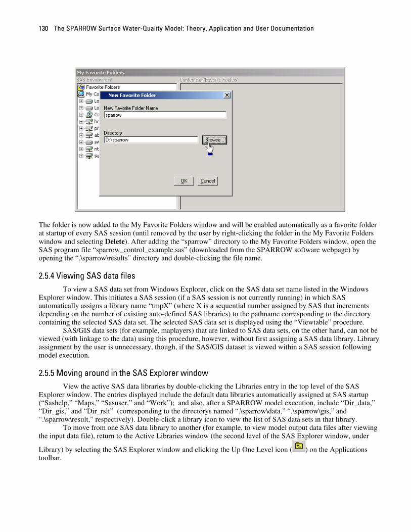
4. To access files quickly (by reducing browsing time), assign Favorite Folder status to frequently-visited folders: Select View, My Favorite Folders from the menu bar to open the My Favorite Folders window in the main SAS window.
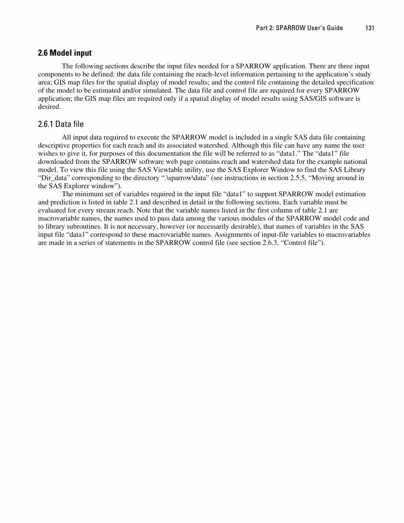
Select File, New from the menu bar to open the New Favorite Folder window, enter a name for the new folder and then type the path or browse to locate the folder on the operating system (for example, type the pathname for the “sparrow” directory). Click OK to accept.
The SPARROW Surface Water-Quality Model: Theory, Application and User Documentation 130
The folder is now added to the My Favorite Folders window and will be enabled automatically as a favorite folder at startup of every SAS session (until removed by the user by right-clicking the folder in the My Favorite Folders window and selecting Delete). After adding the “sparrow” directory to the My Favorite Folders window, open the SAS program file “sparrow_control_example.sas” (downloaded from the SPARROW software webpage) by opening the “.\sparrow\results” directory and double-clicking the file name.
2.5.4 Viewing SAS data files To view a SAS data set from Windows Explorer, click on the SAS data set name listed in the Windows
Explorer window. This initiates a SAS session (if a SAS session is not currently running) in which SAS automatically assigns a library name “tmpX” (where X is a sequential number assigned by SAS that increments depending on the number of existing auto-defined SAS libraries) to the pathname corresponding to the directory containing the selected SAS data set. The selected SAS data set is displayed using the “Viewtable” procedure.
SAS/GIS data sets (for example, maplayers) that are linked to SAS data sets, on the other hand, can not be viewed (with linkage to the data) using this procedure, however, without first assigning a SAS data library. Library assignment by the user is unnecessary, though, if the SAS/GIS dataset is viewed within a SAS session following model execution.
2.5.5 Moving around in the SAS Explorer window View the active SAS data libraries by double-clicking the Libraries entry in the top level of the SAS
Explorer window. The entries displayed include the default data libraries automatically assigned at SAS startup (“Sashelp,” “Maps,” “Sasuser,” and “Work”); and also, after a SPARROW model execution, include “Dir_data,” “Dir_gis,” and “Dir_rslt” (corresponding to the directorys named “.\sparrow\data,” “.\sparrow\gis,” and “.\sparrow\result,” respectively). Double-click a library icon to view the list of SAS data sets in that library.
To move from one SAS data library to another (for example, to view model output data files after viewing the input data file), return to the Active Libraries window (the second level of the SAS Explorer window, under
Library) by selecting the SAS Explorer window and clicking the Up One Level icon ( ) on the Applications toolbar.
Part 2: SPARROW User’s Guide 131
2.6 Model input The following sections describe the input files needed for a SPARROW application. There are three input
components to be defined: the data file containing the reach-level information pertaining to the application’s study area; GIS map files for the spatial display of model results; and the control file containing the detailed specification of the model to be estimated and/or simulated. The data file and control file are required for every SPARROW application; the GIS map files are required only if a spatial display of model results using SAS/GIS software is desired.
2.6.1 Data file All input data required to execute the SPARROW model is included in a single SAS data file containing
descriptive properties for each reach and its associated watershed. Although this file can have any name the user wishes to give it, for purposes of this documentation the file will be referred to as “data1.” The “data1” file downloaded from the SPARROW software web page contains reach and watershed data for the example national model. To view this file using the SAS Viewtable utility, use the SAS Explorer Window to find the SAS Library “Dir_data” corresponding to the directory “.\sparrow\data” (see instructions in section 2.5.5, “Moving around in the SAS Explorer window”).
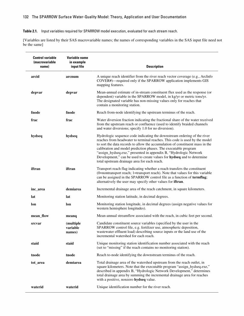
The minimum set of variables required in the input file “data1” to support SPARROW model estimation and prediction is listed in table 2.1 and described in detail in the following sections. Each variable must be evaluated for every stream reach. Note that the variable names listed in the first column of table 2.1 are macrovariable names, the names used to pass data among the various modules of the SPARROW model code and to library subroutines. It is not necessary, however (or necessarily desirable), that names of variables in the SAS input file “data1” correspond to these macrovariable names. Assignments of input-file variables to macrovariables are made in a series of statements in the SPARROW control file (see section 2.6.3, “Control file”).
The SPARROW Surface Water-Quality Model: Theory, Application and User Documentation 132
Table 2.1. Input variables required for SPARROW model execution, evaluated for each stream reach. [Variables are listed by their SAS macrovariable names; the names of corresponding variables in the SAS input file need not be the same]
Control variable (macrovariable
name)
Variable name in example input file Description
arcid arcnum A unique reach identifier from the river reach vector coverage (e.g., ArcInfo COVER#)—required only if the SPARROW application implements GIS mapping features.
depvar depvar Mean-annual estimate of in-stream constituent flux used as the response (or dependent) variable in the SPARROW model, in kg/yr or metric tons/yr. The designated variable has non-missing values only for reaches that contain a monitoring station.
fnode fnode Reach from-node identifying the upstream terminus of the reach.
frac frac Water diversion fraction indicating the fractional share of the water received from the upstream reach or confluence (used to identify braided channels and water diversions; specify 1.0 for no diversion).
hydseq hydseq Hydrologic sequence code indicating the downstream ordering of the river reaches from headwater to terminal reaches. This code is used by the model to sort the data records to allow the accumulation of constituent mass in the calibration and model prediction phases. The executable program “assign_hydseq.exe,” presented in appendix B, “Hydrologic Network Development,” can be used to create values for hydseq and to determine total upstream drainage area for each reach.
iftran iftran Transport reach flag indicating whether a reach transfers the constituent (0=nontransport reach; 1=transport reach). Note that values for this variable can be assigned in the SPARROW control file as a function of termflag; alternatively the user may specify other values for iftran.
inc_area demiarea Incremental drainage area of the reach catchment, in square kilometers.
lat lat Monitoring station latitude, in decimal degrees.
lon lon Monitoring station longitude, in decimal degrees (assign negative values for western hemisphere longitudes).
mean_flow meanq Mean-annual streamflow associated with the reach, in cubic feet per second.
srcvar (multiple variable names)
Candidate constituent source variables (specified by the user in the SPARROW control file, e.g. fertilizer use, atmospheric deposition, wastewater effluent load) describing source inputs or the land use of the incremental watershed for each reach.
staid staid Unique monitoring station identification number associated with the reach (set to “missing” if the reach contains no monitoring station).
tnode tnode Reach to-node identifying the downstream terminus of the reach.
tot_area demtarea Total drainage area of the watershed upstream from the reach outlet, in square kilometers. Note that the executable program “assign_hydseq.exe,” described in appendix B, “Hydrologic Network Development,” determines total drainage area by summing the incremental drainage area for reaches with a positive, nonzero hydseq value.
waterid waterid Unique identification number for the river reach.
Part 2: SPARROW User’s Guide 133
2.6.1.1 Reach topology
A digital vector- or raster-based stream network with verified node topology serves as the model infrastructure to support water and contaminant routing in streams and reservoirs and to spatially reference reach and watershed properties in the SPARROW model. The network of stream reaches must have a standard node topology with proper hydrologic connections between reaches. Upstream and downstream nodes must be uniquely identified according to the numerical values in fnode and tnode, respectively (see table 2.1). Each reach is assigned a unique identification number in waterid. The numbering system for both the nodes and the reach identification variables should be compact, meaning that the assigned numbering sequence should not contain many gaps. This is a technical requirement that is necessary in order to facilitate the referencing of reaches in a dense data matrix—one that conserves memory by not having many rows containing no data. If SAS/GIS is to be used to display SPARROW results, a second identification number, arcid, must be defined to correspond to the internal ARC “cover-id”—see appendix C, “SAS/GIS Mapfile Creation.” Reaches must also be hydrologically oriented in the direction of flow (i.e., downstream ordering from headwater to terminal reaches) according to a unique numerical sequence number that is assigned to each reach and identified in the variable hydseq. The user can create values of hydseq by executing the program “assign_hydseq.exe” (see appendix B, “Hydrologic Network Development” for details). Stream braiding and water diversions can exist in the network, provided estimates of the fraction of water diverted can be determined; this fraction must be placed in the field frac (see table 2.1). The variable iftran controls the gross transport properties of a reach, taking a value of 0 if the reach has no mean flow or is a coastal reach that has no transport, or a value of 1 if any flux is transported through the reach to the downstream segment.
2.6.1.2 Reach attributes
River reach properties should include mean streamflow (mean_flow), incremental drainage area (inc_area), and total drainage area (tot_area). The executable program “assign_hydseq.exe,” presented in appendix B, “Hydrologic Network Development,” can be used to determine incremental and total drainage area for each reach. Additionally, every SPARROW model must include at least one source variable; the list of source variables included in the model are referenced by the control variable srcvar. The example SPARROW application for total nitrogen included with the model software specifies five source variables: point, atmdep, fertilizer, waste, and nonagr, corresponding to point sources, atmospheric deposition, fertilizer application, animal waste, and non-urban/non-agricultural land.
A number of additional reach attributes, not listed in table 2.1, could be included in the “data1” file to describe reach attenuation processes. Estimates of mean water velocity can be used to estimate in-stream contaminant attenuation as a function of the water time of travel (see section 1.4.4 of Part 1). The example “data1” file for the Reach File 1 (RF1) stream network contains a variable named rchtot, representing the reach average time of travel calculated as the ratio of channel length to mean water velocity, which can be used to evaluate in-stream attenuation processes of the kind described in section 1.4.4 of Part 1 (see section 2.6.3.4 for descriptions of how these processes are specified in the SPARROW control file). If water time-of-travel estimates cannot be determined, in-stream attenuation can be alternatively estimated as a function of channel length (see discussion in section 1.3.1.4 of Part 1). Contaminant attenuation in reservoirs and lakes is estimated in the example SPARROW application (downloaded from the SPARROW sofware web page) as a function of the areal water load (hload, calculated as the ratio of outflow to surface area of the reservoir, is assigned to the outlet reach of the reservoir). The proper application of reach and reservoir decay functions requires the identification of reaches according to a reach-type indicator, rchtype, which identifies a reach as a river reach (unimpounded), as an interior or transport segment of a reservoir, or as an outlet reach of a reservoir.
2.6.1.3 Contaminant flux
Estimates of mean-annual flux for monitoring stations that are spatially referenced to the reach network are stored in the variable depvar. Flux estimates are used as the dependent variable in calibrations of SPARROW models and are determined from the application of load-estimation techniques to long-term stream monitoring station records (see section 1.3.1 of Part 1, “Monitoring station flux estimation,” for details). The standard error of estimation of the mean-annual flux can be used to statistically weight the calibration of the model in cases where errors in flux estimation have a noticeable effect on the variability of SPARROW model residuals. A unique station
The SPARROW Surface Water-Quality Model: Theory, Application and User Documentation 134
identification number, staid, and the geographic coordinates of the monitoring station location (lat, lon) are also required in the input file “data1”.
2.6.2 Geographic Information System (GIS) base maps (optional) Users may create an optional set of map layers in SAS/GIS for the display of model output. Alternatively,
users may export SAS model output files either directly or via text and Dbase files to standard GIS display and analysis packages, such as ArcView or ArcInfo.
Two types of GIS coverages are useful for displaying and interpreting SPARROW output. The first is a base map consisting of water-quality monitoring station locations and a background coverage of political boundaries (e.g., states or counties). This base map is used to display the model prediction residuals for the monitoring station locations. This can assist users in identifying spatial patterns in model residuals that may be indicative of spatial biases in model predictions. For example, if the model consistently over- or under-predicts water-quality loads in a particular region (i.e., negative or positive residuals), this may suggest the presence of one or more watershed properties in this region that influence stream water quality but are not accurately represented in the model specification. On the other hand, absence of geographic patterns in the residuals (i.e., random spatial distribution of residuals) is consistent with a properly specified model.
A second base map consists of the network of river and stream reaches that is used as the SPARROW modeling infrastructure. This map is used primarily to display any of the reach-level predictions that are output from the model (described in section 2.8, “Prediction output”) but may also be useful if it is linked to the variables in the input file “sparrow_data1” to river reaches so that any reach or watershed property contained in the file can be mapped by reach.
To create SAS/GIS layers and mapfiles from these GIS coverages, the user first converts the coverages to Arc export files and imports them to SAS/GIS. Instructions for importing the “.e00” Arc export files using the SAS program “sparrow_create_gis.sas” are given in appendix C, along with instructions for adjusting the display of mapped information.
2.6.3 Control file The core of SPARROW modeling and analysis is the specification of the SPARROW control file. The
control file is a SAS program file containing the commands that run the model. This file consists of a series of statements that identify the data to be used, the variables to be included in the analysis, the model form, and select the options for model execution. The control file is edited (in a text editor of the user’s choice, or in the SAS Program window) before each model run.
The control file downloaded from the SPARROW software web page is specified to estimate the example national model and should serve as a useful template for tailoring a SPARROW analysis. As a visual aid to the following discussion of control-file contents, load the example control file “sparrow_control_example.sas” (in the directory “sparrow/results”) in the SAS Program editor window using procedures described in section 2.5.3, “Opening SAS program files.”
The statements in the control file are in effect assignments of values or variable names to the model control variables (technically, SAS macrovariables). A control variable specification takes the general form:
%let control_variable = response ;
The %let is a SAS macro command telling SAS to create a macro variable having the name control_variable that contains the value given by response. The semicolon after the response terminates the assignment statement. The following discussion addresses the issues to be considered in constructing appropriate responses for each control variable. Examples of appropriate responses will be described in addition to strategies for specifying the analysis to efficiently converge on an acceptable model.
In writing the SPARROW program, every effort has been made to minimize the number of control variables while providing a wide range of flexibility in model specification. A number of control variables address technical elements of the estimation and can be left “as is” in the typical analysis. Other variables allow the user to segment the analysis into a sequence of steps, beginning with debugging a model specification, obtaining an acceptable model form with preliminary predictions, and, finally (with the bootstrap analysis), producing predictions that reflect the full range of uncertainty included in the model.
Part 2: SPARROW User’s Guide 135
It is expected that in most model applications, the desired model functionality and output can be achieved using the standard SPARROW core program code (downloaded from the SPARROW software web page as the set of program files) and therefore can be implemented by modifying the control-variable responses in the control file (as described in the remainder of the sections under 2.6.3). There are, however, certain advanced applications that require modification of the SPARROW core program code and, as such, can not be run from the control file. Because SPARROW is written in open SAS code, with internal documentation describing the purpose of groups of SAS statements in each SPARROW module, such modification is possible. The user is cautioned, however, that detailed guidance for modifying these modules is not provided either in this document or in the current version of internal documentation within the module.
A review of basic conventions of SAS programming language may assist the user in constructing correct responses for the control file variables. First, the text for the response in a %let statement can span one or more lines in the file, with a semicolon terminating the response. In some cases (for example, see section 2.6.3.8, “Data modifications”), the response itself is SAS program code that contains a semicolon as part of the response. In that case, the response must be enclosed within the SAS macro function %str() so that SAS does not interpret the semicolon within the response to be the termination of the response.
Second, a given control variable can be specified within the control file multiple times. Only the last instance of a control variable in the file defines the variable’s operational value. This feature allows the user to retain optional specifications of a control variable within a given control file, modifying the particular analysis being performed by simply copying the desired variable specification to the bottom of a list of alternative specifications.
Third, for control variables designated ‘optional,’ the control variable can be specified to have a null response. That is, the control variable must still be included in the control file but it can be assigned a value of nothing. This is done by immediately following the equal sign in the statement by a semicolon (for example, see the response for the control variable home_gis at the end of the following blocked section).
The control variable specifications in the control file are organized into eight sections corresponding to common elements of the model. The following descriptions of appropriate responses for each of the control variables are divided into sections matching the organization of the control file.
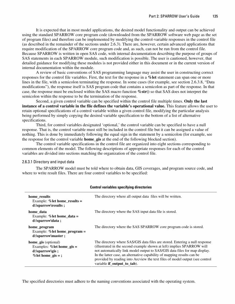
2.6.3.1 Directory and input data The SPARROW model must be told where to obtain data, GIS coverages, and program source code, and
where to write result files. There are four control variables to be specified:
Control variables specifying directories
home_results Example: %let home_results = d:\sparrow\results ;
The directory where all output data files will be written.
home_data Example: %let home_data = d:\sparrow\data ;
The directory where the SAS input data file is stored.
home_program Example: %let home_program = d:\sparrow\master ;
The directory where the SAS SPARROW core program code is stored.
home_gis (optional) Examples: %let home_gis = d:\sparrow\gis ; %let home_gis = ;
The directory where SAS/GIS data files are stored. Entering a null response (illustrated in the second example shown at left) implies SPARROW will not automatically link model output to SAS/GIS data files for map display. In the latter case, an alternative capability of mapping results can be provided by reading into Arcview the text files of model output (see control variable if_output_to_tab).
The specified directories must adhere to the naming conventions associated with the operating system.
The SPARROW Surface Water-Quality Model: Theory, Application and User Documentation 136
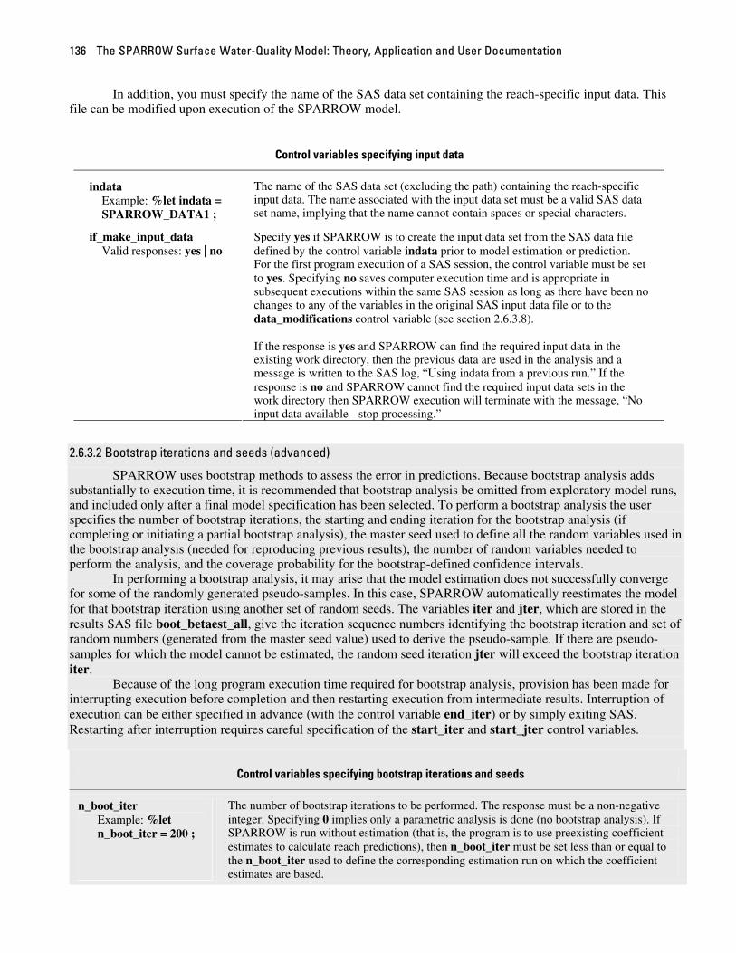
In addition, you must specify the name of the SAS data set containing the reach-specific input data. This file can be modified upon execution of the SPARROW model.
Control variables specifying input data
indata Example: %let indata = SPARROW_DATA1 ;
The name of the SAS data set (excluding the path) containing the reach-specific input data. The name associated with the input data set must be a valid SAS data set name, implying that the name cannot contain spaces or special characters.
if_make_input_data Valid responses: yes | no
Specify yes if SPARROW is to create the input data set from the SAS data file defined by the control variable indata prior to model estimation or prediction. For the first program execution of a SAS session, the control variable must be set to yes. Specifying no saves computer execution time and is appropriate in subsequent executions within the same SAS session as long as there have been no changes to any of the variables in the original SAS input data file or to the data_modifications control variable (see section 2.6.3.8). If the response is yes and SPARROW can find the required input data in the existing work directory, then the previous data are used in the analysis and a message is written to the SAS log, “Using indata from a previous run.” If the response is no and SPARROW cannot find the required input data sets in the work directory then SPARROW execution will terminate with the message, “No input data available - stop processing.”
2.6.3.2 Bootstrap iterations and seeds (advanced)
SPARROW uses bootstrap methods to assess the error in predictions. Because bootstrap analysis adds substantially to execution time, it is recommended that bootstrap analysis be omitted from exploratory model runs, and included only after a final model specification has been selected. To perform a bootstrap analysis the user specifies the number of bootstrap iterations, the starting and ending iteration for the bootstrap analysis (if completing or initiating a partial bootstrap analysis), the master seed used to define all the random variables used in the bootstrap analysis (needed for reproducing previous results), the number of random variables needed to perform the analysis, and the coverage probability for the bootstrap-defined confidence intervals.
In performing a bootstrap analysis, it may arise that the model estimation does not successfully converge for some of the randomly generated pseudo-samples. In this case, SPARROW automatically reestimates the model for that bootstrap iteration using another set of random seeds. The variables iter and jter, which are stored in the results SAS file boot_betaest_all, give the iteration sequence numbers identifying the bootstrap iteration and set of random numbers (generated from the master seed value) used to derive the pseudo-sample. If there are pseudo-samples for which the model cannot be estimated, the random seed iteration jter will exceed the bootstrap iteration iter.
Because of the long program execution time required for bootstrap analysis, provision has been made for interrupting execution before completion and then restarting execution from intermediate results. Interruption of execution can be either specified in advance (with the control variable end_iter) or by simply exiting SAS. Restarting after interruption requires careful specification of the start_iter and start_jter control variables.
Control variables specifying bootstrap iterations and seeds
n_boot_iter Example: %let n_boot_iter = 200 ;
The number of bootstrap iterations to be performed. The response must be a non-negative integer. Specifying 0 implies only a parametric analysis is done (no bootstrap analysis). If SPARROW is run without estimation (that is, the program is to use preexisting coefficient estimates to calculate reach predictions), then n_boot_iter must be set less than or equal to the n_boot_iter used to define the corresponding estimation run on which the coefficient estimates are based.
Part 2: SPARROW User’s Guide 137
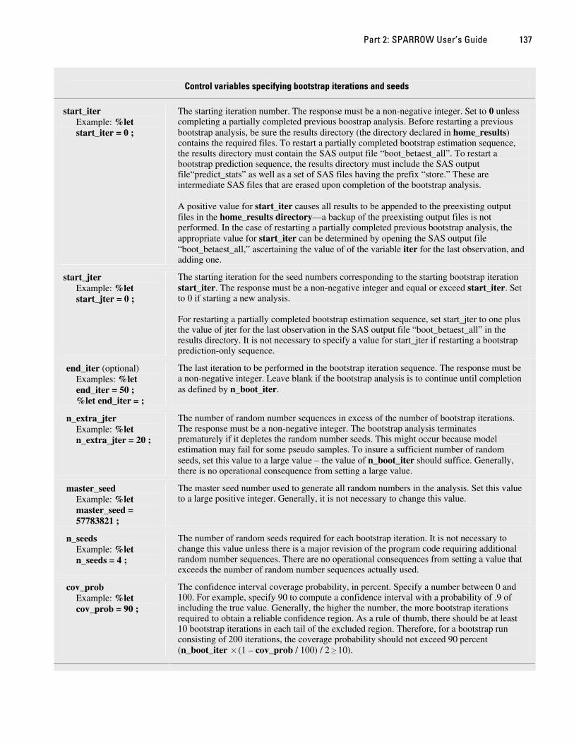
Control variables specifying bootstrap iterations and seeds
start_iter Example: %let start_iter = 0 ;
The starting iteration number. The response must be a non-negative integer. Set to 0 unless completing a partially completed previous boostrap analysis. Before restarting a previous bootstrap analysis, be sure the results directory (the directory declared in home_results) contains the required files. To restart a partially completed bootstrap estimation sequence, the results directory must contain the SAS output file “boot_betaest_all”. To restart a bootstrap prediction sequence, the results directory must include the SAS output file“predict_stats” as well as a set of SAS files having the prefix “store.” These are intermediate SAS files that are erased upon completion of the bootstrap analysis. A positive value for start_iter causes all results to be appended to the preexisting output files in the home_results directory—a backup of the preexisting output files is not performed. In the case of restarting a partially completed previous bootstrap analysis, the appropriate value for start_iter can be determined by opening the SAS output file “boot_betaest_all,” ascertaining the value of of the variable iter for the last observation, and adding one.
start_jter Example: %let start_jter = 0 ;
The starting iteration for the seed numbers corresponding to the starting bootstrap iteration start_iter. The response must be a non-negative integer and equal or exceed start_iter. Set to 0 if starting a new analysis. For restarting a partially completed bootstrap estimation sequence, set start_jter to one plus the value of jter for the last observation in the SAS output file “boot_betaest_all” in the results directory. It is not necessary to specify a value for start_jter if restarting a bootstrap prediction-only sequence.
end_iter (optional) Examples: %let end_iter = 50 ; %let end_iter = ;
The last iteration to be performed in the bootstrap iteration sequence. The response must be a non-negative integer. Leave blank if the bootstrap analysis is to continue until completion as defined by n_boot_iter.
n_extra_jter Example: %let n_extra_jter = 20 ;
The number of random number sequences in excess of the number of bootstrap iterations. The response must be a non-negative integer. The bootstrap analysis terminates prematurely if it depletes the random number seeds. This might occur because model estimation may fail for some pseudo samples. To insure a sufficient number of random seeds, set this value to a large value – the value of n_boot_iter should suffice. Generally, there is no operational consequence from setting a large value.
master_seed Example: %let master_seed = 57783821 ;
The master seed number used to generate all random numbers in the analysis. Set this value to a large positive integer. Generally, it is not necessary to change this value.
n_seeds Example: %let n_seeds = 4 ;
The number of random seeds required for each bootstrap iteration. It is not necessary to change this value unless there is a major revision of the program code requiring additional random number sequences. There are no operational consequences from setting a value that exceeds the number of random number sequences actually used.
cov_prob Example: %let cov_prob = 90 ;
The confidence interval coverage probability, in percent. Specify a number between 0 and 100. For example, specify 90 to compute a confidence interval with a probability of .9 of including the true value. Generally, the higher the number, the more bootstrap iterations required to obtain a reliable confidence region. As a rule of thumb, there should be at least 10 bootstrap iterations in each tail of the excluded region. Therefore, for a bootstrap run consisting of 200 iterations, the coverage probability should not exceed 90 percent (n_boot_iter ×(1 – cov_prob / 100) / 2 10). ≥

The SPARROW Surface Water-Quality Model: Theory, Application and User Documentation 138
As noted above, it is recommended that the number of bootstrap iterations (n_boot_iter) be set to zero for all exploratory model runs, specifying a positive value for n_boot_iter only after a final model specification has been decided.
2.6.3.3 Model specification
Model specification consists of (a) defining the coefficients of the model, (b) defining initial values and constraints for these coefficients, (c) declaring the model variables and assigning their roles (dependent, source, land-to-water delivery, instream and reservoir attenuation), (d) associating the variables with the defined coefficients, and (e) formulating the functional form of the processes. Examples are provided to demonstrate that although SPARROW is limited to three generic processes (land-to-water delivery, and instream and reservoir attenuation), model specification is actually very flexible and capable of accommodating a wide range of viable alternatives.
The first step to model specification is to declare the coefficients to be estimated. Because of the structured nature of a SPARROW model, it is often possible to use theoretical considerations to place restrictions on feasible ranges for these coefficients. The SPARROW model fully supports the imposition of these restrictions through specification of the control variable betailst.
Control variables for model specification—list and initialize model coefficients
betailst Example: %let betailst = bpoint 0.5 0:. batmdep 4.2 0:. bfertilizer 1.0 0:. bwaste 1.0 0:. bnonagr 15.0 0:. bperm -0.0263 .:. bdrainden 0.05 .:. btemp –0.01 .:. brchdecay1 0.45 .:. brchdecay2 0.12 .:. brchdecay3 0.05 .:. bresdecay 6.5 0:. ;
List of model coefficients, including initial values and lower and upper bound constraints. Each individual coefficient specification consists of three parts: coeff_name init_value lower_bnd:upper_bnd The three parts are delimited by one or more spaces or line breaks; the lower and upper bounds are delimited by a colon. Coefficient names can be up to 32 characters in length with no spaces or special characters (except the underscore). The initial values and bounds can be any real number, expressed in decimal or scientific notation. An unspecified bound is expressed as a “.” (that is, “.” represents either negative or positive infinity). If an initial value is specified outside the bound then a new initial value satisfying the bound is automatically chosen. The three-part specification for a coefficient is separated from the specification for the next coefficient by one or more spaces or line breaks. Coefficients may be specified in any order.
if_init_beta_w_previous_est Valid responses: yes | no
Option for initializing coefficients with previous estimates of the coefficients. The response must be either yes or no. If the response is yes, SPARROW initializes the coefficients with the values of the coefficients in the SAS output file “summary_betaest” in the directory declared in home_results. If the SAS file “summary_betaest” is not found, SPARROW initializes the coefficients using the values specified in betailst. Coefficients in the model that are not included in the “summary_betaest” file are also initialized according to the values specified in betailst. For bootstrap estimation, each iteration is initialized with the parametric estimates contained in “summary_betaest” regardless of the specification of this option.

Part 2: SPARROW User’s Guide 139
The following examples demonstrate appropriate betailst specifications.
%let betailst = b_point .78 0:. b_fertilizer .3E-1 0:. permeability -.28 .:0 ; %let betailst = point_sources -.5 0:. fertilizer 0 0:. bdecay1 .3 0:. bdecay2 .2 0:0 ;
In the first example, three coefficients are specified over multiple lines, with the initial value for b_fertilizer expressed in scientific notation. The coefficients b_point and b_fertilizer have a lower bound constraint of 0 and no upper bound constraint. The coefficient permeability has no lower bound constraint but an upper bound of zero. Thus, the estimated values for b_point and b_fertilizer will be non-negative and the estimated value for permeability will be non-positive. In the second example, three coefficients are specified. The coefficient point_sources has an initial value that lies outside of its lower bound of 0. The initial value of the coefficient will be reset to 0 prior to estimation. The coefficient fertilizer has an initial value of 0, which corresponds to its lower bound. The coefficient bdecay2 has an initial value of .2 but is restricted to a value of exactly 0. In this case, the restricted value (0) for bdecay2 is used and this parameter is not included in the statistical estimation.
A problem in using SPARROW is that it is sometimes difficult to estimate a viable preliminary model. The problem arises because the iterative nonlinear minimization method could attempt to evaluate the model for initial coefficient values that violate numerical limits. For example, as the algorithm converges towards a minimum solution it may attempt to set a source coefficient to zero, and if a headwater basin for one of the monitoring stations has only this single source (as might occur for stations located on small headwater reaches) the algorithm will encounter an error as it attempts to take a logarithm of a zero predicted load. Another example concerns selecting a coefficient for one of the variables defining land-to-water delivery or instream attenuation. If for some reach there is a particularly large value for one of the explanatory variables in these processes, and if that value is multiplied by a large, pre-convergence coefficient value, a fatal error could occur due to numerical overflow in evaluating the exponential function.
These examples illustrate the care that must be taken in initializing a SPARROW model. Fortunately, there is a straightforward and reliable approach to obtaining a viable preliminary model. Furthermore, the method can be efficiently implemented using the betailst control variable because at each step the user changes the model specification by changing only the bound on one of the model coefficients in betailst. All other model specification statements (defined below) can remain unchanged.
To implement the method, as a first step, specify a general SPARROW model that encompasses the full range of processes to be evaluated. For each of the coefficients declared in betailst, set the initial value and upper and lower estimation bounds to exactly zero. Next, identify the coefficient corresponding to the source variable that scales most closely with basin area, allow this coefficient to take on non-negative values by specifying a bound of 0:., and estimate the model to obtain a least-squares estimate of the coefficient. Now remove the bound on some other source variable. Set the control variable if_init_beta_w_previous_est to yes and reestimate. This causes the starting value for the first variable to be the value estimated in the first regression and fits a second coefficient. Continue in this manner until all source variable coefficients are estimated in the model. Follow the same procedure to sequentially include the land-to-water delivery coefficients, and finally, apply the sequential procedure to include the instream and reservoir attenuation coefficients (if instream attenuation is given by multiple flow-class streams, free the restriction on the smallest streams first). Additional refinements of the model are obtained by re-restricting to zero those coefficients that have statistically insignificant values.
The next group of control variables declares the variables in the model, assigns them functional roles, and associates them with the coefficients listed in betailst. The variables declared in this section must all contain numeric values and are assumed to be included in the reach input SAS data set (indata). If a variable is not in the original indata data set, but can be computed from other variables in this data set, then code necessary to create the variable must be included in the data_modifications specification (described in section 2.6.3.8 below). If SPARROW cannot find a declared variable in the modified indata data set then the analysis terminates with an error message stating that the variable could not be found. Variable names can be up to 32 characters in length and must not contain any special characters other than the underscore. In cases where the control-variable response is a list of variables, the listed variable names must be separated by one or more spaces or line breaks.
The SPARROW Surface Water-Quality Model: Theory, Application and User Documentation 140
The SPARROW model described in section 1.4 of Part 1 emphasizes the enhanced interpretation of results afforded by assigning explanatory variables to process components such as land-to-water delivery, and instream and reservoir attenuation. The model declaration statements described below allow the user to assign groups of variables to these processes. The operational advantage of this assignment becomes apparent below where the user is required to define specific functional forms for these processes. The grouping of variables allows the variables to be referenced jointly as a vector, with the vectors serving as arguments to the defined process functions. As will be explained in greater detail below, in assigning variables to various process lists, include only those variables that can be represented as vectors within the functions used to define the process. Variables within these functions that cannot be represented as vectors must be assigned as other variables (see below). These variables will be referenced individually rather than collectively.
Note that in making the assignment of variables to processes, it is possible, due to the nonlinearity of the model, to assign the same variable to multiple processes. Although such an assignment induces a potentially high degree of collinearity into the analysis, the nonlinear specification implies the collinearity is not perfect, thereby making it possible for data to resolve a variable’s multiple roles.
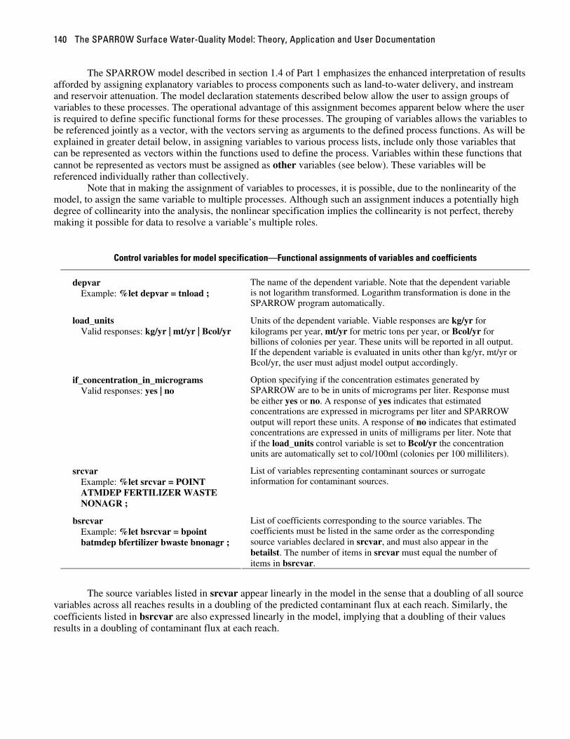
Control variables for model specification—Functional assignments of variables and coefficients
depvar Example: %let depvar = tnload ;
The name of the dependent variable. Note that the dependent variable is not logarithm transformed. Logarithm transformation is done in the SPARROW program automatically.
load_units Valid responses: kg/yr | mt/yr | Bcol/yr
Units of the dependent variable. Viable responses are kg/yr for kilograms per year, mt/yr for metric tons per year, or Bcol/yr for billions of colonies per year. These units will be reported in all output. If the dependent variable is evaluated in units other than kg/yr, mt/yr or Bcol/yr, the user must adjust model output accordingly.
if_concentration_in_micrograms Valid responses: yes | no
Option specifying if the concentration estimates generated by SPARROW are to be in units of micrograms per liter. Response must be either yes or no. A response of yes indicates that estimated concentrations are expressed in micrograms per liter and SPARROW output will report these units. A response of no indicates that estimated concentrations are expressed in units of milligrams per liter. Note that if the load_units control variable is set to Bcol/yr the concentration units are automatically set to col/100ml (colonies per 100 milliliters).
srcvar Example: %let srcvar = POINT ATMDEP FERTILIZER WASTE NONAGR ;
List of variables representing contaminant sources or surrogate information for contaminant sources.
bsrcvar Example: %let bsrcvar = bpoint batmdep bfertilizer bwaste bnonagr ;
List of coefficients corresponding to the source variables. The coefficients must be listed in the same order as the corresponding source variables declared in srcvar, and must also appear in the betailst. The number of items in srcvar must equal the number of items in bsrcvar.
The source variables listed in srcvar appear linearly in the model in the sense that a doubling of all source
variables across all reaches results in a doubling of the predicted contaminant flux at each reach. Similarly, the coefficients listed in bsrcvar are also expressed linearly in the model, implying that a doubling of their values results in a doubling of contaminant flux at each reach.
Part 2: SPARROW User’s Guide 141
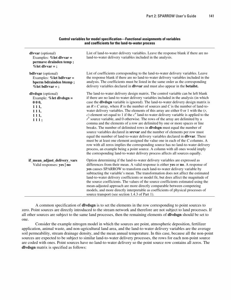
Control variables for model specification—Functional assignments of variables and coefficients for the land-to-water process
dlvvar (optional) Examples: %let dlvvar = permave drainden temp ; %let dlvvar = ;
List of land-to-water delivery variables. Leave the response blank if there are no land-to-water delivery variables included in the analysis.
bdlvvar (optional) Examples: %let bdlvvar = bperm bdrainden btemp ; %let bdlvvar = ;
List of coefficients corresponding to the land-to-water delivery variables. Leave the response blank if there are no land-to-water delivery variables included in the analysis. The coefficients must be listed in the same order as the corresponding delivery variables declared in dlvvar and must also appear in the betailst.
dlvdsgn (optional) Example: %let dlvdsgn = 0 0 0, 1 1 1, 1 1 1, 1 1 1, 1 1 1 ;
The land-to-water delivery design matrix. The control variable can be left blank if there are no land-to-water delivery variables included in the analysis (in which case the dlvdsgn variable is ignored). The land-to-water delivery design matrix is an R×C array, where R is the number of sources and C is the number of land-to-water delivery variables. The elements of this array are either 0 or 1 with the (r, c) element set equal to 1 if the cth land-to-water delivery variable is applied to the rth source variable, and 0 otherwise. The rows of the array are delimited by a comma and the elements of a row are delimited by one or more spaces or line breaks. The number of delimited rows in dlvdsgn must equal the number of source variables declared in srcvar and the number of elements per row must equal the number of land-to-water delivery variables declared in dlvvar. There must be at least one element assigned the value one in each of the C columns. A row with all zeros implies the corresponding source has no land-to-water delivery process, an example being a point source. A column with all ones would imply the corresponding land-to-water delivery process affects all sources equally.
if_mean_adjust_delivery_vars Valid responses: yes | no
Option determining if the land-to-water delivery variables are expressed as differences from their mean. A valid response is either yes or no. A response of yes causes SPARROW to transform each land-to-water delivery variable by subtracting the variable’s mean. The transformation does not affect the estimated land-to-water delivery coefficients or model fit, but does affect the magnitude of the source coefficients. The values of the source coefficients estimated using the mean-adjusted approach are more directly comparable between competeing models, and more directly interpretable as coefficients of physical processes of source transport (see section 1.4.3 of Part 1).
A common specification of dlvdsgn is to set the elements in the row corresponding to point sources to zero. Point sources are directly introduced to the stream network and therefore are not subject to land processes. If all other sources are subject to the same land processes, then the remaining elements of dlvdsgn should be set to one.
Consider the example nitrogen model in which the sources are point, atmospheric deposition, fertilizer application, animal waste, and non-agricultural land area, and the land-to-water delivery variables are the average soil permeability, stream drainage density, and the mean annual temperature. In this case, because all the non-point sources are expected to be subject to similar land-to-water delivery processes, the rows for each non-point source are coded with ones. Point sources have no land-to-water delivery so the point source row contains all zeros. The dlvdsgn matrix is specified as follows:
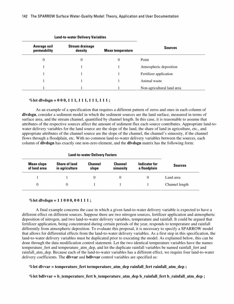
The SPARROW Surface Water-Quality Model: Theory, Application and User Documentation 142
Land-to-water Delivery Variables
Average soil permeability
Stream drainage density Mean temperature
Sources
0 0 0 Point
1 1 1 Atmospheric deposition
1 1 1 Fertilizer application
1 1 1 Animal waste
1 1 1 Non-agricultural land area
%let dlvdsgn = 0 0 0, 1 1 1, 1 1 1, 1 1 1, 1 1 1 ;
As an example of a specification that requires a different pattern of zeros and ones in each column of
dlvdsgn, consider a sediment model in which the sediment sources are the land surface, measured in terms of surface area, and the stream channel, quantified by channel length. In this case, it is reasonable to assume that attributes of the respective sources affect the amount of sediment flux each source contributes. Appropriate land-to-water delivery variables for the land source are the slope of the land, the share of land in agriculture, etc., and appropriate attributes of the channel source are the slope of the channel, the channel’s sinuosity, if the channel flows through a floodplain, etc. With no common land-to-water delivery variables between the sources, each column of dlvdsgn has exactly one non-zero element, and the dlvdsgn matrix has the following form:
Land-to-water Delivery Factors
Mean slope of land area
Share of land in agriculture
Channel slope
Channel sinuosity
Indicator for a floodplain
Sources
1 1 0 0 0 Land area
0 0 1 1 1 Channel length
%let dlvdsgn = 1 1 0 0 0, 0 0 1 1 1 ;
A final example concerns the case in which a given land-to-water delivery variable is expected to have a
different effect on different sources. Suppose there are two nitrogen sources, fertilizer application and atmospheric deposition of nitrogen, and two land-to-water delivery variables, temperature and rainfall. It could be argued that fertilizer application, being concentrated during certain periods of the year, responds to temperature and rainfall differently from atmospheric deposition. To evaluate this proposal, it is necessary to specify a SPARROW model that allows for differential effects from the land-to-water delivery variables. As a first step in this specification, the land-to-water delivery variables must be duplicated prior to executing the model. As explained below, this can be done through the data modification control statement. Let the two identical temperature variables have the names temperature_fert and temperature_atm_dep, and let the duplicate rainfall variables be named rainfall_fert and rainfall_atm_dep. Because each of the land-to-water variables has a different effect, we require four land-to-water delivery coefficients. The dlvvar and bdlvvar control variables are specified as:
%let dlvvar = temperature_fert termperature_atm_dep rainfall_fert rainfall_atm_dep ;
%let bdlvvar = b_temperature_fert b_temperature_atm_dep b_rainfall_fert b_rainfall_atm_dep ;
Part 2: SPARROW User’s Guide 143
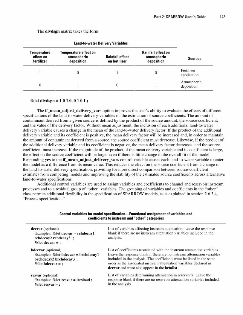
The dlvdsgn matrix takes the form:
Land-to-water Delivery Variables
Temperature effect on fertilizer
Temperature effect on atmospheric deposition
Rainfall effect on fertilizer
Rainfall effect on atmospheric deposition
Sources
1 0 1 0 Fertilizer application
0 1 0 1 Atmospheric deposition
%let dlvdsgn = 1 0 1 0, 0 1 0 1 ;
The if_mean_adjust_delivery_vars option improves the user’s ability to evaluate the effects of different
specifications of the land-to-water delivery variables on the estimation of source coefficients. The amount of contaminant derived from a given source is defined by the product of the source amount, the source coefficient, and the value of the delivery factor. Without mean adjustment, the inclusion of each additional land-to-water delivery variable causes a change in the mean of the land-to-water delivery factor. If the product of the additional delivery variable and its coefficient is positive, the mean delivery factor will be increased and, in order to maintain the amount of contaminant derived from a source, the source coefficient must decrease. Likewise, if the product of the additional delivery variable and its coefficient is negative, the mean delivery factor decreases, and the source coefficient must increase. If the magnitude of the product of the mean delivery variable and its coefficient is large, the effect on the source coefficient will be large, even if there is little change in the overall fit of the model. Responding yes to the if_mean_adjust_delivery_vars control variable causes each land-to-water variable to enter the model as a difference from its mean value. This reduces the effect on the source coefficient from a change in the land-to-water delivery specification, providing for more direct comparison between source-coefficient estimates from competing models and improving the stability of the estimated source coefficients across alternative land-to-water specifications.
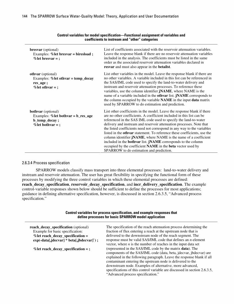
Additional control variables are used to assign variables and coefficients to channel and reservoir instream processes and to a residual group of “other” variables. The grouping of variables and coefficients in the “other” class permits additional flexibility in the specification of SPARROW models, as is explained in section 2.6.3.4, “Process specification.”
Control variables for model specification—Functional assignment of variables and coefficients to instream and “other” categories
decvar (optional) Examples: %let decvar = rchdecay1 rchdecay2 rchdecay3 ; %let decvar = ;
List of variables affecting instream attenuation. Leave the response blank if there are no instream attenuation variables included in the analysis.
bdecvar (optional) Examples: %let bdecvar = brchdecay1 brchdecay2 brchdecay3 ; %let bdecvar = ;
List of coefficients associated with the instream attenuation variables. Leave the response blank if there are no instream attenuation variables included in the analysis. The coefficients must be listed in the same order as the associated instream attenuation variables declared in decvar and must also appear in the betailst.
resvar (optional) Examples: %let resvar = iresload ; %let resvar = ;
List of variables determining attenuation in reservoirs. Leave the response blank if there are no reservoir attenuation variables included in the analysis.
The SPARROW Surface Water-Quality Model: Theory, Application and User Documentation 144
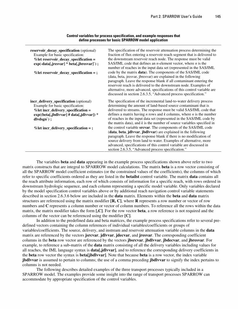
Control variables for model specification—Functional assignment of variables and coefficients to instream and “other” categories
bresvar (optional) Examples: %let bresvar = biresload ; %let bresvar = ;
List of coefficients associated with the reservoir attenuation variables. Leave the response blank if there are no reservoir attenuation variables included in the analysis. The coefficients must be listed in the same order as the associated reservoir attenuation variables declared in resvar and must also appear in the betailst.
othvar (optional) Examples: %let othvar = temp_decay res_age ; %let othvar = ;
List other variables in the model. Leave the response blank if there are no other variables. A variable included in this list can be referenced in the SAS/IML code used to specify the land-to-water delivery and instream and reservoir attenuation processes. To reference these variables, use the column identifier jNAME, where NAME is the name of a variable included in the othvar list. jNAME corresponds to the column occupied by the variable NAME in the input data matrix used by SPARROW to do estimation and prediction.
bothvar (optional) Examples: %let bothvar = b_res_age b_temp_decay ; %let bothvar = ;
List other coefficients in the model. Leave the response blank if there are no other coefficients. A coefficient included in this list can be referenced in the SAS IML code used to specify the land-to-water delivery and instream and reservoir attenuation processes. Note that the listed coefficients need not correspond in any way to the variables listed in the othvar statement. To reference these coefficients, use the column identifier jNAME, where NAME is the name of a coefficient included in the bothvar list. jNAME corresponds to the column occupied by the coefficient NAME in the beta vector used by SPARROW to do estimation and prediction.
2.6.3.4 Process specification
SPARROW models classify mass transport into three elemental processes: land-to-water delivery and instream and reservoir attenuation. The user has great flexibility in specifying the functional form of these processes by modifying the three control variables in which these elemental processes are defined: reach_decay_specification, reservoir_decay_specification, and incr_delivery_specification. The example control-variable responses shown below should be sufficient to define the processes for most applications; guidance in defining alternative specification, however, is discussed in section 2.6.3.5, “Advanced process specification.”
Control variables for process specification, and example responses that define processes for basic SPARROW model application
reach_decay_specification (optional) Example for basic specification: %let reach_decay_specification = exp(-data[,jdecvar] * beta[,jbdecvar]`) ; %let reach_decay_specification = ;
The specification of the reach attenuation process determining the fraction of flux entering a reach at the upstream node that is delivered to the downstream node of the reach segment. The response must be valid SAS/IML code that defines an n-element vector, where n is the number of reaches in the input data set (represented in the SAS/IML code by the matrix data). The components of the SAS/IML code (data, beta, jdecvar, jbdecvar) are explained in the following paragraph. Leave the response blank if all contaminant entering the upstream node is delivered to the downstream node. Examples of alternative, more advanced, specifications of this control variable are discussed in section 2.6.3.5, “Advanced process specification.”
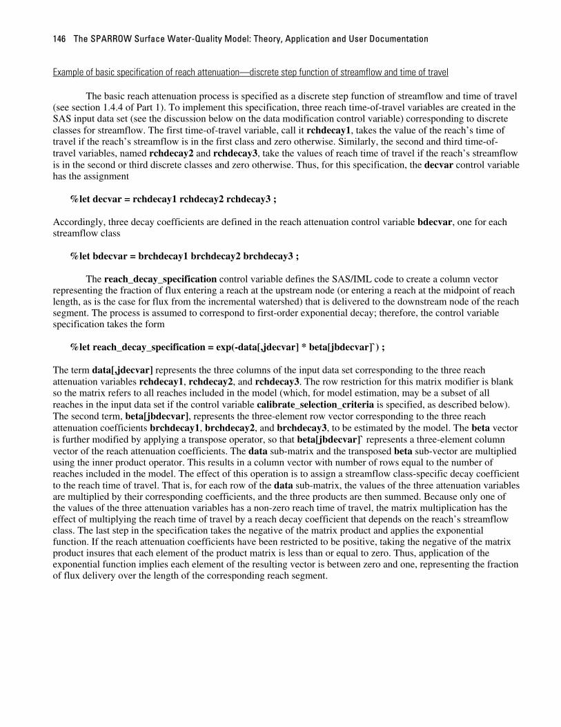
Part 2: SPARROW User’s Guide 145
Control variables for process specification, and example responses that define processes for basic SPARROW model application
reservoir_decay_specification (optional) Example for basic specification: %let reservoir_decay_specification = exp(-data[,jresvar] * beta[,jbresvar]`) ; %let reservoir_decay_specification = ;
The specification of the reservoir attenuation process determining the fraction of flux entering a reservoir reach segment that is delivered to the downstream reservoir reach node. The response must be valid SAS/IML code that defines an n-element vector, where n is the number of reaches in the input data set (represented in the SAS/IML code by the matrix data). The components of the SAS/IML code (data, beta, jresvar, jbresvar) are explained in the following paragraph. Leave the response blank if all contaminant entering the reservoir reach is delivered to the downstream node. Examples of alternative, more advanced, specifications of this control variable are discussed in section 2.6.3.5, “Advanced process specification.”
incr_delivery_specification (optional) Example for basic specification: %let incr_delivery_specification = exp((beta[,jbdlvvar] # data[,jdlvvar]) * dlvdsgn`) ; %let incr_delivery_specification = ;
The specification of the incremental land-to-water delivery process determining the amount of land-based source contaminant that is delivered to streams. The response must be valid SAS/IML code that defines a matrix having n rows and k columns, where n is the number of reaches in the input data set (represented in the SAS/IML code by the matrix data), and k is the number of source variables specified in the control variable srcvar. The components of the SAS/IML code (data, beta, jdlvvar, jbdlvvar) are explained in the following paragraph. Leave the response blank if there is no modification of source delivery from land to water. Examples of alternative, more advanced, specifications of this control variable are discussed in section 2.6.3.5, “Advanced process specification.”
The variables beta and data appearing in the example process specifications shown above refer to two
matrix constructs that are integral to SPARROW model calculations. The matrix beta is a row vector consisting of all the SPARROW model coefficient estimates (or the constrained values of the coefficients), the columns of which refer to specific coefficients ordered as they are listed in the betailst control variable. The matrix data contains all the reach attribute information, each row of which consists of information for a specific reach, with rows ordered in downstream hydrologic sequence, and each column representing a specific model variable. Only variables declared by the model specification control variables above or by additional reach navigation control variable statements described in section 2.6.3.6 below are included in the data matrix. Elements within the beta and data matrix structures are referenced using the matrix modifier [R, C], where R represents a row number or vector of row numbers and C represents a column number or vector of column numbers. To reference all the rows within the data matrix, the matrix modifier takes the form [,C]. For the row vector beta, a row reference is not required and the columns of the vector can be referenced using the modifier [C].
In addition to the predefined data and beta matrices, the example process specifications refer to several pre-defined vectors containing the column references of individual variables/coefficients or groups of variables/coefficients. The source, delivery, and instream and reservoir attenuation variable columns in the data matrix are referenced by the vectors jsrcvar, jdlvvar, jdecvar, and jresvar. The corresponding coefficient columns in the beta row vector are referenced by the vectors jbsrcvar, jbdlvvar, jbdecvar, and jbresvar. For example, to reference a sub-matrix of the data matrix consisting of all the delivery variables including values for all reaches, the IML language syntax is data[,jdlvvar], and to reference the corresponding delivery coefficients in the beta row vector the syntax is beta[jbdlvvar]. Note that because beta is a row vector, the index variable jbdlvvar is assumed to pertain to columns; the use of a comma preceding jbdlvvar to signify the index pertains to columns is not needed.
The following describes detailed examples of the three transport processes typically included in a SPARROW model. The examples provide some insight into the range of transport processes SPARROW can accommodate by appropriate specification of the control variables.
The SPARROW Surface Water-Quality Model: Theory, Application and User Documentation 146
Example of basic specification of reach attenuation—discrete step function of streamflow and time of travel
The basic reach attenuation process is specified as a discrete step function of streamflow and time of travel (see section 1.4.4 of Part 1). To implement this specification, three reach time-of-travel variables are created in the SAS input data set (see the discussion below on the data modification control variable) corresponding to discrete classes for streamflow. The first time-of-travel variable, call it rchdecay1, takes the value of the reach’s time of travel if the reach’s streamflow is in the first class and zero otherwise. Similarly, the second and third time-of-travel variables, named rchdecay2 and rchdecay3, take the values of reach time of travel if the reach’s streamflow is in the second or third discrete classes and zero otherwise. Thus, for this specification, the decvar control variable has the assignment
%let decvar = rchdecay1 rchdecay2 rchdecay3 ;
Accordingly, three decay coefficients are defined in the reach attenuation control variable bdecvar, one for each streamflow class
%let bdecvar = brchdecay1 brchdecay2 brchdecay3 ;
The reach_decay_specification control variable defines the SAS/IML code to create a column vector
representing the fraction of flux entering a reach at the upstream node (or entering a reach at the midpoint of reach length, as is the case for flux from the incremental watershed) that is delivered to the downstream node of the reach segment. The process is assumed to correspond to first-order exponential decay; therefore, the control variable specification takes the form
%let reach_decay_specification = exp(-data[,jdecvar] * beta[jbdecvar]`) ;
The term data[,jdecvar] represents the three columns of the input data set corresponding to the three reach attenuation variables rchdecay1, rchdecay2, and rchdecay3. The row restriction for this matrix modifier is blank so the matrix refers to all reaches included in the model (which, for model estimation, may be a subset of all reaches in the input data set if the control variable calibrate_selection_criteria is specified, as described below). The second term, beta[jbdecvar], represents the three-element row vector corresponding to the three reach attenuation coefficients brchdecay1, brchdecay2, and brchdecay3, to be estimated by the model. The beta vector is further modified by applying a transpose operator, so that beta[jbdecvar]` represents a three-element column vector of the reach attenuation coefficients. The data sub-matrix and the transposed beta sub-vector are multiplied using the inner product operator. This results in a column vector with number of rows equal to the number of reaches included in the model. The effect of this operation is to assign a streamflow class-specific decay coefficient to the reach time of travel. That is, for each row of the data sub-matrix, the values of the three attenuation variables are multiplied by their corresponding coefficients, and the three products are then summed. Because only one of the values of the three attenuation variables has a non-zero reach time of travel, the matrix multiplication has the effect of multiplying the reach time of travel by a reach decay coefficient that depends on the reach’s streamflow class. The last step in the specification takes the negative of the matrix product and applies the exponential function. If the reach attenuation coefficients have been restricted to be positive, taking the negative of the matrix product insures that each element of the product matrix is less than or equal to zero. Thus, application of the exponential function implies each element of the resulting vector is between zero and one, representing the fraction of flux delivery over the length of the corresponding reach segment.
Part 2: SPARROW User’s Guide 147
Example of basic specification of reservoir attenuation—discrete step function of reservoir flow rates
Although this specification of reservoir attenuation is not shown in the table above, it is described here because of its functional equivalence to the preceding example for basic specification of reach attenuation. In this example, reservoir attenuation is assumed to depend on reservoir time of travel and a discrete step function of reservoir flow rate. Reservoir time of travel is defined as the reservoir volume divided by the rate of outflow from the reservoir. Three variables for reservoir time of travel are created in the SAS input data set either by the user prior to model execution or through statements defined in the data modifications control variable (see section 2.6.3.8). As with the variable specification for the discrete function characterization of reach attenuation described above, the three variables correspond to the reservoir time of travel interacted with indicator variables identifying the throughput of the reach reservoir. Thus, the first reservoir decay variable, named resdecay1, takes the value of the reservoir time of travel if the reach reservoir throughput is in the first class, and zero otherwise. The other two reservoir decay variables, resdecay2 and resdecay3, are defined similarly for the second and third reservoir reach throughput classes.
The resvar control variable is specified to consist of the three reservoir decay variables
%let resvar = resdecay1 resdecay2 resdecay3 ; Accordingly, three reservoir attenuation coefficients are declared in the bresvar control variable
%let bresvar = bresdecay1 bresdecay2 bresdecay3 ;
The control-variable specification takes the form
%let reservoir_decay_specification = exp(-data[,jresvar] * beta[jbresvar]`) ; The specified reservoir attenuation process defines a column vector in which each element represents the fraction of flux entering the reach that is delivered to the outlet of the reach. For reaches that are not reservoirs, the three reservoir attenuation variables are equal to zero so that the corresponding element in the vector takes the value one. For reaches coded as reservoirs, one of the three reservoir attenuation variables is non-zero, taking the value of the reservoir time of travel. The effect of the matrix inner product operator is to multiply the reservoir time of travel by the reservoir attenuation coefficient (to be estimated by the model) corresponding to the reservoir’s throughput class.
Example of basic specification of reservoir attenuation—continuous function of settling rate represented by hydraulic load
The second example of a basic specification of reservoir attenuation uses the hydraulic load concept described in section 1.4.5 of Part 1. In this specification, the variable iresload (the inverse of the hydraulic load of the reservoir) is created in the SAS input data set and is derived from the ratio of reservoir surface area to reservoir outflow. The reservoir attenuation process depends on a single parameter (to be estimated by the model) that can be interpreted as the mean settling rate, in units of meters per year. The resvar and bresvar control variables take the form
%let resvar = iresload ; %let bresvar = bsettle_rate ;
The reservoir attenuation process assumes the rate of reservoir loss is equal to /(1 )x x+ , where x is the
settling rate coefficient divided by the hydraulic load; x therefore can be expressed in terms of the control variables for this example as the product of bresvar (the settling rate coefficient) and resvar (inverse hydraulic load). The fraction of flux delivered to the reservoir outlet therefore equals 1 - /(1 )x x+ , which simplifies to 1/(1 )x+ and is specified as
%let reservoir_decay_specification = 1 / (1 + data[,jresvar] * beta[,jbresvar]) ;
The SPARROW Surface Water-Quality Model: Theory, Application and User Documentation 148
The specification results in a column vector consisting of ones for reaches that are not reservoirs (iresload equals zero) and, if bsettle_rate is bounded below by zero, a value between zero and one for reaches classified as reservoirs. Note in this case it is not necessary to transpose the coefficient vector prior to matrix multiplication because beta[,jbresvar] is a scalar.
Example of basic specification of land-to-water delivery—product of delivery variables (exponentiated)
The basic specification of the land-to-water delivery process assumes the delivery factor is the product of delivery variables, each raised to an exponent that incorporates (through use of an on/off switch) considerations about specific source/delivery interactions. For source k, the functional form of this factor is
, ,
1
source delivery factor k mM
mm
k xγ
=
=∏
where mx represents delivery variable m, is its corresponding coefficient, and M is the number of delivery
variables. For this specification to be valid, it is necessary that each delivery variable take on only positive values. ,k mγ
The delivery factor given above is evaluated in SPARROW using an exponential function. Each of the delivery variables is first log transformed, using SAS assignment statements to redefine the delivery variables contained in the SAS input data set (see the discussion of the data_modifications control variable below). In this example, we assume there are three sources, point, fert and waste, corresponding to point sources, fertilizer application, and animal waste, and three delivery variables, perm, slope and temp, corresponding to soil permeability, mean incremental watershed slope, and mean temperature. The logarithm transformations of the delivery variables (either created by the user prior to model execution or through statements defined in the data_modifications control variable) are assigned the names lperm, lslope, and ltemp, and the associated coefficients are named blperm, blslope, and bltemp. The source variable and coefficient control variables are
%let srcvar = point fert waste ; %let bsrcvar = bpoint bfert bwaste ;
The delivery variable and coefficient control variables are
%let dlvvar = lperm lslope ltemp ; %let bdlvvar = blperm blslope bltemp ;
If the control variable if_mean_adjust_delivery_vars is assigned the value yes, each variable in dlvvar is further transformed (automatically) by expressing each variable as the difference from its mean.
The delivery design matrix (dlvdsgn) in this example has three rows (the number of source variables) and three columns (the number of delivery variables). The first row consists of zeros, representing the assumption that delivery variables do not affect the amount of point sources reaching the stream. The remaining sources are assumed to be identically influenced by each land-to-water delivery variable. Therefore, the dlvdsgn control variable is specified as
%let dlvdsgn = 0 0 0, 1 1 1, 1 1 1 ;
The land-to-water delivery process is specified using the incr_delivery_specification control variable as
%let incr_delivery_specification = exp((beta[,jbdlvvar] # data[,jdlvvar]) * dlvdsgn`) ;
The term data[,jdlvvar] corresponds to an n × 3 matrix, where n is the number of reaches in the analysis. The elements of data[,jdlvvar] are the logarithm transformed values of the delivery variables. The term beta[,jbdlvvar] represents a 3-element row vector of the corresponding land-to-water delivery coefficients
Part 2: SPARROW User’s Guide 149
(because beta is a row vector, the comma before jbdlvvar is not necessary). The data matrix is pre-multipled by the beta vector using the element-by-element multiplication operator (see section 2.6.3.5). The resulting n × 3 matrix is then matrix multiplied (again, see section 2.6.3.5) by the transposed 3 × 3 delivery design matrix to obtain an n × 3 matrix. The application of the exponential function results in an n × 3 matrix of land-to-water delivery factors having the functional form described above.
Modification of basic specification of land-to-water delivery
The specification in the previous example is quite flexible and can accommodate other possible functional forms. As discussed in section 1.4.3 of Part 1, an alternative approach is to specify the delivery process in such a way that the resulting estimates of delivery coefficients are all positive. This approach requires that delivery variables having a positive effect on delivery be transformed prior to model execution to their reciprocal form, and thereby requires that the user identify the direction of the effect of the delivery variable on transport prior to model execution. Subsequent to retransformation of the variables, the specification of the delivery process is similar to the basic example described above.
To illustrate this approach, suppose there are two delivery variables, soil permeability and stream drainage density. Soil permeability has a presumed inverse relation with delivery and drainage density has a presumed positive relation. Leaving the soil permeability variable untransformed and expressing the drainage density as its inverse (that is, 1/(drainage density)) for a specification should result in negative values for the estimated delivery coefficients (using the same delivery specification as the previous example). Let the name of the untransformed permeability variable be perm and let the name of the inverse drainage density variable be idrainden. The dlvvar and bdlvvar control variables are defined as
%let dlvvar = perm idrainden ; %let bdlvvar = bperm bidrainden ;
As above, let the sources be point, fert and waste. In this case, the delivery design matrix has three rows (corresponding to the three sources) and two columns (corresponding to the two delivery variables), taking the form
%let dlvdsgn = 0 0, 1 1, 1 1 ;
The land-to-water delivery specification is similar to the form in the previous example, except a negative sign is placed before the beta[,jbdlvvar] term
%let incr_delivery_specification = exp((-beta[,jbdlvvar] # data[,jdlvvar]) * dlvdsgn`) ;
The approach to land-to-water delivery specification just described is similar to that used in previous SPARROW applications (Smith and others, 1997, and Alexander and others, 2001). A model estimated using this specification is viable if the resulting coefficient estimates for bperm and bidrainden are both positive; the user may wish to impose this constraint by modifying the betailst specification for these coefficients.
Linking SPARROW to deterministic process models
The examples described above use an exclusively empirical approach to process specification: all process coefficients are estimated using the SPARROW modeling framework. It is also possible, however, to incorporate deterministic processes into the analysis. One approach is to define the deterministic process as a variable in the SAS input data set and then incorporate this variable into the SPARROW model with an estimated coefficient.
For example, it has been argued that the amount of contaminant originating on the land surface that is delivered to a stream depends on the flow pathway connecting the land to the stream. Non-dissolved contaminants are transported only by overland flow pathways, whereas dissolved contaminants are transported both overland and through the subsurface, with subsurface transport related inversely to length of subsurface pathways. The SPARROW model can be used to evaluate the empirical importance of the overland flow process by evaluating the statistical significance of estimates of overland flow derived from deterministic modeling.
The SPARROW Surface Water-Quality Model: Theory, Application and User Documentation 150
The deterministic model TOPMODEL has been used to make estimates of the fraction of generated streamflow that is overland flow (Dunne or Horton overland flow) as opposed to subsurface flow (Wolock, 1993). Output from TOPMODEL can be used to create an additional variable in the SAS input data file, call it lfrac_overland, representing the logarithm of the fraction of streamflow emanating from each incremental watershed that arises from overland processes. This variable, along with an associated coefficient, is then declared in the dlvvar and bdlvvar control variables. The land-to-water delivery specification is the same as in the first example. The deterministic process is empirically verified if the estimated value for the coefficient associated with lfrac_overland is statistically significant.
2.6.3.5 Advanced process specification
It is recommended that users who wish to modify the delivery specification control variables from the basic forms described above become familiar with basic commands from the SAS Interactive Matrix Language (SAS/IML), in which the SPARROW model algorithms are written. It is highly recommended that prior to model execution the user test modified process specification in an interactive PROC IML SAS session using a sample data matrix and coefficient vector. The basic operations and rules for working in SAS/IML are included here as a brief introduction and review.
Matrices can be defined by entering value elements into an array. To define an n × k matrix from individual elements, the elements are listed within braces, { }, in row major order using spaces to delineate columns and commas to delineate rows. For example, to create the 2 × 3 matrix
1 3 42 0 8⎡ ⎤⎢ ⎥⎢ ⎥⎣ ⎦
,
the SAS/IML statement is {1 3 4, 2 0 8}. The basic matrix operators useful in specifying the processes are:
Basic matrix operators used in SAS/IML
* Matrix multiplication (inner or dot product) between two matrices with conforming dimensions. Usage: A * B, where A is n × k and B is k × m (unless A or B are scalars).
# Element-by-element product of two matrices having the same dimensions. Usage: A # B, where A is n × k and B is n × k, unless A or B are vectors (see below).
Element-by-element division of two matrices having the same dimensions. Usage: A / B, where A is n × k and B is n × k (unless A or B are scalars).
/
Element-by-element addition of two matrices having the same dimensions. Usage: A + B, where A is n × k and B is n × k (unless A or B are scalars).
+
Element-by-element subtraction of two matrices having the same dimensions. Usage: A – B, where A is n × k and B is n × k (unless A or B are scalars).
-
## Element-by-element power operator of two matrices having the same dimensions. Usage: A ## B, where A is n × k and B is n × k (unless A or B are scalars), results in an n × k matrix in which each element is the corresponding element of A raised to the power given by the corresponding element of B.
Element-by-element maximum. Usage: A <> B, where A is n × k and B is n × k (unless A or B are scalars), results in an n × k matrix in which each element is the maximum of the corresponding elements of A and B.
<>
Element-by-element minimum. Usage: A >< B, where A is n × k and B is n × k (unless A or B are scalars), results in an n × k matrix in which each element is the minimum of the corresponding elements of A and B.
><
|| Horizontal concatenation of two matrices having conforming row dimensions. Usage: A || B, where A is n × k and B is n × m, results in an n × (k + m) matrix.
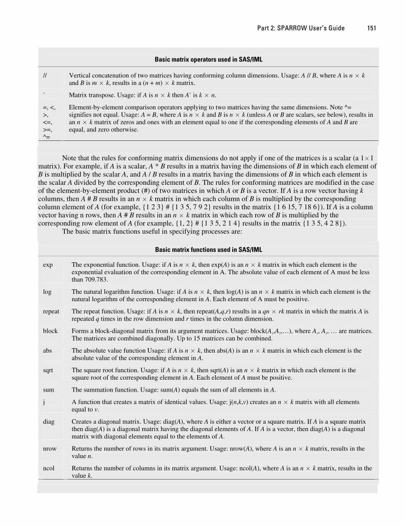
Part 2: SPARROW User’s Guide 151
Basic matrix operators used in SAS/IML
Vertical concatenation of two matrices having conforming column dimensions. Usage: A // B, where A is n × k and B is m × k, results in a (n + m) × k matrix.
//
Matrix transpose. Usage: if A is n × k then A` is k × n. `
=, <, >, <=, >=, ^=
Element-by-element comparison operators applying to two matrices having the same dimensions. Note ^= signifies not equal. Usage: A = B, where A is n × k and B is n × k (unless A or B are scalars, see below), results in an n × k matrix of zeros and ones with an element equal to one if the corresponding elements of A and B are equal, and zero otherwise.
Note that the rules for conforming matrix dimensions do not apply if one of the matrices is a scalar (a 1×1
matrix). For example, if A is a scalar, A * B results in a matrix having the dimensions of B in which each element of B is multiplied by the scalar A, and A / B results in a matrix having the dimensions of B in which each element is the scalar A divided by the corresponding element of B. The rules for conforming matrices are modified in the case of the element-by-element product (#) of two matrices in which A or B is a vector. If A is a row vector having k columns, then A # B results in an n × k matrix in which each column of B is multiplied by the corresponding column element of A (for example, {1 2 3} # {1 3 5, 7 9 2} results in the matrix {1 6 15, 7 18 6}). If A is a column vector having n rows, then A # B results in an n × k matrix in which each row of B is multiplied by the corresponding row element of A (for example, {1, 2} # {1 3 5, 2 1 4} results in the matrix {1 3 5, 4 2 8}).
The basic matrix functions useful in specifying processes are:
Basic matrix functions used in SAS/IML
The exponential function. Usage: if A is n × k, then exp(A) is an n × k matrix in which each element is the exponential evaluation of the corresponding element in A. The absolute value of each element of A must be less than 709.783.
exp
The natural logarithm function. Usage: if A is n × k, then log(A) is an n × k matrix in which each element is the natural logarithm of the corresponding element in A. Each element of A must be positive.
log
The repeat function. Usage: if A is n × k, then repeat(A,q,r) results in a qn × rk matrix in which the matrix A is repeated q times in the row dimension and r times in the column dimension.
repeat
block Forms a block-diagonal matrix from its argument matrices. Usage: block(A1,A2,…), where A1, A2, … are matrices. The matrices are combined diagonally. Up to 15 matrices can be combined.
The absolute value function Usage: if A is n × k, then abs(A) is an n × k matrix in which each element is the absolute value of the corresponding element in A.
abs
The square root function. Usage: if A is n × k, then sqrt(A) is an n × k matrix in which each element is the square root of the corresponding element in A. Each element of A must be positive.
sqrt
sum The summation function. Usage: sum(A) equals the sum of all elements in A.
A function that creates a matrix of identical values. Usage: j(n,k,v) creates an n × k matrix with all elements equal to v.
j
diag Creates a diagonal matrix. Usage: diag(A), where A is either a vector or a square matrix. If A is a square matrix then diag(A) is a diagonal matrix having the diagonal elements of A. If A is a vector, then diag(A) is a diagonal matrix with diagonal elements equal to the elements of A.
Returns the number of rows in its matrix argument. Usage: nrow(A), where A is an n × k matrix, results in the value n.
nrow
Returns the number of columns in its matrix argument. Usage: ncol(A), where A is an n × k matrix, results in the value k.
ncol

The SPARROW Surface Water-Quality Model: Theory, Application and User Documentation 152
Example of advanced specification of reach attenuation—continuous function (with upper and lower bounds) of stream depth and time of travel
This example describes a case in which reach attenuation is a continuous function of stream depth and time of travel. The practical motivation for this specification is discussed in section 1.4.4 of Part 1 and a depiction of the process is given in figure 1.17. The process relates the rate of attenuation to stream depth and assumes a cut-off in the tails of the relation. The process described below specifies the cut-off depths as coefficients to be estimated in the model—although practical application of this specification shows that it may be difficult to obtain valid estimates of these cut-off values. Additionally, the process includes an additive coefficient and an additional coefficient multiplied by stream depth. The functional form of the relation is
10 l
low
10 low
10 h
hi
, if
decay rate , if
, if
D DD
D D DD
D DD
δδ
δδ
δδ
⎧⎪⎪ + ≤⎪⎪⎪⎪⎪⎪⎪= + < ≤⎨⎪⎪⎪⎪⎪ + >⎪⎪⎪⎪⎩
ow
hi
i
,
where D is stream depth, Dlow and Dhi are lower and upper cut-offs for stream depth (to be estimated), and and 0δ
1δ are the additive and multiplicative decay coefficients, respectively. The fraction of flux entering the reach from
upstream that is delivered to the downstream node is determined by applying the exponential function to the negative product of the decay rate and the value of the reach time of travel.
The reach attenuation process based on stream depth is defined in SPARROW as follows. First, the stream depth variable must be created in the SAS input data set. Stream depth can be created from streamflow using a SAS assignment command in the data modification specification (described in section 2.6.3.8)
depth = .2612 * meanq ** .3966 ;
where meanq is streamflow in meters3 second-1. In this example, the reach attenuation process is specified using the othvar and bothvar control variables
%let othvar = rchtot depth ;
%let bothvar = brchdecay0 brchdecay1 bdepth_lo bdepth_dif ;
where brchdecay0 and brchdecay1 correspond to and , bdepth_lo corresponds to D0δ 1δ low, and the sum of
bdepth_lo and bdepth_dif corresponds to Dhi. The coefficients bdepth_lo and bdepth_dif are constrained to be positive in the betailst control variable, insuring that Dlow is positive and Dhi is greater than Dlow.
The attenuation function is specified using the reach_decay_specification control variable
%let reach_decay_specification = exp(-data[,jrchtot] # (beta[,jbrchdecay0] +
beta[,jbrchdecay1] / ((beta[,jbdepth_hi] + beta[,jbdepth_lo]) ><
(beta[,jbdepth_lo] <> data[,jdepth])))) ;
As with the first example, the reach delivery function is an exponential function of the negative of reach time of travel. The term data[,jrchtot] is a column vector representing the time of travel values for each reach. The elements of this vector are multiplied by the additive decay coefficient, given by the scalar beta[,jbrchdecay0], and a second term representing the effect of stream depth on reach attenuation. The denominator of the second term

Part 2: SPARROW User’s Guide 153
is evaluated using the element-by-element minimum and maximum operator: the first operation (<>) compares stream depth to the coefficient bdepth_lo (which bounds the lower tail of stream depth) and returns the larger of the two; the second operator (><) compares stream depth to the sum of bdepth_lo and bdepth_dif (this sum bounds the upper tail of depth) and returns the smaller of the two. The denominator is therefore evaluated either as equal to stream depth or, if the stream depth lies outside the upper or lower bound, as equal to the respective bound.
Example of advanced specification of reservoir attenuation—continuous function of settling rate represented as function of hydraulic load and temperature
In this example, the process specified in a previous reservoir attenuation example is modified by introducing temperature as an additional variable affecting reservoir attenuation. This modification is based on the Arrhenius equation having the general form
20TTk kb −= ,
where kT is a temperature-dependent reaction rate, k is the standard reaction rate—assumed here to be determined by the reservoir hydraulic load, b is an estimated coefficient, and T is temperature in degrees Celsius.
In addition to the iresload variable (inverse hydraulic load, see previous example) the SAS input file is assumed to include a re-centered temperature variable, named rwtempdif, given by
rwtempdif = wtemp - 20.0 ;
where wtemp is water temperature in degrees Celsius. As in the previous example, the inverse hydraulic load and the settling rate are declared as a reservoir
decay variable and coefficient. The temperature variable and coefficient cannot be declared similarly (that is, as a second reservoir decay variable and coefficient), however, because they enter the process specification non-symmetrically (with respect to the hydraulic load and settling rate). Instead, the temperature variable and coefficient must be declared in the model using the othvar and bothvar control variables. The reservoir and other variable and coefficient declarations are therefore
%let resvar = iresload ;
%let bresvar = bsettle_rate ;
%let othvar = rwtempdif ;
%let bothvar = brwtempdif ;
The reservoir attenuation process is redefined so that the Arrhenius function is integrated with the hydraulic load term (see section 1.4.5 of Part 1)
%let reservoir_decay_specification = 1 / (1 + (data[,jresvar] * beta[,jbresvar]) #
beta[,jbrwtempdif] ## data[,jrwtempdif] ) ;
Note that both the variable rwtempdif and the coefficient brwtempdif must be referenced explicitly in the control variable specification (rather than by their namelist variables othvar and bothvar); this rule applies for any variable-coefficient pair declared in the othvar and bothvar specifications. The Arrhenius function is evaluated by raising the scalar beta[,jbrwtempdif] to a power defined by the column vector data[,jrwtempdif]. This operation results in a column vector that is then integrated with the hydraulic load term from the previous specification using element-by-element multiplication.
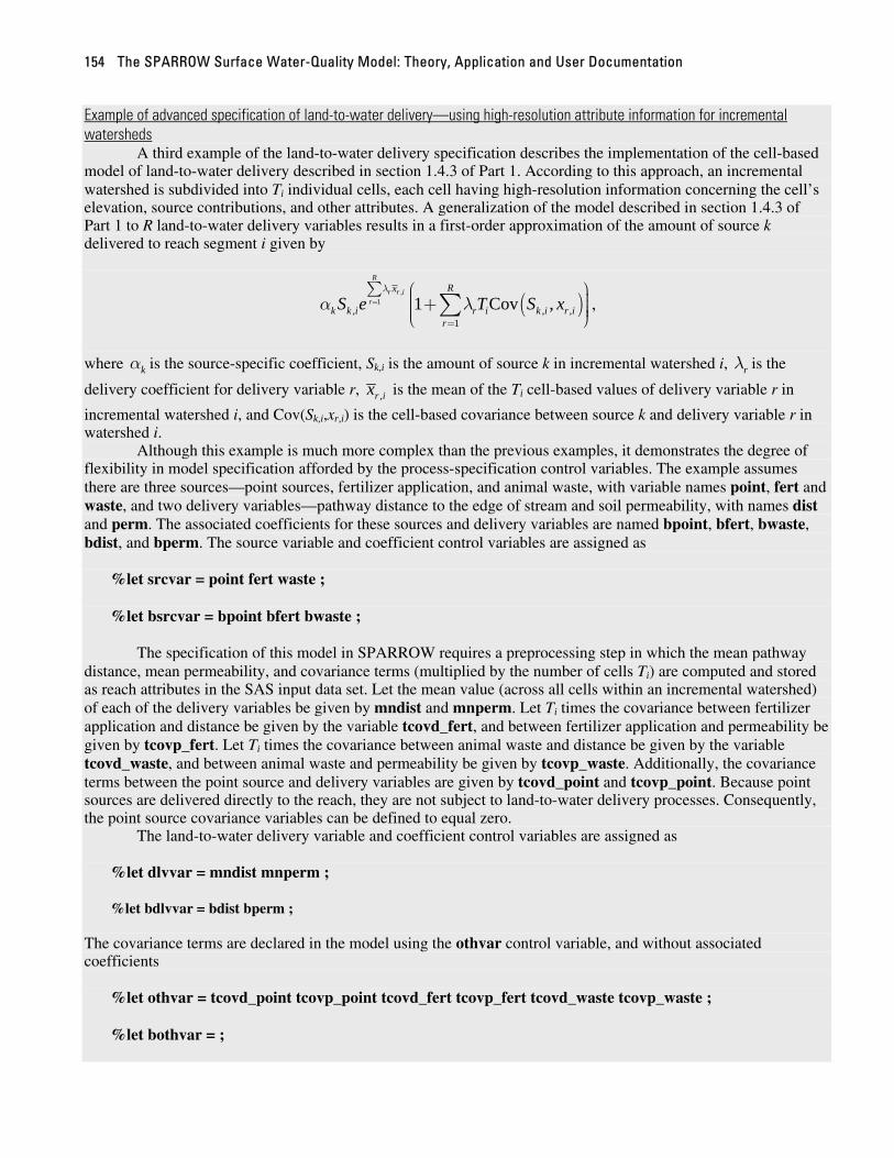
The SPARROW Surface Water-Quality Model: Theory, Application and User Documentation 154
Example of advanced specification of land-to-water delivery—using high-resolution attribute information for incremental watersheds
A third example of the land-to-water delivery specification describes the implementation of the cell-based model of land-to-water delivery described in section 1.4.3 of Part 1. According to this approach, an incremental watershed is subdivided into Ti individual cells, each cell having high-resolution information concerning the cell’s elevation, source contributions, and other attributes. A generalization of the model described in section 1.4.3 of Part 1 to R land-to-water delivery variables results in a first-order approximation of the amount of source k delivered to reach segment i given by
( ),
1, ,
1
1 Cov ,
R
r r ir
Rx
k k i r i k i r ir
S e T S xλ
α λ=
=
∑ ⎛ ⎞⎟⎜ + ⎟⎜ ⎟⎜ ⎟⎝ ⎠∑ , ,
where is the source-specific coefficient, Skα k,i is the amount of source k in incremental watershed i, is the rλdelivery coefficient for delivery variable r, ,r ix is the mean of the Ti cell-based values of delivery variable r in
incremental watershed i, and Cov(Sk,i,xr,i) is the cell-based covariance between source k and delivery variable r in watershed i.
Although this example is much more complex than the previous examples, it demonstrates the degree of flexibility in model specification afforded by the process-specification control variables. The example assumes there are three sources—point sources, fertilizer application, and animal waste, with variable names point, fert and waste, and two delivery variables—pathway distance to the edge of stream and soil permeability, with names dist and perm. The associated coefficients for these sources and delivery variables are named bpoint, bfert, bwaste, bdist, and bperm. The source variable and coefficient control variables are assigned as
%let srcvar = point fert waste ;
%let bsrcvar = bpoint bfert bwaste ;
The specification of this model in SPARROW requires a preprocessing step in which the mean pathway distance, mean permeability, and covariance terms (multiplied by the number of cells Ti) are computed and stored as reach attributes in the SAS input data set. Let the mean value (across all cells within an incremental watershed) of each of the delivery variables be given by mndist and mnperm. Let Ti times the covariance between fertilizer application and distance be given by the variable tcovd_fert, and between fertilizer application and permeability be given by tcovp_fert. Let Ti times the covariance between animal waste and distance be given by the variable tcovd_waste, and between animal waste and permeability be given by tcovp_waste. Additionally, the covariance terms between the point source and delivery variables are given by tcovd_point and tcovp_point. Because point sources are delivered directly to the reach, they are not subject to land-to-water delivery processes. Consequently, the point source covariance variables can be defined to equal zero.
The land-to-water delivery variable and coefficient control variables are assigned as
%let dlvvar = mndist mnperm ;
%let bdlvvar = bdist bperm ;
The covariance terms are declared in the model using the othvar control variable, and without associated coefficients
%let othvar = tcovd_point tcovp_point tcovd_fert tcovp_fert tcovd_waste tcovp_waste ;
%let bothvar = ;

Part 2: SPARROW User’s Guide 155
The delivery factors are assumed to apply equally to fertilizer and animal waste. The delivery design matrix has three rows and two columns and is defined as
%let dlvdsgn = 0 0, 1 1, 1 1 ;
The land-to-water delivery specification is defined as
%let incr_delivery_specification =
exp((data[,jdlvvar] # beta[,jbdlvvar]) * dlvdsgn`) #
(1 + ((data[,jtcovd_point || jtcovp_point || jtcovd_fert || jtcovp_fert ||
jtcovd_waste || jtcovp_waste] # repeat(beta[,jbdlvvar],1,3)) *
block(dlvdsgn[1,],dlvdsgn[2,],dlvdsgn[3,])`) ;
The exponential term in this specification is identical to the delivery specifications given in previous examples. This term represents a n × k matrix, where n is the number of reaches in the analysis and k is the number of sources. The term data[,jtcovd_point || jtcovp_point || jtcovd_fert || jtcovp_fert || jtcovd_waste || jtcovp_waste] represents a six-column matrix corresponding to the covariances between the three sources—point, fertilizer, and waste—and the two delivery variables—distance and permeability. This matrix is element-by-element multiplied by a 6-element row vector consisting of three repeated values of the two-element delivery coefficients row vector (repeat(beta[,jbdlvvar],1,3)). The resulting matrix consists of six columns. This matrix is post multiplied by a block-modified delivery design matrix, the result being a matrix having three columns, each column corresponding to a source in the model. The value one is added to each element of this matrix and the result is element-by-element multiplied with the three-column matrix of exponential terms.
2.6.3.6 Additional variable definitions
The control variables described below represent variables required by SPARROW to navigate the reach network, compute alternative prediction output (e.g., yield and concentration), identify water-quality monitoring stations and their locations, assign weights in the least squares algorithm, provide ancillary information in the output, and identify target locations for estimating delivery ratios. As with the name-list variables defined above, each variable identified in the response to these control variables must be included in the SAS input data or created from existing variables in the SAS input data using the data modifications specification described below. Variable names given in the response can be up to 32 characters and cannot include any special characters except the underscore. In cases where a list is requested, the listed items must be separated by one or more spaces or line breaks.
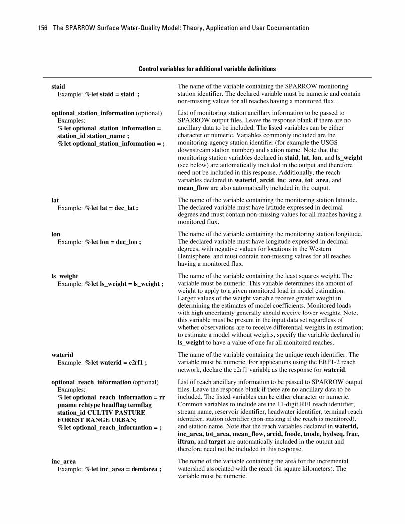
The SPARROW Surface Water-Quality Model: Theory, Application and User Documentation 156
Control variables for additional variable definitions
staid Example: %let staid = staid ;
The name of the variable containing the SPARROW monitoring station identifier. The declared variable must be numeric and contain non-missing values for all reaches having a monitored flux.
optional_station_information (optional) Examples: %let optional_station_information = station_id station_name ; %let optional_station_information = ;
List of monitoring station ancillary information to be passed to SPARROW output files. Leave the response blank if there are no ancillary data to be included. The listed variables can be either character or numeric. Variables commonly included are the monitoring-agency station identifier (for example the USGS downstream station number) and station name. Note that the monitoring station variables declared in staid, lat, lon, and ls_weight (see below) are automatically included in the output and therefore need not be included in this response. Additionally, the reach variables declared in waterid, arcid, inc_area, tot_area, and mean_flow are also automatically included in the output.
lat Example: %let lat = dec_lat ;
The name of the variable containing the monitoring station latitude. The declared variable must have latitude expressed in decimal degrees and must contain non-missing values for all reaches having a monitored flux.
lon Example: %let lon = dec_lon ;
The name of the variable containing the monitoring station longitude. The declared variable must have longitude expressed in decimal degrees, with negative values for locations in the Western Hemisphere, and must contain non-missing values for all reaches having a monitored flux.
ls_weight Example: %let ls_weight = ls_weight ;
The name of the variable containing the least squares weight. The variable must be numeric. This variable determines the amount of weight to apply to a given monitored load in model estimation. Larger values of the weight variable receive greater weight in determining the estimates of model coefficients. Monitored loads with high uncertainty generally should receive lower weights. Note, this variable must be present in the input data set regardless of whether observations are to receive differential weights in estimation; to estimate a model without weights, specify the variable declared in ls_weight to have a value of one for all monitored reaches.
waterid Example: %let waterid = e2rf1 ;
The name of the variable containing the unique reach identifier. The variable must be numeric. For applications using the ERF1-2 reach network, declare the e2rf1 variable as the response for waterid.
optional_reach_information (optional) Examples: %let optional_reach_information = rr pname rchtype headflag termflag station_id CULTIV PASTURE FOREST RANGE URBAN; %let optional_reach_information = ;
List of reach ancillary information to be passed to SPARROW output files. Leave the response blank if there are no ancillary data to be included. The listed variables can be either character or numeric. Common variables to include are the 11-digit RF1 reach identifier, stream name, reservoir identifier, headwater identifier, terminal reach identifier, station identifier (non-missing if the reach is monitored), and station name. Note that the reach variables declared in waterid, inc_area, tot_area, mean_flow, arcid, fnode, tnode, hydseq, frac, iftran, and target are automatically included in the output and therefore need not be included in this response.
inc_area Example: %let inc_area = demiarea ;
The name of the variable containing the area for the incremental watershed associated with the reach (in square kilometers). The variable must be numeric.
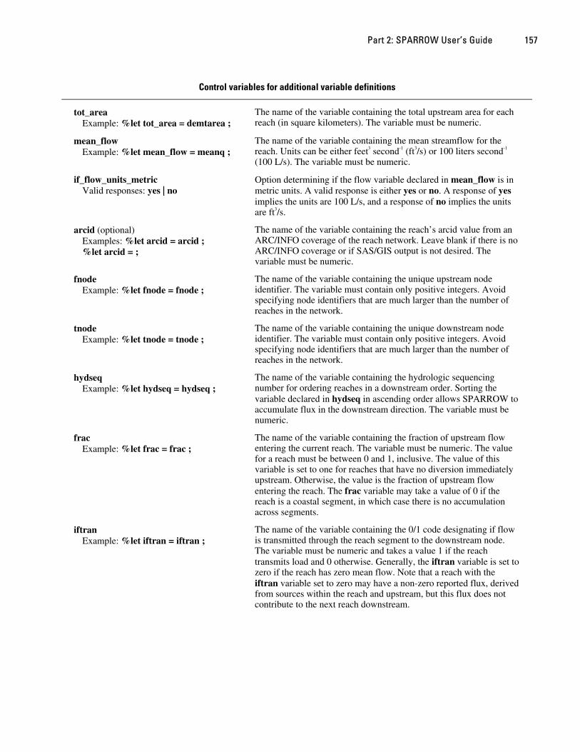
Part 2: SPARROW User’s Guide 157
Control variables for additional variable definitions
tot_area Example: %let tot_area = demtarea ;
The name of the variable containing the total upstream area for each reach (in square kilometers). The variable must be numeric.
mean_flow Example: %let mean_flow = meanq ;
The name of the variable containing the mean streamflow for the reach. Units can be either feet3 second-1 (ft3/s) or 100 liters second-1 (100 L/s). The variable must be numeric.
if_flow_units_metric Valid responses: yes | no
Option determining if the flow variable declared in mean_flow is in metric units. A valid response is either yes or no. A response of yes implies the units are 100 L/s, and a response of no implies the units are ft3/s.
arcid (optional) Examples: %let arcid = arcid ; %let arcid = ;
The name of the variable containing the reach’s arcid value from an ARC/INFO coverage of the reach network. Leave blank if there is no ARC/INFO coverage or if SAS/GIS output is not desired. The variable must be numeric.
fnode Example: %let fnode = fnode ;
The name of the variable containing the unique upstream node identifier. The variable must contain only positive integers. Avoid specifying node identifiers that are much larger than the number of reaches in the network.
tnode Example: %let tnode = tnode ;
The name of the variable containing the unique downstream node identifier. The variable must contain only positive integers. Avoid specifying node identifiers that are much larger than the number of reaches in the network.
hydseq Example: %let hydseq = hydseq ;
The name of the variable containing the hydrologic sequencing number for ordering reaches in a downstream order. Sorting the variable declared in hydseq in ascending order allows SPARROW to accumulate flux in the downstream direction. The variable must be numeric.
frac Example: %let frac = frac ;
The name of the variable containing the fraction of upstream flow entering the current reach. The variable must be numeric. The value for a reach must be between 0 and 1, inclusive. The value of this variable is set to one for reaches that have no diversion immediately upstream. Otherwise, the value is the fraction of upstream flow entering the reach. The frac variable may take a value of 0 if the reach is a coastal segment, in which case there is no accumulation across segments.
iftran Example: %let iftran = iftran ;
The name of the variable containing the 0/1 code designating if flow is transmitted through the reach segment to the downstream node. The variable must be numeric and takes a value 1 if the reach transmits load and 0 otherwise. Generally, the iftran variable is set to zero if the reach has zero mean flow. Note that a reach with the iftran variable set to zero may have a non-zero reported flux, derived from sources within the reach and upstream, but this flux does not contribute to the next reach downstream.
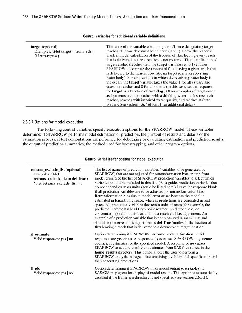
The SPARROW Surface Water-Quality Model: Theory, Application and User Documentation 158
Control variables for additional variable definitions
target (optional) Examples: %let target = term_rch ; %let target = ;
The name of the variable containing the 0/1 code designating target reaches. The variable must be numeric (0 or 1). Leave the response blank if model calculation of the fraction of flux leaving every reach that is delivered to target reaches is not required. The identification of target reaches (reaches with the target variable set to 1) enables SPARROW to compute the amount of flux leaving a given reach that is delivered to the nearest downstream target reach (or receiving water body). For applications in which the receiving water body is the ocean, the target variable takes the value 1 for all estuary and coastline reaches and 0 for all others. (In this case, set the response for target as a function of termflag.) Other examples of target-reach assignments include reaches with a drinking-water intake, reservoir reaches, reaches with impaired water quality, and reaches at State borders. See section 1.6.7 of Part 1 for additional details.
2.6.3.7 Options for model execution
The following control variables specify execution options for the SPARROW model. These variables determine: if SPARROW performs model estimation or prediction, the printout of results and details of the estimation process, if test computations are peformed for debugging or evaluating estimation and prediction results, the output of prediction summaries, the method used for bootstrapping, and other program options.
Control variables for options for model execution
retrans_exclude_list (optional) Examples: %let retrans_exclude_list = del_frac ; %let retrans_exclude_list = ;
The list of names of prediction variables (variables to be generated by SPARROW) that are not adjusted for retransformation bias arising from model error. See the list of SPARROW prediction variables to select which variables should be included in this list. (As a guide, prediction variables that do not depend on mass units should be listed here.) Leave the response blank if all prediction variables are to be adjusted for retransformation bias. Retransformation bias due to model error arises because the model is estimated in logarithmic space, whereas predictions are generated in real space. All prediction variables that retain units of mass (for example, the predicted incremental load from point sources, predicted yield, or concentration) exhibit this bias and must receive a bias adjustment. An example of a prediction variable that is not measured in mass units and should not receive a bias adjustment is del_frac (unitless) -the fraction of flux leaving a reach that is delivered to a downstream target location.
if_estimate Valid responses: yes | no
Option determining if SPARROW performs model estimation. Valid responses are yes or no. A response of yes causes SPARROW to generate coefficient estimates for the specified model. A response of no causes SPARROW to acquire coefficient estimates from SAS files stored in the home_results directory. This option allows the user to perform a SPARROW analysis in stages; first obtaining a valid model specification and then generating predictions.
if_gis Valid responses: yes | no
Option determining if SPARROW links model output (data tables) to SAS/GIS maplayers for display of model results. This option is automatically disabled if the home_gis directory is not specified (see section 2.6.3.1).

Part 2: SPARROW User’s Guide 159
Control variables for options for model execution
calibrate_selection_criteria (optional)
Examples: %let calibrate_selection_criteria = &WATERID > 0 & &waterid < 80000 & &hydseq > 0 ; %let calibrate_selection_criteria = ;
The SAS code used to select reach observations from the input data set (the file declared in the control variable indata) that are used to estimate the SPARROW model. Leave the response blank if all reaches are to be included in model estimation. The set of reaches used in model estimation can be smaller than the set used in prediction; for example, reaches downstream from all monitoring stations can be excluded from the estimation set because they have no effect on estimation results. Excluding these reaches from estimation speeds up the estimation algorithm. In the example shown at left, reaches known to be located downstream from all monitoring stations are identified by values of the waterid variable and excluded.
NLP_printing_option Valid responses: any integer between 0 and 5
The nonlinear optimization procedure printing option. A valid response is an integer between 0 and 5. A higher integer causes model results from a greater number of the optimization steps to be printed to the SAS Output window. The options are: 0 No optimization results are printed to the Output window. 1 The summaries for optimization start and termination, as well as the iteration history, are printed. 2 The initial and final parameter estimates are also printed. 3 The values of the termination criteria and other control parameters are also printed. 4 The parameter vector, x, is also printed after each iteration. 5 The gradient vector, g, is also printed after each iteration. For a bootstrap analysis that reestimates the model for each bootstrap iteration it is recommended that the NLP printing option be set to 0 to avoid excessive output.
if_test_calibrate Valid responses: yes | no
Option determining if SPARROW estimates the model in test mode. Valid responses are yes or no. Run SPARROW in this test mode (respond yes) after a SPARROW execution fails upon evaluation of coefficients at initial values (no output after listing initial values). In this test mode, SPARROW lists waterid and relevant stream attenuation and land-to-water delivery variables for observations that, when evaluated at initial parameter values, cause an error due to applying an exponential function that results in a numerical overflow condition. (Large values in the stream attenuation and land-to-water delivery variables typically underlie these errors.) SPARROW in test mode also checks for negative reach values of the stream and reservoir attenuation factors, the incremental flux, and for non-positive values of the accumulated flux at monitoring stations (evaluated at the initial coefficient values). In test mode, the if_accumulate_with_dll option (see below) is automatically set to no to obtain more informative error flagging. See section 2.9.2.2, “Estimation errors caused by numerical overflow,” for additional information.
if_accumulate_with_dll Valid responses: yes | no
Option determining if SPARROW estimates the model using the dynamically linked library (DLL) code in the file “sparrow.dll” to accumulate flux across the reach network. Valid responses are yes or no. A response of yes causes SPARROW to use the DLL code to accumulate flux downstream. To implement the DLL, the file “sparrow.dll” must be in a directory that is included in the automatic search path of the operating environment (see the installation instructions for details). A response of no causes SPARROW to accumulate flux downstream using a looping algorithm implemented in the SAS/IML language. The DLL method reduces estimation time by about two thirds as compared to SAS/IML.

The SPARROW Surface Water-Quality Model: Theory, Application and User Documentation 160
Control variables for options for model execution
if_parm_bootstrap Valid responses: yes | no
Option determining if SPARROW performs bootstrapping using a parametric bootstrap as opposed to resampling from the empirical distribution. Valid responses are yes or no. A response of yes causes SPARROW to perform bootstrapping by generating successive realizations of the coefficients based on the assumption that the coefficients are distributed multivariate normal with mean and covariance matrix given by the parametric model estimates. A response of no causes SPARROW to generate successive realizations of the coefficients by reestimation of the model using random integer weights that sum to the number of monitored reaches. The method based on re-estimation of the model is much slower but may be more robust for analyses with small sample sizes in which the assumption of normality of the coefficient estimates is not tenable.
if_predict Valid responses: yes | no
Option determining if SPARROW performs prediction. Valid responses are yes or no. A response of yes causes SPARROW to perform prediction. If the control variable if_estimate is set to no, prediction will use preexisting coefficient estimates contained in the SAS files stored in the directory declared in the home_results variable. If no coefficient estimates are found, SPARROW terminates with an error message. The if_estimate and if_predict control variables allow the user to perform a SPARROW analysis in stages, first obtaining a valid model specification and then generating predictions.
if_test_predict Valid responses: yes | no
Option determining if SPARROW produces detailed prediction output for a single reach. Valid responses are yes or no. A response of yes causes SPARROW to create two additional output data sets, “test_predict” and “test_data,” containing the input data and results of intermediate calculations for a single reach (specified below by the test_obs control variable). The additional output facilitates validation of the prediction algorithm. See section 2.9.3.1 for additional discussion.
test_obs Valid response: a positive integer representing an observation from the input SAS data set to be used for generating the test output. Example: %let test_obs = 2134 ;
The observation number from the SAS input data set corresponding to the reach to be used for generating prediction-test output. A valid response is any positive integer between 1 and the number of reaches in the input data set. To obtain the most useful diagnostic information, select an observation corresponding to a reach that is not monitored (no monitoring station associated with that reach) and not coded as a target reach (so that SPARROW will predict the fraction of its flux delivered to the nearest downstream target water body). It is also helpful if the designated observation corresponds to a reach having at least one (but not all) of its sources—both total and incremental—equal to zero. The control variable test_obs is activated only if the preceding control variable if_test_predict is set to yes. See section 2.9.3.1 for additional discussion.
if_print_boot_predictions Valid responses: yes | no
Option determining if SPARROW reports bootstrap bias-adjusted predictions in the summary of prediction results for reaches (printed to the Output window and written to the output data set “summary_predict”). Valid responses are yes or no. A response of yes causes SPARROW to summarize the reach predictions using the bootstrap bias-adjusted estimates. A response of no causes SPARROW to summarize the reach predictions using the parametric predictions. If the response is yes but n_boot_iter is set to zero, the parametric predictions are used in the summary.

Part 2: SPARROW User’s Guide 161
Control variables for options for model execution
if_distribute_yield_by_land_use Valid responses: yes | no
Option determining if SPARROW summarizes predicted yields according to land use. Valid responses are yes or no. A response of yes causes SPARROW to calculate percentiles of predicted yields for reaches grouped by dominant land use, with results printed to the Output window and written to the output data set “lu_yield_percentiles”. If this option is selected, a variable named LU_class is created containing a land-use classification for each reach based on the predominant land use in the incremental watershed for that reach. The user specifies the variable determining each land use class, with an associated assignment criterion, in the subsequent control statement.
land_class_list Example: %let land_class_list = demiarea Crops cultiv 90 Pasture pasture 85 Forest forest 95 Range range 95 Urban urban 75 ;
List of land use classes, variable names, and criteria for classification of reaches for summarizing (percentiles of distribution) predictions according to land use. The response for control variable land_class_list is a list specified as follows: 1. The name of the variable containing the area of the incremental watershed for the reach. 2. The name of the first land-use class (as it is to appear in printed output). 3. The name of the variable containing the area of the corresponding land use for the incremental watershed of the reach. 4. The user-selected percentage criteria for assigning the first land-use class to a reach (for example, assign the reach to the class Crops if 90 percent of the area in the incremental watershed is cultivated). 5. Repeat items 2-4 for the second land-use class, etc. The control variable land_class_list is activated only if the preceding control variable if_distribute_yield_by_land_use is set to yes.
if_adjust Valid responses: yes | no
Option determining if predictions for reaches having monitoring stations are adjusted to correspond to observed flux. A response of yes causes predicted flux for monitored reaches to exactly equal the monitored flux. To adjust the by-source predicted flux for these reaches, monitored flux is apportioned according to the predicted source shares. This option affects calculation of predicted flux for reaches downstream from a monitored reach because these fluxes depend on the predicted flux delivered from upstream reaches. Note, however, that because model error is assumed to be independent across reaches, the conditioning of predictions on monitored flux does not have a large effect on prediction error for downstream reaches. A response of no causes predicted flux to be based solely on the estimated SPARROW model. Additional discussion of this option, and the effect of setting to ‘yes’ on the estimate of standard error and confidence interval, is given in section 1.6.6 of Part 1.
if_print_details Valid responses: yes | no
Option determining if detailed notes about the model execution (generated automatically by the SAS software) is printed to the SAS Log window. To avoid excessive output, it is recommended that this option be set to no for bootstrap analysis.
if_output_to_tab Valid responses: yes | no
Option determining if model output is also written to tab-delimited text files. A response of yes writes output to both SAS files and to tab-delimited ASCII files (with the extension .txt). A response of no writes output to SAS data files only. Text output is useful for loading results into ArcView projects or into Excel spreadsheets.
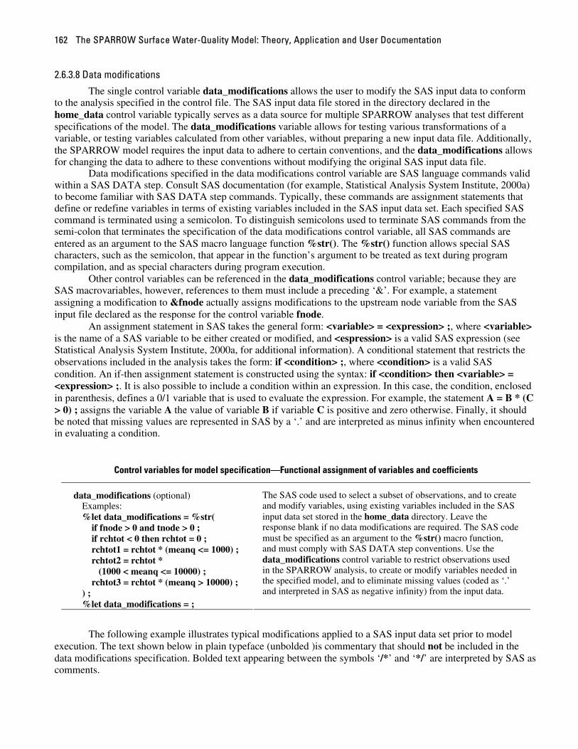
The SPARROW Surface Water-Quality Model: Theory, Application and User Documentation 162
2.6.3.8 Data modifications
The single control variable data_modifications allows the user to modify the SAS input data to conform to the analysis specified in the control file. The SAS input data file stored in the directory declared in the home_data control variable typically serves as a data source for multiple SPARROW analyses that test different specifications of the model. The data_modifications variable allows for testing various transformations of a variable, or testing variables calculated from other variables, without preparing a new input data file. Additionally, the SPARROW model requires the input data to adhere to certain conventions, and the data_modifications allows for changing the data to adhere to these conventions without modifying the original SAS input data file.
Data modifications specified in the data modifications control variable are SAS language commands valid within a SAS DATA step. Consult SAS documentation (for example, Statistical Analysis System Institute, 2000a) to become familiar with SAS DATA step commands. Typically, these commands are assignment statements that define or redefine variables in terms of existing variables included in the SAS input data set. Each specified SAS command is terminated using a semicolon. To distinguish semicolons used to terminate SAS commands from the semi-colon that terminates the specification of the data modifications control variable, all SAS commands are entered as an argument to the SAS macro language function %str(). The %str() function allows special SAS characters, such as the semicolon, that appear in the function’s argument to be treated as text during program compilation, and as special characters during program execution.
Other control variables can be referenced in the data_modifications control variable; because they are SAS macrovariables, however, references to them must include a preceding ‘&’. For example, a statement assigning a modification to &fnode actually assigns modifications to the upstream node variable from the SAS input file declared as the response for the control variable fnode.
An assignment statement in SAS takes the general form: <variable> = <expression> ;, where <variable> is the name of a SAS variable to be either created or modified, and <espression> is a valid SAS expression (see Statistical Analysis System Institute, 2000a, for additional information). A conditional statement that restricts the observations included in the analysis takes the form: if <condition> ;, where <condition> is a valid SAS condition. An if-then assignment statement is constructed using the syntax: if <condition> then <variable> = <expression> ;. It is also possible to include a condition within an expression. In this case, the condition, enclosed in parenthesis, defines a 0/1 variable that is used to evaluate the expression. For example, the statement A = B * (C > 0) ; assigns the variable A the value of variable B if variable C is positive and zero otherwise. Finally, it should be noted that missing values are represented in SAS by a ‘.’ and are interpreted as minus infinity when encountered in evaluating a condition.
Control variables for model specification—Functional assignment of variables and coefficients
data_modifications (optional) Examples: %let data_modifications = %str( if fnode > 0 and tnode > 0 ; if rchtot < 0 then rchtot = 0 ; rchtot1 = rchtot * (meanq <= 1000) ; rchtot2 = rchtot * (1000 < meanq <= 10000) ; rchtot3 = rchtot * (meanq > 10000) ; ) ; %let data_modifications = ;
The SAS code used to select a subset of observations, and to create and modify variables, using existing variables included in the SAS input data set stored in the home_data directory. Leave the response blank if no data modifications are required. The SAS code must be specified as an argument to the %str() macro function, and must comply with SAS DATA step conventions. Use the data_modifications control variable to restrict observations used in the SPARROW analysis, to create or modify variables needed in the specified model, and to eliminate missing values (coded as ‘.’ and interpreted in SAS as negative infinity) from the input data.
The following example illustrates typical modifications applied to a SAS input data set prior to model
execution. The text shown below in plain typeface (unbolded )is commentary that should not be included in the data modifications specification. Bolded text appearing between the symbols ‘/*’ and ‘*/’ are interpreted by SAS as comments.
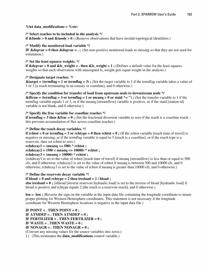
Part 2: SPARROW User’s Guide 163
%let data_modifications = %str(
/* Select reaches to be included in the analysis */ if &fnode > 0 and &tnode > 0 ; (Remove observations that have invalid topological identifiers.)
/* Modify the monitored load variable */ IF &depvar = 0 then &depvar = . ; (Set non-positive monitored loads to missing so that they are not used for estimation.)
/* Set the least squares weights. */ if &depvar > 0 and &ls_weight = . then &ls_weight = 1 ; (Defines a default value for the least squares weights so that each observation with unassigned ls_weight gets equal weight in the analysis.)
/* Designate target reaches. */ &target = (termflag = 1 or termflag = 3) ; (Set the target variable to 1 if the termflag variable takes a value of 1 or 3 [a reach terminating in an estuary or coastline], and 0 otherwise.)
/* Specify the condition for transfer of load from upstream node to downstream node */ &iftran = (termflag = 3 or termflag = 1 or meanq > 0 or staid ^= '') ; (Set the transfer variable to 1 if the termflag variable equals 1 or 3, or if the meanq [streamflow] variable is positive, or if the staid [station id] variable is not blank, and 0 otherwise.)
/* Specify the frac variable for coastline reaches */ if termflag = 3 then &frac = 0 ; (Set the fractional diversion variable to zero if the reach is a coastline reach – this prevents accumulation of flux across coastline reaches.)
/* Define the reach decay variables. */ if rchtot < 0 or termflag = 3 or rchtype = 0 then rchtot = 0 ; (If the rchtot variable [reach time of travel] is negative or missing, or if the termflag variable is equal to 3 [reach is a coastline], or if the reach type is a reservoir, then set rchtot to zero.) rchdecay1 = (meanq <= 500) * rchtot ; rchdecay2 = (500 < meanq <= 10000) * rchtot ; rchdecay3 = (meanq > 10000) * rchtot ; (rchdecay1 is set to the value of rchtot [reach time of travel] if meanq [streamflow] is less than or equal to 500 cfs, and 0 otherwise; rchdecay2 is set to the value of rchtot if meanq is between 500 and 10000 cfs, and 0 otherwise; rchdecay3 is set to the value of rchtot if meanq is greater than 10000 cfs, and 0 otherwise.)
/* Define the reservoir decay variable */ if hload > 0 and rchtype = 2 then iresload = 1 / hload ; else iresload = 0 ; (irhload [inverse reservoir hydraulic load] is set to the inverse of hload [hydraulic load] if hload is positive and rchtype equals 2 [the reach is a reservoir reach], and 0 otherwise.)
lon = -lon ; (Reverse the sign on the variable in the input data file containing the longitude coordinate to insure proper plotting for Western Hemisphere coordinates. This statement is not necessary if the longitude coordinate for Western Hemisphere locations is negative in the input data file.)
IF POINT = . THEN POINT = 0 ; IF ATMDEP = . THEN ATMDEP = 0 ; IF FERTILIZER = . THEN FERTILIZER = 0 ; IF WASTE = . THEN WASTE = 0 ; IF NONAGR = . THEN NONAGR = 0 ; (Convert any missing values for the source variables into zeros.) ) ; (This terminates the data_modifications control variable.)
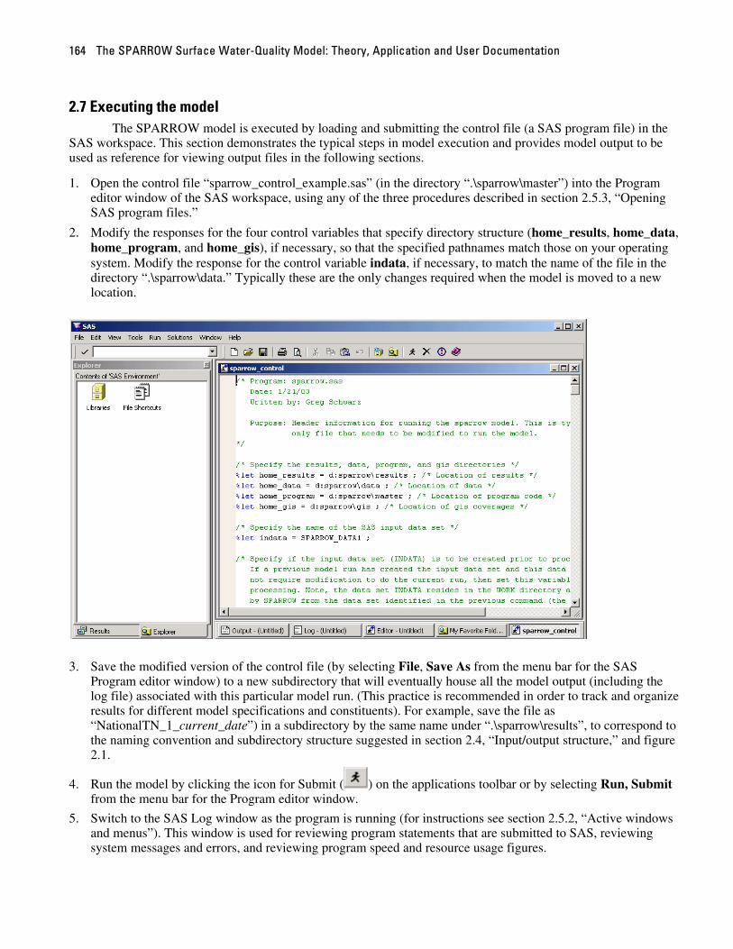
The SPARROW Surface Water-Quality Model: Theory, Application and User Documentation 164
2.7 Executing the model The SPARROW model is executed by loading and submitting the control file (a SAS program file) in the
SAS workspace. This section demonstrates the typical steps in model execution and provides model output to be used as reference for viewing output files in the following sections.
1. Open the control file “sparrow_control_example.sas” (in the directory “.\sparrow\master”) into the Program editor window of the SAS workspace, using any of the three procedures described in section 2.5.3, “Opening SAS program files.”
2. Modify the responses for the four control variables that specify directory structure (home_results, home_data, home_program, and home_gis), if necessary, so that the specified pathnames match those on your operating system. Modify the response for the control variable indata, if necessary, to match the name of the file in the directory “.\sparrow\data.” Typically these are the only changes required when the model is moved to a new location.
3. Save the modified version of the control file (by selecting File, Save As from the menu bar for the SAS Program editor window) to a new subdirectory that will eventually house all the model output (including the log file) associated with this particular model run. (This practice is recommended in order to track and organize results for different model specifications and constituents). For example, save the file as “NationalTN_1_current_date”) in a subdirectory by the same name under “.\sparrow\results”, to correspond to the naming convention and subdirectory structure suggested in section 2.4, “Input/output structure,” and figure 2.1.
4. Run the model by clicking the icon for Submit ( ) on the applications toolbar or by selecting Run, Submit from the menu bar for the Program editor window.
5. Switch to the SAS Log window as the program is running (for instructions see section 2.5.2, “Active windows and menus”). This window is used for reviewing program statements that are submitted to SAS, reviewing system messages and errors, and reviewing program speed and resource usage figures.
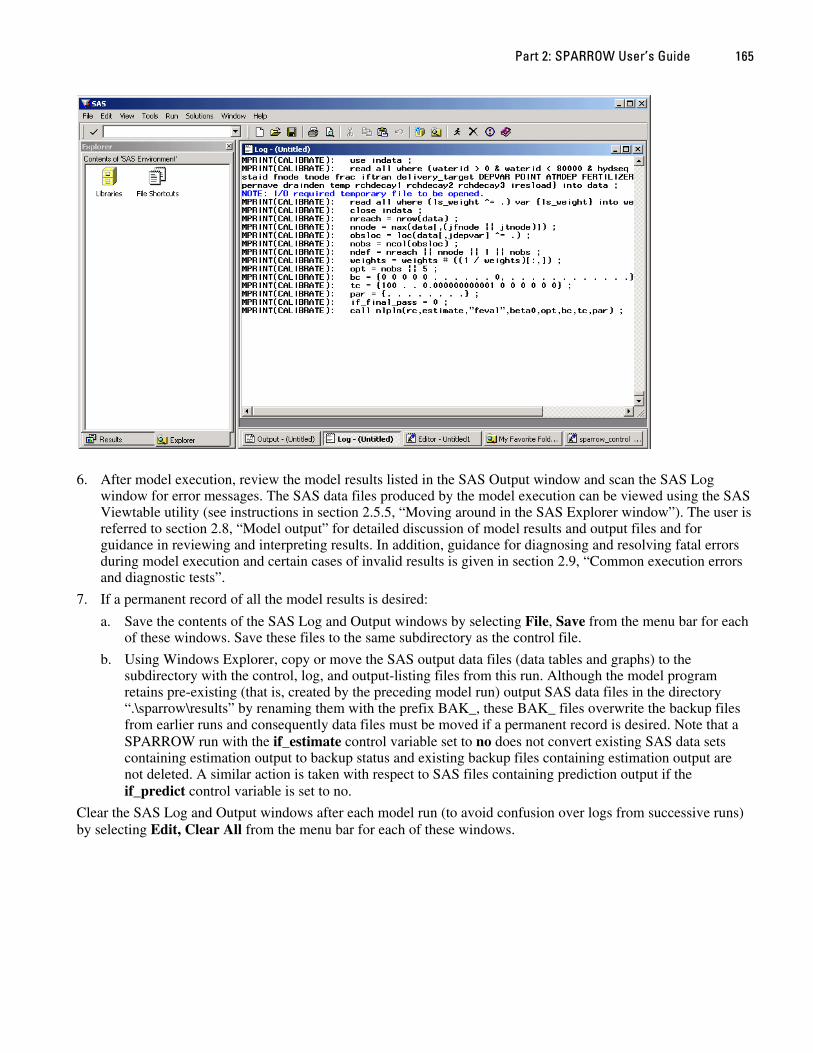
Part 2: SPARROW User’s Guide 165
6. After model execution, review the model results listed in the SAS Output window and scan the SAS Log window for error messages. The SAS data files produced by the model execution can be viewed using the SAS Viewtable utility (see instructions in section 2.5.5, “Moving around in the SAS Explorer window”). The user is referred to section 2.8, “Model output” for detailed discussion of model results and output files and for guidance in reviewing and interpreting results. In addition, guidance for diagnosing and resolving fatal errors during model execution and certain cases of invalid results is given in section 2.9, “Common execution errors and diagnostic tests”.
7. If a permanent record of all the model results is desired:
a. Save the contents of the SAS Log and Output windows by selecting File, Save from the menu bar for each of these windows. Save these files to the same subdirectory as the control file.
b. Using Windows Explorer, copy or move the SAS output data files (data tables and graphs) to the subdirectory with the control, log, and output-listing files from this run. Although the model program retains pre-existing (that is, created by the preceding model run) output SAS data files in the directory “.\sparrow\results” by renaming them with the prefix BAK_, these BAK_ files overwrite the backup files from earlier runs and consequently data files must be moved if a permanent record is desired. Note that a SPARROW run with the if_estimate control variable set to no does not convert existing SAS data sets containing estimation output to backup status and existing backup files containing estimation output are not deleted. A similar action is taken with respect to SAS files containing prediction output if the if_predict control variable is set to no.
Clear the SAS Log and Output windows after each model run (to avoid confusion over logs from successive runs) by selecting Edit, Clear All from the menu bar for each of these windows.

The SPARROW Surface Water-Quality Model: Theory, Application and User Documentation 166
2.8 Model output This section describes and interprets the different forms of SPARROW model output. Output consists of
two separate components, estimation output (for example, coefficients and fit statistics) and prediction output (for example, reach-level predictions). A model run produces output from either or both of these components depending on the responses for the control variables if_estimate and if_predict control variables in the control file.
Each component of the output in turn consists of three forms of output: messages printed to the SAS Log window, tables and graphs listed in the SAS Results and Output windows, and text files and SAS data files written to the “.\sparrow\results” directory. The discussion of estimation output in section 2.8.1 below is organized into four subsections, according to the form of output:
• estimation results listed in the SAS Output window (tables of nonlinear optimizations results and diagnostics, model fit statistics and coefficient estimates),
• graphs listed in the SAS Results window,
• SAS data files containing estimation output,
• text files summarizing the estimation results.
Similarly, the discussion of prediction output in section 2.8.2 is organized into two subsections:
• Summary tables of prediction results listed in the SAS Results and Output windows, and
• SAS data files containing prediction output.
Other output files, described in section 2.8.3, contain output from either estimation or prediction, or both. Finally, estimation and prediction output can be linked, optionally, to SAS/GIS spatial data bases during SPARROW model execution, as described in section 2.8.4.
Messages printed to the SAS Log window are of interest for tracking the source of any errors that occurred during a SPARROW program execution. A brief inspection of the SAS Log window following a model run therefore should be common practice. Even if detailed printing to the SAS Log window is turned off (if the control variable if_print_details in the control file is set to no), messages pertaining to execution errors are printed to the Log window.
The elements (tables) in the SAS Output window after a model run can also be accessed through the tree structure in the SAS Results window. To view specific output tables or graphs, double-click the corresponding entry in the SAS Results window.
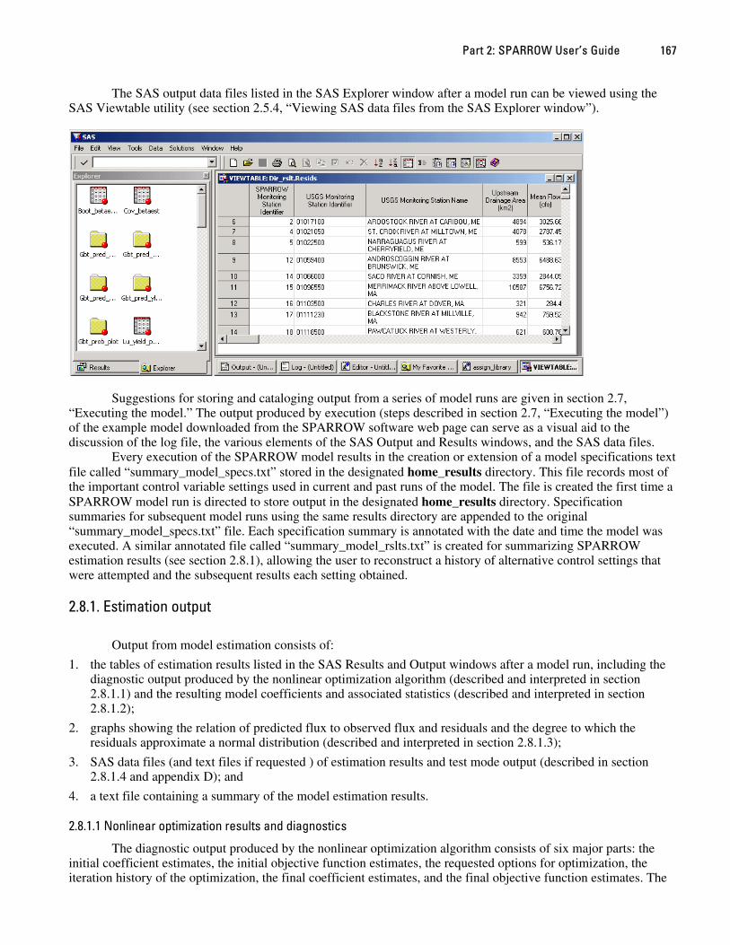
Part 2: SPARROW User’s Guide 167
The SAS output data files listed in the SAS Explorer window after a model run can be viewed using the SAS Viewtable utility (see section 2.5.4, “Viewing SAS data files from the SAS Explorer window”).
Suggestions for storing and cataloging output from a series of model runs are given in section 2.7,
“Executing the model.” The output produced by execution (steps described in section 2.7, “Executing the model”) of the example model downloaded from the SPARROW software web page can serve as a visual aid to the discussion of the log file, the various elements of the SAS Output and Results windows, and the SAS data files.
Every execution of the SPARROW model results in the creation or extension of a model specifications text file called “summary_model_specs.txt” stored in the designated home_results directory. This file records most of the important control variable settings used in current and past runs of the model. The file is created the first time a SPARROW model run is directed to store output in the designated home_results directory. Specification summaries for subsequent model runs using the same results directory are appended to the original “summary_model_specs.txt” file. Each specification summary is annotated with the date and time the model was executed. A similar annotated file called “summary_model_rslts.txt” is created for summarizing SPARROW estimation results (see section 2.8.1), allowing the user to reconstruct a history of alternative control settings that were attempted and the subsequent results each setting obtained.
2.8.1. Estimation output
Output from model estimation consists of:
1. the tables of estimation results listed in the SAS Results and Output windows after a model run, including the diagnostic output produced by the nonlinear optimization algorithm (described and interpreted in section 2.8.1.1) and the resulting model coefficients and associated statistics (described and interpreted in section 2.8.1.2);
2. graphs showing the relation of predicted flux to observed flux and residuals and the degree to which the residuals approximate a normal distribution (described and interpreted in section 2.8.1.3);
3. SAS data files (and text files if requested ) of estimation results and test mode output (described in section 2.8.1.4 and appendix D); and
4. a text file containing a summary of the model estimation results.
2.8.1.1 Nonlinear optimization results and diagnostics
The diagnostic output produced by the nonlinear optimization algorithm consists of six major parts: the initial coefficient estimates, the initial objective function estimates, the requested options for optimization, the iteration history of the optimization, the final coefficient estimates, and the final objective function estimates. The
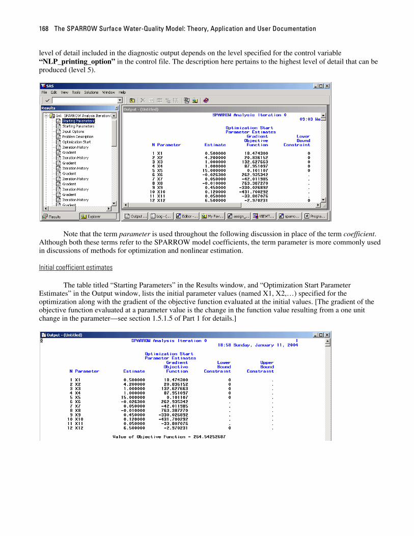
The SPARROW Surface Water-Quality Model: Theory, Application and User Documentation 168
level of detail included in the diagnostic output depends on the level specified for the control variable “NLP_printing_option” in the control file. The description here pertains to the highest level of detail that can be produced (level 5).
Note that the term parameter is used throughout the following discussion in place of the term coefficient.
Although both these terms refer to the SPARROW model coefficients, the term parameter is more commonly used in discussions of methods for optimization and nonlinear estimation.
Initial coefficient estimates
The table titled “Starting Parameters” in the Results window, and “Optimization Start Parameter Estimates” in the Output window, lists the initial parameter values (named X1, X2,…) specified for the optimization along with the gradient of the objective function evaluated at the initial values. [The gradient of the objective function evaluated at a parameter value is the change in the function value resulting from a one unit change in the parameter—see section 1.5.1.5 of Part 1 for details.]
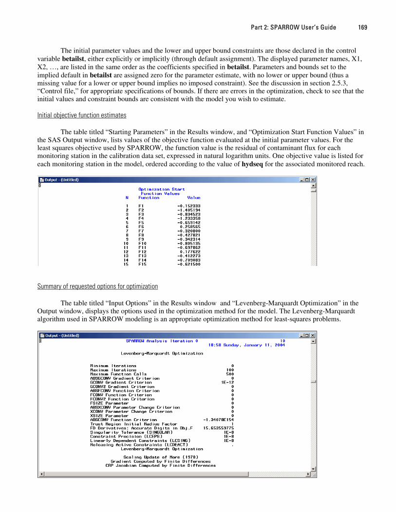
Part 2: SPARROW User’s Guide 169
The initial parameter values and the lower and upper bound constraints are those declared in the control variable betailst, either explicitly or implicitly (through default assignment). The displayed parameter names, X1, X2, …, are listed in the same order as the coefficients specified in betailst. Parameters and bounds set to the implied default in betailst are assigned zero for the parameter estimate, with no lower or upper bound (thus a missing value for a lower or upper bound implies no imposed constraint). See the discussion in section 2.5.3, “Control file,” for appropriate specifications of bounds. If there are errors in the optimization, check to see that the initial values and constraint bounds are consistent with the model you wish to estimate. Initial objective function estimates
The table titled “Starting Parameters” in the Results window, and “Optimization Start Function Values” in the SAS Output window, lists values of the objective function evaluated at the initial parameter values. For the least squares objective used by SPARROW, the function value is the residual of contaminant flux for each monitoring station in the calibration data set, expressed in natural logarithm units. One objective value is listed for each monitoring station in the model, ordered according to the value of hydseq for the associated monitored reach.
Summary of requested options for optimization
The table titled “Input Options” in the Results window and “Levenberg-Marquardt Optimization” in the Output window, displays the options used in the optimization method for the model. The Levenberg-Marquardt algorithm used in SPARROW modeling is an appropriate optimization method for least-squares problems.

The SPARROW Surface Water-Quality Model: Theory, Application and User Documentation 170
The first 14 options displayed in the table (through ABSCONV Function Criterion) pertain to termination criteria used by SAS. The first three of these options define limits on the algorithm that, if exceeded, constitute an abnormal termination of the algorithm. The maximum number of iterations is set to 100, which far exceeds the 10-20 iterations typically required to achieve convergence for a SPARROW model. Generally, failure to converge within 100 iterations indicates an error in the model specification. The maximum function calls, set at 500, defines the maximum number of times the objective function is evaluated. This number should be greater than the number of iterations because multiple function calls are required for each iteration to determine numerical gradients (that is, changes in the objective with respect to changes in the parameter values) used for evaluating the step change in parameter values between iterations (see section 1.5.1.5 in Part 1). The maximum limit for function calls should not be set too high, however; setting a limit which far exceeds the limit for iterations could result in unnecessarily long execution times (each evaluation of the objective function requires a complete pass through the reach network) prior to determining that the algorithm is not converging, an indication of a problem in model specification.
The remaining 11 termination criteria pertain to conditions for convergence of the algorithm (see Statistical Analysis System Institute, 2000b, for documentation of the different criteria). A zero value for a setting effectively disables that particular criterion. The SPARROW model is configured to terminate based on convergence of the relative gradients (GCONV) criterion. This criterion is evaluated by pre- and post-multiplying the inverse of the Hessian matrix by the gradient vectors, and normalizing the result by the value of the objective function. Note, however, that a SPARROW model may converge on the basis of other criteria; for example, if successive values of the objective function across iterations show no change. In this case, the solution is deemed within the noise of the numerical precision of the estimated objective function, so convergence is assumed. The item defining FD Derivatives refers to the number of digits accuracy applied to the objective function in computing numerical, finite difference derivatives. SPARROW uses forward difference approximations to the derivatives of the objective function with respect to the model coefficients. (A more accurate approximation is central differences but this requires more evaluations of the objective function at each iteration.) The remaining items pertain to the precision with which SAS tests the solution for singularity of the Hessian matrix and imposition of active constraints on the estimated coefficients.
Iteration history
The iteration history gives details on progress towards convergence for each iteration of the optimization algorithm. For each iteration, SAS reports the values and gradients for each parameter (listed in the same order as specified in the control variable betailst in the control file), the value of the objective function evaluated at the parameter values shown, as well as information on the number of function calls required to complete the iteration and any active constraints associated with the parameter values. A well-specified SPARROW model should show steady progress towards convergence, with the gradients of unconstrained coefficients going to zero.
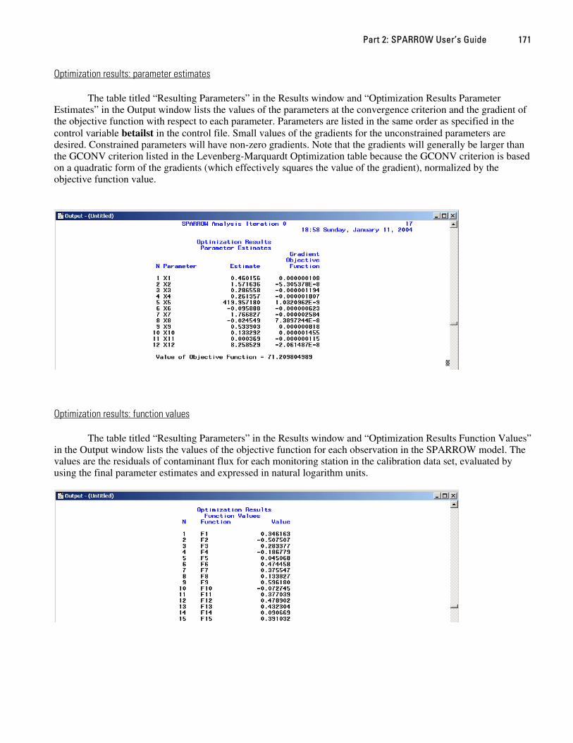
Part 2: SPARROW User’s Guide 171
Optimization results: parameter estimates
The table titled “Resulting Parameters” in the Results window and “Optimization Results Parameter Estimates” in the Output window lists the values of the parameters at the convergence criterion and the gradient of the objective function with respect to each parameter. Parameters are listed in the same order as specified in the control variable betailst in the control file. Small values of the gradients for the unconstrained parameters are desired. Constrained parameters will have non-zero gradients. Note that the gradients will generally be larger than the GCONV criterion listed in the Levenberg-Marquardt Optimization table because the GCONV criterion is based on a quadratic form of the gradients (which effectively squares the value of the gradient), normalized by the objective function value.
Optimization results: function values
The table titled “Resulting Parameters” in the Results window and “Optimization Results Function Values” in the Output window lists the values of the objective function for each observation in the SPARROW model. The values are the residuals of contaminant flux for each monitoring station in the calibration data set, evaluated by using the final parameter estimates and expressed in natural logarithm units.
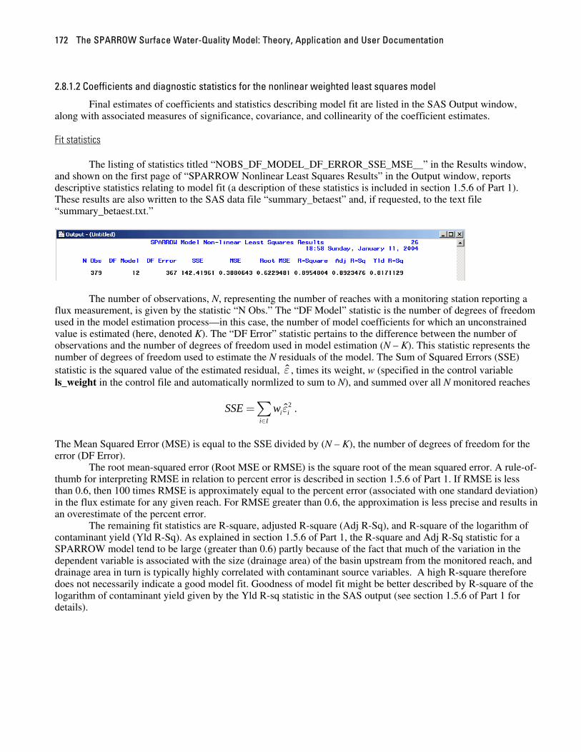
The SPARROW Surface Water-Quality Model: Theory, Application and User Documentation 172
2.8.1.2 Coefficients and diagnostic statistics for the nonlinear weighted least squares model
Final estimates of coefficients and statistics describing model fit are listed in the SAS Output window, along with associated measures of significance, covariance, and collinearity of the coefficient estimates.
Fit statistics
The listing of statistics titled “NOBS_DF_MODEL_DF_ERROR_SSE_MSE__” in the Results window, and shown on the first page of “SPARROW Nonlinear Least Squares Results” in the Output window, reports descriptive statistics relating to model fit (a description of these statistics is included in section 1.5.6 of Part 1). These results are also written to the SAS data file “summary_betaest” and, if requested, to the text file “summary_betaest.txt.”
The number of observations, N, representing the number of reaches with a monitoring station reporting a flux measurement, is given by the statistic “N Obs.” The “DF Model” statistic is the number of degrees of freedom used in the model estimation process—in this case, the number of model coefficients for which an unconstrained value is estimated (here, denoted K). The “DF Error” statistic pertains to the difference between the number of observations and the number of degrees of freedom used in model estimation (N – K). This statistic represents the number of degrees of freedom used to estimate the N residuals of the model. The Sum of Squared Errors (SSE) statistic is the squared value of the estimated residual, , times its weight, w (specified in the control variable ls_weight in the control file and automatically normlized to sum to N), and summed over all N monitored reaches
ε
. 2ˆi ii I
SSE w ε∈
=∑
The Mean Squared Error (MSE) is equal to the SSE divided by (N – K), the number of degrees of freedom for the error (DF Error).
The root mean-squared error (Root MSE or RMSE) is the square root of the mean squared error. A rule-of-thumb for interpreting RMSE in relation to percent error is described in section 1.5.6 of Part 1. If RMSE is less than 0.6, then 100 times RMSE is approximately equal to the percent error (associated with one standard deviation) in the flux estimate for any given reach. For RMSE greater than 0.6, the approximation is less precise and results in an overestimate of the percent error.
The remaining fit statistics are R-square, adjusted R-square (Adj R-Sq), and R-square of the logarithm of contaminant yield (Yld R-Sq). As explained in section 1.5.6 of Part 1, the R-square and Adj R-Sq statistic for a SPARROW model tend to be large (greater than 0.6) partly because of the fact that much of the variation in the dependent variable is associated with the size (drainage area) of the basin upstream from the monitored reach, and drainage area in turn is typically highly correlated with contaminant source variables. A high R-square therefore does not necessarily indicate a good model fit. Goodness of model fit might be better described by R-square of the logarithm of contaminant yield given by the Yld R-sq statistic in the SAS output (see section 1.5.6 of Part 1 for details).
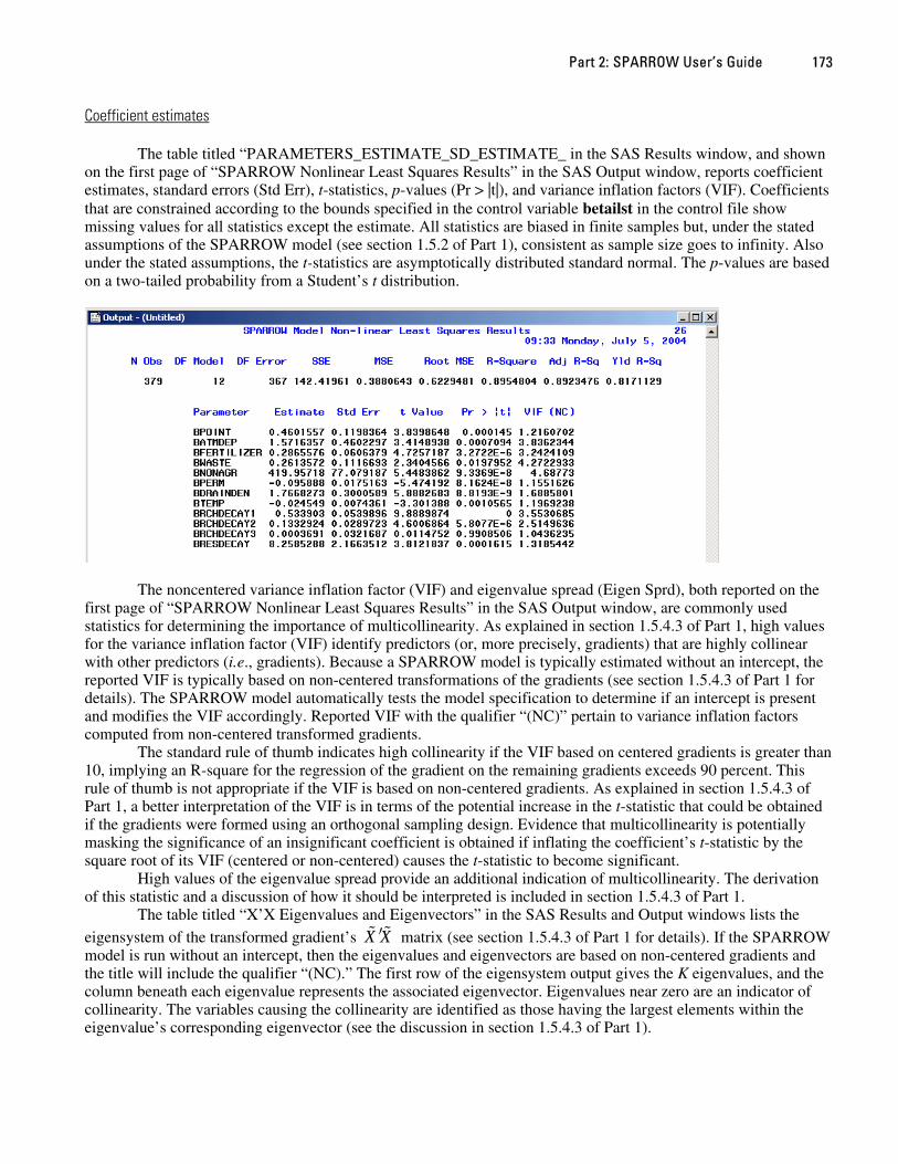
Part 2: SPARROW User’s Guide 173
Coefficient estimates
The table titled “PARAMETERS_ESTIMATE_SD_ESTIMATE_ in the SAS Results window, and shown on the first page of “SPARROW Nonlinear Least Squares Results” in the SAS Output window, reports coefficient estimates, standard errors (Std Err), t-statistics, p-values (Pr > |t|), and variance inflation factors (VIF). Coefficients that are constrained according to the bounds specified in the control variable betailst in the control file show missing values for all statistics except the estimate. All statistics are biased in finite samples but, under the stated assumptions of the SPARROW model (see section 1.5.2 of Part 1), consistent as sample size goes to infinity. Also under the stated assumptions, the t-statistics are asymptotically distributed standard normal. The p-values are based on a two-tailed probability from a Student’s t distribution.
The noncentered variance inflation factor (VIF) and eigenvalue spread (Eigen Sprd), both reported on the first page of “SPARROW Nonlinear Least Squares Results” in the SAS Output window, are commonly used statistics for determining the importance of multicollinearity. As explained in section 1.5.4.3 of Part 1, high values for the variance inflation factor (VIF) identify predictors (or, more precisely, gradients) that are highly collinear with other predictors (i.e., gradients). Because a SPARROW model is typically estimated without an intercept, the reported VIF is typically based on non-centered transformations of the gradients (see section 1.5.4.3 of Part 1 for details). The SPARROW model automatically tests the model specification to determine if an intercept is present and modifies the VIF accordingly. Reported VIF with the qualifier “(NC)” pertain to variance inflation factors computed from non-centered transformed gradients.
The standard rule of thumb indicates high collinearity if the VIF based on centered gradients is greater than 10, implying an R-square for the regression of the gradient on the remaining gradients exceeds 90 percent. This rule of thumb is not appropriate if the VIF is based on non-centered gradients. As explained in section 1.5.4.3 of Part 1, a better interpretation of the VIF is in terms of the potential increase in the t-statistic that could be obtained if the gradients were formed using an orthogonal sampling design. Evidence that multicollinearity is potentially masking the significance of an insignificant coefficient is obtained if inflating the coefficient’s t-statistic by the square root of its VIF (centered or non-centered) causes the t-statistic to become significant.
High values of the eigenvalue spread provide an additional indication of multicollinearity. The derivation of this statistic and a discussion of how it should be interpreted is included in section 1.5.4.3 of Part 1.
The table titled “X’X Eigenvalues and Eigenvectors” in the SAS Results and Output windows lists the
eigensystem of the transformed gradient’s X X′ matrix (see section 1.5.4.3 of Part 1 for details). If the SPARROW model is run without an intercept, then the eigenvalues and eigenvectors are based on non-centered gradients and the title will include the qualifier “(NC).” The first row of the eigensystem output gives the K eigenvalues, and the column beneath each eigenvalue represents the associated eigenvector. Eigenvalues near zero are an indicator of collinearity. The variables causing the collinearity are identified as those having the largest elements within the eigenvalue’s corresponding eigenvector (see the discussion in section 1.5.4.3 of Part 1).
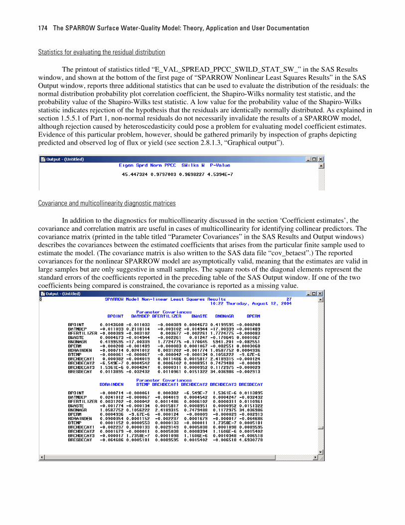
The SPARROW Surface Water-Quality Model: Theory, Application and User Documentation 174
Statistics for evaluating the residual distribution
The printout of statistics titled “E_VAL_SPREAD_PPCC_SWILD_STAT_SW_” in the SAS Results window, and shown at the bottom of the first page of “SPARROW Nonlinear Least Squares Results” in the SAS Output window, reports three additional statistics that can be used to evaluate the distribution of the residuals: the normal distribution probability plot correlation coefficient, the Shapiro-Wilks normality test statistic, and the probability value of the Shapiro-Wilks test statistic. A low value for the probability value of the Shapiro-Wilks statistic indicates rejection of the hypothesis that the residuals are identically normally distributed. As explained in section 1.5.5.1 of Part 1, non-normal residuals do not necessarily invalidate the results of a SPARROW model, although rejection caused by heteroscedasticity could pose a problem for evaluating model coefficient estimates. Evidence of this particular problem, however, should be gathered primarily by inspection of graphs depicting predicted and observed log of flux or yield (see section 2.8.1.3, “Graphical output”).
Covariance and multicollinearity diagnostic matrices
In addition to the diagnostics for multicollinearity discussed in the section ‘Coefficient estimates’, the covariance and correlation matrix are useful in cases of multicollinearity for identifying collinear predictors. The covariance matrix (printed in the table titled “Parameter Covariances” in the SAS Results and Output windows) describes the covariances between the estimated coefficients that arises from the particular finite sample used to estimate the model. (The covariance matrix is also written to the SAS data file “cov_betaest”.) The reported covariances for the nonlinear SPARROW model are asymptotically valid, meaning that the estimates are valid in large samples but are only suggestive in small samples. The square roots of the diagonal elements represent the standard errors of the coefficients reported in the preceding table of the SAS Output window. If one of the two coefficients being compared is constrained, the covariance is reported as a missing value.

Part 2: SPARROW User’s Guide 175
Because covariances are somewhat difficult to interpret, SPARROW also reports the correlation matrix (titled “Parameter Correlations” in the SAS Results and Output windows). An element in the correlation matrix represents the correlation between two estimated coefficients. The element given in the ith row and jth column is computed by taking the covariance between the ith and jth coefficients and dividing by the square root of the product of the variances for the ith and jth coefficients. As with correlations in general, the elements of this matrix must lie between –1 and 1. Because a coefficient estimate is perfectly correlated with itself, the elements along the diagonal are set to 1. Correlations of constrained coefficients are reported as missing values. The correlation matrix can be useful in identifying the bivariate case of multicollinearity—that is, collinearity between only two predictors. See section 1.5.4.3 of Part 1 for further discussion.
2.8.1.3 Graphical output
Each model run produces graphs of observed, predicted, and residual values of the dependent variable for the calibration data set, and saves the graphs in the “.\sparrow\results” directory as SAS data sets (catalogs) (described in section 2.8.1.4, “Estimation output files”). The graphs can be viewed by clicking on the SAS catalog name (“gbt_graphname”) listed in a Windows Explorer window, or by double-clicking the “Gplot” entries in the SAS Results window.
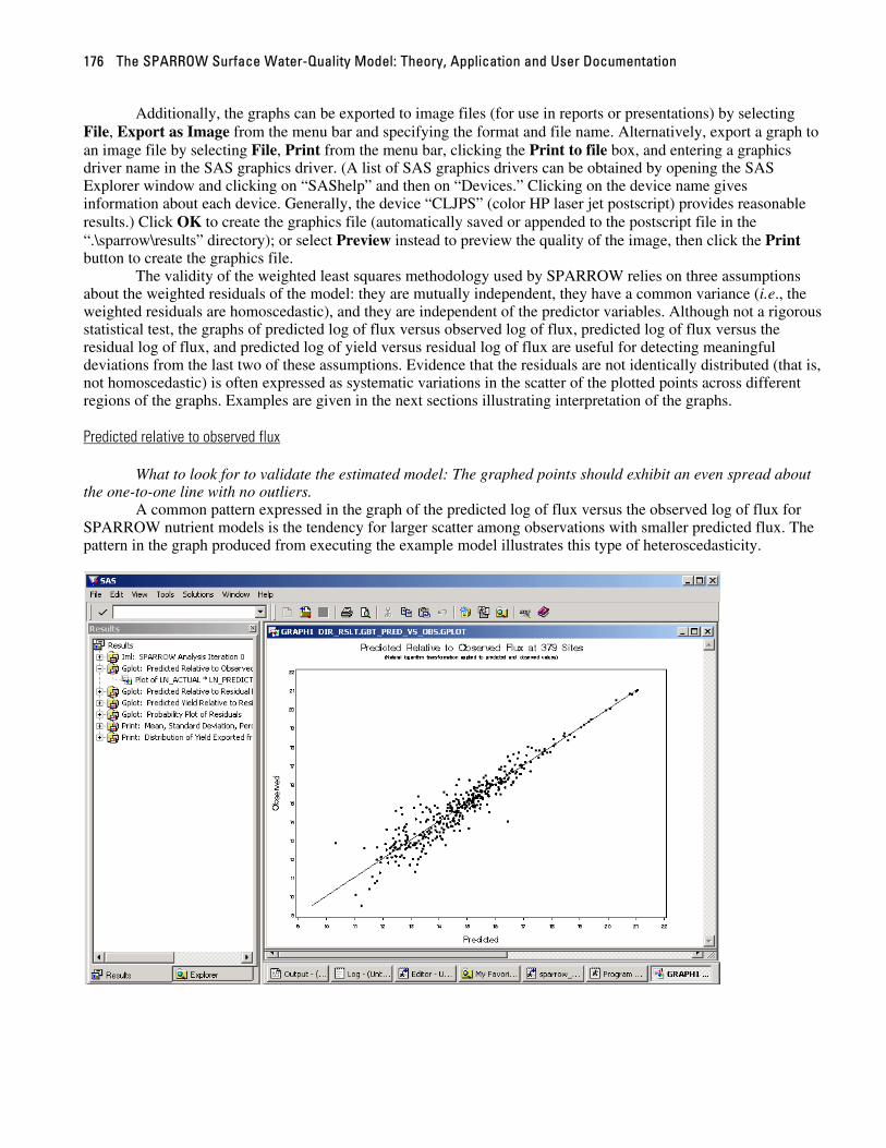
The SPARROW Surface Water-Quality Model: Theory, Application and User Documentation 176
Additionally, the graphs can be exported to image files (for use in reports or presentations) by selecting File, Export as Image from the menu bar and specifying the format and file name. Alternatively, export a graph to an image file by selecting File, Print from the menu bar, clicking the Print to file box, and entering a graphics driver name in the SAS graphics driver. (A list of SAS graphics drivers can be obtained by opening the SAS Explorer window and clicking on “SAShelp” and then on “Devices.” Clicking on the device name gives information about each device. Generally, the device “CLJPS” (color HP laser jet postscript) provides reasonable results.) Click OK to create the graphics file (automatically saved or appended to the postscript file in the “.\sparrow\results” directory); or select Preview instead to preview the quality of the image, then click the Print button to create the graphics file.
The validity of the weighted least squares methodology used by SPARROW relies on three assumptions about the weighted residuals of the model: they are mutually independent, they have a common variance (i.e., the weighted residuals are homoscedastic), and they are independent of the predictor variables. Although not a rigorous statistical test, the graphs of predicted log of flux versus observed log of flux, predicted log of flux versus the residual log of flux, and predicted log of yield versus residual log of flux are useful for detecting meaningful deviations from the last two of these assumptions. Evidence that the residuals are not identically distributed (that is, not homoscedastic) is often expressed as systematic variations in the scatter of the plotted points across different regions of the graphs. Examples are given in the next sections illustrating interpretation of the graphs.
Predicted relative to observed flux
What to look for to validate the estimated model: The graphed points should exhibit an even spread about the one-to-one line with no outliers.
A common pattern expressed in the graph of the predicted log of flux versus the observed log of flux for SPARROW nutrient models is the tendency for larger scatter among observations with smaller predicted flux. The pattern in the graph produced from executing the example model illustrates this type of heteroscedasticity.
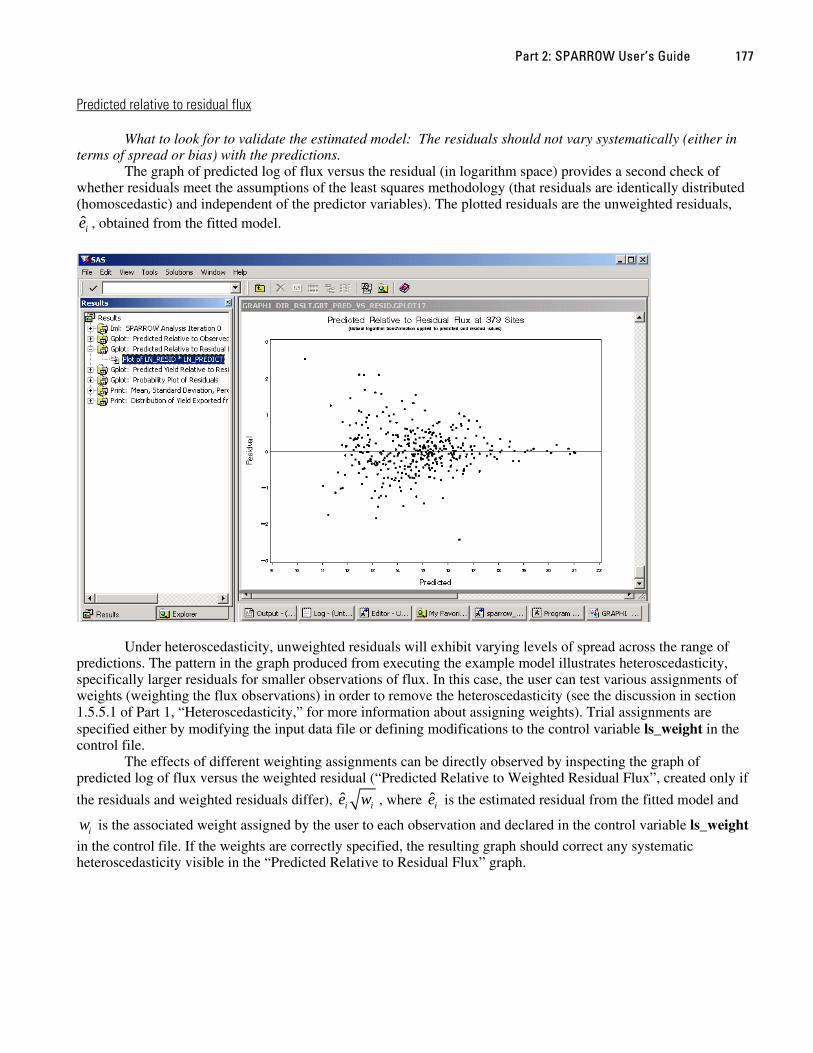
Part 2: SPARROW User’s Guide 177
Predicted relative to residual flux
What to look for to validate the estimated model: The residuals should not vary systematically (either in terms of spread or bias) with the predictions.
The graph of predicted log of flux versus the residual (in logarithm space) provides a second check of whether residuals meet the assumptions of the least squares methodology (that residuals are identically distributed (homoscedastic) and independent of the predictor variables). The plotted residuals are the unweighted residuals,
, obtained from the fitted model. ie
Under heteroscedasticity, unweighted residuals will exhibit varying levels of spread across the range of predictions. The pattern in the graph produced from executing the example model illustrates heteroscedasticity, specifically larger residuals for smaller observations of flux. In this case, the user can test various assignments of weights (weighting the flux observations) in order to remove the heteroscedasticity (see the discussion in section 1.5.5.1 of Part 1, “Heteroscedasticity,” for more information about assigning weights). Trial assignments are specified either by modifying the input data file or defining modifications to the control variable ls_weight in the control file.
The effects of different weighting assignments can be directly observed by inspecting the graph of predicted log of flux versus the weighted residual (“Predicted Relative to Weighted Residual Flux”, created only if
the residuals and weighted residuals differ), ie wi , where is the estimated residual from the fitted model and
is the associated weight assigned by the user to each observation and declared in the control variable ls_weight
in the control file. If the weights are correctly specified, the resulting graph should correct any systematic heteroscedasticity visible in the “Predicted Relative to Residual Flux” graph.
ie
iw

The SPARROW Surface Water-Quality Model: Theory, Application and User Documentation 178
Predicted yield relative to residual flux
What to look for to validate the estimated model: The residuals should not vary systematically (either in terms of spread or bias) with the prediction; a systematic pattern indicates misspecification of the model at the watershed scale.
The plot of predicted log of yield versus the residual log of flux, or weighted residual log of flux if the model is estimated with weights that vary across observations, can be used to determine if there are any systematic relations between the predictors and the residuals (that is, failure of the assumption that residuals are independent of predictors) that transcend scale effects. Observation of a systematic pattern in this plot indicates that the model is misspecified, and further indicates, as a pattern observed on this plot would not be due to scale effects, that the likely source of the misspecification is the land-to-water delivery process or the omission of an important source variable. Conversely, if a systematic pattern is not observed on this plot, but is observed between the weighted residuals and predicted flux (see previous discussion of “Predicted Relative to Residual Flux”), then it can be concluded that misspecification of the model is likely related to processes that accumulate flux across different scales.
Probability plot of residuals
What to look for: normally distributed weighted residuals will plot along the reference line (departure from this condition does not, however, necessarily invalidate the estimated model).
The probability plot depicts the relation between the empirical distribution of the residuals and the normal distribution. Specifically, it is the scatter plot relating the ordered standardized weighted residuals, and the
quantiles of the adjusted ranks (see the discussion of the probability plot correlation coefficient in section
1.5.5.1 of Part 1). If the weighted residuals are approximately normally distributed, and the probability plot correlation coefficient is near one, the points should plot along the one-to-one line. (The one-to-one line corresponds to the line formed by the mean of e* plus the standard deviation of e* times the minimum and maximum values of e*.) If the probability plot correlation coefficient is considerably less than one, on the other hand, the points will deviate from the one-to-one line. In the latter case, further interpretation of the graph can indicate the nature of the deviation from normality (see section 1.5.5.1 of Part 1 for additional details).
ie∗
iq
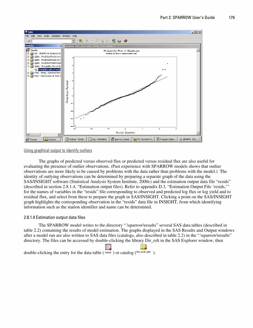
Part 2: SPARROW User’s Guide 179
Using graphical output to identify outliers
The graphs of predicted versus observed flux or predicted versus residual flux are also useful for evaluating the presence of outlier observations. (Past experience with SPARROW models shows that outlier observations are more likely to be caused by problems with the data rather than problems with the model.) The identity of outlying observations can be determined by preparing a separate graph of the data using the SAS/INSIGHT software (Statistical Analysis System Institute, 2000c) and the estimation output data file “resids” (described in section 2.8.1.4, “Estimation output files). Refer to appendix D.3, “Estimation Output File ‘resids,’” for the names of variables in the “resids” file corresponding to observed and predicted log flux or log yield and to residual flux, and select from these to prepare the graph in SAS/INSIGHT. Clicking a point on the SAS/INSIGHT graph highlights the corresponding observation in the “resids” data file in INSIGHT, from which identifying information such as the station identifier and name can be determined.
2.8.1.4 Estimation output data files
The SPARROW model writes to the directory “.\sparrow\results” several SAS data tables (described in table 2.2) containing the results of model estimation. The graphs displayed in the SAS Results and Output windows after a model run are also written to SAS data files (catalogs, also described in table 2.2) in the “.\sparrow\results” directory. The files can be accessed by double-clicking the library Dir_rslt in the SAS Explorer window, then
double-clicking the entry for the data table ( ) or catalog ( ).
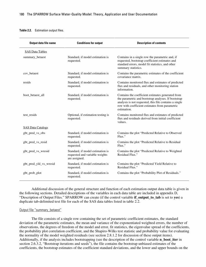
The SPARROW Surface Water-Quality Model: Theory, Application and User Documentation 180
Table 2.2. Estimation output files.
Output data file name Conditions for output Description of contents
SAS Data Tables
summary_betaest Standard, if model estimation is requested.
Contains in a single row the parametric and, if requested, bootstrap coefficient estimates and standard errors, model fit statistics, and other summary statistics.
cov_betaest Standard, if model estimation is requested.
Contains the parametric estimates of the coefficient covariance matrix.
resids Standard, if model estimation is requested.
Contains monitored flux and estimates of predicted flux and residuals, and other monitoring station information.
boot_betaest_all Standard, if model estimation is requested.
Contains the coefficient estimates generated from the parametric and bootstrap analyses. If bootstrap analysis is not requested, this file contains a single row with coefficient estimates from parametric estimation.
test_resids Optional, if estimation testing is requested.
Contains monitored flux and estimates of predicted flux and residuals derived from initial coefficient values.
SAS Data Catalogs
gbt_pred_vs_obs Standard, if model estimation is requested.
Contains the plot “Predicted Relative to Observed Flux.”
gbt_pred_vs_resid Standard, if model estimation is requested.
Contains the plot “Predicted Relative to Residual Flux.”
gbt_pred_vs_wresid Standard, if model estimation is requested and variable weights are assigned.
Contains the plot “Predicted Relative to Weighted Residual Flux.”
gbt_pred_yld_vs_wresid Standard, if model estimation is requested.
Contains the plot “Predicted Yield Relative to Residual Flux.”
gbt_prob_plot Standard, if model estimation is requested.
Contains the plot “Probability Plot of Residuals.”
Additional discussion of the general structure and function of each estimation output data table is given in
the following sections. Detailed descriptions of the variables in each data table are included in appendix D, “Description of Output Files.” SPARROW can create (if the control variable if_output_to_tab is set to yes) a duplicate tab-delimited text file for each of the SAS data tables listed in table 2.2.
Output file “summary_betaest”
The file consists of a single row containing the set of parametric coefficient estimates, the standard deviation of the parametric estimates, the mean and variance of the exponentiated weighted errors, the number of observations, the degrees of freedom of the model and error, fit statistics, the eigenvalue spread of the coefficients, the probability plot correlation coefficient, and the Shapiro-Wilks test statistic and probability value for evaluating the normality of the model weighted residuals (see section 2.8.1.2 for discussion of these output items). Additionally, if the analysis includes bootstrapping (see the description of the control variable n_boot_iter in section 2.6.3.2, “Bootstrap iterations and seeds”), the file contains the bootstrap unbiased estimates of the coefficients, the bootstrap estimates of the coefficient standard deviations, and the lower and upper bounds on the
Part 2: SPARROW User’s Guide 181
bootstrap-defined confidence interval (see section 1.5.3.3 of Part 1 for an explanation of the bootstrap estimates). Note that if a parametric bootstrap has been specified (see the description of the control variable if_parm_bootstrap in section 2.6.3.7, “Options for model execution”), the bootstrap estimates will closely match the parametric equivalents. Appendix D.1, “Estimation Output File ‘summary_betaest,’” contains detailed descriptions of each variable in this file.
Output file “cov_betaest”
The file contains the covariance matrix, variance inflation factors and eigenvalues for the SPARROW model parametric coefficient estimates (see section 1.5.4.3 of Part 1 for a discussion of the interpretation of the variance inflation factors and eigenvalues). The number of observations in this file equals the number of coefficients in the model. The order of the coefficients across the rows and columns is the same as that specified in the control variable betailst in the control file. Appendix D.2, “Estimation Output File ‘cov_betaest,’” contains detailed descriptions of each variable in this file.
Output file “resids”
The file contains the ancillary information about each monitoring station, the station weight used for computing weighted least squares, measured and predicted flux in both real and natural logarithm units, various transformations of the model residuals, the observation’s leverage, and the gradients associated with the model coefficients. Many of the variables used in the graphs described in section 2.8.1.3, “Graphical output,” are included in the “resids” file. Appendix D.3, “Estimation Output File ‘resids,’” contains detailed descriptions of each variable in this file. The tab-delimited text file version of this file is particularly useful for transporting station results to ArcView in order to produce spatial plots of the residuals.
Output file “boot_betaest_all”
This file contains the coefficient estimates for each bootstrap iteration. The first observation pertains to coefficient estimates from the parametric model. Subsequent observations pertain to the bootstrap iteration estimates. The file is created even if a bootstrap analysis is not requested, and in this case contains a single row with the parametric estimates. Appendix D.4, “Estimation Output File ‘boot_betaest,’” contains detailed descriptions of each variable in this file.
If a parametric bootstrap has been specified (see the description of the control variable if_parm_bootstrap in section 2.6.3.7, “Options for model execution”), the coefficient estimates for the bootstrap iterations are generated using a normal random number generator with the set of bootstrap coefficients in the rth iteration given by
, ˆ ˆr rb b Pz= +
where is the k-element vector of parametric coefficient estimates, P is a k × k matrix representing the Cholesky
decomposition of the parametric estimates’ covariance matrix (that is,
b
( )ˆV b ( )ˆVPP b′ = ), and is a k-element
vector corresponding to the r
rzth iteration’s random draw from a independent standard normal distribution. If the
parametric bootstrap is not selected, then the bootstrap coefficient estimates are obtained by reestimating the SPARROW model using random weights (see section 1.5.3.1 of Part 1). The number of observations (rows) in the file “boot_betaest_all” equals the number of bootstrap iterations performed plus one, the additional observation representing the parametric estimates.

The SPARROW Surface Water-Quality Model: Theory, Application and User Documentation 182
Output file “test_resids” (optional)
This file contains output from the estimation algorithm in test mode. The file is created only if the control variables if_estimate and if_test_calibrate in the control file are both set to yes, in which case the estimation test output supplants the creation of all other SPARROW estimation output. The contents of the file “test_resids” can be used to determine if any monitored reaches have negative values of predicted flux (the variable PREDICT). Instances of negative flux require a modification of the model—either by changing the included variables, modifying the process specifications, or imposing additional bounds on the coefficients. All values of the predictions and residuals reported in the file “test_resids” are obtained using the initial values of the coefficients as specified in the control variable betailst. See additional discussion in section 2.9.2.2, “Estimation execution errors caused by numerical overflow—using the test-calibration mode”; a description of the variables in the test_resids data set is contained in appendix D.5, “Estimation Output File ‘test_resids.’”
2.8.1.5 Summary estimation output
In order to assist the user in organizing output from multiple model runs, SPARROW produces summary files that record the options selected for each model run and, if model estimation is performed, a summary of the weighted nonlinear least squares estimation results. The summary estimation results from multiple runs of the model are stored in the text file “summary_model_rslts.txt” stored in the home_results directory. The summary file is created the first time a SPARROW model directs estimation results to the home_results directory. Estimation results from subsequent model runs are appended to the file and annotated with respect to the date and time the model was run. The annotation permits the user to correlate the estimation results with the model control specifications for that run as recorded in the “summary_model_specs.txt” file.
The summary file includes all the fit statistics, coefficient estimates and associated standard errors, t-statistics and p-values, variance inflation factors, eigenvalue spread, Shapiro-Wilks test statistic and significance level, and probability plot correlation coefficient. Additionally, the summary output includes the eigenvector corresponding to the smallest eigenvalue.
2.8.2 Prediction output Prediction output consists of tables summarizing reach-level predictions listed in the SAS Output window
after a model run (described and interpreted in section 2.8.2.1), SAS data files (and text files, if requested) containing reach-level predictions and summaries, and test mode output (described in section 2.8.2.2).
2.8.2.1 Summary results
SPARROW prediction output printed to the SAS Output window includes at least one, and optionally a second, statistical summary of the reach-level predictions. The first summary gives means and quantile statistics for the reach predictions of flux, yield, concentration, and source shares. The second, optional, summary gives quantile statistics of predicted yield for reaches classified according to various land uses.
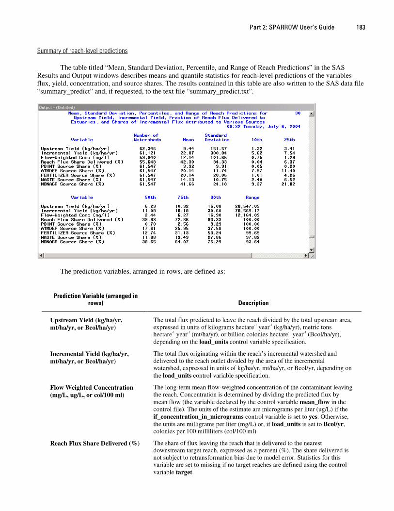
Part 2: SPARROW User’s Guide 183
Summary of reach-level predictions
The table titled “Mean, Standard Deviation, Percentile, and Range of Reach Predictions” in the SAS Results and Output windows describes means and quantile statistics for reach-level predictions of the variables flux, yield, concentration, and source shares. The results contained in this table are also written to the SAS data file “summary_predict” and, if requested, to the text file “summary_predict.txt”.
The prediction variables, arranged in rows, are defined as:
Prediction Variable (arranged in rows) Description
The total flux predicted to leave the reach divided by the total upstream area, expressed in units of kilograms hectare-1 year-1 (kg/ha/yr), metric tons hectare-1 year-1 (mt/ha/yr), or billion colonies hectare-1 year-1 (Bcol/ha/yr), depending on the load_units control variable specification.
Upstream Yield (kg/ha/yr, mt/ha/yr, or Bcol/ha/yr)
The total flux originating within the reach’s incremental watershed and delivered to the reach outlet divided by the area of the incremental watershed, expressed in units of kg/ha/yr, mt/ha/yr, or Bcol/yr, depending on the load_units control variable specification.
Incremental Yield (kg/ha/yr, mt/ha/yr, or Bcol/ha/yr)
The long-term mean flow-weighted concentration of the contaminant leaving the reach. Concentration is determined by dividing the predicted flux by mean flow (the variable declared by the control variable mean_flow in the control file). The units of the estimate are micrograms per liter (ug/L) if the if_concentration_in_micrograms control variable is set to yes. Otherwise, the units are milligrams per liter (mg/L) or, if load_units is set to Bcol/yr, colonies per 100 milliliters (col/100 ml)
Flow Weighted Concentration (mg/L, ug/L, or col/100 ml)
The share of flux leaving the reach that is delivered to the nearest downstream target reach, expressed as a percent (%). The share delivered is not subject to retransformation bias due to model error. Statistics for this variable are set to missing if no target reaches are defined using the control variable target.
Reach Flux Share Delivered (%)
The SPARROW Surface Water-Quality Model: Theory, Application and User Documentation 184
Description Prediction Variable (arranged in
rows)
[source_k] Source Share (%) The share of flux generated within the reach’s incremental watershed that can be attributed to the kth source in the model, expressed as a percent. [source_k] corresponds to the kth source listed in the srcvar control variable.
For each prediction variable, the columns contain the following descriptive statistics: the number of
reaches (incremental watersheds) summarized, the mean and standard deviation of the predictions across all reaches, the predictions corresponding to the 10th, 25th, 50th, 75th, and 90th percentile, and the range of the predictions.
Summaries are based on the prediction variables total_yield, inc_total_yield, concentration, map_del_frac, and sh_[source_k] included in the reach-level prediction output file “predict” (described in section 2.8.2.2, “Prediction output data files”). The total_yield, inc_total_yield, and concentration variables have been adjusted for retransformation bias due to model error but none of the variables have been adjusted for nonlinear prediction bias caused by sampling error in the coefficient estimates. See appendix D.6, “Prediction Output File ‘predict,’” for additional discussion of these variables, nonlinear prediction bias, and sampling error in coefficient estimates. Summary of reach-level predictions by land use (optional)
The table titled “Distribution of Yield Exported from SPARROW Watersheds” in the SAS Results and Output windows is produced only if the control variable if_distribute_yield_by_land_use is set to yes. The table shows summary statistics, across columns, of predicted yield for reaches grouped by predominant land use in the incremental watershed (land use classes are listed in rows). The results contained in the table are useful for comparing yield estimates obtained from SPARROW with estimates of yield by land use reported in the literature.
The columns of the table contain the following descriptive statistics for each land use classification: the number of reaches (incremental watersheds) that meet the classification criteria (as specified by the land_class_list control variable), the 10th, 25th, 50th, 75th, and 90th percentile incremental watershed yield for reaches classified into that land use, and the range of values for incremental watershed yield across all reaches classified into that land use, each expressed in units of kg/ha/yr, mt/ha/yr, or Bcol/ha/yr, depending on the specification of the control variable load_units,. Note that not all reaches are classified into a specified land use.
Summaries are based on the prediction variable inc_total_yield, which has been adjusted for retransformation bias associated with model error but has not been adjusted for bias arising from nonlinear sampling error in the coefficients (see appendix D.6, “Prediction Output File ‘predict,’” for additional discussion of inc_total_yield).
The results contained in this table are also written to the SAS data file “lu_yield_percentiles” and, if requested, to the text file “lu_yield_percentiles.txt”.
2.8.2.2 Prediction output data files
The SPARROW model writes to the directory “.\sparrow\results” several SAS data files (table 2.3) containing prediction results. In addition, if the control variable if_output_to_tab is set to yes, SPARROW also creates a duplicate tab-delimited text file for each of the SAS data files listed in table 2.3. Additional discussion of the general structure and function of each prediction output file is given in the following sections, and detailed descriptions of the variables in each file are included in appendix D, “Description of Output Files.”

Part 2: SPARROW User’s Guide 185
Table 2.3. Prediction output files (SAS data tables).
Output data file name Conditions for output Description of contents
predict Standard, if prediction is requested.
Contains predictions of total flux and flux by source for each reach in the stream network along with echo of user-selected input variables.
summary_ predict
Standard, if prediction is requested.
Contains a statistical summary of reach-level predictions.
lu_yield_ percentiles
Optional, if land-use summary is requested.
Contains a statistical summary of yield by land use.
test_predict, test_data
Optional, if prediction testing is requested.
Contains information to validate the detailed computations underlying the predictions for selected reaches.
Output file “predict” (standard, if prediction requested)
The file contains values for each reach of all the reach-level prediction variables. and also the reach identifiers and ancillary information as specified in the control variable optional_reach_information. The values of prediction variables are derived from the parametric coefficient estimates, and the variables include predicted total flux and flux by source, predicted flux (total and by source) without instream or reservoir attenuation, predicted incremental watershed flux (total and by source), the amount of flux removed in reservoirs, the fraction of flux leaving the reach delivered to a target reach, and the share of flux attributed to each source. If a bootstrap analysis is requested (as specified by the control variable n_boot_iter in the control file, see section 2.6.3.2, “Bootstrap iterations and seeds”), the file also includes a number of bootstrap-derived estimates to assess the errors inherent in most of the parametric predictions. The bootstrap assessment provides estimates of the bias and standard error of the parametric estimates, and derives confidence intervals for the predicted quantities. See appendix D.6, “Prediction Output File ‘predict,’” for detailed descriptions of each variable in this file. The tab-delimited version of this file is useful for transporting SPARROW results to ArcView for graphing reach-level results using a spatial coverage of the reach network.
Output file “summary_predict” (standard, if prediction requested)
The file contains a statistical summary of the reach-level prediction variables from the SAS data file “predict.” The file is organized with summary statistics serving as the column headings and the summarized prediction variables as the rows. The list of prediction variables included in the summary is given in section 2.8.2.1, “Summary results.” If bootstrapping is requested (the control variable n_boot_iter is set to a value greater than zero) and if the control variable if_print_boot_predictions is set to yes, the summaries are based on the prediction variables computed using the bootstrap estimates (variables with the mean_ prefix in the SAS data file “predict”), which include an adjustment for retransformation bias due to both model and sampling error. Otherwise the predictions are based on the parametric estimates (variables without the prefix mean_ in the SAS data file “predict”) with adjustment for retransformation bias caused by model error only.
The SPARROW Surface Water-Quality Model: Theory, Application and User Documentation 186
The summary statistics reported across the columns for each prediction variable are:
Description of summary statistics (columns) in the file “summary_predict”
n_watersheds - The number of watersheds or, equivalently, the number of reaches.
Mean - The mean across all reaches.
Std - The standard deviation across all reaches.
Range - The range of values across all reaches.
p_10 - The 10th percentile across all reaches.
p_25 - The 25th percentile
p_50 - The 50th percentile or median value.
p_75 - The 75th percentile.
p_90 - The 90th percentile.
Output file “lu_yield_percentiles” (optional)
File contains summary statistics of predicted incremental watershed yield for reaches grouped by predominant land use. Reaches are classified according to land use in the associated incremental watershed following the criteria defined in the control variable land_class_list. The file of summary statistics is created if the input SAS data file includes land-use variables, and if the control variable if_distribute_yield_by_land_use is set to yes. The columns of the file are the summary statistics and the rows are the land-use classes. The names of the land-use classes are taken from the names declared in the land_class_list control variable. The incremental watershed yield is the total flux originating from the reach’s incremental watershed and delivered to the reach outlet divided by incremental watershed area. All yield statistics are in units of kg/ha/yr, mt/ha/yr, or Bcol/ha/yr, depending on the specification of the load_units control variable.
Description of summary statistics (columns) in the file “lu_yield_percentiles”
inc_total_yield_n The number of incremental watersheds (reach segments) classified into the given land use.
inc_total_yield_range (kg/ha/yr, mt/ha/yr, or Bcol/ha/yr) The range of values for incremental watershed yield across all reaches classified into a given land use.
inc_total_yield_p10 (kg/ha/yr, mt/ha/yr, or Bcol/ha/yr) The 10th percentile incremental watershed yield for reaches classified into the given land use.
inc_total_yield_p25 (kg/ha/yr, mt/ha/yr, or Bcol/ha/yr) The 25th percentile incremental watershed yield for reaches classified into the given land use.
inc_total_yield_p50 (kg/ha/yr, mt/ha/yr, or Bcol/ha/yr) The 50th percentile, or median, incremental watershed yield for reaches classified into the given land use.
inc_total_yield_p75 (kg/ha/yr, mt/ha/yr, or Bcol/ha/yr) The 75th percentile incremental watershed yield for reaches classified into the given land use.
inc_total_yield_p90 (kg/ha/yr, mt/ha/yr, or Bcol/ha/yr) The 90th percentile incremental watershed yield for reaches classified into the given land use.

Part 2: SPARROW User’s Guide 187
2.8.3 Other file output SPARROW file output to the “.\sparrow\results” directory may also include the SAS file “comments_all”
containing comments generated by SPARROW during model execution, the SPARROW output in text file format, and intermediate results from bootstrap calculations.
2.8.3.1 Output file “comments_all”
File contains comments from model execution and is created only if comments from program execution are generated. The columns of the file are the iteration number (iter), the seed number (jter) and the descriptive comment (comment).
2.8.3.2 Text file output (optional)
If text format for output files is requested (control variable if_output_to_tab is set to yes), SPARROW also writes to the “.\sparrow\results” directory a duplicate tab-delimited text file for each SAS data file listed in tables 2.2 and 2.3. Note that because these files are in text format they are not included in the listing of files displayed in SAS Explorer. The text files can be easily imported into Arcview or a spreadsheet. The structure and variable names in the text files are the same as the structure and variable names in the equivalent SAS data files (see appendix D, “Description of Output Files”). The first row of each text file contains the list of variable names. When importing the text files into a spreadsheet, it will be necessary to designate as character variables certain variables that appear to be numeric. For example, the USGS station identification code is treated in SAS as a character variable because codes for eastern stations have a leading zero; without special intervention, the import of this variable into a spreadsheet is likely to result in a numeric field that has dropped the leading zero.
The following is a list of the tab-delimited files (duplicating SAS data files) written to the “.\sparrow\results” directory:
Estimation Output Files Prediction Output Files
summary_betaest.txt predict.txt
cov_betaest.txt summary_predict.txt
boot_betaest.txt (optional) LU_yield_percentiles.txt (optional)
resids.txt test_data.txt (optional)
test_resids.txt (optional) test_predict.txt (optional)
2.8.3.3 Bootstrap intermediate files (optional)
In the process of generating the bootstrap estimates, SPARROW writes a number of intermediate results to SAS data files in the “.\sparrow\results” directory. These files are automatically deleted upon completion of the bootstrap analysis. If a bootstrap analysis is terminated prior to completion (for example, execution interrupted by computer system shutdown), however, these files will appear in a listing of the “.\sparrow\results” directory, and must remain in that directory if the user intends to continue a previously initiated but uncompleted bootstrap analysis. These intermediate files include:
• a file named “predict_stats” containing reach running tallies for computing the bootstrap mean and variance for every prediction made by SPARROW, and
• a group of data files, each having the prefix “store_”, containing the prediction output from individual bootstrap iterations needed to compute the lower and upper bounds of the confidence interval for each prediction variable. A separate “store_” data file is created for each prediction variable generated by SPARROW.
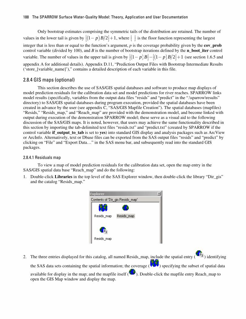
The SPARROW Surface Water-Quality Model: Theory, Application and User Documentation 188
Only bootstrap estimates comprising the symmetric tails of the distribution are retained. The number of
values in the lower tail is given by ( )1 2p B⎢ −⎣ 1⎥ +⎦ , where ⎢ ⎥⎣ ⎦ is the floor function representing the largest
integer that is less than or equal to the function’s argument, p is the coverage probability given by the cov_prob control variable (divided by 100), and B is the number of bootstrap iterations defined by the n_boot_iter control
variable. The number of values in the upper tail is given by ( ) ( )1 1 2p B p B 1⎢ ⎥ ⎢ ⎥− − − +⎣ ⎦ ⎣ ⎦ (see section 1.6.5 and
appendix A for additional details). Appendix D.11, “Prediction Output Files with Bootstrap Intermediate Results (‘store_[variable_name]’),” contains a detailed description of each variable in this file.
2.8.4 GIS maps (optional) This section describes the use of SAS/GIS spatial databases and software to produce map displays of
model prediction residuals for the calibration data set and model predictions for river reaches. SPARROW links model results (specifically, variables from the output data files “resids” and “predict” in the “.\sparrow\results” directory) to SAS/GIS spatial databases during program execution, provided the spatial databases have been created in advance by the user (see appendix C, “SAS/GIS Mapfile Creation”). The spatial databases (mapfiles) “Resids,” “Resids_map,” and “Reach_map” are provided with the demonstration model, and become linked with output during execution of the demonstration SPARROW model; these serve as a visual aid to the following discussion of the SAS/GIS maps. It is noted, however, that users may achieve the same functionality described in this section by importing the tab-delimited text files “resids.txt” and “predict.txt” (created by SPARROW if the control variable if_output_to_tab is set to yes) into standard GIS display and analysis packages such as ArcView or ArcInfo. Alternatively, text or Dbase files can be exported from the SAS output files “resids” and “predict” by clicking on “File” and “Export Data…” in the SAS menu bar, and subsequently read into the standard GIS packages.
2.8.4.1 Residuals map
To view a map of model prediction residuals for the calibration data set, open the map entry in the SAS/GIS spatial data base “Reach_map” and do the following:
1. Double-click Libraries in the top level of the SAS Explorer window, then double-click the library “Dir_gis” and the catalog “Resids_map.”
2. The three entries displayed for this catalog, all named Resids_map, include the spatial entry ( ) identifying
the SAS data sets containing the spatial information; the coverage ( ) specifying the subset of spatial data
available for display in the map; and the mapfile itself ( ). Double-click the mapfile entry Reach_map to open the GIS Map window and display the map.
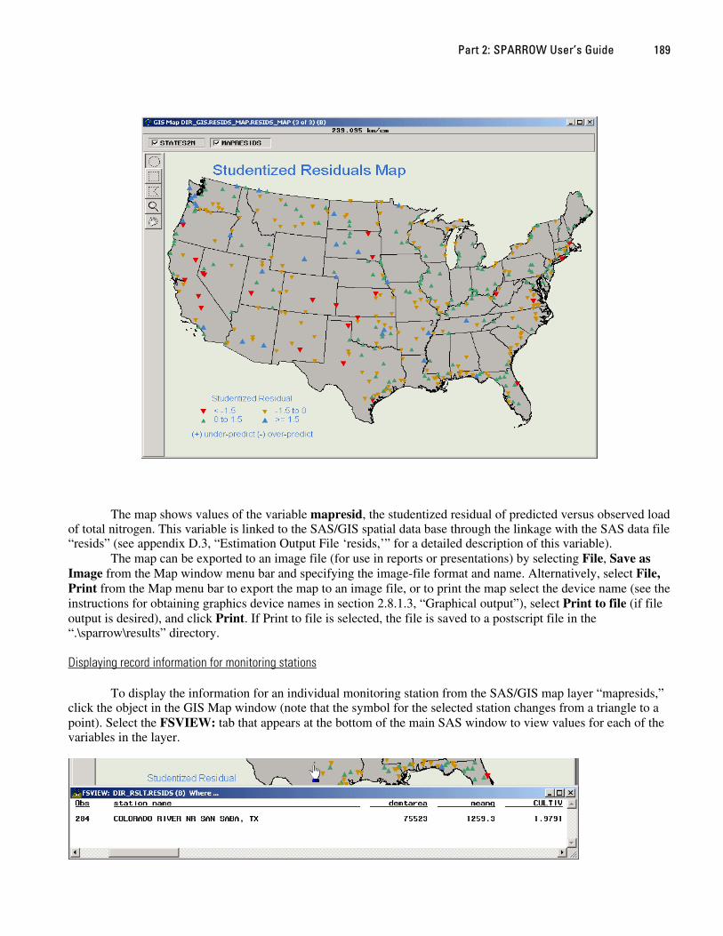
Part 2: SPARROW User’s Guide 189
The map shows values of the variable mapresid, the studentized residual of predicted versus observed load of total nitrogen. This variable is linked to the SAS/GIS spatial data base through the linkage with the SAS data file “resids” (see appendix D.3, “Estimation Output File ‘resids,’” for a detailed description of this variable).
The map can be exported to an image file (for use in reports or presentations) by selecting File, Save as Image from the Map window menu bar and specifying the image-file format and name. Alternatively, select File, Print from the Map menu bar to export the map to an image file, or to print the map select the device name (see the instructions for obtaining graphics device names in section 2.8.1.3, “Graphical output”), select Print to file (if file output is desired), and click Print. If Print to file is selected, the file is saved to a postscript file in the “.\sparrow\results” directory.
Displaying record information for monitoring stations
To display the information for an individual monitoring station from the SAS/GIS map layer “mapresids,” click the object in the GIS Map window (note that the symbol for the selected station changes from a triangle to a point). Select the FSVIEW: tab that appears at the bottom of the main SAS window to view values for each of the variables in the layer.
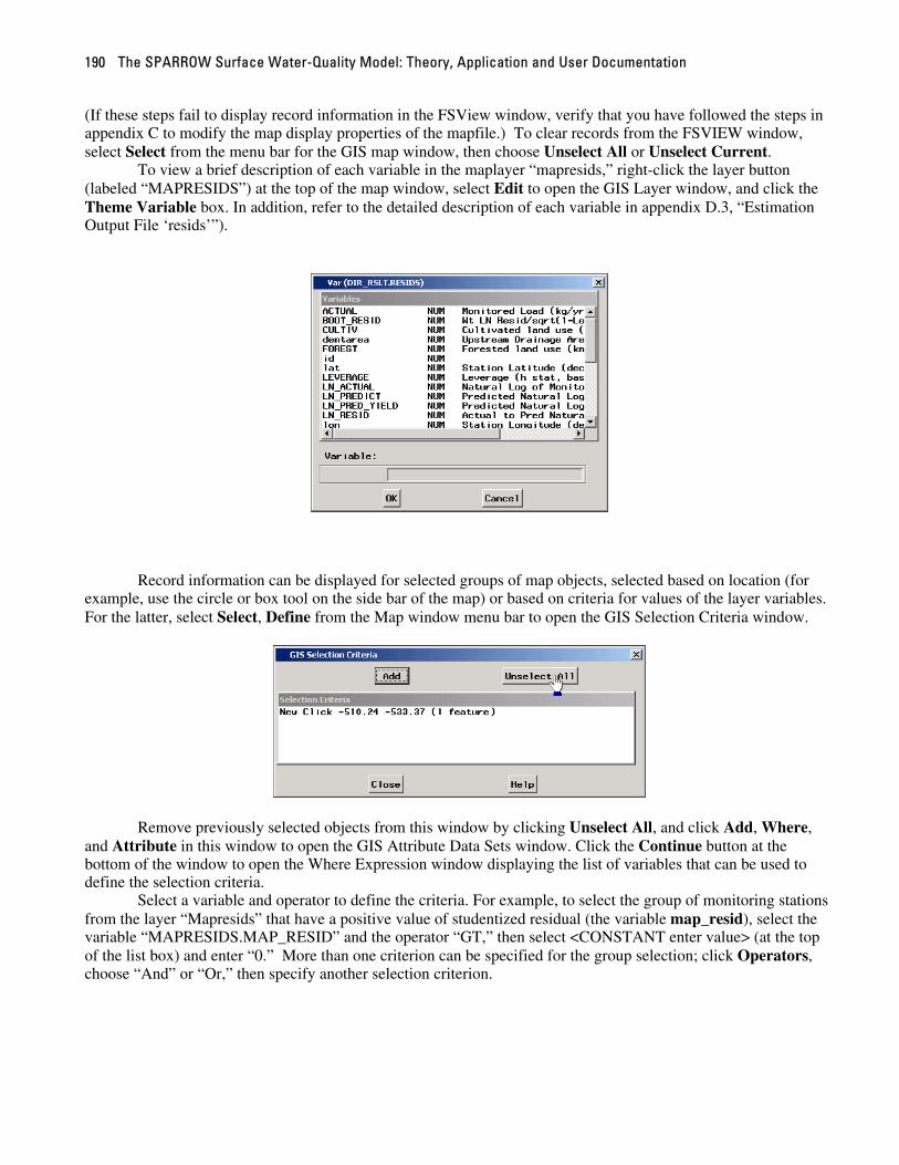
The SPARROW Surface Water-Quality Model: Theory, Application and User Documentation 190
(If these steps fail to display record information in the FSView window, verify that you have followed the steps in appendix C to modify the map display properties of the mapfile.) To clear records from the FSVIEW window, select Select from the menu bar for the GIS map window, then choose Unselect All or Unselect Current.
To view a brief description of each variable in the maplayer “mapresids,” right-click the layer button (labeled “MAPRESIDS”) at the top of the map window, select Edit to open the GIS Layer window, and click the Theme Variable box. In addition, refer to the detailed description of each variable in appendix D.3, “Estimation Output File ‘resids’”).
Record information can be displayed for selected groups of map objects, selected based on location (for example, use the circle or box tool on the side bar of the map) or based on criteria for values of the layer variables. For the latter, select Select, Define from the Map window menu bar to open the GIS Selection Criteria window.
Remove previously selected objects from this window by clicking Unselect All, and click Add, Where, and Attribute in this window to open the GIS Attribute Data Sets window. Click the Continue button at the bottom of the window to open the Where Expression window displaying the list of variables that can be used to define the selection criteria.
Select a variable and operator to define the criteria. For example, to select the group of monitoring stations from the layer “Mapresids” that have a positive value of studentized residual (the variable map_resid), select the variable “MAPRESIDS.MAP_RESID” and the operator “GT,” then select <CONSTANT enter value> (at the top of the list box) and enter “0.” More than one criterion can be specified for the group selection; click Operators, choose “And” or “Or,” then specify another selection criterion.

Part 2: SPARROW User’s Guide 191
Click OK to accept the selection. Records for the group of objects will be displayed in the FSVIEW table window. The selected monitoring stations are shown on the residuals map as small cyan dots (the first station on the FSVIEW table list appears as a small red dot on the map).
2.8.4.2 Reach map
To view the map of predicted flux for each stream reach, return to the “Dir_gis” library level in the SAS
Explorer window, double-click the catalog “Reach_map” and then the map entry ( ) for “Reach_map.”
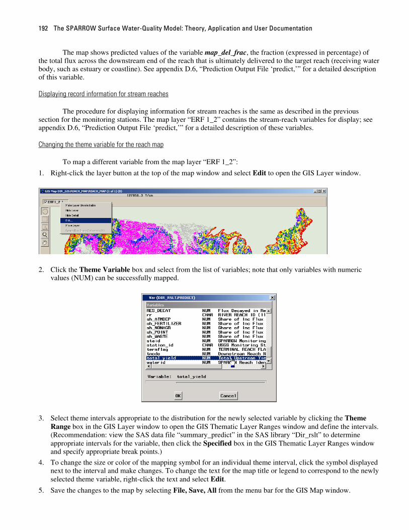
The SPARROW Surface Water-Quality Model: Theory, Application and User Documentation 192
The map shows predicted values of the variable map_del_frac, the fraction (expressed in percentage) of the total flux across the downstream end of the reach that is ultimately delivered to the target reach (receiving water body, such as estuary or coastline). See appendix D.6, “Prediction Output File ‘predict,’” for a detailed description of this variable.
Displaying record information for stream reaches
The procedure for displaying information for stream reaches is the same as described in the previous section for the monitoring stations. The map layer “ERF 1_2” contains the stream-reach variables for display; see appendix D.6, “Prediction Output File ‘predict,’” for a detailed description of these variables.
Changing the theme variable for the reach map
To map a different variable from the map layer “ERF 1_2”:
1. Right-click the layer button at the top of the map window and select Edit to open the GIS Layer window.
2. Click the Theme Variable box and select from the list of variables; note that only variables with numeric values (NUM) can be successfully mapped.
3. Select theme intervals appropriate to the distribution for the newly selected variable by clicking the Theme Range box in the GIS Layer window to open the GIS Thematic Layer Ranges window and define the intervals. (Recommendation: view the SAS data file “summary_predict” in the SAS library “Dir_rslt” to determine appropriate intervals for the variable, then click the Specified box in the GIS Thematic Layer Ranges window and specify appropriate break points.)
4. To change the size or color of the mapping symbol for an individual theme interval, click the symbol displayed next to the interval and make changes. To change the text for the map title or legend to correspond to the newly selected theme variable, right-click the text and select Edit.
5. Save the changes to the map by selecting File, Save, All from the menu bar for the GIS Map window.
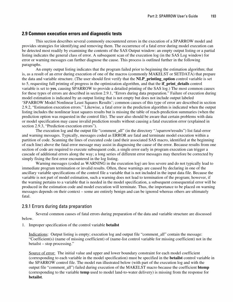
Part 2: SPARROW User’s Guide 193
2.9 Common execution errors and diagnostic tests This section describes several commonly encountered errors in the execution of a SPARROW model and
provides strategies for identifying and removing them. The occurrence of a fatal error during model execution can be detected most readily by examining the contents of the SAS Output window: an empty output listing or a partial listing indicates the general class of error. A subsequent scan of the execution log (in the SAS Log window) for error or warning messages can further diagnose the cause. This process is outlined further in the following paragraphs.
An empty output listing indicates that the program failed prior to beginning the estimation algorithm; that is, as a result of an error during execution of one of the macros (commonly MAKELST or SETDATA) that prepare the data and variable structure. (The user should first verify that the NLP_printing_option control variable is set to 5, requesting full printing of progress in the optimization algorithm, and that the if_print_details control variable is set to yes, causing SPARROW to provide a detailed printing of the SAS log.) The most common causes for these types of errors are described in section 2.9.1, “Errors during data preparation.” Failure of execution during model estimation is indicated by an output listing that is not empty but does not include output labeled ‘SPARROW Model Nonlinear Least Squares Results’; common causes of this type of error are described in section 2.9.2, “Estimation execution errors.” Likewise, a fatal error in the prediction algorithm is indicated when the output listing includes the nonlinear least squares results but is missing the table of reach-prediction summaries (when the prediction option was requested in the control file). The user also should be aware that certain problems with data or model specification may cause invalid prediction results without causing a fatal execution error (explained in section 2.9.3, “Prediction execution errors”).
The execution log and the output file “comment_all” (in the directory “.\sparrow\results”) list fatal-error and warning messages. Typically, messages coded as ERROR are fatal and terminate model execution within a partition of code. Scanning the lines of executed code (and their associated SAS macro, identified at the beginning of each line) above the fatal error message may assist in diagnosing the cause of the error. Because results from one section of code are required to execute subsequent code, a single error early in program execution can trigger a cascade of additional errors along the way; a long series of different error messages may therefore be corrected by simply fixing the first error encountered in the log listing.
Warning messages (coded as WARNING in the execution log) are less severe and do not typically lead to immediate program termination or invalid results. Often, these warnings are caused by declaring in one of the ancillary variable specifications of the control file a variable that is not included in the input data file. Because the variable is not part of model estimation, such a warning does not lead to termination of the program; however, if the warning pertains to a variable that is needed in the model specification, a subsequent consequential error will be produced in the estimation code and model execution will terminate. Thus, the importance to be placed on warning messages depends on their context – some are entirely benign and can be ignored whereas others are ultimately fatal.
2.9.1 Errors during data preparation
Several common causes of fatal errors during preparation of the data and variable structure are discussed below.
1. Improper specification of the control variable betailst Indications: Output listing is empty; execution log and output file “comment_all” contain the message: “Coefficient(s) (name of missing coefficient) of (name-list control variable for missing coefficient) not in the betailst – stop processing.” Source of error: The initial value and upper and lower boundary constraint for each model coefficient (corresponding to each variable in the model specification) must be specified in the betailst control variable in the SPARROW control file. The model run illustrated below (with part of the execution log and with the output file “comment_all”) failed during execution of the MAKELST macro because the coefficient btemp (corresponding to the variable temp used to model land-to-water delivery) is missing from the response for betailst.

The SPARROW Surface Water-Quality Model: Theory, Application and User Documentation 194
Solution: Find and edit in the SPARROW control file the response for the control variable betailst, adding the name, initial values, and upper and lower boundary constraints for the missing coefficient.
2. Improper specification of name lists for variables or coefficients Indications: Output listing is blank; execution log and output file “comment_all” contain the message: “Number of delivery variables (x) and delivery variable coefficients (y) are unequal – stop processing.” Source of error: When a variable is added (or dropped) as a predictor in the model, changes must be made to the responses for two separate control variables in the SPARROW control file: the response for one of the variable name lists (srcvar, delvar, or decvar), and for the associated coefficient name list (bsrcvar, bdelvar, or bdecvar). The model run illustrated below (with part of the execution log and with the output file “comment_all”) failed during the execution of the MAKELST macro because the coefficient btemp (associated with the variable temp used to model land-to-water delivery) was included in the coefficient name list bdlvvar, but the associated delivery variable temp was missing from the name list dlvvar.
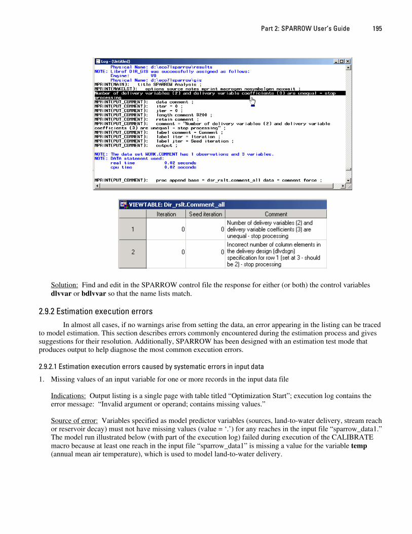
Part 2: SPARROW User’s Guide 195
Solution: Find and edit in the SPARROW control file the response for either (or both) the control variables dlvvar or bdlvvar so that the name lists match.
2.9.2 Estimation execution errors
In almost all cases, if no warnings arise from setting the data, an error appearing in the listing can be traced to model estimation. This section describes errors commonly encountered during the estimation process and gives suggestions for their resolution. Additionally, SPARROW has been designed with an estimation test mode that produces output to help diagnose the most common execution errors.
2.9.2.1 Estimation execution errors caused by systematic errors in input data
1. Missing values of an input variable for one or more records in the input data file Indications: Output listing is a single page with table titled “Optimization Start”; execution log contains the error message: “Invalid argument or operand; contains missing values.” Source of error: Variables specified as model predictor variables (sources, land-to-water delivery, stream reach or reservoir decay) must not have missing values (value = ‘.’) for any reaches in the input file “sparrow_data1.” The model run illustrated below (with part of the execution log) failed during execution of the CALIBRATE macro because at least one reach in the input file “sparrow_data1” is missing a value for the variable temp (annual mean air temperature), which is used to model land-to-water delivery.
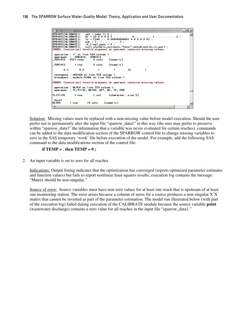
The SPARROW Surface Water-Quality Model: Theory, Application and User Documentation 196
Solution: Missing values must be replaced with a non-missing value before model execution. Should the user prefer not to permanently alter the input file “sparrow_data1” in this way (the user may prefer to preserve within “sparrow_data1” the information that a variable was never evaluated for certain reaches), commands can be added to the data modification section of the SPARROW control file to change missing variables to zero in the SAS temporary ‘work’ file before execution of the model. For example, add the following SAS command to the data modifications section of the control file:
if TEMP = . then TEMP = 0 ;
2. An input variable is set to zero for all reaches Indications: Output listing indicates that the optimization has converged (reports optimized parameter estimates and function values) but fails to report nonlinear least squares results; execution log contains the message: “Matrix should be non-singular.” Source of error: Source variables must have non-zero values for at least one reach that is upstream of at least one monitoring station. The error arises because a column of zeros for a source produces a non-singular X’X matrix that cannot be inverted as part of the parameter estimation. The model run illustrated below (with part of the execution log) failed during execution of the CALIBRATE module because the source variable point (wastewater discharge) contains a zero value for all reaches in the input file “sparrow_data1.”
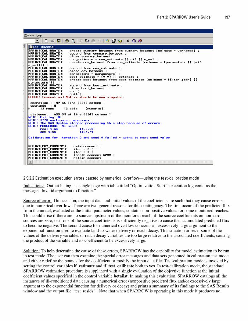
Part 2: SPARROW User’s Guide 197
2.9.2.2 Estimation execution errors caused by numerical overflow—using the test-calibration mode
Indications: Output listing is a single page with table titled “Optimization Start;” execution log contains the message “Invalid argument to function.” Source of error: On occasion, the input data and initial values of the coefficients are such that they cause errors due to numerical overflow. There are two general reasons for this contingency. The first occurs if the predicted flux from the model, evaluated at the initial parameter values, contains non-positive values for some monitored reaches. This could arise if there are no sources upstream of the monitored reach, if the source coefficients on non-zero sources are zero, or if one of the source coefficients is sufficiently negative to cause the accumulated predicted flux to become negative. The second cause for numerical overflow concerns an excessively large argument to the exponential function used to evaluate land-to-water delivery or reach decay. This situation arises if some of the values of the delivery variables or reach decay variables are too large relative to the associated coefficients, causing the product of the variable and its coefficient to be excessively large.
Solution: To help determine the cause of these errors, SPARROW has the capability for model estimation to be run in test mode. The user can then examine the special error messages and data sets generated in calibration test mode and either redefine the bounds for the coefficient or modify the input data file. Test-calibration mode is invoked by setting the control variables if_estimate and if_test_calibrate both to yes. In test-calibration mode, the standard SPARROW estimation procedure is supplanted with a single evaluation of the objective function at the initial coefficient values specified in the control variable betailst. In making this evaluation, SPARROW catalogs all the instances of ill-conditioned data causing a numerical error (nonpositive predicted flux and/or excessively large argument to the exponential function for delivery or decay) and prints a summary of its findings to the SAS Results window and the output file “test_resids.” Note that when SPARROW is operating in this mode it produces no
The SPARROW Surface Water-Quality Model: Theory, Application and User Documentation 198
output except for the error messages and special test data sets; test-calibration mode should be invoked therefore only when a problem has been encountered. Nonpositive predicted flux
If the predicted flux for a monitoring station is nonpositive, SPARROW (running in test-calibration mode) prints the following message to the SAS Results window:
Non-positive rchld <rchld value> for obs: <observation number> station: <[staid] value> at reach ID:
<[waterid] value>,
where <rchld value> is the negative estimate of predicted flux, <observation number> is the sequential observation number in the input file “sparrow_data1” corresponding to the given monitored reach, <[staid] value> is the station identifier given by the variable identified by the control variable staid, and <[waterid] value> is the reach identifier given by the variable identified by the control variable waterid. A close examination of the input data for reaches upstream of a negative flux estimate will usually determine the underlying cause. In most cases, the problem can be corrected by specifying appropriate bounds on the coefficients in the betailst control variable. Argument to delivery or decay function exceeds maximum
SPARROW scans the input data file to determine if there are instances in which the absolute value of the product of a land-to-water delivery variable (identified by the control variable dlvvar) and its associated coefficient (control variable bdlvvar) or a reach decay variable (identified by the control variable decvar) and its associated coefficient (identified by the control variable bdecvar) exceeds 709—the maximum value the exponential function can numerically evaluate. If any cases of large products are detected, SPARROW prints a report to the SAS Results window consisting of the number of reaches with excessive products, the values of the delivery coefficients, and the reach identifier (waterid) and values of the delivery variables for the first few exceeding reaches (up to five). A similar report is printed if there are any excessively large products of a reach decay variable and its associated coefficient.
Although the solution for excessively large products of reach decay or land-to-water delivery variables and their associated coefficients may be as simple as appropriately bounding the relevant coefficients, more often the root cause of the problem is that one of the delivery or decay variables has an extremely large range. In this case, the appropriate correction involves redefining the ill-conditioned variable; a logarithm transformation of the offending variable may solve the problem.
2.9.2.3 Estimation execution errors related to bootstrap analysis
For applications using bootstrapping, messages are printed to the SAS Log window documenting the completion of bootstrap resampling iterations. If errors are encountered only for specific bootstrap iterations, the execution log provides sufficient information to determine which iterations are affected. SPARROW can be run for these specific iterations using the start_iter, start_jter and n_boot_iter control variables to try and isolate the cause of the problem. Note, however, that if the SPARROW model cannot be estimated for a particular bootstrap iteration, SPARROW automatically skips the random seed value that gives rise to the estimation problem and goes on to the next seed value. In this case, the jter counter will increment by one and the iter counter will remain unchanged.
Part 2: SPARROW User’s Guide 199
2.9.3 Prediction execution errors
SPARROW must make predictions as part of the estimation process. If the model is successfully estimated, then typically it is also free of fatal errors during the prediction algorithm. Prediction output from a model that is executed without fatal errors is not necessarily valid, however (for example, if a process specification is coded incorrectly), and the user should evaluate validity using the lines of evidence described in this section.
2.9.3.1 Test-prediction mode
SPARROW can be run in a test-prediction mode to produce two test files, “test_predict” and “test_data” (contained in the directory “.\sparrow\results”) that enable the user to check the intermediate calculations leading to the final prediction results. Test-prediction mode is invoked by setting the control variable if_test_predict to yes. A detailed description of each test file is included in appendices D.9 and D.10, “Prediction Output File ‘test_data’” and “Prediction Output File ‘test_predict.’”
The following are examples of potential problems that can be detected and resolved by inspection of output files produced from the test-predict mode. To assist in checking prediction output, it is helpful to load text file versions of SPARROW output into a spreadsheet. Text file output is obtained by setting the control variable if_output_to_tab to yes in the control file.
1. Integrity of the accumulation process
The integrity of the accumulation process is one potential concern that can be thoroughly examined with the test output. Included in the “test_data” output file are estimates of flux at the upstream node of the test reach, the incremental flux generated in the test reach, and the reach and reservoir delivery factors associated with the test reach. The flux estimate for the test reach can be independently verified by loading the text file version of the “test_data” data file into a spreadsheet and undertaking a series of calculations on the included variables. The accumulation process is valid if the estimate of flux for the reach, as given by the variable PLOAD_TOTAL in the “test_predict” data file, equals the product of the upstream node flux (NODE_TOTAL), the fraction diverted value ([frac]), and the values of the reach and reservoir delivery factors (RCHDCAYF and RESDCAYF), plus the estimate of incremental flux delivered to the reach outlet (INCDDSRC_TOTAL). The value of the incremental flux delivered to the reach can itself be checked by comparing the value of INCDDSRC_TOTAL given in the “test_data” file with the product of RESDCAYF, the square root of RCHDCAYF and the incremental flux estimate given by the variable PLOAD_INC_TOTAL in the file “test_predict.”
An additional validation of the accumulation process is possible by comparing prediction output from the “predict” file with output from the “test_data” file. To perform the check, open the “predict” and “test_data” SAS files in the SAS Viewtable utility. From the “test_data” output, determine the value of the “from node” variable for the test reach. Then select the reaches in the “predict” data set that flow into the test reach by clicking on Data/Where in the command menu and doing a selection of all reaches that have values for the “to node” equal to the value of “from node” for the test reach. The accumulation process is valid if the upstream node estimate of flux given by the variable NODE_TOTAL in the “test_data” file, times MEAN_EXP_WEIGHTED_ERROR in the “summary_betaest” file, equals the sum of the PLOAD_TOTAL variable for the selected upstream reaches in the “predict” file.
2. Integrity of the reach and reservoir delivery processes
An independent check on the reach and reservoir delivery processes can be made by loading the text file version of the “test_data” and “summary_betaest” files into a spreadsheet and applying the process equations as defined in the control variables reach_decay_specification and reservoir_decay_specification specified in the control file. The processes are validated if the spreadsheet estimates match the estimates for RCHDCAYF and RESDCAYF given in the “test_data” file.
3. Integrity of the land-to-water delivery process
The land-to-water delivery process can be checked for individual sources by loading text file versions of the “test_data” and “summary_betaest” output files into a spreadsheet. To test the delivery process, the variable
The SPARROW Surface Water-Quality Model: Theory, Application and User Documentation 200
INCDDSRC_[source_k] (for source k) is first divided by the product of the source-k source coefficient ([bsrcvar_k]), the source-k source ([srcvar_k]), the reservoir delivery factor (RESDCAYF), and the square root of the reach delivery factor (the square root of RCHDCAYF). The resulting value is then compared to the factor computed from the specified land-to-water-delivery function, defined by the control variable incr_delivery_specification, applied to the pertinent land-to-water delivery variables and coefficients. In computing the factor, it is necessary to include only those land-to-water delivery variables that pertain to source k, as defined in the control file by the dlvdsgn matrix.
4. Integrity of the bootstrap estimates
The “test_predict” output data set includes bootstrap iteration intermediate results that permit the checking of bootstrap estimates of bias adjustment, standard error, and confidence interval bounds. To perform the checks, the text file version of the “test_predict” output file can be loaded into a spreadsheet and the equations from sections 1.6.3-1.6.5 of Part 1 can be applied to the bootstrap iteration values of PLOAD_PREDICT to obtain independent estimates of the bootstrap summary statistics MN_PLOAD_PREDICT, SD_PLOAD_PREDICT, and CI_LOW_PLOAD_TOTAL and CI_HI_PLOAD_TOTAL.
2.9.3.2 Evaluation of summary table of reach predictions
In addition to the test files generated by the test-prediction mode, certain characteristics of the reach-prediction table potentially indicate invalid prediction results. 1. Inappropriate accumulation of flux along the stream reach network
Indication: The maximum predicted value (reported as ‘Range’ in the summary table of reach predictions) for “ Reach Flux Share Delivered” exceeds 100 percent. (The summary table titled “Mean, Standard Deviation, Percentiles, and Range of Reach Predictions” is included in the output listing and also in the output SAS data file “Summary_predict”). Source of error: This may result from duplicate reaches in the input file “sparrow_data1,” which causes the reach shares to be duplicated, or may arise in a model in which the stream channel represents a source of flux. For the model run illustrated below, the input data file contained duplicate records with the same value for the variable waterid, and the problem was resolved by removing duplicate reach records from the input file “sparrow_data1.”
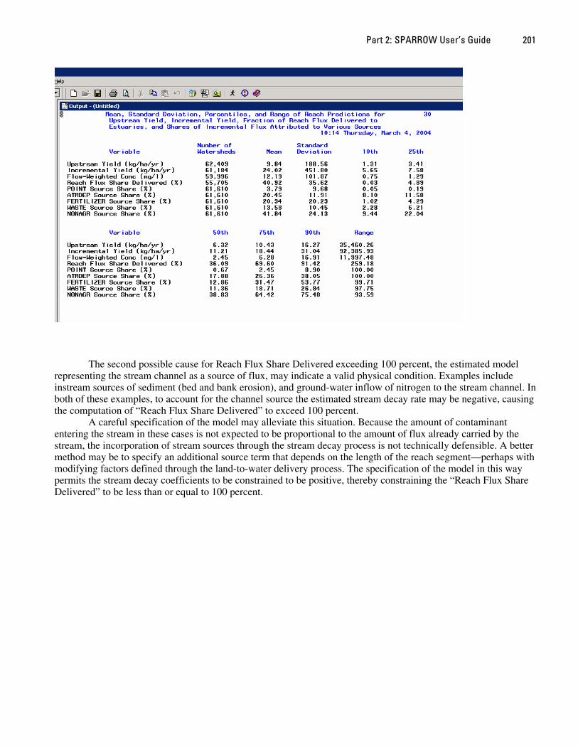
Part 2: SPARROW User’s Guide 201
The second possible cause for Reach Flux Share Delivered exceeding 100 percent, the estimated model representing the stream channel as a source of flux, may indicate a valid physical condition. Examples include instream sources of sediment (bed and bank erosion), and ground-water inflow of nitrogen to the stream channel. In both of these examples, to account for the channel source the estimated stream decay rate may be negative, causing the computation of “Reach Flux Share Delivered” to exceed 100 percent.
A careful specification of the model may alleviate this situation. Because the amount of contaminant entering the stream in these cases is not expected to be proportional to the amount of flux already carried by the stream, the incorporation of stream sources through the stream decay process is not technically defensible. A better method may be to specify an additional source term that depends on the length of the reach segment—perhaps with modifying factors defined through the land-to-water delivery process. The specification of the model in this way permits the stream decay coefficients to be constrained to be positive, thereby constraining the “Reach Flux Share Delivered” to be less than or equal to 100 percent.
The SPARROW Surface Water-Quality Model: Theory, Application and User Documentation 202
2.10 References Alexander, R.B., Smith, R.A., and Schwarz, G.E., 2000, Effect of stream channel size on the delivery of nitrogen to
the Gulf of Mexico: Nature, v. 403, p. 758-761. Smith, R.A., Schwarz, G.E., and Alexander, R.B., 1997, Regional interpretation of water-quality monitoring data:
Water Resources Research, v. 33, p. 2781-2798. Statistical Analysis Systems Institute, 2000a, SAS language reference – dictionary, version 8: Cary, NC, SAS
Institute, Inc., 500 p. Statistical Analysis Systems Institute, 2000b, SAS/IML user’s guide, version 8: Cary, NC, SAS Institute, Inc. Statistical Analysis Systems Institute, 2000c, SAS/Insight user’s guide, version 8: Cary, NC, SAS Institute, Inc. Wolock, D.M., 1993, Simulating the variable-source-area concept of streamflow generation with the watershed
model TOPMODEL, U.S. Geological Survey Water-Resources Investigations Report 93-4124, 33 p.