Parochial Politics: Ethnic Preferences and Politician Corruption

Abhijit V. Banerjee and Rohini Pande∗

Abstract

Does political competition along ethnic lines worsen politician quality? We show that, in

a world with incomplete policy commitment, a greater tendency to vote along ethnic lines

reduces politician quality even when it does not affect the availability of good candidates and

there are no systematic differences in candidate quality across parties. Specifically, ethnic

party competition lowers the average winner quality for the pro-majority party. The opposite

holds for minority party winners. Overall, relative to losers, the average winner quality in a

jurisdiction falls. Empirical evidence based on data from a survey on politician corruption

that we recently conducted in North India is remarkably consistent with the predictions of

the theory.

1 Introduction

Our vote and your rule, this will not work anymore

Campaign slogan of BSP, an Indian low caste party1

One of the most influential hypotheses in political economy is that societies which are polarized

along ethnic, religious or linguistic lines produce poor economic outcomes. While papers differ

in how they measure polarization, under most metrics an increase in the relative importance

of ethnic identity in shaping preferences increases polarization. Recent empirical contributions

suggest that increased polarization is correlated with reduced GDP (Alesina, Baqir, and Easterly

1999), lower GDP growth (Easterly and Levine 1997), worse private provision of public goods

(Miguel and Gugerty (2004), Khwaja (2004)) and increased corruption (Mauro 1995).∗The authors are from MIT and Harvard respectively. We are grateful to Rasika Duggal and, especially,

Santosh Kumar and Bhartendu Trivedi for organizing the survey. Pande thanks NSF for financial support forthis project under grant SES-0417634

1The original slogan in Hindi reads ‘Mat hamara raj tumhara nahin chalega

1

Why should polarization worsen economic outcomes? There is some suggestive evidence that

an important reason is worse collective action. Polarization lowers participation in collective

activities (Alesina and Ferrara 2000), creates dispersed living arrangements (Alesina, Baqir,

and Hoxby 2004), reduces the effectiveness of social sanctions (Miguel and Gugerty 2004) and

increases the likelihood of civil conflict (Montalvo and Querol 2005).

In this paper we explore a very simple, closely related but distinct, channel which is especially

relevant in societies that rely on electoral competition to get effective leadership. Our starting

point is that voters share a common interest in something we call politician quality, but differ in

their parochial preferences, which involves favoring politicians or parties that share their ethnic

or religious background.2

If politics played out as in the standard, Downsian, model, where parties care about winning

and can commit to implementing specific policies, then parochialism may not create much of

a problem: the electoral incentives of a party or politician are always to promise high quality.

This is no longer true if, as in the so-called citizen candidate models, parties cannot commit to

specific policies. Then a party with the right ethnic markers might get chosen, even if the policies

that it would implement if elected are of relatively low quality. Put differently, in this class of

models the policy is a characteristic of the party or the candidate and cannot be separated from

their ethnic attributes. Obviously the stronger the ethnic preferences the bigger the shortfall in

quality that would be tolerated by voters.

This is the basic idea that is developed in this paper. We build a simple model where voters care

about candidate quality and ethnicity. Two parties compete by picking the most marketable

candidates from party-specific lists of potential candidates. Candidates differ in quality and in

the strength of their association with the majority group. This model has the (not surprising)

testable implication that increased polarization, as defined by a strengthening of ethnic pref-

erences, lowers the quality of elected politicians belonging to the party which represents the

population majority group in that area. The opposite holds for politicians from the minor-

ity party. Within a jurisdiction, under relatively general assumptions, polarization lowers the

average quality of winners (relative to losers).

An alternative, but closely related, model is one where parties have policy preferences. With2Horowitz (1985), the classic book on ethnic conflict and politics, defines ethnic parties as those which derive

their support from an identifiable ethnic group and serves the interests of that group.

2

aggregate uncertainty about voter behavior (as, for instance, in a probabilistic voting model)

a party with policy preferences might accept a lower probability of winning in order to ensure

that, conditional on winning, the policy that it particularly favors gets implemented. Thus a

party that favors a certain ethnic group, might sacrifice some quality and hence run the risk of

losing, in order to ensure that a candidate from that group gets chosen. The more polarized

the population, the less risky it is for the majority party to field its favored candidate/policy

instead of the highest quality candidate.3

Ethnic political parties are an important part of the political landscape in many democracies,

and many argue ethnic party competition is particularly relevant in ethnically diverse low income

countries (see, for instanceChua (2003), Posner (2005) (on Africa) and Chandra (2004) (on South

Asia )). Ethnic parties are rarer in more homogenous Western countries, but Belgium, and to a

less extent Spain, Ireland and Canada, provide notable exceptions.

Our empirical analysis in this paper focusses on Northern India, which saw a significant rise

in ethnic party competition since the mid 1980s. We examine two data-sets relating to Uttar

Pradesh (UP) – India’s most populous state and a state which has, in recent years, seen a

significant rise in both ethnic politics and political corruption.4 We examine data on the criminal

records of national legislators from Uttar Pradesh on the eve of their election to the legislature

in 2004, and panel data on politician corruption from a survey which we conducted. The survey

collected information on politicians in over a hundred legislative jurisdictions who stood for

election in 1969, 1980 and 1996.

We use these data to corroborate our theoretical claims. With the cross-sectional national

legislator data we exploit geographic variation in jurisdiction bias, as measured by the population

share of low castes, for identification. A winner from a jurisdiction biased in favor of the party

(i.e. where the party is pro-majority in its ethnic affiliation) is more likely to have a criminal3Our model of politician selection is related to Myerson (1993) and Glaeser, Ponzetto, and Shapiro (2005).

Myerson (1993) shows that, with strategic voting and multi-dimensional preferences, plurality rule systems aresensitive to a coordination failure wherein voters vote for low quality candidates since they fear that switchingtheir vote may cause their least preferred candidate to win. Our focusing on two party competition implies that,like Glaeser, Ponzetto, and Shapiro (2005), we abstract from strategic voting issues.Glaeser, Ponzetto, and Shapiro(2005) examine strategic policy extremism by the two major US parties. While they consider multi-dimensionalpolicy-making they assume throughout that the two dimensions are independent. In contrast, we consider bundledpreferences across the two dimensions.

4“As a state of the Indian union, its dirty, bitter, caste-based and often violent politics still make waves thatspread beyond its borders. Uttar Pradesh is a particularly acute example of the increasing criminal involvementin Indian politics.”the Economist, May 2003

3

record relative to the winner from the same party in a less biased jurisdiction.

These results, while strongly suggestive of the idea that polarization affects politician quality,

remain subject to the usual concerns facing cross-sectional comparisons. For this reason we

use our survey data to examine how increased voter polarization over time within the same

jurisdiction alters politician quality. Here, we combine cross-jurisdiction variation in bias with

time-series variation in the importance of ethnic politics for identification. The upsurge in ethnic

party politics since early 1980s is often described as a ‘second democratic upsurge’ Yadav (2000)

and was driven by increased caste consciousness and political activism among the historically

disadvantaged lower caste groups. Figures 1 and 2 demonstrate the dramatic rise in the vote

share of low caste parties and presence of low caste legislators since the mid-1980s in UP. In

Table 1 we see that by 1996, voting patterns exhibited substantial ethnic identification: in 1996,

both high and low caste voters were significantly more likely to vote for parties which identify

with their caste. Section 2 provides further evidence that this reflected an increase in caste-based

polarization in voting behavior in UP between 1980 and 1996.

Our survey data shows that in 1996, relative to 1980, elected politicians belonging to the party

which represents the majority population group in the jurisdiction are significantly more corrupt.

The opposite was true of winners belonging to the non pro-majority party. In addition, within

jurisdictions in 1996 we observe a relative increase in the corruption of the winner relative to the

loser. This increase is significantly dampened in jurisdictions where only individuals belonging

to historically disadvantaged castes, termed scheduled castes, can stand for election. The last

finding is what we would predict under the assumption that, relative to the average candidates

in other jurisdictions, scheduled caste candidates are more similar in terms of parochialism. As

a check on our findings, we also consider 1969 (rather than 1980) as the base year. Consistent

the fact that 1969 was a relatively polarized election year, we get qualitatively identical, but

somewhat weaker, results.

The magnitude of the identified effects of polarization on corruption are relatively large. Our

results show that, at least along some dimensions, the entire increase in corruption between

1980 and 1996 is attributable to the party that shared the ethnic identity of the dominant

population group in that area, and that all of it occurred in areas with very substantial one-

group domination.

In Section 2 we describe the context of our study and provide some evidence on how polarization

4

has affected electoral outcomes in UP. In Section 3 we develop a model of ethnic competition

and identify the implications for political competition. In Section 4 we describe our data-set and

some measurement and estimation issues. Section 5 provides the results including a number of

specification checks. Section 6 concludes.

2 Context

2.1 The Rise of Ethnic Politics

Ethnic party politics in India is closely linked to the structure of the Hindu caste system. Every

Hindu is born into a caste – a hierarchical social ordering of population groups. Historically, an

individual’s caste determined both her economic outcomes and social status with castes lower in

the hierarchy facing significant social and economic disadvantage. To enable affirmative action

in favor of such castes the Indian government created the legal categories of Scheduled Castes

(SC) and Other Backward Castes (OBC). These categories are intended to comprise of castes

that were historically subject to discrimination.

In many parts of India, including Uttar Pradesh, Hindu low castes constitute a majority of

the population. There are also caste divisions among the other religions of India– Christians,

Muslims and Sikhs–though these have no theological basis within those religions. Moreover, in

most of India these religious groups are a relatively small minority, and are therefore more likely

to view themselves as a single group rather than a collection of even smaller individual groups

with both a caste and religious identity.5 For all these reason we focus on Hindu low castes in

this study, while recognizing that any such distinction remains, inevitably, imperfect.

A large literature documents the increasing political visibility of low castes since the 1980s,

and the coincident rise of ethnic politics. Explanations for increased caste awareness in politics

includes the rise of popular low caste movements spearheaded by individuals who went on to

form low caste parties (Yadav 2000); affirmative action and agricultural growth which created

a class of middle class low caste citizens who demanded political recognition and social change

(Chandra 2004) and the use of caste-based quota politics, especially by the socialist parties

which fostered the use of low caste membership as a form of political identity (Jaffrelot 2003).5In particular cases it appears caste identity trumps the religious, and people identify with a supra-religious

caste identity.

5

In our analysis we remain agnostic on the causes for this increase and examine its consequences

for politician quality.

Our analysis focuses on India’s largest state, Uttar Pradesh (UP). UP, with a population of 166

million, is home to over one sixth of India’s population. Over 80% of it’s population is Hindu

by religion. According to the 1931 census (the last Indian census to collect caste data), upper

castes represented roughly 20% of UP’s population with the top caste Brahmins making up 9.2%

of the population – the highest percentage in any state. A majority of its population (59%) is

low caste.

At Independence, the Congress Party dominated both national and UP politics. While the

Congress, the party of Mahatma Gandhi, clearly aspired to be the party of all Indians, its

leadership in UP had historically been upper caste. In 1960 upper castes made up roughly 60%

of Congress legislators and lower castes less than 10% (Meyer 1969).6 Congress party leadership

showed a similar pattern – in 1968 75% of the UP Congress Committee members were upper

caste. A single president of its branches at the district/town level was SC and none were OBC

(Jaffrelot 2003).

In the early years after Independence the main opposition party in UP was the Jan Sangh, a

right-wing Party dedicated to the cause of Hindu nationalism, and entirely dominated, perhaps

not surprisingly, by urban upper caste Hindus. The various communist and socialist parties

constituted the third and only major block that made an attempt to align itself with lower caste

interests and to cultivate lower caste leaders. During the 1960s their explicit focus was on class

rather than caste. In 1967, a group of Congress legislators led by a non-upper caste politician

broke away to set up a pro-peasant party, the Bhartiya Kisan Dal (BKD). In the early 1970s the

socialists and the BKD merged to form the Bhartiya Lok Dal (BLD), which claimed to represent

peasants and the rural poor more generally. It was seen by many as being relatively more pro

lower caste (more specifically pro-OBC) than the other parties. In two brief episodes in the late

1960s and early 1970s, BKD was part of coalition government that ruled UP and in 1977, the

Janata Party, born of a (temporary) merger of the BLD with the Jan Sangh, swept the elections

in UP.

Despite this challenge from the left, the basic pattern of political representation did not signifi-

cantly alter until the 1980s. Figure 1 shows that the share of low caste legislators remained at,6The rest were non-Hindus and people from the so-called middle castes.

6

or below, 25% until (and including) 1980, with the exception of 1967 and 1969 when it crossed

30%. Throughout this period (including 1977 the year of the Janata wave) a large majority of

this representation was explained by the law that reserves approximately 20% of all seats for

contests exclusively between SC candidates.

In 1980 the Janata party fell apart and the Congress regained control of the UP state legislature.

It retained its hold on the legislature in 1984, but in the ensuing period things changed quite

drastically.

In 1984 an explicitly low caste, specifically SC party, the Bahujan Samaj Party (BSP) was

formed. It is clear from the party campaign slogans that it explicitly targeted anti-upper caste

sentiments (Brahmins, Thakurs and Banias are thieves, the rest belong to the oppressed group)

and used the population size of lower castes as a justification for its quest for power (85% living

under the rule of 15%, this will not last, this will not last and The highest number has to be

the best represented.) Another low caste party, the Samajwadi Party (SP) was formed in 1992.

Since the early 1990s one (or both) of these two parties has been a part of the elected UP state

government. Figure 2 shows the very substantial rise in the vote share of these two low caste

parties since the mid 1980s.

The rising salience of caste was further underscored when, in 1989, the federal government led

by the Janata Dal leader V.P. Singh, announced that roughly 50% of public sector jobs will be

reserved for OBCs and SCs. The upper castes rose up in violent protest all over North India,

and UP was one of the most affected states.

In part due to this, and other evidence of the growing influence of lower castes, the position

of the upper caste Hindus also hardened along both caste and religious lines, reflected in the

growing influence of the Bharatiya Janata Party. The BJP, as it is called, went from having two

legislators in the 1980 legislature to being the dominant party of the ruling coalition in 1991.

As mentioned above, Table 1 uses survey data from a pre-election poll in UP to show the extent

of caste-based alignment among voters in 1999. Upper caste voters were overwhelmingly more

like to vote for the Congress and the BJP, the two non-low caste parties, while lower castes

predominantly voted for SP and BSP.

We do not have voting data for an earlier period. However, we can combine electoral data with

data on the demographic composition of jurisdictions to examine polarization in party electoral

fortunes along caste lines. We use data on the winner and runner-up in a random sample of 102

7

UP jurisdictions for all elections between 1969 and 1996 (these are the jurisdictions for which

we collected data on politician corruption, see section ??). We use historical data from the 1931

census on the fraction Hindu population belonging to Other Backward Castes and Scheduled

Castes to measure the demographic composition of these jurisdictions.7 This variable, which we

term ‘LOshare’, has a mean value of 59%. To examine whether candidate i in jurisdiction j at

time t was the winner we estimate

Yijt = αj + βt + γt × Pi + δt × LOshare+ ηt × Pi × LOshare+ εijt

Pi, our measure of party affiliation, equals 1 if the politician belonged to a non-low caste party.

Pi, LOshare and the interaction of LOshare and Pi enter the regression interacted with year

dummies, with t denoting the year-specific coefficients. All regressions include jurisdiction and

year fixed effects.

Figures 3a and 3b graph the γt and ηt coefficients. Until 1977 we see no significant differential

trend in how LOshare affects the electoral fortunes of high caste and non-high caste parties.

In 1977 the high caste party (mainly Congress) did very poorly, and, if anything, for the high

caste party the likelihood of winning was increasing in LOshare. The 1980s mark the start of

increasing polarization in party fortunes along LOshare lines. The high caste party is more

likely to lose in high LOshare jurisdictions and win in jurisdictions with low values of LOshare.

In other words, we observe the emergence of a strong negative correlation between the low

caste population share and the electoral success of the non-low caste parties. The correlation is

significant throughout the 1990s.

The historical discussion above, and Figures 3a and 3b, suggest that politics in UP became

much more polarized along caste lines between 1980 and 1996. In the rest of the paper we take

this change as given, and look for other implications of increased caste-based polarization in the

political arena.

In particular, it is widely held that corruption and criminality increased among UP politicians

between 1969 and 1996, and especially between 1980 and 1996. Our detailed evidence, which

will be described later, strongly corroborates this claim. For the moment it suffices to mention

that our survey shows that the fraction of UP state politicians who either won or came second7The 1931 census was the last census to collect detailed caste data.

8

in the election and had a criminal record more than doubled from 7.69% in 1980 to 16.28% in

1996.

The rest of this paper focusses on the connection between these two facts – increased polarization

and the increase in corruption/criminalization.

3 Polarization and Politician Corruption: Theory

3.1 A model of multi-dimensional political competition

A key element of our theory is polarization among voters. To allow for this we assume a large

population of voters characterized by a scalar λ ∈ [λ0, λ1], λ0 < 0 < λ1, distributed as G(λ, δ),

where δ is a parameter that shifts the distribution. Assume that G(λ, δ) is symmetric around

its mean. In addition, almost without loss of generality, we assume that λ0 + λ1 < 0. That is,

more of the weight of the distribution is in the negative orthant. In our model λ is a measure of

how aligned a voter’s interests are with those of the majority population group. Someone with a

λ < 0 is better off when a politician pursues a pro-majority policy, while someone with a λ > 0

is worse off.

We have in mind a citizen candidate model in which enough people want to run, even if they have

no chance of winning. The affinity with the citizen-candidate models comes from candidates’

inability to fully commit to specific policies in order to win elections. Voters select between

candidates on the basis of how they expect the politicians to behave. This, in turn, depends on

politician characteristics.

Each politician is characterized by a vector (Q,P ). Q represents quality—probity, charisma,

competence, commitment—something that all voters value equally. P represents parochialism,

or more specifically the willingness to favor the majority group. P can be positive or negative,

so a politician’s parochialism is measured by |P |. A voter λ evaluates politician (Q,P ) using

the metric Q+ λP .

Candidates enter elections through political parties. There are two political parties, indexed

as j ∈ (L,R). A party chooses its candidates to maximize its chances of winning. Party j

is characterized by a list of potential candidates Cj = {(Q1j , P

1j ), (Q2

j , P2j ), ...(Qnj , P

nj )}. We

assume that each party’s list is equally long.8 Each party selects one candidate per jurisdiction.8this is essentially wlog because some of the candidates could be dominated by others.

9

We assume political competition is independent across jurisdictions, and therefore in defining

the equilibrium we focus on the single jurisdiction case. This is probably best interpreted as a

situation where voters have a very strong preference for local candidates (say because they know

more about them). Hence each party has a jurisdiction-specific candidate list.

We assume that parties are strictly ordered in terms of parochialism. For party R, P is always

positive with a minimum P > 0. For party L P is always negative with a maximum −P < 0.

Party L is, therefore, the pro-majority party.9

Let ZL be the set of all m-tuples of pairs (Q,P ) where both Q and P are scalars and Q ∈ [Q,Q]

and P ∈ [−P ,−P ]. ZR is defined identically but with P ∈ [P , P ]. We imagine that the party

lists CL and CR are determined by independent draws from ZL and ZR respectively, with the

distribution functions FL(CL) and FR(CR) respectively (we assume that the support of these

distributions are ZL and ZR, respectively).

For interpreting our results, it is useful to consider what would be the natural measure of

welfare. One possibility is the sum of individual decision utilities, Q + P∫λdG(λ, δ), but this

is by no means obvious. For example what value should society put on the fact that certain

representatives of the upper caste party, BJP, might be particular effective in finding ways to

provoke/humiliate lower castes and non-Hindus, or that certain leaders of the low caste parties

insult high caste bureaucrats in public? It is true that this can be a source of pleasure and pride

for the supporters of these parties, but it is hard to imagine a reasonable social welfare measure

that gives substantial positive weight to this part of their preferences.

A general measure that accommodates a range of possibilities would be Q+∫S(λP, δ)dG(λ, δ).

A special case is where∫S(λP, δ)dG(λ, δ) = 0∀P and δ–which is tantamount to saying that the

parochialism creates no social value and social welfare is simply Q.

3.2 Equilibrium

Each party fields a candidate for election and then voting occurs. With two party competition,

sincere voting is a voter’s best response. Each voter chooses the candidate who maximizesQ+λP

for his particular λ. This determines party vote shares: vL, vR. We consider a first-past-post

voting system. Parties understand the game structure and choose the candidate to maximize9In our empirical analysis we will interpret party L as the low caste party and party R as the non-low caste

party. In much of UP, the association of the low-caste party with the pro-majority party is accurate, howeverthere are some areas where the non-low caste parties represent the majority.

10

electoral success. We assume parties seek to maximize votes even when they have no chance of

winning (this is the only weakly undominated strategy). In case of a tie both parties have an

equal chance of winning.

Figure 4 represents a voting equilibrium. The horizontal axis represents λ. The left extreme

is λ0 while the right extreme is λ1 and the intermediate vertical represents the value 0. The

asymmetry between λ0 and λ1 reflects the fact that low λ individuals constitute a majority.

The vertical axis represents the expected utility associated with a candidate. In this equilibrium

there are two candidates. Each of them is represented by a straight line which gives for each λ

the value they deliver to that voter. Everyone between A and B votes for Party L and everyone

between B and C vote for Party R. Who wins depends on the λ distribution.

Claim 1 An equilibrium in pure strategies exists for this political competition game.

The proof is in the appendix. The basic intuition is straightforward. Holding Q constant,

electoral incentives imply party R wants to choose the lowest possible P value and party L the

highest possible P value. Hence parties’ best response change in a well defined way – starting

from a given best response PL will go down and PR will go up. Since they are both bounded

the process must converge to a pure strategy equilibrium.

This is a very convenient result, because it removes the usual wrestling involved in ensuring an

equilibrium exists in the voting model. Moreover since this is a two-person zero sum game, in

all equilibria of the game, the players must earn the same minmax payoff (which gives us the

equilibrium vote share). As long as both parties have a positive vote share, in a generic game,

only one pair of strategies will give us the minmax payoff. Therefore the equilibrium strategies

will also be unique.When one party’s vote share is zero, so that one party’s camdidate dominates

over the entire span of G(λ), however, there could be multiple choices for each party that give

both of them the same shares even in a generic game.

Claim 2 The equilibrium vote shares associated with inter-party competition in candidate selec-

tion are unique. In a generic games where both parties have a positive vote share, the equilibrium

candidate choice is also unique.

Claim 3 For fixed CL and CR and given generic payoffs, a change in the distribution of λ will

not change parties’ candidate choice as long as both candidates have a positive vote share under

11

both distributions.

Proof. Suppose Party L chooses the same candidate in both cases. Given this candidate Party

R faces exactly the same choices in both cases: it wants to capture the voter with the lowest λ

that it can get, given Party L’s candidate. Therefore party R will choose the same candidate.

The same outcome remains an equilibrium and since the equilibrium is unique, this is the only

equilibrium.

3.3 Some comparative statics

With these results in hand, we can focus on how changes in the population characteristics affects

the political equilibrium

Definition 1 Polarization has increased when the distribution function of λ changes from G(λ)

to G̃(λ) such that G̃(δλ) = G(λ) for some δ > 1.

Polarization stretches the support of λ from [λ0, λ1] to [δλ0 , δλ1]where δ > 1. It also ensures

that H(0) = G(0). That is, it causes those against pro-majority policies become even more so

with the converse being true for those in favor of anti-majority policies. Since polarization keeps

the fraction of pro-majority voters constant it is not a mean preserving spread.

Definition 2 Bias has increased when the distribution function of λ changes from G(λ) to being

G̃(λ) = G(λ+ δ) for some δ > 0.

Increased bias, by moving the origin from which λ is measured to the right, increases −λ0λ1

.

Before examining how increases in polarization and bias affects electoral outcomes we introduce

some notation. Given lists CL and CR for party L and R respectively, let bL(CL, CR) and

bR(CL, CR) be the equilibrium candidate choices. Next let V (bL, bR) be party L vote share

and W (bL, bR) the probability that party L wins when the candidates are bL, bR. Obviously

W (bL, bR) = 1 or 0, except in the case where there is a tie, in which case W (bL, bR) = 12 .

Now assume that there are two lists for Party L, C1L and C2

L that are identical except in any

one fixed candidate and with respect to that candidate, the one in C2L strictly dominates the

candidate in C1L (in the sense that he has the same P and a higher Q). Then the vote share of

Party L when C1L is chosen against a fixed CR should be no greater than its vote share if it had

12

list C2L, since the minmax always goes up when you replace one strategy in the game by another

that dominates it.

Claim 4 For a fixed CR and a fixed set (P 1L, P

2L, ....P

mL ), if Party L wins with a candidate list

(Q1L, P

1L), (Q2

L, P2L), ..(QnL, P

nL ), it will also win with candidate list (Q1′

L , P1L), (Q2′

L , P2L), ..(Qn

′L , P

nL )

where each Qi′L ≥ QiL.The same result also holds for party R.

In other words, for any fixed P the set of CL’s that win against a fixed CR and the set of CR’s

that win against a fixed CL form a cut-off set in quality space. As a result when CL or CR

expands for any fixed P, average quality must go down.

To examine the electoral implications of increased bias we compare outcomes across two ju-

risdictions which vary in bias. In the case of polarization we compare outcomes in the same

jurisdiction across two time periods. In either case we assume the the candidate lists for both

parties (in the two jurisdictions or across the two time periods) are drawn independently from

the same population of lists.

Claim 5 Consider two jurisdictions which vary in bias. The set of CL and CR for which party

L is the winner is larger in the jurisdiction with greater bias.

Proof. Take any pair of lists CL = {(Q1L, P

1L), (Q2

L, P2L), ...(QmL , P

mL )} ,CR = {(Q1

R, P1R), (Q2

R, P2R), ...(QmR , P

mR )}

such that with these lists Party L wins in the less biased jurisdiction. Suppose the same list gets

drawn in the other jurisdiction as well. Take first the case where both parties have a positive

vote share. In this case, we know that λ∗, the agent who is indifferent between the two parties

will not change when bias goes up. However when bias goes up Party R vote share goes from

1−G(λ∗) to 1− G̃(λ∗) = 1−G(λ∗ + δ) which is evidently smaller. Therefore Party L will win

in the more biased jurisdiction. Next, consider the case where the vote share of Party R is zero

under G(). Then it would remain zero under G̃.

However it is obvious that the reverse is not true: every list that wins against a fixed CR in the

more biased jurisdiction will not necessarily win in the less biased one. Hence the set of lists for

which Party L wins in the more biased jurisdiction is strictly larger.

Combined with the cut-off property identified above, this tells us that :

Proposition 2: Consider two jurisdictions which vary in bias. Party L will win more often in

the more biased jurisdiction, and the average Party L winner quality will be lower. By the same

13

token the average quality of the Party R winner will be higher.

Claim 6 An increase in polarization expands the set of CL and CR for which party L is the

winner and strictly contracts the set for which Party R wins.

Proof. Take any pair of lists CL = {(Q1L, P

1L), (Q2

L, P2L), ...(QmL , P

mL )}, CR = {(Q1

R, P1R), (Q2

R, P2R), ...(QmR , P

mR )}

such that with these lists Party L wins in period 1. Suppose the same list gets drawn in period

2 as well. First take the case where both parties had a positive vote share in both equilibria.

Then we know that λ∗, the agent who is indifferent between the two parties will not change

when polarization goes up. Since more than half of the weight of the distribution is in the

negative orthant, party R can only win when the marginal voter λ∗ is left of center. The only

interesting case is therefore one where λ∗ < 0. Party R’s vote share in the original equilibrium

is given by G(0) − G(λ∗) + 1 − G(0). An increase in polarization changes its vote share to

G̃(0) − G̃(λ∗) + 1 − G̃(0). But 1 − G̃(0) = 1 − G(0) and G̃(0) − G̃(λ∗) = G(0) − G(λ∗/δ) <

G(0) − G(λ∗). Hence Party R’s vote share shrinks. Therefore Party L will win in period 2,

whenever it wins in period 1.

Next take the case where in the initial equilibrium Party R got zero votes. In this case, after

the increase in polarization, Party L always has the option of chooisng the same candidate as

before and getting at least G̃(λ1) fraction of the votes, where λ1 was the highest value of λ in

the support of G. But since λ1 > 0, Party L must therefore win.

However it is obvious that the reverse is not true. Suppose we replaced CL by C ′L = {(QL1 −ε, P j1), (QL2−ε, P j2), ...(QLm−ε, P jm)}. For ε > 0 but small enough, C ′L will still win in period

2 against CR. Hence the set of lists for which Party L wins in period 2 is strictly larger..

Combined with the cut-off property identified above, this tell us that :

Proposition 2: An increase in polarization leads to Party L winning more often in the second

period and lowers the average quality of the Party L winner in the second period. By the same

token the average quality of the Party R winner will go up.

Next let us examine the quality gap between the winner and the loser. Let λm be the median

value of λ for some G(λ). For any fixed PL, PR and QR; define QL(PL, PR, QR) to be the value

of QL such that QL + λmPL = QR + λmPR. Clearly for any QL > QL(PL, PR, QR), (QL, PL)

beats (QR, PR). Because of the fact that Party L is the majority party, QL(PL, PR, QR) < QR,

i.e. Party L candidates face a lower quality threshold for winning, the quality gap between the

14

winner and loser in any jurisdiction for every realization of {PL, PR, QR} can be written as

∫ QL(PL,PR,QR)

min{QL}[QR −Q′L] Pr

{QL = Q′L

∣∣PL}dQ′L +

+∫ QR

QL(PL,PR,QR)[Q′L −QR] Pr

{QL = Q′L

∣∣PL}dQ′L +

∫ max{QL}

QR

[Q′L −QR] Pr{QL = Q′L

∣∣PL}dQ′L

The first and third terms in this expression are non-negative, while the second term is non-

postive. An increase in polarization lowers λm, and since

dQL(PL, PR, QR)dλm

= PR − PL > 0,

QL(PL, PR, QR) must go down (this is in fact why the average quality of Party L winners goes

down). This reduces the first, positive, term in the above expression and increases (in absolute

value) the second, negative term. Hence the quality of winners falls relative to the quality of

the losers.

Proposition 3: Relative to the quality of the losers, the quality of the winners must, on average,

fall when polarization increases.

Finally a fixed fraction of jurisdictions in India are reserved in the sense that only Scheduled

Castes candidates can stand for election in these jurisdictions. In our model this is naturally

captured by the assumption that PR−PL is small in these jurisdictions, since all the candidates

share a relatively similar ethnic background. This would mean that dQL(PL,PR,QR)dλm

is small in

these jurisdictions, with the implication that the fall in the quality of the winners relative to the

losers associated with an increase in polarization will be smaller.

Proposition 4: The fall in the quality of the winners relative to the quality of the losers

associated with polarization will be smaller in reserved jurisdictions.

3.4 Implications of these results

The simplest interpretation of these results comes from comparing areas which are clearly biased

towards Party L with those clearly biased towards Party R. In that case the result on bias tells

us that if the list of candidates for the two parties are drawn from the same population in the

15

two jurisdictions, then Party R winners will be better in areas biased towards party L compared

to Party R winners in areas that favor Party R, and likewise for Party L winners. Note that we

do not need to impose any conditions on how the Party R and Party L lists compare, since we

only compare across Party R winners.

We will test this prediction by comparing the quality of Party R winners in areas which are biased

more and less in favor of Party R. The obvious problem with the test is that since the prediction

is purely cross-sectional it relies heavily on the assumption that the Party lists between the two

areas show no systematic difference.

The effect of polarization, on the other hand, is a time effect which can be studied by comparing

winners in the same jurisdiction over time. Hence we do not need to make assumptions about

how the candidate list varies across jurisdictions. Our theoretical prediction is that over time

party R winners will improve in areas that favor party L and worsen in areas that favor party R,

as long as the list is independently drawn at random from the same population in both periods.10

The winner-loser gap also falls when there is more polarization, and once again, can be studied by

comparing the outcomes in individual jurisdictions before and after an increase in polarization.

Finally we expect the decline in winner quality, relative to losers, to be smaller in reserved

jurisdictions.

3.5 Generalizations of these results

The straightforward nature of the proofs might create the misleading impression that they are

true more or less by the definition of the problem. To see that this is not the case consider, for

example, the same model with three parties. We now include a third, centrist, party, denoted

as party N , whose candidates have P ∈ (−P , P ). In Uttar Pradesh, the Congress party, could

arguably be seen as such a party.

With three parties the existence of a pure strategy equilibrium is no longer guaranteed, though

since it remains a zero-sum game, the equilibrium must be generically unique.11 An important10It is worth emphasizing that this ”clean” prediction comes from comparing two areas with opposite biases. It

is not necessarily true that when we compare two areas with bias in the same direction, an increase in polarizationwill reduce winner quality by more where the bias is larger. To see this, observe that in an area where the bias isso strong that any Party L candidate will win, an increase in polarization will not affect the expected quality ofthe winner. On the other hand, of course, polarization has no effect if there is no bias to start with, so for smallamounts of bias any further increase in bias in the same direction amplifies the effect of polarization.

11We assume sincere voting which is an equilibrium under the assumptions made.

16

difference between the two and three party cases is that an increase in polarization can actually

alter party candidate choice.

To see this consider the case where before the increase in polarization, Party R has vote share of

zero in a particular jurisdiction–in other words, over the relevant range, the candidate chosen by

Party N strictly dominates the best Party R candidate. In this situation, Party N ’s candidate

must be its best response just to Party L’s candidate.

Now suppose an increase in polarization makes a Party R candidate viable (i.e. eats into Party N

vote share). Party N now faces a trade-off: it can either retain its old candidate or a choose a new

one, that does better against Party R but worse against Party L. Not surprisingly, depending

on available candidates and Party R’s candidate choice, it is sometimes optimal for party N to

change its candidate. This, in turn, might also induce Party R to change its candidate. In the

appendix we prove the following simple result:

Proposition 5: Consider an increase in polarization in a three party model of political compe-

tition. Assume that before the increase in polarization Party R’s candidate got no votes but both

Party L and Party N won a positive share of the majority votes. Also assume that the increase

in polarization leaves party lists unchanged. Finally assume that a pure strategy equilibrium ex-

ists after the increase in polarization, and in this equilibrium Party L gets a positive vote share.

Then the increase in polarization will either leave party N and L candidates unchanged or if

they change, it will be in the direction of being more pro-majority and lower quality

In other words, the selection of candidates might change. Moreover, unlike the electoral selection

effect that we have so far been highlighting, this candidate substitution effect could potentially

lower the quality of winners and losers from both the majority and minority party. It is, therefore,

unclear how this would change any of the main conclusions in the previous sub-sections (though

it seems possible that the winner-loser gap, for example, may behave differently in this case

given that both the winner and the loser become worse).

However, in a three party case a perverse selection effect is also possible: An increase in polar-

ization tends to hurt Party N relative to Party R and Party L (who benefit from there being

more extreme voters). As a result, despite party R being the minority party, an increase in

polarization might actually cause a party R candidate to win where, before the increase in po-

larization Party N used to win. In other words, the minimum quality that a Party R candidate

would need to have in order to win might go down with polarization, so that the quality of the

17

minority party winners will fall with increased polarization, something that could not happen

in the two party case.

4 Data and Measurement Issues

In this section we discuss the two data-sets which we use and related measurement issues.

4.1 Data-sets

Affidavit data

Our first data-set consists of the criminal records of legislators from UP in the national parlia-

ment on the eve of their election in 2004.

A 2003 Indian Supreme court judgement mandated that, at the time of filing candidacy, all can-

didates must provide the Election Commission with affidavits declaring their criminal records.12

In addition, she must state whether prior to six months of filing of nomination, ”she was accused

in any pending case of any offence punishable with imprisonment for two years or more, and

in which the charge is framed or cognizance is taken by the court of law.” Non-compliance, or

providing inaccurate information, would debar the candidate from standing from election and

make her liable for prosecution.13

The Indian Election Commission passed an order (March 13, 2003) requiring that these affidavits

be released to media and opposing candidates. The affidavits are also available on the Election

Commission web-site from where we collected the criminal records for the winners from the 80

UP and 5 Uttaranchal parliamentary jurisdictions in 2004 (Uttaranchal was created from the

original state of Uttar Pradesh in 2003). To check the robustness of our findings we also collected

these data for legislators elected from 45 jurisdictions in the neighboring and politically similar

state of Bihar.

Survey data

Our second data-set comes from a field survey in 102 UP jurisdictions which we conducted

between July-November 2003. We collected information on the economic and political charac-12Specifically, whether he or she was convicted, acquitted or discharged of any criminal offence in the past13The basis of prosecution would be furnishing wrong information to a public servant or suppression of material

facts before him.

18

teristics of 618 politicians. These were the winners and runner-up in the 1969, 1980 and 1996

election for two randomly selected (state) jurisdictions in each UP district.14

For each district and election year, we chose two politicians and two journalists as respondents.

The two journalists were randomly selected from the pool of prominent journalists who were,

in the election year, affiliated with one of six leading UP newspapers.15 We selected the two

politician respondents from the pool of politicians elected from non-sample jurisdictions in the

district. We divided still alive politicians into two groups: candidates belonging to the party

which won from the most jurisdictions in UP in that year, and others. For each year and

jurisdiction, we randomly selected one politician from each of these groups as respondent. If all

winners from either party grouping were dead, then we substituted the first runner up and so

on. We substituted for 38 politicians, and no journalists.16

Within a district, we randomly assigned candidates to respondents while ensuring that three

respondents were asked about each candidate. On average, we obtained 2.8 reports per politician.

Each respondent, in turn, was asked about three candidates in that district. An appendix table

describes respondent characteristics. Our respondent selection procedure was premised on the

assumption that politicians and journalists know a lot about other politicians of their own era.

This was evidenced in their ability to answer detailed questions on the politicians.

4.2 Measures of Politician Quality

We are interested in examining politician quality, and a natural measure is the propensity of a

politician to engage in activities which are punishable by law.14A district is the administrative unit below the state. To select the sample jurisdictions we started with

the universe of districts in UP in 1991. The average number of jurisdictions per district is 7.5. We combineddistricts with four or fewer jurisdictions, which gave us a sample of 51 districts. Jurisdiction boundaries havebeen constant since 1977. We used the post-1977 jurisdiction definition to randomly sampled three jurisdictionsper district of which (a randomly selected) two entered our main sample and the third was used for substitutionpurposes. We used maximum area overlap to identify the matching jurisdictions in 1969. We substituted from athird jurisdiction if the respondent was uninformed about candidate(s) in the main sample. We had roughly 30substitutions per year.

15The selection was based on circulation figures and consisted of four state-level and two district-level newspapersfor each district.

16Six politicians were substituted for being non-traceable. The others either refused to give an appointment orcould not be contacted for an appointment as they were politically too important or criminals.

19

Affidavit data

For the sample of national legislators we measure politician quality by whether the politician

has a criminal record. Twenty seven percent of legislators have a criminal record. The four

most common crimes in UP are rioting (59 cases), assault (40), (attempted) murder (32) and

criminal intimidation (29).

An important advantage is that these data are prospective. That is, we know the legislator’s

criminal record prior to his election. There are, however, a number of concerns with using

these data as well. First, one may worry that criminal records reflect factors other than an

individual’s propensity to commit a crime. For instance, honest politicians may be more likely

to be victimized and have false criminal records filed against them. However the Election

Commission asks about criminal records filed at least six months prior to the election and

punishable by a minimum of two years and to the extent false charges are more likely to be

filed just before the election (to discredit a candidate) and small misdemeanors are easier to

falsify, our measure is less likely to pick up such records. Moreover, our analysis compares the

criminality of politicians belonging to the same party across jurisdictions with differing degrees

of bias. Within a jurisdiction, one may expect candidates of the pro-majority party to be less

susceptible to such false accusations. This would tend to bias us towards rejecting our hypothesis

that the candidate is worse where he is more pro-majority..

A second concern is that, from the viewpoint of its citizens, criminality may be correlated

with high quality – a criminal, for instance, may be better placed to obtain transfers for his

constituents. While we cannot directly test this hypothesis, there is no correlation between

having a criminal record and being known for development work in the jurisdiction in our

survey data.

Survey data

For our politician sample we collected information on a number of correlates of political oppor-

tunism. These include whether the politician used his influence for personal or political gain,

whether he or his family gained financially (in monetary terms and in terms of starting or ex-

panding business and contracting activity) after entering politics and whether he was involved

with criminals. In addition, we asked respondents to rank politician corruption on a 1-10 scale.

20

Finally, we asked respondents about the politician’s development work in the jurisdiction and

his political career. Table 2 provides summary statistics for these measures for 1980 and 1996.

We also report averages for 1969, which we use as an alternative base year to check that our

results are robust to the choice of base year.

The most straightforward measure of politician misconduct is the rank measure where respon-

dents ranked politician’s propensity to be corrupt on a 1-10 scale. On the same scale respondents

also ranked descriptions of three hypothetical politician, termed X, Y and Z (Table 2, panel B).

We combine ranks of actual and hypothetical politicians to construct an ordinal ranking – that

is, the politician has a corruption rank of one if his corruption rank was below that for politician

X, a rank of two if it equalled that for politician X, three if it is between rank of politician

X and Y and so on (see King, Murray, Salomon, and Tandon (2004)). An important advan-

tage of the ordinal ranking is that it accounts for respondent specific biases in what constitutes

corruption.17

To make generalizable conclusions using our multiple measures of economic gain from politics we

also summarize the average effect across our eight measures of political opportunism for economic

gain. If outcomes exhibit idiosyncratic variation, then the aggregation improves statistical power

to detect effects that are consistent across the outcomes. To compute the average effect we

start by calculating the z-score for each of these eight measures. To do this for a measure we

subtract the mean and dividing by the standard deviation for the sample. We then use seemingly

unrelated regressions to estimate the individual effects and the covariance of the effects. Finally,

we calculate the average effect size for this group of eight measures, where all outcomes are

equally weighted. Kling, Liebman, and Katz (forthcoming) show that this approach is similar

to computing effect for the average z-score index.

In Figure 5 we summarize the over time trend in some of these measures. In all cases we observe

a significant positive time trend in corruption. Given respondent r we estimate for politician i

in jurisdiction j a jurisdiction fixed effect regressions of the form:

Yijrt = αj + βt + γXrt + εijrt

17We have also used the normalized rank as a dependent variable and get very similar results. We choose tofocus on the ordinal rank as it allows us to take into account systematic differences in how respondents’ perceivecorruption.

21

Yijrt is a corruption outcome. αj and βt are jurisdiction and year fixed effects. Xrt is a set

of respondent characteristics (respondent age, whether college educated, whether journalist,

whether same party as candidate, whether same caste as candidate and whether knew candidate

as friend/ relative. Figure 5 reports the coefficients on the year effects for our corruption

measures. Relative to 1969, we see a significant increase in corruption for all dimensions of

corruption. Further, the rise in corruption is highest for the post 1980 period.

There are, however, several obvious concerns with using survey data to identify politician mis-

behavior. We broadly divide these concerns into two groups: Those related to respondent bias

and those that have to do with using the economic outcomes of politicians as information about

politician corruption. We discuss these concerns, and how we deal with them below. It is,

however, useful to point out at the outset that our focus is on differential changes in politician

quality across jurisdictions, and not on the actual level and direction of the changes.

Respondent Bias

A first concern is that differences in the respondent sample across years may make it difficult

to interpret over time changes in these variables. Norms about what constitutes corruption or

criminality may change over time; people also might have very different notions of what it means

to have a made a lot of money. It is therefore reassuring that in Table 2 the average corruption

rank for the three hypothetical politicians are almost identical in all three years. In addition,

we observe no over time changes in norms which are in any way correlated with jurisdiction

demographics.18

Another related concern is that, despite our attempt to create a balanced sample of respondents,

perhaps the composition of the respondent sample has over time shifted in different ways in

different places. Different types of people may answer the same question in different ways.

Examining multiple measures of corruption helps with this since the concern is probably less true

of the more ”bland” questions (like whether the politician’s family started any new businesses)

than questions on the corruption record of candidates. Throughout we use reports from multiple

respondents for each politician (and cluster our standard errors by politician) and control for a

large set of respondent characteristics. These include respondent age, college education, whether18To check this possibility we regressed these corruption ranks on jurisdiction fised effects, year dummies and

our measure of jurisdiction demographics LOshare interacted with year dummies. We find no evidence of timetrends.

22

he shares the politician’s party affiliation and caste, whether the politician is a friend or relative

(self reported) and whether the respondent is a journalist.

Finally, for a subset of questions we verified responses for a random sample of respondents. This

was done by conducting a second survey in the summer of 2004 on petrol pump and school

ownership and politician criminal records. In the case of the ownership of petrol pumps we

interviewed the head of the district petrol association and obtained addresses of petrol pumps

purportedly owned by politicians. We then went to these pumps and verified addresses. For

schools we X. We verified criminal records for a random sample of 75 politicians sampled in 1996

from the Local Intelligence Unit cell of the district police. The results are reported in Appendix

Table 2. The overall match rate is high, especially when we restrict our sample to cases where

all respondents report the same outcome. We build on this in our robustness checks reported in

section 5.5.

Interpreting the Measures

A related, but distinct, issue is the extent to which many of these measures are correlated

with corruption. For instance, if politician salaries have seen a significant increase over time,

then the families of honest politicians may have also become much richer. This may well be

compounded by the fact that the economy is changing and the honest but hard-working son

of a politician benefits more from his father’s connections today even when there is absolutely

no abuse of power. This is a concern to us if the trend in such phenomena are correlated with

jurisdiction demographics and party identity– for instance, if the increase in the salary of low

caste politicians was relatively greater in jurisdictions where they form a population majority.

In general, it is harder to imagine reasons for trends in these variables which vary by party and

jurisdiction demographics. We would also expect this to be less of a problem with the sharper

questions like whether the politician was a criminal or associated with them and whether they

used their influence to benefit their families.

Another alternative is that our markers of corruption reflect unobserved quality – for instance, a

politician who uses political influence for personal gain may also be very good at using political

office to bring his constituents material benefits. However, in our data we don’t observe any

correlation between politician misbehavior and whether the politician is known for development

activities in his jurisdiction.

23

Finally, an innate weakness of this kind of data is that it is retrospective. It is a summary of a

politicians life (or at least life up to now) rather than a measure of what was known about him

at the time of the election. In fact a part of what is described by our data is the consequence of

his having been elected (and therefore having the chance to take bribes, rather than the cause).

In order to use it we need to believe that the voters had some ability to predict how each of

these politicians would turn out, based on the part of their record that was available at the time

of the election.

4.3 Measures of Ethnic Preferences, Bias and Polarization

Political competition in Northern India divides along caste lines (on this, see Section 2). Clearly,

in the long run electoral pressures should tend to cause the ethnic affiliation of major political

party to reflect the population majority. However, the rise of low caste political movements in

India is relatively recent. The party membership and especially the party leaders of two of the

most important political parties in UP, the Congress and BJP, are predominantly drawn from

non-low castes. While these parties may seek to gain low and high caste votes, their inability

to credibly commit to policies implies that they are more likely to be seen as representing high

caste interests. In our analysis we, therefore, code the Congress and BJP parties as non-low

caste parties. Finally, since political competition in India is mainly mediated by parties we focus

on the ethnic (caste) affiliation of the political party rather than the candidate.

We measure the bias of a jurisdiction by the historic share of low castes in the Hindu population

in a jurisdiction, LOshare. LOshare is the population share of low castes (OBCs, SC and ST)

in the jurisdiction, as measured by the 1931 Indian census (this data was collected by, and

is described in, Banerjee and Somanathan (2007)). The average jurisdiction in our sample is

majority low caste, with a LOshare value of 59% (the lowest value of LOshare in our sample

is 4% and the highest 81%). Low levels of migration imply that LOshare remains significantly

correlated with current low caste population shares. In our survey we also asked respondents

which castes are politically dominant in the jurisdiction. The correlation between LOshare and

political dominance by low castes is over 80% suggesting that political dominance of a group is

increasing in its population share.

To measure polarization we rely on the widely shared claim (also supported by our data on voting

patterns) that polarization in the voter population rose significantly between 1980 and 1996. We

24

do not, however, have a direct measure of people’s preferences; we only observe outcomes related

to these preferences, such as how they voted (see Figures 3a and 3b; this evidence is summarized

at the end of section 2).

5 Results

5.1 Bias and Criminality

Our model suggests that the winner from a pro-majority party will be of worse quality in a

jurisdiction which is more biased in favor of the majority population group (relative to a winner

from the same party in a jurisdiction which is less biased towards the majority group). To

examine this we use our national legislator data to compare across winners from the same party

elected from jurisdictions with varying levels of bias. For winner i from jurisdiction j in district

d we estimate:

Yijd = αd + γ1Bj + γ2Pi + γ3Bj × Pi + εijd

Bj is the bias of the jurisdiction and Pi is a non-low caste party dummy. A disadvantage with

this empirical test is that we need to assume that there are no systematic differences in party

lists across jurisdictions. To limit the extent of this concern all our regressions include district

fixed effects. Therefore, we are always comparing across jurisdictions within a district (a district,

on average, has two jurisdictions). In addition, the fact that our outcome is an objective and

prospective measure of candidate quality – his criminal record prior to the election – limits the

concern that some unobserved variable which varies with a jurisdiction’s bias determines both

the electoral success of a party’s candidate and candidate criminality.

Using data from 85 parliamentary jurisdictions in UP, Column (1) of Table 3 shows absolutely

no correlation between belonging to a non-low caste party and the likelihood of having a criminal

record, contradicting that commonly heard insinuation that the low caste parties are particularly

accommodating towards criminals. However, in column (2) we see that this overall effect masks

significant variation across jurisdictions with differing levels of bias. Specifically, a non low

caste party candidate who wins from a high LOshare jurisdiction is relatively less likely to

have a criminal record while the converse is true for low LOshare jurisdictions. The effect is

25

substantial: a non-low-caste party winner in a jurisdiction at the 10th percentile of the LOshare

distribution is 2.4 percentage points more likely to have a criminal record than someone from the

same party who happens to win in a jurisdiction at the 90th percentile of the same distribution

(on average, the probability that the winner in a jurisdiction has a criminal record is 27%). In

other words, we find some support for the view that criminality has less to do with caste identity

per se than with being associated with the dominant group in the area.

As a check on our findings, in columns (3) and (4) we expand the sample to include legislators

elected from the neighboring state of Bihar in 2004. Bihar has a similar demographic profile to

UP, and also went through a parallel political transformation.19 The results are very similar.

5.2 Identification issues

These results suffer from the obvious problem that the more biased areas may, in addition, differ

along multiple unobserved dimensions. For example, the caste distribution in a jurisdiction may

reflect the nature of economic opportunities. However, note that our claim is not that criminality

is higher among winning politicians in low caste dominated areas. Rather, we are making the

more nuanced claim that non-high caste party winners in low caste dominated jurisdictions are

more corrupt, while high caste party politicians tend to be less corrupt. The opposite is true of

non-low caste dominated jurisdictions. To explain it away, there would have to be something in

the jurisdiction that makes low caste politicians worse and their high caste equivalents better.

However it is possible that one could come up with such a story: For example, the social networks

associated with high caste and low caste parties may differ across jurisdictions dominated by

high caste and low caste and that the networks associated with the majority group tends to

encourage criminality. Or, being associated with the party representing the dominant group

may be more attractive to criminals and once criminals join a party they forcibly capture the

right to be the party candidate in the election.

There is no perfect way to deal with the problems posed by such unobserved, and potentially

confounding, factors, but to the extent that these factors are time-invariant one can purge our

estimates of the effect of such variables by using panel data estimating regressions which include

a constituency fixed effect. This forms the focus of our analysis in section 5.3.19The main political parties in Bihar are the non-low caste parties of Congress and BJP and the low caste party

Janata Dal. In 1990 the electoral success of Janata Dal led to OBC legislators becoming the majority caste groupin the state legislature. Janata Dal has since been renamed as Rashtriya Janata Dal.

26

The use of panel data, however, raises another concern. As mentioned above, we proxy for

an increase in polarization by the time effect. Of course, many other things change over time.

For example, social norms might be changing, making voters more tolerant of corruption. Or

economic development might make corruption easier or more tempting. Pure time effects like

these are not a problem for us, since we are interested in the differential experiences of parties

across jurisdictions. However these time effects may also vary by party: For example, the

popularity of the certain parties may be going up and that of others may be waning. Within

our model, this would tend to make the winners from the parties that are getting more powerful

worse everywhere: The reverse would be true for the parties that are becoming weaker. This is,

therefore, captured by the interaction of the time effect and the party identity. However, since

our main prediction is about differential time effects for different parties in different areas we

can separately control for this interaction. Finally, since it is possible that the economic trends

vary across high and low LOshare jurisdictions and this affects the incidence of corruption our

regressions shall control for the interaction of the time effect and LOshare.

5.3 Polarization and Corruption

To examine how polarization affects politician quality we turn to our survey data. Our main

test compares changes in politician quality within a jurisdiction between 1980 and 1996. This

period saw a significant rise in polarization. However, to check that our results are not driven

by choice of base year appendix table 3 provides regressions where 1969, rather than 1980, is

the base year.

We use respondent r’s report for winner i in jurisdiction j and year t to estimate:

Yirjt = αj+γ11996+γ2Bj×1996+γ3Pi+γ4Pi×1996+γ5Pi×Bj+γ6Pi×Bj×1996+γ7Xr+εijt

The regressions always control for respondent characteristics, denoted by the vector Xr. Ju-

risdiction and time fixed effects (αj and γ1) control for jurisdiction-specific and time varying

determinants of politician quality respectively. The regressions exploit three sources of data

variation: winner’s party identity, bias of the jurisdiction and polarization. The results are in

Table 4.

Columns (1)-(2) consider the propensity of politicians to have a criminal record or be associated

27

with criminals. Relative to 1980, pro-majority politicians in 1996 were more likely to have a

criminal record and be associated with criminals. Specifically, the coefficient on Pi ×Bj × 1996

tells us that, relative to 1980, in 1996 a candidate from the non-low caste party who wins from

a high LOsharse jurisdiction is significantly less likely to have a criminal record. At the same

time. the coefficient on Pi × 1996 is positive, which, under the assumption that there is no

other party i specific time effect, would suggest that a non-low caste candidate who wins from

a low LOshare constituency is significantly more likely to have a criminal record. We observe

some evidence of a symmetric effect for the low caste party winners: Under the assumption that

there is no separate time effect for high Loshare areas, our results tell us that a low caste party

winner from a high LOshare district is relatively more likely to be a criminal in 1996 (see the

coefficients on Bj × 1996).

Finally and perhaps most strikingly, the coefficient on the 1996 year dummy is significant and

negative. In absence of any pure time effect, this coefficient picks up the change in corruption

between 1980 and 1996 among low caste party winners in areas with zero LOshare. The fact

that it is negative is notable, since the general perception is of an increasing trend in corruption,

which would imply a positive pure time effect. Our results suggest that the selection effect

emphasized by our model has been strong enough to swamp the time trend.

In column (3) we consider the ordinal corruption rank of politicians and find an identical pattern

– winners whose party affiliation reflects the bias of the jurisdiction seem to be relatively worse

in 1996 while winners’ from the party not aligned with the jurisdiction bias seem to improve in

quality. The 1996 dummy remains significant and resolutely negative.

Columns (4)-(10) examine the economic benefits derived by politicians. In column (4) we report

results for the corruption measure which averages across our five measures of economic corrup-

tion. Columns (5)-(10) examine the individual measures. Overall, we find significant evidence

that polarization has led to greater opportunism by politicians’ where their party ethnic identity

reflects that of a larger fraction of the population and less so in other jurisdictions. Looking

across columns (5)-(10) we observe a similar pattern, except in two cases: the propensity of

politicians to use political power to benefit their party and their ownership of petrol pumps.

Both findings are relatively unsurprising: There was no increase in the propensity of politicians

to own petrol pumps in this period, suggesting that few new pump permits got issued over this

period. Where raising money for the party is concerned, reports of our respondents make it

28

clear that there was little shame in doing this (you cannot run a party without money), and as

a result it probably mixes competence and standing in the community with corruption.20

5.4 Polarization and the Winner-Loser Corruption Gap

Our model also provides two predictions for how polarization will affect the quality difference

between the winner and loser in a jurisdiction. First, polarization should lower winner quality

relative to the loser. Second, the change in the winner-loser quality gap is smaller in reserved

jurisdictions since winners and losers share the same caste identity, and are therefore likely to

have more similar levels of parochialism (P ). 21 To examine these predictions we use data on

both the winner and runner up in our sample jurisdictions. For politician i in jurisdiction j at

time t we estimate

Yijt = αjt + γ1Wijt + γ2Wijt × 1996 + γ3Wijt ×Rjt + γ4Wijt ×Rjt × 1996 + εijt

Our regressions include jurisdiction*year fixed effects, αjt. That is, our regressions examine the

winner-loser gap within a jurisdiction in a given year. The results are presented in Table 5.

In columns (1) and (2) of Table 5 we find no significant effect of polarization on the winner-loser

gap in criminality. However, in column (3) we observe a significant decline in winner quality,

relative to losers, as measured by the corruption rank. This decline is completely absent in

reserved jurisdictions.

Column (4)-(10) examine correlates of economic gain by politicians. Our average measure of

economic gain show an increase in winner propensity to benefit economically (relative to the

loser in the same jurisdiction). This effect is absent in reserved jurisdictions. As before, this

pattern is paralleled by the individual measures of economic well-being except in the case of use

of political influence for social gain.22

20Respondents were willing to say that the politicians from their period whom they most admired and respected(such as Lal Bahadur Shastri and C.B. Gupta, from the 1960s and Rajiv Gandhi from the 1980s), did collectmoney for the party.

21Our focus, as before, remains on party competition. If voters’ use party parochialism to infer candidateparochialism then the fact that candidates are of the same caste may not imply anything about their perceivedparochialism. We interpret our findings as suggesting that the restriction of candidate caste identity has overthe longer run produced more similar P and potentially higher quality candidates in this jurisdiction. This isconsistent with our theoretical assumption that party candidate lists are jurisdiction specific.

22As in the previous set of regressions the petrol pump and raising money for party variables are not affectedby polarization, but we already discussed why this is not surprising.

29

5.5 Interpretation of results and robustness checks

While our results fit well with our theory, a number of concerns remain. First our results are

based on corruption perceptions and these are potentially biased in ways that favor different

set of candidates in different jurisdictions. Media bias is a possibility: Perhaps our respondents

simply report what the media tells them, and the media is biased. If these perception biases

are shared by the voters then we would learn something about what drives voting, but nothing

about corruption on the ground, while if the biases are specific to our respondents, and voters

actually decide based on other information, then our results would entirely meaningless.

However, for such a bias to generate our results the media must be biased against the party

associated with the dominant group in each area, which seems implausible. Moreover, the

general perception is that media everywhere is largely controlled by the upper castes, and that

if it is biased, it is biased against the low caste parties everywhere.

Also recall that we had deliberately chosen our respondents from among people who are highly

involved in politics and therefore likely to have their own sources of information about corruption.

We would not expect them to simply mouth what they hear in the press. Moreover, they were

chosen to be in diverse in their political views: We might therefore expect them not to share

the same biases. It is therefore plausible that at least when they all agree that a particular

politician was corrupt, it reflect the undeniable nature of his corruption rather a shared bias

against him. This is also in line with our evidence from our follow up survey which we discuss

in section 4.2 In Appendix Table 4 we present an alternative set of winner regressions where

we allow our indicator variable of corruption to equal to 1 only if all three respondents agree

that the politician has undertaken such activity. Otherwise, we set the variable to zero for all

respondents.

Another concern is that the perception of corruption may reflect other, more positive, aspects

of the candidates. For example, people may assume that the more visible candidates are more

corrupt, simply because their name comes up in more places, and it is possible that the winners

from the party representing the dominant group are more visible. For this to be a problem for

us, this has to be more than a jurisdiction fixed effect: the gap between perception and reality

must have gone up over time. However one cannot off-hand rule out this possibility. To check

that this doesn’t underlie our results in Table 6 we report results for a number of measures which

30

should be strongly correlated with visibility but do not necessarily have anything to do with

corruption. These measures are whether the politician was known for development activities,

whether he held a party or ministerial position, whether he was associated with setting up or

expanding schools, and whether he was associated with business groups. The patterns we found

for the corruption measures do not show up here.

Candidate Selection

Our results very strongly point towards the selection effect identified in the theory section, i.e.

lower quality pro-majority candidates are more likely to win when polarization increases. How-

ever, in a more general setting, one may also expect to see candidate substitution where parties

respond to increased voter polarization by altering their candidate choice. As we discussed in

the three party case, the implications of candidate substitution for politician quality are less

clear.

In Table 7 we use our data to provide some evidence on candidate substitution effects. In column

(1) we see that the non-low caste party, on average, was 23% less likely to field obc candidates in

1980 but this probability fell by over 15% points by 1996. Further, in column (2) we see that this

increase was increasing in the low caste population share of the jurisdiction. In columns (3)-(4)

we consider scheduled caste candidates. Here we find no evidence of candidate substitution,

either over time or across in the case of scheduled caste candidates – it would appear this group

continued to rely on political reservation for representation.

6 Discussion

These results seem consistent with our hypothesis that ethnicity-based voting creates oppor-

tunities for corrupt politicians. The magnitude of the estimated effect is also substantial.

For example, take the rank measure and consider how much more corrupt the winner from

a low caste party in the average jurisdiction became over the period 1980 to1996. The dummy

for 1996 is -4.00. The coefficient on LOshare × 1996 is 6.94. Therefore the increase in cor-

ruption of a low caste party winner in the jurisdiction with the average level of LOshare

(where LOshare is 0.6) is −4.00 + (0.6)(6.94) = 0.16, i.e close to zero. The coefficient on

LOshare × 1996 × nonlowcasteparty is -7.92 and that on 1996×nonlowcasteparty is 4.99. So

31

the difference in the increase in corruption between 1980 and 1996 for high and low caste win-

ners in the jurisdiction with the average level of LOshare is 4.99 + (0.6)(-7.92)= 0.238 In other

words both the high caste and the low caste winners in the jurisdiction with the average level

of LOshare remained more or less the same quality, despite the fact that corruption on aver-

age increased. It is in the more biased jurisdictions that we see a really substantial change

in corruption. For example in the constituency at the 90th percentile in the distribution of

LOshare (where LOshare is 0.74), the increase in corruption of a low caste party winner is

−4.00 + (0.74)(6.94) = 1.14 while the decrease in the corruption of the high caste party winners

relative to the low caste party winners is 4.99 + (0.74)(-7.92)= −0.87.

The results also make clear that the rise in corruption did not come from people becoming

increasingly tolerant of corruption across the board. The non-low caste candidates, it is apparent

from our results, had to show themselves to be remarkably uncorrupt in order to have a chance

of winning.

Finally the fact there is such a sharp trade-off between ethnic loyalties and quality, is a product

of the fact that there not enough good candidates who are also seen as credible representatives

of some ethnic group. One might imagine however that this could change over time, as more

and more good candidates invest in also being seen as a representative of a specific ethnic group,

and competition among them drives out the corrupt candidates.

32

References

Alesina, Alberto, Reza Baqir, and William Easterly, “Public Goods and Ethnic Divisions,”Quarterly Journal of Economics, 114 (1999), 1243–1284.

Alesina, Alberto, Reza Baqir, and Caroline M. Hoxby, “Political Jurisdictions in Heteroge-neous Communities,” Journal of Political Economy.

Alesina, Alberto and Eliana La Ferrara, “Participation In Heterogeneous Communities,”Quarterly Journal of Economics, 115 (2000), 847–904.

Banerjee, Abhijit and Rohini Somanathan, “The Political Economy of Public Goods: SomeEvidence from India,” Journal of Development Economics, 82 (2007), 287–314.

Chandra, Kanchan, Why Ethnic Parties Succeed: Patronage and Ethnic Headcounts inIndia (New York: Cambridge University Press 2004).

Chua, Amy, World on Fire: How exporting free market democract breeds ethnic hatred andglobal instability (Doubleday 2003).

Easterly, W. and R. Levine, “Africa’s Growth Tragedy: Policies and Ethnic Divisions,”Quarterly Journal of Economics, 112 (1997), 1203–1250.

Glaeser, Edward, Giacomo Ponzetto, and Jesse Shapiro, “Strategic Extremism: WhyDemocrats and Republicans Divide on Religious Values,” Quarterly Journal of Eco-nomics, 120(4) (2005), 1283–1330.

Horowitz, Donald L., Ethnic Groups in Conflict (Berkeley: University of California Press1985).

Jaffrelot, Christophe, India’s silent revolution: the rise of the lower castes in North India(London: Hurst and Company 2003).

Khwaja, Asim Ijaz, “Can good projects succeed in bad communities? Collective Action inthe Himalayas,” (2004).

King, Gary, Chris Murray, J Salomon, and Ajay Tandon, “Enhancing the validity andcross-population comparability of measurement in survey research,” American PoliticalScience Review , 98 (2004), 567–583.

Kling, Jeffrey, Jeffrey Liebman, and Lawrence Katz, “Experimental Analysis of Neighbor-hood Effects,” Econometrica.

Mauro, Paolo, “Corruption and Growth,” Quarterly Journal of Economics, 110 (1995),681–712.

Meyer, Ralph, “The Political Elite In An Underdeveloped Society,” (1969), ph.D. Disser-tation, University of Pennsylvania.

Miguel, Edward and Mary Kay Gugerty, “Ethnic Divisions, Social Sanctions, and PublicGoods in Kenya,” Journal of Public Economics.

Montalvo, Jose and Marta Reynol Querol, “Ethnic Polarization, Potential Conflict, andCivil Wars,” American Economic Review .

Myerson, Roger B., “Incentives to Cultivate Favored Minorities Under Alternative ElectoralSystems,” American Political Science Review , 87 (1993), 856–869.

Posner, Daniel N, Institutions and Ethnic Politics in Africa (Cambridge, MA: CambridgeUniversity Press 2005).

Yadav, Yogendra, Understanding the Second Democratic Upsurge: Trends of Bahujan Par-ticipation in Electoral Politics in the 1990s, Transforming India: Social and PoliticalDynamics of Democracy (2000) .

33

7 Appendix

7.1 Proofs

Claim 1 An equilibrium in pure strategies always exists for this political competition game.

Proof. Let (Q1L, P

1L) be some Party L candidate and (Q1

R, P1R) be the best response of party

R to this candidate. Assume the expected utility curves associated with these two candidates

intersect at λ1R.

Now let (Q2L, P

2L) be the best response to (Q1

R, P1R) and assume that they intersect at λ2

L > λ1R.

Let (Q2R, P

2R) be the best response to (Q2

L, P2L) and assume that they intersect at λ2

R.

Then by revealed preference,

Q1R + λ1

RP1R > Q2

R + λ1RP

2R

but

Q2R + λ2

LP2R > Q1

R + λ2LP

1R

⇒ λ1R(P 1

R − P 2R) > λ2

L(P 1R − P 2

R)

⇒ P 2R > P 1

R since λ2L > λ1

R.

Now let (Q3L, P

3L) be the best response to (Q2

R, P2R) and let them intersect at λ2

L.

Then by revealed preference,

Q2L + λ2

LP2L > Q3

L + λ2LP

3L

but

Q3L + λ2

RP3L > Q2

L + λ2RP

2L

⇒ λ2L(P 2

L − P 3L) > λ2

R(P 2L − P 3

L)

⇒ P 3L < P 2

L since λ2L > λ2

R.

34

Therefore as we repeat this process, now starting from (Q3L, P

3L) and (Q2

R, P2R), we will get PL

going down and PR going up. Since they are both bounded the process must converge to a pure

strategy equilibrium.

Proposition 5: Consider an increase in polarization in a three party model of political compe-

tition. Assume that before the increase in polarization Party L’s candidate got no votes but both

Party R and Party N won a positive share of the majority votes. Also assume that the increase

in polarization leaves party lists unchanged. Finally assume that a pure strategy equilibrium ex-

ists after the increase in polarization, and in this equilibrium Party L gets a positive vote share.

Then the increase in polarization will either leave party N and R candidates unchanged or if

they change, it will be in the direction of being more pro-majority and lower quality

Proof. Suppose increase in polarization creates a new equilibrium with candidates (QL, p′L), (Q′N , p′N ), (Q′R, p

′R)

in which all three candidates have a positive vote share. Suppose in the initial equilibrium λ11L

is the voter who was indifferent between the two parties. In the new equilibrium λ22L is the one

who is indifferent between parties L and N and λ22N is the one who is indifferent between parties

N and R. Finally, let λ12L be the person who is indifferent between (QL, pL) and (Q′N , p

′N ), λ12

N

is the one who is indifferent between (QN , pN ) and (Q′R, p′R)

Suppose pN > p′N . By revealed preference,

QN + λ11L pN ≥ Q′N + λ11

L p′N

Since pN > p′N ,

QN + λpN ≥ Q′N + λp′N

for all λ > λ11L . Then it follows from the fact that p′R > pN , that λ22

N < λ12N (essentially the

(QR, pR) line must cut the (QN , pN ) and (Q′N , p′N ) lines from below, in a range where the

(Q′N , p′N ) is everywhere below the (QN , pN ) line). Yet (Q′N , p

′N ) got chosen in equilibrium 2.

Therefore it must be the case that λ22L < λ21

L .

Similarly, because pL < p′N , and at λ11L ,

QL + λ11L pL = QN + λ11

L pN ≥ Q′N + λ11L p′N ,

35

λ12L (defined by QL + λ12

L pL = Q′N + λ12L p′N ) must be no smaller than λ11

L .

Finally because λ22L < λ21

L and λ12L ≥ λ11

L and pN > p′N , it must be the case that λ11L > λ21

L .

Therefore λ22L < λ12

L . Now at λ22L ,

QL + λ22L p′L = Q′N + λ22

L p′N

and at λ12L ,

QL + λ12L pL = Q′N + λ12

L p′N

Since pL < p′N ,

QL + λ22L pL > Q′N + λ22

L p′N = QL + λ22

L p′L

But this contradicts the fact that party L chose (QL, p′L) rather than (QL, pL) in the second

equilibrium since the latter clearly does better at λ22L .Therefore pN < p′N (since the case where

the lines are parallel is uninteresting–one of the options will never be chosen).

To prove that p1 < p′1, recall that at λ111 ,

QL + λ11L pL = QN + λ11

L pN ≥ Q′N + λ11L p′N .

Now because pL < p′N , λ12L (defined by QL + λ12

L pL = Q′N + λ12L p′N ) must be no smaller than

λ11N . Moreover, from revealed preference

QL + λ11N pL ≥ QL + λ11

1 p′L

QL + λ12L pL < QL + λ12

L p′L.

Subtracting the second inequality from the first we get

(λ11L − λ12

L )(pL − p′L) ≥ 0

It follows from the fact that λ12L ≥ λ11

L that pL ≤ p′L. Q.E.D.

36

Brahmins Thakurs Yadavs Jatavs

% voting for

Non-low caste party 77.90 70.00 9.80 15.30

Low caste party 7.40 4.50 66.60 73.30

Populaton share 10.00 7.00 15.00 18.00

Table 1: Caste-wise voting patterns in Uttar Pradesh, 1999 National election

Source: CSDS Pre-election survey, Sample size for UP~1000

(high castes) (Low castes)

1969 1980 1996A. Activities: variable=1 if positive response, 0 otherwiseKnown for development: Known for development activity in his jurisdiction 0.45 0.42 0.42

(0.50) (0.49) (0.49)Party position/minister: Did politician hold party position or was minister 0.40 0.46 0.46

(0.49) (0.49) (0.49)B. Association: variable=1 if positive response, 0 otherwise Business Association: Is Associated with Business 0.10 0.16 0.20

(0.30) (0.37) (0.39)Criminal Association: Is Associated with Criminals 0.07 0.14 0.21

(0.25) (0.34) (0.40)C. Influence: variable=1 if positive response, 0 otherwiseParty Influence: Used political influence for benefit of party 0.13 0.19 0.27

(0.33) (0.39) (0.44)Social Influence: Used political influence for benefit of social group 0.13 0.17 0.22

(0.33) (0.38) (0.42)Personal Influence: Used political influence for Personal benefit 0.19 0.30 0.42

(0.39) (0.46) (0.49)D. Economic Gain and Criminal Activity: variable=1 if positive response, 0 otherwise

0.20 0.30 0.40

(0.40) (0.45) (0.49)0.27 0.40 0.54

(0.44) (0.49) (0.49)

0.05 0.08 0.08

(0.22) (0.28) (0.28)0.22 0.22 0.26

(0.41) (0.41) (0.44)

Crime record: Has a criminal record 0.04 0.08 0.16(0.18) (0.26) (0.36)

II. Corruption Ranking: Rank on 1-10 corruption scale, where 1 is most honest

2.86 2.82 3.00

(1.43) (1.43) (1.57)

5.82 5.92 5.94

(1.78) (1.66) (1.64)

9.62 9.45 9.44

(0.88) (1.01) (1.06)

Table 2: Descriptive Statistics on the Rise in Corruption

Economic improvement: Own/family economic situation improved a lot after entering politics Business/Contracting: New/ expansion of business/contracting activity since entering politics

Z: Used political position to benefit party and family/members of own social group. He/she is known for taking money from business groups and is associated with criminals. His/her lifestyle far exceeds his/her honestly earned income

Petrol pump or ration shop: New/ expansion of petrol pump or ration shop since entering politics

School/Hospital: New/expansion of school ot hospital since entering politics

Vignettes: X: Used political position to benefit party, but not him/herself. His/her lifestyle reflected his/her honestly earned income.Y: Used political position to benefit party. In addition, used it to benefit family/members of own social group. His/her lifestyle was better than he/she could afford on his/her honestly earned income

Normalized politician rank 2.31 3.25 3.65

(2.40) (2.81) (2.91)

Ordinal politician rank (scale 1-7) 2.96 3.33 3.53(1.27) (1.33) (1.34)

Notes1. Standard deviation in parentheses.

Dependent variableSample

(1) (2) (3) (4)Non low caste party 0.04 3.26 0.03 2.19

(0.25) (1.23) (0.19) (1.11)Non-low caste party -4.89 -3.32*LOshare (1.81) (1.63)LOshare 4.20 2.91

(1.73) (1.53)Fixed effectN 84 84 125 125

Table 3: Bias and Criminality in National Elections

UP and Bihar winnersHas record

UP winners

3. Our UP sample consists of winners from the original UP state which includes Uttaranchal.2. Robust standard errors in parentheses. All regressions include district fixed effects.

District

Notes:1. Has record is a dummy=1 if the candidate has declared a criminal record in his/her affadavit to the election commission before the 2004 elections. Reserved jurisdiction is a dummy=1 if the jurisdiction is reserved such that only Scheduled caste or scheduled tribe candidates can stand for election. The candidate's party is coded as non-low caste party if his/her party is the Congress or BJP.

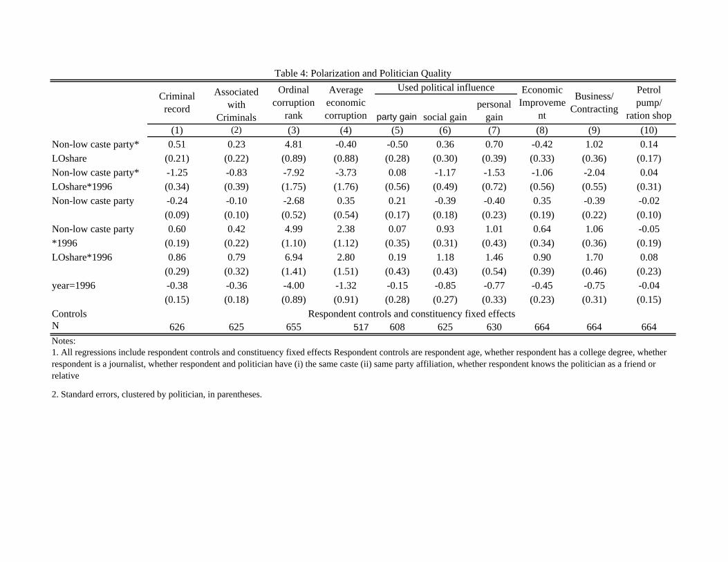
party gain social gain personal

gain(1) (2) (3) (4) (5) (6) (7) (8) (9) (10)

Non-low caste party* 0.51 0.23 4.81 -0.40 -0.50 0.36 0.70 -0.42 1.02 0.14LOshare (0.21) (0.22) (0.89) (0.88) (0.28) (0.30) (0.39) (0.33) (0.36) (0.17)Non-low caste party* -1.25 -0.83 -7.92 -3.73 0.08 -1.17 -1.53 -1.06 -2.04 0.04LOshare*1996 (0.34) (0.39) (1.75) (1.76) (0.56) (0.49) (0.72) (0.56) (0.55) (0.31)Non-low caste party -0.24 -0.10 -2.68 0.35 0.21 -0.39 -0.40 0.35 -0.39 -0.02

(0.09) (0.10) (0.52) (0.54) (0.17) (0.18) (0.23) (0.19) (0.22) (0.10)Non-low caste party 0.60 0.42 4.99 2.38 0.07 0.93 1.01 0.64 1.06 -0.05*1996 (0.19) (0.22) (1.10) (1.12) (0.35) (0.31) (0.43) (0.34) (0.36) (0.19)LOshare*1996 0.86 0.79 6.94 2.80 0.19 1.18 1.46 0.90 1.70 0.08

(0.29) (0.32) (1.41) (1.51) (0.43) (0.43) (0.54) (0.39) (0.46) (0.23)year=1996 -0.38 -0.36 -4.00 -1.32 -0.15 -0.85 -0.77 -0.45 -0.75 -0.04

(0.15) (0.18) (0.89) (0.91) (0.28) (0.27) (0.33) (0.23) (0.31) (0.15)ControlsN 626 625 655 517 608 625 630 664 664 664

Table 4: Polarization and Politician QualityOrdinal

corruption rank

Average economic corruption

Economic Improveme

nt

Used political influence

2. Standard errors, clustered by politician, in parentheses.

Notes:

Criminal record

Associated with

Criminals

1. All regressions include respondent controls and constituency fixed effects Respondent controls are respondent age, whether respondent has a college degree, whether respondent is a journalist, whether respondent and politician have (i) the same caste (ii) same party affiliation, whether respondent knows the politician as a friend or relative

Business/ Contracting

Petrol pump/

ration shop

Respondent controls and constituency fixed effects

party gainsocial gain

personal gain

(1) (2) (3) (4) (5) (6) (7) (8) (9) (10)winner 0.03 0.01 -0.12 0.17 0.11 0.00 -0.02 0.10 -0.04 0.10

(0.02) (0.03) (0.09) (0.08) (0.03) (0.04) (0.04) (0.03) (0.05) (0.03)winner*1996 0.01 0.07 0.39 0.27 0.05 0.05 0.22 0.14 0.12 -0.06

(0.04) (0.05) (0.13) (0.12) (0.05) (0.05) (0.06) (0.05) (0.06) (0.04)winner*reserved 0.01 0.07 0.35 0.43 -0.14 0.05 0.12 0.17 0.29 -0.20

(0.04) (0.05) (0.28) (0.25) (0.07) (0.07) (0.10) (0.07) (0.11) (0.08)winner*reserved* -0.04 -0.10 -0.75 -0.79 -0.02 0.07 -0.36 -0.44 -0.45 -0.011996 (0.11) (0.10) (0.38) (0.35) (0.11) (0.10) (0.14) (0.11) (0.19) (0.13)OthersN 1139 1131 1186 912 1053 1090 1111 1210 1210 1210

Table 5: Polarization and the Winner-Loser Corruption Gap

Ordinal corruption

rank

Average economic corruption

Economic Improvem

ent

Business/ Contracting

Used political influence

2. Respondent controls reported in notes to Table 4 are included in all regressions.

Notes

Criminal record

Associated with

criminals

1. Standard errors clustered by politician id reported in parentheses.

Respondent controls and constituency*year fixed effects

Petrol pump/

ration shop

(1) (2) (3) (4)Non-low caste party* -0.77 -0.06 -0.21 -0.05LOshare (0.41) (0.29) (0.23) (0.26)Non-low caste party* 0.99 -0.70 -0.06 -0.89LOshare*1996 (0.77) (0.59) (0.43) (0.86)Non-low caste party 0.62 0.26 0.02 -0.02

(0.25) (0.19) (0.10) (0.15)Non-low caste party -0.62 0.13 0.09 0.56*1996 (0.50) (0.40) (0.25) (0.56)LOshare*1996 -1.03 0.31 0.09 0.92

(0.65) (0.48) (0.39) (0.81)year=1996 0.72 0.03 -0.05 -0.60

(0.43) (0.33) (0.24) (0.53)ControlsN 647 638 664 589

winner 0.05 0.20 0.08 0.05

(0.06) (0.04) (0.05) (0.03)winner*1996 0.14 0.04 0.08 0.02

(0.07) (0.06) (0.06) (0.05)winner*reserved 0.44 -0.16 -0.01 -0.02

(0.11) (0.09) (0.12) (0.04)winner*reserved* -0.58 0.21 -0.24 -0.081996 (0.17) (0.15) (0.17) (0.10)OthersN 1181 1166 1210 1093

Respondent controls and constituency fixed effects

Other measures of politician quality

Table 6: Robustness Checks

Schools/ Hospital Associated

with Business

2. Respondent controls reported in notes to Table 4 are included in all regressions. 1. Standard errors clustered by politician id reported in parentheses.

Notes

Party position/ minister

Known for development

Respondent controls and constituency*year fixed effects

Panel B: Polarization and the Winner-Loser Corruption Gap

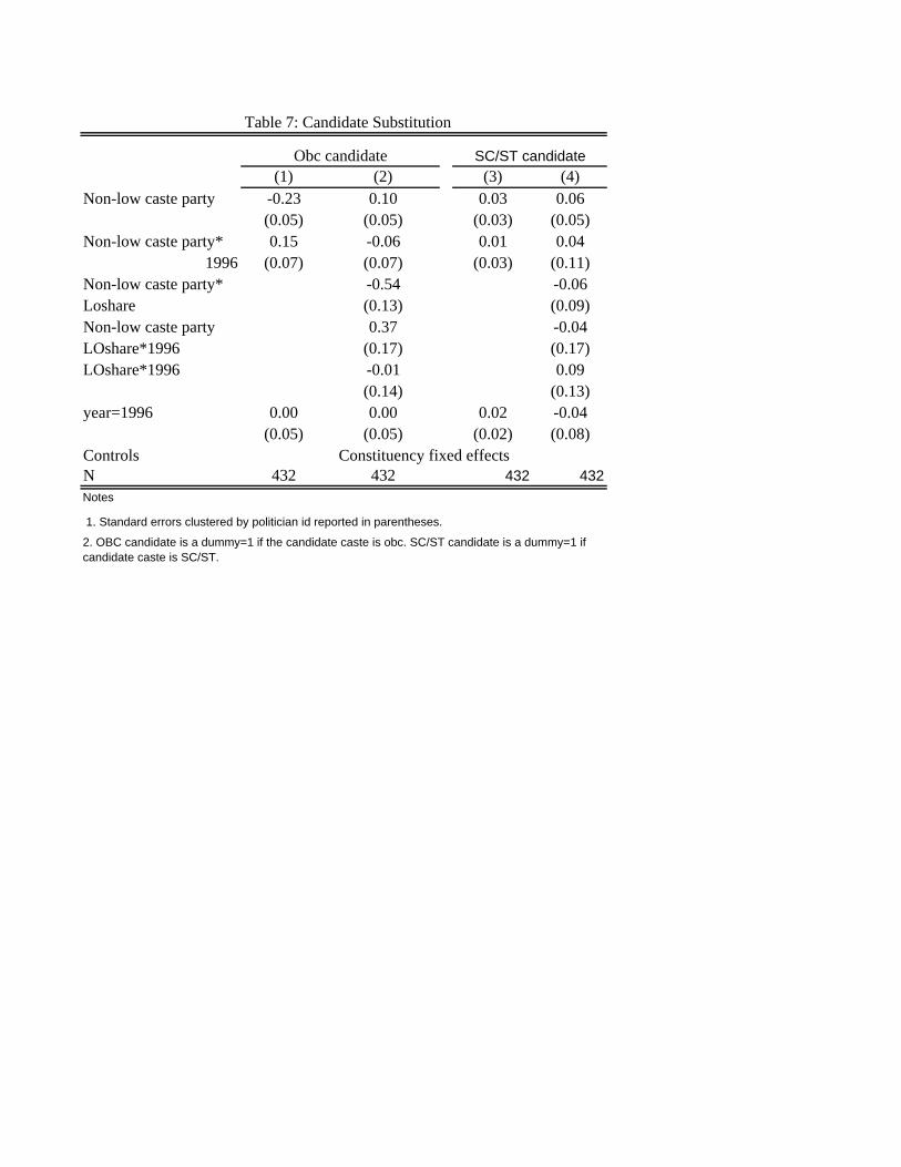
(1) (2) (3) (4)Non-low caste party -0.23 0.10 0.03 0.06

(0.05) (0.05) (0.03) (0.05)Non-low caste party* 0.15 -0.06 0.01 0.04

1996 (0.07) (0.07) (0.03) (0.11)Non-low caste party* -0.54 -0.06Loshare (0.13) (0.09)Non-low caste party 0.37 -0.04LOshare*1996 (0.17) (0.17)LOshare*1996 -0.01 0.09

(0.14) (0.13)year=1996 0.00 0.00 0.02 -0.04

(0.05) (0.05) (0.02) (0.08)ControlsN 432 432 432 432

Notes

Obc candidate

1. Standard errors clustered by politician id reported in parentheses.

2. OBC candidate is a dummy=1 if the candidate caste is obc. SC/ST candidate is a dummy=1 if candidate caste is SC/ST.

Constituency fixed effects

SC/ST candidate

Table 7: Candidate Substitution

1969 1980 1996Number of respondents 207 205 206

Age 70.73 59.33 47.13

Number of years has known 38.57 27.27 12.65politician

College educated 0.3 0.38 0.49

Journalist 0.49 0.5 0.49

Respondent and politician 0.168 0.186 0.16party match (match)

Politician is friend/relative 0.13 0.098 0.055(friend_relative)Was living in district during 0.92 0.88 0.85election asked about

Belongs to district being asked about 0.807 0.862 0.79

Appendix Table 1 : Summary Statistics on Respondents

overall 1969 1980 1996Petrol Pump

Number candidates compared 225 75 74 76

Matches (as % of total) 0.91 0.92 0.91 0.89% mismatches where ALL respondents disagree with objective data 0.33 0.33 0.43 0.25

750.8

0.53

0.13

1

0.86

Appendix Table 2: Comparison of Survey Corruption data with Objective verification

Criminal Cases (comparison of survey and Local Intelligence Unit (LIU) data)Number candidates comparedMatches (as % of total)

% mismatches where ALL respondents disagree with LIU

Mismatches when ALL survey respondents say candidate criminal but not LIU (as % of cases where LIU and survey disagree and LIU says no criminal case)

Mismatches when LIU says criminal and ALL survey respondents say not (as % of cases where LIU and survey disagree and LIU says criminal case)

Of these, number of cases where crime in LIU data is rioting as recorded by LIU

Panel A: winner sample (1) (2) (3) (4) (5) (6)Non-low caste party* 0.04 -0.08 -0.06 -0.23 -0.45 -0.36LOshare (0.98) (0.17) (0.74) (0.33) (0.37) (0.37)Non-low caste party* -2.99 -0.55 -1.08 -0.44 0.35 0.43LOshare*1996 (1.84) (0.30) (1.53) (0.55) (0.62) (0.65)Non-low caste party 0.11 0.02 0.34 0.27 0.37 0.32

(0.65) (0.09) (0.46) (0.20) (0.24) (0.22)Non-low caste party 2.28 0.35 0.70 0.34 -0.12 -0.18*1996 (1.23) (0.19) (1.00) (0.35) (0.43) (0.39)LOshare*1996 3.01 0.63 1.17 0.69 0.07 0.12

(1.53) (0.25) (1.33) (0.44) (0.45) (0.50)year=1996 -1.45 -0.27 -0.18 -0.22 0.20 0.16

(1.05) (0.15) (0.88) (0.28) (0.32) (0.31)ControlsN 648 624 530 659 659 630Panel B: Winner and winner 0.00 -0.01 0.09 0.03 -0.01 0.00

(0.10) (0.02) (0.08) (0.03) (0.04) (0.04)winner*1996 0.26 0.06 0.35 0.21 0.08 0.20

(0.14) (0.04) (0.12) (0.05) (0.06) (0.06)winner*reserved 0.27 0.04 0.49 0.22 0.22 0.24

(0.24) (0.03) (0.20) (0.09) (0.11) (0.08)winner*reserved* -0.69 -0.07 -0.77 -0.50 -0.39 -0.501996 (0.36) (0.11) (0.32) (0.12) (0.19) (0.12)ControlsN 1191 1147 937 1216 1216 1122Notes:

Appendix Table 3: Polarization and Politician Quality (using 1969 as base year)

Respondent controls and constituency fixed effects

Criminal record

Average economic corruption

Economic Improvement

Business/ Contracting

Used influence for personal gainOrdinal rank

1. Respondent controls are as listed in Table 4.

2. Standard errors, clustered by politician, in parentheses.

party gainsocial gain

personal gain

(1) (2) (3) (4) (5) (6) (7) (8) (9) (10)Sample: AgreedNon-low caste party* 0.45 0.51 -0.20 0.02 0.70 -0.15 1.39 0.06 -0.42 -0.38LOshare (0.17) (0.19) (0.53) (0.40) (0.57) (0.31) (0.41) (0.07) (0.23) (0.20)Non-low caste party* -0.79 -0.98 -0.54 -1.66 -3.77 -0.32 -1.98 0.16 -0.07 -0.15LOshare*1996 (0.28) (0.36) (1.05) (1.24) (1.24) (0.60) (0.65) (0.12) (0.46) (0.66)Non-low caste party -0.18 -0.28 -0.18 -0.27 -0.13 0.15 -0.54 0.04 0.09 0.15

(0.07) (0.10) (0.29) (0.26) (0.30) (0.18) (0.26) (0.03) (0.10) (0.11)Non-low caste party 0.39 0.54 0.58 1.48 2.56 0.25 0.95 -0.08 0.26 0.14*1996 (0.14) (0.18) (0.62) (0.85) (0.71) (0.35) (0.43) (0.07) (0.28) (0.42)LOshare*1996 0.70 0.73 0.40 1.75 3.87 0.65 1.68 -0.07 0.11 0.28

(0.25) (0.27) (0.75) (1.12) (1.03) (0.45) (0.54) (0.10) (0.42) (0.63)year=1996 -0.31 -0.37 -0.45 -1.44 -2.30 -0.33 -0.72 0.04 -0.23 -0.26

(0.12) (0.13) (0.45) (0.77) (0.61) (0.27) (0.37) (0.06) (0.26) (0.40)ControlsN 626 625 608 625 630 664 664 664 664 589

Appendix Table 4: Polarization and Politician Quality

Schools/ Hospital

Associated with

Business

2. All regressions include respondent controls in Table 4 and constituency fixed effects.

1. Each of the dependent variables is a dummy variable=1 only if the dummy variable=1 for all respondents asked about the candidate. Otherwise the dummy=0 for all respondents.

Sample: Agreed

Criminal record

Associated with

Criminals

3. Standard errors, clustered by politician, in parentheses.

Used political influence for Economic Improvem

ent

Business/ Contractin

g

Petrol pump/

ration shop

Notes:

Figure 1: Low Caste Legislators in UP state legislature (%)

0

5

10

15

20

25

30

35

40

45

50

55

1952 1957 1962 1967 1972 1977 1982 1987 1992 1997

Low caste OBC SC/SCT

Figure 2: Vote share of Low-caste parties in UP State Assembly Elections

0

10

20

30

40

50

60

1952 1957 1962 1967 1972 1977 1982 1987 1992 1997

Low caste

Notes: Low caste parties include SP and BSP. Data from Election Commission of India

Figure 3a: Winning likelihood of Non-low Caste Party: coefficient on Non-low Caste*year

-1.5

-1

-0.5

0

0.5

1

1.5

1967 1969 1971 1973 1975 1977 1979 1981 1983 1985 1987 1989 1991 1993 1995

Figure 3b: Winning likelihood of Non-low Caste party: coefficient on Non-low Caste party* LOshare*year

-2

-1.5

-1

-0.5

0

0.5

1

1967 1969 1971 1973 1975 1977 1979 1981 1983 1985 1987 1989 1991 1993 1995

Note: Figures 3a and 3b graph the coefficients on non-low caste party*year and non-lowcasteparty*Loshare*year

Party R

Party L

λ1 0 λ0

Q + λP = 0

Figure 4: Party position and voter utility

Figure 5: Increase in corruption across UP

0

0.1

0.2

0.3

0.4

0.5

0.6

0.7

econ

omic_im

prove

ment

Busines

s con

tracti

ng

petro

l pump

Criminal

assoc

iation

Crime re

cord

Corrupti

on rec

ord

1980 1996