parametric measurement of time-varying technical...

50 AGRICULTURAL ECO+OMICS REVIEW

Parametric Measurement of Time-Varying Technical Inefficiency: Results from Competing Models

Giannis Karagiannis and Vangelis Tzouvelekas* Abstract This paper provides an empirical comparison of time-varying technical inefficiency measures obtained from the econometric estimation of different specifications of the stochastic production frontier model. Specifically, ten different frontier model specifica-tions, which are most widely used in empirical applications, are estimated using a bal-anced panel data set from the Greek olive-oil sector, consisting of 100 farms observed during 1987-93 period. The empirical results indicate that both the magnitude and indi-vidual ranking of technical efficiency estimates differs considerably across models. Introduction

The use of panel data, repeated observations on each production unit, considerably enrich the econometric analysis of stochastic production frontier models and have sev-eral potential advantages over simple cross-section data. First, it offers a more efficient econometric estimation of the production frontier model.1 Second, it provides consistent estimators of firm inefficiency, as long as the time dimension of the data set is suffi-ciently large.2 Third, it removes the necessity to make specific distributional assump-tions regarding the one-sided error term associated with technical inefficiencies in the sample.3 Fourth, it does not require inefficiency to be independent of the regressors in-cluded in the production frontier.4 Fifth, it permits the simultaneous identification of both technical change and time-varying technical inefficiency, establishing thus a clear link between technical change, technical efficiency and productivity.5

Since the very first detailed discussion of efficiency measurement within the context of panel data (i.e., Pitt and Lee, 1981; Schmidt and Sickles, 1984), several alternative models have been progressively developed extending the existing methodological framework to account for different theoretical issues in empirical frontier modeling.

In empirical applications there has been no clear preference for one of the several al-ternative model specifications since no one has an absolute advantage over the others. Moreover, the choice among them is further complicated by the fact that, in general, they are not nested to each other which implies that there are no statistical criteria to discriminate among them.6 Hence, the choice for the appropriate model of pooling is based on a priori grounds related with the particular objectives of each empirical appli-cation or with data availability as well as the underlying hypotheses for each production * Giannis Karagiannis: Dept. of Economics, University of Ioannina, Greece Corresponding author: Vangelis Tzouvelekas: Dept. of Economics, University of Crete, Greece,

University Campus, 74 100 Rethymno, Greece Phone: +30-831-77426; Facsimile: +30-831-77406; e-mail: [email protected] or [email protected]

2009, Vol 10, +o 1 51

frontier model. However, empirical evidence suggests that the economic optima, includ-ing efficiency, are sensitive to the choice of the estimation technique. It is evident, therefore, that all these necessitate considering the comparative performance of these models in real world applications.

In the empirical literature on frontier modeling with panel data, the issues of model specification and selection of estimation technique have not been explored in detail. The objective of this paper is to contribute in the existing literature providing a more com-prehensive comparison of the most widely applied model specifications used to measure output-oriented time-varying technical inefficiency with panel data. The paper explores the sensitivity of obtained technical inefficiency estimates to the choice of the model of pooling, while maintaining an identical data set and retaining the same assumptions about the underlying production technology. In particular ten of the most widely applied frontier models are estimated and compared using a balanced panel data set from the Greek agricultural sector consisting of 100 olive-growing farms observed over the 1987-93 period.

The rest of the paper is organized as follows: In the next section a brief review of studies on the effect of the choice for the model of pooling on efficiency measurement is presented. Section 3 provides a brief review of alternative model specifications used to measure time-varying technical inefficiency with panel data. The data used in the present study and the empirical model are presented in the fourth section. The empirical results and the comparative performance of alternative models considered herein are discussed in the fifth section. Finally, section 6 summarizes and concludes the paper.

A Review of Alternative Models Pitt and Lee (1981) and Schmidt and Sickles (1984) first specified a panel data ver-sion of the stochastic frontier production function with multiplicative disturbance of the form: ( ), ; itε

it ity f x t β e= (1) where, yit is the output of the production unit i (i=1, 2, …, G) at time t (t=1, 2, …, T), xit is the matrix of j inputs, t is a time index that serves as a proxy for technical change, β are the parameters to be estimated and εit is the error term composed of two independent elements such that: it it itε v u≡ − (2) The symmetric component, vit , is identically and independently distributed and cap-tures random variation in output resulting from factors outside the control of the farm (weather, diseases, machine breakdown, etc.) as well as measurement errors and left-out explanatory variables. The one-sided component, uit ≥ 0, reflects technical inefficiency relative to the stochastic frontier of the ith firm at year t. In this case, technical ineffi-ciency is defined in an output-expanding manner (Debreu-type) as the discrepancy be-tween a firm’s actual output and its potential output, using the same amount of inputs employed with the frontier technology.


A number of methods are available for the econometric estimation of (1), giving rise to alternative measures of time-varying technical inefficiency. A summary of the most widely applied models along with their main features is presented in Table 1 and dis-cussed in the following sections. The Fixed Effects Model In the fixed effects model, individual technical inefficiency is treated as an unknown fixed parameter to be estimated. Following Schmidt and Sickles (1984) and assuming that technical inefficiency is time-invariant, a general fixed-effects production frontier model can be written as: ( )0 , ;it i it ity β f x t β v= + +

where 0 0i iβ β u= − (3) and vit is an iid error term uncorrelated with the regressors. No distributional assump-tions are required for ui which is assumed to be correlated with the regressors or with vit. Consistent estimators of β’s are obtained by applying either OLS to the within group deviations from the means of yit and xit

7 or by using firm-specific dummy variables for the intercept terms. Then, individual time-invariant technical inefficiency is obtained by employing the normalization suggested by Schmidt and Sickles (1984) which en-sures that 0�

iu ≥ i∀ . First, the maximum intercept term is obtained to indicate the fully efficient firm in the sample { }0 0max

� �

iiβ β= and then ui are recovered as 0 0

� �

�

i iu β β= − . Producer-specific but time-invariant technical inefficiency is then given by

( )exp �

i iTE u= − . A considerable advantage of the fixed effects model lies in the fact that the statistical properties of the estimators obtained do not depend on the assumption of uncorrelated-ness of the regressors with the firm effects. Consistent estimates of firm effects can be obtained as either G or T grows to infinity and the consistency property does not re-quire that the ui be uncorrelated with the regressors. The maintained assumption that technical inefficiency is constant through time is rather restrictive in a competitive economic environment particularly when the number of time periods is large. It is possible within the context of fixed effects model to relax this assumption at the cost, however, of additional parameters to be estimated. Obvi-ously it is not possible to obtain estimates of producer and time specific intercepts (GxT) due to insufficient degrees of freedom. Cornwell et al., (1990) and Lee and Schmidt (1993) addressed this problem suggesting two distinct approaches for the estimation of both producer and time specific technical efficiency. These models are not directly comparable in the sense that neither includes the other as a special case. First, Cornwell et al., (1990) (hereafter CSS) assumed that technical inefficiency fol-lows a quadratic pattern over time. Specifically, they suggest the following formulation for individual effects (Model 1.1):

2009, Vol 10, )o 1

53

Table 1. Models of Time-Varying Technical Efficiency

Pattern of TE across: Model

Estimation Method

Distributional Assumption

Independence of X and u

Producers Time

Subsumes

Cornwell et al., (1990) LSDV, GLS, EIV

No Yes/No

1 Different

Different None

Lee and Schmidt (1993) LSDV, GLS

No Yes/No

1 Common Different

Kumbhakar (1990) Kumbhakar and Heshmati (1995)

Mixture of GLS and ML

Yes Yes

Different Different

None

Battese and Coelli (1992) ML

Yes Yes

Common Common None

Cuesta (2000) ML

Yes Yes

Different Common Battese&Coelli (1992)

Battese and Coelli (1995) ML

Yes Yes

Different Different

None Huang and Liu (1994)

ML Yes

Yes Different

Different Battese&Coelli (1995) 1 Both hypotheses are valid according to the adopted estimation method.


20 1 2it i i iβ δ δ t δ t= + + (4)

where, δi1, δi2 and δi3 are the ( x3) unknown parameters to be estimated. If 1 2 0i iδ δ= = i∀ , then technical efficiency is time-invariant, while when 1 1iδ δ= and 2 2iδ δ= i∀ then technical efficiency is time-varying following, however, the same pattern for all producers.8 CSS suggest to estimate the model in (4) following either an one or a two step procedure.

When /T is relatively small, one can adopt an one-step procedure where uit are in-cluded directly in (3) using dummy variables. However, in this case it is not possible to distinguish between technical change and time-varying technical efficiency if both are modeled via a simple time-trend. In the two-step procedure, OLS estimates on the within group deviations are obtained for β’s and then the residuals for each producer in the panel are regressed against time and time-squared as in (4). In both cases time-varying technical inefficiency is obtained following the same normalization for each year of the panel as in the time-invariant case which ensures that 0�

itu ≥ ,i t∀ .9 That is, ( )expit itTE u= − where { }max

� �

�

it it itiu β β= − .

The advantages of this specification are its parsimonious parameterization regardless of frontier functional form, its straightforward estimation, its independence of distribu-tional assumptions, and that it allows inefficiency to vary across firms and time. More-over, since the expression in (4) is linear to its parameters (δ’s), the statistical properties of firm effects are not affected. However, a shortcoming of (4) is that it is quite restric-tive in describing the temporal pattern of technical inefficiency which is assumed to be deterministic.

Lee and Schmidt (1993) (hereafter LS) proposed an alternative formulation which is similar to Baltagi and Griffin (1988) model of technical change. Specifically, u’s in (3) are specified as (Model 2.1): ( )it iu δ t u= ⋅ (5) where ( )δ t is an appropriate set of dummy variables δt, the parameters of which need to be estimated. The model in (5) can be estimated in a single stage by including uit di-rectly into the production frontier in (3) imposing the normalization that δ1=1.10 In case however, that technical change is modeled with a multiple time-trend again it is not pos-sible to distinguish it’s effect from that of time-varying inefficiency. Once the δt’s and ui’s are estimated, farm and time specific technical efficiency is obtained as:

( )expit itTE u= − where { } ( )max� �

� �

it t i t iiu δ u δ u= − .

If 1tδ = t∀ then the model collapses to the time-invariant case. Despite its non-linearity, this specification is attractive as it does not impose any functional specifica-tion on the temporal pattern of inefficiency. It is applicable when the time span of the data set is small. One disadvantage of (5) is that the temporal pattern of inefficiency, not the magnitude, is assumed to be the same for all firms. Although in cases of small num-ber of time-periods this hypothesis seems to be appropriate, when the number of time-periods is large one would expect the temporal pattern of technical inefficiency to vary across firms (Kumbhakar et al., 1997).

2009, Vol 10, )o 1 55

The Random Effects Model In the random effects model, instead of working conditionally on the individual tech-nical inefficiency, one can takes explicitly into account it’s stochastic nature.11 This modification in the assumptions for individual technical efficiency has the virtue of al-lowing us to include time-invariant regressors in the model at the expense, however, of assuming that X and ui are not correlated. This leads to a stochastic frontier model taking into account the panel structure of the data: ( ) ( ) ( )0 , ;it i it it i iy β E u f x t β v u E u = − + + − − (6) The model in (6) can be estimated by making no use of distributional assumption about the one-sided error term using the standard two-step GLS method. In the first-step OLS residuals are used to obtain the two variance components by any of the several methods suggested in the literature. Then feasible GLS parameter estimates are obtained by applying OLS to the following transformed equation: ( ) ( ), ;it it i i it it ity ψy β ψβ f x ψx t β v − = − + − + (7)

where ( )21 vψ σ σ= − . The above estimator is equivalent to within estimator when 1ψ = .

The GLS estimator is consistent as either 3 or T tends to infinity given that no-correlation between the regressors and the error terms is assumed.12 If the firm effects are correlated with the independent variables, the within estimator is GLS, regardless of whether these effects are random or fixed (Greene, 1993). On the other hand, when in-dividual effects and the regressors are uncorrelated, GLS is more efficient than the within, except in the cases of relatively small samples. However, consistent estimates of firm effects require � →∞ .

The main advantage of GLS estimator relative to the within estimator is not statisti-cal efficiency of the parameter estimates, but rather the ability of the random effects model to allow for time-invariant firm-specific variables in the regression equation. Thus, the random effects seems to be attractive in the framework of production frontier model since it takes into account the random structure of farm efficiencies and does not share the disadvantage of the fixed effects. The price to be paid, however, is the uncor-relatedness between the firm effects and the regressors.

Time-variant technical inefficiency is modeled in the same way as in the case of fixed effects model following either CSS (Model 1.2) or LS (Model 2.2) approaches. Apart of the above specifications, in the context of random effects model, Kumbhakar and Heshmati (1995) (hereafter KH) proposed an alternative specification for estimating time-varying technical efficiency which is a mixture of ML and GLS methods. They suggested that technical inefficiency might be decomposed into a persistent (time-invariant) and a time-varying component (Model 3).13 That is, it i itu µ ξ= + (8) where µi is the persistent component, which is only producer-specific, and ξit is the component that is both producer- and time-specific. This model is estimated in two steps: the persistent component µi is estimated after the GLS estimation of (3) using

56 AGRICULTURAL ECO)OMICS REVIEW

the normalization suggested initially by Schmidt and Sickles (1984), while in the second step the residual component ξit is estimated as a one-sided error component using ei-ther ML or a method of moments approach. A disadvantage of this specification is that if there is any persistent time-specific inefficiency, it is masked into technical change (Kumbhakar and Heshmati, 1995).14 Further, it is not possible to test over the temporal variation of technical efficiency. The Efficient Instrumental Variable Estimator

The uncorrelatedness between individual effects and the regressors is rather a strong assumption. The GLS estimates are inconsistent if technical inefficiencies are correlated with the regressors. CSS resolved the problem suggesting an efficient instrumental vari-able estimator (EIV) that is consistent when efficiencies are correlated with the regres-sors allowing at the same time the inclusion of time invariant regressors into the frontier model. However, the number of time-varying regressors that are uncorrelated with the one-sided error term must be at least as large as the number of time invariant regressors that are correlated with the one-sided error term (Schmidt and Sickles, 1984).

A problem arises however with the choice of variables entering into the model as in-struments. A convenient choice for instruments could be the exogenous variables ex-pressed as deviations from their mean plus a subset of them that is assumed to be uncor-related with individual effects ui (Breusch et al., 1989). The estimation of individual technical efficiencies is done following CSS two-step approach (Model 1.3). The only difference is that different sets of residuals are used. Hence, in that way consistent and efficient estimators are obtained when the individual effects are correlated with the ex-planatory variables, while the stochastic nature of the production frontier model is main-tained. Battese and Coelli (1992) ML Estimator (Model 4.1) The Battese and Coelli (1992) (hereafter BC92) is an extension of Battese and Coelli’s (1988) model into panel data setting. Specifically, their model can be expressed as: ( )0 , ;it it it ity β f x t β v u= + + −

and ( )( ) η τ Tit iu e u

− −

= (9) where, uit is an iid non-negative error term following a truncated normal distribution,

( )2, u� µ σ , independent of the random noise and the regressors; η is a unknown scalar parameter to be estimated which introduces time-varying technical inefficiency and;

[ ]1, 2, ..., Tτ∈ is the set of time periods among the T periods for which observations for the ith producer are obtained.15 Thus, in the above model time-varying efficiency is assumed to follow an exponen-tial function of time, involving only one parameter to be estimated. Technical ineffi-ciency either increases at a decreasing rate, when η is greater than zero, or decreases at an increasing rate when η is less than zero. If η is equal to zero then the time-invariant model is obtained. In case that µ=0 then the model collapses to Aigner’s et

2009, Vol 10, )o 1 57

al., (1977) half-normal case with technical inefficiency being time-varying. For the es-timation of ui, BC92 extended the predictor of Jondrow et al., (1982) to panel data, which is consistent as T grows to infinity.16 The main drawback of BC92 model is the need to assume a priori a specific distribu-tion for the one-sided error term. Further, (9) presumes a quite restrictive temporal pat-tern of technical efficiency, due to its exponential parameterization the magnitude of which is assumed to be the same for all producers (Kumbhakar et al., 1997). Cuesta (2000) ML Estimator (Model 4.2) Cuesta (2000) (hereafter CT) generalized BC92 model to allow for more flexibility in the way that technical inefficiency changes over time. Specifically, he proposed a model with producer-specific patterns of time-varying technical inefficiency defined as: ( )( ) iη τ T

it iu e u− −

= (10) where, ηi are producer-specific parameters capturing temporal variation of individual technical efficiency ratings and ui is a positive truncation of the ( )2,� µ σ distribution. In that way technical inefficiency evolves over time at a different rate among producers in the sample. In case that µ=0 the model reduces to Aigner’s et al., (1977) half-normal model, while when iη θ= i∀ the model collapses to BC92 model with a common time-pattern of technical inefficiency across producers. Finally, if 0iη = i∀ technical inefficiency is time-invariant. Besides temporal variations of technical inefficiency are produce-specific, the above model shares the same exponential parameterisation with BC92 model which is rather restrictive. Further, as any other ML model independence between inputs and technical efficiency is assumed. Cuesta (2000) provides in the appendix the corresponding likeli-hood function and the conditional expectation of uit. Battese and Coelli (1995) ML Estimator (Model 5.1) Battese and Coelli (1995) (hereafter BC95) extending the approach put forward by Kumbhakar et al., (1991) and Reifschneider and Stevenson (1991), suggested that the technical inefficiency effects, uit, could be replaced by a linear function of explanatory variables reflecting producer-specific characteristics. In this way, every producer in the sample faces its own frontier, given the current state of technology and its physical en-dowments, and not a sample norm. The technical inefficiency effects are assumed to be independent, non-negative, truncations (at zero) of normal distributions with unknown variance and mean. Specifically,

it1

uM

o m mit itm

δ δ z ω=

= + +∑ (11)

where, zmit are the producer and time specific explanatory variables (e.g., socio-economic, demographic) associated with technical inefficiencies; δ0 and δm are pa-rameters to be estimated and;17 ωit is a random variable with zero mean and variance


σ2, truncated at Mm mitm δ z−∑ from below, or equivalently ~itu ( )2,

Mm mitm δ z σ∑

truncated at zero from below. A simple time trend can also be included as part of the z vector and it can be interpreted as the change in a linear fashion of technical ineffi-ciency over time. In case that 0mδ = m∀ , the specification considered by Stevenson (1980) is im-plied, where ui follows a truncated normal distribution. If, however, 0 0mδ δ= = m∀ , the original Aigner et al., (1977) half-normal specification is obtained. In the later case, the technical inefficiency effects are not related to the explanatory variables, while in both cases technical inefficiency is assumed to be tome-invariant. The parameters of both the stochastic frontier and inefficiency effects models can be consistently estimated by maximum likelihood method.18 The above formulation of inefficiency effects has several advantages. First, it identi-fies separately time-varying technical efficiency and technical change by using a single-stage estimation procedure, as long as the inefficiency effects are stochastic and having a known distribution. Second, it is not necessary to assume that technical efficiencies follow a specific time pattern, common to all firms in the sample, as in BC92 model. The magnitude of the temporal pattern for technical inefficiency is determined by all variables included in the inefficiency effects model. Third, it identifies consistently the factors influencing technical efficiency in a single stage.19 Fourth, relaxes the constant mode property of the truncated normal distribution, by permitting the mode to be a function of the z exogenous producer-specific variables. However, still the variances, σ2 are assumed to be the same across individuals.20 Huang and Liu (1994) ML Estimator (Model 5.2) Huang and Liu (1994) (hereafter HL) extended BC95 model specification introduc-ing the non-neutral stochastic frontier model in a sense that the MRTS differs between the average and best practice frontier. In their specification, apart of the socio-economic and demographic variables, conventional inputs are also appear in the one-sided error term, shifting thus the efficient frontier in a non-neutral way. According to HL a ration-ale behind that is that producers gain relative more experience over time with respect to some inputs, than others. Further, governmental intervention or institutional regulations may affect different the relative performance of certain inputs. To capture these effects, interaction terms between producer-specific variables (zmit) and input quantities are also included in the technical inefficiency effects itu . Thus, (11) may be reformulated as:

01 1 1

M M Jit m mit mj mit jit it

m m ju δ δ z δ z x ω

= = =

= + + +∑ ∑∑ (12)

where the parameters δmj are reflecting the appropriate interactions between producer-specific variables and input quantities. In this case, time-varying technical inefficiency also depends on the levels of inputs used, as the frontier of each firm shifts differently over time. Notice that in the case where 0mjδ = m∀ , the above model in (12) is re-duced to the BC95 specification, while when 0m mjδ δ= = m∀ and 0 0m mjδ δ δ= = = m∀ the model reduces to Stevenson’s (1980) and Aigner’s et al., (1977) specification.

2009, Vol 10, )o 1 59

Data and empirical model The data used in this study were extracted from a survey undertaken by the Institute

of Agricultural Economics and Rural Sociology, Greece. Our analysis focuses on a sample of 100 olive-growing farms, located in the four most productive regions of Greece (Peloponissos, Crete, Sterea Ellada and Aegean Islands). Observations were ob-tained on annual basis for the period 1987-1993. The sample was selected with respect to production area, the total number of farms within the area, the number of olive trees on the farm, the area of cultivated land and the share of olive oil production in farm out-put.

The unknown production structure of olive-growing farms is approximated by a sin-gle-output multiple-input translog production frontier. Specifically, the production fron-tier assuming that a time-trend representation of technical change may be non-neutral and scale augmenting, has the following form:21

20 1 2

1 1 1 1

1 12 2

J J J Jit j jit jk jit kit j jit it

j j k jy β α t α t β x β x x α x t ε

= = = =

= + + + + + +∑ ∑∑ ∑ (12)

where, i=1, 2, …, 3 denotes cross-section units; t=1, 2, …, T denotes time periods; j,k=1, 2, …, J denote the inputs used.

The dependent variable is the annual olive oil production measured in kilograms. The aggregate inputs included as explanatory variables are: (a) total labor, comprising hired (permanent and casual), family and contract labor,

measured in working hours. It includes all farm activities such as plowing, fertiliza-tion, chemical spraying, harvesting, irrigation, pruning, transportation, administra-tion and other services;

(b) fertilizers, including nitrogenous, phosphate, potash, complex and others, measured in kilograms;

(c) other expenses, consisting of pesticides, fuel and electric power, irrigation taxes, depreciation, and other miscellaneous expenses, measured in drachmas (constant 1990 prices);

(d) land, including only the share of farm’s land devoted to olive-tree cultivation meas-ured in stremmas (one stremma equals 0.1 ha).

The farm specific characteristics included in the inefficiency effects models (Models 5.1 and 5.2) are: (a) farmer’s age and the age-squared in years; (b) farmer’s education in years of schooling and; (c) a simple time trend.

Aggregation over the various components of the above input categories (except for land input) was conducted using Divisia indices with cost shares serving as weights. To avoid problems associated with units of measurement, all variables were converted into indices, with the basis for normalization being the representative olive-growing farm. The choice of the representative farm was based on the smallest deviation of the vari-ables (i.e. output and input levels) from the sample means.


Empirical results Production Frontier Estimates

Parameter estimates of the translog production frontier arising from the econometric estimation for each of the alternative models presented in the previous section are shown in Tables 2 through 5. For all models the estimated first-order parameters (βi) are having the anticipated (positive) sign and magnitude (being between zero and one), whereas the bordered Hessian matrix of the first and second-order partial derivatives is negative semi-definite indicating that all regularity conditions (i.e., positive and dimin-ishing marginal products) are valid at the point of approximation. Thus, all nine models result in a well-behaved production frontier function.

The goodness of fit, measured either by the adjusted R-squared (Models 1.1 through 2.2) or by the log of the likelihood function (Models 4.1 through 5.2), is satisfactory in all models. Restrictive structures of production, such as homotheticity, homogeneity, linear homogeneity, additive and strong separability are rejected by the likelihood ratio test at the 5% level of significance (see Table 6).22 Moreover, restricted functional forms, such as Cobb-Douglas, with and without assuming Hicks- neutral technical change, are also rejected at the 5% level of significance.

In all ML models the ratio parameter, γ, is positive and significant at the 1% level, implying that farm-specific technical efficiency is important in explaining the total vari-ability of output produced (the value of γ ranges from a minimum of 0.613 in Model 4.2 to a maximum of 0.960 in Model 5.1). The same is also true in GLS models (Models 1.2 and 2.2) as variance of the error component is much higher (σu) than that of the random error (σv). The statistical significance of modeling farm effects within the stochastic frontier models is further examined and the results are presented in Tables 7 and 8.

First, the traditional average response function does not adequately represents the structure of Greek olive-growing farms in all nine models. Specifically, in Models 1.1 and 2.1 the null hypothesis that 0 iiu = ∀ is rejected at 5% level of significance using the conventional F-test.23 The same is true for Models 1.2, 1.3 and 2.2 as the null hy-pothesis of 2 0uσ = is rejected using the LM-test at the same level of significance.24 On other hand, in all ML models the corresponding statistical testing using LR-test25 also support the existence of the stochastic frontier function (see hypotheses 1, 3 and 11 in Table 8). For Models 5.1 and 5.2 this true regardless of whether farm inefficiency ef-fects are present or absent from the production frontier model (see hypotheses 4 and 7 in the same Table).

Next, technical inefficiency was found to be time-varying in all model specifica-tions.26 For Models 1.2 through 1.3 the null hypothesis that 1 20 0i iδ δ= ∧ = i∀ is re-jected at 5% level of significance (see Table 7). As well, the hypotheses that the tempo-ral pattern of technical inefficiencies is common across farms or that it does not follow a quadratic trend over time are both rejected at the same level of statistical significance (i.e., 1 1 2 2 i iδ δ δ δ= ∧ = and 2 0iδ = i∀ ). Models 2.1 and 2.2 also reveal time-varying individual technical inefficiency as the hypothesis of 1tδ = t∀ is rejected (see Table 7).

The temporal pattern of technical inefficiencies was found to be time-variant in all ML models as the relevant hypotheses are rejected at the 5% level of significance (hy-

2009, Vol 10, )o 1 61

Table 2. Generalized Least Squares and Efficient Instrumental Variable Estimators of the Translog Production Frontier

Model 1.1 Model 1.2 Model 1.3 Variable Parameter StdError Parameter StdError Parameter StdError

β0 – – –0.0081 (0.0024)* 0.0061 (0.0015)*

βL 0.3140 (0.0240)* 0.3019 (0.0493)* 0.2767 (0.0278)*

βF 0.0922 (0.0277)* 0.1126 (0.0559)** 0.1856 (0.0309)*

βC 0.1618 (0.0133)* 0.1841 (0.0290)* 0.1455 (0.0145)*

βA 0.3961 (0.0385)* 0.3770 (0.0685)* 0.4151 (0.0248)*

α1 0.1201 (0.0369)* 0.1022 (0.0368)* 0.1033 (0.0365)*

α2 0.0164 (0.0178) 0.0371 (0.0413) –0.0640 (0.0182)*

βLF 0.0141 (0.0266) –0.0159 (0.0424) 0.0448 (0.0293) βLC –0.0322 (0.0137)** –0.0608 (0.0300)** –0.0866 (0.0169)*

βLA –0.0815 (0.0351)** –0.0933 (0.0462)** 0.0784 (0.0330)**

βLL 0.0959 (0.0162)* 0.1110 (0.0313)* 0.0846 (0.0214)*

βFC 0.0594 (0.0149)* 0.0546 (0.0275)** 0.0592 (0.0146)*

βFA –0.0064 (0.0024)* 0.0665 (0.0214)* –0.0380 (0.0383) βFF –0.0025 (0.0182) –0.0299 (0.0130)** 0.0076 (0.0158) βCA 0.0190 (0.0205) 0.0100 (0.0337) 0.0439 (0.0210)**

βCC 0.0115 (0.0053)** 0.0211 (0.0100)** 0.0102 (0.0046)**

βAA –0.0740 (0.0324)** –0.0377 (0.0542) –0.1202 (0.0302)*

αL –0.0132 (0.0229) –0.0350 (0.0452) 0.0142 (0.0240) αF –0.0512 (0.0253)** 0.0019 (0.0459) –0.0063 (0.0285) αC 0.0562 (0.0120)* 0.0679 (0.0255)* 0.0428 (0.0147)*

αA –0.1049 (0.0269)* –0.0901 (0.0258)* –0.1546 (0.0273)*

2R 0.8976 0.8976 0.7592 σv – 0.0564 0.0342 σu – 0.2341 0.1782

* significant at the 1 per cent level; ** significant at the 5 per cent level. Where, L stands for labor, F for fertilizers, C for other expenses, A for area and T for time. Model 1.1: Cornwell et al., (1990) fixed effects model, Model 1.2: Cornwell et al., (1990) random effects

model, Model 1.3: Cornwell et al., (1990) EIV estimator.


Table 3. Generalized Least Squares and Efficient Instrumental Variable Estimators of the Translog Production Frontier

Model 2.1 Model 2.2 Variable Parameter StdError Parameter StdError

β0 – – -0.2134 (0.0299)*

βL 0.2974 (0.0294)* 0.3140 (0.0983)*

βF 0.1995 (0.0335)* 0.0922 (0.0453)**

βC 0.2157 (0.0157)* 0.1618 (0.0345)*

βA 0.4523 (0.0245)* 0.3961 (0.0987)*

α1 0.0519 (0.0132)* 0.0300 (0.0123)**

α2 -0.0403 (0.0178)** 0.0164 (0.0365) βLF 0.0475 (0.0316) 0.0115 (0.0516) βLC -0.0949 (0.0178)* -0.0740 (0.0312)**

βLA 0.0783 (0.0392)** 0.0141 (0.0132) βLL 0.0939 (0.0220)* -0.0322 (0.0143)**

βFC 0.0643 (0.0159)* -0.0815 (0.0342)**

βFA -0.0406 (0.0411) 0.0959 (0.0265)*

βFF 0.0082 (0.0170) 0.0594 (0.0123)*

βCA 0.0480 (0.0223)** -0.0064 (0.0452) βCC 0.0121 (0.0056)** -0.0025 (0.0092) βAA -0.1254 (0.0293)* 0.0190 (0.0542) αL -0.0129 (0.0257) -0.0132 (0.0452) αF -0.0074 (0.0309) -0.0512 (0.0459) αC 0.0458 (0.0158)** 0.0206 (0.0098)**

αA -0.1636 (0.0290)* -0.1049 (0.0325)*

2R 0.9713 0.8976 σv – 0.0564 σu – 0.2341

* significant at the 1 per cent level; ** significant at the 5 per cent level. Where, L stands for labor, F for fertilizers, C for other expenses, A for area and T for time. Model 2.1: Lee and Schmidt (1993) fixed effects model, Model 2.2: Lee and Schmidt (1993) random

effects model.

2009, Vol 10, )o 1 63

Table 4. Maximum Likelihood Estimates of the Translog Production Frontier Model 4.1 Model 4.2 Model 5.1 Model 5.2 Variable

Param. StdError Param. StdError Param. StdError Param. StdError β0 0.2389 (0.0544)* 0.1102 (0.0079)* 0.2371 (0.0394)* 0.2442 (0.0486)*

βL 0.2941 (0.0478)* 0.3751 (0.1134)* 0.3105 (0.0486)* 0.2923 (0.0487)*

βF 0.1173 (0.0543)** 0.1316 (0.0257)* 0.1041 (0.0357)* 0.1171 (0.0551)**

βC 0.1893 (0.0280)* 0.1622 (0.0171)* 0.1856 (0.0292)* 0.1864 (0.0292)*

βA 0.3829 (0.0653)* 0.3992 (0.1234)* 0.3980 (0.0639)* 0.4250 (0.0626)*

α1 0.0276 (0.0102)* 0.0735 (0.0063)* 0.0656 (0.0239)* 0.0552 (0.0191)*

α2 0.0202 (0.0423) -0.0258 (0.4337) 0.0328 (0.0452) 0.0268 (0.0445) βLF -0.0175 (0.0413) -0.1087 (0.0395)* -0.0403 (0.0448) -0.0447 (0.0182)**

βLC -0.0620 (0.0291)** -0.1279 (0.0525)** -0.0571 (0.0231)** -0.0506 (0.0206)**

βLA -0.0912 (0.0360)** -0.1215 (0.0244)* -0.0948 (0.0452)** -0.1013 (0.0475)**

βLL 0.1079 (0.0308)* 0.1433 (0.0297)* 0.1246 (0.0332)* 0.1175 (0.0336)*

βFC 0.0543 (0.0268)** 0.1645 (0.0383)* 0.0825 (0.0290)* 0.0772 (0.0290)*

βFA 0.0635 (0.0283)** 0.0283 (0.3339) 0.0927 (0.0459)** 0.1074 (0.0517)**

βFF -0.0252 (0.0290) -0.0220 (0.2025) -0.0460 (0.0230)** -0.0500 (0.0219)**

βCA 0.0098 (0.0329) 0.0611 (0.0234)* -0.0012 (0.0351) -0.0020 (0.0360) βCC 0.0228 (0.0101)** 0.0354 (0.0164)** 0.0119 (0.0047)** 0.0125 (0.0057)**

βAA -0.0376 (0.0525) -0.0245 (0.5312) -0.0318 (0.0534) -0.0279 (0.0519) αL -0.0335 (0.0444) -0.0270 (0.2800) -0.0224 (0.0475) -0.0212 (0.0475) αF 0.0032 (0.0450) 0.0166 (0.6857) -0.0023 (0.0497) -0.0057 (0.0481) αC -0.0693 (0.0250)* 0.0527 (0.0127)* 0.0725 (0.0267)* 0.0739 (0.0264)*

αA -0.1005 (0.0457)** -0.0416 (0.0132)* -0.0710 (0.0326)** -0.0688 (0.0254)*

Ln(θ) -380.179 -401.924 -407.747 -424.576 σ2 0.2483 (0.0344)* 0.7382 (0.0879)* 0.2214 (0.0716)* 0.8195 (0.2276)*

γ 0.7864 (0.2009)* 0.6130 (0.0584)* 0.9608 (0.0235)* 0.8457 (0.0526)*

η 0.0478 (0.0213)** – – – – – – µ -0.8972 (0.2926)* -1.9622 (0.6299)* – – – –

* significant at the 1 per cent level; ** significant at the 5 per cent level. Where, L stands for labor, F for fertilizers, C for other expenses, A for area and T for time.Model 4.1:

Battese and Coelli (1992) truncated half-normal model, Model 4.2: Cuesta (2000) truncated half-normal model, Model 5.1: Battese and Coelli (1995) inefficiency effects model, Model 5.2: Huang and Liu (1994) non-neutral stochastic frontier model.


Table 5. Maximum Likelihood Estimates of the Inefficiency Effects Model Model 5.1 Model 5.2 Variable Parameter StdError Parameter StdError

δ0 -12.7221 (4.4883)* -2.5947 (1.1495)**

δAge -3.0142 (1.3547)** -0.6102 (0.2352)*

δEdu -0.7381 (0.3484)** -0.2369 (0.1003)**

δT -1.5992 (0.4598)* -0.4092 (0.1822)**

δAgeL – – 1.8950 (0.8755)**

δAgeF – – 0.3470 (0.5566) δAgeC – – -0.6484 (0.2537)**

δAgeA – – -1.3048 (0.6071)**

δEduL – – 0.1262 (0.1002) δEduF – – -0.5940 (0.2532)**

δEduC – – 0.1424 (0.1096) δEduA – – -0.7581 (0.3385)**

* significant at the 1 per cent level; ** significant at the 5 per cent level. Where, L stands for labor, F for fertilizers, C for other expenses, A for area, T for time, AGE for farmer's

age and EDU for farmer's education. Model 5.1: Battese and Coelli (1995) inefficiency effects model, Model 5.2: Huang and Liu (1994) non-

neutral stochastic frontier model. potheses 2, 10 and 12 in Table 8). Finally, none of the ML model can be reduced to Aigner’s et al., (1977) half-normal specification, while Stevenson’s (1980) formulation is not a palatable hypothesis in Models 5.1 and 5.2 (hypotheses 5, 6, 8, 9 and 13 in the same Table).

Average estimates over farms and time of production elasticities, returns to scale (RTS) and technical change are presented in Table 9. Estimates of production elastic-ities indicate that land has contributed the most to olive-oil production, followed by la-bor, other costs and fertilizers according to almost all model specifications.27 The mag-nitude, however, of these point estimates differs across models. For instance, land elas-ticity takes values between 0.3244 and 0.4592 in Models 5.1 and 2.1, respectively, and fertilizer elasticity varies between 0.0564 in Model 4.2 and 0.1459 in Model 2.1.

The time development of production elasticities is also similar across models. how-ever, the estimated elasticities of scale show that the magnitude of production elastic-ities is model specific. Specifically, olive-growing farms in the sample exhibit, on aver-age, decreasing returns to scale according to Models 1.1, 1.2, 1.3, 4.1, 5.1 and 5.2, and increasing returns according to Models 2.1, 2.2 and 4.2. The higher value is 1.1096 in Model 2.1 and the lower is 0.9497 in Model 5.1. However, in all models the hypothesis of constant returns to scale is rejected at the 5% level of significance (see Table 6).

2009, Vol 10, )o 1

65

Table 6. Hypotheses Testing for the Production Technology Calculated Chi-Squared Statistic for Model: Critical Value

Hypothesis 1.1

1.2 1.3

2.1 2.2

4.1 4.2

5.1 5.2

(α=0.05) Homotheticity

18.9 17.8

21.3 14.6

16.5 22.7

27.5 23.1

26.9 24

9.5χ

=

Homogeneity 22.3

20.6 29.3

24.2 22.5

28.7 19.4

30.2 27.4

2511.1

χ=

Linear Homogeneity

15.2 14.1

15.3 14.2

13.6 16.2

13.1 17.2

14.3 26

12.6χ

=

Additive Separability 18.9

19.3 20.5

19.7 18.6

22.3 17.3

18.6 19.9

2612.6

χ=

Strong Separability (Cobb-Douglas)

30.4 28.7

32.6 29.3

26.5 33.1

27.4 30.8

34.7 210

18.3χ

=

Zero Technical Change 17.5

16.9 17.6

20.6 18.5

14.5 17.6

15.7 18.1

2612.6

χ=

Hicks-Neutral Technical Change

14.1 14.3

15.2 15.8

14.7 12.8

15.5 11.9

14.3 24

9.5χ

=

Cobb-Douglas & Hicks-Neutral Technical Change

44.7 41.2

42.9 42.3

41.5 38.7

36.7 36.9

41.4 214

23.7χ

=

Model 1.1: Cornwell et al., (1990) fixed effects model, Model 1.2: Cornwell et al., (1990) random effects model, Model 1.3: Cornwell et al., (1990) EIV estimator, Model 2.1: Lee and Schmidt (1993) fixed effects model, Model 2.2: Lee and Schmidt (1993) random effects model, Model 4.1: Battese and Coelli (1992) truncated half-normal model, Model 4.2: Cuesta (2000) truncated half-normal model, Model 5.1: Battese and Coelli (1995) inefficiency effects model, Model 5.2: Huang and Liu (1994) non-neutral stochastic frontier model.


Table 7. Model Specification Tests Calculated Test-Statistic for Model: Hypothesis 1.1 1.2 1.3 2.1 2.2

Tabulated (α=0.05)

1. 0iu = i∀ 3.09 – – 3.21 – ( )99,580 1.00F ≈ 2. 2 0uσ =

– 12.9 16.7 – 14.5 21 3.8χ =

3. 1tδ = t∀ – – – 42.6 38.5 26 12.6χ =

4. 2 0iδ = i∀ 254.4 231.6 245.4 – – 2100 124χ ≈

5. 1 20 0i iδ δ= ∧ = i∀ 293.1 289.1 304.5 – – 2200 232χ ≈

6. 1 1 2 2 i iδ δ δ δ= ∧ = i∀ 318.4 319.8 323.6 – – 2200 232χ ≈

Model 1.1: Cornwell et al., (1990) fixed effects model, Model 1.2: Cornwell et al., (1990) random effects model Model 1.3: Cornwell et al., (1990) EIV estimator, Model 2.1: Lee and Schmidt (1993) fixed ef-fects model, Model 2.2: Lee and Schmidt (1993) random effects model.

Table 8. Model Specification Tests

Calculated Chi-Squared Statistic for Model: Hypothesis 4.1 4.2 5.1 5.2 Tabulated (α=0.05)

1. 0γ µ η= = = 78.6 – – – 23 7.8χ =

2. 0η= 14.2 – – – 21 3.8χ =

3. 0 0Tγ δ δ= = = – – 43.5 39.8 23 7.0χ =

4. 0 0mγ δ δ= = = m∀ – – 51.6 – 25 10.4χ =

5. 0 0mδ δ= = m∀ – – 24.3 – 24 9.5χ =

6. 0mδ = m∀ – – 21.6 24.3 23 7.8χ =

7. 0 0m mjγ δ δ δ= = = = ,m j∀ – – – 44.5 213 21.7χ =

8. 0 0m mjδ δ δ= = = ,m j∀ – – – 34.8 212 21.0χ =

9. 0m mjδ δ= = ,m j∀ – – – 32.5 211 19.7χ =

10. 0Tδ = – – 7.1 5.8 21 3.8χ =

11. 0iγ µ η= = = i∀ – 254.3 – – 2102 125χ ≈

12. 0iη = i∀ – 233.5 – – 2100 124χ ≈

13. 0µ = 15.3 17.2 – – 21 3.8χ =

ote: When the null hypothesis involves the restriction that γ=0 (hypotheses 1, 3, 4, 7 and 11) then the corresponding test statistic follows a mixed chi-squared distribution the degrees of freedom of which are obtained from Kodde and Palm (1986, table 1). This is because γ=0 is a value on the boundary of the parameter space for γ (see Coelli, 1995).

Model 4.1: Battese and Coelli (1992) truncated half-normal model, Model 4.2: Cuesta (2000) truncated half-normal model, Model 5.1: Battese and Coelli (1995) inefficiency effects model, Model 5.2: Huang and Liu (1994) non-neutral stochastic frontier model.

2009, Vol 10, o 1 67

Our empirical results indicate that all models predicted similar patterns of technical change. In particular, all alternative estimators revealed biases in technical change which is progressive at an increasing rate with the time pattern being model specific. The hypotheses of both zero and Hicks-neutral technical change were rejected in all nine models at the 5% level of significance (see Table 6). Finally, concerning the impact of technical change in the use of the various inputs, there is no uniform pattern that emerges from the corresponding parameter estimates reported in Tables 2 through 4.28 Technical efficiency

Estimates of the mean output-oriented technical efficiency over farms for each model specification are presented for each year of the panel in Table 10. The results indicate a significant variation in estimated mean technical efficiency scores with the mean values ranging from a low of 57.64% (Model 1.3) to a high of 87.80% (Model 4.2). In general, all the ML models reveal higher mean technical efficiency values compared with LSDV, GLS or EIV models. More specifically, for the ML models mean technical effi-ciency ranges between 77.05% in Model 4.1 and 87.80% in Model 4.2, whereas in the rest 6 models the relevant range is between 57.64% in Model 1.3 and 71.77% in Model 1.2.

Another difference between the alternative model specifications relates to the fre-quency distribution of mean technical efficiencies over farms and time. As it clearly shown in Table 11 and Figure 1, Models 1.3, 2.2 and 4.1 are characterized by increased variation among farms when compared to the other model specifications. More specifi-cally, mean technical efficiencies range from a minimum of 46.25% to a maximum of 87.70% in Model 1.3, while in Model 4.1 the corresponding estimates are 39.43 and 94.44%, respectively. On the other hand, the relevant range in Model 1.1 is considerably smaller, 61.23 and 85.13%, respectively.

Put it in a different way, while the results from the Model 4.1 indicate that the 14% of the olive-growing farms are less than 60% technically efficient, point estimates de-rived from models 1.1, 1.2, 4.2 and 5.1 suggest that there is no farm operating below that level. In general, the frequency distribution of mean technical efficiencies is quite similar among ML models or among random and fixed effects model. However, be-tween ML and traditional panel estimators there are significant differences.

Concerning the pattern of the technical efficiency ratings through time, from the re-sults reported in Table 10 and Figure 2 it is evident that it is closely related with the way that the time path of technical efficiency is treated in each model. Specifically, Figure 2 shows that while technical efficiencies in all ML models follow a clear increasing trend over time, they are rather unstable in Models 1.1 through 3. For Models 1.1 and 1.2 the corresponding pattern show an increasing trend for the first 4 periods and then a de-creasing trend thereafter. On the other hand, for Models 2.1 and 2.2 technical efficiency follow a decreasing trend during the 1987-89 period, it increases until 1992, while it decreases in the last period. The differences in the estimated temporal patterns of tech-nical inefficiency can significantly affect the results in studies of total factor productiv-ity.

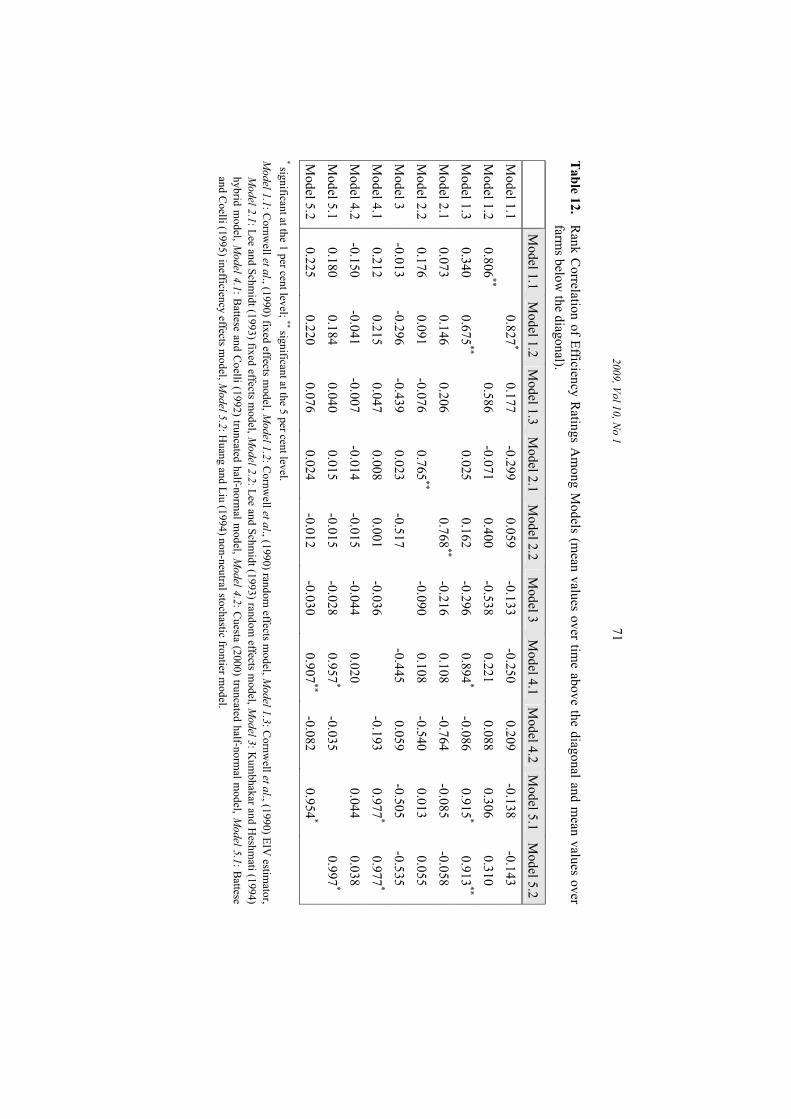
The Spearman’s correlation coefficients reported in Table 12 confirm the above find-ings. All the CSS models (1.1 through 1.3) exhibit high and statistically significant cor-relation coefficients of the mean technical efficiency ratings over farms and time. The

68

AGRICU

LTUR

AL ECO

+OMICS REVIEW

Tabl

e 9.

Produ

ction

Elast

icitie

s, Retu

rns to

Scale

and R

ate of

Tech

nical

Chan

ge

Mo

del 1

.1 Mo

del 1

.2 Mo

del 1

.3 Mo

del 2

.1 Mo

del 2

.2 Mo

del 4

.1 Mo

del 4

.2 Mo

del 5

.1 Mo

del 5

.2 Pro

ducti

on El

astici

ties

Labo

r 0.3

163

0.333

7 0.2

739

0.301

0 0.3

718

0.303

4 0.4

735

0.300

4 0.2

902

Fertil

izers

0.058

2 0.0

767

0.135

9 0.1

459

0.115

6 0.1

309

0.056

4 0.0

958

0.122

5 Ot

her

0.133

2 0.1

760

0.134

6 0.2

036

0.212

0 0.2

271

0.113

6 0.2

290

0.219

1 Ar

ea 0.4

478

0.406

8 0.4

211

0.459

2 0.3

815

0.329

4 0.4

195

0.324

4 0.3

449

RTS

0.955

5 0.9

932

0.965

6 1.1

096

1.081

0 0.9

908

1.063

0 0.9

497

0.976

8 Te

chnic

al Ch

ange

To

tal

2.845

3 3.0

928

3.454

6 2.0

705

1.199

0 2.6

611

2.227

1 2.2

532

1.102

3 Ne

utral

2.771

4 2.0

322

3.483

2 1.8

659

0.519

8 0.7

154

2.200

2 0.4

538

0.458

3 Bi

ased

0.074

0 1.0

606

-0.02

85

0.204

6 0.6

792

1.945

7 0.0

269

1.799

4 0.6

440

Model 1.1:

Cornw

ell et

al.,

(1990

) fixe

d effe

cts m

odel,

Mod

el 1.2:

Cornw

ell et

al.,

(1990

) ran

dom

effect

s mod

el, M

odel

1.3:

Cornw

ell et

al.,

(1990

) EIV

estim

ator,

Mod

el 2.1:

Lee a

nd Sc

hmidt

(199

3) fix

ed ef

fects

mode

l, Mod

el 2.2:

Lee a

nd Sc

hmidt

(199

3) ran

dom

effect

s mod

el, M

odel

4.1:

Batte

se an

d Coe

lli (19

92) tr

un-

cated

half-

norm

al mo

del, M

odel

4.2:

Cuest

a (20

00) tr

uncat

ed ha

lf-no

rmal

mode

l, Mod

el 5.1:

Batte

se an

d Coe

lli (19

95) in

effici

ency

effec

ts mo

del, M

odel

5.2:

Huan

g and

Liu (

1994

) non

-neutr

al sto

chast

ic fro

ntier

mode

l.

2009, Vol 10, )o 1 69

Table 10. Mean Technical Efficiency Ratings over Time 1987 1988 1989 1990 1991 1992 1993 Av/ge Model 1.1 69.00 67.91 75.38 80.27 75.30 69.19 60.64 71.10 Model 1.2 65.91 69.29 71.86 77.94 78.23 73.95 65.23 71.77 Model 1.3 51.62 53.84 57.08 60.14 59.56 61.66 59.62 57.64 Model 2.1 68.14 63.23 58.68 62.80 65.06 69.68 63.58 64.45 Model 2.2 65.14 65.03 60.51 62.89 68.70 68.90 61.33 64.64 Model 3 63.55 62.43 62.72 63.00 60.77 62.44 62.58 62.50 Model 4.1 74.33 75.28 76.20 77.10 77.97 78.81 79.63 77.05 Model 4.2 85.99 89.98 88.66 89.12 86.90 86.18 87.77 87.80 Model 5.1 83.63 85.05 86.16 86.52 87.20 87.47 88.30 86.33 Model 5.2 76.07 77.44 78.72 78.82 79.85 80.13 80.79 78.83

Model 1.1: Cornwell et al., (1990) fixed effects model, Model 1.2: Cornwell et al., (1990) random effects model Model 1.3: Cornwell et al., (1990) EIV estimator, Model 2.1: Lee and Schmidt (1993) fixed ef-fects model, Model 2.2: Lee and Schmidt (1993) random effects model, Model 3: Kumbhakar and Heshmati (1994) hybrid model, Model 4.1: Battese and Coelli (1992) truncated half-normal model, Model 4.2: Cuesta (2000) truncated half-normal model, Model 5.1: Battese and Coelli (1995) ineffi-ciency effects model, Model 5.2: Huang and Liu (1994) non-neutral stochastic frontier model.

Table 11. Frequency Distribution of Mean Technical Efficiency Ratings over Farms and Time

% Model 1.1

Model 1.2

Model 1.3

Model 2.1

Model 2.2

Model 3

Model 4.1

Model 4.2

Model 5.1

Model 5.2

<40 0 0 0 0 0 0 1 0 0 0 40-50 0 0 0 0 19 2 3 0 0 0 50-60 0 0 35 32 47 30 10 0 0 3 60-70 49 45 44 46 27 59 12 5 3 7 70-80 43 43 16 21 5 9 23 9 12 36 80-90 8 12 5 1 2 0 42 63 46 54 >90 0 0 0 0 0 0 9 23 39 0

Mean 71.10 71.77 57.64 57.3 64.64 62.50 77.05 87.80 86.33 78.83 Min 61.23 62.03 46.25 51.2 58.39 48.62 39.43 62.68 62.59 50.15 Max 85.13 88.36 87.70 78.9 83.40 75.99 94.44 91.29 96.35 88.13

Model 1.1: Cornwell et al., (1990) fixed effects model, Model 1.2: Cornwell et al., (1990) random effects model Model 1.3: Cornwell et al., (1990) EIV estimator, Model 2.1: Lee and Schmidt (1993) fixed ef-fects model, Model 2.2: Lee and Schmidt (1993) random effects model, Model 3: Kumbhakar and Heshmati (1994) hybrid model, Model 4.1: Battese and Coelli (1992) truncated half-normal model, Model 4.2: Cuesta (2000) truncated half-normal model, Model 5.1: Battese and Coelli (1995) ineffi-ciency effects model, Model 5.2: Huang and Liu (1994) non-neutral stochastic frontier model.


0

10

20

30

40

50

60

70

20-30 30-40 40-50 50-60 60-70 70-80 80-90 90-100Year

Effici

ency

(%)

Model 1.1Model 1.2Model 1.3Model 2.1Model 2.2Model 3Model 4.1Model 4.2Model 5.1Model 5.2

Figure 1. Frequency Distribution of Mean Technical Efficiencies (average values of the 1987-

93 period)

30

40

50

60

70

80

90

100

1987 1988 1989 1990 1991 1992 1993

Year

Effici

ency

(%)

Model 1.1 Model 1.2 Model 1.3 Model 2.1Model 2.2 Model 3 Model 4.1 Model 4.2Model 5.1 Model 5.2

Figure 2. Time Development of Efficiency Ratings same is true for both LS models (2.1 and 2.2). On the other hand, Models 4.1, 5.1 and 5.2 seems to exhibit very close point estimates of mean technical efficiencies over farms and time.

2009, Vol 10, )o 1

71

Table 12. Rank Correlation of Efficiency Ratings Among Models (mean values over time above the diagonal and mean values over farms below the diagonal).

Model 1.1 Model 1.2 Model 1.3 Model 2.1 Model 2.2

Model 3 Model 4.1 Model 4.2 Model 5.1 Model 5.2

Model 1.1

0.827*

0.177 -0.299

0.059 -0.133

-0.250 0.209

-0.138 -0.143

Model 1.2 0.806

**

0.586 -0.071

0.400 -0.538

0.221 0.088

0.306 0.310

Model 1.3 0.340

0.675**

0.025

0.162 -0.296

0.894*

-0.086 0.915

* 0.913

**

Model 2.1 0.073

0.146 0.206

0.768

** -0.216

0.108 -0.764

-0.085 -0.058

Model 2.2 0.176

0.091 -0.076

0.765**

-0.090

0.108 -0.540

0.013 0.055

Model 3 -0.013

-0.296 -0.439

0.023 -0.517

-0.445

0.059 -0.505

-0.535 Model 4.1

0.212 0.215

0.047 0.008

0.001 -0.036

-0.193

0.977*

0.977*

Model 4.2 -0.150

-0.041 -0.007

-0.014 -0.015

-0.044 0.020

0.044

0.038 Model 5.1

0.180 0.184

0.040 0.015

-0.015 -0.028

0.957*

-0.035

0.997*

Model 5.2 0.225

0.220 0.076

0.024 -0.012

-0.030 0.907

** -0.082

0.954*

* significant at the 1 per cent level; ** significant at the 5 per cent level. Model 1.1: Cornwell et al., (1990) fixed effects model, Model 1.2: Cornwell et al., (1990) random effects model, Model 1.3: Cornwell et al., (1990) EIV estimator,

Model 2.1: Lee and Schmidt (1993) fixed effects model, Model 2.2: Lee and Schmidt (1993) random effects model, Model 3: Kumbhakar and Heshmati (1994) hybrid model, Model 4.1: Battese and Coelli (1992) truncated half-normal model, Model 4.2: Cuesta (2000) truncated half-normal model, Model 5.1: Battese and Coelli (1995) inefficiency effects model, Model 5.2: Huang and Liu (1994) non-neutral stochastic frontier model.


Table 13. Ranking of Farms According to Technical Efficiency Estimates Obtained from Model 1.1

Model 1.1

Model 1.2

Model 1.3

Model 2.1

Model 2.2

Model 3

Model 4.1

Model 4.2

Model 5.1

Model 5.2

Most Efficient Farms 1 10 91 95 70 83 66 12 67 54 2 11 25 62 25 34 99 14 99 100 3 2 93 61 33 4 98 43 98 99 4 14 36 85 95 40 97 98 94 91 5 4 81 18 50 48 94 18 91 92 6 5 72 25 37 56 90 22 93 93 7 3 82 47 48 60 87 7 87 88 8 7 44 12 29 95 96 76 95 95 9 6 77 74 55 1 59 49 64 72

10 13 66 87 40 10 81 44 77 81 11 12 96 48 45 93 51 96 42 52 12 15 50 14 68 99 40 87 50 61 13 16 76 16 24 67 16 83 32 22 14 17 52 55 22 21 28 69 21 6 15 9 97 98 65 13 74 90 59 62

Least Efficient Farms 86 98 5 86 67 70 25 3 44 53 87 82 37 79 39 100 5 45 13 3 88 93 26 22 23 24 15 36 25 41 89 84 14 89 18 87 38 51 48 36 90 89 27 73 21 86 43 92 38 42 91 96 6 1 1 26 41 82 43 47 92 95 4 68 26 94 79 38 82 83 93 88 41 58 6 96 93 35 96 89 94 87 23 82 19 73 84 40 84 94 95 94 1 83 10 8 26 25 30 8 96 97 2 76 30 65 4 11 23 17 97 63 19 93 2 45 64 21 57 34 98 99 11 84 17 78 1 8 1 2 99 71 86 41 32 14 85 26 85 78

100 100 15 77 14 32 76 42 78 74 Model 1.1: Cornwell et al., (1990) fixed effects model, Model 1.2: Cornwell et al., (1990) random effects

model, Model 1.3: Cornwell et al., (1990) EIV estimator, Model 2.1: Lee and Schmidt (1993) fixed ef-fects model, Model 2.2: Lee and Schmidt (1993) random effects model, Model 3: Kumbhakar and Heshmati (1994) hybrid model, Model 4.1: Battese and Coelli (1992) truncated half-normal model, Model 4.2: Cuesta (2000) truncated half-normal model, Model 5.1: Battese and Coelli (1995) ineffi-ciency effects model, Model 5.2: Huang and Liu (1994) non-neutral stochastic frontier model.

2009, Vol 10, +o 1 73

However, Cuesta’s (2000) formulation (Model 4.2) results to considerably different mean values. It is noteworthy the fact that the temporal patterns of mean technical effi-ciency obtained from Model 1.3 is similar to that resulted from Models 5.1 (BC95) and 5.2 (HL) as that is indicated from the high and statistical significant Spearman correla-tion coefficients.

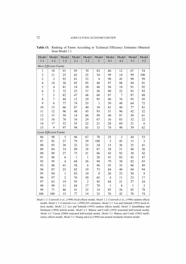
Besides the differences in the frequency distribution and the temporal patterns of mean technical efficiencies, alternative model specifications reveal significant different of individual rankings of the surveyed farms. Table 13 shows the discrepancy in the efficiency rankings of (the same) 15 farms under the different model specifications of the production frontier. As it is evident from this table we can observe a relative con-cordance between Models 1.1 and 1.2, between Models 2.1 and 2.2 and between Models 5.1 and 5.2. However, it is noteworthy the fact that besides CSS EIV estimator (Model 1.3) results to high and statistical significant correlation coefficients with the other two CSS estimators (Models 1.1 and 1.2) the relevant ranking of mean technical efficiency ratings is considerably different.

Selection of the Stochastic Frontier Model The empirical results presented in the previous section show that different model

specification of the stochastic production frontier and the temporal patterns of technical inefficiency result in different conclusions concerning the individual performance in the use of the available resources. Since the empirical results are model specific, the ques-tion that naturally arises is what the model specification that fits the data best. However, not all the alternative models are nested to each other and therefore it is not always pos-sible to statistically discriminate among them.

Table 14 presented nested hypothesis testing between the alternative model specifi-cation. First, the Hausman specification test of the CSS-LSDV estimator (Model 1.1) against CSS-GLS estimator (Model 1.2) gives a chi-square statistic of 22.7 lower than the corresponding critical value at the 5% level of significance. Further, testing Model 1.2 against Model 1.3 we find that the later is the preferred choice among all CSS mod-els implying that only some of the regressors are uncorrelated with the individual ef-fects.29 On the other hand, when testing Model 2.1 against Model 2.2, Hausman specifi-

Table 14. Nested Hypotheses Testing for the Alternative Model Specifications Hypothesis Test-statistic Critical Value 1. Model 1.1 vs Model 1.2 22.7 2

20 31.4χ = 2. Model 1.3 vs Model 1.2 12.5 2

10 18.3χ = 3. Model 2.1 vs Model 2.2 25.3 2

20 31.4χ = 4. Model 4.1 vs Model 4.21 243.9 2

100 124χ ≈ 5. Model 5.1 vs Model 5.21 28.6 2

8 15.5χ = 1 The corresponding restrictions are iη θ= and 0mjδ = m∀ , respectively.


cation test indicates again that the LS-GLS (Model 2.2) estimator is the appropriate choice.

Concerning the ML estimators the LR-test indicates that Models 4.2 and 5.2 outper-form Models 4.1 and 5.1 respectively. Specifically, the hypothesis that ηi=θ ∀i is re-jected at the 5% level of significance indicating that CT model cannot be reduced to BC92 specification. On the other hand, the hypothesis that the interaction terms of pro-ducer-specific characteristics with the input variables in the inefficiency effects are zero (δmj=0 ∀m) is also rejected suggesting that HL generalization of BC95 model specifica-tion is more appropriate.

So from the ten alternative frontier specification only 5 of them are statistically ac-ceptable in modeling individual technical efficiency in our data set. Unfortunately, it is not possible to further narrow down the alternatives as they are not nested to each other. The statistically inability to determine the appropriate specification is bothersome given that the resulted five models reveal different conclusions concerning the production possibilities of Greek olive-growing farms and the efficiency in the use of their re-sources.

Certainly, the inability to achieve the “first best” should not be perceived as an anathema to specification searches. Since it is evident from our comparative analysis that individual technical efficiency estimates are indeed sensitive to the choice of the model of pooling, one should always attempt to statistically discriminate among the vi-able alternatives. Despite the drawbacks in our case statistical testing did narrow down the set of suitable alternative from ten to five specifications.

The natural question that arises is then what is the best way to proceed in cases where it is not statistically feasible to find the appropriate specification. As suggested by Coelli and Perelman (1999), a potential solution can be borrowed from time-series fore-casting literature where many authors suggest that composite predictions quite often outperform any particular predictive model. Palm and Zellner (1992, p. 699) argue that “in many cases a simple average of forecasts achieves a substantial reduction in vari-ance and bias”. Based on this suggestion, when it is not possible to distinguish among different model specifications which provide different predictions of individual techni-cal efficiency, a composite measure can provide a solution for reducing the bias of the obtained efficiency estimates.

Coelli and Perelman (1999) argue that in cases where there is no a priori reason for choosing among different model specifications, one should construct geometric means of the obtained technical efficiency estimates at each data point. Following their sugges-tion we proceed to the construction of the geometric means of individual technical effi-ciency ratings obtained from Models 1.3, 2.2, 4.2 and 5.2. The results are presented in Table 15 in the form of frequency distribution within a decile range.

According to these estimates mean technical efficiency over farms and time is 68.45% following a slightly increase through time. The lowest value is observed in 1987, 66.42% and the highest in 1992, (70.33%).

Concluding remarks Several alternative models for the estimation of technical efficiency in the context of

panel data were reviewed and estimated. These estimates were obtained by using a ran-

2009, Vol 10, +o 1 75

Table 15. Frequency Distribution of Technical Efficiency Ratings Obtained as the Geometric Mean of Models 1.3, 2.2, 4.2 and 5.2

% 1987 1988 1989 1990 1991 1992 1993 <20 0 0 0 0 0 0 0

20-30 0 0 0 0 0 0 0 30-40 0 0 0 0 0 0 0 40-50 0 0 0 0 0 0 0 50-60 15 7 9 3 2 5 1 60-70 57 58 59 57 51 43 53 70-80 28 35 29 40 46 49 45 80-90 0 0 3 0 1 3 1 >90 0 0 0 0 0 0 0

Mean 66.42 67.56 67.63 69.09 69.55 70.33 68.55 Min 51.61 53.30 56.06 56.48 56.44 54.71 58.33 Max 79.81 78.88 85.16 78.63 86.54 83.73 80.45

dom sample consisting of 100 olive-growing farms in Greece during the 1987-93 pe-riod. The empirical results indicate that although the alternative models reveal minor differences concerning the production structure of the olive-growing farms in the sam-ple, the estimates of technical efficiency obtained from these models differ considerably among them. Specifically, mean technical efficiency was found to range by almost 30% across models which underlines the significance of the choice for the model of pooling.

It should be noted here that these findings are rather data specific and there is no a priori reason for expecting any particular study to exhibit the same pattern in the final efficiency estimates. On the other hand, there is no any economic or theoretical basis for choosing any particular model for the estimation of technical efficiency. Each model has advantages as well as certain shortcomings relative to the other. However, empiri-cally the efficiency measures derived in each particular case study are important from a policy point of view. Since there is no a priori reason for choosing any of the alternative models proposed in the literature, one must be very careful on his choice particularly when important policy measures are to be derived from that specific study. 7otes 1 Adding more observations on each production unit generates information not pro-

vided by simply adding more producers to a cross-section data set (Schmidt and Sickles, 1984).

2 In addition, the availability of panel data resolves the inconsistency of Jondrow et al., (1982) predictor of individual technical efficiencies.

3 As noted by Greene (1990), an inappropriate statistical distribution besides is not affecting both rankings or decile decompositions of technical efficiency estimates, it is indeed affecting mean individual efficiencies.


4 However, whenever this is not possible, repeated observations on production units can serve as a substitute for the independence assumption (Kumbhakar and Lovell, 2000, p. 96).

5 Kumbhakar (2000) summarizes the theoretical framework for decomposing total fac-tor productivity based on either a primal or a dual frontier model in the context of panel data.

6 Maximum likelihood models are not in general nested to each other. Battese and Coelli’s (1992) model specification is nested to that of Cuesta (2000) but not to that of Huang and Liu (1994) or to that of Battese and Coelli (1995). On the other hand, while random and fixed effects models can be statistically discriminated by means of LaGrange multiplier (LM) test, the same is not feasible for the various specifications of time-varying technical efficiency. Lee and Schmidt (1993) model specification nests that of Kumbhakar (1990) but not that of Cornwell et al., (1990).

7 In this case individual specific intercepts (β0i) are recovered using the means over time of the obtained residuals.

8 Alternatively, as noted by Kumbhakar and Lovell (2000, p. 109), this restriction can be interpreted as the time-invariant technical inefficiency where the quadratic term captures the rate of technical change. It is not possible to distinguish between these effects.

9 This means that in each period at least one producer is fully efficient, although the identity of this producer may vary through years.

10 LS noted that the choice of normalization has no substantive implications. 11 Another way of viewing the distinction between the fixed and random effects models

is as a distinction between conditional and unconditional inference. The former seems appropriate when we are particularly interested in those individuals in the sample, while the later is appropriate if we are interested in inferences about the population of which the data set arises.

12 If, however, T is large but < is small, only the within estimator is consistent. But still there is no consistent way of separating firm efficiency from white noise (Schmidt and Sickles, 1984). Hence, efficiency is compared across firms and not relative to an absolute standard.

13 Persistent technical inefficiency is closely related to government policy and firm-ownership, while the residual time-varying technical inefficiency is due to temporary factors (Kumbhakar and Heshmati, 1995). In the extreme case of 0iµ = , technical inefficiency varies randomly across firms as well as over time.

14 This may be case with changes in governmental policy. Lovell (1996) also raised the concern of whether is possible to distinguish the effect of firm-specific persistent technical inefficiency from that of quasi-fixed inputs, which also vary across firms but not through time.

15 In the case of unbalanced panels, t includes a subset of integers representing the peri-ods for which observations on individual producers are obtained.

16 Battese and Coelli (1992) provide in the appendix the corresponding likelihood func-tion as well as the conditional expectation of uit.

2009, Vol 10, +o 1 77

17 Biased estimates of mδ parameters may be obtained by not including an intercept parameter 0δ in the mean, iµ , since in such a case the shape of the distribution of the inefficiency effects is unnecessarily restricted (Battese and Coelli, 1995).

18 Battese and Coelli (1993) provide the relevant likelihood function as well as the con-ditional expectation of uit.

19 The two-stage approach for identifying factors influencing technical inefficiencies suggested by Timmer (1971) suffers from two important econometric problems (Kumbhakar and Lovell, 2000, p. 264): first, it is presumed that X and z are corre-lated in the second-stage regression. However, in this case ML estimates of the fron-tier model are biased due to the omission of z variables which in turn implies that technical efficiencies used in the second-stage regression are biased estimates of their true values. Second, it is assumed in the first-stage that individual technical efficien-cies are identically distributed, but this assumption is violated in the second-stage re-gression as predicted efficiencies are assumed to have a functional relationship with z variables.

20 Reifschneider and Stevenson (1991) suggested but not implemented a model in which the variance is a function of the z-vector. Mester (1993) and Yuengert (1993) provided a very simple version of this suggestion.

21 All variables are expressed in their natural logarithms. 22 All relevant parameter restrictions for hypotheses testing presented in Table 4 are

given in Chung (1994, pp. 139-154). 23 The F-test is computed as ( ) ( )

( )1r u

u

RSS RSS "F

RSS "T " k− −

=− −

where, RSSr and RSSu are the

residual sum of squares from the restricted and unrestricted models, respectively. 24 If 2 0uσ = then the least squares estimator is best linear unbiased and farm-effects are

zero (Breusch and Pagan, 1980). The LM-test statistic is computed by

( )22

2 12 1

T T

it iti t i t

Tλ ε εT

= − − ∑ ∑ ∑∑

and it is asymptotically distributed as chi-squared with one degree of freedom. 25 The LR-test statistic is calculated as ( ) ( )*2 ln lnLR L θ L θ = − where * denotes

estimates from the unrestricted model. 26 Recall that it is not possible to statistical test the temporal pattern of technical ineffi-

ciency in KH model specification. 27 Since in Model 5.2 conventional inputs also appear in the inefficiency effects model,

the corresponding point elasticity estimates were computed using the formulas set forth by Huang and Liu (1994) and Battese and Broca (1997).

28 Technical change is input using, neutral or saving as αj is greater, equal or less than zero, respectively.

29 The Hausman-test in this case can be interpreted as a test that all the regressors are uncorrelated with the individual effects (Model 1.2) against the alternative that only


some of them are uncorrelated (Model 1.3). In this case the degrees of freedom of the χ2-test equals with the rank of the difference between the variance-covariance matri-ces of the estimators compared (GLS and EIV). In our case, the EIV estimator was obtained assuming that ten out of twenty of the explanatory variables were uncorre-lated with the individual effects. Our choice was based on the correlation between individual effects obtained from the GLS estimator and the independent variables (Hallam and Machado, 1996).

References Aigner, D.J., C.A.K. Lovell and P. Schmidt (1977). “Formulation and Estimation of Stochastic

Frontier Production Function Models.” Journal of Econometrics 6, 21-37. Baltagi, B.H. and J.M. Griffin (1988). “A General Index of Technical Change.” Journal of Po-

litical Economy 96, 20-41. Battese, G.E. and T.J. Coelli (1988). “Prediction of Firm-Level Technical Efficiencies with

Generalized Frontier Production Function and Panel Data.” Journal of Econometrics 38, 387-399.

Battese, G.E. and T.J. Coelli (1992). “Frontier Production Functions, Technical Efficiency and Panel Data: With Application to Paddy Farmers in India.” Journal of Productivity Analy-sis 3, 153-169.

Battese, G.E. and T.J. Coelli (1993). “A Stochastic Frontier Production Function Incorporating a Model for Technical Inefficiency Effects.” Working Paper in Econometrics and Applied Statistics No 69, Department of Econometrics, University of New England, Armidale, Australia.

Battese, G.E. and T.J. Coelli (1995). “A Model for Technical Inefficiency Effects in a Stochas-tic Frontier Production Function for Panel Data.” Empirical Economics 20, 325-332.

Breusch, T.S. and A.R. Pagan (1980). “The LaGrange Multiplier Test and its Applications to Model Specification in Econometrics.” Review of Economic Studies 47, 239-254.

Breusch, T.S., G.E. Mizon and P. Schmidt (1989). “Efficient Estimation Using Panel Data.” Econometrica 57, 695-700.

Chung, J.W. (1994). “Utility and Production Functions.” Cambridge MA: Backwell. Coelli, T.J. (1995). “A Monte Carlo Analysis of the Stochastic Frontier Production Function.”

Journal of Productivity Analysis 6, 247-268. Cornwell, C., P. Schmidt and R.C. Sickles (1990). “ Production Frontiers with Cross-Sectional

and Time-Series Variation in Efficiency Levels.” Journal of Econometrics 46, 185-200. Cuesta, R.A. (2000). “A Production Model with Firm-Specific Temporal Variation in Technical

Inefficiency: With Application to Spanish Dairy Farms.” Journal of Productivity Analysis 13, 139-158.

Greene, W.H. (1990). “A Gamma-Distributed Stochastic Frontier Model.” Journal of Econo-metrics 46, 141-163.

Greene, W.H. (1993). “Econometric Analysis.” New York: Prentice Hall Inc. Hallam, D. and F. Machado (1996). “Efficiency Analysis with Panel Data: A Study of Portu-

guese Dairy Farms.” European Review of Agricultural Economics 23, 79-93. Huang, C.J. and J.T. Liu (1994). “Estimation of a Non-Neutral Stochastic Frontier Production

Function.” Journal of Productivity Analysis 5, 171-180.

2009, Vol 10, +o 1 79

Jondrow, J., C.A.K. Lovell, I.S. Materov and P. Schmidt (1982). “On the Estimation of Techni-cal Inefficiency in the Stochastic Frontier Production Function Model.” Journal of Econometrics 19, 233-238.

Kodde, D.A. and F.C. Palm (1986). “Wald Criteria for Jointly Testing Equality and Inequality Restrictions.” Econometrica 54, 1243-48.

Kumbhakar, S.C. (2000). “Estimation and Decomposition of Productivity Change when Produc-tion is not Efficient: A Panel Data Approach.” Econometric Reviews

Kumbhakar, S.C. and A. Heshmati (1995). “Efficiency Measurement in Swedish Dairy Farms: An Application of Rotating Panel Data, 1976-1988.” American Journal of Agricultural Economics 77, 660-674.

Kumbhakar, S.C. and C.A.K. Lovell (2000). “Stochastic Frontier Analysis.” Cambridge: Cam-bridge University Press.

Kumbhakar, S.C., A. Heshmati and L. Hjalmarsson (1997). “Temporal Patterns of technical Efficiency: Results from Competing Models.” International Journal of Industrial Or-ganization 15, 597-616..

Kumbhakar, S.C., S. Ghosh and J.T. McGuckin (1991). “A Generalized Production Frontier Approach for Estimating Determinants of Inefficiency in U.S. Dairy Farms.” Journal of Business and Economic Statistics 9, 279-86.

Lee, Y.H. and P. Schmidt (1993). “A Production Frontier Model with Flexible Temporal Varia-tion in Technical Efficiency.” in H.O. Fried, C.A.K. Lovell and P. Schmidt (eds.), The Measurement of Productive Efficiency: Techniques and Applications, New York: Oxford University Press.

Lovell, C.A.K. (1996). “Applying Efficiency Measurement Techniques to the Measurement of Productivity Change.” Journal of Productivity Analysis 7, 329-40.

Mester, L.J. (1993). “Efficiency in the Savings and Loan Industry.” Journal of Banking and Finance 17(2/3), 267-286.

Pitt, M.M. an L.F. Lee (1981). “The Measurement and Sources of Technical Inefficiency in the Indonesian Weaving Industry.” Journal of Development Economics 9, 43-64.

Reifschneider, D. and R. Stevenson (1991). “Systematic Departures from the Frontier: A Framework for the Analysis of Firm Inefficiency.” International Economic Review 32, 715-723.

Schmidt, P. and R.C. Sickles (1984). “Production Frontiers and Panel Data.” Journal of Busi-ness and Economic Statistics 2, 367-374.

Stevenson, R.E. (1980). “Likelihood Functions for Generalized Stochastic Frontier Estimation.” Journal of Econometrics 13, 58-66.

Timmer, C.P. (1971). “Using a Probabilistic Frontier Production Function to Measure Technical Efficiency.” Journal of Political Economy 79, 776-794.

Yuengert, A.W. (1993). “The Measurement of Efficiency in Life Insurance: Estimates of a Mixed Normal-Gamma Error Model.” Journal of Banking and Finance 17(2/3), 401-405.

parametric measurement of time-varying technical...

Documents