Parameter estimation of a physically based land surface hydrologicmodel using the ensemble Kalman filter: A synthetic experiment

Yuning Shi,1 Kenneth J. Davis,1 Fuqing Zhang,1 Christopher J. Duffy,2 and Xuan Yu2

Received 3 May 2013; revised 1 December 2013; accepted 17 December 2013; published 29 January 2014.

[1] This paper presents multiple parameter estimation using multivariate observations viathe ensemble Kalman filter (EnKF) for a physically based land surface hydrologic model. Adata assimilation system is developed for a coupled physically based land surfacehydrologic model (Flux-PIHM) by incorporating EnKF for model parameter and stateestimation. Synthetic data experiments are performed at a first-order watershed, the ShaleHills watershed (0.08 km2). Six model parameters are estimated. Observations of discharge,water table depth, soil moisture, land surface temperature, sensible and latent heat fluxes,and transpiration are assimilated into the system. The results show that, given a limitednumber of site-specific observations, the EnKF can be used to estimate Flux-PIHM modelparameters. All the estimated parameter values are very close to their true values, with thetrue values inside the estimated uncertainty range (1 standard deviation spread). Theestimated parameter values are not affected by the initial guesses. It is found that discharge,soil moisture, and land surface temperature (or sensible and latent heat fluxes) are the mostcritical observations for the estimation of those six model parameters. The assimilation ofmultivariate observations applies strong constraints to parameter estimation, and providesunique parameter solutions. Model results reveal strong interaction between the vanGenuchten parameters a and b, and between land surface and subsurface parameters. TheEnKF data assimilation system provides a new approach for physically based hydrologicmodel calibration using multivariate observations. It can be used to provide guidance forobservational system designs, and is promising for real-time probabilistic flood and droughtforecasting.

Citation: Shi, Y., K. J. Davis, F. Zhang, C. J. Duffy, and X. Yu (2014), Parameter estimation of a physically based land surface hydrologicmodel using the ensemble Kalman filter: A synthetic experiment, Water Resour. Res., 50, 706–724, doi:10.1002/2013WR014070.

1. Introduction

[2] Land surface models (LSMs) and hydrologic modelsare important tools for the forecasting and study of landsurface and hydrologic processes. LSMs simulate theexchange of mass, momentum and energy between the landsurface and the atmosphere. They play important roles inweather and climate forecasting, and provide necessarylower boundary conditions for atmospheric models. Hydro-logic models simulate hydrologic system responses toincoming precipitation. They are essential for predictingflood and drought events and are routinely used for deci-sions that have considerable societal impacts. Both LSMsand hydrologic models are highly parameterized. Modelstructures are complex and the number of involved parame-

ters is often large. The accuracy of LSMs and hydrologicmodels is limited by, among other factors, the uncertaintiesin model parameters. Parameter estimation of LSMs andhydrologic models has been the focus of many studies[e.g., Gupta et al., 1999; Xia et al., 2002; Jackson et al.,2003].

[3] Uncertainties in model parameters are an especiallydominant source of uncertainty for hydrologic models[Moradkhani and Sorooshian, 2008]. Hydrologic modelparameters nearly always require calibration for specificwatersheds before they can produce realistic responses toenvironmental inputs such as precipitation. For hydrologicmodels, the physical parameter values in actual field condi-tions might be substantially different from those measuredin laboratory; the range of variation in parameter valuesspans orders of magnitude [Bras, 1990]. Some physicalparameters may be heterogeneous in space, which compli-cates the task of obtaining accurate parameter estimates.Consequently, model calibration is one of the mostdemanding and time-consuming tasks in applying hydro-logic models, and the resulting parameter values often haveconsiderable uncertainty even after optimization.

[4] In the past few decades, many hydrologic model cali-bration methods have been proposed and studied. A basiccalibration approach is the trial and error method, i.e.,

1Department of Meteorology, Pennsylvania State University, UniversityPark, Pennsylvania, USA.

2Department of Civil Engineering, Pennsylvania State University, Uni-versity Park, Pennsylvania, USA.

Corresponding author: Y. Shi, Department of Meteorology, Pennsylva-nia State University, 415 Walker Bldg., University Park, PA 16802, USA.(yshi@psu.edu)

©2013. American Geophysical Union. All Rights Reserved.0043-1397/14/10.1002/2013WR014070

706

WATER RESOURCES RESEARCH, VOL. 50, 706–724, doi:10.1002/2013WR014070, 2014

manual calibration. In manual calibration, model perform-ances are visually inspected, and then model parameter val-ues are tuned to minimize the differences between modelpredictions and observations, based on human judgment[Boyle et al., 2000; Moradkhani and Sorooshian, 2008].This method is very labor intensive and time consuming.Manual calibration of physically based hydrologic modelscan be extremely difficult due to the high dimensionality ofthe parameter space and the strong interaction betweenmodel parameters. It is also important to note that manualcalibration does not lead to a rigorous (if any) quantifica-tion of parameter uncertainty. Those difficulties motivatedthe development of automatic calibration methods.

[5] Generally, there are two strategies for automatic cali-bration: batch (iterative) calibration and sequential (recur-sive) calibration. Batch calibration aims to minimize thepredefined objective functions by repeatedly searching inthe parameter space and evaluating long period model per-formances [e.g., Ibbitt, 1970; Johnston and Pilgrim, 1976;Pickup, 1977; Gupta and Sorooshian, 1985; Duan et al.,1992; Sorooshian et al., 1993; Franchini, 1996; Wageneret al., 2003; Kollat and Reed, 2006; Yu et al., 2013]. Batchcalibration requires previously collected historical data formodel evaluation and is thus restricted to offline applica-tions. Batch calibration has limited flexibility in dealingwith the possible temporal evolution of model parameters[Moradkhani et al., 2005a; Moradkhani and Sorooshian,2008].

[6] Sequential calibration (data assimilation) methodscan take advantage of measurements whenever they areavailable and are thus useful in both online and offlineapplications. They have more flexibility in dealing withtime-variant parameters, compared with batch calibrationmethods. Some sequential calibration methods also explic-itly address uncertainties in input data and model struc-tures. Frequently used data assimilation methods for LSMsand hydrologic models include variational methods [e.g.,Reichle et al., 2002a; Lee et al., 2011], the particle filter[e.g., Moradkhani et al., 2005b; Weerts and El Serafy,2006; Salamon and Feyen, 2009], and different forms ofKalman filter, especially the ensemble Kalman filter[EnKF; e.g., Reichle et al., 2002a, 2002b; Crow andWood, 2003; Francois et al., 2003; Moradkhani et al.,2005a; Pan and Wood, 2006; Vrugt et al., 2006; Clarket al., 2008; Kumar et al., 2008; Camporese et al., 2009a;Xie and Zhang, 2010; Cammalleri and Ciraolo, 2012; Hanet al., 2012; Flores et al., 2012; Hain et al., 2012]. Varia-tional methods depend on the development of adjoint mod-els. The application of variational methods to LSMs andhydrologic models is thus difficult, because adjoints ofLSMs and hydrologic models are not always available andare difficult to derive [Reichle et al., 2002a, 2002b; Moranet al., 2004; Vrugt et al., 2006; Salamon and Feyen, 2009].The particle filter [Arulampalam et al., 2002] has noassumptions on the form of the prior probability densityfunction (PDF) of the model states and the model errors. Itcan maintain the predicted spatial pattern of distributed var-iables, because the particle filter updates the weights of dif-ferent ensemble members, instead of directly updating thestate variables. However, the particle filter requires manymore ensemble members than EnKF to produce good esti-mates of model errors, and is thus more computationally

expensive [Weerts and El Serafy, 2006; Clark et al., 2008;Salamon and Feyen, 2009]. EnKF [Evensen, 1994] hasbeen widely used for parameter estimation in recent years.EnKF has a simple conceptual formulation, relative ease ofimplementation (no adjoint needed), and affordable compu-tational requirements [Evensen, 2003]. EnKF is not onlyuseful in improving state and parameter estimations, butcan also provide uncertainty estimations of variables andparameters. Compared with other forms of Kalman filters,EnKF is capable of handling strongly nonlinear dynamics,high dimensional state vectors, and to some degree non-Gaussian parameter and state probability distributions.

[7] Because of the high computational demands ofprocess-based and physically-based hydrologic models, itis very difficult to use batch methods for calibration [Tanget al., 2006]. Their high dimensional parameter space andhigh nonlinearity pose difficulties for sequential methodsas well. Currently manual calibration, i.e., trial and errorprocedure, is still the prevalent choice for physically basedhydrologic model calibration [e.g., Pisinaras et al., 2010;Leimer et al., 2011; Shi et al., 2011; Shih and Yeh, 2011;Dechmi et al., 2012; Yao et al., 2012; Shi et al., 2013a].The EnKF provides a promising approach for distributedphysically based hydrologic model auto calibration. Mor-adkhani et al. [2005a] applied EnKF to a lumped concep-tual rainfall runoff (R-R) model to estimate the values offive model parameters using real observations, and foundthat the obtained parameter set from EnKF was similar tothe results from batch calibration. The ensemble dischargeprediction also agreed well with observations. Xie andZhang [2010] applied EnKF to a spatially distributed con-ceptual hydrologic model to estimate a spatially distributedmodel parameter, which had different values in differenthydrologic response units (HRUs). In the synthetic dataexperiments, at most HRUs, the estimated values of theparameter were very close to the true values when dis-charge observations were assimilated. L€u et al. [2013]applied EnKF to a lumped conceptual R-R model andfound that using dual state-parameter estimation improvesmodel streamflow estimation compared to the test casewhich only used state estimation. There are also studiesimplementing EnKF in groundwater models to estimatemodel parameters such as hydraulic conductivities [e.g.,Chen and Zhang, 2006; Liu et al., 2008; Hendricks Frans-sen et al., 2011; Kurtz et al., 2012]. Although EnKF hasbeen proven effective for lumped and distributed concep-tual watershed models and some physically based ground-water models, the effectiveness of EnKF in parameterestimation for spatially distributed physically based water-shed models, or land surface hydrologic models is stilluntested.

[8] Data assimilation for fully coupled physically basedhydrologic models using EnKF is difficult. Compared withconceptual models, physically based spatially distributedmodels generally have more model parameters, moremodel grids, and more state variables at each grid. A rela-tively large number of model grids with more state varia-bles and model parameters results in a high dimensionaljoint vector of states and parameters, which makes theimplementation of EnKF difficult and increases the compu-tational cost. Physically based models require a long adjust-ment period or spin-up after observations are assimilated

SHI ET AL.: PARAMETER ESTIMATION USING ENKF

707

and model states are updated. In physically based models,model formulations and parameters define the equilibriumamong model state variables in the system. The equilibriumof the system does not only include the equilibriumbetween surface water, saturated water storage, and unsatu-rated water storage within a model grid, but also the equi-librium among different grids. The update of state variablesand parameters via EnKF can disrupt the equilibrium in thesystem [Pan and Wood, 2006] which requires a time periodfor adjustment. The equilibrium needs to be reestablishedthrough the exchange of water among different water com-ponents in a single water grid (e.g., infiltration, ground-water recharge, and root zone uptake), and through theexchange of water among different grids (e.g., horizontalgroundwater flow and surface flow). During this adjustmentor spin-up period, the covariance matrix between the modelpredictions and the joint vector of states and parameters iscontaminated by this spin-up effect. If the assimilationinterval is shorter than the adjustment period, the EnKFwill update the state variables and model parameters usinga contaminated covariance matrix, which will degrade theaccuracy of the EnKF analysis. A long assimilation inter-val, however, means fewer observations can be assimilated,which can affect model performances due to the lack ofobservations. Therefore, finding the optimal assimilationinterval is important.

[9] Identifying critical observations for model parameterestimation is important for model calibration, for enhancingthe understanding of the inverse problem of parameter esti-mation, and for the observational system design at experi-mental sites. Classically, only discharge data are used forR-R model data assimilation, while soil moisture and landsurface temperature data are used for LSMs [e.g., Houseret al., 1998; Crow and Wood, 2003; Pauwels and De Lan-noy, 2006; Pan and Wood, 2006; Clark et al., 2008]. Somerecent studies have assimilated multiple types of observa-tions (multivariate observations) into hydrologic models(see a review by Montzka et al. [2012]). It has been shownthat the assimilation of soil moisture in addition to dis-charge into R-R model improves the forecast of discharge[e.g., Oudin et al., 2003; Aubert et al., 2003; Francoiset al., 2003; Camporese et al., 2009a, 2009b; Bailey andBa�u, 2010; Lee et al., 2011], especially during flood events[Aubert et al., 2003]. Xie and Zhang [2010] also found thatin synthetic experiments, the assimilation of soil moisturein addition to discharge improves the estimation of modelparameters.

[10] This paper presents a demonstration of multipleparameter estimation for a coupled physically based landsurface hydrologic model (Flux-PIHM) using multivariateobservations via EnKF. The hydrologic land surface modelused in this study is Flux-PIHM [Shi et al., 2013a], whichis based on the Penn State Integrated Hydrologic Model(PIHM) [Qu, 2004; Qu and Duffy, 2007; Kumar, 2009]and the land surface scheme from the Noah LSM [Chenand Dudhia, 2001; Ek et al., 2003]. Six Flux-PIHM param-eters, including three hydrologic parameters and three landsurface parameters are estimated using EnKF. Syntheticexperiments are performed to test the accuracy of EnKF inmultiple parameter estimation and to find the optimal timeinterval for data assimilation. Synthetic observations ofdischarge, water table depth, soil moisture content, land

surface temperature, sensible and latent heat fluxes, andcanopy transpiration, and various subsets of those observa-tions are assimilated to identify the observations critical forparameter estimation. The model is implemented at theShale Hills watershed (0.08 km2) in central Pennsylvania,where the broad array of observations provides the possibil-ity for a future real-data test.

2. Development of the Flux-PIHM DataAssimilation System

2.1. Flux-PIHM

[11] Flux-PIHM [Shi et al., 2013a] is a coupled land sur-face hydrologic model. Flux-PIHM incorporates a land-surface scheme into the Penn State Integrated HydrologicModel (PIHM) [Qu, 2004; Qu and Duffy, 2007; Kumar,2009]. PIHM is a fully coupled, physically based, and spa-tially distributed hydrologic model. It simulates channelflow, 2-D overland flow, 1-D unsaturated flow, and 2-Dgroundwater flow (with dynamic coupling to the unsatu-rated zone) in a physically based and fully coupled scheme.The land surface scheme in Flux-PIHM is adapted from theNoah LSM [Chen and Dudhia, 2001; Ek et al., 2003]. Theland surface and hydrologic components are coupled byexchanging water table depth, infiltration rate, rechargerate, net precipitation rate, and evapotranspiration ratebetween the two model components. Because Flux-PIHMis based on a spatially distributed, physically based, andfully coupled hydrologic model, the computational cost isrelatively high. It has previously been manually calibratedand tested at the Shale Hills watershed (0.08 km2) [Shiet al., 2013a].

2.2. The Ensemble Kalman Filter

[12] After its introduction by Evensen [1994], EnKF hasbeen widely used in atmospheric, geographic, and oceanicsciences. It was first developed for dynamic state estima-tion to improve initial conditions for numerical forecasts,and was later applied to model parameter estimation.

[13] The EnKF formulation used by Snyder and Zhang[2003] is adopted in this study. In EnKF, the posterior esti-mate xa, i.e., the analysis is given by

xa5xf 1K y2Hxf� �

; (1a)

and the analysis error covariance Pa is given by

Pa5 I2KHð ÞPf ; (1b)

where xf is the prior estimate with n state variables, y is theobservation vector of m observations, H is the observationoperator matrix (dimension m 3 n) which maps state varia-bles to observations, I is an identity matrix (dimension n 3n), and Pf is the forecast background error covariance(dimension n 3 n). The Kalman gain matrix K (dimensionn 3 m) is defined as

K5Pf HT HPf HT1R� �21

; (2)

where R is the observation error covariance (dimensionm 3 m). Pf HT is the forecasted covariance between the

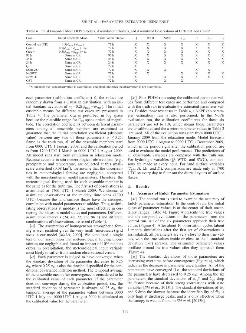
SHI ET AL.: PARAMETER ESTIMATION USING ENKF

708

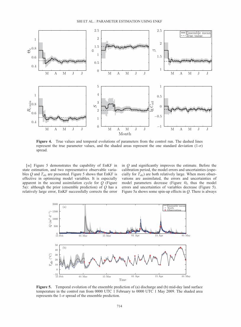
states and observed variables, and HPf HT is the forecastederror covariance of the observed variables.

[14] The state augmentation approach, which has beentested in many studies [e.g., Annan, 2005; Aksoy et al.,2006; Hu et al., 2010; Xie and Zhang, 2010], is adopted forparameter estimation. In the state augmentation approach,parameters and state variables are concatenated into a jointstate vector x, and are updated simultaneously by EnKF.

[15] In EnKF applications, filter divergence [Andersonand Anderson, 1999] occurs when the uncertainties of priorstate variables and parameters become so small that theassimilated observations have little impacts on the posterioranalysis. In order to avoid filter divergence, the covariancerelaxation method of [Zhang et al., 2004, equation (5)] isused. After the state variables and model parameters areupdated by EnKF, the analysis error covariance is inflatedusing a weighted average between the prior perturbationand the posterior perturbation. The inflated analysis isgiven by:

ðxanew Þ

05 12að ÞðxaÞ01aðxf Þ0; (3)

where a is a weighting coefficient. In this study, a is set tobe 0.5 as in the study by Zhang et al. [2006]. Becausemodel parameters are not dynamical variables, the valuesof parameters remain constant in each forecast step. There-fore, the adoption of covariance relaxation is not sufficientto avoid filter divergence caused by constantly decreasingcovariance of model parameters. The conditional covari-ance inflation method [Aksoy et al., 2006] is applied tomodel parameters in addition to equation (3): the posteriorstandard deviation of model parameter r is inflated back toa predefined threshold when the standard deviation issmaller than the threshold. The threshold is chosen as 0.25r0 as in Aksoy et al. [2006], where r0 is the initial standarddeviation of model parameters.

2.3. Implementation of EnKF in Flux-PIHM

[16] The EnKF algorithm is implemented in the Flux-PIHM model system for state and parameter estimation.Flux-PIHM has a large number of model parameters andmany of them are soil or vegetation dependent. To decreasethe dimension of the joint state-parameter vector, EnKF inour case is applied to global calibration coefficients

[Pokhrel and Gupta, 2010; Wallner et al., 2012]. A globalcalibration coefficient is a scalar multiplier applied to thecorresponding soil or vegetation related parameter for allsoil or vegetation types. By applying global calibrationcoefficients, the dimension of parameter space for calibra-tion is reduced, and the soil and vegetation parameters ofall soil and vegetation types are adjusted in a coherent fash-ion. The calibration coefficients of those parameters forestimation are included in the joint state-parameter vector.For the sake of simplification, the calibration coefficientsof those parameters are represented by the symbols forthose original parameters in this paper. Note that thisapproach requires sound prior knowledge of the relativedifferences in soil and vegetation parameters across soiland vegetation types.

[17] The model variables included in the augmented statevector are listed in Table 1. Among them, outlet discharge(Q), sensible (H) and latent (LE) heat fluxes, and canopytranspiration (Et) are diagnostic instead of prognostic varia-bles, i.e., the values of those variables in the future timesteps do not depend upon their values at present or previoustime steps. They are included in the augmented vectorbecause they are important observable variables, and theobservations of those variables can be assimilated into thesystem to improve state and parameter estimations.Although the augmented vector includes some diagnosticvariables, we will still use the term ‘‘joint state-parametervector.’’ The global calibration coefficients of those param-eters that need to be estimated are also included in the jointstate-parameter vector. If needed, meteorological forcingvariables, e.g., precipitation and air temperature, can beregarded as model parameters and concatenated into thejoint state-parameter vector as well.

[18] Physical constraints need to be added to ensure theanalysis of parameters and model variables in physicallyrealistic or plausible ranges. A quality control of EnKFanalysis is performed after each analysis step. For a param-eter / constrained in the range between /min and /max , theensemble mean is constrained in the range of ð/min 1D;/max 2DÞ to make sure the ensemble has a reasonablespread. In this study, D is set to be 0.25 r0. If the analysisof ensemble mean given by EnKF is out of the range ofð/min 1D;/max 2DÞ, the analysis will be rejected and theparameter values will not be updated. If the analysis ofensemble mean given by EnKF lies in the range of

Table 1. Model Variables Included in the Joint Flux-PIHM State-Parameter Vectora

Variable Description Dimension Physically Allowable Range

Wc Water stored on canopy Ng [0,1) mhsnow Snow stored on ground and canopy Ng [0,1) mhovl Overland flow depth Ng [0,1) mhsat Groundwater level Ng 1 Nr [0, DBR]hus Unsaturated zone soil water storage Ng [0, DBR]hriv River water level Nr [0,1)Ts124 Soil temperature at four layers 4 Ng [–273.15,1)�CTsfc Surface skin temperature Ng [–273.15,1)�CH Sensible heat flux Ng (21,1) W m22

LE Latent heat flux Ng (21,1) W m22

Et Canopy transpiration Ng [0,1) m d21

Q Outlet discharge 1 [0,1) m d21

aNg and Nr represent the numbers of triangular grids and river segments, respectively, and DBR is the bedrock depth.

SHI ET AL.: PARAMETER ESTIMATION USING ENKF

709

ð/min 1D;/max 2DÞ, but some ensemble members are outof the range of ð/min ;/max Þ, each ensemble member isadjusted using

/QCi 5

max /að Þ2/a

/max 2/a2�/a

i 2/a� �

1/a ; (4a)

or

/QCi 5

/a2min /að Þ/a2/min 2�

/ai 2/a

� �1/a ; (4b)

where /QCi is the parameter value of the ith ensemble mem-

ber after quality control, /a is the ensemble mean, and � isa very small number. When equation (4a) or (4b) is applied,the standard deviation of parameters could be smaller thanthe predefined value in conditional covariance inflation.For model variables, the physically allowable ranges listedin Table 1 are applied. If the analysis of any ensemblemember given by EnKF is out of range, the boundary valuewill be assigned to the analyzed ensemble member. Forexample, if the analysis of outlet discharge rate of anyensemble member is negative, it will be set to 0.

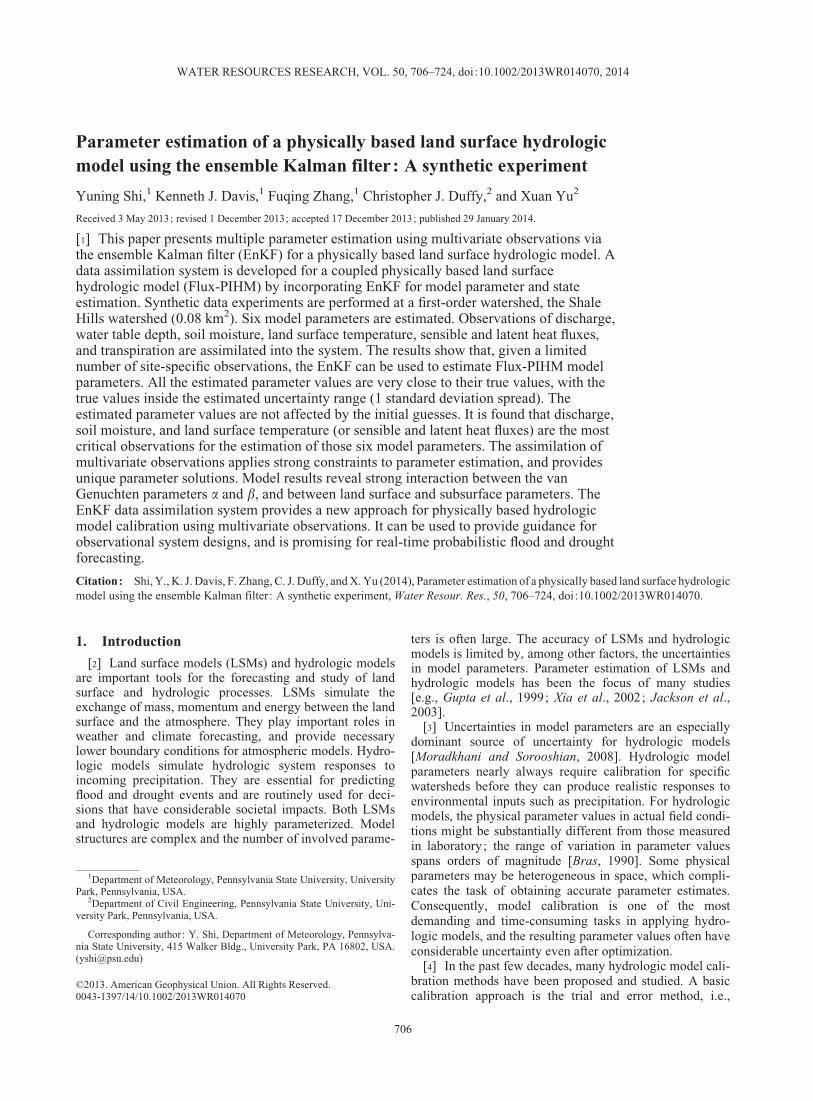
[19] The workflow of Flux-PIHM parameter estimationusing EnKF is presented in Figure 1:

[20] 1. At the beginning, initial conditions of state varia-bles (x), or model parameters (A), or both are perturbed togenerate initial conditions and model parameters for the ithensemble member, xi and /i.

[21] 2. In the forecast step, each ensemble member is putinto Flux-PIHM to perform hydrologic and land surfaceforecasting.

[22] 3. When observations are available, the forecastedvariables for each ensemble member xf

i and the parametersfor each ensemble member /f

i are updated using EnKF byassimilating the observations.

[23] 4. The covariance relaxation method (equation (3))is applied to both model variables and parameters whileconditional covariance inflation [Aksoy et al., 2006] isapplied to model parameters if needed.

[24] 5. The quality control process is applied to the anal-ysis of model variables xa

i and model parameters /ai to

ensure both model variables and model parameters are con-strained in their physically allowable or plausible ranges.

The obtained state variables xQCi and parameters /QC

i areused as initial conditions and parameters for the next fore-cast step.

[25] 6. Steps 2–5 are repeated until the end ofsimulation.

[26] In the current methodology, EnKF analysis does notconserve mass and energy. Mass and energy conservationcan be achieved by using constrained EnKF [Pan andWood, 2006], which adds another constraint filter for massand energy budgets after EnKF updates, or by simplyrescaling model variables using the ratio between the priortotal mass (energy) and the posterior total mass (energy).Those methods both depend on the linearization of massand energy budget equations. The rescaling method hasbeen tested with Flux-PIHM (results are not shown here),and the system needs a longer adjustment period whenmass and energy conservation is applied. Because theobjective of the current data assimilation system is to esti-mate the parameter values, mass and energy conservationdoes not need to be strictly satisfied at analysis steps.Therefore, mass and energy conservation is not applied tothe current data assimilation and parameter estimationexperiments, but the option is available if so desired.

3. Experimental Setup

[27] The Flux-PIHM EnKF data assimilation system isimplemented at the Shale Hills watershed in central Penn-sylvania (Figure 2). The Susquehanna Shale Hills CriticalZone Observatory (SSHCZO) now exists in this watershed.A real-time hydrologic monitoring network (RTHnet) isoperating in the SSHCZO. The Shale Hills watershed (0.08km2) is a small-scale, forested, V-shaped catchment, char-acterized by relatively steep slopes and narrow ridges. Thesurface elevation varies from 256 m above sea level at thewatershed outlet to 310 m above sea level at the ridge top.The Shale Hills watershed is in temperate continental cli-mate, with a mean annual temperature of 10�C and a meanannual precipitation of 107 cm. Precipitation is relativelywell-distributed year-round. A first-order headstream formswithin the watershed, which is mostly dry during summermonths. The small scale and the steep slopes make it chal-lenging to perform model calibration, because streamflowand groundwater have larger variability in low-order water-sheds than in larger basins [Reed et al., 2004]. Shi et al.[2013a] have manually calibrated and evaluated Flux-PIHM at the Shale Hills watershed. The same domain setupand meteorological forcing as in Shi et al. [2013a] areadopted in this study. For the synthetic experiment, a truthmodel run is performed using the manually calibratedparameter values from Shi et al. [2013a] starting from therelaxation mode. The truth run starts from 0000 UTC 1 Jan-uary 2009. The period from 0000 UTC 1 January to 1700UTC 1 March 2009 is the spin-up period. After the spin-up,predictions from the truth run are used to generate syntheticobservations from 1700 UTC 1 March to 0000 UTC 1August 2009. The outputs from 0000 UTC 1 August to0000 UTC 1 December 2009 are used to evaluate the esti-mated model parameters.

[28] The hourly predictions of the following observablevariables from the truth run are used:

[29] 1. Outlet discharge rate (Q) ;

Initialconditions

Ensemble members

Forecast Analysis

Constrainedanalysis

Perturbation

Flux-PIHM EnKF Quality control

Observations

Figure 1. Flowchart of Flux-PIHM data assimilationframework for parameter and state estimation.

SHI ET AL.: PARAMETER ESTIMATION USING ENKF

710

[30] 2. Water table depth at the model grid that repre-sents the RTHnet wells (WTD);

[31] 3. Integrated soil moisture content over the soil col-umn at the model grid that represents the RTHnet wells(SWC);

[32] 4. Land surface temperature averaged over themodel domain (Tsfc) ;

[33] 5. Sensible heat flux averaged over the modeldomain (H) ;

[34] 6. Latent heat flux averaged over the model domain(LE); and

[35] 7. Canopy transpiration rate averaged over themodel domain (Et).

[36] To account for the observation uncertainties, syntheticobservations are obtained by adding Gaussian white noise tothe true time series. The imposed observation errors for dif-ferent observation types are independent. The white noiseadded to the truth (Table 2) is designed to represent realisticerrors in observational precision. Note that these errors donot represent potential systematic biases in observations.WTD, for example, is a highly precise measurement, but canhave systematic offsets that are considerably larger than theprecision of the measurement. We do not attempt to simulatethe impact of systematic errors on the EnKF system in thismanuscript. We determine observational precisions with acombination of instrument specifications and prior literature.

[37] At the Shale Hills watershed, discharge is measuredwith a V-notch weir at the outlet of the catchment. ACampbell CS420-L (0–10 psi) pressure transducer meas-ures the water level, which is then converted to dischargerate using a rating curve developed by Nutter [1964] for theV-notch weir at the Shale Hills watershed. The calibratedrating curve is:

Q5

2446:5831025:561181:6722778:15x2

; 0 < x � 0:034 m;

3:083104x2:46; 0:034 m < x � 0:100 m;

3:123106x4:47; x > 0:100 m;

8>><>>:

(5)

where x is the measured water level (m), and Q is the dis-charge rate (m3 d21). The precision of Campbell CS420-Ltransducers is 60.1% full scale (0–10 psi), which is equiva-lent to about 7 mm of water level [Campbell Scientific Inc.,2007]. Figure 3a shows the rating curves with 7 mm errorsin measured water level (Q1 and Q2). Clark et al. [2008]found that converting discharge to log space improvesEnKF performance. Their strategy is adopted in this study.Prior to each analysis step, the discharge observation Qo isconverted to ln ðQo1�Þ, and for each ensemble member i,model discharge forecast Qf

i is converted to ln ðQfi 1�Þ,

where � is a very small discharge rate (set to 1024 m3 d21

in this study) used to avoid taking the logarithm of a zerodischarge rate. The precision of discharge measurement inlog space at the Shale Hills watershed is approximated by

rln Q50:5 ln Q12ln Q2ð Þ; (6)

as shown in Figure 3b. To simplify the calculation of rln Q,two linear segments are used to fit the rln Q curve:

Figure 2. Grid setting for the Shale Hills watershed model domain. The watershed boundary, streampath, surface elevation, and locations of RTHnet measurements used in this study are shown.

Table 2. Standard Deviation of Gaussian White Noise Added toEach Observation Data Set

Data SetStandard Deviation ofGaussian White Noise

Outlet discharge rate (m3 d21) Equation (7)a

Water table depth (m) 0.007 ma

Integrated soil moisture (m3 m23) 0.01 m3 m23b

Land surface temperature (�C) 1�Cc

Sensible heat flux (W m22) 10% of fluxd

Latent heat flux (W m22) 10% of fluxd

Transpiration rate (mm d21) 10% of fluxd

aPrecision of Campbell CS420-L pressure transducers.bPrecision of Decagon Echo2 EC-20 soil moisture sensors.cWan and Li [1997]; Yu et al. [2008]; Coll et al. [2009]; Wang and

Liang [2009].dLenschow and Stankov [1986]; Lenschow et al. [1994]; Baldocchi

et al. [1996]; Finkelstein and Sims [2001]; Baldocchi [2003]; Richardsonet al. [2006]; Salesky et al. [2012].

SHI ET AL.: PARAMETER ESTIMATION USING ENKF

711

rln Q520:509 ln Q1�ð Þ11:448; Q1� � 8:731m3d21;

20:0332 ln Q1�ð Þ10:417; Q1� > 8:731m3d21:

((7)

[38] Equation (7) is used in this study to estimate theobservation error of discharge in log space. The ground-water level at the RTHnet wells are also measured withCampbell CS420-L (0–10 psi) pressure transducers, with aprecision of 7 mm. The soil moisture contents are measuredusing Decagon Echo2 EC-20 soil moisture sensors. Czar-nomski et al. [2005] examined the precision of the EC-20sensors and found that the precision of which is about4.8%. Because the annual average soil moisture content atthe Shale Hills watershed is about 0.2 m3 m23, we thusassume that the precision of the soil moisture sensors is0.01 m3 m23. The observation error of land surface temper-ature is assumed to be 1.0�C, based on prior validations ofMODIS land surface temperature product [Wan and Li,1997; Yu et al., 2008; Coll et al., 2009; Wang and Liang,

2009]. The observation errors of sensible and latent heatfluxes (H and LE) are assumed to be 10% based on exten-sive prior study of the nature of random errors in eddycovariance flux measurements [Lenschow and Stankov,1986; Lenschow et al., 1994; Baldocchi et al., 1996; Fin-kelstein and Sims, 2001; Baldocchi, 2003; Richardsonet al., 2006; Salesky et al., 2012]. Careful assessment ofthe precision of watershed-scale transpiration measure-ments (Et) is lacking, so we have used the same precisionestimate as for eddy covariance flux measurements.

[39] The parameters to be estimated in this study andtheir a priori values are presented in Table 3: the effectiveporosity He, the van Genuchten [1980] soil parameter a,the van Genuchten soil parameter b, the Zilitinkevich[1995] parameter Czil, the minimum stomatal resistance Rc

min, and the reference canopy water capacity S. These sixparameters show high distinguishability, observability, andsimplicity [Zupanski and Zupanski, 2006; Nielsen-Gam-mon et al., 2010] in the parameter sensitivity analysis [Shiet al., 2013b]. High distinguishability, observability, andsimplicity have been proven critical for EnKF parameterestimation [Nielsen-Gammon et al., 2010; Hu et al., 2010;Aksoy et al., 2006]. Therefore these six parameters areselected for EnKF parameter estimation. The physicallyplausible ranges of those parameters are obtained from pre-vious studies [e.g., Beven and Binley, 1992; Chen et al.,1997; Gupta et al., 1999; Eckhardt and Arnold, 2001;Anderton et al., 2002; Tang et al., 2006] and experiencefrom manual calibration [Shi et al., 2013a], and are pre-sented in Table 3. Details about those parameters can befound in Shi et al. [2013a, 2013b]. The parameters that arenot estimated are set to their manually calibrated values asin Shi et al. [2013a]. The Flux-PIHM Shale Hills watershedmodel domain has 535 triangular grids and 20 river seg-ments. Including the variables in Table 1 and the sixparameters (global calibration coefficients) in Table 3, thetotal dimension of the joint state-parameter vector is 7002.

[40] Several test cases are used for the synthetic dataexperiments (Table 4). For each test case, a total of 30ensemble members are involved. Ensemble runs with 50ensemble members have been tested, but the increase inensemble members does not measurably improve theresults in terms of the mean squared errors of the estimatedparameters. Therefore, 30 ensemble members are used toreduce computational cost. To generate different ensemblemembers, calibration coefficients of those six parametersare randomly perturbed within their plausible ranges. For

Figure 3. (a) Rating curves for the Shale Hills watershedoutlet V-notch weir and (b) representative discharge mea-surement error. The dashed and dotted lines in Figure 3arepresent rating curves with 7 mm error in measured waterlevel. The dashed line in Figure 3b represents the manualfitting curve for the representative error.

Table 3. Flux-PIHM Model Parameters to be Estimated and the Plausible Ranges of Their Calibration Coefficients

A Priori Value

Soil Type Range of CalibrationParameter Description Weikert Berks Rushtown Blairton Ernest Coefficient

He Effective porosity (m3 m23) 0.48 0.32 0.33 0.29 0.34 0.3–1.2a Van Genuchten soil parameter (m21) 2.46 2.51 2.84 2.79 3.27 0–2.5b Van Genuchten soil parameter 1.20 1.21 1.33 1.33 1.32 0.95–2.5

Vegetation TypeDecidous Forest Evergreen Forest Mixed Forest

Rc min Minimum stomatal resistance (s m21) 100 150 125 0.3–1.2S Reference canopy water storage (mm) 0.20 0.20 0.20 0–5

OtherCzil Zilitinkevich parameter 0.10 0.1–10

SHI ET AL.: PARAMETER ESTIMATION USING ENKF

712

each parameter (calibration coefficient) /, the values arerandomly drawn from a Gaussian distribution, with an ini-tial standard deviation of r050:2 /max 2/minð Þ. The initialensemble means for different test cases are presented inTable 4. The parameter Czil is perturbed in log spacebecause the plausible range for Czil spans orders of magni-tude. The correlation coefficients between different param-eters among all ensemble members are examined toguarantee that the initial correlation coefficient (absolutevalue) between any two of those parameters is �0.25.Same as the truth run, all of the ensemble members startfrom 0000 UTC 1 January 2009, and the calibration periodis from 1700 UTC 1 March to 0000 UTC 1 August 2009.All model runs start from saturation in relaxation mode.Because accurate in situ meteorological observations (e.g.,precipitation and temperature) are collected at this small-scale watershed (0.08 km2), we assume that the uncertain-ties in meteorological forcing are negligible, comparedwith the uncertainties in model parameters. Therefore, themeteorological forcing used for each ensemble member isthe same as for the truth run. The first set of observations isassimilated at 1700 UTC 1 March 2009. We choose toassimilate observations at the midday time steps (1700UTC) because the land surface fluxes have the strongestcorrelation with model parameters at midday. Thus, assimi-lating observations at midday is the most effective in cor-recting the biases in model states and parameters. Differentassimilation intervals (24, 48, 72, and 96 h) and differentcombinations of observations are tested (Table 4).

[41] The assumption of homogeneous atmospheric forc-ing is well justified given the very small (microscale) gridsizes in our model [Mahrt, 2000]. We conducted a singletest of our assumption that meteorological forcing uncer-tainties are negligible and found no impact of 10% randomerrors in precipitation, the meteorological input variablemost likely to suffer from random observational errors.

[42] Each parameter is judged to have converged whenthe standard deviation of the parameter decreases to 0.25r0, where 0.25 r0 is also the threshold specified for the con-ditional covariance inflation method. The temporal averageof the ensemble mean after convergence is considered to bethe calibrated value of each parameter. If the parameterdoes not converge during the calibration period, i.e., thestandard deviation of parameter is always >0.25 r0, thetemporal average of the parameter values between 0000UTC 1 July and 0000 UTC 1 August 2009 is calculated asthe calibrated value for the parameter.

[43] Flux-PIHM runs using the calibrated parameter val-ues from different test cases are performed and comparedwith the truth run to evaluate the estimated parameter val-ues. Besides those test cases in Table 4, a NoPE (no param-eter estimation) run is also performed. In the NoPEevaluation run, the calibration coefficients for those sixparameters are set to 1.0, which means those parametersare uncalibrated and the a priori parameter values in Table 3are used. All of the evaluation runs start from 0000 UTC 1

January 2009 from the relaxation mode. Model forecastsfrom 0000 UTC 1 August to 0000 UTC 1 December 2009,which is the period right after the calibration period, areused to evaluate the model performance. The predictions ofall observable variables are compared with the truth run.For hydrologic variables (Q, WTD, and SWC), compari-sons are made at every hour. For land surface variables(Tsfc, H, LE, and Et), comparisons are made only at 1700UTC on every day to filter out the diurnal cycles of surfacefluxes.

4. Results

4.1. Accuracy of EnKF Parameter Estimation

[44] The control run is used to examine the accuracy ofEnKF parameter estimation. In the control run, the initialguess of parameter values is at the center of their uncer-tainty ranges (Table 4). Figure 4 presents the true valuesand the temporal evolutions of the parameters from thecontrol run. All of the six parameters approach their truevalues (Figure 4). After about 10 observation cycles (about1 month simulations after the first set of observations isassimilated), all parameters are very close to their true val-ues, with the true values inside or close to the 1 standarddeviation (1-r) spreads. The estimated parameter valuesoscillate around the true values after they approach them(Figure 4).

[45] The standard deviations of those parameters aredecreasing over time before convergence (Figure 4), whichindicates the decrease in parameter uncertainties. All of theparameters have converged (i.e., the standard deviations ofthe parameters have decreased to 0.25 r0). Among the sixparameters, the standard deviations of a, b, and Czil dropthe fastest because of their strong correlations with statevariables [Shi et al., 2013b]. The standard deviations of He

and S drop the slowest because the identifiability of He isonly high at discharge peaks, and S is only effective whenthe canopy is wet, as found in Shi et al. [2013b].

Table 4. Initial Ensemble Mean Of Parameters, Assimilation Intervals, and Assimilated Observations of Different Test Casesa

Case Initial Ensemble Mean Assimilation Interval Q WTD SWC Tsfc H LE Et

Control run (CR) 0:5 /min 1/maxð Þ 72 h X X X X X X XCase1 0:5 /min 1/maxð Þ2r0 72 h X X X X X X XCase2 0:5 /min 1/maxð Þ1r0 72 h X X X X X X X96 h Same as CR 96 h X X X X X X X48 h Same as CR 48 h X X X X X X X24 h Same as CR 24 h X X X X X X XQ Same as CR 72 h XSSHCZO Same as CR 72 h X X X X XNoSWC Same as CR 72 h X X X X X XNoWTD Same as CR 72 h X X X X X XQST Same as CR 72 h X X X

aX indicates the listed observation is assimilated, and blank indicates the observation is not assimilated.

SHI ET AL.: PARAMETER ESTIMATION USING ENKF

713

[46] Figure 5 demonstrates the capability of EnKF instate estimation, and two representative observable varia-bles Q and Tsfc are presented. Figure 5 shows that EnKF iseffective in optimizing model variables. It is especiallyapparent in the second assimilation cycle for Q (Figure5a): although the prior (ensemble prediction) of Q has arelatively large error, EnKF successfully corrects the error

in Q and significantly improves the estimate. Before thecalibration period, the model errors and uncertainties (espe-cially for Tsfc) are both relatively large. When more obser-vations are assimilated, the errors and uncertainties ofmodel parameters decrease (Figure 4), thus the modelerrors and uncertainties of variables decrease (Figure 5).Figure 5a shows some spin-up effects in Q. There is always

Figure 4. True values and temporal evolutions of parameters from the control run. The dashed linesrepresent the true parameter values, and the shaded areas represent the one standard deviation (1-r)spread.

Figure 5. Temporal evolution of the ensemble prediction of (a) discharge and (b) mid-day land surfacetemperature in the control run from 0000 UTC 1 February to 0000 UTC 1 May 2009. The shaded arearepresents the 1-r spread of the ensemble prediction.

SHI ET AL.: PARAMETER ESTIMATION USING ENKF

714

an increase in model error and uncertainty at the beginningof each forecast cycle, because the update of state variablesand parameters via EnKF disrupts the equilibrium in thesystem. This spin-up effect is more significant in hydro-logic variables (Q, WTD, and SWC) than in land surfacevariables (Tsfc, H, LE, and Et). Figure 5b shows an over-shooting effect. When the first set of observations is assimi-lated, the analysis (posterior) of Tsfc overshoots theobservation of Tsfc, due to the effects of other types ofobservations on Tsfc.

[47] The calibrated parameter values are listed inTable 5. Errors of calibrated parameter values in the controlrun are all <0.25 r0. Because 0.25 r0 is the threshold speci-fied for the conditional covariance inflation method, anerror< 0.25 r0 indicates that the true parameter value iswithin the 1-r spread of ensemble mean after convergence.The comparisons between the evaluation run using the cali-brated parameter set and the ‘‘truth’’ are presented in Fig-ure 6. Note that the evaluation run is the deterministicmodel run using the calibrated parameter set in Table 5, butnot the ensemble calibration run shown in Figure 5. Com-pared with the NoPE run, calibrated parameter values fromthe control run significantly improve the model predictions,especially for the hydrologic variables (Figure 6). Predic-tions of all observable variables from the evaluation runagree well with the truth (Figure 6). Both the correlationcoefficients and the normalized root-mean-square errors(RMSEs) of the predictions are very close to 1.0. The meanbiases in different predictions are negligible.

4.2. Optimal Assimilation Interval

[48] The control run (with a 72 h assimilation interval),96, 48, and 24 h cases (Table 4) are used to find the optimalassimilation interval for parameter estimation. The same 30ensemble members are used to start each test case. Figure 7presents the true values and the temporal evolutions of theparameters from those test cases. Generally, as shown inFigure 7, the performance of parameter estimation is theworst when the assimilation interval is 24 h. For the 24 hcase, EnKF keeps increasing a, and decreasing b and He tocompensate the spin-up effect. Differences among 48 h,control run (72 h), and 96 h are not significant in Figure 7.

[49] The RMSEs and absolute biases of the estimatedparameter values for those test cases after convergence arecalculated to quantify the effects of assimilation intervals.The results are presented in Figure 8. The RMSEs pre-sented here are normalized by the RMSEs in the control

run. For all the parameters except for Czil, RMSEs andabsolute biases decrease monotonically when the assimila-tion interval increases from 24 to 72 h (Figure 8). For theparameter Czil, there is no obvious tendency with respect tothe assimilation interval. This spin-up effect is the mostprominent in the parameter a. When the assimilation inter-val increases from 72 to 96 h, no significant improvementin parameter estimation (in terms of RMSEs and absolutebiases) is found (Figure 8). It suggests that the assimilationinterval of 72 h is long enough to eliminate the impacts ofspin-up effect in the synthetic experiments. Although lon-ger assimilation intervals would also be sufficient to avoidthe spin-up effect (e.g., the 96 h case), longer assimilationintervals mean that fewer observations would be assimi-lated into the system during the same simulation period.Therefore, 72 h is the optimal assimilation interval for thesynthetic experiments at the Shale Hills watershed.

4.3. Sensitivity to Initial Parameter Values

[50] The control run, Case1, and Case2 (Table 4) areused to demonstrate the sensitivity of EnKF parameter esti-mation to different initial parameter values. Figure 9presents the true values and the temporal evolutions of theestimated parameters from those three test cases. In all ofthe three test cases, all six parameters approach their truevalues (Figure 9). Starting from different initial guesses, theestimated parameter values from different test cases becomeclose after about 2 month simulation and data assimilation.The temporal fluctuations of parameter values from differenttest cases are similar. Those fluctuations are mostly causedby the observation errors in the synthetic observations.

[51] All of the parameters from those three test caseshave converged (i.e., the standard deviations of the parame-ters have decreased to 0.25r0). Errors of the calibratedparameter values from those three test cases are all <0.25r0 (Table 5), indicating that the true parameter values arewithin the 1-r spread of the ensemble prediction after con-vergence. The comparisons between the evaluation runsusing the calibrated parameter sets and the truth are pre-sented in Figure 6. The performances of the evaluation runsusing Case1 and Case2 parameters are very similar to thecontrol run, and show significant improvements in modelpredictions over the NoPE run.

4.4. Efficiency of Assimilating Different Observations

[52] The control run, Q, SSHCZO, NoSWC, NoWTD,and QST cases are compared to illustrate the efficiency of

Table 5. Calibrated Parameter Calibration Coefficients From Different Test Casesa

Case He a b Czil Rc min S

True value 0.52 1.50 1.30 0.70 0.50 2.00Control run 0.51 1.48 1.32 0.70 0.47 2.02Case1 0.52 1.59 1.30 0.71 0.48 1.87Case2 0.54 1.50 1.32 0.70 0.48 1.91Q (0.49) 0.81 (1.51) (0.46) (0.60) (1.93)SSHCZO 0.49 1.46 1.33 0.88 0.45 (2.40)NoSM 0.52 0.91 1.46 0.70 0.48 2.01NoWTD 0.48 1.46 1.33 0.70 0.47 1.89QST 0.48 1.38 1.36 0.66 0.52 (3.44)NoPE 1.00 1.00 1.00 1.00 1.00 1.00

aCalibrated values in bold font indicate that the estimated values have errors >0.25r0. Estimated values in parentheses indicate that the estimation ofthe parameter does not converge, i.e., the standard deviation of the parameter is always >0.25r0 during the calibration period.

SHI ET AL.: PARAMETER ESTIMATION USING ENKF

715

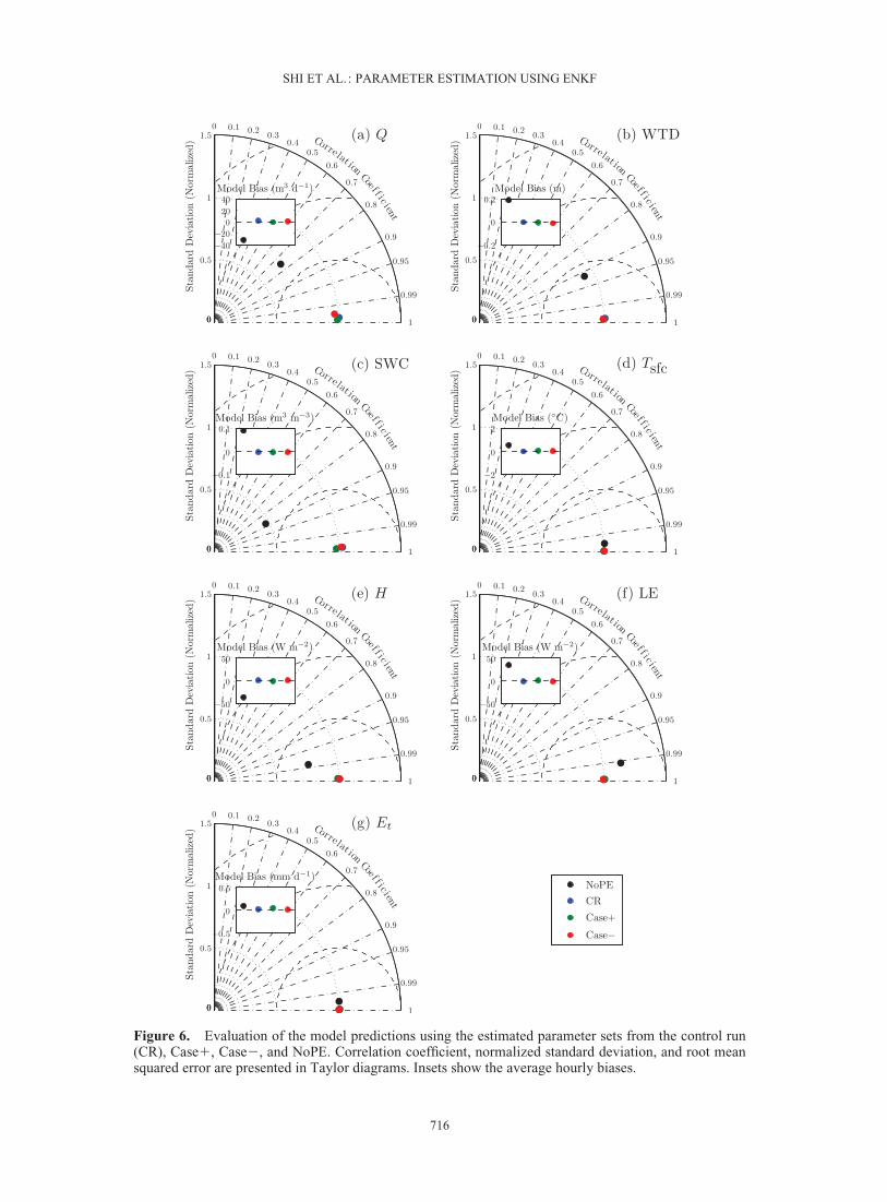
Figure 6. Evaluation of the model predictions using the estimated parameter sets from the control run(CR), Case1, Case2, and NoPE. Correlation coefficient, normalized standard deviation, and root meansquared error are presented in Taylor diagrams. Insets show the average hourly biases.

SHI ET AL.: PARAMETER ESTIMATION USING ENKF

716

assimilating different observations. Among them, the Qcase only assimilates the discharge observations as in mostprevious studies of hydrologic model calibrations. TheSSHCZO case uses those synthetic observations that repre-sent the observations available at the Shale Hills CriticalZone Observatory (SSHCZO) within the Shale Hills water-shed. The NoSWC and NoWTD test cases eliminate soilmoisture and water table depth observations, respectively.The QST case assimilates the discharge, soil moisture, andland surface temperature observations, which are assumedto be the essential observations for Flux-PIHM at the ShaleHills watershed. Figure 10 presents the true values and the

temporal evolutions of the parameters from those test cases.The same 30 ensemble members are used to start each testcase. The calibrated values for each parameter in differenttest cases are listed in Table 5. The comparisons of observ-able variables between evaluation runs using the calibratedparameter sets and the truth are presented in Figure 11.

[53] Figure 10 and Table 5 show that when discharge isthe only observation data set assimilated into the system,EnKF can only provide good estimates for model parame-ters He and S, the errors of which are <0.25r0. Except forthe parameter a, the other calibrated parameters do not con-verge in this test case (Table 5), and the calibrated parame-ter values still have relatively large uncertainty. Comparedwith the NoPE evaluation run, although this test case (Q)provides good estimates for only two of the six modelparameters, the calibrated parameters from this test casestrongly improve the prediction of discharge (Figure 11a).Comparison of the discharge prediction with the truthshows a high correlation coefficient (about 0.99) and a nor-malized standard deviation comparable with other testcases, although this test case underestimates the total dis-charge by 10.31 m3 d21 (10.59%; Figure 11a). The assimi-lation of discharge observations helps the system obtainmodel parameters that can produce reasonable dischargepredictions. For the other two hydrologic variables (WTDand SWC), the correlation coefficients are only better thanthe NoPE run, but lower than the other test cases, especiallyfor SWC. It indicates that parameters obtained in the Qcase have limited ability in resolving the temporal patternof wetting and drying in WTD and SWC. The SWC simula-tion also significantly overestimates the amplitude of tem-poral variation in SWC, and has a relatively large modelbias. Due to the lack of land surface variable observations,estimations of land surface parameters (Rc min and Czil) arepoor (Figure 10 and Table 5). The calibrated parameters in

Figure 7. True values and temporal evolutions of parameters from the control run (CR; 72 h), 96, 48,and 24 h. The dashed lines represent the true parameter values.

Figure 8. RMSEs and absolute biases of the estimatedparameter values after convergence. RMSEs from all testcases are normalized by the RMSEs in control run (CR).

SHI ET AL.: PARAMETER ESTIMATION USING ENKF

717

this test case (Q) cannot reproduce the temporal variationof land surface variables well (Figures 11d–11g).

[54] When SWC is not assimilated into the system (theNoSWC test case), EnKF cannot provide good estimates ofa and b, and the errors in a is much >0.25r0 (Figure 10and Table 5). The sensitivity analysis of Flux-PIHMshowed that the effect of a is the most significant in SWC[Shi et al., 2013b]. In this test case, EnKF underestimates

a, and thus produces a relatively large bias in SWC (Figure11c). Although the parameter values of a and b estimatedin this test case have relatively large errors, the dischargeand WTD predictions using these estimated parameter val-ues are comparable to the control run.

[55] The calibrated parameter values from the NoWTDcase are very close to the control run (Figure 10 andTable 5). The predictions using those calibrated parameter

Figure 9. True values and temporal evolutions of parameters from the control run (CR), Case1, andCase2. The dashed lines represent the true parameter values.

Figure 10. Same as Figure 9, but for the control run (CR), Q, SSHCZO, and NoSWC, NoWTD, andQST.

SHI ET AL.: PARAMETER ESTIMATION USING ENKF

718

Figure 11. Same as Figure 6, but for the control run (CR), Q, SSHCZO, NoSWC, NoWTD, QST, andNoPE.

SHI ET AL.: PARAMETER ESTIMATION USING ENKF

719

values are as good as the control run (Figure 11), whichsuggests that effect of assimilating WTD observations islimited.

[56] The QST case is used to test the most essentialobservations. Assimilating only three types of the sevenavailable observations, the estimated parameter valuesfrom the QST case are close to the control run, except forthe parameter S, which does not converge during the cali-bration period (Figure 10 and Table 5). The evaluation runpredictions of the QST test case are comparable to othertest cases (Figure 11), although the calibrated parameter setproduces relatively large biases in discharge and transpira-tion rate compared with other test cases. On average, thistest case overestimates the discharge by 8.11% (Figure11a), and underestimates the midday transpiration by6.26% (Figure 11g).

[57] The SSHCZO case does not assimilate Tsfc and Et.The calibrated values of parameters, except for Rc min and S,are very close to the true values (Figure 10 and Table 5).The predictions of the hydrologic variables are almost asgood as in the control run (Figures 11a–11c). For the landsurface variables, the prediction of the SSHCZO case over-estimates Tsfc by 1.10�C, because observations of Tsfc arenot assimilated, but the predictions of H, LE, and Et are onlyslightly worse than the control run (Figures 11d–11g). Inspite of the lack of Tsfc and Et observations, the assimilationof H and LE are sufficient to represent land surface states.

4.5. Parameter Interaction

[58] Because EnKF is based on ensemble generation, therelationship among different ensemble members reveals theinteractions between model parameters. Table 6 presentsthe temporal average of correlation coefficients betweenthe estimated parameter values from 0000 UTC 1 June to0000 UTC 1 August 2009 for three different test cases.This period is chosen because all parameters from thosethree test cases have converged during this period. Most ofthe parameter pairs have relatively low correlation

coefficients between 20.2 and 10.2 after convergence(Table 6). Although the initial ensemble is generated suchthat the initial correlation coefficient (absolute value)between any two of the parameters is �0.25, there are threepairs of parameters, a-b, a-Rc min, and Czil-Rc min that showcorrelations (absolute values) >0.25 after convergence(Table 6). Among them, a-b and a-Rc min show relativelyhigh correlations in all three test cases. Because a and b arehydrologic parameters, and Czil and Rc min are land surfaceparameters, those three pairs of parameters, respectively,represent the interaction between hydrologic parameters,the interaction between land surface and subsurface, andthe interaction between land surface parameters.

5. Discussion and Conclusions

[59] This paper presents the multiple parameter estima-tion of a coupled physically based land surface hydrologicmodel (Flux-PIHM) using multivariate observations viaEnKF. Results demonstrate that, given a limited number ofsite-specific observations, the EnKF can be used to providegood estimates of Flux-PIHM model parameters, with asso-ciated uncertainties. The EnKF data assimilation systemdesigned in this study provides a new approach for physi-cally based hydrologic model calibration using multivariateobservations. The sequential parameter estimation can saveconsiderable manual labor required for the implementationof hydrologic models, especially physically based models,at different watersheds.

[60] The test cases with different assimilation intervalsshow that the spin-up effect degrades the accuracy of theestimated hydrologic parameters. The spin-up effect ismore prominent for the hydrologic parameters than theland surface parameters. In this study at the Shale Hillswatershed, the assimilation interval of 72 h is found to beoptimal for the synthetic experiments.

[61] The performance of the test case Q indicates thatassimilating discharge alone can improve the prediction ofdischarge, however, the improvement is limited comparedwith other test cases. The predictions of subsurface varia-bles (especially SWC) and land surface variables in thistest case are poor compared with other test cases (Figure11). The prediction of discharge can be significantlyimproved when SWC observations are assimilated. Thosefindings agree with the findings of Camporese et al.[2009a, 2009b], Bailey and Ba�u [2010], and Lee et al.[2011]. This test case (Q) shows that assimilating dischargeobservation alone cannot provide reliable land surfaceparameter (Czil and Rc min) estimation.

[62] The effect of WTD observations is not strong whendischarge and SWC observations are assimilated. At theShale Hills watershed over 80% of annual discharge comesfrom subsurface runoff [Shi et al., 2013a], thus the tempo-ral variations of discharge and WTD are well correlated. Inaddition, WTD and SWC observations are also highly cor-related [Shi et al., 2013a]. Therefore, WTD is not an inde-pendent data set, and the effect of WTD observations isvery limited at this small watershed when discharge andSWC observations are both assimilated.

[63] The test cases QST and SSHCZO show that bothTsfc and surface heat fluxes are good indicators of land sur-face states. Assimilation of either Tsfc or surface heat fluxes

Table 6. Average Correlation Coefficients Between EstimatedParameter Values From 0000 UTC 1 June to 0000 UTC 1 August2009 in Three Different Test Casesa

He a b Czil Rc min S

He 1.00 20.04 20.06 20.02 0.07 20.061.00 0.10 20.11 0.02 0.03 0.001.00 20.03 20.03 0.01 0.02 20.02

a 1.00 20.47 0.08 20.29 0.061.00 20.36 0.00 20.26 20.061.00 20.31 0.02 20.45 20.02

b 1.00 20.09 20.05 0.001.00 20.06 20.05 0.051.00 20.07 0.11 0.04

Czil 1.00 20.26 0.001.00 20.20 0.031.00 20.25 20.02

Rc min 1.00 20.201.00 20.161.00 20.03

S 1.001.001.00

aThe correlation coefficients shown in each cell are in sequence for con-trol run, Case1, and Case2 (from top to bottom).

SHI ET AL.: PARAMETER ESTIMATION USING ENKF

720

is sufficient for land surface parameter estimation. The testcase QST also demonstrates that Q, SWC, and Tsfc are theessential observations for the estimation of those six modelparameters at the Shale Hills watershed. The SSHCZO testcase assimilates observations which are currently availableat the Shale Hills watershed. The results are very encourag-ing. It indicates that using the currently available observa-tion data sets for real data EnKF parameter estimation ispromising.

[64] There are several test cases that do not assimilate Et

observations: the test cases Q, SSHCZO, and QST. Resultsfrom those test cases show that as long as Tsfc or surfaceheat fluxes are assimilated into the system, the system isable to obtain model parameters that could provide reason-ably good Et prediction (Figure 11g). Therefore, the mea-surement of Et is not critical for model calibration purpose.

[65] Results from different test cases imply that theassimilation of multivariate observations improves theaccuracy of parameter estimation, and provides uniqueparameter solutions. For example, when SWC observationsare not assimilated into the system (NoSWC and Q testcases), EnKF cannot provide accurate estimates of the vanGenuchten parameters (Table 5), although both test casesprovide good discharge predictions (Figure 11a). Moreinterestingly, the a and b values estimated for those twotest cases (NoSWC and Q test cases) are very close (Table5). From the equifinality [Beven, 1993] perspective, whenSWC is not assimilated, EnKF finds another point in the a-b space, which produces almost equally good dischargepredictions as the true parameter values. Only when SWCobservations are assimilated, can EnKF find the unique andaccurate solutions of a and b. The assimilation of multivar-iate observations can apply more constraints to modelparameters, avoid the difficulty brought by model equifinal-ity, and provide unique parameter solutions. By testing theinfluences of assimilated observations in synthetic experi-ments, the required observations to identify the uniqueparameter set can be found. The data assimilation systemdeveloped in this paper can thus be used to provide guid-ance of observational system designs.

[66] The EnKF provides the estimates of not only param-eter values and model states, but also their uncertainties.When more types of observations are assimilated into thesystem (e.g., the control run), the uncertainties estimatedby EnKF decrease faster. When only limited types of obser-vations are assimilated into the system (e.g., the Q,SSHCZO, and QST test cases), the uncertainties estimatedby EnKF decrease slowly, and some of the parameters donot even converge (Table 5). The uncertainties by EnKFresult from various sources, e.g., the uncertainties of obser-vations and model parameters. The quantification of uncer-tainties is very useful for practical application, because theaccurate estimates of uncertainty is required in the opera-tional flood and drought forecasting. This EnKF dataassimilation system provides the possibility to performreal-time online probabilistic forecasting using a determin-istic model, which explicitly accounts for uncertaintiesfrom different sources (e.g., parameter, model structure,meteorological forcing, and assimilated observations).

[67] It needs to be pointed out that those results are basedon a perfect model, perfect forcing data, and a perfectmodel domain configuration. Model structural errors,

forcing data errors, observation errors, and domain configu-ration errors (e.g., errors in input topography, soil map, andland cover map) would pose extra difficulties for parameterestimation using real data. The synthetic observations usedin this study have Gaussian errors with no biases, and thesynthetic errors only include the random instrumentalerrors. In reality, some observations (e.g., discharge andsurface heat fluxes) may have non-Gaussian errors, theMODIS land surface temperature observations may havesystematic biases [Wan et al., 2002; Wang et al., 2008],and the eddy covariance measurements fail to close theenergy budget [McNeil and Shuttleworth, 1975; Fritschenet al., 1992; Twine et al., 2000]. Moreover, the soil mois-ture and water table depth observations may have represen-tativity errors in addition to the instrumental errors. Thoseerrors are not accounted for in this study, and need to betaken into account for real data applications. Differentapproaches have been used to assimilate observationswhich have consistent biases, e.g., rescaling the observa-tions, subtracting the long-term means from observationsand predictions, or assimilating the tendencies of observa-tions instead of their absolute values [Hain et al., 2012;Mackaro et al., 2012]. The impact of non-Gaussian, non-zero-bias observations on Flux-PIHM parameter estima-tion, however, still needs to be tested.

[68] Although the initial parameters are perturbed inde-pendently, EnKF is able to identify the interacting parameters(Table 6). Results from the control run, Case1 and Case2reveal strong correlation between the van Genuchten parame-ters a and b (Table 6). The negative correlation foundbetween a and b in these three test cases agree with the resultsin other test cases. As shown in Table 6, whenever a is under-estimated, b is always overestimated, and vice versa. Thestrong correlation found between the van Genuchten parame-ters suggests strong interactions between those parameters.The interaction leads to model equifinality [Beven, 1993], andexplains why the test cases Q and NoSWC provide poor esti-mates of a and b but acceptable discharge predictions. Bald-win [2011] derived the van Genuchten parameters at 61 sitesin the Shale Hills watershed based on soil moisture observa-tions at different depths, and analyzed the spatial relationshipbetween the van Genuchten parameters. The results showedthat the correlation coefficient between the van Genuchtenparameters from all depths and locations is 20.28. The corre-lation coefficients between van Genuchten parameters at 10cm and 20 cm below ground reach 20.44 and 20.48, respec-tively. The correlation between the van Genuchten parametersestimated by EnKF agrees well with Baldwin [2011] observa-tional results.

[69] The relatively high correlation between the vanGenuchten parameter a and the minimum stomatal resist-ance Rc min (Table 6) suggests interaction between land sur-face and subsurface. The model sensitivity analysis showsthat the model soil moisture prediction is very sensitive tothe change in the parameter a [Shi et al., 2013b], and soilmoisture affects transpiration, which is also influenced byRc min. The parameters a and Rc min are therefore connectedthrough the effect of soil moisture on transpiration. Thecorrelations between the hydrologic and land surfaceparameters represent the interaction between the subsurfaceand land surface, which suggests that subsurface and landsurface systems are closely coupled.

SHI ET AL.: PARAMETER ESTIMATION USING ENKF

721

[70] The correlations between different parametersrevealed by the EnKF system are useful for the study of theinteraction between dynamic systems, and are useful forthe simplification of model parameterization schemes. Theability of EnKF to identify the interacting parameters andquantify the correlations between parameters suggests thatit may not be necessary to take into account the correlationbetween parameters when generating the initial ensemble.This is valuable because prior information describingparameter correlation is frequently not available.

[71] Acknowledgments. This research was supported by the NationalOceanic and Atmospheric Administration through grant NA10OAR4310166, and the National Science Foundation Shale Hills-Susquehanna Criti-cal Zone Observatory project through grant EAR 0725019. Logistical sup-port and/or data were provided by the NSF-supported Shale HillsSusquehanna Critical Zone Observatory.

ReferencesAksoy, A., F. Zhang, and J. W. Nielsen-Gammon (2006), Ensemble-based

simultaneous state and parameter estimation in a two-dimensional sea-breeze model, Mon. Weather Rev., 134(10), 2951–2970, doi:10.1175/MWR3224.1.

Anderson, J. L., and S. L. Anderson (1999), A Monte Carlo implementationof the nonlinear filtering problem to produce ensemble assimilations andforecasts, Mon. Weather Rev., 127(12), 2741–2758, doi:10.1175/1520-0493(1999)127¡2741:AMCIOT>2.0.CO;2.

Anderton, S., J. Latron, and F. Gallart (2002), Sensitivity analysis andmulti-response, multi-criteria evaluation of a physically based distributedmodel, Hydrol. Processes, 16(2), 333–353, doi:10.1002/hyp.336.

Annan, J. D. (2005), Parameter estimation using chaotic time series, Tellus,Ser. A, 57(5), 709–714, doi:10.1111/j.1600-0870.2005.00143.x.

Arulampalam, M. S., S. Maskell, N. Gordon, and T. Clapp (2002), A tuto-rial on particle filters for online nonlinear/non-Gaussian Bayesian track-ing, IEEE Trans. Signal Process., 50(2), 174–188, doi:10.1109/78.978374.

Aubert, D., C. Loumagne, and L. Oudin (2003), Sequential assimilation ofsoil moisture and streamflow data in a conceptual rainfall-runoff model,J. Hydrol., 280(1), 145–161, doi:10.1016/S0022-1694(03)00229-4.

Bailey, R., and D. Ba�u (2010), Ensemble smoother assimilation of hydrau-lic head and return flow data to estimate hydraulic conductivity distribu-tion, Water Resour. Res., 46, W12543, doi:10.1029/2010WR009147.

Baldocchi, D., R. Valentini, S. Running, W. Oechel, and R. Dahlman(1996), Strategies for measuring and modelling carbon dioxide and watervapour fluxes over terrestrial ecosystems, Global Change Biol., 2(3),159–168, doi:10.1111/j.1365-2486.1996.tb00069.x.

Baldocchi, D. D. (2003), Assessing the eddy covariance technique for eval-uating carbon dioxide exchange rates of ecosystems: Past, present andfuture, Global Change Biol., 9(4), 479–492, doi:10.1046/j.1365-2486.2003.00629.x.

Baldwin, D. (2011), Catchment-scale soil water retention characteristicsand delineation of hydropedological functional units in the Shale HillsCatchment, MS thesis, Pa. State Univ., University Park.

Beven, K. (1993), Prophecy, reality and uncertainty in distributed hydrolog-ical modelling, Adv. Water Resour., 16(1), 41–51, doi:10.1016/0309-1708(93)90028-E.

Beven, K., and A. Binley (1992), The future of distributed models: Modelcalibration and uncertainty prediction, Hydrol. Processes, 6(3), 279–298,doi:10.1002/hyp.3360060305.

Boyle, D. P., H. V. Gupta, and S. Sorooshian (2000), Toward improved cal-ibration of hydrologic models: Combining the strengths of manual andautomatic methods, Water Resour. Res., 36(12), 3663–3674, doi:10.1029/2000WR900207.

Bras, R. L. (1990), Hydrology: An Introduction to Hydrologic Science, 643pp., Addison-Wesley, Reading, Mass.

Cammalleri, C., and G. Ciraolo (2012), State and parameters update in acoupled energy/hydrologic balance model using ensemble Kalman filter-ing, J. Hydrol., 416–417, 171–181, doi:10.1016/j.jhydrol.2011.11.049.

Campbell Scientific Inc. (2007), CS420-L and CS425-L Druck’s ModelsPDCR 1830 and 1230 pressure transducers, Instr. Manual 12/07, PaloAlto, Calif.

Camporese, M., C. Paniconi, M. Putti, and P. Salandin (2009a), EnsembleKalman filter data assimilation for a process-based catchment scalemodel of surface and subsurface flow, Water Resour. Res., 45, W10421,doi:10.1029/2008WR007031.

Camporese, M., C. Paniconi, M. Putti, and P. Salandin (2009b), Compari-son of data assimilation techniques for a coupled model of surface andsubsurface flow, Vadose Zone J., 8(4), 837–845, doi:10.2136/vzj2009.0018.

Chen, F., and J. Dudhia (2001), Coupling an advanced land surface-hydrology model with the Penn State-NCAR MM5 modeling system.Part I : Model implementation and sensitivity, Mon. Weather Rev.,129(4), 569–585, doi:10.1175/1520-0493(2001)129¡0569:CAALSH>2.0.CO;2.

Chen, F., Z. Janjic, and K. Mitchell (1997), Impact of atmospheric-surfacelayer parameterizations in the new land-surface scheme of the NCEPmesoscale Eta numerical model, Boundary Layer Meteorol., 85(3), 391–421, doi:10.1023/A:1000531001463.

Chen, Y., and D. Zhang (2006), Data assimilation for transient flow in geo-logic formations via ensemble Kalman filter, Adv. Water Resour., 29(8),1107–1122, doi:10.1016/j.advwatres.2005.09.007.

Clark, M. P., D. E. Rupp, R. A. Woods, X. Zheng, R. P. Ibbitt, A. G. Slater,J. Schmidt, and M. J. Uddstrom (2008), Hydrological data assimilationwith the ensemble Kalman filter: Use of streamflow observations toupdate states in a distributed hydrological model, Adv. Water Resour.,31(10), 1309–1324, doi:10.1016/j.advwatres.2008.06.005.

Coll, C., Z. Wan, and J. M. Galve (2009), Temperature-based and radiance-based validations of the V5 MODIS land surface temperature product, J.Geophys. Res., 114, D20102, doi:10.1029/2009JD012038.

Crow, W. T., and E. F. Wood (2003), The assimilation of remotely sensedsoil brightness temperature imagery into a land surface model usingensemble Kalman filtering: A case study based on ESTAR measure-ments during SGP97, Adv. Water Resour., 26(2), 137–149, doi:10.1016/S0309-1708(02)00088-X.

Czarnomski, N. M., G. W. Moore, T. G. Pypker, J. Licata, and B. J. Bond(2005), Precision and accuracy of three alternative instruments for meas-uring soil water content in two forest soils of the Pacific Northwest, Can.J. For. Res., 35(8), 1867–1876, doi:10.1139/X05-121.

Dechmi, F., J. Burguete, and A. Skhiri (2012), SWAT application in inten-sive irrigation systems: Model modification, calibration and validation,J. Hydrol., 470–471, 227–238, doi:10.1016/j.jhydrol.2012.08.055.

Duan, Q., S. Sorooshian, and V. K. Gupta (1992), Effective and efficientglobal optimization for conceptual rainfall-runoff models, Water Resour.Res., 28(4), 1015–1031, doi:10.1029/91WR02985.

Eckhardt, K., and J. G. Arnold (2001), Automatic calibration of a distrib-uted catchment model, J. Hydrol., 251(1), 103–109, doi:10.1016/S0022-1694(01)00429-2.

Ek, M. B., K. Mitchell, Y. Lin, E. Rogers, P. Grummann, V. Koren, G.Gayno, and J. Tarpley (2003), Implementation of Noah land surfacemodel advances in the National Centers for Environmental Predictionoperational Mesoscale Eta Model, J. Geophys. Res., 108(D22), 8851,doi:10.1029/2002JD003296.

Evensen, G. (1994), Sequential data assimilation with a nonlinear quasi-geostrophic model using Monte Carlo methods to forecast error statistics,J. Geophys. Res., 99(C5), 10,143–10,162, doi:10.1029/94JC00572.

Evensen, G. (2003), The ensemble Kalman filter: Theoretical formulationand practical implementation, Ocean Dyn., 53(4), 343–367, doi:10.1007/s10236-003-0036-9.

Finkelstein, P. L., and P. F. Sims (2001), Sampling error in eddy correlationflux measurements, J. Geophys. Res., 106(D4), 3503–3509, doi:10.1029/2000JD900731.

Flores, A. N., R. L. Bras, and D. Entekhabi (2012), Hydrologic data assimi-lation with a hillslope-scale-resolving model and L band radar observa-tions: Synthetic experiments with the ensemble Kalman filter, WaterResour. Res., 48, W08509, doi:10.1029/2011WR011500.

Franchini, M. (1996), Use of a genetic algorithm combined with a localsearch method for the automatic calibration of conceptual rainfall-runoffmodels, Hydrol. Sci. J., 41(1), 21–39, doi:10.1080/02626669609491476.

Francois, C., A. Quesney, and C. Ottl�e (2003), Sequential assimilation ofERS-1 SAR data into a coupled land surface-hydrological model usingan extended Kalman filter, J. Hydrometeorol., 4(2), 473–487, doi:10.1175/1525–7541(2003)4¡473:SAOESD>2.0.CO;2.

Fritschen, L. J., P. Qian, E. T. Kanemasu, D. Nie, E. A. Smith, J. B.Stewart, S. B. Verma, and M. L. Wesely (1992), Comparisons of surfaceflux measurement systems used in FIFE 1989, J. Geophys. Res.,97(D17), 18,697–18,713, doi:10.1029/91JD03042.

SHI ET AL.: PARAMETER ESTIMATION USING ENKF

722

Gupta, H. V., L. A. Bastidas, S. Sorooshian, W. J. Shuttleworth, and Z.-L.Yang (1999), Parameter estimation of a land surface scheme using multi-criteria methods, J. Geophys. Res., 104(D16), 19,491–19,503, doi:10.1029/1999JD900154.

Gupta, V. K., and S. Sorooshian (1985), The relationship between data andthe precision of parameter estimates of hydrologic models, J. Hydrol.,81, 57–77, doi:10.1016/0022-1694(85)90167-2.

Hain, C. R., W. T. Crow, M. C. Anderson, and J. R. Mecikalski (2012), Anensemble Kalman filter dual assimilation of thermal infrared and micro-wave satellite observations of soil moisture into the Noah land surfacemodel, Water Resour. Res., 48, W11517, doi:10.1029/2011WR011268.

Han, E., V. Merwade, and G. C. Heathman (2012), Implementation of sur-face soil moisture data assimilation with watershed scale distributedhydrological model, J. Hydrol., 416, 98–117, doi:10.1016/j.jhydrol.2011.11.039.

Hendricks Franssen, H. J., H. P. Kaiser, U. Kuhlmann, G. Bauser, F.Stauffer, R. M€uller, and W. Kinzelbach (2011), Operational real-timemodeling with ensemble Kalman filter of variably saturated subsurfaceflow including stream-aquifer interaction and parameter updating, WaterResour. Res., 47, W02532, doi:10.1029/2010WR009480.

Houser, P. R., W. J. Shuttleworth, J. S. Famiglietti, H. V. Gupta, K. H.Syed, and D. C. Goodrich (1998), Integration of soil moisture remotesensing and hydrologic modeling using data assimilation, Water Resour.Res., 34(12), 3405–3420, doi:10.1029/1998WR900001.

Hu, X.-M., F. Zhang, and J. W. Nielsen-Gammon (2010), Ensemble-basedsimultaneous state and parameter estimation for treatment of mesoscalemodel error: A real-data study, Geophys. Res. Lett., 37, L08802, doi:10.1029/2010GL043017.

Ibbitt, R. P. (1970), Systematic parameter fitting for conceptual models ofcatchment hydrology, Ph.D. thesis, Univ. of London, London.

Jackson, C., Y. Xia, M. K. Sen, and P. L. Stoffa (2003), Optimal parameterand uncertainty estimation of a land surface model: A case study usingdata from Cabauw, Netherlands, J. Geophys. Res., 108(D18), 4583, doi:10.1029/2002JD002991.

Johnston, P. R., and D. H. Pilgrim (1976), Parameter optimization forwatershed models, Water Resour. Res., 12(3), 477–486, doi:10.1029/WR012i003p00477.

Kollat, J. B., and P. M. Reed (2006), Comparing state-of-the-art evolution-ary multi-objective algorithms for long-term groundwater monitoringdesign, Adv. Water Resour., 29(6), 792–807, doi:10.1016/j.advwatres.2005.07.010.

Kumar, M. (2009), Toward a hydrologic modeling system, PhD thesis, Pa.State Univ., University Park.

Kumar, S. V., R. H. Reichle, C. D. Peters-Lidard, R. D. Koster, X. Zhan,W. T. Crow, J. B. Eylander, and P. R. Houser (2008), A land surface dataassimilation framework using the land information system: Descriptionand applications, Adv. Water Resour., 31(11), 1419–1432, doi:10.1016/j.advwatres.2008.01.013.

Kurtz, W., H.-J. Hendricks Franssen, and H. Vereecken (2012), Identifica-tion of time-variant river bed properties with the ensemble Kalman filter,Water Resour. Res., 48, W10534, doi:10.1029/2011WR011743.

Lee, H., D. J. Seo, and V. Koren (2011), Assimilation of streamflow and in-situ soil moisture data into operational distributed hydrologic models:Effects of uncertainties in the data and initial model soil moisture states,Adv. Water Resour., 34(12), 1597–1615, doi:10.1016/j.advwatres.2011.08.012.

Leimer, S., T. Pohlert, S. Pfahl, and W. Wilcke (2011), Towards a new gen-eration of high-resolution meteorological input data for small-scalehydrologic modeling, J. Hydrol., 402(3), 317–332, doi:10.1016/j.jhydrol.2011.03.026.

Lenschow, D. H., and B. B. Stankov (1986), Length scales in the convectiveboundary layer, J. Atmos. Sci., 43(12), 1198–1209, doi:10.1175/1520-0469(1986)043¡1198:LSITCB>2.0.CO;2.

Lenschow, D. H., J. Mann, and L. Kristensen (1994), How long is longenough when measuring fluxes and other turbulence statistics?, J. Atmos.Oceanic Technol., 11(3), 661–673, doi:10.1175/1520-0426(1994)011¡0661:HLILEW>2.0.CO;2.

Liu, G., Y. Chen, and D. Zhang (2008), Investigation of flow and transportprocesses at the MADE site using ensemble Kalman filter, Adv. WaterResour., 31(7), 975–986, doi:10.1016/j.advwatres.2008.03.006.

L€u, H., T. Hou, R. Horton, Y. Zhu, X. Chen, Y. Jia, W. Wang, and X. Fu(2013), The streamflow estimation using the Xinanjiang rainfall runoffmodel and dual state-parameter estimation method, J. Hydrol., 480, 102–114, doi:10.1016/j.jhydrol.2012.12.011.

Mackaro, S. M., R. T. McNider, and A. P. Biazar (2012), Some physicaland computational issues in land surface data assimilation of satelliteskin temperatures, Pure Appl. Geophys., 169, 401–414, doi:10.1007/s00024-011-0377-0.

Mahrt, L. (2000), Surface heterogeneity and vertical structure of the bound-ary layer, Boundary Layer Meteorol., 96(1–2), 33–62, doi:10.1023/A:1002482332477.

McNeil, D. D., and W. J. Shuttleworth (1975), Comparative measurementsof the energy fluxes over a pine forest, Boundary Layer Meteorol., 9(3),297–313, doi:10.1007/BF00230772.

Montzka, C., V. R. N. Pauwels, H.-J. Hendricks Franssen, X. Han, and H.Vereecken (2012), Multivariate and multiscale data assimilation in ter-restrial systems: A review, Sensors, 12(12), 16,291–16,333, doi:10.3390/s121216291.

Moradkhani, H., and S. Sorooshian (2008), General review of rainfall-runoff modeling: Model calibration, data assimilation, and uncertaintyanalysis, in Hydrological Modelling and the Water Cycle, edited by S.Sorooshian et al., pp. 1–24, Springer, Heidelberg.

Moradkhani, H., S. Sorooshian, H. V. Gupta, and P. R. Houser (2005a),Dual state-parameter estimation of hydrological models using ensembleKalman filter, Adv. Water Resour., 28(2), 135–147, doi:10.1016/j.advwatres.2004.09.002.

Moradkhani, H., K.-L. Hsu, H. Gupta, and S. Sorooshian (2005b), Uncer-tainty assessment of hydrologic model states and parameters: Sequentialdata assimilation using the particle filter, Water Resour. Res., 41,W05012, doi:10.1029/2004WR003604.

Moran, M. S., C. D. Peters-Lidard, J. M. Watts, and S. McElroy (2004),Estimating soil moisture at the watershed scale with satellite-based radarand land surface models, Can. J. Remote Sens., 30(5), 805–826, doi:10.5589/m04-043.

Nielsen-Gammon, J. W., X. M. Hu, F. Zhang, and J. E. Pleim (2010), Eval-uation of planetary boundary layer scheme sensitivities for the purposeof parameter estimation, Mon. Weather Rev., 138(9), 3400–3417, doi:10.1175/2010MWR3292.1.

Nutter, W. L. (1964), Determination of the head-discharge relationship fora sharp-crested compound weir and a sharp-crested parabolic weir, MSthesis, Pa. State Univ., University Park.

Oudin, L., A. Weisse, C. Loumagne, and S. Le H�egarat-Mascle (2003),Assimilation of soil moisture into hydrological models for flood forecast-ing: A variational approach, Can. J. Remote Sens., 29(6), 679–686, doi:10.5589/m03-038.

Pan, M., and E. F. Wood (2006), Data assimilation for estimating the terres-trial water budget using a constrained ensemble Kalman filter, J. Hydro-meteorol., 7(3), 534–547, doi:10.1175/JHM495.1.

Pauwels, V. R. N., and G. J. M. De Lannoy (2006), Improvement of mod-eled soil wetness conditions and turbulent fluxes through the assimilationof observed discharge, J. Hydrometeorol., 7(3), 458–477, doi:10.1175/JHM490.1.

Pickup, G. (1977), Testing the efficiency of algorithms and strategies forautomatic calibration of rainfall-runoff models, Hydrol. Sci. Bull., 22(2),257–274, doi:10.1080/02626667709491716.

Pisinaras, V., C. Petalas, G. D. Gikas, A. Gemitzi, and V. A. Tsihrintzis(2010), Hydrological and water quality modeling in a medium-sizedbasin using the Soil and Water Assessment Tool (SWAT), Desalination,250(1), 274–286, doi:10.1016/j.desal.2009.09.044.

Pokhrel, P., and H. V. Gupta (2010), On the use of spatial regularizationstrategies to improve calibration of distributed watershed models, WaterResour. Res., 46, W01505, doi:10.1029/2009WR008066.

Qu, Y. (2004), An integrated hydrologic model for multi-process simula-tion using semi-discrete finite volume approach, PhD thesis, Pa. StateUniv., University Park.

Qu, Y., and C. J. Duffy (2007), A semidiscrete finite volume formulationfor multiprocess watershed simulation, Water Resour. Res., 43, W08419,doi:10.1029/2006WR005752.

Reed, S., V. Koren, M. Smith, Z. Zhang, F. Moreda, D.-J. Seo, and DMIPParticipants (2004), Overall distributed model intercomparison projectresults, J. Hydrol., 298(1), 27–60, doi:10.1016/j.jhydrol.2004.03.031.

Reichle, R. H., D. B. McLaughlin, and D. Entekhabi (2002a), Hydrologicdata assimilation with the ensemble Kalman filter, Mon. Weather Rev.,130(1), 103–114, doi:10.1175/1520-0493(2002)130¡0103:HDAW-TE>2.0.CO;2.

Reichle, R. H., J. P. Walker, R. D. Koster, and P. R. Houser (2002b),Extended versus ensemble Kalman filtering for land data assimilation, J.Hydrometeorol., 3(6), 728–740, doi:10.1175/1525–7541(2002)003¡0728:EVEKFF>2.0.CO;2.

SHI ET AL.: PARAMETER ESTIMATION USING ENKF

723

Richardson, A. D., et al. (2006), A multi-site analysis of random error intower-based measurements of carbon and energy fluxes, Agric. For.Meteorol., 136(1), 1–18, doi:10.1016/j.agrformet.2006.01.007.

Salamon, P., and L. Feyen (2009), Assessing parameter, precipitation, andpredictive uncertainty in a distributed hydrological model using sequen-tial data assimilation with the particle filter, J. Hydrol., 376(3), 428–442,doi:10.1016/j.jhydrol.2009.07.051.

Salesky, S. T., M. Chamecki, and N. L. Dias (2012), Estimating the randomerror in eddy-covariance based fluxes and other turbulence statistics:The filtering method, Boundary Layer Meteorol., 144(1), 113–135, doi:10.1007/s10546-012-9710-0.

Shi, P., C. Chen, R. Srinivasan, X. Zhang, T. Cai, X. Fang, S. Qu, X. Chen,and Q. Li (2011), Evaluating the SWAT model for hydrological model-ing in the Xixian watershed and a comparison with the XAJ model,Water Resour. Manage., 25(10), 2595–2612, doi:10.1007/s11269-011-9828-8.

Shi, Y., K. J. Davis, C. J. Duffy, and X. Yu (2013a), Development of acoupled land surface hydrologic model and evaluation at a critical zoneobservatory, J. Hydrometeorol., 14(5), 1401–1420, doi:10.1175/JHM-D-12-0145.1.

Shi, Y., K. J. Davis, F. Zhang, and C. J. Duffy (2013b), Evaluation of theparameter sensitivity of a coupled land surface hydrologic model at acritical zone observatory, J. Hydrometeorol., doi:10.1175/JHM-D-12-0177.1, in press.

Shih, D.-S., and G.-T. Yeh (2011), Identified model parameterization, cali-bration, and validation of the physically distributed hydrological modelWASH123D in Taiwan, J. Hydrol. Eng., 16(2), 126–136, doi:10.1061/(ASCE)HE.1943-5584.0000293.

Snyder, C., and F. Zhang (2003), Assimilation of simulated Doppler radarobservations with an ensemble Kalman filter, Mon. Weather Rev.,131(8), 1663–1677, doi:10.1175//2555.1.

Sorooshian, S., Q. Duan, and V. K. Gupta (1993), Calibration of rainfall-runoff models: Application of global optimization to the SacramentoSoil Moisture Accounting Model, Water Resour. Res., 29(4), 1185–1194,doi:10.1029/92WR02617.

Tang, Y., P. Reed, and T. Wagener (2006), How effective and efficient aremultiobjective evolutionary algorithms at hydrologic model calibration?,Hydrol. Earth Syst. Sci., 10, 289–307.

Twine, T. E., W. P. Kustas, J. M. Norman, D. R. Cook, P. R. Houser, T. P.Meyers, J. H. Prueger, P. J. Starks, and M. L. Wesely (2000), Correctingeddy-covariance flux underestimates over a grassland, Agric. For. Mete-orol., 103(3), 279–300, doi:10.1016/S0168-1923(00)00123-4.

van Genuchten, M. T. (1980), A closed-form equation for predicting thehydraulic conductivity of unsaturated soils, Soil Sci. Soc. Am. J., 44(5),892–898.

Vrugt, J., H. V. Gupta, B. �O. Nuall�ain, and W. Bouten (2006), Real-timedata assimilation for operational ensemble streamflow forecasting, J.Hydrometeorol., 7(3), 548–565, doi:10.1175/JHM504.1.

Wagener, T., N. McIntyre, M. J. Lees, H. S. Wheater, and H. V. Gupta(2003), Towards reduced uncertainty in conceptual rainfall-runoff mod-elling: Dynamic identifiability analysis, Hydrol. Processes, 17(2), 455–476, doi:10.1002/hyp.1135.

Wallner, M., et al. (2012), Evaluation of different calibration strategies forlarge scale continuous hydrological modelling, Adv. Geosci., 31, 67–74,doi:10.5194/adgeo-31-67-2012.

Wan, Z., and Z.-L. Li (1997), A physics-based algorithm for retrievingland-surface emissivity and temperature from EOS/MODIS data, IEEETrans. Geosci. Remote Sens., 35(4), 980–996, doi:10.1109/36.602541.

Wan, Z., Y. Zhang, Q. Zhang, and Z. Li (2002), Validation of the land-surface temperature products retrieved from Terra Moderate ResolutionImaging Spectroradiometer data, Remote Sens. Environ., 83(1), 163–180, doi:10.1016/S0034-4257(02)00093-7.

Wang, K., and S. Liang (2009), Evaluation of ASTER and MODIS land sur-face temperature and emissivity products using long-term surface long-wave radiation observations at SURFRAD sites, Remote Sens. Environ.,113(7), 1556–1565, doi:10.1016/j.rse.2009.03.009.

Wang, W., S. Liang, and T. Meyers (2008), Validating MODIS land surfacetemperature products using long-term nighttime ground measurements,Remote Sens. Environ., 112(3), 623–635, doi:10.1016/j.rse.2007.05.024.

Weerts, A. H., and G. Y. H. El Serafy (2006), Particle filtering and ensem-ble Kalman filtering for state updating with hydrological conceptualrainfall-runoff models, Water Resour. Res., 42, W09403, doi:10.1029/2005WR004093.

Xia, Y., A. J. Pitman, H. V. Gupta, M. Leplastrier, A. Henderson-Sellers,and L. A. Bastidas (2002), Calibrating a land surface model of varyingcomplexity using multicriteria methods and the Cabauw dataset, J.Hydrometeorol., 3(2), 181–194, doi:10.1175/1525–7541(2002)003¡0181:CALSMO>2.0.CO;2.

Xie, X., and D. Zhang (2010), Data assimilation for distributed hydrologi-cal catchment modeling via ensemble Kalman filter, Adv. Water Resour.,33(6), 678–690, doi:10.1016/j.advwatres.2010.03.012.

Yao, C., Z. Li, Z. Yu, and K. Zhang (2012), A priori parameter estimatesfor a distributed, grid-based Xinanjiang model using geographicallybased information, J. Hydrol., 468–469, 47–62, doi:10.1016/j.jhydrol.2012.08.025.

Yu, X., G. Bhatt, C. Duffy, and Y. Shi (2013), Parameterization for distrib-uted watershed modeling using national data and evolutionary algorithm,Comput. Geosci., 58, 80–90, doi:10.1016/j.cageo.2013.04.025.

Yu, Y., J. L. Privette, and A. C. Pinheiro (2008), Evaluation of split-window land surface temperature algorithms for generating climate datarecords, IEEE Trans. Geosci. Remote Sens., 46(1), 179–192, doi:10.1109/TGRS.2007.909097.

Zhang, F., C. Snyder, and J. Sun (2004), Impacts of initial estimate andobservation availability on convective-scale data assimilation with anensemble Kalman filter, Mon. Weather Rev., 132(5), 1238–1253, doi:10.1175/1520-0493(2004)132¡1238:IOIEAO>2.0.CO;2.

Zhang, F., Z. Meng, and A. Aksoy (2006), Tests of an ensemble Kalman fil-ter for mesoscale and regional-scale data assimilation: Part I : Perfectmodel experiments, Mon. Weather Rev., 134(2), 722–736, doi:10.1175/MWR3101.1.

Zilitinkevich, S. S. (1995), Non-local turbulent transport: Pollution disper-sion aspects of coherent structure of convective flows, in Air PollutionIII—Volume I Air Pollution Theory and Simulation, edited by H. Power,N. Moussiopoulos, and C. A. Brebbia, pp. 53–60, Comput. Mech., South-ampton, U. K.

Zupanski, D., and M. Zupanski (2006), Model error estimation employingan ensemble data assimilation approach, Mon. Weather Rev., 134(5),1337–1354, doi:10.1175/MWR3125.1.

SHI ET AL.: PARAMETER ESTIMATION USING ENKF

724