parameter estimation in a non stationary markov model
TRANSCRIPT

Parameter estimation in a
nonstationary Markov model
for copolymer propagation
by
Longhow Lam
Supervisors:
Dr. M.C.M. de Gunst(Vrije Universiteit Amsterdam, Department of Mathematics & Computer
Science)
Dr.ir. H.J.A.F. Tulleken(Koninklijke/Shell-Laboratorium, Amsterdam, Department MCA)
Dr. M.C.J. van Pul(Koninklijke/Shell-Laboratorium, Amsterdam, Department MCA)
July, 1995

Preface
This thesis is the final result of my graduation project in Mathematics at theVrije Universiteit Amsterdam, performed at the Koninklijke/Shell-Laboratorium,Amsterdam (KSLA) from January 1995 until July 1995. I worked at the depart-ment Measurement and Computational Applications (MCA) under supervisionof dr.ir. H.J.A.F. Tulleken and dr. M.C.J. van Pul.
I would like to thank Shell for offering me the opportunity to gain the ex-perience of working on a math project. Furthermore, Herbert Tulleken andMark van Pul are acknowledged for their great support during the project,their criticism, their advise on the report and feedback on both mathematicaland non-mathematical issues. Problem owner M.A. van Dijk (KSLA) is ac-knowledged for his feedback on chemical issues and for making data available.
I would like to thank my university supervisor Dr. M.C.M. de Gunst for heroutstanding advise and support. Last but not least, I would like to thank myroommates for their practical hints and all the other stagiaires for those nicecoffee breaks, lunches and evenings.
Amsterdam, July, 1995 Longhow Lam
1
2
Figure 1: An artistic illustration of two polymer chains

Contents
1 Introduction 5
1.1 What is a polymer? . . . . . . . . . . . . . . . . . . . . . . . . . 5
1.2 Problem description . . . . . . . . . . . . . . . . . . . . . . . . . 5
1.3 Organization of the thesis . . . . . . . . . . . . . . . . . . . . . . 6
2 Chemical aspects 7
2.1 A possible classification of polymer types . . . . . . . . . . . . . 7
2.2 MWD . . . . . . . . . . . . . . . . . . . . . . . . . . . . . . . . . 7
2.3 Manufacture of Polymers . . . . . . . . . . . . . . . . . . . . . . 8
2.4 Reaction rates and equilibrium constants . . . . . . . . . . . . . 9
2.5 An introduction to the analysis of polymer structures . . . . . . 9
2.5.1 Ozonolysis . . . . . . . . . . . . . . . . . . . . . . . . . . . 9
2.5.2 Gel Permeation Chromatography . . . . . . . . . . . . . . 10
2.5.3 Nuclear Magnetic Resonance . . . . . . . . . . . . . . . . 10
2.5.4 The error structure of the NMR data . . . . . . . . . . . 11
3 Mathematical model building 15
3.1 Markov model . . . . . . . . . . . . . . . . . . . . . . . . . . . . . 15
3.2 An averaged propagation model . . . . . . . . . . . . . . . . . . . 17
3.3 The formation of aggregates . . . . . . . . . . . . . . . . . . . . . 18
3.4 The parameters and initial conditions of the model equations . . 20
3.5 Length and weight distribution . . . . . . . . . . . . . . . . . . . 21
3.6 Triads . . . . . . . . . . . . . . . . . . . . . . . . . . . . . . . . . 27
3.7 Run length distribution . . . . . . . . . . . . . . . . . . . . . . . 28
4 Parameter estimation 33
4.1 Maximum Likelihood Estimation . . . . . . . . . . . . . . . . . . 33
4.2 General non-linear models . . . . . . . . . . . . . . . . . . . . . . 34
4.2.1 Non-linear models . . . . . . . . . . . . . . . . . . . . . . 34
4.2.2 Σ Known . . . . . . . . . . . . . . . . . . . . . . . . . . . 35
4.2.3 Σ Unknown . . . . . . . . . . . . . . . . . . . . . . . . . . 36
4.2.4 Σ Structured . . . . . . . . . . . . . . . . . . . . . . . . . 37
4.3 Singular value decomposition . . . . . . . . . . . . . . . . . . . . 39
3

4 CONTENTS
5 Numerical methods 415.1 The Runge-Kutta method . . . . . . . . . . . . . . . . . . . . . . 415.2 Stiff differential equations . . . . . . . . . . . . . . . . . . . . . . 435.3 The Bulirsch-Stoer method . . . . . . . . . . . . . . . . . . . . . 445.4 Practical considerations . . . . . . . . . . . . . . . . . . . . . . . 445.5 Downhill Simplex method . . . . . . . . . . . . . . . . . . . . . . 45
6 Practical results 476.1 Estimation of KA and KB from diblock content data . . . . . . . 476.2 Estimation of reaction rates with NMR data . . . . . . . . . . . . 49
6.2.1 Identifiability check . . . . . . . . . . . . . . . . . . . . . 526.3 GPC data . . . . . . . . . . . . . . . . . . . . . . . . . . . . . . . 566.4 Overall parameter estimation . . . . . . . . . . . . . . . . . . . . 566.5 Amount of tapering . . . . . . . . . . . . . . . . . . . . . . . . . 57
7 Summary and Conclusions 59
A Computer program 63
B Matrix differentiation rules 69
Chapter 1
Introduction
1.1 What is a polymer?
In daily life we can hardly imagine a world without polymers anymore, justthink of the plastics and rubbers that are being used in the electronic andautomative industries and household/consumer products. Polymers are verylarge molecules which are made by repeated chemical reactions between thegrowing polymer and monomer molecules. Important for the physical (material)properties of polymers are the number, the types and positions of monomersbuild in a polymer chain. Therefore several polymer types can be distinguished.Firstly there are the homopolymers. These polymers consist of only one typeof monomer. The formation of polymers with two or more types of monomersresults in copolymers. The relative position of the different monomers willstrongly influence physical properties. For example, in the case two types ofmonomers (say A and B) the place of the monomers could be structured like:
Diblock copolymer AAAAAAAAAAAAABBBBBBBBBBBBBBAlternating copolymer ABABABABABABABABABABABABABARandom copolymer BABAAABBBAABABBABABABBABABB
Each structure has a specific effect on the physical properties. These repre-sentations are highly idealized, in practice one always finds a distribution ofstructures.
1.2 Problem description
In this thesis we will discuss a mathematical model for the description of poly-mer propagation, i.e. the formation of polymer chains from subsequent attach-ment of monomers. In particular we are interested in a tri-block polymer, thatis build-up of two types of monomers, A and B in the following structured way
AAA · · ·AAABBB · · ·BBBAAA · · ·AAA .
In practice such tri-blocks are produced in three phases in a chemical batchprocess. First an amount of A monomers is put in a reaction vessel which does
5

6 CHAPTER 1. INTRODUCTION
not contain any B monomers. After a while the first blocks AAAA · · ·AAAAare formed. Then B monomers are added to these blocks, which results indiblocks AAA · · ·AAABBB · · ·BBB. Finally A monomers are added again, toform complete tri-blocks, such asAAAAAABBBBBBBBAAAAAAA. However, for various reasons (related toproduct properties and quality) A-type monomers are added in the third phase,while there are still reacting B monomers present. So in the reaction vesselthere arises a sort of competition between A and B monomers to react withthe ‘living’ chain. A random occurrence of A and B in the chain will result.This phenomenon is also known as tapering. This tapering influences productproperties. In case it is more likely that B monomers will react to the ‘living’chain, rather than Amonomers the B monomers will run out first. So eventuallythere will be an A block at the end of the chain. For example a complete chaincould look like:
AAAAA · · ·AAA︸ ︷︷ ︸phase 1
BBBBB · · ·BBB︸ ︷︷ ︸phase 2
BBAB · · ·BAABBAB︸ ︷︷ ︸tapering
AAA · · ·AAAAA
︸ ︷︷ ︸phase 3
Our model will focus on this special case and study the consequences of tapering,as a result of the events in phase 3. In particular, we shall deal with thedescription of the statistics of the structure of patterns along the tapering partof the chains.
Not every ‘living’ chain takes part in the reaction. A complication that mayarise is that chains that end with an A monomer and B monomer respectively,can (reversely) aggregate. These aggregated chains are excluded from the re-action: single A and B monomers can not attach to them. This phenomenonwill also be modelled to find out to which extent this occurs.
1.3 Organization of the thesis
The structure of this thesis is as follows. After this introduction we shall discuss,in chapter 2, some basic chemical aspects that are relevant in this project. Inchapter 3 we shall derive the mathematical model for the polymer propagation.In chapter 4 we give some theory about parameter estimation. Then chapter 5consists of numerical methods that are used and chapter 6 consists of tuningthe model by comparing real data with model predictions. Finally, a summaryand conclusions are presented.

Chapter 2
Chemical aspects
In this chapter we shall give some background on the chemical aspects usedin this thesis. Precise chemical details are beyond the reach of this thesis; theinterested reader is referred to standard chemical textbooks.
2.1 A possible classification of polymer types
A way to distinguish polymers is to characterize them by the mobility of theirpolymer chains. We have the following types:Thermoplastic: material that softens (plasticizes) with increasing tempera-ture.Thermoset: material that tends to harden with increasing temperature be-cause more and more crosslinks are formed. Another possibility to give poly-meric material mechanical properties, is to link (the ends of) the polymer chains.These links are called ‘crosslinks’ and can be created in several waysElastomer: material which can be stretched to more than twice their lengthand then retract to less then 50% permanent deformation.The structures of these three types are schematically illustrated in Fig. 2.1.
2.2 MWD
An important quantity by which a polymer is characterized and which deter-mines the physical properties is the molecular weight. Molecular weight (MW)is the mass of one mole particles, so dim(MW)=kg/mol. One mole consists ofabout 6.0∗1023 particles, the number of Avogadro. Since every sample of poly-mers consists of a variety polymer molecules with different length, one oftenspeaks of the average molecular weight (in that sample) and about the MWdistribution. A complete characteristic of a sample requires the knowledge ofthe molecular weight distribution (MWD), thus the number ni of moleculeswith a MW of mi for all possible weights mi, i = 1, 2, . . ..
To illustrate the relatively large size of a typical polymer chain, we takea chemical-industry polypropene grade. The average molecular weight is 400kg/mol, whereas oxygen, for example, only weighs 16 g/mol. If one would
7

8 CHAPTER 2. CHEMICAL ASPECTS
THERMOPLASTIC
THERMOSET
ELASTOMER
crosslinks
Figure 2.1: Different types
consider a scale model of such a polymer as a tube with the diameter of aspaghetti string, it would be about 30 meters long.
2.3 Manufacture of Polymers
The manufacture of polymers involves a chemical reaction of one or more reac-tive molecules. Most polymerization reactions consist of three stages:
• Initiation (the start of reactive chains is formed)
• Propagation (monomers are added to the reactive chain ends),
• Termination (reactive chain ends are killed).
For completeness, we shall briefly mention some types of polymerization:
• Anionic polymerizationThe reaction is started by addition of an organometallic material (e.g. Butyl-Lithium, C4H
−9 Li+). The initiator attacks monomers and forms a new anion,
then other monomers are subsequently inserted. The termination is carried outby adding a proton donor, such as water, to kill the very stable anions. This isan important propagation mechanism for the practical reactions. In fact, theclass of polymers studied in this report (i.e. triblock) are being build in this way.
• Free-radical polymerizationDecomposition of peroxide generates free radicals, which start the reaction byattacking the double bonds of the monomers. Successively other double bonds

2.4. REACTION RATES AND EQUILIBRIUM CONSTANTS 9
are attacked and monomers are added to the growing chain.
• Ziegler-Natta polymerizationStereospecific structures can be produced by this kind of polymerization.
• Poly-addition/condensationThese reactions do not consist of the three stages as the previous reaction types.Monomers just simply react with each other to from a (long) chain.
2.4 Reaction rates and equilibrium constants
The reaction speed, s, is the total amount of matter transformed or formedper second. This speed depends on the concentration and type of the matteras well as temperature. We can measure this speed by observing the changeof concentration during the reaction, for example, the change in gasvolume orchange in color spectrum. For a second-order reaction
A+B → C ,
the reaction speed depends on two concentrations [A] and [B] and is given by
s =dC
dt= k ∗ [A] ∗ [B] .
The reaction rate k expresses information about the average fraction of moleculesA and of molecules B that reacts into the product equals k∆t in a small timeinterval [t, t+∆t).
In a chemical (dynamic) equilibrium the reactions still go on but no changein concentration can be observed directly. This typically happens in the caseof reversible reactions, e.g. A ⇀↽ B. In a short time interval molecules B arebeing formed, but on the average as many other molecules B disintegrate intoA’s again. The equilibrium is described by the so-called equilibrium constant K,which is a fraction of concentrations. For example, for the equilibrium reactionnA ⇀↽ mB we have
K =[B]m
[A]n.
Hence large values of K indicate that the position of the equilibrium is more tothe right-hand side, and that on the average more B molecules than Amoleculeswill be present.
2.5 An introduction to the analysis of polymer struc-tures
2.5.1 Ozonolysis
Ozonolysis is a method of analysis which separates certain blocks of moleculesthrough the impact of ozone reagents. For example, with this method the B

10 CHAPTER 2. CHEMICAL ASPECTS
blocks can be degraded by ozone while the A blocks remain intact. Thus if wee.g. have the molecule:
BBBBBAAAABBBAAABBBAAAAAA
then after ozonolysis the B’s are cut out, and the three blocks AAAA, AAA,and AAAAAA remain. Further investigation of the remaining patterns can, forinstance, be done by GPC, which method of analysis is discussed below.
2.5.2 Gel Permeation Chromatography (GPC) [4]
GPC is used to determine molecular weights. It is a method to separate solublemolecules by size; small ones with a MW less then 100 as well as large ones witha MW of several millions. The separation is usually carried out in columns thatare tightly packed within a gel or some other porous material and completelyfilled with solvent. The same solvent is used to dissolve the sample before intro-ducing it into the column. Small sample molecules can diffuse into the pores ofthe gel; large ones are excluded, others of intermediate size can penetrate intosome of the larger pores. The molecules are constantly diffusing back and forthbetween the pores and the interstices. Solvent pumped through the columnflows only in the interstices, sweeping along all sample molecules being presentthere. The molecules in the pores stay behind for a longer time until they arereleased. The large molecules which are always or mostly excluded from thepores are therefore eluded first, the small ones which are mostly inside the porescome out last. The instrumentation for GPC is relatively simple in concept, butsomewhat involved in execution. A passage through the instruments containthe following functions: (a) sample injection, (b) pumping, (c) chromatographiccolumn, (d) sample detection, (e) eluent volume detection, (f) data recording.Like any other type of chromatography, the GPC chromatogram of a monomericcompound appears as a curve of finite width. The position of the peak of thecurve, that is the mode of the distribution, depends on the molecular weight ofthe compound; the area under the curve is proportional to the amount of thecompound in the total sample; and the width of the curve depends on variousband spreading mechanisms in the GPC instrument, both within and outsideof the columns. For a polydispersed (i.e. a sample with molecules with multi-ple MW’s) sample, such as those normally encountered in high polymers, thechromatogram is a composite of curves of all its components. The total areaunder the curve is still proportional to the amount of the entire sample but theheight of the curve does not reflect the relative abundance of the components atthe corresponding elusion volumes, as it depends also on the abundance of theneighbouring components. At the ends of the chromatogram there are curveportions representing components which may not even exist. See Fig 2.2 for anexample curve.
2.5.3 Nuclear Magnetic Resonance (NMR) [3]
NMR spectrography is the study of the magnetic properties of nuclei. It is auseful technique to study the structural characteristics of polymers. Certain nu-clei have angular momentum and thus as a spinning electric charge, a magnetic

2.5. AN INTRODUCTION TO THE ANALYSIS OF POLYMER STRUCTURES11
0 100 200 300 400 500 600 700 8000
1
2
3
4
5
6x 10
−3
Length
Figure 2.2: Example of GPC curve
moment. These nuclear magnetic moments were detected in the twenties withmolecular beam experiments. A beam of molecules with nuclei containing an-gular momentum is first passed through a strong static homogeneous magneticfield, and then subjected to an oscillating magnetic field. Consequently the nu-clei can undergo resonance, resulting in absorption and subsequent emission ofenergy. The analysis of polymer structures using NMR techniques is based onthe fact that nuclei of the same species will resonate at slightly different frequen-cies depending on their chemical environment. These separations of frequenciesare called chemical shifts; the magnitudes of the shifts are given in terms ofparts per million changes in field strength, specified by the NMR-spectrum, seeFig. 2.3 for an example spectrum.
The NMR-spectrum is a result of accumulation of responses from very manyindividual polymer molecules, thus we see and interpret results from a finalsummation that represents directly ”the average polymer chain”. Each peakin the spectrum corresponds to a certain structure of monomers in the chainand the area under a peak is proportional to the fraction of the correspondingstructure of monomers. For example if we measure triad structures, which aresequences of three monomers, then the maximum number of peaks that can beobserved in a NMR-spectrum, equals the number of different structures.
2.5.4 The error structure of the NMR data [7]
As explained above the NMR spectrum shows a continuous graph that consistof several peaks. Each area under a peak, corresponding to a certain structure,is proportional to the mol fraction of that structure. However it is not unusualthat peaks overlap, so in the spectrum cutting points have to be chosen todetermine the area under a peak. Therefore an error will be introduced. If we

12 CHAPTER 2. CHEMICAL ASPECTS
PPM130 140 150 160 170120
Figure 2.3: Example of NMR spectrum
look at the NMR spectrum in Fig 2.4 we see that for a specific peak the errorin the area under the peak is only influenced by the choice of the two cuttingpoints on both sides of that peak. This is why we assume that the error ei,made in the determination of the area under the i-th peak, satisfies
ei = αig(ci)− αi−1g(ci−1) ,
here the αi are independent and identically distributed (i.i.d.) N(0, ρ), ci andci−1 are the right- and left hand cutting points, respectively, and g(ci)’s are theheights of the cutting points in the spectrum. Thus, if e = (e1, . . . , en) denotesthe vector of area errors, the dependency of the errors can be obtained fromthe covariance matrix, ΣNMR = IE(ee′) which has the form
ρ
g(c0)2 + g(c1)
2 −g(c1)2
−g(c1)2 g(c1)
2 + g(c2)2 −g(c2)
2
. . .. . .
. . .. . . −g(cn−1)
2
−g(cn−1)2 g(cn−1)
2 + g(cn)2
(2.1)

2.5. AN INTRODUCTION TO THE ANALYSIS OF POLYMER STRUCTURES13
g(x)
g (x)
g (x)1
2
c1 c + α11
Figure 2.4: Overlapping peaks and the choice of their cutting point.

14 CHAPTER 2. CHEMICAL ASPECTS

Chapter 3
Mathematical model building
3.1 Markov model
The propagation of a (living) chain, can be described with Markovian stochas-tics. The Markov state could be the kind of reactive head, i.e. the chainend. For a copolymerization this would be either A or B. So everytime when amonomer is added to the chain a transition takes place. There are four differenttransitions possible:
—–A+Akaa−→ —–AA
—–A+Bkab−→ —–AB
—–B +Akba−→ —–BA
—–B +Bkbb−→ —–BB
where the k’s are the reaction rates of the different kind of reactions. Wecan illustrate the different transitions between the states in a Markov diagram,Fig. 3.1.
In this figure p(j|−−i) represents the probability that monomer of type j isadded to a chain ending with monomer i. We assume exponentially distributedsojourn times 1 in the two states. So if the current state is A, i.e. the chain isending with an A monomer, it has to ‘wait’ an exponentially distributed timeTaA (with rate kaaa(t)), to react with an A monomer and an exponentiallydistributed time TbA (with rate kabb(t)), to react with a B monomer, where a(t)and b(t) are the concentrations of A and B monomers at time t. Therefore theprobability that an A monomer is added to the A chain equals IP(TaA < TbA)and the probability of adding a B monomer equals IP(TaA > TbA). Theseprobabilities can be calculated using the following well-known result:
IP(TaA < TbA) =
∫ ∞
0IP(TaA < t|TbA > t) dIP(TbA > t)
=
∫ ∞
0(1− e−µaAt) de−µbAt
1A (sojourn) time T is exponentially distributed with rate µ if IP(T < t) = 1− e−µt
15

16 CHAPTER 3. MATHEMATICAL MODEL BUILDING
A
B
p( a | ---B)p( b | ---A)
p( b | ---B )
p( a | ---A )
Figure 3.1: Transition diagram
= µbA
∫ ∞
0
(e−µbAt − e−(µbA+µaA)
)dt
= µbA
(−eµbAt
µbA
∣∣∣∣∣∞
0
+e−(µaA+µbA)t
µbA + µaA
∣∣∣∣∣∞
0
)=
µaA
µaA + µbA
if TaA and TbA are independently exponentially distributed with rates µaA andµbA respectively. Consequently
p(A|A) =kaaa(t)
kabb(t) + kaaa(t), (3.1)
p(B|A) =kabb(t)
kabb(t) + kaaa(t), (3.2)
as TaA and TbA are indeed independently exponentially distributed by definitionof the Markov chain.The same idea holds for a B chain, then we have sojourn times TaB and TbB:
p(B|B) =kbbb(t)
kbaa(t) + kbbb(t), (3.3)
p(A|B) =kbaa(t)
kbaa(t) + kbbb(t), (3.4)
where a(t) and b(t) mean the concentration of monomer A and monomer B.
We could also create a second-order Markov model, i.e. a model in which thetransition probabilities depend on the last two monomers of the chain end. See[7] for a full description of such models. We could estimate the transition prob-abilities in the same way as in [7]. However, if we look at equations (3.1) - (3.4)

3.2. AN AVERAGED PROPAGATION MODEL 17
then we see that the transition probabilities depend on the concentration of themonomers; this concentration is not kept constant, but varies stochastically. Sowe are dealing with a nonstationary Markov model, as the transition proba-bilities are depending on the amounts of A and B monomers. These amountswill decrease in time, because more and more monomers are added to the livingchain. This is why instead of describing chain ends, we shall model the amounts(concentrations) of A and B monomers, at some moment t. In the next sectionswe shall derive differential equations that model these concentrations.
Thus we have a(t) as the amount of A monomers and b(t) as the amountof B monomers, both at time t. The Markov model assumption (Fig. 3.1)then implies exponentially distributed sojourn times in a state, so that we cancalculate the probability qA(t,∆t) that in a time interval [t, t+∆t) no reactiontakes place if the chain has an A-head. This means that the minimum of thesojourn times, TaA and TbA, in state A has to be larger than ∆t. Thus we haveIP(min(TaA, TbA) > ∆t), which can be calculated by using some properties ofthe exponential distribution. We find
qA = qA(t,∆t) = no reaction of a given A-chain in time period [t, t+∆t]
= IP(min(TaA, TbA) > ∆t) = IP(TaA > ∆t and TbA > ∆t)
= IP(TaA > ∆t)IP(TbA > ∆t) = e−kaaa(t)∆t · e−kabb(t)∆t
= e−[kabb(t)+kaaa(t)]∆t , (3.5)
as TaA and TbA are independent.Now define pAb(t,∆t) as the probability that in the time interval [t, t+∆t) anA chain reacts with a B monomer. Then using (3.2) and (3.5) we obtain
pAb = pAb(t,∆t) = (1− qA)p(B|A) =(1− qA)kabb(t)
kabb(t) + kaaa(t). (3.6)
The probabilities pAa, qB, pBb and pBa, are defined analogously and are givenby
pAa = pAa(t,∆t) =(1− qA)kaaa(t)
kabb(t) + kaaa(t), (3.7)
qB = qB(t,∆t) = e−[kbbb(t)+kbaa(t)]∆t , (3.8)
pBb = pBb(t,∆t) =(1− qB)kbbb(t)
kbbb(t) + kbaa(t), (3.9)
pBa = pBa(t,∆t) =(1− qB)kbaa(t)
kbbb(t) + kbaa(t). (3.10)
3.2 An averaged propagation model
We are now in a position to derive a model for the average monomer concen-trations a(t), b(t) and the active chain concentrations A(t) and B(t) of which

18 CHAPTER 3. MATHEMATICAL MODEL BUILDING
Aeff(t) and Beff(t) are the effective (i.e. available for immediate propagation)portions of the active chains. We assume that we have 1 mole of active polymerthat is able to propagate. According to the principle of conservation of mass,we have for ∆t small
a(t+∆t) = a(t)−Beff(t)pBa −Aeff(t)pAa , (3.11)
b(t+∆t) = b(t)−Beff(t)pBb −Aeff(t)pAb , (3.12)
B(t+∆t) = B(t)−Beff(t)pBa −Aeff(t)pAb , (3.13)
A(t) +B(t) ≡ 1 . (3.14)
Thus, by rearranging (3.11), (3.12) and (3.13) into difference quotients andletting ∆t tend to zero we get the following differential equations
a(t) = −[kbaB
eff(t) + kaaAeff(t)
]a(t) , (3.15)
b(t) = −[kbbB
eff(t) + kabAeff(t)
]b(t) , (3.16)
B(t) = −kbaBeff(t)a(t) + kabA
eff(t)b(t) , (3.17)
where we have used the definitions (3.5) - (3.10) of the probabilities. Togetherwith the equations (3.18) and (3.19) for Aeff(t) and Beff(t) which are explainedin the next section, we get a complete description of the monomer and activechain ends amounts.
We note that this model describes the concentrations in a deterministic way,i.e. the solutions of (3.15)-(3.17) will always be the same if we recalculate them.However if one could measure the precise concentrations of the monomers dur-ing the reaction one would always find random fluctuations around the curves.These fluctuations could be modelled with stochastic differential equations, butthis is beyond the scope of this thesis. Thus we shall concentrate on the char-acteristics of the expected population that will obey the above deterministicdifferential equations.
3.3 The formation of aggregates
Aggregates are clustered chains. They are in equilibrium with the free (reac-tive) chains; only the latter can propagate. A- and B-aggregates are in equi-librium with free A- and B-chains respectively. There is strong evidence thatA-aggregates are a cluster of two chains, whereas B-aggregates consist of fourchains with the active heads linked together. This is represented as
2×—–A ⇀↽ A2
4×—–B ⇀↽ B4 ,
and is illustrated in Fig. 3.2. The equilibrium constants are KA and KB re-spectively.We define Aeff(t) and Beff(t) as the amount of effective (i.e. reactive) A- andB-chains and A(t) and B(t) as the total amount of A- and B-chains at some

3.3. THE FORMATION OF AGGREGATES 19
A
A
A
A
B
B
B
B
B
B
B
B
Free reactive chainsAggregatednon-reactive chains
KA
KB
Figure 3.2: the aggregated A- and B-chains can not react with monomers
moment t. We shall call A(t) and B(t) the active chain concentrations. Thenwe can calculate Aeff and Beff by using the equilibrium equation and massequation. These are
equilibrium equation : KA =[Aeff(t)]2
[A2],
mass equation : 2[A2] + [Aeff(t)] = A(t) .
Thus, Aeff(t) is the positive solution of
x2 +KA
2x− KA
2A(t) = 0 ,
which is
Aeff(t) =−1
2KA +√K2
A/4− 2KAA(t)
2. (3.18)
Similarly for Beff(t) we find
x4 +KB
4x− KB
4B(t) = 0 ,
with solution
Beff(t) =−f1 +
√f21 − 4f0
2, (3.19)
where
f1 =
√2
(d13z
− z
),

20 CHAPTER 3. MATHEMATICAL MODEL BUILDING
f0 =d13z
− z −
√(d13z
− z
)2
−B(t)KB/4 ,
z =3
√√√√−KB/128 +√d20 − 4e0
2,
e0 = −d31/27 ,
d0 = −K2B/128 ,
d1 = B(t)2/4 .
3.4 The parameters and initial conditions of the modelequations
Here our time t starts to run at the beginning of phase 3. So at that timethere are only B-chains present. The starting conditions for the differentialequations (3.15) - (3.17) are a(0) = a0, the amount of A monomers added, andb(0) = b0 the amount of B monomers that is still remaining after phase 2. Sincewe normalized the amount of chains so that we have a total of one mol chains,at the beginning of phase 3 (t = 0), A(0) = 0 and B(0) = 1. The unknownparameters in our model are
θ = (KA,KB, kaa, kab, kba, kbb)
In practice one has a fairly good estimate, through measurements, aboutthe values of the reaction rates see Table 3.1 for an example taken from kineticdata. For the equilibrium constants, KA and KB, reliable values are much
reaction rate value (mol−1sec−1)
kaa 0.0275kab 1.272kba 0.0006kbb 0.006
Table 3.1: Measured values
harder to obtain.If one sets KA = KB = 1 and solves the differential equation (3.15), (3.16)
and (3.17), with starting conditions a0 = b0 = 10 mol and B0 = 1 mol, themonomer consumptions can be read from the solutions of a(t) and b(t).In Fig. (3.3) where the consumption of a(t) and b(t) is depicted, we can clearlysee a two-stage reaction. B monomers are consumed first, because the reactionrate kbb is much larger than kba. Moreover if a chain ends with an A monomerit will react much faster with a B monomer than with an A monomer, unlessthere are no B monomers available. Note that A monomers will react at thisstage and therefore tapering occurs. Then the second stage begins with theformation of the A end blocks.

3.5. LENGTH AND WEIGHT DISTRIBUTION 21
0 200 400 600 800 1000 1200 1400 1600 1800−2
0
2
4
6
8
10
time t
−− a(t) − b(t)
Figure 3.3: consumption of a(t) and b(t) for a0 = b0 = 10 mol
Also active chain concentrations A(t) and B(t) are drawn, see Fig. (3.4).When the B monomers are almost consumed, it becomes more likely that theB-chains switch heads, i.e. will become an A-chain. As we can see, at the endof the reactive phase (end of phase 3), which we shall call time te, a part of thechains still ends with a B monomer; in this example B(te) = 0.56, i.e. 56%. Thequantity limt→∞B(t) is often called long diblock content or just diblock content.Hence, these chains have not formed a complete tri-block and therefore theyspoil the quality properties of products, which strongly depend on this tri-blockstructure.
3.5 Length and weight distribution
In this section we shall derive the length and weight distribution of the chains atthe end of the reaction, in practice one uses GPC methods to determine lengthand weight distributions of samples. So we extend the model for concentrationswith differential equations describing length and weight. Let us start with thelength distribution. Define
lj(t) = probability of a chain with length j at moment t , (3.20)
then we can split up lj(t) as lj(t) = lAj (t) + lBj (t) with
lAj (t) = fraction of chains with length j and ending with an A monomer ,
lBj (t) = fraction of chains with length j and ending with a B monomer ,
for j = 1, 2, 3, . . . .
Note that we have to scale lAj (t) and lBj (t) by A(t) and B(t) respectively toget probability distributions for the length of the subpopulations of A- and Bchains, respectively.

22 CHAPTER 3. MATHEMATICAL MODEL BUILDING
0 200 400 600 800 1000 1200 1400 1600 18000
0.1
0.2
0.3
0.4
0.5
0.6
0.7
0.8
0.9
1
time t
−− A(t) − B(t)
Figure 3.4: evolution of A(t) and B(t)
Thus
lAj (t+∆t) = (1− Aeff(t)
A(t))lAj (t) +
Aeff(t)
A(t)lAj q
A +Aeff(t)
A(t)lAj−1(t)p
Bb +
Beff(t)
B(t)lBj−1(t)p
Ba , (3.21)
lBj (t+∆t) = (1− Beff(t)
B(t))lBj (t) +
Beff(t)
B(t)lBj q
B +Beff(t)
B(t)lBj−1(t)p
Bb +
Aeff(t)
A(t)lAj−1(t)p
Ab , (3.22)
for j = 1, 2, 3, . . . .
Now by rearranging (3.22) and (3.21) into difference quotients and letting∆t tend to zero we get
d
dtlAj (t) = −lAj (t)
Aeff(t)
A(t)[kabb(t) + kaaa(t)] +
Aeff(t)
A(t)lAj−1(t)kaaa(t) +
Beff(t)
B(t)lBj−1kbaa(t) , (3.23)
d
dtlBj (t) = −lBj (t)
Beff(t)
B(t)[kbbb(t) + kbaa(t)] +
Beff(t)
B(t)lBj−1(t)kbbb(t) +
Aeff(t)
A(t)lAj−1(t)kabb(t) , (3.24)
for j = 1, 2, 3, . . . .

3.5. LENGTH AND WEIGHT DISTRIBUTION 23
For j = 0 we have lA0 (t) = 0 and
d
dtlB0 (t) = −Beff(t)
B(t)lB0 (t) [kbbb(t) + kbaa(t)] .
Here we used once more the definitions (3.5) - (3.10) of the probabilities. Thedifferential equations (3.24) and (3.23) can be best explained in words, statingthat a positive change in the j-th length class is caused by growth of chainswith length j − 1 at a certain rate and negative change is caused by reactingchains of length j. The starting conditions for these differential equations are:lB0 (0) = 1, lBj (0) = lAj (0) = 0. At time te, the end of the reactive phase wehave a complete length distribution: lj(te) for j = 1, 2, 3, . . ., as well as ‘sub’distributions for B-chains and A-chains: lB(te) and lAj (te) for j = 1, 2, . . .. Forexample, we have solved the differential equations starting with 10 mol A and10 mol B monomers, see Fig.3.5
0 10 20 30 40 50 60 70−0.01
0
0.01
0.02
0.03
0.04
0.05
0.06
LENGTH
Figure 3.5: - chain length distribution, -. A subpopulation, - - B subpopulation
If the starting conditions are large, i.e. if a lot of monomers are added, thenobviously the chains become longer. In order to get the length distribution wehave to solve a large system of differential equations, since this system becomeslarger when the chains become longer. To avoid this we can describe the lengthdistribution with a few moments. These moments evolve in time and we arespecially interested in their values at time te. So with (3.20), we define the k-thmoment of the length distribution as
µk(t) = IE(Lk) =∞∑j=0
lj(t)jk, for j = 1, 2, . . . .

24 CHAPTER 3. MATHEMATICAL MODEL BUILDING
We can split up µk(t) as we did with lj(t), thus µk(t) = µAk (t) + µB
k (t) with
µAk (t) =
∞∑j=0
lAj (t)jk ,
µBk (t) =
∞∑j=0
lBj (t)jk .
Using the differential equations (3.23) and (3.24) we can derive differentialequations for µA
k (t) and µBk (t)
µAk (t) =
d
dt
∞∑j=0
lAj (t)jk =
∞∑j=1
˙lAj (t)
= −Aeff(t)
A(t)[kaaa(t) + kabb(t)]
∞∑j=0
lAj (t)jk +
Aeff(t)
A(t)kaaa(t)
∞∑j=1
lAj−1(t)jk +
Beff(t)
B(t)kbaa(t)
∞∑j=1
lBj−1(t)jk
= −Aeff(t)
A(t)[kaaa(t) + kabb(t)]µ
Ak (t) +
Aeff(t)
A(t)kaaa(t)
k∑l=0
(k
l
)µAk−l(t) +
Beff(t)
B(t)kbaa(t)
k∑l=0
(k
l
)µBk−l(t) (3.25)
for k = 1, 2, 3, . . . .
For µBk (t) we have a similar expression as (3.25).
µBk (t) = −Beff(t)
B(t)[kbbb(t) + kbaa(t)]µ
Bk (t) +
Beff(t)
B(t)kbbb(t)
k∑l=0
(k
l
)µBk−l(t) +
Aeff(t)
A(t)kabb(t)
k∑l=0
(k
l
)µAk−l(t) (3.26)
for k = 1, 2, 3, . . . .
In the above we used that∑∞
j=1 lAj−1(t)j
k =∑k
l=0
(kl
)µAk−l(t), which is easily
verified.
Starting with 10 mol of A and B monomers we solved the differential equa-tions (3.26) and (3.25) for k = 1, this is the expected length, for the solutionsof µ1(t), µ
A1 (t) and µB
1 (t) see fig 3.6. We notice that the expected chain lengthµ1(t) converges to 20, when t tends to infinity, which is necessary since we added20 mol monomers on one mol chains.
We now consider the weight distribution. In case a polymer consists of onlyone kind of monomer the weight, W, and length, L, are proportional: W = M0Lwhere M0 is the molecular weight of the monomer. In our case, where we havetwo kinds of monomers, we can derive the weight distribution by splitting thechains into A- and B-chains and then keep account of how many A and Bmonomers accumulate on a chain during the reactive phase. We define

3.5. LENGTH AND WEIGHT DISTRIBUTION 25
0 200 400 600 800 1000 1200 1400 1600 18000
2
4
6
8
10
12
14
16
18
20
TIME T
Figure 3.6: - Length expectation - . ditto for chain ending at A - - ditto forchain ending with B
Ak,l(t) = fraction A-chains with k monomers of B and l monomers of A
Bk,l(t) = fraction B-chains with k monomers of B and l monomers of A
for k, l = 1, 2, 3, . . .
Let MA and MB be the molecular weights of the A and B monomers, re-spectively, then the fraction of chains with weight kMA + lMB is equal toAk,l(t) +Bk,l(t). In a similar way as for (3.23) and (3.24) we can derive differ-ential equations for Ak,l(t) and Bk,l(t)
Ak,l(t) = −Ak,l(t)Aeff(t)
A(t)[kabb(t) + kaaa(t)] +
Aeff(t)
A(t)Ak,l−1(t)kaaa(t) +
Beff(t)
B(t)Bk,l−1kbaa(t) (3.27)
Bk,l(t) = −Bk,l(t)Beff(t)
B(t)[kbbb(t) + kbaa(t)] +
Beff(t)
B(t)Bk−1,l(t)kbbb(t) +
Aeff(t)
A(t)Ak,l−1kabb(t) (3.28)
for k, l = 1, 2, 3, . . .
Notice the analogy with (3.23) and (3.24). It is also possible to calculate themoments of the weight distribution. Let these be defined by
νm(t) =∑k
∑l
(Ak,l(t) +Bk,l(t))(kMA + lMB)m
=∑k
∑l
Ak,l(t)(kMA + lMB)m +
∑k
∑l
Bk,l(t)(kMA + lMB)m

26 CHAPTER 3. MATHEMATICAL MODEL BUILDING
= νAm(t) + νBm(t) , m = 1, 2, . . .
Where νAm(t) =∑
k
∑l Ak,l(t)(kMA+lMB)
m and νBm(t) =∑
k
∑l Bk,l(t)(kMA+
lMB)m. Hence, with equations (3.28) and (3.27) we get
νAm(t) = −Aeff(t)
A(t)[kaaa(t) + kabb(t)]ν
Am(t) +
Aeff(t)
A(t)kaaa(t)
m∑l=0
(k
l
)Mm−l
A νAl (t) +
Beff(t)
B(t)kabb(t)
m∑l=0
(k
l
)Mm−l
A νBl (t) , (3.29)
νBm(t) = −Beff(t)
B(t)[kbbb(t) + kbaa(t)]ν
Bm(t) +
Beff(t)
B(t)kbbb(t)
m∑l=0
(k
l
)Mm−l
B νBl (t) +
Aeff(t)
A(t)kbaa(t)
m∑l=0
(k
l
)Mm−l
B νAl (t) . (3.30)

3.6. TRIADS 27
3.6 Triads
Triads are little strings that consists of three monomers within a chain. Forexample if we have a polymer that looks like ABBAABA then the triads are:ABB, BBA, BAA, AAB and ABA. In practice one can measure the amountsof the different triads by NMR methods (see chapter 2). In this section we shallderive differential equations for the amounts of the eight possible triads.Define
HBB(t) = amount of chains that ends with BB, at moment t , (3.31)
HBA(t) = amount of chains that ends with BA, at moment t , (3.32)
HAA(t) = amount of chains that ends with AA, at moment t , (3.33)
HAB(t) = amount of chains that ends with AB, at moment t . (3.34)
Then we have
HBB(t+∆t) = HBB(t) +HAB(t)B
eff(t)pBb −HBBBeff(t)pBa
HAB(t) +HBB(t)
HBA(t+∆t) = HBA(t) +BeffpBa − HBA(t)
HBA(t) +HAA(t)(pAb + pAa)Aeff(t) ,
HAA(t+∆t) = HAA(t) +HBA(t)A
eff(t)pAa −HAA(t)Aeff(t)pAb
HBA(t) +HAA(t)
HAB(t+∆t) = HAB(t) +Aeff(t)pAb − HAB(t)
HAB(t) +HBB(t)(pBa + pBb)Beff(t) .
So by rearranging the above given equations into difference quotients andletting ∆t tend to zero we obtain
HBB(t) =HAB(t)B
eff(t)kbbb(t)−HBB(t)Beff(t)kbaa(t)
HAB(t) +HBB(t)(3.35)
HBA(t) = Beff(t)kbaa(t)−HBA(t)
HBA(t) +HAA(t)Aeff(t)(kabb(t) + kaaa(t))(3.36)
HAA(t) =HBA(t)A
eff(t)kaaa(t)−HAA(t)Aeff(t)kabb(t)
HBA(t) +HAA(t)(3.37)
HAB(t) = Aeff(t)kabb(t)−HAB(t)
HAB(t) +HBB(t)Beff(t)(kbaa(t) + kbbb(t))(3.38)
With start conditions HBA = HAB = HAA = 0 and HBB = 1. So withthe equations (3.35) - (3.38) we can keep account of the amount of chains witha certain ending combination of A and B over time. Because a reaction of amonomer with such a chain will immediately form a triad, we are able to addup the number of the triads formed during the reactive period. Hereto defineTBBB(t) as the total amount of BBB triad (i.e. over the full chain length) atmoment t then we have
TBBB(t+∆t) =HBB(t)
HBB(t) +HAB(t)︸ ︷︷ ︸fraction of chains that end with BB
Beff(t)pBb + TBBB(t) ,

28 CHAPTER 3. MATHEMATICAL MODEL BUILDING
hence
TBBB(t) =HBB(t)
HBB(t) +HAB(t)Beff(t)kbbb(t) . (3.39)
Similarly for the other triads we find
TBBA(t) =HBB(t)
HBB(t) +HAB(t)Beff(t)kbbb(t) , (3.40)
TBAA(t) =HBA(t)
HBA(t) +HAA(t)Aeff(t)kaaa(t) , (3.41)
TAAA(t) =HAA(t)
HAA(t) +HAB(t)Aeff(t)kaaa(t) , (3.42)
TAAB(t) =HAA(t)
HAA(t) +HAB(t)Aeff(t)kbbb(t) , (3.43)
TABB(t) =HAB(t)
HBB(t) +HAB(t)Beff(t)kbbb(t) , (3.44)
TABA(t) =HAB(t)
HBB(t) +HAB(t)Beff(t)kbaa(t) , (3.45)
TBAB(t) =HBA(t)
HBA(t) +HAA(t)Aeff(t)kabb(t) . (3.46)
At the beginning of the reaction no triads are formed, therefore the startingconditions are zero for the equations (3.39) - (3.46). If we start with 10 molA and 10 mol B monomers and use the values for the reaction rates given intable 3.1 then we get the following (normalized) triad fractions, see Fig. 3.7.We see that BBB and AAA form the majority, these triads correspond withthe B-blocks which are formed first and the final A-blocks. The fraction ofBAB gives us an idea of how much single A monomers are tapered in. Forexample, if we start with a different amount of B monomers, say b0 = 1 thenwe get a totally different triad structure, see Fig. 3.8. We note that the triadamounts are sample averaged amounts, i.e. the triad fractions given in Fig. 3.7can be interpreted as the probability of picking a specific triad structure, if onerandomly grabs a triad structure from the entire sample. To get a insight intothe variation of these amounts within a specific chain, one then could simulateeach individual reaction of a large amount of chains.
3.7 Run length distribution
If B monomers are cut out from the chains by ozonolysis (see section 2.4.1)then the remaining parts consist only of A monomers. These are called A-runs.These A-runs can be examined by GPC methods (see section 2.4.2), in order toderive their length distribution. We can build differential equations to describethe evolution in time of these A-run lengths. To this end define the auxiliaryvariables Ai(t)
Ai(t) = the amount of chains with i (i = 1, 2, 3, . . .) times an A monomer at the end,
at moment t, i = 1, 2, . . . .

3.7. RUN LENGTH DISTRIBUTION 29
0 1 2 3 4 5 6 7 8 90
0.05
0.1
0.15
0.2
0.25
0.3
0.35
BBB BBA BAA AAA AAB ABB ABA BAB
Figure 3.7: triad fractions for the case a0 = 10 and b0 = 10
Hence
A1(t) = −A1(t)Aeff(t)
A(t)(kabb(t) + kaaa(t)) +Beff(t)kbaa(t) ,
Ai(t) = −Ai(t)Aeff(t)
A(t)(kabb(t) + kaaa(t)) +Ai−1
Aeff(t)
A(t)kaaa(t) ,
for i = 2, 3, . . . . (3.47)
Now define
RAi (t) = the amount of A-runs with length i
for i = 1, 2, 3, . . . .
With the aid of (3.47) we get
RA1 (t+∆t) = RA
1 (t)Beff(t)pBa −A1(t)
Aeff(t)
A(t)pAa , (3.48)
RAi (t+∆t) = RA
i (t) +Ai−1(t)Aeff(t)
A(t)pAa −Ai(t)
Aeff(t)
A(t)pAa (3.49)
for i = 2, 3, 4, . . . .
Thus
RA1 (t) = Beff(t)kbaa(t)−A1(t)
Aeff(t)
A(t)kaaa(t) ,
RAi (t) = Ai−1(t)
Aeff(t)
A(t)kaaa(t)−Ai(t)
Aeff(t)
A(t)kaaa(t) ,
for i = 2, 3, . . . . (3.50)

30 CHAPTER 3. MATHEMATICAL MODEL BUILDING
0 1 2 3 4 5 6 7 8 90
0.1
0.2
0.3
0.4
0.5
0.6
0.7
BBB BBA BAA AAA AAB ABB ABA BAB
Figure 3.8: triad fractions for the case a0 = 10 and b0 = 1
Obviously equations (3.47) keep account of the actual state of the chain endsat some moment t, i.e. how much A monomers are at the end of a chain, whileequations (3.50) accumulate the amounts of a particular run length i. Further-more if we normalize RA
i (t), then we get a probability distribution of the A-runlength. As an example we solved the equations (3.50) with start conditionsb0 = 1.5 and a0 = 188, see Fig. 3.9. We notice a somewhat strange shape. Thiscan be explained by the two stage reaction. First while B monomers react,tapering of A monomers occurs, which accounts for the smaller run lengths.Next when all B monomers are consumed, the final A-blocks are formed, whichresults in the larger run lengths.

3.7. RUN LENGTH DISTRIBUTION 31
0 50 100 150 200 250 300 3500
0.2
0.4
0.6
0.8
1
1.2
1.4
1.6
1.8x 10
−6
LENGHT
Figure 3.9: probability distribution of A-run length, a0 = 188 and b0 = 1.5

32 CHAPTER 3. MATHEMATICAL MODEL BUILDING

Chapter 4
Parameter estimation
In this chapter we shall discuss briefly the method of Maximum Likelihood Es-timation (MLE) and how this applies for general non-linear models. Furtherwe shall show how to identify combinations of parameters, that are hard or im-possible to estimate, using singular value decomposition. For a more thoroughtreatment of these topics see [1].
4.1 Maximum Likelihood Estimation
Roughly speaking one can describe MLE as follows. Given a set of data x, weassume this set x is generated by a known distribution dependent on a param-eter vector θ = (θ1, . . . , θs) which we do not know. Then we maximize withrespect to the parameter θ, the probability of observing the given data set un-der the assumed distribution. In case of discrete distributions this makes sense,but for continuous distributions it does not, since a particular data set thenhas probability zero. However, the principle is the same. Indeed, if the dis-tribution has density function f(x, θ) (this may be univariate or multivariate),and we have p observations, jointly independent, then the joint density is theproduct of the p individual densities. This joint density is known as the like-lihood function L(θ), defined as a function of the unknown parameter(vector) θ.
L(θ) = L(θ|X) =∏i
f(xi, θ)
The value of θ which maximizes this function is the maximum likelihoodestimator, usually denoted by θML or θ. Without proof we give the followingproperties of θML.
Under regularity conditions on f
• θ is consistent: θ converges to the true value θ0 of θ when p tends toinfinity.
• It is asymptotically normally distributed:
√p(θML − θ)
d→ N (0, I(θ)−1)
33

34 CHAPTER 4. PARAMETER ESTIMATION
when p tends to infinity.
The variance of θ is for large values of p approximately equal to I(θ)−1/p andwill vanish for p → ∞. I(θ) is known as the Fisher Information matrix. It isdefined as the s× s matrix, with i, j-th element Iij(θ) given by
Iij(θ) = IE
[−∂2 lnL(θ)
∂θi∂θj
]
which can be evaluated at θ to estimate the variance matrix for the MLE.However the exact expected value will rarely be available in practice, becauseof the complicated non-linear second derivatives. Instead we may estimate thei, j-th element of I(θ0) by
Iij(θ0) =[−∂2 lnL(θ)
∂θi∂θj
]θ=θ
This is computed simply by evaluating the second derivative matrix of thelog-likelihood function at the maximum likelihood estimates, this is the so-called ‘observed information matrix’ not the expected. Hence it is possible tocalculate (asymptotic) confidence intervals for the estimated parameters θi withconfidence 1− α
θi − ξ1−α/2
√Iii(θ0)−1
p, θi + ξ1−α/2
√Iii(θ0)−1
p
(4.1)
where ξα is the α percentile of the standard normal distribution. In practice oneuses also t-intervals to correct for the fact that one has a (small) finite numberof datapoints, and the interval given by (4.1) may be somewhat optimistic. Itis then replaced by
θi − tν1−α/2
√Iii(θ0)−1
ν, θi + tν1−α/2
√Iii(θ0)−1
ν
(4.2)
Here ν is the degrees of freedom, i.e. the number of observations minus thenumber of parameters, and tνα is the α percentile of the t distribution with νdegrees of freedom. Note that (4.2) is an exact confidence interval for parame-ters from a linear modely = Xθ + ε, where ε is normally distributed.
4.2 General non-linear models
4.2.1 Non-linear models
We now derive the likelihood functions for general non-linear models, so let usassume that for one observation vector yobs, we have the following model:

4.2. GENERAL NON-LINEAR MODELS 35
yobs = y(θ) + ε
So the observation vector consists of a non-random model prediction y(θ) anda measurement error ε. Where y(θ) could be any functional form of θ, ε couldhave any distribution, and θ is the unknown parameter vector. Usually oneassumes normally distributed measurement errors, thus ε ∼ N(0,Σ∗). Notethat if x ∼ N(µ,Σ∗), then the density function is given by:
f(x) = (2π)n/2(detΣ)1/2e(−1/2)(x−µ)′Σ−1(x−µ).
Now suppose we have N independent and normally distributed observationvectors and the dimension of one observation vector is n, thus
yobsi = y(θ) + εi, i = 1, . . . , N.
Then:
L(θ,Σ) = IP(yobs1 , yobs2 , . . . , yobsN |θ,Σ)
= [(2π)n det(Σ)]−N/2 e−12
∑N
k=1(yobsk −y(θ))′Σ−1(yobsk −y(θ)) .
4.2.2 Σ Known
Let us assume that Σ is completely known. Thus in order to estimate theparameter θ we have to maximize the likelihood function. Define
J(θ) = − ln(L(θ)).
Then maximizing L is equavalent to minimizing J . We have:
J(θ) =1
2nN log(2π) +
1
2N log detΣ +
1
2
N∑k=1
rk(θ)′Σ−1rk(θ) , (4.3)
whererk(θ) = yobsk − y(θ) ,
the k-th residual.We see that minimizing (4.3) is equivalent with the familiar ‘weighted leastsquares’. First order conditions for θ can be calculated as follows
∂J(θ)
∂θ=
1
2
N∑k=1
∂rk(θ)
∂θΣ−1rk(θ).
Here ∂rk(θ)∂θ is the Jacobian of the residual, thus
∂rk(θ)
∂θ= −∂y(θ)
∂θ.

36 CHAPTER 4. PARAMETER ESTIMATION
Suppose y(θ) is a transformed solution of a differential equation at the finaltime te, thus y(θ) = g(x(θ, te)), where g is some transformation and x(θ, te) isthe solution of the differential equation
x(θ, t) = f(x(θ, t), θ) (4.4)
at some moment te. Then we can compute the Jacobian of the residual asfollows. Denote
Jy(θ, t) = −∂rk(θ)
∂θ.
Then
Jy(θ, t) =∂y(θ)
∂θ=
∂g(x(θ, t))
∂θ.
If we define
Jx(θ, t) =∂x(θ, t)
∂θ,
then
Jy(θ, t) =∂g
∂xJx(θ, t).
Using (4.4) and the chainrule we can obtain Jx(θ, te) from the following matrixdifferential equation:
Jx(θ, t) = ∂f∂xJx(θ, t) +
∂f(x,θ)∂θ
Jx(θ, t0) = ∂x(θ,t0)∂θ
(4.5)
4.2.3 Σ Unknown
Let us assume that Σ is completely unknown, since Σ is symmetric, it containsn(n+ 1)/2 parameters which have to be estimated. In order to estimate theseparameters and θ simultaneously we may maximize the likelihood function.Define
J(θ,Σ) = − ln(L(θ,Σ))
Then maximizing L is equivalent to minimizing J . We have
J(θ,Σ) =1
2nN log(2π) +
1
2N log detΣ +
1
2
N∑k=1
rk(θ)′Σ−1rk(θ) , (4.6)
where rk(θ) = yobsk − y(θ), the k-th residual.
Using matrix differentiation rules, given in appendix B, we can obtain the first-order conditions for Σ :
∂J(θ,Σ)
∂Σ=
1
2NΣ−1 − 1
2Σ−1
{N∑k=1
rk(θ)rk(θ)′}Σ−1 = 0

4.2. GENERAL NON-LINEAR MODELS 37
Hence we can estimate Σ by Σ = D(θ) , where
D(θ) =1
N
N∑k=1
rk(θ)rk(θ)′ (4.7)
for some estimate θ of θ.
And with (4.7) we are able to reduce the number of variables of our minimizationproblem. In order to find the value θ which minimizes J(θ,Σ) we substituteD(θ) in J(θ,Σ) we obtain the ‘concentrated’ likelihood, which only depends onθ,
J(θ) =1
2nN log(2π) +
1
2N log detD(θ) +
1
2
N∑k=1
r′kD(θ)−1rk
=1
2nN log(2π) +
1
2N log detD(θ) +
1
2trace
{(N∑k=1
rkr′k
)D(θ)−1
}
=1
2nN(log(2π) + 1) +
1
2N log detD(θ),
using r′kw = trace(wr′k) , since w = D(θ)−1rk and rk are vectors of the samelength. Hence minimization of J(θ) is equal to minimization of 1
2N log detD(θ).Using again matrix differentiation rules we can get the first order derivatives ofJ(θ),
∂J(θ)
∂θi=
∑k
∑j
(∂ log detD(θ)
∂D(θ)
)kj
∂Dkj(θ)
∂θi
= trace
{D(θ)−1 2
N
N∑k=1
∂rk(θ)
∂θirk(θ)
′}
=2
N
N∑k=1
rk(θ)′D(θ)−1∂rk(θ)
∂θi.
Where ∂rk(θ)∂θ is the Jacobian of the residual, which can be calculated using the
matrix differential equation (4.5).
4.2.4 Σ Structured
In the previous subsection we described how to estimate all elements of Σ andθ simultaneously. This only works if the number of observations N is largeenough. The problem of too many parameters can be seen in the equation(4.7). For example if N = 1 we would require the rank one matrix r1r
′1 to equal

38 CHAPTER 4. PARAMETER ESTIMATION
the positive definite matrix Σ, of rank n which is a contradiction, if n > 1. Wereduce the number of parameters in Σ by structuring Σ as follows:
Σ(ρ) =
ρ1Σ1
ρ2Σ2
. . .
ρpΣp
.
Where the ρi are unknown parameters and the Σi are known. This structureusually appears when the observation vector yobsi consists of p different datadomains and all domains are independent of each other. So yobsi is also parti-tioned:
yobsi =
yobsi1
yobsi2...
yobsip
, i = 1, . . . , N .
Where yobsij is the j-th ‘sub’ observation, i.e. belonging to data domain j. We use
the same notation for the residuals, rij(θ) = yobsij −yj(θ) and ri(θ) = yobsi −y(θ).So we have (4.6) again, but now with a structured (i.e. parametrized with ρ)Σ(ρ), which enables us to work out the last two terms of (4.6). Indeed, becauseof the block diagonal structure of Σ(ρ) we know that
detΣ(ρ) =p∏
j=1
det ρjΣj =p∏
j=1
ρdjj detΣj .
Here dj is the dimension of the j-th sub-observation vector, thus
1
2N log detΣ =
1
2N(
p∑j=1
dj log ρj +p∑
j=1
log detΣj) . (4.8)
Also,
1
2
N∑k=1
rk(θ)′Σ−1rk(θ) =
1
2
N∑k=1
p∑j=1
ρ−1j rkj(θ)
′Σ−1j rkj(θ) . (4.9)
From (4.8) and (4.9) we get
J(θ,Σ(ρ)) =1
2N
p∑j=1
dj log ρj +1
2
N∑k=1
p∑j=1
ρ−1j rkj(θ)
′Σ−1i rkj(θ) + C,
where C = 12N
∑pj=1 log detΣj +
12nN log(2π) not depending on ρj or θ. So we
are now able to calculate the first order condition for ρi. We find
∂J(θ,Σ(ρ))
∂ρj= djρ
−1j
1
2N − 1
2
1
ρ2i
N∑k=1
rkj(θ)′Σ−1
j rkj(θ) = 0
which yields the estimator ρj for ρj given by

4.3. SINGULAR VALUE DECOMPOSITION 39
ρj = ρj(θ) =1N
∑Nk=1 rkj(θ)
′Σ−1j rkj(θ)
dj, (4.10)
for some value θ of θ.Expression (4.10) tells us that we can estimate the ‘overall’ variance of a domainj by taking the weighted squared residues of that domain, corrected by thedimension dj . In order to find the value θ which minimizes J(θ,Σ(ρ)), we cansubstitute (4.10) in J(θ,Σ(ρ)). Note that we then again reduce the dimensionof the optimization problem, since J(θ) becomes independent of ρ. After sometedious algebra we get
J(θ) =1
2N
p∑i=j
dj log trace{Σ−1j Dj(θ)
}+ c, (4.11)
where c is a constant that does not depend on the parameters and Dj(θ) =1N
∑Nk=1 rkj(θ)r
′kj(θ). If we rewrite trace
{Σ−1j Dj(θ)
}as 1
N
∑Nk=1 rkj(θ)
′Σ−1j rkj(θ)
and use the matrix differentiation rules we can as before calculate the first orderderivatives of J(θ). We find
∂J(θ)
∂θ=
1
2N
p∑j=1
dj
1
trace{Σ−1j Dj(θ)
} 2
N
N∑k=1
(∂rkj(θ)
∂θ
)′Σ−1j rkj(θ)
,(4.12)
where we again can compute the Jacobian of the residual∂rkj(θ)
∂θ by using thematrix differential equation (4.5).
4.3 Singular value decomposition
We shall describe a useful method to find out if certain parameters or combina-tion of parameters are estimable, i.e. whether they influence model predictionsenough, or whether they will be obscured by measurement noise. Let us assumewe have a (non linear) model
ypred = y(θ).
We will need the so-called sensitivity matrix S(θ), which is defined by
S(θ) =∂ypred∂ log(θ)
.
So S can be calculated by:
(S(θ))ij =
(∂ypred∂ log(θ)
)ij
= θj∂ypredi
∂θj.
Note that we have taken the derivatives with respect to log(θ). This is done be-cause the dependency of y(θ) on θ through products or quotients of parameters

40 CHAPTER 4. PARAMETER ESTIMATION
is more likely than that of linear combinations. This method will rank the im-portance with respect to the influence on ypred of the linear combinations of thelogarithms of parameters. Thereto we perform a singular value decompositionof S
S = U
σ1
σ2. . .
σn
V ,
where U and V are unitary, and the σi are called the singular values of S(θ).This can also be interpreted as
∆(ypred) ≃ U
σ1
σ2. . .
σn
V ·∆(log(θ)) .
The i-th singular value σi shows the effect of changes of the parameters in thedirection given in the i-th row of V . To see this, suppose this row consists ofonly zeros except for the j-th element, which must then be a one because Vis unitary. A perturbation of 0.01 in log(θj), say, will cause a change in themeasurement space of magnitude 0.01σi. So by the size of the singular valueswe can see how large the impact of a change in a certain parameter is. If asingular value drops below a certain critical value σcrit it is not advisable to tryto estimate the corresponding parameter, it is usually better to fix it at a priorknown value. This is obvious from the fact that, if a singular value is (nearly)zero, a small change in the parameter will have no effect on the measurementspace.The same reasoning holds when a row of V has more than one non-zero entries.Then the corresponding singular value tells you how well or badly a linearcombination of the logarithms of the parameters is determined. In practice thefollowing situation frequently occurs. Two rows of V one corresponding with alarge and one with a small singular value, have the following structure
large σ (0 . . . 0 a 0 . . . 0 b 0 . . . 0) ,
small σ (0 . . . 0− b 0 . . . 0 a 0 . . . 0) .
Now a log(θi) + b log(θj) is well determined but the combination in the orthog-onal direction is not. So θai θ
bj is well determined and θaj /θ
bi is not.

Chapter 5
Numerical methods
In this chapter we shall describe some numerical methods which we used tosolve the differential equations and optimize the likelihood function. Only thebasic ideas are given, more details of the methods can be found in [9] and [10]
5.1 The Runge-Kutta method
Consider the differential equation x = f(x, t) with starting condition x(t0) = x0.A first simple numerical solution is based on the following observation:
x(t+ h)− x(t)
h≈ f(x, t).
Thereforex(t+ h) ≈ x(t) + hf(x, t)
which advances a solution from t to t+h. Hence if we let ηi be the approximationof the exact solution xi = x(ti), then we get the approximations at equidistantpoints ti = t0 + hi, i = 1, 2, . . ., according to
η0 = x0 ,
ηi+1 = ηi + hf(ηi, ti), ti+1 = ti + h ,
i = 1, 2, 3, . . . . (5.1)
Method (5.1) is called the polygon method of Euler, see fig. 5.1. Eulersmethod is a typical onestep method. In general such methods are given by afunction Φ(x, t, h, f) and the approximations ηi are defined by
η0 = x0,
ηi+1 = ηi + hΦ(ηi, ti, h, f) ,
i = 1, 2, 3, . . . .
In case of the Euler method Φ(x, t, h, f) = f(x, t), which is independent ofthe stepsize h. In practice the Euler method is not recommended because themethod is not very accurate, and also not very stable. However, consider the
41

42 CHAPTER 5. NUMERICAL METHODS
t1 t2 t3 t4 t5
x
Figure 5.1: Eulers method
use of a ’trial step’ to the midpoint of an interval, then use the value of tand x at that midpoint to compute the real step across the whole interval.This leads to the modified Euler rule, or midpoint rule, where Φ(x, t, h, f) =f(x+ h/2(f(x, t)), t+ h/2). It is illustrated in Fig. 5.2.
t1 t2 t3 t4
x
Figure 5.2: midpoint rule
An approximation method is said to be of order p if the error term isO(hp+1). One can show by expansion in power series that the Euler method is oforder one and the modified Euler method of order two. But we need not to stophere: there are more ways to evaluate the right-hand side f(x, t), that all agreein their first-order terms but differ in their higher-order error terms. Adding upthe right combination of these, we can eliminate the error terms order by order.A frequently used method is the classical fourth-order Runge-Kutta method. It

5.2. STIFF DIFFERENTIAL EQUATIONS 43
has the form
Φ(x, t, h, f) =1
6[k1 + 2k2 + 2k3 + k4] (5.2)
with
k1 = f(x, t) ,
k2 = f(x+ 1/2hk1, t+ 1/2h) ,
k3 = f(x+ 1/2hk2, t+ 1/2h) ,
k4 = f(x+ hk3, t+ h) .
Consider the one dimensional case. If f(x, t) does not depend on x, the solutionof x = f(t), x(t0) = x0 is just the integral x(t) = x0+
∫ tt0f(τ)dτ and the Runge-
Kutta method corresponds with the familiar Simpson’s rule for approximatingintegrals. In our problem we first used the Runge-Kutta method, which is astandard procedure, implemented in ‘MatLab’. Computing times up to half anhour were not exceptional. This is mainly caused by stiffness of the differentialequations, see next section.
5.2 Stiff differential equations
Typical for chemical kinetics are the widely different time scales of the variousreactions. This results in coefficients in the differential equations of very differ-ent orders of magnitude. A linearization of the differential equations thereforegives a large spread of eigenvalues. Integration can give serious problems. Thefollowing example will illustrate this. Consider the following linear system:
y1 =λ1 + λ2
2y1 +
λ1 − λ2
2y2 ,
y2 =λ1 − λ2
2y1 +
λ1 − λ2
2y2
with λ1, λ2 < 0 and exact solutions
y1(t) = c1eλ1t + c2e
λ2x ,
y2(t) = c1eλ1x − c2e
λ2x ,
for some integration constants c1 and c2. If we integrate this system,withoutround-off errors, using Eulers method, the numerical solutions can be repre-sented as follows
η1i = c1(1 + hλ1)i + c2(1 + hλ2)
i ,
η2i = c1(1 + hλ1)i − c2(1 + hλ2)
i .
These approximations only converge to zero if the steplength h is chosen smallenough, so that |1+hλ1| < 1 and |1+hλ2| < 1 hold. For instance if λ1 = −1 and

44 CHAPTER 5. NUMERICAL METHODS
λ2 = −1000, we must have h < 0.002. Thus even though e−1000x contributespractically nothing to the solution the factor 1000 in the exponent severelylimits the stepsize. This behaviour in the numerical solution is called stiffness.Appropriate methods for integrating stiff equations are the so called implicitmethods [9]. Since we did not used these methods, we shall not discuss themhere. We chose for the simpler explicit method of Bulirsch & Stoer, which yieldsgood results in practice, even for stiff systems.
5.3 The Bulirsch-Stoer method
First we give the modified midpoint rule, which advances a vector of dependentvariables x(t) from t to t + H by a sequence of n substeps, each of stepsizeh = H/n. The formulas for the method are
η0 = x(t0) ,
η1 = η0 + hf(η0, t0) ,
ηm+1 = ηm−1 + 2hf(ηm, t0 +mh) ,
for m = 1, 2, . . . , n− 1 ,
x(t+H) ≈ xn = 1/2[ηn + ηn−1 + hf(ηn, t+H)].
Here the η’s are the intermediate approximations while xn is the final approx-imation of x(t +H). The method consists basically of (many) midpoint rules,except for the first and last points. which explains the term ‘modified’. In prin-ciple this method alone could be used to integrate differential equations, but inpractice this method is part of a more advanced technique, the Bulirsch-Stoermethod. The key idea is extrapolation, a single B.S. step takes us from x tox +H. The interval (x, x +H) is spanned by different sequences of finer andfiner substeps, integration is performed by using the modified midpoint rule.After each sequence of substeps a polynomial extrapolation is carried out. Thisextrapolation returns both extrapolated values and error estimates. If we findthat the error is not satisfactory we take finer substeps. See Fig. 5.3.
5.4 Practical considerations
An useful way to speed up computing time is adaptive stepsize control. Roughlyspeaking stepsize control takes big steps to speed through smooth uninterestingcountry side, while small steps are taken to pass through treacherous terrain.Therefore the algorithm needs additional information about its performance,which uses computing time, but the resulting gain can sometimes be very high.
Another important aspect for successful integration is scaling. Problems canoccur if the dependent variable x(t) has components of different magnitude. Itis important to scale the errors obtained in every step. In the computer codes,given in appendix A, the user is asked to supply a vector yscal, which scales theerrors. For constant fractional errors one should yscal equal to the dependentvariable x(t). In case of the different magnitudes of the x(t) components, the

5.5. DOWNHILL SIMPLEX METHOD 45
2 STEPS
4 STEPS
6 STEPS
EXTRAPOLATION
t t+H
x
OF STEPS
TO INFINITE NUMBER
Figure 5.3: extrapolation
algorithm will take small steps where |x(t)i| takes large values, in order to keepthe error per step below some level ε. Of course this increases computing time.Another option is to control the relative errors above some threshold c. To thisend set yscal(i) = max(c, |x(t)i|). This could lead to precision loss, but a gainin computing time is obtained.
5.5 Downhill Simplex method
Normally one uses iterative gradient methods to optimize a certain function.These methods use first order derivatives. But we saw in the previous chapterthat one evaluation of the gradient of J involves solving a matrix differentialequation (see (4.5)), which can demand a lot of computing time. One optionwould be to switch to numerical derivatives, another to use the Downhill Sim-plex Method. This method uses only function evaluations.
A simplex is a geometrical figure consisting, in N dimensions, of N + 1points and all their interconnecting line segments. So in two dimensions thisis just a triangle and in three dimensions it is a tetrahedron. We are onlyinterested in simplexes that are nondegenerate, that is they enclose a finiteinner N -dimensional volume. In order to get the method going one needs astarting simplex. One can take a starting point P0 and create a simplex bydefining N other points, for example Pi = P0 + ei i = 1, . . . , N , where theei’s are N unit vectors. At every point the function is evaluated. Then thedownhill simplex method performs a series of steps, most steps consisting oftransformation of the simplex by moving the point of the simplex where thefunction value is largest. See Fig. 5.4 for the possible transformations: one

46 CHAPTER 5. NUMERICAL METHODS
can almost see the simplex ‘walking’ through the multi-dimensional terrain. Astopping-criterion could be for example that the decrease in the function valueis fractionally smaller than some tolerance ϵ.
Low
High Simplex at beginning of step
a) reflection
b) reflection and expansion
c) contraction
d) multiple contraction
Figure 5.4: Possible outcomes for a step in the downhill simplex method
Chapter 6
Practical results
6.1 Estimation of KA and KB from diblock contentdata
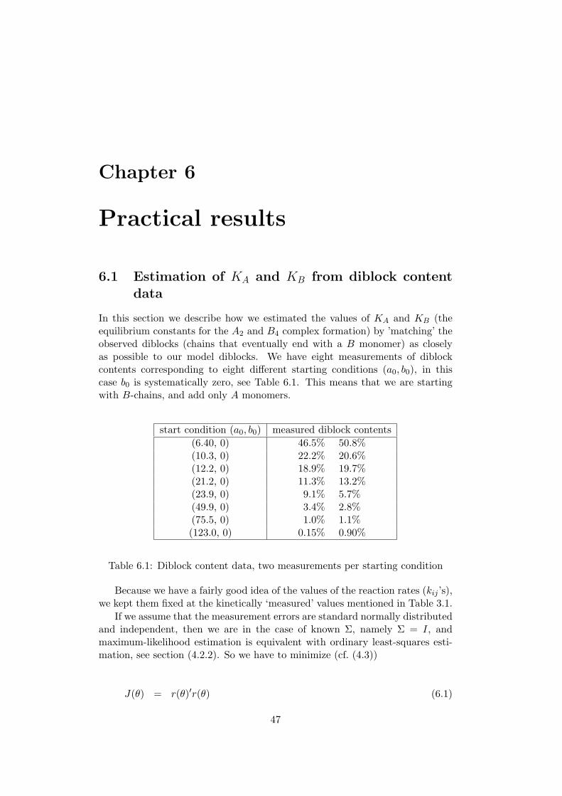
In this section we describe how we estimated the values of KA and KB (theequilibrium constants for the A2 and B4 complex formation) by ’matching’ theobserved diblocks (chains that eventually end with a B monomer) as closelyas possible to our model diblocks. We have eight measurements of diblockcontents corresponding to eight different starting conditions (a0, b0), in thiscase b0 is systematically zero, see Table 6.1. This means that we are startingwith B-chains, and add only A monomers.
start condition (a0, b0) measured diblock contents
(6.40, 0) 46.5% 50.8%(10.3, 0) 22.2% 20.6%(12.2, 0) 18.9% 19.7%(21.2, 0) 11.3% 13.2%(23.9, 0) 9.1% 5.7%(49.9, 0) 3.4% 2.8%(75.5, 0) 1.0% 1.1%(123.0, 0) 0.15% 0.90%
Table 6.1: Diblock content data, two measurements per starting condition
Because we have a fairly good idea of the values of the reaction rates (kij ’s),we kept them fixed at the kinetically ‘measured’ values mentioned in Table 3.1.
If we assume that the measurement errors are standard normally distributedand independent, then we are in the case of known Σ, namely Σ = I, andmaximum-likelihood estimation is equivalent with ordinary least-squares esti-mation, see section (4.2.2). So we have to minimize (cf. (4.3))
J(θ) = r(θ)′r(θ) (6.1)
47

48 CHAPTER 6. PRACTICAL RESULTS
=8∑
k=1
((observed diblock)k − (model diblock(θ))k)2 ,
where r(θ) is the vector of residuals and θ = (KA,KB).
However, this approach is based on the absolute error. So the large diblocks,which will occur when a0 is small, will dominate since the minimization proce-dure will try to keep the distance between large diblocks small. To overcomethis problem we could scale each residual. Because with each starting conditiontwo measurements were performed, we have a rough idea of the variation of eachmeasured diblock. Hence, we can estimate the diblock variance based on thesetwo points. The squared residuals are scaled by the corresponding estimateddiblock variance. Thus (6.1) becomes
J(θ) = r(θ)′Σ−1db r(θ) (6.2)
(6.3)
where Σdb is a diagonal matrix containing the estimated variances.
Since KA and KB could vary from zero to infinity, we scaled them for numericalconvenience, introducing the [0, 1] variables
KA =KA
1 +KA
KB =KB
1 +KB.
If we look at the plot of J(θ) in Fig.6.1, we see that J decreases in KB. Thismeans that our estimate of KB is
KB = ∞ .
This implies that the model in which there are no B4 aggregates, fits the ob-served data best.
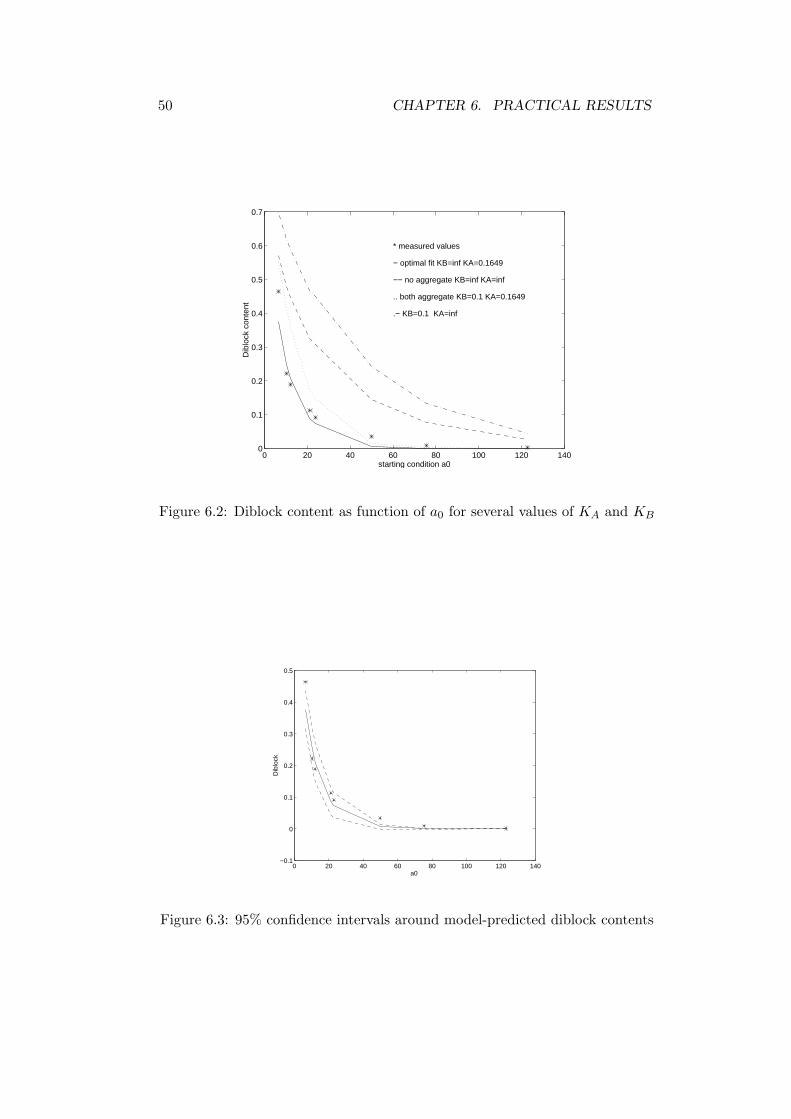
Thus by substituting KB = ∞ in our model we can subsequently minimizewith respect to KA. With the Simplex Search algorithm we found the estimateKA = 0.1649 with the 95% confidence interval (0.1171 ; 0.2127) using (4.2). InFig. (6.2) we plotted measured values with the predicted values of the diblockcontent as function of a0 for the estimated values of KA and KB, together withsome other values for KA and KB, to illustrate the quality of the fit. In additionthe 95% confidence intervals in the prediction domain are plotted, see Fig. 6.3indicating a very good explanation of the measured dependencies of diblock ona0. To illustrate what a value of 0.1649 for KA means for the ratio betweeneffective and active chains, see Fig.6.1. The time t runs along the curve, sinceat t = 0 there are no A-chains and gradually A chains are formed.
A model with B2 aggregates instead of B4 aggregates was also evaluated.The result was that the data was, again, best explained by a equilibrium con-stant (for B2 aggregates) with a value of infinity.

6.2. ESTIMATION OF REACTION RATES WITH NMR DATA 49
00.1
0.20.3
0.4
0.5
0.6
0.7
0.8
0.9
112
14
16
18
20
22
24
scaled KAscaled KB
Figure 6.1: plot of J(θ)
6.2 Estimation of reaction rates with NMR data
The next step is to estimate the four reaction rates. In practice one is onlyinterested in the ratio of the reaction rates. For, multiplying the four rateswith a fixed number has only effect on the absolute time scale of the reactions.Thus we can normalize the reaction rates with one of them. We then havethree remaining parameters, r1, r2 and r3, to be estimated. Their kineticallymeasured values are shown in Table 6.2, cf. Table 3.1.
ratio (measured) value
r1 =kaakba
45.83
r2 =kabkba
2120
r3 =kbbkba
10
Table 6.2: reaction ratios
The measured diblock contents were obtained through a homopolymeriza-tion, i.e. only A monomers were added to one mol B-chains. Thus only pa-rameter r1 plays a role in this particular case. This is why we tried to estimateKA (KB is pinned down at ∞) and r1 using diblock data only. If the − loglikelihood function is plotted (cf. fig 6.5), a banana-shaped (non-convex) valleyis observed where no minimum could be found. Therefore, the use of diblockdata only, is insufficient to estimate these parameters.Hence we need additional information to be able to say anything about thereaction rates.
Fortunately there are measurements of triad fractions available. Three tri-
50 CHAPTER 6. PRACTICAL RESULTS
0 20 40 60 80 100 120 1400
0.1
0.2
0.3
0.4
0.5
0.6
0.7
Dib
lock
con
tent
starting condition a0
* measured values
− optimal fit KB=inf KA=0.1649
−− no aggregate KB=inf KA=inf
.. both aggregate KB=0.1 KA=0.1649
.− KB=0.1 KA=inf
Figure 6.2: Diblock content as function of a0 for several values of KA and KB
0 20 40 60 80 100 120 140−0.1
0
0.1
0.2
0.3
0.4
0.5
a0
Dib
lock
Figure 6.3: 95% confidence intervals around model-predicted diblock contents

6.2. ESTIMATION OF REACTION RATES WITH NMR DATA 51
0 0.1 0.2 0.3 0.4 0.5 0.6 0.7 0.8 0.9 10
0.1
0.2
0.3
0.4
0.5
0.6
0.7
0.8
0.9
1
amount of active A−chains
frac
tion
ef
fect
ive
: act
ive
A−
chai
ns
Figure 6.4: fraction of the effective A chains- - - KA = 10 — KA = 0.1649 · · ·KA = 0.001
ads were measured, namely AAA, BAA and BAB, cf. Table 6.3. In order touse these triad data for an analysis we have to use our model with care. First,the triads are measured for the complete chains, while our model triad predic-tions are only based on their occurrence in the final block, i.e. propagationin phase 3. But this is easily dealt with, since phase 1 and 2 consist only ofa pure A block and a pure B block, with known length. Secondly, the NMRmachine is not able to distinguish the position of a polymer chain. Thereforethe measured BAA triad consists not only of BAA but of AAB as well, andthey must be combined in the model calculations. Finally the measured triadsare only proportions, while our model deals with absolute amounts of triads,this requires the computation of normalized triads under the model.
Normalized triad fractions
starting condition (a0, b0) AAA BAA BAB
(106, 9.81) 0.8786 0.1040 0.0173(106, 39.2) 0.8284 0.1001 0.0710(106, 108) 0.8278 0.1055 0.0666
Table 6.3: NMR data

52 CHAPTER 6. PRACTICAL RESULTS
0.10.2
0.30.4
0.50.6
0
0.2
0.4
0.6
0.8
110
15
20
25
30
35
scaled ratio1scaled KS
function plot of −log(lik)
Figure 6.5: plot of J
6.2.1 Identifiability check
The NMR spectrum clearly shows three separate peaks, so that we can assumethat the errors of the areas under the three peaks are independent and (2.1)becomes a diagonal matrix. Before we tried to estimate the three ratios r1, r2and r3, we investigated their identifiability by simulation and singular valuedecomposition. For the simulation we had to choose three r-values. We tookthe measured values and then simulated 20 repetitions of ( AAA, BAA andBAB) triad distributions with our model. When we successively fixed one r atthe measured value and calculated the two dimensional ’sub’ likelihood for thetwo others we got the global results as summarized in table 6.4.
fixed ratio shape ‘sub’ likelihood
r1 convex, with minimum values of r2, r3 close to their chosen valuesr2 convex, with minimum values of r1, r3 close to their chosen valuesr3 not convex, no minimum could be found
Table 6.4:
These results indicates that a problem would arise if we would estimate thethree r’s simultaneously. This conjecture was confirmed by singular value de-composition analyses. We have the three model predicted triads
ypred(θ) =
AAABAABAB
,

6.2. ESTIMATION OF REACTION RATES WITH NMR DATA 53
where θ = (r1, r2, r3).The sensitivity matrix S(θ), with respect to changes in ln(θ), is
S(θ) =∂ypred(θ)
∂ ln θ.
Using the ideas of section (4.3) we performed a singular value decompositionon S(θ), and found
S = UDV
U =
−0.5372 −0.6150 0.57720.8012 −0.1584 0.5770
−0.2634 0.7725 0.5778
, (6.4)
D =
0.0469 0 00 0.0240 00 0 0.0000
, (6.5)
V =
0.6677 −0.6403 −0.3796−0.2683 0.2686 −0.92510.6944 0.7169 0.0075
. (6.6)
From this we see that the third singular value is zero (at least numerically)and therefore at least one combination of the r’s is not identifiable. The cor-responding (third) row of V shows which r’s are involved, it indicates that thecombination of parameter perturbations
0.6944 ln(r1) + 0.7169 ln(r2) + 0.0075 ln(r3)
is ill conditioned in the sense that any change in the parameter space in thedirection of that combination will not induce any change in the model predictedvalues. Consequently the product r1r2 is ill conditioned and can not be iden-tified from the given triad data, as the coefficient 0.0075 for r3 is negligiblerelative to the other coefficients.
So we had to fix either r1 or r2 on their measured value, we chose to fix r2.Because the equilibrium constants KA and KB have very little impact on thetriads in our model, we kept them fixed at the earlier estimated values. Usingboth diblock data and NMR data, for estimating our parameters r1 and r3 wenow have to minimize
J(θ) = rdb(θ)′Σ−1
db rdb(θ) + rnmr(θ)′Σ−1
nmrrnmr(θ) (6.7)
= J1 + J2 , (6.8)
(6.9)
where θ = (r1, r3). A plot of the likelihood function is shown in Fig. 6.6. Weobtained estimated values r1 and r3 as given in tabel 6.5 .
As in the case with the diblock data, we scaled squared residuals by the es-timated variances of the diblocks. However, with NMR data we have no precise

54 CHAPTER 6. PRACTICAL RESULTS
ratio
estimated value(95% confidence)
kinetically measuredvalue
r1 =kaakba
45.48 (± 7.77) 45.833
r3 =kbbkba
4.94 (± 8.20) 10
Table 6.5: estimated values
00.1
0.20.3
0.40.5
0.2
0.3
0.4
0.5
0.6
0.75.5
6
6.5
7
7.5
scaled ratio3 (kbb/kba)scaled ratio1 (kaa/kba)
Figure 6.6: plot of -log(likelihood)
idea of the absolute accuracy of the NMR measurements, since only one dataset per start condition is available. Usually one then scales the squared residu-als ‘psychological’, i.e. both squared residuals are made to be of the same orderof magnitude, J1 ≈ J2. If we plot the NMR data together with the predictedvalues, we get an indication of the quality of the fit, the dotted bars are the95% intervals around model-predicted triads, see Fig. 6.7 and 6.8 for the twodifferent sets of values of the starting conditions a0 and b0. We notice that the95% intervals around the predictions only covers the measured triad fractionBAB, indicating a lesser fit than in the diblock domain. A reason for this couldbe the extreme sensitivity of the triads on the starting conditions. In practicethe amounts of reagent are not determined before the reactions, they are deter-mined afterwards. Hence, it is likely that the obtained starting conditions aresubjected to inaccuracies

6.2. ESTIMATION OF REACTION RATES WITH NMR DATA 55
0.5 1 1.5 2 2.5 3 3.50
0.1
0.2
0.3
0.4
0.5
0.6
0.7
0.8
0.9
1Triad ratios
AAA BAA BAB
Figure 6.7: - - - model predicted, — measured, start conditions a0 = 106 b0 =9.8
0.5 1 1.5 2 2.5 3 3.50
0.1
0.2
0.3
0.4
0.5
0.6
0.7
0.8
0.9Triad ratios
BABBAAAAA
Figure 6.8: - - - model predicted, — measured, start conditions a0 = 106 b0 =39.2
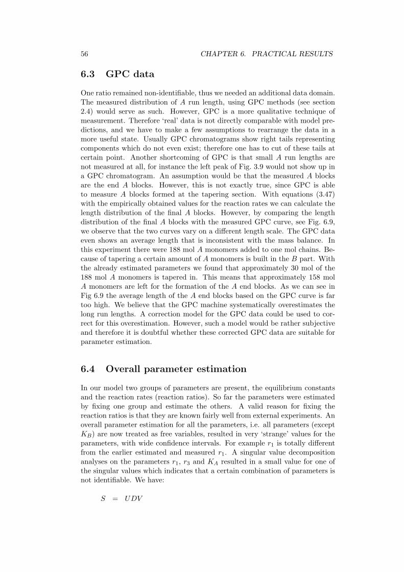
56 CHAPTER 6. PRACTICAL RESULTS
6.3 GPC data
One ratio remained non-identifiable, thus we needed an additional data domain.The measured distribution of A run length, using GPC methods (see section2.4) would serve as such. However, GPC is a more qualitative technique ofmeasurement. Therefore ‘real’ data is not directly comparable with model pre-dictions, and we have to make a few assumptions to rearrange the data in amore useful state. Usually GPC chromatograms show right tails representingcomponents which do not even exist; therefore one has to cut of these tails atcertain point. Another shortcoming of GPC is that small A run lengths arenot measured at all, for instance the left peak of Fig. 3.9 would not show up ina GPC chromatogram. An assumption would be that the measured A blocksare the end A blocks. However, this is not exactly true, since GPC is ableto measure A blocks formed at the tapering section. With equations (3.47)with the empirically obtained values for the reaction rates we can calculate thelength distribution of the final A blocks. However, by comparing the lengthdistribution of the final A blocks with the measured GPC curve, see Fig. 6.9,we observe that the two curves vary on a different length scale. The GPC dataeven shows an average length that is inconsistent with the mass balance. Inthis experiment there were 188 mol A monomers added to one mol chains. Be-cause of tapering a certain amount of A monomers is built in the B part. Withthe already estimated parameters we found that approximately 30 mol of the188 mol A monomers is tapered in. This means that approximately 158 molA monomers are left for the formation of the A end blocks. As we can see inFig 6.9 the average length of the A end blocks based on the GPC curve is fartoo high. We believe that the GPC machine systematically overestimates thelong run lengths. A correction model for the GPC data could be used to cor-rect for this overestimation. However, such a model would be rather subjectiveand therefore it is doubtful whether these corrected GPC data are suitable forparameter estimation.
6.4 Overall parameter estimation
In our model two groups of parameters are present, the equilibrium constantsand the reaction rates (reaction ratios). So far the parameters were estimatedby fixing one group and estimate the others. A valid reason for fixing thereaction ratios is that they are known fairly well from external experiments. Anoverall parameter estimation for all the parameters, i.e. all parameters (exceptKB) are now treated as free variables, resulted in very ‘strange’ values for theparameters, with wide confidence intervals. For example r1 is totally differentfrom the earlier estimated and measured r1. A singular value decompositionanalyses on the parameters r1, r3 and KA resulted in a small value for one ofthe singular values which indicates that a certain combination of parameters isnot identifiable. We have:
S = UDV

6.5. AMOUNT OF TAPERING 57
0 100 200 300 400 500 600 700 8000
0.005
0.01
0.015
0.02
0.025
Length
−− GPC curve − predicted final A blocks
Figure 6.9: comparison of GPC curve and predicted length of final A blocks
D =
0.5099 0 00 0.0113 00 0 0.0076
(6.10)
V =
0.9111 −0.0003 0.4123−0.2434 0.8067 0.53860.3327 0.5910 −0.7348
. (6.11)
U is an 11 by 11 matrix and not relevant to give here. The third row of V(it corresponds with the small singular value) indicates that the parametercombination
0.3327 log(r1) + 0.5910 log(r3)− 0.7348 log(KS)
is badly conditioned. One reason could be that the two data domains (diblockcontent and triad fractions) are ‘separate’ domains. That is, the equilibriumconstants have almost no effect on the triad structures, while on the other handthe diblocks are formed by homopolymerization. Thus only one reaction ratio(r1 = kaa
kba) has effect on the diblocks. This insensitivity of certain parameters
on the prediction causes (near) invariance of the likelihood in some sub-spaces.Therefore a proper estimation is very difficult or even impossible. We note thatthe available data were never collected for the aim of parameter estimation. Thevariation in the data is merely caused by the difference in starting conditions.
6.5 Amount of tapering
As we mentioned in the introduction, tapering strongly influences product prop-erties. With the derived model for copolymerization, we are now in a position

58 CHAPTER 6. PRACTICAL RESULTS
to predict the ‘amount of tapering’, i.e. the amount of A monomers that hasreacted with the living chain before exhaustion of B monomers (cf. Fig. 3.3).Also interesting is the single tapered A monomers, which correspond with thetriad structure BAB (cf. eq. (3.46)). Although our model describes only phase3 (see section 1.2), a complete chain consists of three phases. The first phasehas a0 A monomers, and therefore the total amount of A monomers for a com-plete triblock is 2a0. We compared the tapered A monomers with this quantity,The results are summarized in tabel 6.6 and Fig. 6.10.
startingcondition(a0, b0)
amountof tapering
(mol)percentage of
2a0
percentage singletapered A monomers
(106, 9.81) 18.33 8.65 2.31(106, 39.2) 32.23 15.2 8.23(106, 108) 46.13 21.8 14.8(106, 304) 57.16 26.9 21.9(106, 520) 63.78 30.1 25.2(106, 981) 69.23 32.6 28.7
Table 6.6: Amount of tapering
0 100 200 300 400 500 600 700 800 900 10000
5
10
15
20
25
30
35
Amount of b0
perc
enta
ge o
f tap
erin
g
Figure 6.10: — total tapered A - - - single tapered (= isolated) A

Chapter 7
Summary and Conclusions
In this report a model is derived, in order to estimate parameters of a nonsta-tionary Markov model for copolymer propagation with two types of monomers,A and B. This model can be used to predict the chain characteristics. Severalcharacteristics of the polymer chains, length, weight, triad structures and block(run) length distribution are modelled with a set of differential equations. Wehave numerically checked model consistency, with (probability) mass-balancechecks. For example the probability of triad structure BAB must be equal tothe probability of run length one of A. Also the expected length of the chainsmust equal to the amount of added monomers.
Algebraic equations are added to the model, to describe the phenomenonthat active chains can aggregate to non-reactive clusters.
We note that this model can be extended for more than two types ofmonomers. Extra differential equations for the other types are then addedto the model, these equations are derived at the same way.
Differential equations are derived that describe the sample-averaged monomerstatistics, i.e. the ‘average’ molecule will obey these equations. To obtain in-formation about the effect of the random fluctuations, one e.g. has to simulateeach individual reaction of a large amount of chains. However these fluctua-tions are neglictable for the relative changes in the concentration of monomersbecause of the large numbers of molecules.
Runge-Kutta methods were initially used to solve the model equations; how-ever numerical problems related to stiffness suggested the use of implicit meth-ods. However the explicit; relative simple Bulirsch-Stoer extrapolation methodyielded quit good results in conjunction with the parameter estimation routinesthat require the ODE solutions.
The comparison of modelled with measured diblock fractions indicates thatthe data is best explained by aggregated A-chains and totally free B-chains. Wefound that the aggregate forming had very little effect on the triad statistics.Using NMR and diblock data together it was possible to get a value for twoof the three reaction ratio’s, r1 = kaa
kbaand r3 = kbb
kba. The values correspond
with measured values, which were obtained in a totally different way. To get abetter insight into ratio r2 = kab
kbawe are in need of an additional data domain.
However it appeared that the A run length GPC data, was too unreliable to be
59

60 CHAPTER 7. SUMMARY AND CONCLUSIONS
used for parameter estimation.In the current experiments, data has been collected once for every (batch)
operating condition. One has to scale ‘psychologically’ to balance the infor-mation in diblock content and NMR-data more or less equally. However, withrepetitive data, one could obtain a better understanding of the variances, allow-ing the residuals to be weighted according to their corresponding (estimated)variances.
A recommendation would be the use of a totally different data domain,such as data related to the kinetics of the chemical reactions. One measuresthe concentration of the monomers, or other chain characteristics, at some(fixed) times ti. These quantities could then be compared with model-predictedquantities at time ti. It is obvious that these data reveal more informationthan only the characteristics of a polymer chain at the end of the reaction. Forexample, an expected chain length at the end of the reaction tells us nothingabout the parameters, since due to mass balance this expected length mustequal to the amount of monomers added, while the progress of the expectedlength during the reaction is very informative. However there are practicallimitations to obtain chain characteristics during the reactions and therefore nodata concerning the kinetics were available yet.

Bibliography
[1] W.H. Greene, Econometric Analysis, Macmillan 1990.
[2] G.C. Goodwin, R.L. Payne, Dynamical System Identification AcademicPress 1977.
[3] J.C. Randall, Polymer Sequence Determination, Academic Press 1977.
[4] K.H. Altgelt, L. Segal, Gel Permeation Chromatography, Marcel Dekker,Inc. 1971.
[5] L. Ameraal, C++, Academic service 1992.
[6] A.J. Staverman, macromoleculen, Leidse uitgeverij 1981.
[7] M.W. van der Burg, J.C. Chadwick, O. Sudmeijer, H.J.A.F. Tulleken,Makromol. Chem., Theory Simul. 2, 385 (1993)
[8] P.E. Gill, M.H. Wright, Practical Optimization, Academic Press 1981.
[9] W.H. Press, S.A. Teukolsky, W.T. Vetterling, Numerical Recipes in C,Cambridge University Press 1992.
[10] R. Bulirsch, J. Stoer, Introduction to Numerical Analysis, Springer-Verlag1980.
[11] The Mathworks, Inc, South Nattick, Massachusetts, MATLAB user’sGuide, August 1992.
61

62 BIBLIOGRAPHY

Appendix A
Computer program
The solver for the differential equations is programmed in C, and can be foundin [9]. Two adjustments are made. First the stopping criterion is changed: thesolver now stops when the amounts of monomers drop below a certain level,i.e. the reaction is finished, instead of stopped at a fixed time. Secondly aMATLAB gateway has been written to create a so called ‘MEX file’, see [11].The great advantage of this is that once the gateway has been created, theC codes can be activated within MATLAB, and therefore can be combinedwith standard MATLAB commands. The codes given below, consist of thegateway function and a function odeint that arranges the Bulirsch-Stoer stepsand checks whether the reaction is finished.
#include <math.h>
#include "nrutil.h"
#include "mex.h"
#include "nr.h"
#define NRANSI
#define MAXSTP 100000
#define TINY 1.0e-30
/******************************************/
/* */
/* COMPUTATIONAL ROUTINE */
/* odeABA.c */
/* */
/* This routine solves the ode y’=f(y) */
/* using Bulirsch-Stoer method, output */
/* xp = time were the reaction has */
/* finished. */
/* yp = state vector at time xp */
/* required input are: */
/* ystart := initial conditions */
/* para := vector of parameters */
/* nvar := number of variables */
63

64 APPENDIX A. COMPUTER PROGRAM
/* x1 := begin time of integration */
/* eps := required accuracy */
/* h1 := initial stepsize */
/* hmin := minimum stepsize */
/* */
/******************************************/
void odeint(double ystart[], double para[],int nvar, double x1,
double eps, double h1,
double hmin,
double *xp, double yp[])
/* This function uses derivs.c and bsstep.c, in derivs.c the diff. equations */
/* are programmed. In bsstep.c one Bulirsch-Stoer step is carried out. */
{
int nstp,i;
double xsav,x,hnext,hdid,h;
double *yscal,*y,*dydx;
yscal=dvector(1,nvar);
y=dvector(1,nvar);
dydx=dvector(1,nvar);
x=x1;
h=h1;
for (i=1;i<=nvar;i++) y[i]=ystart[i-1];
for (nstp=1;nstp<=MAXSTP;nstp++){
derivs(x,y,dydx,para);
for (i=1;i<=nvar;i++) yscal[i]=fabs(y[i])+fabs(dydx[i]*h)+TINY;
bsstep(y,dydx,nvar,&x,h,eps,yscal,&hdid,&hnext,para);
if (y[2] <= ystart[1])*1e-4){ /* Is the reaction completed? */
*xp=x;
for (i=1;i<=nvar;i++){ yp[i-1]=y[i];}
free_dvector(dydx,1,nvar);
free_dvector(y,1,nvar);
free_dvector(yscal,1,nvar);
return; }
h=hnext; }
nrerror("Too many steps");
}
#undef MAXSTP
#undef TINY
#undef NRANSI
/************************************/

65
/* */
/* GATEWAY ROUTINE */
/* odeABA.c */
/* */
/************************************/
void mexFunction(int nlhs,Matrix *plhs[],int nrhs,Matrix *prhs[])
{
double *ystart;
double *xp, *yp;
int nvar;
double *para;
double x1,eps;
double h1,hmin;
unsigned int k,l;
int m;
/* check for proper number of arguments */
if (nrhs != 8)
{ mexErrMsgTxt(" 8 input arguments required.");}
else if (nlhs !=2)
{ mexErrMsgTxt(" 2 output arguments required.");}
/* ystart must be of size 19x1 */
k = mxGetM(prhs[0]);
l = mxGetN(prhs[0]);
if (!mxIsNumeric(prhs[0]) || mxIsComplex(prhs[0]) ||
!mxIsDouble(prhs[0]) ||
!(k==19 && l==1))
{ mexErrMsgTxt(" Ystart must be a vector of length 19");}
/* nvar must be of size 1x1 */
k = mxGetM(prhs[1]);
l = mxGetN(prhs[1]);
if (!mxIsNumeric(prhs[1]) || !mxIsDouble(prhs[1]) ||
!(k==1 && l==1))
{ mexErrMsgTxt(" nvar must be scalair ");}
/* para must be of size 6x1 */
k = mxGetM(prhs[2]);
l = mxGetN(prhs[2]);
if (!mxIsNumeric(prhs[2]) || !mxIsDouble(prhs[2]) ||

66 APPENDIX A. COMPUTER PROGRAM
!mxIsFull(prhs[2]) || !mxIsDouble(prhs[2]) ||
!(k==6 && l==1))
{ mexErrMsgTxt(" para must be a vector of length 6 ");}
/* x1 must be of size 1x1 */
k = mxGetM(prhs[3]);
l = mxGetN(prhs[3]);
if (!mxIsNumeric(prhs[3]) || !mxIsDouble(prhs[3]) ||
!(k==1 && l==1))
{ mexErrMsgTxt(" x1 must be scalair ");}
/* eps must be of size 1x1 */
k = mxGetM(prhs[4]);
l = mxGetN(prhs[4]);
if (!mxIsNumeric(prhs[4]) || !mxIsDouble(prhs[4]) ||
!(k==1 && l==1))
{ mexErrMsgTxt(" eps must be scalair ");}
/* h1 must be of size 1x1 */
k = mxGetM(prhs[5]);
l = mxGetN(prhs[5]);
if (!mxIsNumeric(prhs[5]) || !mxIsDouble(prhs[5]) ||
!(k==1 && l==1))
{ mexErrMsgTxt(" h1 must be scalair ");}
/* hmin must be of size 1x1 */
k = mxGetM(prhs[6]);
l = mxGetN(prhs[6]);
if (!mxIsNumeric(prhs[6]) || !mxIsDouble(prhs[6]) ||
!(k==1 && l==1))
{ mexErrMsgTxt(" hmin must be scalair ");}
/* create matrix for the return argument. */
/* nvar is the number of state variables */
/* and should be given a specific value */
/* when using this routine */
plhs[0] = mxCreateFull(1,1, REAL);
plhs[1] = mxCreateFull(nvar,1, REAL);
/* dereference arguments and call the computational routine */

67
xp = mxGetPr(plhs[0]);
yp = mxGetPr(plhs[1]);
ystart = mxGetPr(prhs[0]);
nvar = *mxGetPr(prhs[1]);
para = mxGetPr(prhs[2]);
x1 = *mxGetPr(prhs[3]);
eps = *mxGetPr(prhs[4]);
h1 = *mxGetPr(prhs[5]);
hmin = *mxGetPr(prhs[6]);
odeint( ystart,para, nvar,x1,eps,h1,hmin, xp, yp);
}

68 APPENDIX A. COMPUTER PROGRAM

Appendix B
Matrix differentiation rules
In this appendix we shall give some useful matrix differentiation rules. Theseresults are used in maximum likelihood estimation (see chapter 4).
Result 1 for a symmetric matrix A ∂∂xx
′Ax = 2Ax.
proof:Let x = (x1, . . . , xn) and let the i,m-th element of A defined by aim then it issufficient to show that
∂
∂xi(x′Ax) = (2Ax)i = 2
∑m
aimxm .
We find
∂
∂xi(x′Ax) =
∂
∂xi(∑k
∑m
xkakmxm)
=∑k=i
∑m=i
∂
∂xixkakmxm +
∑k =i
∑m=i
∂
∂xixkakmxm +
∂
∂xixiaiixi
= 2∑m=i
∂
∂xi(xiaimxm) +
∂
∂xiaiix
2i
= 2∑m=i
aimxm + 2aiixi
= 2∑m
aimxm = (2Ax)i 2
Derivatives involving determinants and traces can also be calculated.
Result 2 For any invertible matrix A,
∂ ln |A|∂A
= (A−1)′
Proof:From cofactorization of a matrix A we know that
69

70 APPENDIX B. MATRIX DIFFERENTIATION RULES
|A| =k∑
j=1
aij(−1)i+j |Aij | ,
where Aij is the matrix obtained by deleting the i-th column and j-th row andk is the dimension of A. When the correct sign (−1)i+j is added, it becomes acofactor.Hence
∂ |A|∂aij
= (−1)i+j |Cji|
where |Cij | is the ij-th cofactor in A. Notice the reversal in subscripts.
The inverse of A can be computed using
a−1ij =
(−1)i+j |Cij ||A|
,
which implies:∂ ln |A|∂aij
=(−1)i+j |Cji|
|A|.
Collecting terms we get
∂ ln |A|∂A
= (A−1)′ 2
Result 3 For any matrix W and invertible matrix A,
∂
∂Atrace(WA−1) = −(A−1WA−1)′
Proof:Since
AA−1 = I ,
we have∂A
∂aijA−1 +A
∂A−1
∂aij= 0 .
Hence∂A−1
∂aij= −A−1 ∂A
∂aijA−1 = −A−1eie
′jA
−1 ,
and therefore
∂
∂aijtrace(WA−1) = trace
(W
∂A−1
∂aij
)= −trace
(WA−1eie
′jA
−1)
= −e′jA−1WA−1ei = −ei
(A−1WA−1
)′ej .
By collecting terms we get
∂
∂Atrace(WA−1) = −(A−1WA−1)′ 2